notes on the euler equations - stony brook...

Notes on the Euler Equations

These notes describe how to do a piecewise linear or piecewise parabolic method for the Euler equations.

1 Euler equation properties

The Euler equations in one dimension appear as:

∂ρ

∂t+

∂(ρu)

∂x= 0 (1)

∂(ρu)

∂t+

∂(ρuu + p)

∂x= 0 (2)

∂(ρE)

∂t+

∂(ρuE + up)

∂x= 0 (3)

These represent conservation of mass, momentum, and energy. Here ρ is the density, u is the one-dimensional velocity, p is the pressure, and E is the total energy / mass, and can be expressed in terms ofthe specific internal energy and kinetic energies as:

E = e +1

2u2 (4)

The equations are closed with the addition of an equation of state:

p = ρe(γ− 1) (5)

where γ is the ratio of specific heats for the gas/fluid (for an ideal, monatomic gas, γ = 5/3).In this form, the equations are said to be in conservative form. They can be written as:

Ut + [F(U)]x = 0 (6)

with

U =

ρρuρE

F(U) =

ρuρuu + p

ρuE + up

(7)

An alternate way to express these equations is using the primitive variables: ρ, u, p.

Exercise 1: Show that the Euler equations in primitive form can be written as

qt + A(q)qx = 0 (8)

where

q =

ρup

A(q) =

u ρ 00 u 1/ρ0 γp u

(9)

The eigenvalues of A can be found via |A− λI| = 0, where | . . . | indicates the determinant and λ are theeigenvalues.

Exercise 2: Show that the eigenvalues of A are λ(−) = u− c, λ(◦) = u, λ(+) = u + c where the speedof sound is c =

√γp/ρ.

M. Zingale—Notes on the Euler equations1

(April 16, 2013)

We’ll use the symbols {−, ◦,+} to denote the eigenvalues and their corresponding eigenvectors though-out these notes. These eigenvalues are the speeds at which information propagates for the fluid equations.Since the eigenvalues are real, this system (the Euler equations) is said to be hyperbolic. Additionally, sinceA = A(q), the system is said to be quasi-linear. The right and left eigenvectors can be found via:

A r(ν) = λ(ν)r(ν) ; l(ν) A = λ(ν)l(ν) (10)

where ν = {−, ◦,+} corresponding to the three waves, and there is one right and one left eigenvector foreach of the eigenvalues.

Exercise 3: Show that the right eigenvectors are:

r(−) =

1−c/ρ

c2

r(◦) =

100

r(+) =

1c/ρc2

(11)

and the left eigenvectors are:

l(−) =(

0 − ρ2c

12c2

)l(◦) =

(1 0 − 1

c2

)l(+) =

(0

ρ2c

12c2

)(12)

Note that in general, there can be an arbitrary constant in front of each eigenvector. Here they arenormalized such that l(i) · r(j) = δij.

A final form of the equations is called the characteristic form. Here, we wish to diagonalize the matrix A.We take the matrix R to be the matrix of right eigenvectors, R = (r(−)|r(◦)|r(+)), and L is the correspondingmatrix of left eigenvectors. Note that L R = I = R L, and L = R−1.

Exercise 4: Show that Λ = LAR is a diagonal matrix with the diagonal elements simply the 3 eigen-values we found above.

Defining dw = Ldq, we can write our system as:

wt + Λwx = 0 (13)

Here, the w are the characteristic variables. Note that we cannot in general integrate dw = Ldq to writedown the characteristic quantities. Since Λ is diagonal, this system is a set of decoupled advection-likeequations. If the system were linear, then the solution to each would simply be to advect the quantity w(ν)

at the wave speed λ(ν).The way to think about this system is that there are 3 wave speeds (one for each eigenvalue) and each

wave carries with it a change in the characteristic variable. Since dq = L−1dw = Rdw, the jump in theprimitive variable across each wave is proportion to the right-eigenvector associated with that wave. So,for example, since r(◦) is only non-zero for the density element, this then means that only density jumpsacross the λ(◦) = u wave—pressure and velocity are constant across this wave (see for example, Toro [12],Ch. 2, 3 or LeVeque [7] for a thorough discussion). Figure 1 shows the three waves emanating from aninitial discontinuity.

2 Reconstruction of interface states

We will solve the Euler equations using a high-order Godunov method—a finite volume method wherebythe fluxes through the interfaces are computed by solving the Riemann problem for our system. Thefinite-volume update for our system appears as:

Un+1i = Un

i +∆t

∆x

(Fn+1/2

i−1/2 − Fn+1/2i+1/2

)(14)


(April 16, 2013)

0.1

0.2

0.3

0.4

0.5

0.6

0.7

0.8

0.9

1

0 0.1 0.2 0.3 0.4 0.5 0.6 0.7 0.8 0.9 1

densit

y

x

0 0.1 0.2 0.3 0.4 0.5 0.6 0.7 0.8 0.9

1

0 0.1 0.2 0.3 0.4 0.5 0.6 0.7 0.8 0.9 1

velo

cit

y

x

0.1

0.2

0.3

0.4

0.5

0.6

0.7

0.8

0.9

1

0 0.1 0.2 0.3 0.4 0.5 0.6 0.7 0.8 0.9 1

pre

ssure

x

Figure 1: Evolution following from an initial discontinuity at x = 0.5. These particular conditions arecalled the Sod problem, and in general, a setup with two states separated by a discontinuity is calleda shock-tube problem. Here we see the three waves propagating away from the initial discontinuity.The left (u− c) wave is a rarefaction, the middle (u) is the contact discontinuity, and the right (u + c)is a shock. Note that all 3 primitive variables jump across the left and right waves, but only thedensity jumps across the middle wave. This reflects the right eigenvectors.


(April 16, 2013)

i i+1i+1/2

Un+1/2

i+1/2,LUi U

n+1/2

i+1/2,RUi+1

F(Un+1/2

i+1/2)

Figure 2: The left and right states at interface i + 1/2. The arrow indicates the flux through theinterface, as computed by the Riemann solver using these states as input.

This says that each of the conserved quantities in U change only due to the flux of that quantity throughthe boundary of the cell.

Instead of approximating the flux itself on the interface, we find an approximation to the state on the

interface, Un+1/2i−1/2 and Un+1/2

i+1/2 and use this with the flux function to define the flux through the interface:

Fn+1/2i−1/2 = F(Un+1/2

i−1/2 ) (15)

Fn+1/2i+1/2 = F(Un+1/2

i+1/2 ) (16)

To find this interface state, we predict left and right states at each interface (centered in time), which arethe input to the Riemann solver. The Riemann solver will then look at the characteristic wave structureand determine the fluid state on the interface, which is then used to compute the flux. This is illustratedin Figure 2. The fluxes allow us to update the state in time as:

Un+1i = Un

i +∆t

∆x

(Fn+1/2

i−1/2 − Fn+1/2i+1/2

)(17)

Finally, although we use the conserved variables for the final update, in constructing the interfacestates it is often easier to work with the primitive variables. These have a simpler characteristic structure.The interface states in terms of the primitive variables can be converted into the interface states of theconserved variables through a simple algebraic transformation.

Constructing these interface states requires reconstructing the cell-average data with a piecewise con-stant, linear, or parabolic polynomial and doing characteristic tracing to see how much of each charac-teristic quantity comes to the interface over ∆t/2. Since we are comfortable working with the primitivevariables, the reconstruction is done on those, and they are then projected into the characteristic variables(using the left- and right-eigenvectors) to determine how much of each characteristic quantity is carriedby each of the 3 waves. We look at several methods below.

2.1 Piecewise constant

The simplest possible reconstruction of the data is piecewise constant. This is what was done in theoriginal Godunov method. For the interface marked by i + 1/2, the left and right states on the interfaceare simply:

Ui+1/2,L = Ui (18)

Ui+1/2,R = Ui+1 (19)

This does not take into account in any way how the state U may be changing through the cell. As aresult, it is first-order accurate in space, and since no attempt was made to center it in time, it is first-orderaccurate in time.


(April 16, 2013)

ii−1 i+1i−2 i+2

Figure 3: Piecewise linear reconstruction of the cell averages. The dotted line shows the unlimitedcenter-difference slopes and the solid line shows the limited slopes.

2.2 Piecewise linear

For higher-order reconstruction, we first convert from the conserved variables, U, to the primitive vari-ables, q. These have a simpler characteristic structure, making them easier to work with. Here we con-sider piecewise linear reconstruction—the cell average data is approximated by a line with non-zero slopewithin each cell. Figure 3 shows the piecewise linear reconstruction of some data.

Consider constructing the left state at the interface i + 1/2 (see Figure 2). Just like for the advectionequation, we do a Taylor expansion through ∆x/2 to bring us to the interface, and ∆t/2 to bring us to themidpoint in time. Starting with qi, the cell-centered primitive variable, expanding to the right interface(to create the left state there) gives:

qn+1/2i+1/2,L = qn

i +∆x

2

∂q

∂x

∣∣∣∣i

+∆t

2

∂q

∂t

∣∣∣∣i︸︷︷︸

=−A∂q/∂x

+ . . . (20)

= qni +

∆x

2

∂q

∂x

∣∣∣∣i

− ∆t

2

(A

∂q

∂x

)

i

(21)

= qni +

1

2

[1− ∆t

∆xAi

]∆qi (22)

where ∆qi is the reconstructed slope of the primitive variable in that cell (similar to how we compute itfor the advection equation). We note that the terms truncated in the first line are O(∆x2) and O(∆t2), soour method will be second-order accurate in space and time.

As with the advection equation, we limit the slope such that no new minima or maxima are intro-duced. Any of the slope limiters used for linear advection apply here as well. We represent the limitedslope as ∆qi.

We can decompose A∆q in terms of the left and right eigenvectors and sum over all the waves thatmove toward the interface. First, we recognize that A = RΛL and recognizing that the ‘1’ in Eq. 22 is theidentity, I = LR, we rewrite this expression as:

qn+1/2i+1/2,L = qn

i +1

2

[RL− ∆t

∆xRΛL

]

i

∆qi (23)

We see the common factor of L∆q. We now write this back in component form. Consider:

RΛL∆q =

r(−)1 r

(◦)1 r

(+)1

r(−)2 r

(◦)2 r

(+)2

r(−)3 r

(◦)3 r

(+)3

λ(−)

λ(◦)

λ(+)

l(−)1 l

(−)2 l

(−)3

l(◦)1 l

(◦)2 l

(◦)3

l(+)1 l

(+)2 l

(+)3

∆ρ

∆u

∆p

(24)


(April 16, 2013)

Starting with L∆q, which is a vector with each component the dot-product of a left eigenvalue with ∆q,we have

RΛL∆q =

r(−)1 r

(◦)1 r

(+)1

r(−)2 r

(◦)2 r

(+)2

r(−)3 r

(◦)3 r

(+)3

λ(−)

λ(◦)

λ(+)

l(−) · ∆q

l(◦) · ∆q

l(+) · ∆q

(25)

Next we see that multiplying this vector by Λ simply puts the eigenvalue with its respective eigenvectorin the resulting column vector:

RΛL∆q =

r(−)1 r

(◦)1 r

(+)1

r(−)2 r

(◦)2 r

(+)2

r(−)3 r

(◦)3 r

(+)3

λ(−) l(−) · ∆q

λ(◦) l(◦) · ∆q

λ(+) l(+) · ∆q

(26)

Finally, the last multiply results in a column vector:

RΛL∆q =

r(−)1 λ(−) l(−) · ∆q + r

(◦)1 λ(◦) l(◦) · ∆q + r

(+)1 λ(+) l(+) · ∆q

r(−)2 λ(−) l(−) · ∆q + r

(◦)2 λ(◦) l(◦) · ∆q + r

(+)2 λ(+) l(+) · ∆q

r(−)3 λ(−) l(−) · ∆q + r

(◦)3 λ(◦) l(◦) · ∆q + r

(+)3 λ(+) l(+) · ∆q

(27)

We can rewrite this compactly as:

∑ν

λ(ν)(l(ν) · ∆q)r(ν) (28)

where we use ν to indicate which wave we are summing over. A similar expansion is used for RL∆q. Theresulting vector for the left state is:

qn+1/2i+1/2,L = qn

i +1

2 ∑ν;λ(ν)≥0

[1− ∆t

∆xλ(ν)i

](l(ν)i · ∆qi)r

(ν)i (29)

Note that we make a slight change here, and only include a term in the sum if its wave is moving towardthe interface (λ(ν) ≥ 0).

Starting with the data in the i + 1 zone and expanding to the left, we can find the right state on thei + 1/2 interface:

qn+1/2i+1/2,R = qn

i+1 −1

2 ∑ν;λ(ν)≤0

[1 +

∆t

∆xλ(ν)i+1

](l(ν)i+1 · ∆qi+1)r

(ν)i+1 (30)

A good discussion of this is in Miller & Colella [8] (Eq. 85). This expression is saying that each wavecarries a jump in r(ν) and only those jumps moving toward the interface contribute to our interface state.This restriction of only summing up the waves moving toward the interface is sometimes called charac-teristic tracing. This decomposition in terms of the eigenvectors and eigenvalues is commonly called acharacteristic projection. In terms of an operator, P, it can be expressed as:

Pχ = ∑ν

(l(ν).χ)r(ν) (31)

Exercise 5: Show that Pq = q, using the eigenvectors corresponding to the primitive variable form ofthe Euler equations.

In the literature, sometimes a ‘>’ or ‘<’ subscript on P is used to indicate the characteristic tracing.We could stop here, but Colella & Glaz [4] (p. 278) argue that the act of decomposing A in terms of

the left and right eigenvectors is a linearization of the quasi-linear system, and we should minimize the


(April 16, 2013)

size of the quantities that are subjected to this characteristic projection. To accomplish this, they suggestsubtracting off a reference state. Saltzman (Eq. 8) further argues that since only jumps in the solution areused in constructing the interface state, and that the characteristic decomposition simply adds up all thesejumps, we can subtract off the reference state and project the result. In other words, we can write:

qn+1/2i+1/2,L − qref = qn

i − qref +1

2

[1− ∆t

∆xAi

]∆qi (32)

Then we subject the RHS to the characteristic projection—this tells us how much of the quantity qn+1/2i+1/2,L−

qref reaches the interface. Colella & Glaz (p. 278) and Colella (Eq. 2.11) suggest

qref = qi,L ≡ qi +1

2

[1− ∆t

∆xmax(λ

(+)i , 0)

]∆qi (33)

where λ(+) is the fastest eigenvalue, and thus will see the largest portion of the linear profiles. Physically,this reference state represents the jump carried by the fastest wave moving toward the interface. Then,

qn+1/2i+1/2,L − qi,L =

1

2

∆t

∆x

[max(λ

(+)i , 0)− Ai

]∆qi (34)

and projecting this RHS (see Colella & Glaz Eq. 43; Miller & Colella Eq. 87), and isolating the interfacestate, we have

qn+1/2i+1/2,L = qi,L +

1

2

∆t

∆x ∑ν;λ(ν)≥0

l(ν)i ·

[max(λ

(+)i , 0)− Ai

]∆qi r

(ν)i (35)

= qi,L +1

2

∆t

∆x ∑ν;λ(ν)≥0

[max(λ

(+)i , 0)− λ

(ν)i

](l(ν)i · ∆qi) r

(ν)i (36)

This is equivalent to the expression in Saltzman [10] (p. 161, first column, second-to-last equation) andColella [3] (p. 191, the group of expressions at the end). The corresponding state to the right of thisinterface is:

qn+1/2i+1/2,R = qi+1,R +

1

2

∆t

∆x ∑ν;λ(ν)≤0

[min(λ

(−)i+1 , 0)− λ

(ν)i+1

](l(ν)i+1 · ∆qi+1) r

(ν)i+1 (37)

where now the reference state captures the flow from the i + 1 zone moving to the left to this interface(hence the appearance of λ(−), the leftmost eigenvalue):

qi+1,R = qi+1 −1

2

[1 +

∆t

∆xmin(λ

(−)i+1 , 0)

]∆qi+1 (38)

Side note: the data in zone i will be used to construct the right state at i− 1/2 (the left interface) andthe left state at i + 1/2 (the right interface) (see Figure 4). For this reason, codes usually compute the

eigenvectors/eigenvalues for that zone and then compute qn+1/2i−1/2,R together with qn+1/2

i+1/2,L in a loop overthe zone centers.

2.3 Piecewise parabolic

The piecewise parabolic method uses a parabolic reconstruction in each cell. This is more accurate thanthe linear reconstruction. Figure 5 shows the reconstructed parabolic profiles within a few cells. Since theoriginal PPM paper [6], there have been many discussions of the method, with many variations. Herewe focus on the presentation by Miller & Colella [8], since that is the most straightforward. Note: even


(April 16, 2013)

i

qiqn+1/2

i−1/2,R qn+1/2

i+1/2,L

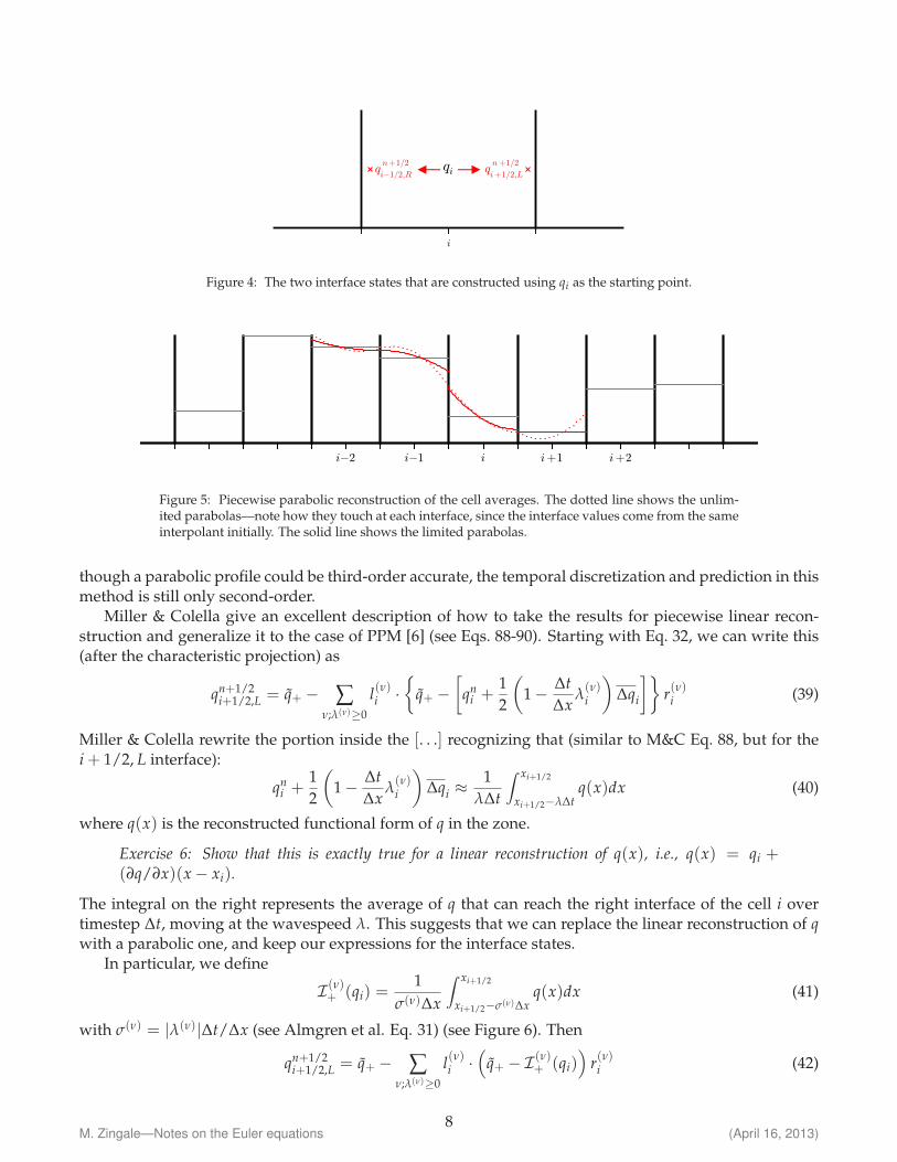
Figure 4: The two interface states that are constructed using qi as the starting point.

ii−1 i+1i−2 i+2

Figure 5: Piecewise parabolic reconstruction of the cell averages. The dotted line shows the unlim-ited parabolas—note how they touch at each interface, since the interface values come from the sameinterpolant initially. The solid line shows the limited parabolas.

though a parabolic profile could be third-order accurate, the temporal discretization and prediction in thismethod is still only second-order.

Miller & Colella give an excellent description of how to take the results for piecewise linear recon-struction and generalize it to the case of PPM [6] (see Eqs. 88-90). Starting with Eq. 32, we can write this(after the characteristic projection) as

qn+1/2i+1/2,L = q+ − ∑

ν;λ(ν)≥0

l(ν)i ·

{q+ −

[qn

i +1

2

(1− ∆t

∆xλ(ν)i

)∆qi

]}r(ν)i (39)

Miller & Colella rewrite the portion inside the [. . .] recognizing that (similar to M&C Eq. 88, but for thei + 1/2, L interface):

qni +

1

2

(1− ∆t

∆xλ(ν)i

)∆qi ≈

1

λ∆t

∫ xi+1/2

xi+1/2−λ∆tq(x)dx (40)

where q(x) is the reconstructed functional form of q in the zone.

Exercise 6: Show that this is exactly true for a linear reconstruction of q(x), i.e., q(x) = qi +(∂q/∂x)(x− xi).

The integral on the right represents the average of q that can reach the right interface of the cell i overtimestep ∆t, moving at the wavespeed λ. This suggests that we can replace the linear reconstruction of qwith a parabolic one, and keep our expressions for the interface states.

In particular, we define

I (ν)+ (qi) =1

σ(ν)∆x

∫ xi+1/2

xi+1/2−σ(ν)∆xq(x)dx (41)

with σ(ν) = |λ(ν)|∆t/∆x (see Almgren et al. Eq. 31) (see Figure 6). Then

qn+1/2i+1/2,L = q+ − ∑

ν;λ(ν)≥0

l(ν)i ·

(q+ − I (ν)+ (qi)

)r(ν)i (42)


(April 16, 2013)

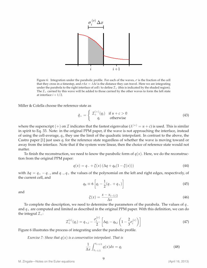
i i+1

σ(ν)i ∆x

Figure 6: Integration under the parabolic profile. For each of the waves, σ is the fraction of the cellthat they cross in a timestep, and σ∆x = λ∆t is the distance they can travel. Here we are integratingunder the parabola to the right interface of cell i to define I+ (this is indicated by the shaded region).The I+ carried by this wave will be added to those carried by the other waves to form the left stateat interface i + 1/2.

Miller & Colella choose the reference state as

q+ =

{I (+)+ (qi) if u + c > 0

qi otherwise(43)

where the superscript (+) on I indicates that the fastest eigenvalue (λ(+) = u + c) is used. This is similarin spirit to Eq. 33. Note: in the original PPM paper, if the wave is not approaching the interface, insteadof using the cell-average, qi, they use the limit of the quadratic interpolant. In contrast to the above, theCastro paper [1] just uses qi for the reference state regardless of whether the wave is moving toward oraway from the interface. Note that if the system were linear, then the choice of reference state would notmatter.

To finish the reconstruction, we need to know the parabolic form of q(x). Here, we do the reconstruc-tion from the original PPM paper:

q(x) = q− + ξ(x) (∆q + q6(1− ξ(x))) (44)

with ∆q = q+ − q−, and q−, q+ the values of the polynomial on the left and right edges, respectively, ofthe current cell, and

q6 ≡ 6

[qi −

1

2(q− + q+)

](45)

and

ξ(x) =x− xi−1/2

∆x(46)

To complete the description, we need to determine the parameters of the parabola. The values of q−and q+ are computed and limited as described in the original PPM paper. With this definition, we can dothe integral I+:

I (ν)+ (qi) = q+,i −σ(ν)i

2

[∆qi − q6,i

(1− 2

3σ(ν)i

)](47)

Figure 6 illustrates the process of integrating under the parabolic profile.

Exercise 7: Show that q(x) is a conservative interpolant. That is

1

∆x

∫ xi+1/2

xi−1/2

q(x)dx = qi (48)


(April 16, 2013)

You can also see that the average over the left half of the zone is qi − 14 ∆q and the average over the right

half of the zone is qi +14 ∆q. This means that there are equal areas between the integral and zone average

on the left and right sides of the zone. This can be seen by looking at Figure 5.

Aside: Note that this characteristic projection of q+ − I (ν)+ is discussed in the original PPMpaper in the paragraph following Eq. 3.5. They do not keep things in this form however, andinstead explicitly multiply out the l · [. . .]r terms to arrive at Eq. 3.6. For example, startingwith Eq. 42, we can write the left velocity state as (leaving off the i subscripts on the vectors):

un+1/2i+1/2,L = u+ −∑

ν

l(ν) · (q+ − I (ν)+ (q)) r(ν)︸︷︷︸only the

u ‘slot′

(49)

(where, as above, the ∼ indicates the reference state). Here the r eigenvector on the end isrepresentative—we only pick the row corresponding to u in the q vector (in our case, thesecond row).

Putting in the eigenvectors and writing out the sum, we have:

un+1/2i+1/2,L = u+ −

(0 − ρ

2c1

2c2

)

ρ+ − I (−)+ (ρ)

u+ − I (−)+ (u)

p+ − I (−)+ (p)

1−c/ρ

c2

−(

1 0 − 1c2

)

ρ+ − I (◦)+ (ρ)

u+ − I (◦)+ (u)

p+ − I (◦)+ (p)

100

−(

0ρ2c

12c2

)

ρ+ − I (+)+ (ρ)

u+ − I (+)+ (u)

p+ − I (+)+ (p)

1c/ρc2

(50)

Here again we show the entire right eigenvector for illustration, but only the element thatcomes into play is drawn in black. This shows that the second term is 0—the contact wave

does not carry a jump in velocity. Multiplying out l(ν) · (q+ − I (ν)+ ) we have:

un+1/2i+1/2,L = u+ −

1

2

[(u+ − I (−)+ (u))− p+ − I (−)+ (p)

C

]− 1

2

[(u+ − I (+)

+ (u)) +p+ − I (+)

+ (p)

C

]

(51)where C is the Lagrangian sound speed (C =

√γpρ). Defining

β+ = − 1

2C

[(u+ − I (+)

+ (u)) +p+ − I (+)

+ (p)

C

](52)

β− = +1

2C

[(u+ − I (−)+ (u))− p+ − I (−)+ (p)

C

](53)

we can write our left state as:

un+1/2i+1/2,L = u+ + C(β+ − β−) (54)

This is Eqs. 3.6 and 3.7 in the PPM paper. Note that in their construction appears to usethe reference state in defining the Lagrangian sound speed (in their β expressions is written


(April 16, 2013)

as C). This may follow from the comment before Eq. 3.6, “modified slightly for the presentapplication”. Similarly, the expressions for ρL and pL can be written out.

Similar expressions can be derived for the right state at the left interface of the zone (qn+1/2i−1/2,R). Here,

the integral under the parabolic reconstruction is done over the region of each wave that can reach the leftinterface over our timestep:

I (ν)− (q) =1

σ(ν)∆x

∫ xi−1/2+σ(ν)∆x

xi−1/2

q(x)dx (55)

The right state at i− 1/2 using zone i data is:

qn+1/2i−1/2,R = q− − ∑

ν;λν≤0

l(ν)i ·

(q− − I (ν)− (qi)

)r(ν)i (56)

where the reference state is now:

q− =

{I (−)− (qi) if u− c < 0

qi otherwise(57)

where the (−) superscript on I indicates that the most negative eigenvalue (λ− = u − c) is used. The

integral I (ν)− (q) can be computed analytically by substituting in the parabolic interpolant, giving:

I (ν)− (qi) = q−,i +σ(ν)i

2

[∆qi + q6,i

(1− 2

3σ(ν)i

)](58)

This is equivalent to Eq. 31b in the Castro paper.

3 The Riemann problem

Once the interface states are created, the Riemann solver is called. This returns the solution at the interface:

qn+1/2i+1/2 = R(qn+1/2

i+1/2,L, qn+1/2i+1/2,R) (59)

Solving the Riemann problem for the Euler equations can be a complex operation, but the generalideas are straightforward. Here we review the basic outline of operations, and refer to Toro [12] for fulldetails on a variety of methods for solving the Riemann problem.

The Riemann problem consists of a left and right state separated by an interface. For the Euler equa-tions, there are three eigenvalues, which are the speeds at which information propagates. Each of thesecorrespond to a wave that will move out from the interface with time, and each wave will carry with it ajump in the characteristic variables. The figure below shows the three waves moving out from the inter-face, separating space into 4 regions, marked: L, L∗, R∗, and R. We typically work in terms of primitivevariables. The states in the L and R regions are simply the left and right input states—the waves have nothad time to reach here, so they are unmodified.

We are interested in the state at the interface. To determine this, we need to determine which regionwe are in. That requires an estimation of the wave speeds. Since these are nonlinear waves, we cannot ingeneral just use the eigenvalues (although some approximate solvers do). Different Riemann solvers willhave different approximations for finding the speeds of the left, center, and right wave. Note the figureshows only one possible configuration for the waves—they can all be on one side of the interface (for allsupersonic waves), or the contact (the middle wave) can be on either side.

Once the wave speeds are known, we look at the sign of the speeds to determine which of the 4 regionsis on the interface. In the ‘star’ region, only ρ jumps across the middle (contact) wave, the pressure and


(April 16, 2013)

ii−1

λ(−) =u−c λ( ◦) =u λ( +) =u+c

L

L ∗ R ∗

R

Figure 7: The wave structure and 4 distinct regions for the Riemann problem. Time can be thoughtof as the vertical axis here, so we see the waves moving outward from the interface.

velocity are constant across that wave (see r(◦)). We determine the state in the star region (ρ∗l , ρ∗r , u∗, p∗)by using the jump conditions for the Euler equations. In general, these differ depending on whether thewaves are shocks or rarefactions. In practice, approximate Riemann solvers often assume one or the other(for example, the two-shock Riemann solver used in [4]). With the wave speeds and the states known in

each region, we can evaluate the state on the interface, qn+1/2i+1/2 .

Recall that a rarefaction involves diverging flow—it spreads out with time. Special considerationneeds to be taken if the rarefaction wave spans the interface (a transonic rarefaction). In this case, mostRiemann solvers interpolate between the left or right state and the appropriate star state.

Then the fluxes are computed from this state as:

Fn+1/2i+1/2 =

ρn+1/2i+1/2 un+1/2

i+1/2

ρn+1/2i+1/2 (u

n+1/2i+1/2 )

2 + pn+1/2i+1/2

un+1/2i+1/2 pn+1/2

i+1/2 /(γ− 1) + 12 ρn+1/2

i+1/2 (un+1/2i+1/2 )

3 + un+1/2i+1/2 pn+1/2

i+1/2

(60)

Note that instead of returning an approximate state at the interface, some Riemann solvers (e.g. theHLL(C) solvers) instead approximate the fluxes directly.

4 Conservative update

Once we have the fluxes, the conservative update is done as

Un+1i = Un

i +∆t

∆x

(Fn+1/2

i−1/2 − Fn+1/2i+1/2

)(61)

The timestep, ∆t is determined by the time it takes for the fastest wave to cross a single zone:

∆t < maxi

∆x

|ui|+ c(62)

5 Multidimensional problems

The multidimensional case is very similar to the multidimensional advection problem. Our system ofequations is now:

Ut + [F(x)(U)]x + [F(y)(U)]y = 0 (63)


(April 16, 2013)

with

U =

ρρuρvρE

F(x)(U) =

ρuρuu + p

ρvuρuE + up

F(y)(U) =

ρvρvu

ρvv + pρvE + vp

(64)

For a directionally-unsplit discretization, we predict the cell-centered quantities to the edges by Taylorexpanding the conservative state, U, in space and time. Now, when replacing the time derivative (∂U/∂t)with the divergence of the fluxes, we gain a transverse flux derivative term. For example, predicting tothe upper x edge of zone i, j, we have:

Un+1/2i+1/2,j,L = Un

i,j +∆x

2

∂U

∂x+

∆t

2

∂U

∂t+ . . . (65)

= Uni,j +

∆x

2

∂U

∂x− ∆t

2

∂F(x)

∂x− ∆t

2

∂F(y)

∂y(66)

= Uni,j +

1

2

[1− ∆t

∆xA(x)(U)

]∆U − ∆t

2

∂F(y)

∂y(67)

where A(x)(U) ≡ ∂F(x)/∂U. We decompose this into a normal state and a transverse flux difference. Adopt-ing the notation from Colella (1990), we use U to denote the normal state:

Un+1/2i+1/2,j,L ≡ Un

i,j +1

2

[1− ∆t

∆xA(x)(U)

]∆U (68)

Un+1/2i+1/2,j,L = Un+1/2

i+1/2,j,L −∆t

2

∂F(y)

∂y(69)

The primitive variable form for this system is

qt + A(x)(q)qx + A(y)(q)qy = 0 (70)

where

q =

ρuvp

A(x)(q) =

u ρ 0 00 u 0 1/ρ0 0 u 00 γp 0 u

A(y)(q) =

v 0 ρ 00 v 0 00 0 v 1/ρ0 0 γp v

(71)

There are now 4 eigenvalues. For A(x)(q), they are u− c, u, u, u + c. If we just look at the system for the xevolution, we see that the transverse velocity (in this case, v) just advects with velocity u, correspondingto the additional eigenvalue.

Exercise 8: Derive the form of A(x)(q) and A(y)(q) and find their left and right eigenvectors.

We note here that Un+1/2i+1/2,j,L is essentially one-dimensional, since only the x-fluxes are involved (through

A(x)(U)). This means that we can compute this term using the one-dimensional techniques developed in§ 2. In particular, Colella (1990) suggest that we switch to primitive variables and compute this as:

Un+1/2i+1/2,j,L = U(qn+1/2

i+1/2,j,L) (72)

Similarly, we consider the system projected along the y-direction to define the normal states on the y-edges, again using the one-dimensional reconstruction on the primitive variables from § 2:

Un+1/2i,j+1/2,L = U(qn+1/2

i,j+1/2,L) (73)


(April 16, 2013)

To compute the full interface state (Eq. 69), we need to include the transverse term. Colella (1990) givestwo different procedures for evaluating the transverse fluxes. The first is to simply use the cell-centeredUi,j (Colella 1990, Eq. 2.13); the second is to use the reconstructed normal states (the U’s) (Eq. 2.15). Inboth cases, we need to solve a transverse Riemann problem to find the true state on the transverse interface.This latter approach is what we prefer. In particular, for computing the full x-interface left state, Un+1/2

i+1/2,j,L,

we need the transverse (y) states, which we define as

UTi,j+1/2 = R(Un+1/2

i,j+1/2,L, Un+1/2i,j+1/2,R) (74)

UTi,j−1/2 = R(Un+1/2

i,j−1/2,L, Un+1/2i,j−1/2,R) (75)

Taken together, the full interface state is now:

Un+1/2i+1/2,j,L = U(qn+1/2

i+1/2,j,L)−∆t

2

F(y)(UTi,j+1/2)− F(y)(UT

i,j−1/2)

∆y(76)

The right state at the i + 1/2 interface can be similarly computed (starting with the data in zone i + 1, jand expanding to the left) as:

Un+1/2i+1/2,j,R = U(qn+1/2

i+1/2,j,R)−∆t

2

F(y)(UTi+1,j+1/2)− F(y)(UT

i+1,j−1/2)

∆y(77)

Note the indices on the transverse states—they are now to the right of the interface (since we are dealingwith the right state).

We then find the x-interface state by solving the Riemann problem normal to our interface:

Un+1/2i+1/2,j = R(Un+1/2

i+1/2,j,L, Un+1/2i+1/2,j,R) (78)

Therefore, construction of the interface states now requires two Riemann solves: a transverse and normalone. The fluxes are then evaluated as:

F(x),n+1/2i+1/2,j = F(x)(Un+1/2

i+1/2,j) (79)

Note, for multi-dimensional problems, in the Riemann solver, the transverse velocities are simply selectedbased on the speed of the contact, giving either the left or right state.

The final conservative update is done as:

Un+1i,j = Un

i,j +∆t

∆x

(F(x),n+1/2i−1/2,j − F

(x),n+1/2i+1/2,j

)+

∆t

∆y

(F(y),n+1/2i,j−1/2 − F

(y),n+1/2i,j+1/2

)(80)

6 Boundary conditions

Boundary conditions are implemented through ghost cells. The following are the most commonly usedboundary conditions. For the expressions below, we use the subscript lo to denote the spatial index of thefirst valid zone in the domain (just inside the left boundary).

• Outflow: the idea here is that the flow should gracefully leave the domain. The simplest form is tosimply give all variables a zero-gradient:

ρlo−1,j

(ρu)lo−1,j

(ρv)lo−1,j

(ρE)lo−1,j

=

ρlo,j

(ρu)lo,j

(ρv)lo,j

(ρE)lo,j

(81)

Note that these boundaries are not perfect. At the boundary, one (or more) of the waves from theRiemann problem can still enter the domain. Only for supersonic flow, do all waves point outward.


(April 16, 2013)

• Reflect: this is appropriate at a solid wall or symmetry plane. All variables are reflected across theboundary, with the normal velocity given the opposite sign. At the x-boundary, the first ghost cellis:

ρlo−1,j

(ρu)lo−1,j

(ρv)lo−1,j

(ρE)lo−1,j

=

ρlo,j

−(ρu)lo,j

(ρv)lo,j

(ρE)lo,j

(82)

The next is:

ρlo−2,j

(ρu)lo−2,j

(ρv)lo−2,j

(ρE)lo−2,j

=

ρlo+1,j

−(ρu)lo+1,j

(ρv)lo+1,j

(ρE)lo+1,j

(83)

and so on . . .

• Inflow: inflow boundary conditions specify the state directly on the boundary. Technically, this stateis on the boundary itself, not the cell-center. This can be accounted for by modifying the stencilsused in the reconstruction near inflow boundaries.

• Hydrostatic: a hydrostatic boundary can be used at the base of an atmosphere to provide the pressuresupport necessary to hold up the atmosphere against gravity while still letting acoustic waves passthrough. An example of this is described in [13].

7 Additional stuff

• Flattening: shocks are self-steepening (this is how we detect them in the Riemann solver—we lookfor converging characteristics). This can cause trouble with the methods here, because the shocksmay become too steep.

Flattening is a procedure to add additional dissipation at shocks, to ensure that they are smearedout over ∼ 2 zones. The flattening procedure is a multi-dimensional operation that looks at thepressure and velocity profiles and returns a coefficient, χ ∈ [0, 1] that multiplies the limited slopes.The convention most sources use is that χ = 1 means no flattening (the slopes are unaltered), whileχ = 0 means complete flattening—the slopes are zeroed, dropping us to a first-order method. Seefor example in Saltzman [10]. Once the flattening coefficient is determined, the interface state isblended with the cell-centered value via:

qn+1/2i+1/2,{L,R} ← (1− χ)qi + χqn+1/2

i+1/2,{L,R} (84)

Note that the flattening algorithm increases the stencil size of piecewise-linear and piecewise-parabolicreconstruction to 4 ghost cells on each side. This is because the flattening procedure itself looks at thepressure 2 zones away, and we need to construct the flattening coefficient in both the first ghost cell(since we need the interface values there) and the second ghost cell (since the flattening procedurelooks at the coefficients in its immediate upwinded neighbor).

• Artificial viscosity: Colella and Woodward argue discuss that behind slow-moving shocks thesemethods can have oscillations. The fix they propose is to use some artificial viscosity—this is addi-tional dissipation that kicks in at shocks. (They argue that flattening alone is not enough).

We use a multidimensional analog of their artificial viscosity ([6], Eq. 4.5) which modifies the fluxes.By design, it only kicks in for converging flows, such that you would find around a shock.


(April 16, 2013)

• Contact steepening: in contrast to shocks, contact waves do not steepen (they are associated withthe middle characteristic wave, and the velocity does not change across that, meaning there cannotbe any convergence). The original PPM paper advocates a contact steepening method to artifi-cially steepen contact waves. While it shows good results in 1-d, it can be problematic in multi-dimensions.

Overall, the community seems split over whether this term should be used. Many people advocatethat if you reach a situation where you think contact steepening may be necessary, it is more likelythat the issue is that you do not have enough resolution.

• Species: for multifluid flows, the Euler equations are augments with continuity equations for each ofthe (chemical or nuclear) species:

∂(ρXk)

∂t+

∂(ρXku)

∂x= 0 (85)

here, Xk are the mass fractions and obey ∑k Xk = 1. Using the continuity equation, we can writethis as an advection equation:

∂Xk

∂t+ u

∂Xk

∂x= 0 (86)

When we now consider our primitive variables: q = (ρ, u, p, Xk), we find

A(q) =

u ρ 0 00 u 1/ρ 00 γp u 00 0 0 u

(87)

There are now 4 eigenvalues, with the new one also being simply u. This says that the species simplyadvect with the flow. The right eigenvectors are now:

r(1) =

1−c/ρ

c2

0

r(2) =

1000

r(3) =

0001

r(4) =

1c/ρc2

0

(88)

corresponding to λ(1) = u − c, λ(2) = u, λ(3) = u, and λ(4) = u + c. We see that for the species,the only non-zero element is for one of the u eigenvectors. This means that Xk only jumps over thismiddle wave. In the Riemann solver then, there is no ‘star’ state for the species, it just jumps acrossthe contact wave.

To add species into the solver, you simply need to reconstruct Xk as described above, find the inter-face values using this new A(q) and associated eigenvectors, solve the Riemann problem, with Xk

on the interface being simply the left or right state depending on the sign of the contact wave speed,and do the conservative update for ρXk using the species flux.

One issue that can arise with species is that even if ∑k Xk = 1 initially, after the update, that may nolonger be true. There are a variety of ways to handle this:

– You can update the species, (ρXk) to the new time and then define the density to be ρ =

∑k(ρXk)—this means that you are not relying on the value of the density from the mass conti-nuity equation itself.

– You can force the interface states of Xk to sum to 1. Because the limiting is non-linear, this iswhere problems can arise. If the interface values of Xk are forced to sum to 1 (by renormalizing),then the updated cell-centered value of Xk will as well. This is the approach discussed in [9].


(April 16, 2013)

– You can design the limiting procedure to preserve the summation property. This approachis sometimes taken in the combustion field. For piecewise linear reconstruction, this can beobtained by computing the limited slopes of all the species, and taking the most restrictiveslope and applying this same slope to all the species.

• Source terms: adding source terms is straightforward. For a system described by

Ut + [F(x)(U)]x + [F(y)(U)]y = H (89)

we predict to the edges in the same fashion as described above, but now when we replace ∂U/∂twith the divergence of the fluxes, we also pick up the source term. This appears as:

Un+1/2i+1/2,j,L = Un

i,j +∆x

2

∂U

∂x+

∆t

2

∂U

∂t+ . . . (90)

= Uni,j +

∆x

2

∂U

∂x− ∆t

2

∂F(x)

∂x− ∆t

2

∂F(y)

∂y+

∆t

2Hi,j (91)

= Uni,j +

1

2

[1− ∆t

∆xA(x)(U)

]∆U − ∆t

2

∂F(y)

∂y+

∆t

2Hi,j (92)

We can compute things as above, but simply add the source term to the U’s and carry it through.

Note that the source here is cell-centered. This expansion is second-order accurate. This is theapproach outlined in Miller & Colella [8].

The original PPM paper does things differently. They construct a parabolic profile of g in each zoneand integrate under that profile to determine the average g carried by each wave to the interface.Finally, they include the gravitational source term in the characteristic projection itself. To see this,write our system in primitive form as:

qt + A(q)qx = G (93)

where G = (0, g, 0)T—i.e. the gravitational source only affects u, not ρ or p. Note that in the PPMpaper, they put G on the lefthand side of the primitive variable equation, so our signs are opposite.Our projections are now:

∑ν;λ(ν)≥0

l(ν) · (q− I (ν)+ (q)− ∆t2 G)r(ν) (94)

for the left state, and

∑ν;λ(ν)≤0

l(ν) · (q− I (ν)− (q)− ∆t2 G)r(ν) (95)

for the right state. Since G is only non-zero for velocity, only the velocity changes. Writing out thesum (and performing the vector products), we get:

un+1/2i+1/2,L = u+ − 1

2

[(u+ − I (−)+ (u)− ∆t

2I (−)+ (g)

)− p+ − I (−)+ (p)

C

]

− 1

2

[(u+ − I (+)

+ (u)− ∆t

2I (+)+ (g)

)+

p+ − I (+)+ (p)

C

](96)

where the only change from Eq. 51 are the I (−)+ (g) and I (+)+ (g) terms.

These differ from the expression in the PPM paper, where ∆tG, not ∆t/2G is used in the projection,however this appears to be a typo. To see this, notice that if both waves are moving toward the

interface, then the source term that is added to the interface state is (∆t/4)(I (−)+ (g) + I (+)+ (g)) for

the left state, which reduces to (∆t/2)g for constant g—this matches the result from the Taylorexpansion above (Eq. 92).


(April 16, 2013)

• General equation of state: The above methods were formulated with a constant gamma equation ofstate. A general equation of state (such as degenerate electrons) requires a more complex method.The classic prescription for extending this methodology is presented by Colella and Glaz [4]. Theyconstruct a thermodynamic index,

γe =p

ρe+ 1 (97)

and derive an evolution equation for γe (C&G, Eq. 26). This evolution equation is used to predict γe

to interfaces, and these interface values of γe are used in the Riemann solver presented there to findthe fluxes through the interface. A different adiabatic index (they call Γ, others call γc) appears inthe definition of the sound speed. They argue that this can be brought to interfaces in a piecewiseconstant fashion while still making the overall method second order, since γc does not explicitlyappear in the fluxes (see the discussion at the top of page 277).

Extending this to an unsplit formulation is not obvious, since the evolution equation for γe is not aconservation law, and it is not obvious what sort of transverse term needs to be incorporated.

Alternately, the Castro paper [1] relies on an idea from an unpublished manuscript by Colella, Glaz,and Ferguson that predicts ρe to edges in addition to ρ, u, and p. Since ρe comes from a conservation-like equation, predicting it to the interface in the unsplit formulation is straightforward. This over-specifies the thermodynamics, but eliminates the need for γe.

With the addition of ρe, our system becomes:

q =

ρupρe

A =

u ρ 0 00 u 1/ρ 00 ρc2 u 00 ρh 0 u

(98)

where h = e + p/ρ is the specific enthalpy. The eigenvalues of this system are:

λ(1) = u− c λ(2) = u λ(3) = u λ(4) = u + c (99)

and the eigenvectors are:

r(1) =

1−c/ρ

c2

h

r(2) =

1000

r(3) =

0001

r(4) =

1c/ρc2

h

(100)

and

l(1) = ( 0 − ρ2c

12c2 0 )

l(2) = ( 1 0 − 1c2 0 )

l(3) = ( 0 0 − hc2 1 )

l(4) = ( 0ρ2c

12c2 0 ) (101)

Remember that the state variables in the q vector are mixed into the other states by l · q. Since alll(ν)’s have 0 in the ρe ‘slot’ (the last position) except for l(3), and the corresponding r(3) is only non-zero in the ρe slot, this means that ρe is not mixed into the other state variables. This is as expected,since ρe is not needed in the system.

Also recall that the jump carried by the wave ν is proportional to r(ν)—since r(1), r(3), and r(4) havenon-zero ρe elements, this means that ρe jumps across these three waves.


(April 16, 2013)

Working through the sum for the (ρe) state, and using a ∼ to denote the reference states, we arriveat:

(ρe)n+1/2i+1/2,L = (ρe) − 1

2

[−ρ

c

(u− I (1)+ (u)

)+

1

c2

(p− I (1)+ (p)

)]h

−[− h

c2

(p− I (3)+ (p)

)+

((ρe)− I (3)+ (ρe)

)]

− 1

2

[ρ

c

(u− I (4)+ (u)

)+

1

c2

(p− I (4)+ (p)

)]h (102)

This is the expression that is found in the Castro code.

All of these methods are designed to avoid EOS calls where possible, since general equations ofstate can be expensive.

• Axisymmetry: it is common to so 2-d axisymmetric models—here the r and z coordinates from acylindrical geometry are modeled. This appears Cartesian, except there is a volume factor implicitin the divergence that must be accounted for. Our system in cylindrical coordinates is:

∂U

∂t+

1

r

∂rF(r)

∂r+

∂F(z)

∂z= 0 (103)

Expanding out the r derivative, we can write this as:

∂U

∂t+

∂F(r)

∂r+

∂F(z)

∂z= −F(r)

r(104)

This latter form is used when predicting the interface states, with the volume source that appearson the right treated as a source term to the interface states (as described above). Once the fluxesare computed, the final update uses the conservative form of the system, with the volume factorsappearing now in the definition of the divergence.

• Defining temperature: although not needed for the pure Euler equations, it is sometimes desirable todefine the temperature for source terms (like reactions) or complex equations of state. The temper-ature can typically be found from the equation of state given the internal energy:

e = E− 1

2u2 (105)

T = T(e, ρ) (106)

Trouble can arise when you are in a region of flow where the kinetic energy dominates (high Machnumber flow). In this case, the e defined via subtraction can become negative due to truncation errorin the evolution of u compared to E. In this instance, one must either impose a floor value for e orfind an alternate method of deriving it.

In [2], an alternate formulation of the Euler equations is proposed. Both the total energy equationand the internal energy equation are evolved in each zone. When the flow is dominated by kineticenergy, then the internal energy from the internal energy evolution equation is used. The cost ofthis is conservation—the internal energy is not a conserved quantity, and switching to it introducesconservation of energy errors.

• Limiting on characteristic variables: some authors (see for example, [11] Eqs. 37, 38) advocate limitingon the characteristic variables rather than the primitive variables. The characteristic slopes for thequantity carried by the wave ν can be found from the primitive variables as:

∆w(ν) = l(ν) · ∆q (107)


(April 16, 2013)

any limiting would then be done to ∆w(ν) and the limited primitive variables would be recoveredas:

∆q = ∑ν

∆w(ν)

r(ν) (108)

(here we use an overline to indicate limiting).

This is attractive because it is more in the spirit of the linear advection equation and the formal-ism that was developed there. A potential downside is that when you limit on the characteristicvariables and convert back to the primitive, the primitive variables may now fall outside of validphysical ranges (for example, negative density).

• New PPM limiters: Recent work [5] has formulated improved limiters for PPM that do not clip theprofiles at extrema. This only changes the limiting process in defining q+ and qi, and does not affectthe subsequent parts of the algorithm.

• 3-d unsplit: The extension of the unsplit methodology to 3-d is described by Saltzman [10]. Thebasic idea is the same as in 2-d, except now additional transverse Riemann solve are needed to fullycouple in the corners.

References

[1] A. S. Almgren, V. E. Beckner, J. B. Bell, M. S. Day, L. H. Howell, C. C. Joggerst, M. J. Lijewski,A. Nonaka, M. Singer, and M. Zingale. CASTRO: A New Compressible Astrophysical Solver. I.Hydrodynamics and Self-gravity. Astrophys J, 715:1221–1238, June 2010.

[2] G. L. Bryan, M. L. Norman, J. M. Stone, R. Cen, and J. P. Ostriker. A piecewise parabolic method forcosmological hydrodynamics. Computer Physics Communications, 89:149–168, August 1995.

[3] P. Colella. Multidimensional upwind methods for hyperbolic conservation laws. Journal of Computa-tional Physics, 87:171–200, March 1990.

[4] P. Colella and H. M. Glaz. Efficient solution algorithms for the Riemann problem for real gases.Journal of Computational Physics, 59:264–289, June 1985.

[5] P. Colella and M. D. Sekora. A limiter for PPM that preserves accuracy at smooth extrema. Journal ofComputational Physics, 227:7069–7076, July 2008.

[6] P. Colella and P. R. Woodward. The Piecewise Parabolic Method (PPM) for Gas-Dynamical Simula-tions. Journal of Computational Physics, 54:174–201, September 1984.

[7] Randall J. LeVeque. Finite-Volume Methods for Hyperbolic Problems. Cambridge University Press, 2002.

[8] G. H. Miller and P. Colella. A Conservative Three-Dimensional Eulerian Method for Coupled Solid-Fluid Shock Capturing. Journal of Computational Physics, 183:26–82, November 2002.

[9] T. Plewa and E. Muller. The consistent multi-fluid advection method. Astron Astrophys, 342:179–191,February 1999.

[10] J. Saltzman. An Unsplit 3D Upwind Method for Hyperbolic Conservation Laws. Journal of Computa-tional Physics, 115:153–168, November 1994.

[11] J. M. Stone, T. A. Gardiner, P. Teuben, J. F. Hawley, and J. B. Simon. Athena: A New Code forAstrophysical MHD. Astrophys J Suppl S, 178:137–177, September 2008.

[12] E. F. Toro. Riemann Solvers and Numerical Methods for Fluid Dynamics. Springer, 1997.


(April 16, 2013)

[13] M. Zingale, L. J. Dursi, J. ZuHone, A. C. Calder, B. Fryxell, T. Plewa, J. W. Truran, A. Caceres, K. Ol-son, P. M. Ricker, K. Riley, R. Rosner, A. Siegel, F. X. Timmes, and N. Vladimirova. Mapping InitialHydrostatic Models in Godunov Codes. Astrophys J Suppl S, 143:539–565, December 2002.


(April 16, 2013)

notes on the euler equations - stony brook...

Documents