Volatility, Intermediaries, and Exchange Rates

Xiang Fang and Yang Liu∗

September 6, 2018

Abstract

This paper studies how time-varying volatility drives exchange rates through financial in-

termediaries’ risk management. We propose a model where currency market participants are

levered intermediaries subject to value-at-risk constraints. Higher volatility translates into tig-

hter financial constraints. Therefore, intermediaries require higher returns to hold foreign as-

sets, and the foreign currency is expected to appreciate. Estimated by the simulated method

of moments, our model quantitatively resolves the Backus-Smith puzzle, the forward premium

puzzle, the exchange rate volatility puzzle, and generate deviations from covered interest rate

parity. Our empirical tests verify model implications that volatility and financial constraint

tightness predict exchange rates.

Keywords: Volatility, Financial Intermediaries, Exchange Rates, Currency Risk Premium,

Value-at-Risk

JEL classification: G15, G20, F31

∗First Version: May 2016. Xiang Fang is at the University of Pennsylvania and Yang Liu is at the University ofHong Kong. Corresponding author (Yang Liu) at: KK1005, University of Hong Kong, Hong Kong. Email: yan-gliu5@hku.hk. Tel: +852-6996-5696. We are grateful to Urban Jermann and Enrique Mendoza for their advice andcomments. We thank Hal Cole, Wei Cui, Alessandro Dovis, Carolin Pflueger (discussant), Karen Lewis, NikolaiRoussanov, Ivan Shaliastovich, Guillaume Vuillemey (discussant), Amir Yaron, Tony Zhang (discussant) and the se-minar and conference participants at 2018 EFA, 2018 Econometric Society China Meeting, 2016 Econometric SocietyEuropean Winter Meeting, 2017 FIRS, University of Pennsylvania, 2017 WFA, and Wharton for valuable commentsand suggestions. All errors are our own.

1

1 Introduction

Exchange rates are puzzling in many aspects. First, exchange rates are disconnected from eco-

nomic fundamentals, especially relative consumption growth rate, which is in sharp contrast to

implications of most international macro-finance models (Backus and Smith, 1993). Second, high-

interest-rate currencies do not depreciate as the uncovered interest parity suggests. On the contrary,

they often appreciate in subsequent periods (Hansen and Hodrick, 1980; Fama, 1984), known as

the “forward premium puzzle”. As a result, excess returns of currency investment can be predicted

by interest rate differentials. Third, it is hard to obtain exchange rate volatility close to data in stan-

dard international macro-finance models (Chari et al., 2002; Brandt et al., 2006). Lastly, covered

interest rate parity, a classic no-arbitrage condition in the currency market, is violated for a decade

after the global financial crisis (Du et al., 2018). In this paper, we attempt to resolve these puzzles

by focusing on the role of leveraged financial intermediaries in exchange rate determination.

Financial intermediaries are major participants in the foreign exchange (FX) market. More than

85% of turnovers in the FX market have financial institutions involved, according to the recent

BIS triennial surveys. Moreover, non-dealer financial institutions account for more than half of

turnovers. With respect to aggregate portfolio holding, the BIS reporting banks hold about half

of the countries’ total external claims and more than 40% of total external liabilities in 21 OECD

countries1.

The recent intermediary asset pricing literature has shown the importance of intermediaries on a

broad class of asset returns (for example, Brunnermeier and Pedersen, 2009; Adrian et al., 2014; He

and Krishnamurthy, 2013; He et al., 2017). It is natural to study exchange rates through the lens of

an intermediary-based model. An essential feature of financial intermediaries is the constraint on

taking leverage. The financial constraint is tightly linked to the volatility in the economy because

of the value-at-risk (VaR) rule adopted by major financial institutions (Adrian and Shin, 2014). The

VaR rule states that the size of the balance sheet shrinks with the rise of volatility in the economy.

1Details will be shown in section 2.

2

In light of the dominance of intermediaries in the FX market and the constraints they are facing, we

introduce these features into an otherwise standard international asset pricing model. The model

has two ex-ante identical countries, home and foreign. Both countries have a continuum of homo-

geneous households and intermediaries. Households only have access to a risk-free money market

account in local intermediaries. Intermediaries take deposits and invest in the local risky asset and

the international bond. Both intermediaries face value-at-risk induced financial constraints, such

that the size of the balance sheet cannot exceed a fraction of their market values (Gertler and Kiyo-

taki, 2010). The fraction increases with the volatility in the economy. In equilibrium, constrained

from taking leverage, intermediaries’ marginal value of assets is higher than that of their liabilities.

Since intermediaries are the only traders on intermediated assets including the local risky asset and

the international bond, they require an excess return on those assets. The exchange rate change

is a large component in international bond returns, so exchange rate dynamics are driven by the

financial constraint. A higher volatility in the home country tightens its intermediaries’ constraint

and increases the difference between the two marginal values, and thus leads to an expected foreign

appreciation.

We estimate the model using the simulated method of moments (SMM), and show that the model

can resolve the four exchange rate puzzles quantitatively. We resolve the Backus-Smith puzzle

by replacing the standard consumption Euler equation with an intermediary Euler equation, so

that consumption and exchange rates are disconnected. As for the forward premium puzzle, when

volatility increases in the home country, its interest rate declines. Meanwhile, because of a higher

excess return required by home intermediaries, there is an expected foreign appreciation. The

exchange rate volatility is closer to data, as the financial constraint amplifies the shocks in the

economy. Finally, the tightened banking regulations after the global financial crises constrain

the intermediaries from making arbitrage in the currency forward market and generate deviations

from covered interest rate parity. Moreover, the model generates the cyclicality of CIP deviations

consistent with empirical evidence documented by Avdjiev et al. (2016). The deviations are large

when home currency is strong, and when volatility is large.

3

We examine additional empirical implications of our model. First, we link exchange rates to the

most direct measure of value-at-risk for currency traders, the exchange rate volatility. We find that

a higher dollar exchange rate volatility predicts an appreciation of foreign currencies, and a higher

currency return borrowing dollar and investing in foreign currencies. Second, as a more direct test

on the channel of intermediaries and financial constraint, we measure the tightness of financial

constraint in the US using the annual growth rate of US financial commercial paper outstanding.

An increase in commercial paper is associated with looser financial conditions. We show that a

higher amount of US financial commercial paper outstanding predicts a foreign depreciation and a

lower foreign currency return. The predictability is preserved after controlling for other predictors

in the literature. Third, when we include the commercial paper and exchange rate volatility in

the standard regression of currency returns on interest rate differentials, the coefficient on interest

rate becomes smaller, and less significant. It indicates that our mechanism is supported by data in

resolving the forward premium puzzle.

Related Literature

A vast literature resolves the exchange rate puzzles in complete market settings. The leading mo-

dels include habit formation (Verdelhan, 2010; Stathopoulos, 2016), long run risks (Colacito and

Croce, 2011, 2013; Bansal and Shaliastovich, 2013), disaster risks (Farhi and Gabaix, 2016), etc.

There are also various attempts to explain these puzzles in incomplete market models, including

Corsetti et al. (2008), Maurer and Tran (2016) and Favilukis et al. (2015). Lustig and Verdelhan

(2016) shows that standard models with only financial market incompleteness cannot resolve mul-

tiple exchange rate puzzles simultaneously. Additional frictions are added into standard models

to account for these puzzles: market segmentation (Alvarez et al., 2002, 2009 and Chien et al.,

2015), nominal rigidity (Chari et al., 2002), search frictions (Bai and Ríos-Rull, 2015), infrequent

portfolio decisions (Bacchetta and Van Wincoop, 2010). Itskhoki and Mukhin (2017) show the key

friction to explaining exchange rate puzzles is the financial shock.

The literature of financial frictions emphasizes several types of constraints faced by capital market

participants. Bernanke et al. (1999), Kiyotaki and Moore (1997), Gertler and Kiyotaki (2010),

4

and Brunnermeier and Sannikov (2014) study the amplification effect of financial frictions on

the macroeconomy. Jermann and Quadrini (2012) uncover that the time variation of financial

constraint is an important source of aggregate fluctuations and financial flows. In the asset pricing

literature, theoretical models show the importance of intermediaries in asset returns (Brunnermeier

and Pedersen, 2009; He and Krishnamurthy, 2013; Li, 2013). Adrian et al. (2014), He et al. (2017),

and Haddad and Muir (2017) find strong supportive evidence for a broad class of asset returns

including stocks, bonds, and more complex securities such as mortgage-backed securities and

derivatives. In international finance, Mendoza (2010) and Perri and Quadrini (2018) show that real

shocks are amplified by financial frictions, leading to financial crisis. Dedola et al. (2013) studies

the transmission of shocks to financial constraints across countries.

Recently, the role of financial intermediation in exchange rate determination is emphasized by

Gabaix and Maggiori (2015). They propose a theory with imperfect intermediation in the interna-

tional financial market. Exchange rates are determined jointly by capital flows and intermediary

balance sheet. Malamud and Schrimpf (2018) develop a theoretical model in which intermediaries

exploit their market power to seek rent, and explain the safe haven properties of exchange rates

and CIP deviation. Our paper is different from them in several aspects. First of all, they provide

theoretical frameworks while we bring the model to data and resolve the four puzzles in a quanti-

tative manner. Second, we highlight the link between stochastic volatility and financial constraint

fluctuations through VaR. Third, their model has a single global intermediary that intermediates

capital flows, while our model studies risk sharing across countries of intermediaries with different

financial constraints. Lastly, we provide supportive empirical evidence on our mechanism. San-

dulescu et al. (2017) use a model-free approach to estimate international SDFs, and show strong

links between model-free international SDFs and intermediary balance sheets as well as volatility.

The rest of the paper is organized as follows. Section 2 lays out some institutional features of

the foreign exchange market and shows the preeminent role of leveraged financial institutions

in exchange rate determination. Section 3 presents the model and section 4 illustrates how this

model can qualitatively resolve the four exchange rate puzzles. In section 5 we estimate our model

5

and show that the model can resolve the four exchange rate puzzles quantitatively. Empirical

implications of the model are tested in section 6. Section 7 concludes the paper.

2 The Relevance of Financial Institutions

This section sketches the basic structure of the foreign exchange market. We show that financial

institutions play a major role in the foreign exchange market, and thus exchange rate determination

2.

The foreign exchange market is the largest financial market in the world, with daily trading volume

exceeding five trillion dollars in 2016, according to the BIS triennial survey. The structure of the

foreign exchange market is two-tier: the inter-dealer market and dealer-customer market. Most

inter-dealer transactions are high-frequency market-making transactions. These high-frequency

transactions are not our considerations, as the half-life of inventory for dealers is only between 1

to 30 minutes, and dealers usually end the day with a small amount of inventories (Bjønnes and

Rime, 2005). There are several exceptions, according to Sager and Taylor (2006), that dealers

take speculative positions in propriety trading with horizons from one day to three months. These

longer horizon speculations are within our consideration in the paper.

Behaviors in the dealer-customer market are important determinants of exchange rates at monthly,

quarterly, or annual frequencies. Main categories of customers include financial customers, cor-

porate customers3, and retail customers4. Financial customers can be divided into two groups:

real money investors and levered investors. Real money investors include mutual funds, pensions

funds, endowments, and so on, which do not take leverage and infrequently adjust their portfolios.

2Though there have been tremendous changes in the foreign exchange market in the recent decades, we describethe common features of the market across time. The new changes include the use of electronic trading systems,the increase of foreign exchange transactions between financial institutions, etc. For more institutional details of theforeign exchange market, see Osler (2008) and King et al. (2011).

3Corporate customers trade for real purposes, such as production, investment, and dividend payout. The size ofcorporate transactions is small relative to financial transactions.

4Retail customers, accounting for a very small fraction, are not studied in this paper.

6

Levered investors include non-dealer commercial banks, hedge funds, and commodity trading ad-

visors, and so on. They take high leverages and actively manage their portfolios.

We show that levered investors account for a substantial portion of turnovers in the FX market in

Table 1 and Figure 1. Table 1 shows the fraction of FX turnovers by different entities from 1998 to

2016. Turnovers associated with nondealer financial institutions keep increasing and rise to 51%

in 2016. Starting from 2013, the BIS triennial survey makes a detailed split of nondealer financial

institutions into nonreporting banks (24%, 22%5), institutional investors (11%, 16%), hedge funds

and, PTFs (11%, 8%), official sector (1%, 1%), and other institutions (6%, 4%). Nonreporting

banks, hedge funds and PTFs, and part of institutional investors are considered as levered investors.

Meanwhile, nonfinancial transactions account for no more than 20% of all turnovers, and it has

been declining in the recent decades. These facts motivate us to focus on the behavior of levered

institutions to study exchange rates.

Besides looking at turnovers in the FX market, we also show the important role of banks in holding

cross-border claims and liabilities using aggregate banking data. Figure 1 plots the time series

weighted average of the ratio of banking claims (liabilities) over total claims (liabilities) from

1977 to 20146. In the late 1970s and early 1980s, banks account for about half of external claims

and 40 percent of external liabilities. This number declined substantially in the late 1990s, to 40

percent (claims) and 30 percent (liabilities) at the trough, possibly due to the global stock market

boom. It rebounded back quickly in the 2000s until the global financial crisis in 2007.

Generally, levered financial intermediaries are constrained in taking leverage, so do the FX market

participants. Speculative positions are constrained for various reasons, such as regulation, risk

management and avoidance of excess risk taking for each trader. Banks in different countries are

subject to the Basel regulatory capital adequacy framework with a minimal risk-weighted capital

ratio of 8 percent and non-risk-weighted leverage ratio of 3 percent. Beyond regulation, FX market

participants face market disciplines in balance sheet management, usually in the form of value-at-5Numbers in 2013 and 2016, respectively.6Countries include Australia, Austria, Belgium, Canada, Denmark, Finland, France, Germany, Greece, Ireland,

Italy, Japan, Netherlands, New Zealand, Norway, Portugal, South Korea, Spain, Sweden, Switzerland, UK, and US.

7

risk (VaR) constraint (Sager and Taylor, 2006). In practice, most intermediaries adopt VaR as

their portfolio risk management model. It calculates the worst possible loss that will not exceed

a given probability over a period. Intermediaries collect data on portfolio positions and market

conditions to calculate their value-at-risk. They use different models to derive time variation in risk,

such as ARCH, GARCH, and exponentially-weighted moving average models. When the Basel

Committee on Banking Supervision allowed commercial banks to use their internal VaR model as

the basis for market risk charge in 1998, the VaR model is widely accepted by the industry (Jorion,

2010). Usually, position limits are imposed on traders to avoid individual excess risk taking (Osler,

2008). Therefore, we argue that the variation in intermediaries’ financial constraint is the distinct

feature of levered institutions that bring us new insights into exchange rate studies.

To sum up, we provide descriptive evidence on the preeminent role financial institutions (banks)

play in the international financial market and their distinct feature of facing leverage constraints.

In the next sections, we incorporate these features into an otherwise standard international asset

pricing model and show these features help us resolve the exchange rate puzzles documented in

the literature.

3 The Model

There are two ex-ante identical countries in the economy, home and foreign, each populated with

a unit measure of households and endowed with a Lucas tree. The home tree delivers good X , and

the foreign tree delivers good Y , both of which are tradable. In both countries, each household

owns an intermediary and sends out a manager to operate it. Households make deposits in local

intermediaries. Intermediaries combine deposits and their own net worth to invest in risky assets.

There are two available risky assets, a claim to the local Lucas tree and an international bond.

Intermediation is imperfect, in the form that the intermediaries in each country face a financial

constraint, whose tightness is determined by the volatility in the local economy. Every period,

a fixed fraction of intermediaries exit the market and rebate back their net worth to their owners,

8

while the same measure of new intermediaries is set up with some initial funds to keep the measure

of intermediaries stationary. The structure of the economy in each country is similar to Gertler and

Kiyotaki (2010).

We describe the behavior of households and intermediaries in detail in the following subsections.

3.1 Households

Households in the home and foreign countries are endowed with a Lucas tree with different goods,

X for home and Y for foreign. They follow cointegrated processes:

logXt+1− logXt = µ + τ(logYt− logXt)+σX ,tεX ,t+1

logYt+1− logY = µ− τ(logYt− logXt)+σY,tεY,t+1 (1)

Volatilities are stochastic, following:

log(σX ,t+1) = (1−ρσ ) log σ̄ +ρσ log(σX ,t)+σσ ηX ,t+1

log(σY,t+1) = (1−ρσ ) log σ̄ +ρσ log(σY,t)+σσ ηY,t+1 (2)

The four shocks follow the standard normal distribution. The two goods aggregate into a consump-

tion basket. The aggregator takes the form of constant elasticity of substitution:

C = [(1−α)Cσ−1

σ

X +αCσ−1

σ

Y ]σ

σ−1 ,C∗ = [(1−α)C∗σ−1

σ

Y +αC∗σ−1

σ

X ]σ

σ−1

CX ,CY are home households’ consumption of X and Y, while variables with an asterisk refer to the

foreign counterpart. Households in the home and foreign countries put different weights on X and

Y with consumption home bias, i.e., α < 12 . σ is the price elasticity of substitution between X and

9

Y. We choose the home composite good as numeraire and define real exchange rate as the price of

foreign composite good Qt . An increase in Qt means a real appreciation of the foreign currency.

In every period, given composite consumption of C, and prices PX ,PY , home households choose

how much X and Y to consume. Home households solve the intratemporal optimization problem:

minCX ,CY

PXCX +PYCY

s.t. : C = [(1−α)Cσ−1

σ

X +αCσ−1

σ

Y ]σ

σ−1

The allocation between X and Y are solved as:

CX =C(PX

PYα

1−α)−σ

PY +PX(PXPY

α

1−α)−σ

,CY =C

PY +PX(PXPY

α

1−α)−σ

(3)

For foreign households, the price of X and Y in foreign consumption basket are PXQ , PY

Q , thus the

solution to foreign intratemporal optimization problem is:

C∗X =C∗(PX

PYα

1−α)−σ Q

PY +PX(PXPY

α

1−α)−σ

,C∗Y =C∗Q

PY +PX(PXPY

α

1−α)−σ

(4)

All households have identical Constant Relative Risk Aversion (CRRA) preferences over their

country-specific consumption basket with risk aversion γ . A fraction αl of the endowment goes

to the households as labor income, while the remaining are capitalized as a risky financial asset.

These financial assets are interpreted broadly as bank loans and other fixed income securities that

are generally intermediated by the financial sector. Households do not hold the risky financial

assets directly. The only financial asset they have access to is a money market account offered by

the local intermediaries, paying one unit of consumption basket risklessly in the subsequent period.

This assumption is consistent with the empirical evidence on households’ limited participation in

the stock market (Vissing-Jørgensen, 2002) and passive portfolio behaviors without rebalancing

10

(Chien et al., 2012). We interpret the labor income component of the endowment as cash flows

received by passive investors. Moreover, this assumption is an extreme case of large efficiency

loss for households to trade risky assets, while intermediaries have a comparative advantage in

investment expertise, as in Brunnermeier and Sannikov (2014).

Households solve a standard intertemporal optimization problem:

maxCt ,Dt

E∞

∑t=0

C1−γ

t −11− γ

s.t. : Ct +Dt = αlPX ,tXt +R f ,t−1Dt−1 +Πt

Dt is the deposit by households into intermediaries at time t, while R f ,t−1Dt−1 is the repayment

from intermediaries of principal and interest. Πt is the net lump-sum payout from the intermedia-

ries that exit the market, which will be specified later. Euler equations hold for households in both

countries:

Etβ (Ct+1

Ct)−γR f ,t = 1, Etβ (

C∗t+1

C∗t)−γR∗f ,t = 1 (5)

3.2 Intermediaries

Each intermediary solves a portfolio choice problem on how much deposit to take, how many

domestic risky asset shares, and how many international bonds to purchase. We exclude the hol-

ding of the foreign tree by intermediaries, since domestic assets dominate foreign assets in most

countries, known as “home equity bias” (Lewis, 1999).

Intermediation is imperfect with a leverage constraint on intermediaries in both countries.

Vt ≥ θt(Ptst +dI,t), V ∗t ≥ θ∗t (P

∗t s∗t +d∗I,t) (6)

Vt ,V ∗t are the market value of an intermediary. Pt ,P∗t are the prices of the Lucas trees denominated

in consumption basket in respective countries. st ,s∗t are the holding shares, and dI,t , d∗I,t are the

11

holding of the international bond. Lower-case variables indicate individual intermediary’s choice,

while upper-case indicate aggregate variables. The international bond pays off riskless return Rb,t

denominated in a half unit of the home composite good and a half unit of the foreign composite

good. We assume this payoff structure to preserve symmetry between the two countries, as in

Heathcote and Perri (2016). When dI,t < 0, home intermediaries are effectively borrowing from

foreign intermediaries to purchase home assets. θt and θ ∗t measures the tightness of leverage

constraint faced by intermediaries, which are linked to the volatility in each economy. We express

θt as a function of the volatility as:

θt = θ0 +θ1log(σX ,t),θ∗t = θ0 +θ1log(σY,t)

These constraints model the distinct feature of intermediaries, the value-at-risk (VaR) constraint,

as we discussed in Section 2. θ0 captures leverage restrictions caused by time-invariant frictions.

θ1log(σX ,t) and θ1log(σY,t) model how the constraint varies with volatility. When volatility in the

economy is higher, the intermediaries’ balance sheets become riskier and they have the incentive to

reduce risk taking. The constraint can be micro-founded within an optimal contracting framework,

such as Adrian and Shin (2014). At the same time, the constraint can also be due to regulation, such

as the Basel III’s minimum risk-weighted capital requirement ratio, non-risk-weighted leverage

ratio requirement, and stress test. Furthermore, borrowing and lending between intermediaries

across borders are settled before repaying the households. Therefore, the VaR constraint is imposed

on the sum of local risky asset and international bond position, even if it is a short position. We

can easily extend the constraint to include different risk weights for the local risky asset and the

international bond position.

From here on, we solve the intermediary problem in the home country. The problem for the foreign

intermediary is exactly identical. The value function of a representative home intermediary can be

12

written recursively as:

Vt(st ,dt ,dI,t) = maxst+1,dt+1,dI,t+1

Etβ (Ct+1

Ct)−γ [(1− p)nt+1 + pVt+1(st+1,dt+1,dI,t+1)]

s.t. : nt+1 +dt+1 ≤ Pt+1st+1 +dI,t+1

θt+1(Pt+1st+1 +dI,t+1)≤Vt+1

V (st ,dt ,dI,t) is the value of the intermediary at the end of period t. The value function is a function

of the holdings of domestic risky asset st , international bond dI,t , and deposit dt . Households

own the intermediaries, so their stochastic discount factor β (Ct+1Ct

)−γ is used to evaluate the cash

flows. In period t + 1, the intermediary exits the market and pays out its net worth nt+1 with

probability 1− p. Otherwise, it continues to operate and choose the holding of st+1,dI,t+1,dt+1,

with continuation value Vt+1(st+1,dt+1,dI,t+1). The first constraint is the balance sheet identity.

The left-hand side is equal to the intermediary’s net worth plus deposit, while the right-hand is the

intermediary’s holding of risky assets. The second constraint is the leverage constraint discussed

before. The dynamics of net worth for a single intermediary is given by:

nt+1 = RS,t+1Ptst +RI,t+1dI,t−R f ,tdt

where RS,t+1 =Pt+1+(1−αl)PX ,t+1Xt+1

Ptis the return on holding domestic risky assets, and RI,t+1 =

1+Qt+11+Qt

Rb,t is the return on holding international bonds. Even though the bond has a noncontingent

return of Rb,t , intermediaries face exchange rate risks.

We guess the value function is linear in all three state variables, and verify later:

Vt = νS,tPtst +νI,tdI,t−νtdt

Assigning the Lagrangian multipliers to the two constraints β (Ct+1Ct

)−γλt+1 and β (Ct+1Ct

)−γψt+1 ,

13

we can obtain the first order conditions:

pνS,t+1 +λt+1−ψt+1(νS,t+1−θt+1) = 0

pνI,t+1 +λt+1−ψt+1(νI,t+1−θt+1) = 0

pνt+1 +λt+1−ψt+1νt+1 = 0

From these three first order conditions, we have the key result:

νS,t = νI,t ≥ νt (7)

νS,t and νI,t are the marginal value of intermediary wealth invested in the domestic risky asset

and the international bond. νt is the marginal cost for the intermediary to take deposits. When

the financial constraint does not bind, all three of them are equal. When the financial constraint

binds, the marginal benefit of investing in the domestic risky asset and the international bond are

identical, both being larger than the marginal cost of taking deposits. The determinant of whether

the financial constraint binds or not is the net worth of the intermediary. If the intermediary has

ample net worth, it will exhaust investment opportunities before hitting the constraint.

We plug back the value function into the Bellman equation, and derive expressions for coefficients:

νI,t = Et

[β (

Ct+1

Ct)−γ(1− p+ pθt+1φ

−1t+1)RS,t+1

]= Et

[β (

Ct+1

Ct)−γ(1− p+ pθtφ

−1t )RI,t+1

](8)

νt = Et

[β (

Ct+1

Ct)−γ(1− p+ pθt+1φ

−1t+1)R f ,t

](9)

φt is the leverage ratio of the home intermediary 7, defined to be:

φt ≡nt

Ptst +dI,t

7More precisely, φt is the ratio of home intermediaries’ net worth over risky position. In our simulated economy,the properties of φt barely change if we define φt =

ntPt st+dIt I(dIt≥0) , where I is an indicator function.

14

Foreign intermediaries face the same problem. The pricing equation of the international bond for

foreign intermediaries is:

ν∗I,t = Et

[β (

C∗t+1

C∗t)−γ(1− p+ pθ

∗t φ∗−1t )RI,t+1

Qt

Qt+1

](10)

3.3 Aggregation

Now that we have specified the problem as well as the optimality conditions for a single interme-

diary. The linearity of the model simplifies aggregation. Due to the representative intermediary

setting, each intermediary has the same optimality conditions and makes the same choices. We can

directly replace individual variables nt ,st ,dt ,dI,t and their foreign counterparts n∗t ,s∗t ,d∗t ,d∗I,t with

the aggregate variables Nt ,St ,Dt ,DI,t ,N∗t ,S∗t ,D

∗t ,D

∗I,t in the optimality conditions.

The net worth dynamics in aggregate is different from the one for a single intermediary, due to

entry and exit. The aggregate dynamics is given by:

Nt+1 = (p+ξ )(RS,t+1PtSt−R f ,tDt +RI,t+1DI,t) (11)

N∗t+1 = (p+ξ )(R∗S,t+1P∗t S∗t −R∗f ,tD∗t +RI,t+1D∗I,t

Qt

Qt+1) (12)

3.4 Equilibrium

Lastly, we have market clearing conditions for good markets and asset markets.

CXt +C∗Xt = Xt , CYt +C∗Yt = Yt , St = S∗t = 1, DI,t +D∗I,tQt = 0 (13)

A competitive equilibrium consists of a sequence of allocations{CXt ,CYt ,C∗Xt ,C∗Yt ,Dt ,D∗t ,Nt ,N∗t ,St ,S∗t ,DI,t ,

D∗I,t ,φt ,φ∗t }, a sequence of prices {R f ,t ,R∗f ,t ,PXt ,PYt ,Pt ,P∗t ,Qt ,Rb,t}, and a sequence of intermedi-

ary valuation {νS,t ,νI,t ,νt ,ν∗S,t ,ν

∗I,t ,ν

∗t } such that:

15

(i) Households in both countries solve their optimization problems;

(ii) Intermediaries in both countries solve their constrained optimization problem;s

(iii) Good markets (X and Y) clear;

(iv) Asset markets (home and foreign deposits, home and foreign risky assets, and the international

bond) clear.

4 Model Mechanisms

4.1 Impulse Response Functions

Figures 2 and 3 report the impulse response functions of different variables in both countries to the

home country’s one-standard-deviation positive endowment shock and volatility shock. Parameters

are estimated and shown in Table 2.

When the home country has a positive endowment shock, the dividend payment of the Lucas tree

increases, and home households’ consumption growth increases. The interaction between inter-

mediary net worth and asset price amplifies the response of return to the home tree. The marginal

value of net worth νI and the marginal cost of borrowing ν both decline, as does the wedge bet-

ween the two. The real risk-free rate in the home country increases slightly. The leverage ratio of

intermediaries increases, because the strengthening of net worth dominates the expansion of their

balance sheets. The endowment shock in the home country is transmitted to the foreign country,

with all foreign variables moving in the same direction but smaller magnitude, as a result of im-

perfect international risk sharing. The mechanism of intermediary balance sheet synchronization

is similar to Dedola et al. (2013). Since both νI and ν∗I decrease, both intermediaries require a

lower expected return on the international bond and Rb decreases. However, νI in the home coun-

try declines more than ν∗I . Consequently, the foreign currency appreciates contemporaneously and

is expected to depreciate. We can also understand the exchange rate movement from the goods

16

market side. An increase in the supply of home good X is accompanied by a contemporaneous

foreign appreciation.

The more interesting channel in our model can be seen in the impulse responses to a one standard

deviation volatility shock. The volatility shock is amplified through the same interaction between

intermediary net worth and asset price illustrated previously. The greater volatility will tighten

home intermediaries’ financial constraints. Since the home intermediaries are not able to take as

much deposit from households, home households’ consumption increases, and home real interest

rate R f decreases. The marginal benefit of net worth νS as well as the marginal cost of borrowing

ν both increase, and so does their difference. The transmission of the shock to the foreign country

is again as previously shown: Foreign variables move in the same direction as home variables

but with a smaller magnitude. Similarly, expected exchange rate change reflects the difference

between home and foreign intermediaries’ valuation of the international bond. Therefore, the

foreign currency is expected to appreciate.

4.2 Asset Prices

In our model, intermediaries play the central role in pricing all the assets. The augmented Euler

equations for intermediaries are key determinants of exchange rates as well as prices for the home

and foreign risky asset. As we show in Section 3.2, the asset pricing equations are equations (8)

and (9).

The stochastic discount factor that prices the domestic tree and the international bond is different

from the one that prices deposits. The difference depends on the wedge between the marginal value

of net worth and the marginal cost of taking deposits, which relies on the tightness of the financial

constraint.

The stochastic discount factor has three components: consumption growth β (Ct+1/Ct)−γ , the sub-

sequent value of the intermediary 1− p+ pθt+1φ−1t+1, and the marginal value of net worth νI,t or the

marginal cost of taking deposits νt . When leverage constraint binds, the leverage constraint can be

17

rewritten as:

θtφ−1t =

Vt

Nt

The additional term 1− p+ pθt+1φ−1t+1 is economically intuitive: With probability 1− p, the inter-

mediary exits the market and pays out its net worth; with probability p, the intermediary continues

to operate, and each dollar remaining in the intermediary generates market value of θt+1φ−1t+1.

4.3 Exchange Rate Puzzles

In this subsection, we review the exchange rate puzzles in the literature and analyze how our model

helps resolve these puzzles.

4.3.1 Backus-Smith Puzzle

Backus and Smith (1993) show that from consumption based Euler equations, exchange rate

change is perfectly correlated with consumption growth differential under the complete market.

To see it more clearly, denote the home stochastic discount factor (SDF) to be Mt+1, and the fo-

reign SDF M∗t+1. Consider the return of home risk-free bond R f ,t , the following equation hold:

Et[Mt+1R f ,t

]= Et

[M∗t+1R f ,t

Qt

Qt+1

]= 1

Qt is the price of foreign goods in terms of home goods. If the financial market is complete, then

the equation holds state by state. Therefore:

∆qt+1 = m∗t+1−mt+1

Lower-case letters are natural logarithms of variables. If we assume a constant relative risk aversion

utility function, we obtain:

∆qt+1 = γ(∆ct+1−∆c∗t+1)

18

Exchange rate change is perfectly correlated with consumption growth differential. Even when the

financial market is incomplete, such as in the models of Heathcote and Perri (2002) and Chari et al.

(2002), the correlation between ∆qt+1 and ∆ct+1−∆c∗t+1 is still close to 1. This is inconsistent with

the weak correlation between exchange rate changes and consumption growth differentials in the

data.

In our model, we have augmented Euler equations for intermediaries in both countries:

Et

[β (

Ct+1

Ct)−γ

(1− p+ pθt+1φ−1t+1)

νI,t

]= Et

[β (

C∗t+1

C∗t)−γ

(1− p+ pθ ∗t+1φ∗−1t+1 )

ν∗I,t

Qt+1

Qt

]

Exchange rate change is linked to consumption growth differential plus two extra terms: the sub-

sequent value of the intermediary, and the relative marginal value of net worth. Therefore, con-

sumption growth is disconnected with exchange rate.

The responses of consumption and exchange rate to endowment and volatility shocks also help us

understand the disconnect. As we show in the impulse response functions in Section 4.1, when

the home country has a positive endowment shock, consumption of home households increases

while the home currency depreciates. On the other hand, when the home country experiences a

positive volatility shock, home consumption increases as well, but the home currency appreciates.

The two forces at play offset each other and generate the weak correlation between consumption

and exchange rate.

4.3.2 Forward Premium Puzzle

Uncovered Interest Rate Parity suggests that when the home country has a higher interest rate than

the foreign country, the home currency is expected to depreciate in the next period so that investing

in home and foreign deliver the same payoffs in expectation. However, this parity condition is

rejected by data (Hansen and Hodrick, 1980; Fama, 1984). Typically, the currency with higher

interest rate tends to further appreciate. This puzzle is also called the “forward premium puzzle”.

In our model, volatility shocks explain the puzzle through intermediaries’ financial constraints. We

19

log-normally approximate the household Euler equation, and obtain:

r f ,t ≈− logβ + γEt∆ct+1−12

γ2Vart∆ct+1

As we show in the impulse response functions in Figure 3, when the home country experiences a

positive volatility shock, the home interest rate is lower for two reasons. First of all, the variance

term 12γ2Vart∆ct+1 is larger and interest rate falls through the precautionary saving effect. Second,

the increased volatility tightens the constraint of home intermediaries. Home households consume

more, thus lower the expected consumption growth Et∆ct+1. The second force also makes foreign

households consume less and increases the foreign interest rate.

As for exchange rates, increased home volatility tightens home intermediaries’ constraints, and

widens the wedge faced by intermediaries. The financial constraint for intermediaries will in turn

affect the international bond and currency market. Home intermediaries require higher expected

returns on the international bonds than foreign intermediaries. Therefore, the foreign currency is

expected to appreciate, even though the foreign interest rate is higher.

With a log-normal approximation, we combine home and foreign intermediaries’ Euler equations

for international bond and deposit, and get:

Et∆qt+1 ≈ (r f ,t− r∗f ,t)+(logνI,t− logνt)− (logν∗I,t− logν

∗t )+ second order terms (14)

Equation (14) links the expected exchange rate change to the intermediaries explicitly. When the

home country experiences a positive volatility shock, home intermediaries are more constrained,

thus logνI,t − logνt > logν∗I,t − logν∗t . If the wedges do not exist, uncovered interest rate parity

holds. In our model, the wedge dominates the interest rate difference in driving exchange rates.

There is a vast literature about the relationship between stochastic volatility and forward premium

puzzle. Backus et al. (2001) show that in a complete market setting with affine linear stochas-

tic discount factors, stochastic volatility is necessary to generate time-varying currency premium.

20

Bansal and Shaliastovich (2013) attributes time variation in currency risk premium to volatility

fluctuations in a structural model. Different from their channel, volatility affects exchange rates

in our model through time-varying financial constraint faced by intermediaries. Therefore, we

are proposing a new mechanism to link volatility to exchange rates that complements the existing

mechanisms.

4.3.3 Exchange Rate Volatility Puzzle

Most international macro-finance models with incomplete financial market cannot generate volatile

exchange rates as in the data. The exchange rate volatility in our model is close to data because

the financial constraints of intermediaries amplify the endowment volatility. As a result, exchange

rates are more volatile than in standard two-country models.

4.3.4 Deviation from Covered Interest Rate Parity

Covered Interest Rate Parity (CIP) is one of the most famous no-arbitrage conditions in finance.

Borrowing in home currency and lending in foreign currency with a currency swap is risk free,

and should yield zero profit. CIP condition holds quite well before the global financial crisis in

2007 (Akram et al., 2008), but is deviated persistently after the crisis (Du et al., 2018). Du et al.

(2018) and Cenedese et al. (2017) illustrate that tightened banking regulation is a key driver of the

CIP deviations. The requirement of the leverage ratio is a non-risk-based constraint imposed on

intermediaries’ balance sheet. Even if CIP arbitrage is riskless, it expands the balance sheet. To

make the expansion subject to the constraint, banks need more capital that is costly. Moreover,

stringent risk-weighted capital requirement and stress tests also increase the opportunity cost of

CIP arbitrage.

This phenomenon is naturally interpretable in our model with intermediaries as arbitrageurs. The

return on foreign risk-free lending through a currency swap is usually called the synthetic home

21

currency rate, denoted as Rcip,t8. In the model, if the intermediaries can conduct CIP arbitrage

without any constraint, then the synthetic home currency rate will have the same Euler equation as

the home currency risk-free rate.

νt = Et

[β (

Ct+1

Ct)−γ(1− p+ pθt+1φ

−1t+1)Rcip,t

]

Therefore, the two rates are equal and CIP holds. After the tightening of regulation, intermediaries

cannot freely trade currency swaps without any constraint. In this case, the marginal value of a

synthetic home currency lending is νI,t , the same as other constrained investments and higher than

the marginal value of deposits νt .

νI,t = Et

[β (

Ct+1

Ct)−γ(1− p+ pθt+1φ

−1t+1)Rcip,t

]

The currency basis rcip,t− r f ,t becomes:

rcip,t− r f ,t = logνI,t− logνt > 0

Hence, constrained intermediaries allow deviations from CIP. In our model, as in the real world,

intermediaries are the major participants in the currency market. Households barely trade currency

swaps, and cannot arbitrage away the currency basis.

Since our model has market segmentation and limits to arbitrage, it is natural for deviations from

CIP to arise. Beyond the existence of the CIP deviations, the model is also able to explain some

of its key cyclical properties. Avdjiev et al. (2016) and Sushko et al. (2017) document that CIP

deviations are large when home currency is strong, and when volatility is large. In the model, CIP

deviations correspond to the tightness of the constraint. When the constraint tightens, home cur-

rency appreciates contemporaneously and is expected to depreciate, as we discussed in the forward8We assume both the synthetic rate and deposit rate are risk free and ignore the risk exposure of CIP arbitrage.

Sushko et al. (2017) explain CIP deviation through counterparty risks of forward contracts. Andersen et al. (2017)consider funding risks and funding value adjustments as an explanation.

22

premium puzzle. Therefore, a stronger home currency is associated with larger CIP deviations. As

for volatility, intuitively, higher volatility tightens the constraint and enlarges the CIP deviations.

5 Quantitative Results

After illustrating the mechanisms to resolve the exchange rate puzzles in the model, we bring the

model to data and match the key facts about exchange rates quantitatively.

5.1 Parameter Estimation

The model is at quarterly frequency. We estimate the model with the simulated method of moments

(SMM). The estimation details are in the Appendix. Benchmark parameter values are reported in

Table 2.

Following the standard practice, we set the time discount factor, labor income share, and risk

aversion at standard values, 0.995, 0.67, and 2 respectively. We assume the average growth rate to

be 0 in order to match the low interest rate level9.

Volatility and of endowment processes are estimated first, using the data in the G7 countries from

1973 to 2015 as in Colacito et al. (2018). Shocks are uncorrelated across countries. The stochastic

volatility processes are the main driving forces of our model. The persistence of the volatility is

0.90, and the volatility of volatility is 0.075. In our model, it is the idiosyncratic volatility that

moves the relative tightness of leverage constraints. Fluctuations in the common component of

volatility do not affect the risk sharing between intermediaries, so they are abstracted from the

model. We impose a weak cointegration relationship between the two endowment processes with

the error correction parameter τ to be 0.0005 to keep the global economy stationary.

9The tension between consumption growth and risk-free rate is a long-standing puzzle (risk-free rate puzzle, Weil,1989). This paper does not attempt to provide any new insight on the resolution of the risk-free rate puzzle. Forexample, introducing recursive utility to separate relative risk aversion and elasticity of intertemporal substitution willmatch the risk-free rate even with an average growth rate of two percent (Bansal and Shaliastovich, 2013).

23

In the SMM, we estimate six parameters, home bias α , trade elasticity σ , survival rate p, ini-

tial funds ξ , the constant and slope of the VaR constraint θ0 and θ1 to match six key moments

about intermediaries and exchange rates: the leverage ratio φ 10, exchange rate volatility sd(∆q),

correlation between exchange rate and consumption growth differential corr(∆q,∆c−∆c∗), OLS

estimates of currency return on interest rate differential βFP and exchange rate change on log vo-

latility βvol, and absolute deviation from CIP rcip− r f . Despite using a new set of exchange rate

related moments in the estimation, our estimates are close to the literature.

The degree of consumption home bias α is as small as 0.043, close to Colacito and Croce (2013).

The elasticity of substitution between the two goods is 0.587, consistent with estimates based on

macro quantities (Stockman and Tesar, 1995; Heathcote and Perri, 2002). The survival rate p and

initial funds rate ξ are 0.964 and 0.003, which implies an average horizon of bankers of a decade.

θ0 is estimated to be 0.376. In Gertler and Kiyotaki (2010), these three parameters are 0.972, 0.003,

and 0.383, very close to the result of our estimation. The slope of θ1 is 0.207, which determines

the relative importance of VaR induced constraint fluctuations on exchange rates.

5.2 Quantitative Results

Table 3 presents the quantitative results of the model.

The first two columns report the moments in the data and in our benchmark model. The upper

panel lists country-specific moments. Among the moments, consumption growth volatility is close

to endowment growth volatility, which is estimated directly from data, and the leverage ratio φ is

chosen as the target moment in our estimation.

Beyond these targets, our benchmark model is able to match the mean and standard deviation

of risk-free rate and the volatility and persistence of the leverage. In terms of the risky asset10We follow the definition by Krishnamurthy and Vissing-Jorgensen (2015) of the “financial sector" of all insti-

tutions supplying short-term debt. These institutions include US-Chartered Depository Institutions, Foreign BankingOffices in the US, Banks in US-Affiliated Areas, Credit Unions, Money Market Mutual Funds, Issuers of Asset-BackedSecurities, Finance Companies, Mortgage Real Estate Investment Trusts, Security Brokers and Dealers, Holding Com-panies and Funding Corporations. Quarterly assets and liabilities data for each type of financial institution are fromthe Flow of Funds.

24

return, we interpret it broadly as intermediated assets, including bank loans and other fixed income

securities, so bond excess returns are preferred proxies to stock excess returns. In the data, the

investment-grade corporate bond holding period return (from Barclays) is 4.01 percent on average,

with a volatility of 5.40 percent. Our model matches the volatility but undershoots risk premium.

However, if we proxy the excess return with the long-term credit spread between Moody’s BAA

corporate bonds and treasury bonds as in Gertler and Kiyotaki (2010), the excess return is 1.78

percent on average, roughly the same magnitude as our model. To highlight the main mechanism,

we abstract from additional features such as habit formation, long-run risks, or disaster risks, to

resolve the equity premium puzzle. The model delivers additional implications on the money

market: the spread between risk-free interbank lending and wholesale funding rmm− r f is equal to

the wedge logνI − logν . Our model implies an average spread of 24 basis points, similar to the

data counterpart of LIBOR-OIS spread.

The lower panel shows that our model can resolve the exchange rate puzzles quantitatively. Ex-

change rate volatility is 8.61 percent, close to the 10 percent in the data. Consumption growth

differential is weakly correlated with exchange rate change, and the regression coefficient of cur-

rency return on interest rate differential is 2.04, greater than unity. Finally, our model generates

an average CIP deviation of 24 basis points as in the data. We note that the magnitude of average

CIP deviation is similar to LIBOR-OIS spread. It is precisely what our model implies: the wedge

logνI,t− logνt is equal to CIP deviation, as well as the spread between risk free interbank lending

and wholesale funding. Moreover, the model generates the cyclicality of CIP deviations consistent

with empirical evidence documented by Avdjiev et al. (2016). The change of CIP basis has a posi-

tive regression coefficient on log currency implied volatility (β∆cip,∆vol =−0.26) 11 and a negative

regression coefficient on the change of exchange rates (β∆cip,∆q = −2.08). Our model can closely

match the size of β∆cip,∆vol and the sign of β∆cip,∆q12. The undershooting of β∆cip,∆q could be a

result of the specialty of the dollar discussed in Avdjiev et al. (2016).

11Our definition of the basis is the negative of theirs, so the coefficient also has an opposite sign.12Since we do not have currency implied volatility in the model, we use the log fundamental volatility σ log(σX ,t).

Assuming unity elasticity between the two volatilities, the model should replicate the regression in the data.

25

To demonstrate the importance of volatility channel through the intermediaries, we turn off the

link between the financial constraint and volatility (θ1 = 0) and report the moments in Column 3.

In this case, the Backus-Smith correlation is as large as 0.70. The forward premium regression

coefficient βFP is extremely large, as in this case the real interest rate barely moves. Exchange

rates are not related to volatility, and the CIP deviation is 69 basis points, much larger than what

we observe in the data. β∆cip,∆vol becomes very small, while the sign of β∆cip,∆q remains negative.

We can conclude that the volatility mechanism through intermediaries goes a long way to explain

the exchange rate puzzles.

Finally, we turn off stochastic volatility completely and report the results in Column 4. The results

are very similar to Column 3, showing that stochastic volatility itself does not play an important

role beyond its effects through the intermediaries.

6 Empirical Implications

Our model provides an exchange rate determination theory through intermediaries, with equation

(14) as the main prediction: the expected exchange rate change is driven by both interest rate

differential and the relative tightness of financial constraints across the two countries. Furthermore,

the financial constraint tightness is driven by the volatility in each country. In this section, we show

that this relation is supported by data.

We first show that a higher dollar exchange rate volatility predicts a foreign appreciation as well

as a higher currency return to borrow the dollar and invest in foreign currencies. As a more direct

test on the channel of intermediaries and financial constraint, we measure the tightness of financial

constraint in the US using the annual growth rate of US financial commercial paper outstanding.

An increase in commercial paper is associated with looser financial constraints. We show that a

higher amount of US commercial paper outstanding predicts a foreign depreciation and a lower

currency return.

26

6.1 Data

We have the spot and forward exchange rate data vis-a-vis dollar for 12 countries: Australia,

Belgium, Canada, Denmark, France, Germany, Italy, Japan, New Zealand, Switzerland, Sweden,

and the UK. The exchange rate data are obtained from Datastream. We also obtain daily spot

exchange rate, compute the realized volatility in each year, and take the average over all these

countries. This measure is the average dollar exchange rate volatility, which is faced by all investors

involved in dollar trade in the FX market. For direct measures of financial constraint, we use

the amount of US outstanding commercial paper for financial business, published by the Federal

Reserve Board. The data spans from January 1991 to December 2015 at monthly frequency. We

use the annual growth rate of commercial paper as our measure. We include several controls of

average forward discounts, US price dividend ratio, US annual growth rate of industrial production,

and exchange rate volatility. The control variables are from National Income and Product Accounts

and CRSP.

6.2 Predictive Regressions with Dollar Exchange Rate Volatility

In this subsection, we examine the relationship between dollar exchange rate volatility, future

dollar exchange rate change, and the return of borrowing dollar and investing in foreign currencies.

We choose the average log dollar exchange rate volatility as a measure of financial constraint

tightness in the US, as it is faced by all investors involved in dollar trade in the FX market.

The results of predictive regressions are shown in Table 4. The upper panel shows results for ex-

change rate changes, and the lower panel shows results for currency returns. Standard errors are

robust to heteroskedasticity, serial autocorrelation, and overlapping observations (Hodrick, 1992).

Univariate regression results in Row 1 to 3 show that a higher dollar exchange rate volatility pre-

dicts a foreign appreciation and a higher currency return. A one percent increase in dollar exchange

rate volatility predicts a 20-basis-points average foreign currency appreciation and 25-basis-points

currency excess returns per annum in horizons of 1 month, 3 months, and 12 months. The results

27

are robust to including various controls, including average forward discount, US price dividend ra-

tio, US industrial production growth. Average forward discount and industrial production growth

are considered drivers of countercyclical currency risk premium (Lustig et al., 2014). Furthermore,

we find that the predictive power of average forward discounts on both exchange rate changes and

currency returns are weakened after controlling for exchange rate volatility.

The upper panel of Figure 4 reports the regression coefficients and confidence intervals of exchange

rate predictability at 3 months horizon for each currency pair. All points estimates are positive and

close to our results in Table 4, and most coefficients are statistically significant.

6.3 Predictive Regressions with US Commercial Paper

In this subsection, we further test the predictive power financial constraint tightness on exchange

rate changes and currency returns. A tighter financial constraint manifests in the money market

first and leads to a smaller amount of commercial paper. Therefore, the financial commercial

paper outstanding is used as a measure of US financial constraint tightness.

Table 5 reports the predictive regression results of commercial paper growth for average dollar

exchange rate and currency returns with different predictive horizons of 1 month, 3 months, and

12 months. The upper panel shows the results for exchange rate changes and the lower panel for

currency returns. From univariate regression results in Row 1 to 3, a one-percent higher commer-

cial paper growth rate in the US predicts a 30 basis point foreign depreciation in the subsequent

month or quarter, and a 20 basis point foreign depreciation in the subsequent year. As for currency

returns, a one percent higher commercial paper growth rate in the US predicts a 38 basis points

lower excess return in the subsequent month or quarter, and a 26 basis points lower excess return in

the subsequent year. In both exchange rate and currency predictive regressions, R2 increases with

predictive horizons.

The predictability of exchange rates and currency returns are also robust to controlling various

variables, including average forward discount, US price dividend ratio, US industrial production

28

growth. In this case, price dividend ratio and industrial production growth rate are considered

credit demand indicators as well. After controlling for these variables, the information contained in

commercial paper mostly comes from the credit supply side, or the tightness of financial constraints

faced by intermediaries. We also find that the predictive power of average forward discounts is

weakened after controlling for commercial paper, while dollar exchange rate volatility becomes

insignificant as well.

In the lower panel of Figure 4, we show the univariate predictive regression coefficients and con-

fidence intervals of exchange rates predictability at 3 months horizon for each currency pair. All

point estimates are negative, and most coefficients are statistically significant.

7 Conclusion

Financial intermediaries are major participants in the foreign exchange market. In light of the

dominance of intermediaries in the FX market and the constraints they are facing, we introduce

these features into an otherwise standard international asset pricing model. An essential feature

of financial intermediaries is the constraint on taking leverage. The financial constraint is tightly

linked to the volatility in the economy because of the value-at-risk (VaR) rule adopted by major

financial institutions.

We estimate the model using the simulated method of moments (SMM), and show that the mo-

del can resolve four exchange rate puzzles quantitatively. We resolve the Backus-Smith puzzle

by replacing the standard consumption Euler equation with an intermediary Euler equation, so that

consumption and exchange rates are disconnected. As for the forward premium puzzle, when vola-

tility increases in the home country, its interest rate declines. Meanwhile, because of higher excess

return required by home intermediaries, there is an expected foreign appreciation. The exchange

rate volatility is closer to data, as the financial constraint amplifies the shocks in the economy.

Tightened banking regulations after the global financial crises constrain the intermediaries from

making arbitrage in the currency forward market and generate deviations from covered interest

29

rate parity. Moreover, the model generates the cyclicality of CIP deviations consistent with em-

pirical evidence. The deviations are large when home currency is strong, and when volatility is

large.

Several model implications are supported by the data. As measures of intermediary financial con-

straints, dollar exchange rate volatility and US financial commercial paper outstanding predict

exchange rate changes and currency returns. When we include the commercial and exchange rate

volatility in the standard regression of currency returns on interest rate differentials, the coefficient

on interest rate becomes smaller and less significant. It indicates that our mechanism is supported

by data in resolving the forward premium puzzle.

30

References

Adrian, T., E. Etula, and T. Muir (2014). Financial intermediaries and the cross-section of asset

returns. The Journal of Finance 69(6), 2557–2596.

Adrian, T. and H. S. Shin (2014). Procyclical leverage and value-at-risk. Review of Financial

Studies 27(2), 373–403.

Akram, Q. F., D. Rime, and L. Sarno (2008). Arbitrage in the foreign exchange market: Turning

on the microscope. Journal of International Economics 76(2), 237–253.

Alvarez, F., A. Atkeson, and P. J. Kehoe (2002). Money, interest rates, and exchange rates with

endogenously segmented markets. Journal of political Economy 110(1), 73–112.

Alvarez, F., A. Atkeson, and P. J. Kehoe (2009). Time-varying risk, interest rates, and exchange

rates in general equilibrium. The Review of Economic Studies 76(3), 851–878.

Andersen, L., D. Duffie, and Y. Song (2017). Funding value adjustments. Technical report, Natio-

nal Bureau of Economic Research.

Avdjiev, S., W. Du, C. Koch, and H. S. Shin (2016). The dollar, bank leverage and the deviation

from covered interest parity.

Bacchetta, P. and E. Van Wincoop (2010). Infrequent portfolio decisions: A solution to the forward

discount puzzle. The American Economic Review 100(3), 870–904.

Backus, D. K., S. Foresi, and C. I. Telmer (2001). Affine term structure models and the forward

premium anomaly. The Journal of Finance 56(1), 279–304.

Backus, D. K. and G. W. Smith (1993). Consumption and real exchange rates in dynamic econo-

mies with non-traded goods. Journal of International Economics 35(3), 297–316.

Bai, Y. and J.-V. Ríos-Rull (2015). Demand shocks and open economy puzzles. The American

Economic Review 105(5), 644–649.

31

Bansal, R. and I. Shaliastovich (2013). A long-run risks explanation of predictability puzzles in

bond and currency markets. Review of Financial Studies 26(1), 1–33.

Bernanke, B. S., M. Gertler, and S. Gilchrist (1999). The financial accelerator in a quantitative

business cycle framework. Handbook of macroeconomics 1, 1341–1393.

Bjønnes, G. H. and D. Rime (2005). Dealer behavior and trading systems in foreign exchange

markets. Journal of Financial Economics 75(3), 571–605.

Brandt, M. W., J. H. Cochrane, and P. Santa-Clara (2006). International risk sharing is better than

you think, or exchange rates are too smooth. Journal of Monetary Economics 53(4), 671–698.

Brunnermeier, M. K. and L. H. Pedersen (2009). Market liquidity and funding liquidity. Review

of Financial studies 22(6), 2201–2238.

Brunnermeier, M. K. and Y. Sannikov (2014). A macroeconomic model with a financial sector.

American Economic Review 104(2), 379–421.

Cenedese, G., P. Della Corte, and T. Wang (2017). Currency mispricing and dealer balance sheets.

Bank of England manuscript.

Chari, V. V., P. J. Kehoe, and E. R. McGrattan (2002). Can sticky price models generate volatile

and persistent real exchange rates? The Review of Economic Studies 69(3), 533–563.

Chien, Y., H. Cole, and H. Lustig (2012). Is the volatility of the market price of risk due to

intermittent portfolio rebalancing? American Economic Review 102(6), 2859–96.

Chien, Y., H. Lustig, K. Naknoi, et al. (2015). Why are exchange rates so smooth? a segmented

asset markets explanation. Technical report.

Colacito, R. and M. M. Croce (2011). Risks for the long-run and the real exchange rate. Journal

of Political Economy 119(1).

32

Colacito, R. and M. M. Croce (2013). International asset pricing with recursive preferences. The

Journal of Finance 68(6), 2651–2686.

Colacito, R., M. M. M. Croce, Y. Liu, and I. Shaliastovich (2018). Volatility risk pass-through.

Corsetti, G., L. Dedola, and S. Leduc (2008). International risk sharing and the transmission of

productivity shocks. The Review of Economic Studies 75(2), 443–473.

Dedola, L., P. Karadi, and G. Lombardo (2013). Global implications of national unconventional

policies. Journal of Monetary Economics 60(1), 66–85.

Du, W., A. Tepper, and A. Verdelhan (2018). Deviations from covered interest rate parity. The

Journal of Finance 73(3), 915–957.

Fama, E. F. (1984). Forward and spot exchange rates. Journal of monetary economics 14(3),

319–338.

Farhi, E. and X. Gabaix (2016). Rare disasters and exchange rates. Quarterly Journal of Econo-

mics 131(1), 1–52. Lead Article.

Favilukis, J., L. Garlappi, and S. Neamati (2015). The carry trade and uncovered interest parity

when markets are incomplete. Available at SSRN.

Fernández-Villaverde, J., J. F. Rubio-Ramírez, and F. Schorfheide (2016). Solution and estimation

methods for dsge models. In Handbook of Macroeconomics, Volume 2, pp. 527–724. Elsevier.

Gabaix, X. and M. Maggiori (2015). International liquidity and exchange rate dynamics. Quarterly

Journal of Economics 130(3).

Gertler, M. and N. Kiyotaki (2010). Financial intermediation and credit policy in business cycle

analysis. Handbook of monetary economics 3(3), 547–599.

Haddad, V. and T. Muir (2017). Do intermediaries matter for aggregate asset prices? Technical

report, Ucla working paper.

33

Hansen, L. P. and R. J. Hodrick (1980). Forward exchange rates as optimal predictors of future

spot rates: An econometric analysis. The Journal of Political Economy, 829–853.

He, Z., B. Kelly, and A. Manela (2017). Intermediary asset pricing: New evidence from many

asset classes. Journal of Financial Economics 126(1), 1–35.

He, Z. and A. Krishnamurthy (2013). Intermediary asset pricing. American Economic Re-

view 103(2), 732–70.

Heathcote, J. and F. Perri (2002). Financial autarky and international business cycles. Journal of

Monetary Economics 49(3), 601–627.

Heathcote, J. and F. Perri (2016). On the desirability of capital controls. IMF Economic Re-

view 64(1), 75–102.

Hodrick, R. J. (1992). Dividend yields and expected stock returns: Alternative procedures for

inference and measurement. The Review of Financial Studies 5(3), 357–386.

Itskhoki, O. and D. Mukhin (2017). Exchange rate disconnect in general equilibrium. Technical

report, National Bureau of Economic Research.

Jermann, U. and V. Quadrini (2012). Macroeconomic effects of financial shocks. American Eco-

nomic Review 102(1), 238–71.

Jorion, P. (2010). Risk management. Annual Review of Financial Economics 2(1), 347–365.

King, M. R., C. L. Osler, and D. Rime (2011). Foreign exchange market structure, players and

evolution. Norges Bank working paper.

Kiyotaki, N. and J. Moore (1997). Credit chains. Journal of Political Economy 105(21), 211–248.

Krishnamurthy, A. and A. Vissing-Jorgensen (2015). The impact of treasury supply on financial

sector lending and stability. Journal of Financial Economics 118(3), 571–600.

34

Lane, P. R. and G. M. Milesi-Ferretti (2007). The external wealth of nations mark ii: Revised

and extended estimates of foreign assets and liabilities, 1970–2004. Journal of international

Economics 73(2), 223–250.

Lewis, K. K. (1999). Trying to explain home bias in equities and consumption. Journal of economic

literature 37(2), 571–608.

Li, K. (2013). Asset pricing with a financial sector. mimeo, HKUST .

Lustig, H., N. Roussanov, and A. Verdelhan (2014). Countercyclical currency risk premia. Journal

of Financial Economics 111(3), 527–553.

Lustig, H. and A. Verdelhan (2016). Does incomplete spanning in international financial markets

help to explain exchange rates? NBER Working Paper.

Malamud, S. and A. Schrimpf (2018). An intermediation-based model of exchange rates.

Maurer, T. A. and N.-K. Tran (2016). Entangled risks in incomplete fx markets.

Mendoza, E. G. (2010). Sudden stops, financial crises, and leverage. The American Economic

Review 100(5), 1941–1966.

Osler, C. L. (2008). Foreign exchange microstructure. Encyclopedia of Complexity and System

Science.

Perri, F. and V. Quadrini (2018). International recessions. American Economic Review 108(4-5),

935–84.

Sager, M. J. and M. P. Taylor (2006). Under the microscope: the structure of the foreign exchange

market. International Journal of Finance & Economics 11(1), 81–95.

Sandulescu, M., F. Trojani, and A. Vedolin (2017). Model-free international sdfs in incomplete

markets.

35

Stathopoulos, A. (2016). Asset prices and risk sharing in open economies. The Review of Financial

Studies 30(2), 363–415.

Stockman, A. C. and L. L. Tesar (1995). Tastes and technology in a two-country model of the

business cycle: Explaining international comovements. The American Economic Review 85(1),

168–185.

Sushko, V., C. E. Borio, R. N. McCauley, and P. McGuire (2017). The failure of covered interest

parity: Fx hedging demand and costly balance sheets.

Verdelhan, A. (2010). A habit-based explanation of the exchange rate risk premium. The Journal

of Finance 65(1), 123–146.

Vissing-Jørgensen, A. (2002). Limited asset market participation and the elasticity of intertemporal

substitution. Journal of Political Economy 110(4).

Weil, P. (1989). The equity premium puzzle and the risk-free rate puzzle. Journal of Monetary

Economics 24(3), 401–421.

36

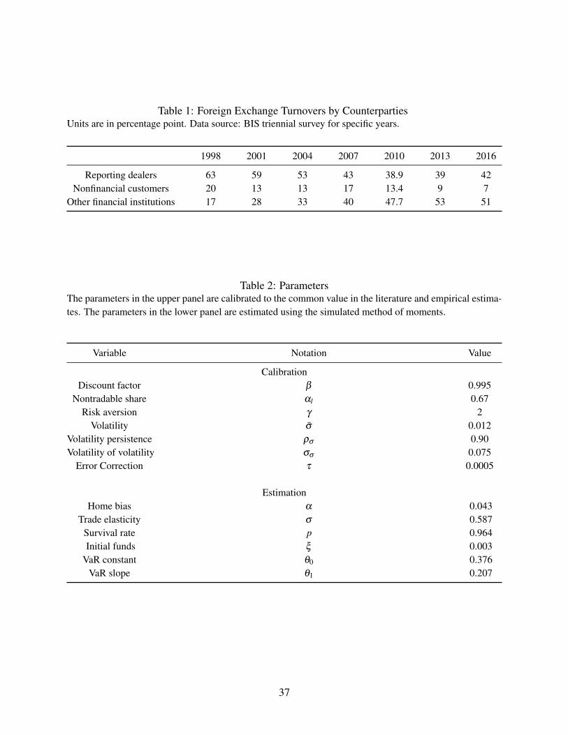
Table 1: Foreign Exchange Turnovers by CounterpartiesUnits are in percentage point. Data source: BIS triennial survey for specific years.

1998 2001 2004 2007 2010 2013 2016

Reporting dealers 63 59 53 43 38.9 39 42Nonfinancial customers 20 13 13 17 13.4 9 7

Other financial institutions 17 28 33 40 47.7 53 51

Table 2: ParametersThe parameters in the upper panel are calibrated to the common value in the literature and empirical estima-tes. The parameters in the lower panel are estimated using the simulated method of moments.

Variable Notation Value

CalibrationDiscount factor β 0.995

Nontradable share αl 0.67Risk aversion γ 2

Volatility σ̄ 0.012Volatility persistence ρσ 0.90Volatility of volatility σσ 0.075

Error Correction τ 0.0005

EstimationHome bias α 0.043

Trade elasticity σ 0.587Survival rate p 0.964Initial funds ξ 0.003

VaR constant θ0 0.376VaR slope θ1 0.207

37

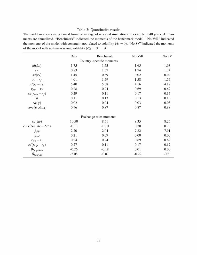
Table 3: Quantitative resultsThe model moments are obtained from the average of repeated simulations of a sample of 40 years. All mo-ments are annualized. “Benchmark” indicated the moments of the benchmark model. “No VaR” indicatedthe moments of the model with constraint not related to volatility (θ1 = 0). “No SV” indicated the momentsof the model with no time-varying volatility (σX = σY = σ̄).

Data Benchmark No VaR No SVCountry -specific moments

sd(∆c) 1.75 1.73 1.65 1.63r f 0.83 1.67 1.74 1.74

sd(r f ) 1.45 0.39 0.02 0.02rs− r f 4.01 1.59 1.58 1.57

sd(rs− r f ) 5.40 5.68 4.16 4.12rmm− r f 0.28 0.24 0.69 0.69

sd(rmm− r f ) 0.29 0.11 0.17 0.17φ 0.11 0.13 0.13 0.13

sd(φ) 0.02 0.04 0.03 0.03corr(φt ,φt−1) 0.96 0.87 0.87 0.88

Exchange rates momentssd(∆q) 10.50 8.61 8.35 8.25

corr(∆q, ∆c−∆c∗) -0.13 -0.10 0.70 0.70βFP 2.20 2.04 7.82 7.91βvol 0.21 0.09 0.00 0.00

rcip− r f 0.24 0.24 0.69 0.69sd(rcip− r f ) 0.27 0.11 0.17 0.17

β∆cip,∆vol -0.26 -0.18 0.01 0.00β∆cip,∆q -2.08 -0.07 -0.22 -0.21

38

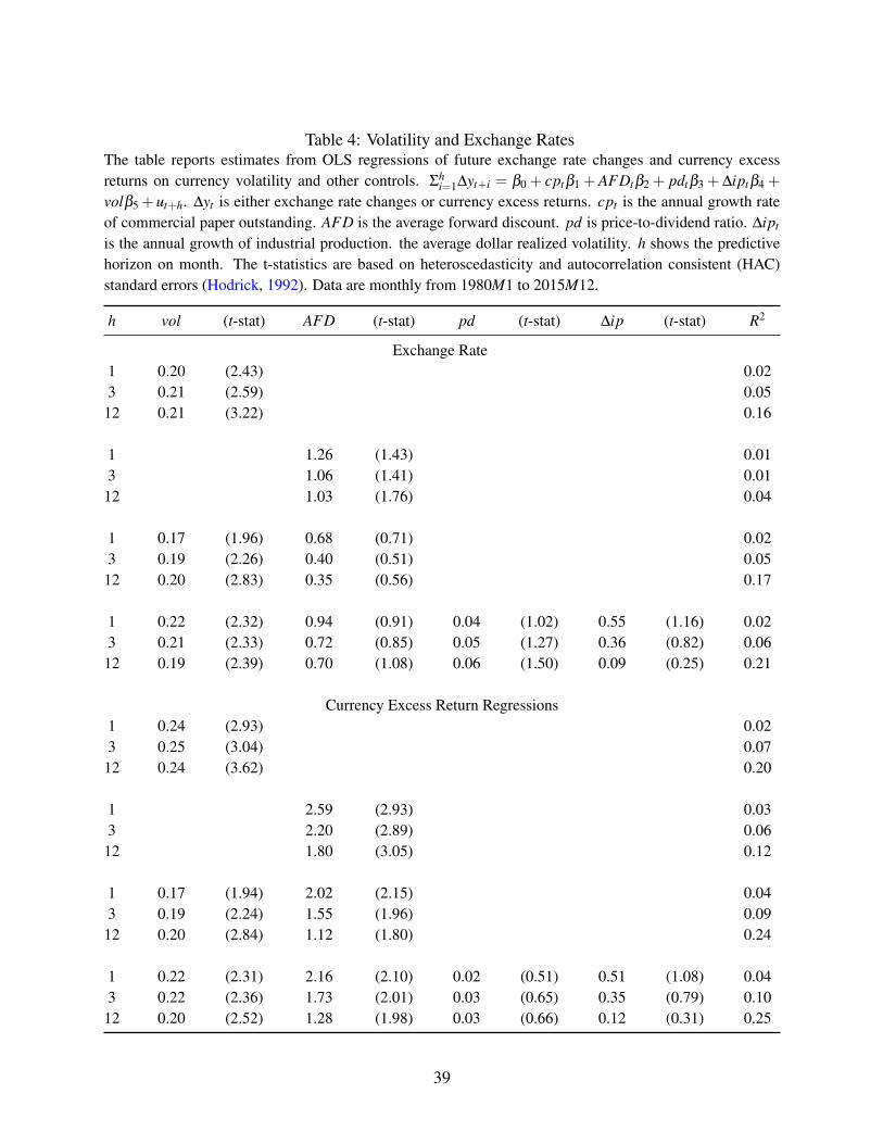
Table 4: Volatility and Exchange RatesThe table reports estimates from OLS regressions of future exchange rate changes and currency excessreturns on currency volatility and other controls. Σh

i=1∆yt+i = β0 + cptβ1 +AFDtβ2 + pdtβ3 +∆iptβ4 +

volβ5 +ut+h. ∆yt is either exchange rate changes or currency excess returns. cpt is the annual growth rateof commercial paper outstanding. AFD is the average forward discount. pd is price-to-dividend ratio. ∆ipt

is the annual growth of industrial production. the average dollar realized volatility. h shows the predictivehorizon on month. The t-statistics are based on heteroscedasticity and autocorrelation consistent (HAC)standard errors (Hodrick, 1992). Data are monthly from 1980M1 to 2015M12.

h vol (t-stat) AFD (t-stat) pd (t-stat) ∆ip (t-stat) R2

Exchange Rate1 0.20 (2.43) 0.023 0.21 (2.59) 0.0512 0.21 (3.22) 0.16

1 1.26 (1.43) 0.013 1.06 (1.41) 0.0112 1.03 (1.76) 0.04

1 0.17 (1.96) 0.68 (0.71) 0.023 0.19 (2.26) 0.40 (0.51) 0.0512 0.20 (2.83) 0.35 (0.56) 0.17

1 0.22 (2.32) 0.94 (0.91) 0.04 (1.02) 0.55 (1.16) 0.023 0.21 (2.33) 0.72 (0.85) 0.05 (1.27) 0.36 (0.82) 0.0612 0.19 (2.39) 0.70 (1.08) 0.06 (1.50) 0.09 (0.25) 0.21

Currency Excess Return Regressions1 0.24 (2.93) 0.023 0.25 (3.04) 0.0712 0.24 (3.62) 0.20

1 2.59 (2.93) 0.033 2.20 (2.89) 0.0612 1.80 (3.05) 0.12

1 0.17 (1.94) 2.02 (2.15) 0.043 0.19 (2.24) 1.55 (1.96) 0.0912 0.20 (2.84) 1.12 (1.80) 0.24

1 0.22 (2.31) 2.16 (2.10) 0.02 (0.51) 0.51 (1.08) 0.043 0.22 (2.36) 1.73 (2.01) 0.03 (0.65) 0.35 (0.79) 0.1012 0.20 (2.52) 1.28 (1.98) 0.03 (0.66) 0.12 (0.31) 0.25

39

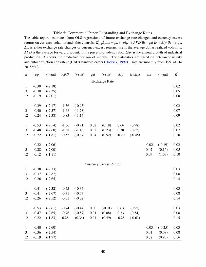
Table 5: Commercial Paper Outstanding and Exchange RatesThe table reports estimates from OLS regressions of future exchange rate changes and currency excessreturns on currency volatility and other controls. Σh

i=1∆yt+i = β0+volβ1+AFDtβ2+ pdtβ3+∆iptβ4+ut+h.∆yt is either exchange rate changes or currency excess returns. vol is the average dollar realized volatility.AFD is the average forward discount. pd is price-to-dividend ratio. ∆ipt is the annual growth of industrialproduction. h shows the predictive horizon of months. The t-statistics are based on heteroscedasticityand autocorrelation consistent (HAC) standard errors (Hodrick, 1992). Data are monthly from 1991M1 to2015M12.

h cp (t-stat) AFD (t-stat) pd (t-stat) ∆ip (t-stat) vol (t-stat) R2

Exchange Rate1 -0.30 (-2.18) 0.023 -0.30 (-2.35) 0.0512 -0.19 (-2.01) 0.08

1 -0.39 (-2.17) -1.56 (-0.95) 0.023 -0.40 (-2.57) -1.68 (-1.28) 0.0712 -0.24 (-2.38) -0.83 (-1.14) 0.09

1 -0.53 (-2.54) -1.66 (-0.91) 0.02 (0.18) 0.66 (0.98) 0.023 -0.48 (-2.60) -1.68 (-1.18) 0.02 (0.23) 0.38 (0.62) 0.0712 -0.22 (-1.81) -0.55 (-0.67) 0.04 (0.52) -0.20 (-0.45) 0.10

1 -0.32 (-2.06) -0.02 (-0.19) 0.023 -0.28 (-2.00) 0.02 (0.16) 0.0512 -0.12 (-1.11) 0.09 (1.03) 0.10

Currency Excess Return1 -0.38 (-2.73) 0.033 -0.37 (-2.87) 0.0812 -0.26 (-2.65) 0.14

1 -0.41 (-2.32) -0.55 (-0.37) 0.033 -0.41 (-2.67) -0.71 (-0.57) 0.0812 -0.26 (-2.52) -0.01 (-0.02) 0.14

1 -0.53 (-2.61) -0.74 (-0.44) 0.00 (-0.01) 0.63 (0.95) 0.033 -0.47 (-2.65) -0.76 (-0.57) 0.01 (0.08) 0.33 (0.54) 0.0812 -0.22 (-1.83) 0.28 (0.34) 0.04 (0.49) -0.28 (-0.63) 0.15

1 -0.40 (-2.60) -0.03 (-0.25) 0.033 -0.36 (-2.54) 0.01 (0.08) 0.0812 -0.19 (-1.77) 0.08 (0.93) 0.16

40

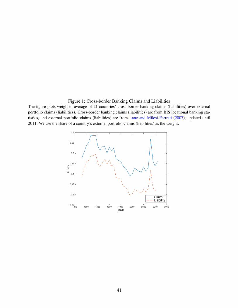
Figure 1: Cross-border Banking Claims and LiabilitiesThe figure plots weighted average of 21 countries’ cross border banking claims (liabilities) over externalportfolio claims (liabilities). Cross-border banking claims (liabilities) are from BIS locational banking sta-tistics, and external portfolio claims (liabilities) are from Lane and Milesi-Ferretti (2007), updated until2011. We use the share of a country’s external portfolio claims (liabilities) as the weight.

year1975 1980 1985 1990 1995 2000 2005 2010 2015

sh

are

0.25

0.3

0.35

0.4

0.45

0.5

0.55

0.6

ClaimLiability

41

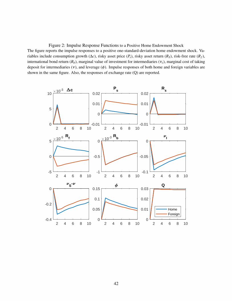
Figure 2: Impulse Response Functions to a Positive Home Endowment ShockThe figure reports the impulse responses to a positive one-standard-deviation home endowment shock. Va-riables include consumption growth (∆c), risky asset price (Ps), risky asset return (RS), risk-free rate (R f ),international bond return (Rb), marginal value of investment for intermediaries (νs), marginal cost of takingdeposit for intermediaries (ν), and leverage (φ ). Impulse responses of both home and foreign variables areshown in the same figure. Also, the responses of exchange rate (Q) are reported.

2 4 6 8 100

5

1010-3 c

2 4 6 8 10-0.01

0

0.01

0.02P

s

2 4 6 8 10-0.01

0

0.01

0.02R

s

2 4 6 8 10-5

0

510-5 R

f

2 4 6 8 10-1

-0.5

010-3 R

b

2 4 6 8 10-0.1

-0.05

0I

2 4 6 8 10-0.4

-0.2

0S-

2 4 6 8 100

0.05

0.1

0.15

2 4 6 8 100

0.01

0.02

0.03Q

HomeForeign

42

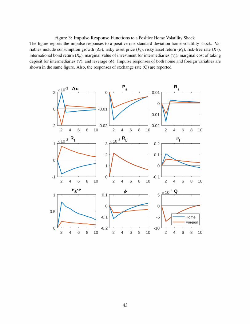
Figure 3: Impulse Response Functions to a Positive Home Volatility ShockThe figure reports the impulse responses to a positive one-standard-deviation home volatility shock. Va-riables include consumption growth (∆c), risky asset price (Ps), risky asset return (RS), risk-free rate (R f ),international bond return (Rb), marginal value of investment for intermediaries (νs), marginal cost of takingdeposit for intermediaries (ν), and leverage (φ ). Impulse responses of both home and foreign variables areshown in the same figure. Also, the responses of exchange rate (Q) are reported.

2 4 6 8 10-2

0

210-3 c

2 4 6 8 10-0.02

-0.01

0P

s

2 4 6 8 10-0.02

-0.01

0

0.01R

s

2 4 6 8 10-1

0

110-3 R

f

2 4 6 8 100

1

2

310-3 R

b

2 4 6 8 10-0.1

0

0.1

0.2I

2 4 6 8 100

0.5

1S-

2 4 6 8 10-0.2

-0.1

0

0.1

2 4 6 8 10-10

-5

0

510-3 Q

HomeForeign

43

Figure 4: Exchange Rate Predictability: Individual CountriesThe Figures presents the univariate regression evidence of predictability of future dollar value by volatilityand growth of commercial paper outstanding. The dependent variables are the log changes in real dollarvalues against individual currencies. The Figure shows the OLS coefficients on exchange rate volatility(upper panel) and commercial paper outstanding (lower panel) and the associated HAC 95% confidenceintervals. Data are monthly from 1980M1 to 2015M12.

-0.2

0

0.2

0.4

0.6

0.8

3-m

onth

fx

Exchange Rate Volatility

AU

S

BE

L

CA

N

FR

A

DE

U

ITA

JPN

NZ

L

NO

R

SW

E

CH

E

GB

R

-1

-0.8

-0.6

-0.4

-0.2

0

0.2

3-m

onth

fx

Commercial Paper

AU

S

BE

L

CA

N

FR

A

DE

U

ITA

JPN

NZ

L

NO

R

SW

E

CH

E

GB

R

44

Appendix: Model Estimation

The equilibrium model is estimate by simulated method of moments (SMM). Estimation methods

are detailed in Fernández-Villaverde et al. (2016).

Denote the moment from data sample by m̂T (Y ) and mode-implied moments E[m̂T (Y )|θ0, M1]

under model M1and parameter θ0. Define the discrepancy

GT (θ |Y ) = m̂T (Y )−E[m̂T (Y )|θ0, M1]

Our estimator θ̂smm minimizes the criterion function of weighted discrepancy

θ̂smm = argminθ GT (θ |Y )′WGT (θ |Y )

Suppose these is a unique θ0 that GT (θ |Y )→ 0 almost surely, then the estimator is consistent.

Our model has six estimated parameters is exactly identified by six moments. The weight matrix

adjust for the difference of the units. When computing the model-implied moments, we simulated

λ = 80 short samples of 40 years data (T = 160).

E[m̂T (Y )|θ0, M1] =1λ

λ

∑i=1

m̂T (Y i|θ0, M1)

A1