volatility forecasting and delta-neutral volatility

Volatility Forecasting and Delta-Neutral Volatility Trading

for DTB Options on the DAX

H.J. Bartels Department of Mathematics and Computer Science

University of Mannheim Seminargebaude -45

D-68131 Mannheim. Germany Tel.: 49-621-1812450 Fax: 49-621-1812506

E-mail: [email protected]

Jian Lu Department of Political Economy

University of Mannheim Seminargebaude A5

D-68131 Mannheim, Germany Tel.: 49-621-1811936 Fax: 49-621-1811931

E-mail: [email protected]

Abstract

One of the most interesting topics in financial time series analysis is the forecasting of the volatility of asset returns. Market practice has found different ways around this problem. One approach derives implied volatilities from actual option prices. Another possibility would be to predict the volatility on the basis of historical asset returns. In recent years the ARCH type models appear to be promising in the mentioned time series context. The optimal choice of an appropriate model for predicting volatility out-of-sample is closely related to the question of how to measure the prediction performance of a model. In our study below, we use four volatility approaches: implied volatility, historical volatility, GARCH( 1 ,l) and EGAR.CH(l,l) volatility forecasts and compare their performance with two option trading strategies. The back-testing includes a time period from July 1995 to July 1997. The methodology we have used in our study offers an opportunity to evaluate the out-of-sample volatility forecast with a convenient metric: the profitability in cumulative profits. ,4s a result it turns out that the performances of the different models are dependent of the used trading strategies and are also depending on filters adopted for the different trading strategies.

Keywords

ARCH models historical volatility, implied volatility.

51

1 Introduction

The interactions between liabilities and assets of life insurance companies are intri- cate and the optimal management of life funds for policyholders is one of the most challenging topics in life insurance business. Since different assets have very different and complex risk characteristics the careful analysis of the used mathematical models is worthwhile. Usually one can not assume, that the values of the model parameters themselves are stationary, hence the way of modelling time series with time dependent parameters deserves special emphasis. In the actuarial context D. Wilkie was one of the first authors which introduced a stochastic asset model for actuarial use (see [ll] and the references therein). The Wilkie approach is mainly intended as a long-term model. But he also used one comparatively simple method to allow for a time varying volatility through what are known as autoregressive conditional heteroscedsstic (ARCH) models of Engle [6]. This sort of model as well as the extensions of this model, for instance the GARCH-models (Generalized ARCH-models) of Bollerslev [4] or the EGARCH-models of Nelson [9] are comparatively easy to investigate and to implement, this is one of the reasons of the popularity of these models in the context of time series analysis.

-4 comprehensive study for an appropriate time-dependent model for all different asset classes relevant in the context of the concrete asset liability management for life insurances in the German market is still pending. One reason could be that the time horizons for the investigations of risk characteristics for different asset classes varies enormously: For the purpose of portfolio insurance of volatile asset classes the speed of adjustment is more important than for long term investment strategies.

The aim of this paper is more modest. We discuss only a special aspect in this context, the volatility forecasting of a certain index on selected German stocks the so called DAX (Deutscher Aktien Index) and applications to options on the DAX, and this is done only for a short time horizon.

Without doubt the use of derivatives is an indispensable tool in the insurance industry especially in life assurance. Derivatives especially options can be used in particular for minimizing the asset-liability mismatch risk, they are important for the management of hedging strategies for special guarantees imbedded in the liability structure of certain products like the index-linked life insurance contracts with an asset value guarantee. Other reasons to use derivatives are for instance: achieving regulatory, accounting or tax efficiencies (altering the apportionment of income and gains) , and the increase of speed of portfolio adjustment (because of the high liquidity in the derivative markets). Hence the mentioned investigations on the DAX volatility can be considered as only one part of a more comprehensive study for a larger model which is needed for applications in the context of the asset liability management in life assurance. In the Black-Scholes world of option pricing volatility is the great unknown. In order to value DTB (Deutsche Termin

52

Borse) options on the DAX the investigation and the estimation of the volatility of the DAX index returns is therefore an obvious task. We concentrate our study to the volatility forecasting. The choice of a particular model for predicting volatility out-of-sample is closely related to the question of how to measure the prediction performance of a model. Here we follow a suggestion in the related study of Noh, Engle and Kane on volatility forecasts on the S&P 500 Index [lo]: In order to test the differences between alternative methods we test the volatility forecasting performance using the potential profitability based on some option trading strategies as a metric. From a practical point of view this method seems plausible, when we evaluate profits from options trading for rival volatility forecasting models and compare them in the same market. So, for the test of the model performance we give the “economic significance” the preference in contrast to the “statistical significance”.

The main results of this paper emanate from the Diplomarbeit of the second named author at Mannheim University in 1998 [7]. The explicit empirical investigations on the DTB DAX option trading were carried out by the second named author during a stay at Commerz Financial Products (CFP) in Frankfurt. The program package S-Plus was used for the statistical part (see section 4 below). This paper is organized as follows. In the next section we present the data description and the trading strategies. Section 3 discusses the volatility forecasting models. Sec- tion 4 presents the evaluation of the extensive empirical results. Finally, section 5 concludes the paper.

2 Data Description and Trading Strategies

2.1 Data Description

We use in our trading strategies options on the DAX (ODAX), which have been traded at the DTB since August 1991. The DAX option has now the largest trading volume of all options at the DTB. ODAX are European style and five different expiry month are always available with a maximum time to maturity of 9 month. There are at least five option series for each expiry date: two are in the money, two are out of the money and one is (approximately) at the money.

The underlying of DTB ODAX is the IBISDAX index. The IBISDAX index includes 30 stocks selected with respect to market capitalisation and turnover. The great advantage of using the IBISDAX index is the fact that it is a performance index which adjusts not only for stock splits and capital changes but also for div- idend payments. The shares are weighted by their share capital and the index is calculated with two decimals.

We use the IBISDAX closing price series (5:00 pm), from July 1991 to July

53

1997, for the volatility estimate and forecasting, and the DTB ODAX settlement price (5:15 pm), from July 1995 to July 1997, as benchmark in our study.

One interesting observation in our study is the following: since the put-call parity is usually not fullfilled, the ODAX settlement price is not exactly caculated with the original IBISDAX closing price. Instead we use an adjusted IBISDAX closing price which results from the put-call parity. A possible explanation for this phenomenon, i.e. the deviation in the put-call parity, is: if good news about the market arrives late in the trading day, then, because of the high liquidity of the index option market, it is likely that the information will be quickly incorporated in options and futures prices. If the information is not fully reflected in the cash- market index by the close of trading because some component stocks do not trade before the close, the observed-index level is lower than it should be, and the implied volatility of the call is higher than it should be. On the following day, when all stocks in the index have traded and reacted to the previous day’s news, the observed-index level catches up, and the implied volatility of the call is reduced. In this case index puts will have a low implied volatility at the close, and the volatility will recover the next day. Similarly, if bad news arrives late in the trading day, the price of index puts is quickly bid up. If not all stocks in the index are traded by the close of trading, the observed closing-index level is higher than it should be. The implied volatility of puts is higher than it should be, and on the following day the implied volatility of puts is reduced.

From the data sets described above, we collect data for (approximately) at the money straddle with maturity between 15 and 45 days, i.e., for each day, we select the straddle settlements price whose strike price is closest to the index level.

For the risk-free rate of interest in option pricing we have used the overnight FIBOR (Frankfurt Inter Bank Offer Rate), 1 month FIBOR, and 2 month FI- BOR. The present value are computed using log-linear interpolation with respect to maturity.

2.2 Trading Strategy

The aim of this study is to evaluate the profitability of applying different models to a pure volatility trading strategy. As we know that the closest at the money straddles are approximately delta neutral (see for example [S]) , i.e. the price changes of straddle with respect to the market movement can be tolerated, it is appropriate to use them to a pure volatility trading strategy. The straddle position will also have sensitivities with respect to the interest rate (rho) and the time to maturity (theta). These sensitivities are ignored in our study, because the positions in our strategy are not longer than two days as described below.

The basic idea for the delta-neutral trading strategy is: during the sample period, on each day, we apply a particular forecasting method to get a volatil-

54

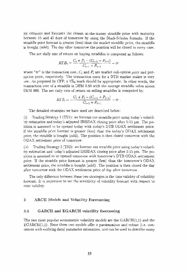
ity estimate and forecasts the closest at-the-money straddle price with maturity between 15 and 45 days of tomorrow by using the Black-Scholes formula. If the straddle price forecast is greater (less) than the market straddle price, the straddle is bought (sold). The day after tomorrow the position will be closed in every case.

The net daily rate of return on buying straddles is computed as follows:

RTB t

= ct + 6 - (Ct-1 + 6-l) _ tr ct-1 + pt-l

where “tr” is the transaction cost, C, and Pt are market call-option price and put- option price, respectively. The transaction costs for a DTB market maker is very low. As proposed by CFP, a l%, mark should be appropriate. In other words, the transaction cost of a straddle is DEM 0.80 with the average straddle value about DEM 800. The net daily rate of return on selling straddles is computed by:

RTS t = -ct + 8 - (G-1 + C-1) G-1 + 8-l - tr

The detailed strategies we have used are described below:

(i) Trading Strategy 1 (TSl): we forecast our straddle price using today’s volatility estimation and today’s adjusted IBISDAX closing price after 5:15 pm. The position is assumed to be opened today with today’s DTB ODAX settlement price: If the straddle price forecast is greater (less) than the today’s ODAX settlement price, the straddle is bought (sold). The position is then closed tomorrow with the ODAX settlement price of tomorrow.

(ii) Trading Strategy 2 (TS2): we forecast our straddle price using today’s volatility estimation and today’s adjusted IBISDAX closing price after 5:15 pm. The position is assumed to be opened tomorrow with tomorrow’s DTB ODAX settlement price: If the straddle price forecast is greater (less) than the tomorrow’s ODAX settlement price, the straddle is bought (sold). The position is then closed the day after tomorrow with the ODAX settlement price of day after tomorrow.

The only difference between these two strategies is the time validity of volatility forecast. It is important to see the sensitivity of volatility forecast with respect to time validity.

3 ARCH Models and Volatility Forecasting

3.1 GARCH and EGARCH volatility forecasting

The two most popular econometric volatility models are the GARCH(l,l) and the EGARCH(1,l). Since these two models offer a parsimonious and robust (i.e. consistent with outlying data) parameter estimation, and can be used to describe many

55

financial time series, they established themselves as a kind of “industry standar” over the years.

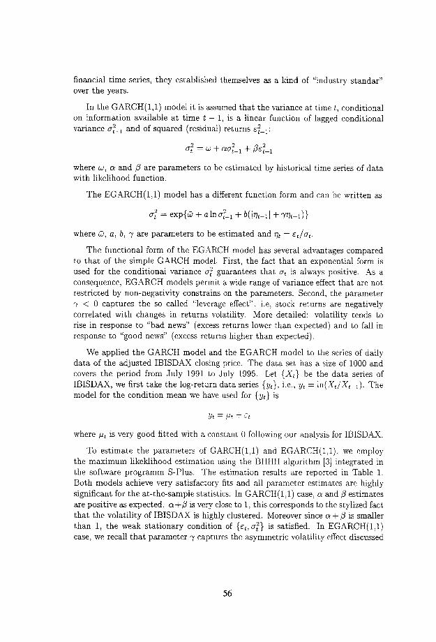
In the GARCH(l,l) model it is assumed that the variance at time t, conditional on information available at time t - 1, is a linear function of lagged conditional

2 variance gt-i and of squared (residual) returns &:

UP = w + a& + p&f-,

where w, LY and ,0 are parameters to be estimated by historical time series of data with likelihood function.

The EGARCH(l,l) model has a different function form and can be written as

uf = exp{G + aIn&, + b(/qt-iI +-m--1)}

where 6; a, b, y are parameters to be estimated and Q = st/gt.

The functional form of the EGARCH model has several advantages compared to that of the simple GARCH model. First, the fact that an exponential form is used for the conditional variance u2 t guarantees that CT~ is always positive. -4s a consequence, EGARCH models permit a wide range of variance effect that are not restricted by non-negativity constrains on the parameters. Second, the parameter n/ < 0 captures the so called “leverage effect”, i.e, stock returns are negatively correlated with changes in returns volatility. More detailed: volatility tends to rise in response to “bad news” (excess returns lower than expected) and to fall in response to “good news” (excess returns higher than expected).

We applied the GARCH model and the EGARCH model to the series of daily data of the adjusted IBISDAX closing price. The data set has a size of 1000 and covers the period from July 1991 to July 1995. Let {X,} be the data series of IBISDAX, we first take the log-return data series {yl}, i.e., yt = ln(Xt/Xt-i). The model for the condition mean we have used for {yt} is

l/t = Pt + Et

where pLt is very good fitted with a constant 0 following our analysis for IBISDA,X.

To estimate the parameters of GARCH(l,l) and EGAR.CH(l,l), we employ the maximum likeklihood estimation using the BHHH algorithm [3] integrated in the software programm S-Plus. The estimation results are reported in Table 1. Both models achieve very satisfactory fits and all parameter estimates are highly significant for the at-the-sample statistics. In GARCH(l,l) case, QI and p estimates are positive as expected. cu+/3 is very close to 1, this corresponds to the stylized fact that the volatility of IBISDAX is highly clustered. Moreover since LY + @ is smaller than 1, the weak stationary condition of {st,crz} is satisfied. In EGARCH(1,l) case, we recall that parameter y captures the asymmetric volatility effect discussed

56

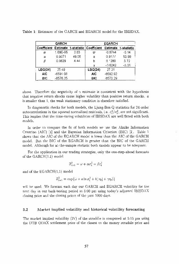
Table 1: Estimates of the GARCH and EGARCH model for the IBISDAX

GARCH EGARCH Coefficient Estimate t-statistic Coefficient Estimate t-statistic

al l.O9E-05 3 63 w -0.8744 -5 14

I 0.9071 0.0629 49.06 4 44 a b 0 0.1280 9177 53.99 3 72 Y -0 6242 -3.00

LBQ(2d) 25.49 LBP(24) 27.31 AK -6591 08 AK -6592 92 BIC -6576.35 BIC -6573.29

above. Therefore the negativity of y estimate is consistent with the hypothesis that negative return shocks cause higher volatility than positive return shocks. a is smaller than 1, the weak stationary condition is therefore satisfied.

In diagonostic checks for both models, the Ljung-Box-Q statistics for 24 order autocorrelations in the squared normalized residuals, i.e. &f/of, are not significant. This implies that the time-varing volatilities of IBISDAX are well fitted with both models.

In order to compare the fit of both models we use the Akaike Information Criterion (AIC) [I] and the Bayesian Information Criterion (BIC) [2]. Table 1 shows that the AIC of the EG.4RCH model is lower than the .4IC of the GXRCH model. But the BIC of the EGARCH is greater than the BIC of the GARCH model. Although for at-the-sample statistic both models appear to be adequate.

For the application in our trading strategies, only the one-step-ahead forecasts of the GARCH(1.1) model

-2 Ot+1 = w + cm,” + ,s?E;

and of the EGARCH(l,l) model

2 t+l = exp{G + alno: + b(lvtl + wt)}

will be used. We forecast each day our GARCH and EGARCH volatility for the next day in our back-testing period at 5:00 pm using today’s adjusted IBISDAX closing price and the closing prices of the past 1000 days.

3.2 Market implied volatility and historical volatility forecasting

The market implied volatility (IV) of the straddle is computed at 5:15 pm using the DTB ODAX settlement price of the closest to the money straddle price and

57

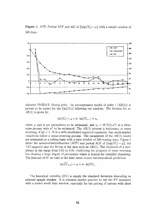
Figure 1: ACF, Partial ACF and AIC of {log(lVt) - ,u} with a sample window of

200 days.

180

t PartiP, ACF

160

80 -- - - . -__--_--- - - - - - - - - - - - - - - - - - - - - - - - -

60

adjusted IBISDAX closing price. i\n autoregressive model of order 1 (AR(l)) is proved to be suited for the {ln(lVt)} following our analysis. The formula for an AR(l) is given by:

In(W) = p + 4. ln(lGit-i) + zt .

where p and 4 are parameters to be estimated, and .zt N WN(O,a’) is a white noise process with cr2 to be estimated. The AR(l) process is stationary, or mean reverting, if 141 < 1. It is a well-established empirical regularity that stock-market volatilities follow a mean-reverting process. The parameters of the AR(l) model are estimated on a rolling basis with a data window of 200 trading days. Figure 1 shows the autocorrelationfunction (ACF) and partial ACF of {log(l&) - p}, the r-\IC supports also the fitting of the data with an AR(l). The estimates of (b were always in the range from 0.85 to 0.95, confirming the property of mean reversion but showing a large degree of persistence which is typical for volatility clustering. The forecast of IV we take is the least mean square one-step-ahead prediction

ln(lG,+i) = p + +$.ln(1&)

The historical volatility (HV) is simply the standard deviation depending on selected sample window. It is common market practice to use the HV estimator with a rather small data window, especially for the pricing of options with short

58

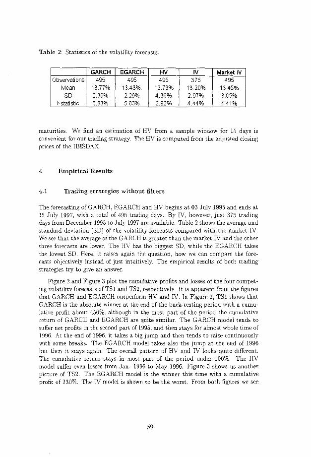
Table 2: Statistics of the volatility forecasts.

GARCH EGARCH HV IV Market IV Observations 495 495 495 375 495

Mean 13.77% 13 43% 12.73% 13 20% 13 45% SD 2.36% 2.29% 4.36% 2 97% 3.05%

t-statistic 5.83% 5 83% 2.92% 444% 441%

maturities. We find an estimation of HV from a sample window for 15 days is convenient for our trading strategy. The HV is computed from the adjusted closing prices of the IBISDAX.

4 Empirical Results

4.1 Trading strategies without filters

The forecasting of GXRCH, EGARCH and HV begins at 03 July 1995 and ends at 15 July 1997, with a total of 495 trading days. By IV, however, just 375 trading days from December 1995 to July 1997 are available. Table 2 shows the average and standard deviation (SD) of the volatility forecasts compared with the market IV. We see that the average of the GARCH is greater than the market IV and the other three forecasts are lower. The HV has the biggest SD, while the EGARCH takes the lowest SD. Here, it raises again the question, how we can compare the forecasts objectively instead of just intuitively. The empirical results of both trading strategies try to give an answer.

Figure 2 and Figure 3 plot the cumulative profits and losses of the four competing volatility forecasts of TSl and TS2, respectively. It is apparent from the figures that GARCH and EGARCH outperform HV and IV. In Figure 2, TSl shows that GARCH is the absolute winner at the end of the back-testing period with a cumulative profit about 450%. although in the most part of the period the cumulative return of GARCH and EGARCH are quite similar. The GARCH model tends to suffer net profits in the second part of 1995, and then stays for almost whole time of 1996. At the end of 1996, it takes a big jump and then tends to raise continuously with some breaks. The EGARCH model takes also the jump at the end of 1996 but then it stays again. The overall pattern of HV and IV looks quite different. The cumulative return stays in most part of the period under 100%. The HV model suffer even losses from Jan. 1996 to May 1996. Figure 3 shows us another picture of TS2. The EGARCH model is the winner this time with a cumulative profit of 230%. The IV model is shown to be the worst. From both figures we see

59

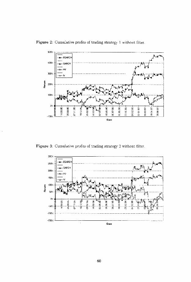
Figure 2: Cumulative profits of trading strategy 1 without filter

II - - EGARCH


II- I I 250%

tl

- EGARCH - I-.-----......_________^_______________ I...;n: _____ p.pJ

E 100% I d 50%

4 4

60

that ARCH models and the HV and IV models generate different trading signals at some “big points” which is reflected in the different developments of cumulative returns.

Moreover we find the EGARCH and HV models are quite stable for both trading strategies, while GARCH and IV models are very sensitive to different strategies. A possible explanation for this phenomenon is: volatility forecasts of different models have a different time validity. The time difference between volatility forecasting and position closing by TSl is about one day, while it takes two days by TS2. Although GARCH model has the best performance by TSl, it seems that the time validity of the GARCH forecast is shorter. In comparison, the volatility forecast of EGARCH tends to have a longer time validity and performs similarly in both strategies.

4.2 Trading strategies with different filters

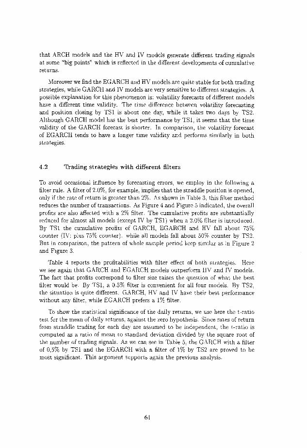
To avoid occasional influence by forecasting errors, we employ in the following a filter rule. A filter of 2.0%, for example, implies that the straddle position is opened, only if the rate of return is greater than 2%. As shown in Table 3, this filter method reduces the number of transactions. As Figure 4 and Figure 5 indicated, the overall profits are also affected with a 2% filter. The cumulative profits are substantially reduced for almost all models (except IV by TSl) when a 2.0% filter is introduced. By TSl the cumulative profits of GARCH, EGARCH and HV fall about 75% counter (IV: plus 75% counter). while all models fall about 50% counter by TS2. But in comparison, the pattern of whole sample period keep similar as in Figure 2 and Figure 3.

Table 4 reports the profitabilities with filter effect of both strategies. Here we see again that GARCH and EGARCH models outperform HV and IV models. The fact that profits correspond to filter size raises the question of what the best filter would be. By TSl, a 0.5% filter is convenient for all four models. By TS2, the situation is quite different. GARCH, HV and IV have their best performance without any filter, while EGARCH prefers a 1% filter.

To show the statistical significance of the daily returns, we use here the t-ratio test for the mean of daily returns, against the zero hypothesis. Since rates of return from straddle trading for each day are assumed to be independent, the t-ratio is computed as a ratio of mean to standard deviation divided by the square root of the number of trading signals. As we can see in Table 5, the GARCH with a filter of 0,5Y0 by TSl and the EGARCH with a filter of 1% by TS2 are proved to be most significant. This argument supports again the previous analysis.

61

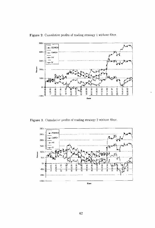
Figure 2: Cumulative profits of trading strategy 1 without filter.


300%

250%

200%

150%

07.

-50%

62

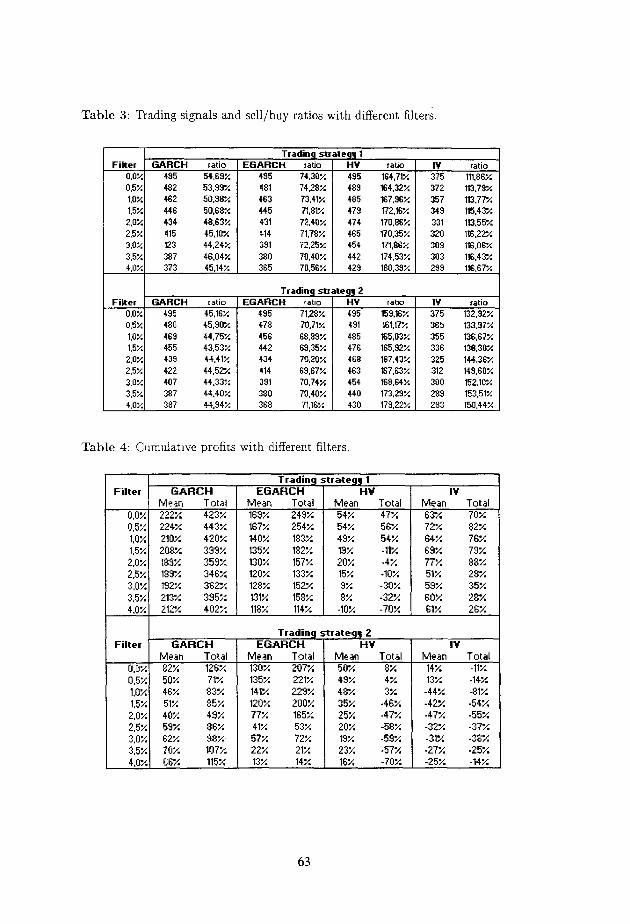
Table 3: Trading signals and sell/buy ratios with different filters

Trading stratcgg 1 Filter GARCH ratio EGARCH ratio HV ratio IV ratio

0.0% 495 54.69% 495 74.30% 495 164.71% 375 111.86% 0.5% 482 53.39% 481 74.282 489 164.32% 372 113.73% 1.0% 462 50.38% 463 73.41% 485 167.36% 357 113.772 1.5% 446 50.68% 445 71.81% 473 172.16x 349 H5.432

2.0% 434 48.63% 431 72.40% 474 170.86% 331 113.55x 2.5% 415 45.10% 414 71.782 465 170.35% 320 116.22% 3.0% 123 44.24% 391 72.252 454 171,86% 309 116.08% 3.5% 387 46.04% 380 70.40% 442 174.532 303 116.43% 4.0% 373 45.14% 365 70.56% 429 190.33% 299 116.67%

Tradinq stl Filter GARCH ratio EGARCH ratio

0.0% 495 45.16% 495 71.28x 0.5% 480 45.30% 478 70.71% 1.0% 469 44.75% 456 68.83% 1.5% 455 43.53% 442 69.35%

2.0% 439 44.41% 434 70.20% 2.5% 422 44.52% 414 63.67% 3.0% 407 44.33% 331 70.74% 3.5% 387 44.40% 380 iO.40% 4.0% 387 44.94% 368 71.16::

Table 4: Cumulative profits with different filters.

eg,2 HV ratio 495 159.162 491 161.17% 485 165.03% 476 165.92% 468 167.43% 463 167,632 454 168.64% 440 173.23% 430 173.222

Tradin EGARCH

0.52 224% 443% 1.0% 210% 420% ” : 1.5% 208% 333%

2.0% 185x 359% c 2.5% 189% 346% 3.0% 192% 362% 3,5% 213% 395% 4.0% 2lzz 403" LX.

Mean Total 163% 2492 167% 254% 140% 183% 135% 182% 130% 1572 120% 133% 128% 152% 131% 158% 118% 114%

Tradinq EGARCH

Mean Total 130% 207% 135% 221% 14w 229% 120% 200% 77% 165% 41% 53'/ 57% 72z 22% 21% 13% 14%

50% 71% 46% 83% 51% 85% 40% 19% 59% 86% 622 38% 70% 107% 66% 115%

rate 1

Mean Total 54% 47% 54% 56% 49% 54%

7

13% -Hz 20% -4% 15% -10% 3% -30% 8% -32%

-10% -70% I St1 I

rategy 2 HY

Mean Total 50% 8% 49% 4% 48% 3% 35% -46% 25% -47% 20% -58% 19% -59% 23% -57% 16% -70% I

IV ratio 375 132.92% 365 133.37% 355 136.67% 336 138.30% 325 144,362 312 149.60% 300 152.10% 289 153.512 283 150.44%

IV Mean Total 63% 70% 72% 82% 64% 76% 63% 73% 77% 88% 51% 23% 59% 35% SW 28% 61% 26%

IV Mean -~ Total

14% -1lZ 13% -142

-44% -81% -42% -54% -47% -55% -32% -37% -31% -38% -27% -25% -25% -14%

1

63

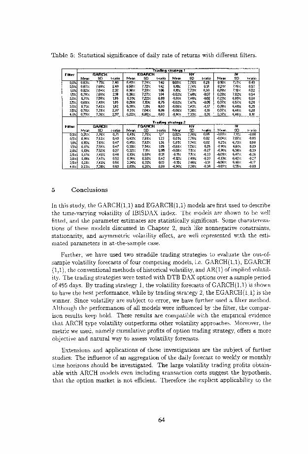
Table 5: Statistical significance of daily rate of returns with different filters.

5

Trading Rralcg, 1 Filtrr GARCH EGARCH HV IV

Mean SD r-rxia Mean SD t-ratio hlean SD t,xio Mean SD t-ratio 0.0% 0.83% 7.71% 2.40 0.4%! 7.71% 1.40 0.09% 7.76% 0.26 0.18% 7.17% 0.49 0.5% 0.87% 7.68'/. 2.49 0.50% 7.72% 1.42 0.W 7.74% 0.31 021% 7.15% 0.57 LO% 0.82% 7.8W 2.32 0.36X 7.33-L 1.08 0.w 7.732 0.30 0.20x 7.10% 0.52 1.5% 0.78% 7.60% 218 0.36% 7.27X 1.04 -0.02% 7.48% .0.07 020X 7.02% 0.54 2.0% 0.71% 7.55% 1.95 0.31% 7.22: 0.89 -0.01% 7.48% -0.02 0.23x 6.85% 0.60 2.5% 0.68% 7.49x 185 026X 7.15% 0.75 -0.02% 7.47% -0.05 0.07% 6.57% 0.20 3.0% 0.71% 7.42% L92 0.30% 7.w 0.83 -0.05% 7.43% -0.17 0.09% 6.48% 0.25 3.5% 0.78% 7.39% 2.07 0.31% 7.ow 0.86 -0.06X 7.38% -0.18 0.07% 6.46% 0.20 4.w 0.79% 7.36% 2.07 02% 6.80% 0.53 -0.14% 7.33% -0.39 0.07x 6.46% 0.18

Conclusions

Trading EGARCH

Medn SO t-ratio OAl% 7.75% 1.17 0.43% 7.69% 1.23 0.45% 7.621 1.26 0.39% 7.54x 1.09 0.32X 7.11% 0.95 im 6.68% 6.31 0.11% 6.59% 0.42 0.04X 6.33% 0.l3 0.02 6.264 0.08

rateg,Z HV

Mean SD t-ratio 0,02% 7.X% 0.05 0.01% 7.X% 0.02 0.01% 7.74x 0.02

-0.09% 7.56% -026 -0.03% 7.51% -0.27 -0.W 7.51% -0.33 -0.12% 7.49% -0.33 -0.w 7.46% -0.31 -0.14% 7.38% -0.38

.- Mean SD I-ratio -0.03% 7.11% -0.08 .0.04% 7.07% -0.09 -0.21% 6.73% -0.58 -0.14X 6.61% 0.39 -0.W 6.58% -0.39 -0.0% 6.47% Q.26 -0.10% 6;42% -0127 -0.06% 6.40'1 -0.17 -0.03% 8.35% -0.09

In this study, the GARCH(l,l) and EGARCH(l,l) models are first used to describe the time-varying volatility of IBISDAX index. The models are shown to be well fitted, and the parameter estimates are statistically significant. Some charatereza- tions of these models discussed in Chapter 2, such like nonnegative constraints, stationarity, and asymmetric volatility effect, are well represented with the estimated parameters in at-the-sample case.

Further, we have used two straddle trading strategies to evaluate the out-of- sample volatility forecasts of four competing models, i.e. GARCH( l,l), EGARCH (l,l), the conventional methods of historical volatility, and AR( 1) of implied volatility. The trading strategies were tested with DTB D-44X options over a sample period of 495 days. By trading strategy 1, the volatility forecasts of GARCH(l,l) is shown to have the best performance, while by trading strategy 2, the EGARCH(1,l) is the winner. Since volatility are subject to error, we have further used a filter method. Although the performances of all models were influenced by the filter, the comparison results keep hold. These results are compatible with the empirical evidence that ARCH type volatility outperforms other volatility approaches. Moreover, the metric we used, namely cumulative profits of option trading strategy, offers a more objective and natural way to assess volatility forecasts.

Extensions and applications of these investigations are the subject of further studies: The influence of an aggregation of the daily forecast to weekly or monthly time horizons should be investigated. The large volatility trading profits obtain- able with ARCH models even including transaction costs suggest the hypothesis, that the option market is not efficient. Therefore the explicit applicability to the

64

question of efficient portfolio insurance of volatile funds using options should be considered. This is left for future research.

65

References

[l] Akaike, H. (1973): “Information Theory and an Extension of the Maximum Likelihood Principle”, Second International Symposium on Information The- ory, B.N. Petrov and F. Csaki (eds.), Akademiai Kiado, Budapest, 267-281.

[2] Akaike, H. (1978): “T’ ime series analysis and control through parametric models”, Applied Time Series Analysis, D.F. Findley (ed.), Academic Press, New York, l-23.

[3] Berndt, E. K., Hall, B. H., Hall, R.E. and Hausman, J.A. (1974): .‘ Estimation Inference in Nonlinear Structural Models”, Annals of Economic and Social Measurement, 4, 653-665.

[4] Bollerslev, T. (1986): “Generalized Autoregressive Conditional Heteroskedas- ticity”, Journal of Econometrics, 31, 307-327.

[5] Box, G.E.P. and Jenkins, J.M. (1976): Time Series Analysis: Forecast- ing and Control, Hulden-Day, San Francisco.

[6] Engle, R.F. (1982): “Autoregressive Conditional Heteroskedasticity with Es- timates of the Variance of United Kingdom Inflation”, Econometrica, 50, 987-1008.

[7] Lu, Jian. (1998): “ARCH Volatility: characterizations, diffusions limits and an empirical application to DTB DAX option trading”, Diplomarbeit, Uni- versity of Mannheim.

[8] Natenberg, S. (1994): Option Volatilzty k Priczng: Advanced Tradzng Strate- gies and Technzques, Probus.

[9] Nelson, D.B. (1991): “Conditional Heteroskedasticity in Asset Returns: A New Approach”, Econometrzcal 59, 347-370.

[lo] Noh, J., Engle, R.F., and Kane, A. (1994): “Forecasting Volatility and Option Prices of the S&P 500 Index”, Journal of Deri,vatives. 1994, 17-30.

[ll] Wilkie, D. (1995): “More on a Stochastic Asset Model for Actuarial Use”, Britisch Actuarial Journal, Vol. 1, Part V, No 5, 777-964.

66

volatility forecasting and delta-neutral volatility

Documents