I POLICY RESEARCH WORKING PAPER 1226

Forecasting Volatility Methods for for casting tong-

in Commodity Markets run commodity price volatility

that combine time-series

modeling with market

expectations derived fromKenneth F. Kroner options prices outperform

Detvin P. Kneafsey forecast methods using only

Stijn Claessens market expectations or oniy

time series.

The World BankInternationai Economics Department

Debt and International Finance Division

November 1993

Pub

lic D

iscl

osur

e A

utho

rized

Pub

lic D

iscl

osur

e A

utho

rized

Pub

lic D

iscl

osur

e A

utho

rized

Pub

lic D

iscl

osur

e A

utho

rized

Pub

lic D

iscl

osur

e A

utho

rized

Pub

lic D

iscl

osur

e A

utho

rized

Pub

lic D

iscl

osur

e A

utho

rized

Pub

lic D

iscl

osur

e A

utho

rized

POLI(Y RESEARC-H WORKING PAPFR 1226

Summary findingsComnmodity prices have historically been amiong the CoMiModit at a cert ain dILt at a ti xed (exercise) price.most volatile of international prices. Measured Options prices depend on several vari-bles, ofne otvolatility (ttie standard deviation of price changes) has W hic i iI th eCxpected volatilitN up to the nuat i- ir date.not been below 15 percent and at times has been morc Given a spc.ific th oretical nodel, thc lmarket prics otthan 50 percent. Ofte the volatility of comimiiodity vptio(.1 CMhe [I e(1d to derive tht market s expc.;tionsprices has exceeded that of exclhanige rates and inttrest about price volatility and the price distribmrior.rates. Kroner, Krnafsev, anid C(lae'sens svstemalticalvl

The large price variations aire caused by disturbances analyze differe-rt iet hods' abilities to for Ccastin demand and supply. Stocklioldinig leads to some1c comimiOdity price volatiiity (for several ioniniodities).price smoothing, but wheni stocks ire low, prices CnI They collccted the daily prices of comimniodity optionsjurnp sharply. As a resLult, commnodity price series are anci other variables for seven commodities (cocoa,not stationary and in some periods they jump abruptly corni, cotton, gold, silver, sugar, and wheat). Theyto high levels or fall precipitously to low levels relative extracted the volatility forecasts iilplicit in optionsto their long-run average. 'Thus it is difficult to prices using icveral techniqUes. They compared severaldetermine long-term price trends and the uriderlying volatility forecasting methods, divided into threedistribution of prices, categories:

The volatility of commodity prices makes price (I) Forecasts usinig only expcctations derived fromforecasting difficult. Indeed, realized prices often options prices.deviate greatly from forecasted prices, which hals led to (2) ForCCasrs uSitng 0nIv timei-series miodeliig.the practice of giving forecasts probability ranges. But (3) Forecasts rhat cormilniie market expe';tations andassigning probability raniges reqtiii s forecasting future time-series mocdeling (a nue mthtocd devised for thisprice volatility, which, given uncertainties about true purpose),price distribution, is difficult. Ihtiv fir d that the volartili-y forecasts prodLce ih

Onie potentially useful source of intormiatio n for metho o d 3 ( tpertiorm the firsr two as vell as hth naiveforecasting volatility is thle volatility torecasts torecast hased on historical *olatilitv IThis result hioldsimbedded in the prices of optionis written o0n horh in and on t of simple for almost all conmmtoditiescomniodities traded in exchanges. Options give the consiid-red.holder thle right to buy (call) or sell (put) a certain

This paper- a product of the Debt and Internationial F inince l)Ivision, Ir rerna t ional con omics Department -is partof a larger effort in the departmenit to study the short- and long- run behavior of primary conimiodity prices and theimplications for developing countries of movemernts in these prices. The study was funded hy the Bank's ResearchSupport Budget under the research rroject 'Measurernent of Commodity Price Vo!atility" (RPO 676-73). Copies ofthis paper are available free fro<m the World Bank, 181 8 H Street NW, Washlington, D)C 20433. Please contact FatenHatab, room H8-099, extension 35835 (22 pages). November 1993.

I 7'he Poliy iResearch Working Paper Series disse ;inatcs t!u nd:ings of isork in /'r,jgr(5s t; 'ii. ,u'a;e tfc exfl'hanve d O,WS .,',Ut

development issues. An objective of the series is toget thte findin's ourt quicklv. c en in the presentatri <arc , lss thn tuil; ),Iise/l. Ii'papers carrv the names of the authors and ihould bcl used and (u,d zco'rditnel. /lI'iendins. rnt,'r( letv,uns, .iand ,rn, lsiois are, te|authors' own and should not be attributed to) the 'Torld liank, its 1 .xCcutii 'lri 'if t, r'. lr a " 54

Produticed bs the Policy Rcsearchi Disscmiriation Centel

Forecasting Volatility in Commodity Markets

KENNETH F. KRONEERDEPARTMENT OF ECONOMICS

UNIVERSITY OF ARIZONATUCSON, AZ 85721

(602) 621-6230

I(EVN P. KNEAFSEYDEPARTMENT OF FINANCEUNIVERSITY OF ARIZONA

TUCSON, AZ 85721(602) 621-1716

STIJN CLAESSENSDEBT AND INTERNATIONAL FINANCE

WORLD BANK1818 H ST, NW

WASHINGTON, D.C. 20433(202) 473-7212

Summary

Commodity prices have historically been one of the most volatile of international prices.Measured volatility (the standard deviation of price changes) has not been below 15% and attimes has been more than 50%. During many periods the volatility of commodity prices hasexceeded the volatility in exchange rates and interest rates. The cause of the large pricevariations are disturbances in demand or supply. Stockholding leads to some price smoothingbut when stocks are low, prices can jump very sharply. As a result, commodity price serieshave two important features. First, they display non-stationarity. Second, there are periodswhen prices jump abruptly to very high levels (or fall to very low levels) re!ative to their longrun average. These two features make it very difficult to determine the long-term price trendand the nature of the underlying distribution of prices.

The high levels of commodity price volatility make price forecasting extremely difficultand, indeed, large ex-pgs deviations of realized prices from forecasted prices are common.This has motivated the practice of providing probability ranges around the forecast. This, inturn, requires forecasts of future price volatility which, given the uncertainty about the natureof the true price distribution, has also proven difficult. One potentially useful source is thevolatility torecasts imbedded Ln prices of options written on commodity prices traded onexchanges. Options give the holder the right to buy (call) or sell (put) a certain commodity ata certain date at a fixed (exercise) price. Option prices depend on a number of variables, oneof which is the expected volatility over the horizon to the maturity date. Thus, given a specifictheoretical model, market prices of options can be used to derive the market's expectation ofprice volatility and the price distribution.

This paper provides a systematic analysis--covering several commodities--of the abilityof different methods of forecasting commodity price volatility. Daily prices of commodityoptions and other variables were collected for seven commodities (cocoa, corn, cotton, gold,silver, sugar and wheat). The volatility forecasts implicit in the option prices were thenextracted using several techniques. The paper compares several different forecasts of commodityprice volatility, divided into three categories: (1) forecasts using only expectations derived fromoptions prices; (2) forecasts using only time series modelling; and (3) forecasts which combinemarket expectations and time series modelling. Methods (1) and (2) have been used extensivelyin the literature, while use of method (3) for this purpose is new. The paper finds thatcombining market expectations and time series modelling (method (3)) gives volatility forecastswhich outperform both market expectations forecasts and time series forecasts as well as thenaive forecast based on historical volatility. This iesult hold both in and out of sample forvirtually all commodities considered. These results hold promise for deriving probabilitydistributions for commodity price forecasts which will perform considerably better than methodsnow being used.

I. Introduction.

Commodity prices have historically been one of the most volatile of international asset prices.

Over the period 1972-1990, for example, the volatility of non-oil commodity prices in nominal terms,

as measured by the annualized standard deviation of percentage changes during the previous 24

months, was not below 15% and peaked at more than 50% in 1975. It is not surprising, then, that

efforts to forecast commodity prices have been large'y unsuccessful. In fact, it can be expected

that ex-post forecast errors will continue to display a large distribution around zero, whether the

forecasts are made using futures prices or specialists' assessments. For this reason, it is important

to construct a measure of confidence in the price forecast. The traditional way to express confidence

in a forecast is to bound t by a confidence interval, that is, to give an interval forecast and an

associated probability. This is easily done in a world where volatility is const. at, but if volatility

is itself changing, then . forecast of volatility must be derived before an interval forecast can be

constructed. Volatility forecasts ar3 also crucial in the pricing of options contracts because all else

equal, a higher forecasted volatility should result in higher options prices. So an investor with a

better forecast of volatility than the market's should be able to exploit the fLrecast to make exces-

returns.

The purpose of this paper is to develop methods of forecasting commodity price volatility over

long time horizons, here taken as 225 days. Several methods of forecasting volatility over -hHrt

horizons already exist in the literature, but many of these methods do not carry over to i .g-

horizon forecasts. For example, implied standard deviation forecasts derived from options prices

as in Latane and Rendelman (1976), Beckers (1981), Wei and Frankel (1991), and many others,

may be appropriawe for short-term forecasts, but are unreliable for long-term forecasts because

trading is very thin in options that are far from their expiration dates. Also, traditional time series

methods, like ARMA models on moving standard deviations as in Cao and Tsay (1991), or ARMA

models on bid-ask spreads or daily price ranges, as in Taylor (1987), are not likely to give useful

forecasts because a 225-day forecast will generally be simply the unconditional mean of the series.

To illustrate, the 225-day forecast from the ARMA(1,1) model

Ye = w + oyt-, + oEt-l + ft

is

Y+s= w (E 0 @2 ) + 92 25 y, + o2 24 of,

We would like to thank seminar participants at the World Bank for their useful suggestions. All errors are ours alone.

1

which is approximately w/l1 - 0) if 1J1 < 1. Wle develop a forecasting model which combinesinvestors' forecasts with time series forecasts, and produces forecasts of long-term volatility whichare more accurate than the short-term forecasting methods. This result holds both in-sampleand out-of-sample for almost all of the commodities we consider, suggesting that our proposedforecasting model can be an effective tool for constructing interval forecasts and for the pricing oflong-term options. The paper is organized as follows: Section II discusses some short-term volatilityforecasting methods and Section III presents our new forecasting framework. Section IV discussesthe data, Section V presents the results, and Sectior. VI concludes.

II. Exist'ng Forecasts.

I.1. Implied Standard Deviations. One popular method of forecasting volatility uses optionprices to measure investors' expectations of future volatility. An option is a contract which permaits,but does not require, the holder to buy (sell) the underlying asset at a preAetermined price. C:early,the more volatile the price of the underlying asset, the more likely it is that the option will havevalue, consequently the higher the option's price. If the option m .rket is efficient, then investors'expectations of future volatility as embodied in option prices should be the best volatility forecastavailable. Mlore specifically, option prices are functions of four observable variables (the price ofthe underlying asset, the exercise price of the option, the time to maturity of the option, aDdthe risk-free rate of interest) and one unobservable variable (the expected volatility of returns onthe underlying asset over the life of the option). Since the option price is itself observable, andsince the option price is a monotonically increasing function of expected volatility, one can use anoption pricing model to back out the market's expectation of volatility over the remaining life ofthe option (Latane and Rendleman, 1976). This forecast of volatility is often called the impliedstandard deviation, or ISD. We refer to it as a "market-based" forecast because it is based entirelyon the expectations of participants in the options market (given a particular option pricing model).

To compute the ISD we require an option pricing formula for commodity futures options.Most options on commodities are American options, m-ining that they can be exercised either at,ny date on or before maturity or at any time within a Epecific period (e.g., one month) beforematurity1 . This early exercise feature of commodity options means that they should sell at a

1 Early exercise is important when dealing with options on futures contracts. ignoring ;torage costs and convew., ,, yields, the futures price is F(T) = SoerT, so the futures price declines to the spot price as expiration nears i , .makes the behavior of futures prices similar to that of a stock price that pays out continuous dividends. These 'inii. ,dividends" can only be reaped if the option holder exercises the option.

2

premium relative to European options, which allow the option holder to exercise the option only on

the maturity date of the option. This in turn means that the use of the standard European option

pricing formula of Black (1976) will result in ISD's which are overstated. The positive bias in the

ISD occurs because the European formul3 assumes that the higher option price is due to nigher

volatility (and therefore a higher estimated ISD is obtained), when il reality the higher price simply

reflects the early exercise premium2. Unfortunately, no closed-form solution exists for American

options, though several approximation methods exist. We adopt the method of Barone-Adesi and

Whaley (1987), who provide an efficient approximation for pricing American options on commodity

futures.

Suppose that the underlying futures price follows the stochastic differential equation

(1) dF/F = Cdt + odz,

where F is the commodity futures price, C is the iastantaneous expected relative price change of the

commodity, a is the instantaneous standard deviation, t is time and z is a Wiener process. Then

if the- interest rate r is constant and no arbitrage opportunities exist, Black (1976) shows that the

price of a commodity futures option, C, must follow the partial differential equation

(2) 1a2F2CFF- rC + Ct 0 O

where subscripts represent partial derivatives of the variable with respect to the subscript. For a

European option with no early exercise privilege, the boundary condition requires that the maturity

value of the option be equal to max{O, FT - X}, where FT is the futures price at maturity and X

is the exercise price. This boundary condition is applied to (2) to get Black's European commoulty

futures option pricing formula

(3) c(Ft, T, r, X, a) = e-rT[FtN(d;) - XN(d 2 )],

where T is timue to maturity, N(.) is the cumulative normal distribution, and

di = [ln(Ft/X) + 2 Ta2]/o.Va

d2 = dI - aV.

2 To de..o.rstrate the potential magnitude of the bias, consider the May/1985 soybean futures option selling on Noverii .-r

2, 1984 with an exercise price of S600. The futures price war 8664.75, the spot price was 8627.50, the call price ' i%

876.00, ani the annualized interest rate was 9.737%. Using Black's (1976) formula for pricing European futures opLon.ie ISD is 0.2272, while using the Barone-Adesi and Whaley American option pricing approximation (which will t.

cussed 3hortly), the ISD is 0.2174. The overstatement using the European formula is thu: about 5%.

3

However, when early exercise is possible, the American option boundary conditions must be used,

and a closed form solution no longer exists. Barone-Adesi and Whaley (1987) propose an approxi-

mate solution to this problem. Without going into the details of their derivation, define

A2 = (FO/q 2 ){1 - e-rTN(d;)}

d; = [ln(F-/X) + 2a aTJ/Ia7

q2 = [1 + Vl + 8r/(oTK)]/2

K = 1 - '

where F' is the futures price that satisfies

F- - X = c(F, T, r, X, o) + {1 - e-,TN(d;)}F'1q2

and c(.) is Black's theoretical call price in equation (3) above. Then the approximate formula for

the price of an American commodity futures call option at time t, C(Ft, T,r,X, o), is

r c(F, T, r, X, cr) + A2(F1 /F*)q2 if Ft < F-(4) CF,T,r,X,a) = F-X if=F F.

Three important observations merit mention. First, while this formula is mathematically com-

plicated, it is easily programmed. Second, Barone-Adesi and Whaley (1987) show that this ap-

proximation becomes exact as the time to expiration gets large. In this paper we are focusirl on

long-horizon forecasts, so the approximation error should be quite small. And third, notice that

thei are only six variables in this formula - C, X, F, r, T and o. The first five are observable

and therefore can be used to solve for a. This o, the ISD, is the measure of volatility implied by the

option price, that is, the market's expectation of volatility over the remaining life of the contract.

In this paper we will evaluate a set of forecasts based on ISD's. But for any given day in

our data set and lor any given option maturity, there are several different options traded, one for

each exercise price. For example, on Nov 2, 1988, there were 20 wheat contracts which expired

in March 1989, each with a different strike price. Therefore, we can extract 20 different ISD's,

or twenty different forecasts of volatiiity between Nov/88 and Mar/893 , one from each contract.

We used three different methods to collapse these multiple ISD forecasts into a single volatility

forecast. The first takes the ISD from the contact for which the price of the option is most sensiti i

3 All 20 of these forecasts do not return the same ISD. The fact that they do not is an indication of one or morp ,'the following: option market inefficiencies; the impact of price discreteness in an option pricing model that assljrIIrcontinuous prices; and/or misspecification in the option pricing model.

4

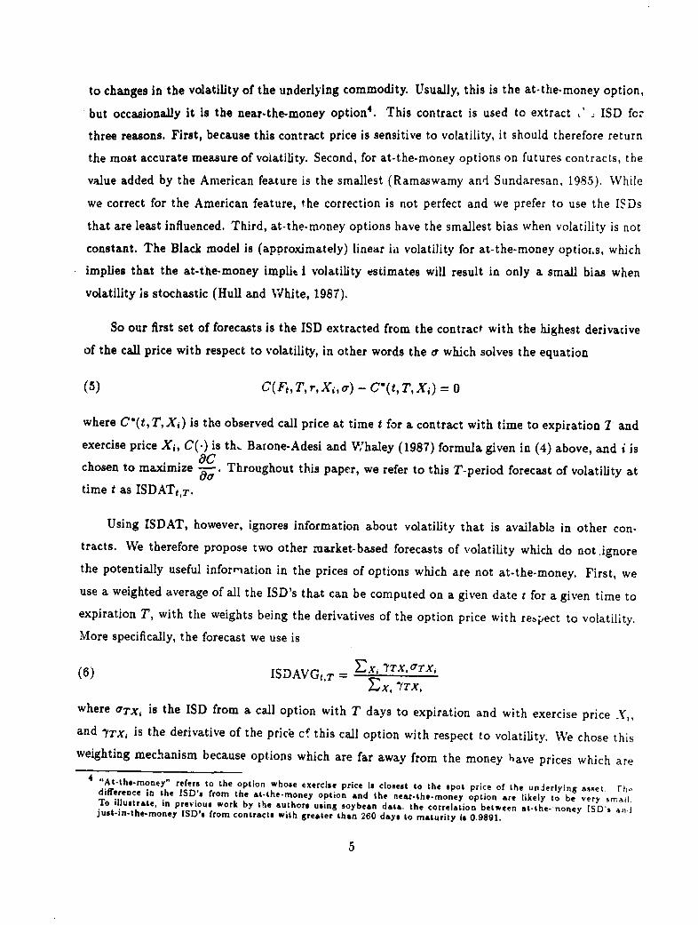
to changes in the volatility of the underlying commodity. Usually, this is the at-the-money option,but occasionally it is the near-the-money option4. This contract is used to extract .' ISD fc.three reasons. First, because this contract price is sensitive to volatility, it should therefore returnthe most accurate measure of volatility. Second, for at-the-money options on futures contracts, thevalue added by the American feature is the smallest (Ramaswamy and Sundaresan, 1985). Whilewe correct for the American feature, the correction is not perfect and we prefer to use the ISDsthat are least influenced. Third, at-the-money options have the smallest bias when volatility is notconstant. The Black model is (approximately) linear hi volatility for at-the-money optioL.s, whichimplies that the at-the-money implit I volatility estimates will result in only a small bias whenvolatility is stochastic (Hull and White, 1987).

So our first set of forecasts is the ISD extracted from the contract with the highest derivaciveof the call price with respect to volatility, in other words the a which solves the equation

(5) C(Ft,T,r, Xi,o) - C(t,T,Xi) = 0

where C'(t,T,X,) is the observed call price at time t for a contract with time to expiration 7 andexercise price Xi, C(-) is th, Barone-Adesi and W'haley (1987) formula given in (4) above, and i ischosen to maximize T. . Throughout this paper, we refer to this T-period forecast of volatility attime t as ISDATteT.

Using ISDAT, however, ignores information about volatility that is available in other con-tracts. We therefore propose two other market-based forecasts of volatility which do not ignorethe potentially useful inforrnation in the prices of options which are not at-the-money. First, weuse a weighted average of all the ISD's that can be computed on a given date t for a given time toexpiration T, with the weights being the derivatives of the option price with rebpect to volatility.More specifically, the forecast we use is

(6) ISDAVGtT = Ex, YTX.OTX

where °TXj is the ISD from a call option with T days to expiration and with exercise price Y,,and 7TX, is the derivative of the price cf this call option with respect to volatility. We chose thisweighting mechanism because options which are far away from the money have prices which are

4 "At-the-money" refers to the option whose exercise price is closest to the spot price of the underlying asset, rhidifference in the ISD's from the at-the-money option and the near-the-money option are likely to be very smailTo illustrate, in previous work by the authors using soybean data. the correlation between at-the- noney ISD's an,jjust-in-the-money ISD's from contracts with greater than 260 days to maturity is 0.9891.

5

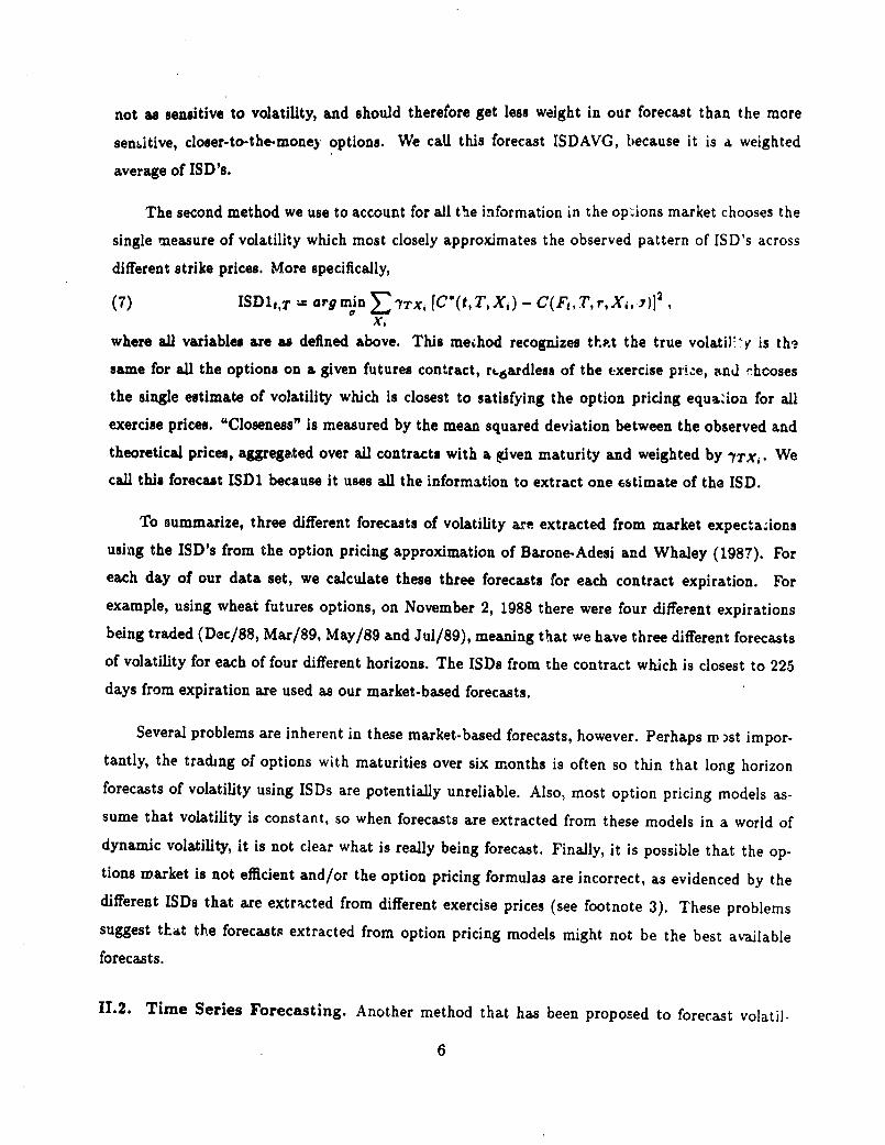
not as sensitive to volatility, and should therefore get less weight in our forecast than the moresensitive, closer-to-the-money options. We calU this forecast ISDAVG, because it is a weighted

average of ISD's.

The second method we use to account for all the information in the opsions market chooses thesingle mneasure of volatility which most closely approximates the observed pattern of ISD's across

different strike prices. More specifically,

(7) ISD1,T -= argmin ETXS [C*(t,T,X,) - C(Ft,T,r,Xi,7)]2Xi

where all variables are as defined above. This mechod recognizes thma the true volatil'y is thesame for all the options on a given futures contract, rc6ardless of the exercise pri.e, and 'hcoses

the single estimate of volatility which is closest to satisfying the option pricing equa'ion for all

exercise prices. "Closeness" is measured by the mean squared deviation between the observed and

theoretical prices, aggregated over all contracts with a given maturity and weighted by -tTx,. We

call this forecast ISD1 because it uses all the information to extract one estimate of the ISD.

To summarize, three different forecasts of volatility are extracted from market expectaJions

using the ISD's from the option pricing approximation of Barone-Adesi and Whaley (1987). Foreach day of our data set, we calculate these three forecasts for each contract expiration. Forexample, using wheat futures options, on November 2, 1988 there were four different expirations

being traded (Dec/88, Mar/89, May/89 and Jul/89), meaning that we have three different forecastsof volatility for each of four different horizons. The ISDs from the contract which is closest to 225days from expiration are used as our market-based forecasts.

Several problems are inherent in these market-based forecasts, however. Perhaps rn )st impor-tantly, the trading of options with maturities over six months is often so thin that long horizon

forecasts of volatility using ISDs are potentially unreliable. Also, most option pricing models as-sume that volatility is constant, so when forecasts are extracted from these models in a world ofdynamic volatility, it is not clear what is really being forecast. Finally, it is possible that the op-tions market is not efficient and/or the option pricing formulas are incorrect, as evidenced by thedifferent ISDs that are extracted from different exercise prices (see footnote 3). I'hese problemssuggest thAt the forecasts extracted from option pricing models might not be the best available

forecasts.

II.2. Time Series Forecasting. Another method that has been proposed to forecast volatil.

6

ity involves time series modelling of the variances (see, for example, Engle and Bollerslev, 1986).

Many assets are characterized by time varying variance, and consequently require dynamic models

of volatility. One set of models which has become poFular in finance is the Autoregressive Condi-

tional Heteroskedasticity (ARCH) and Generalized ARCH (GARCH) models of Engle (1982) and

Bollerslev (1986), in which variances are modeled as an ARMA process. The popularity of GARCH

models stems from their ability to capti!re volatility clustering, a feature common 'o financial time

series. See Bolleislev, Chiou and Kroner ( 992) for a survey of GARCH applications in 9nancial

modelling.

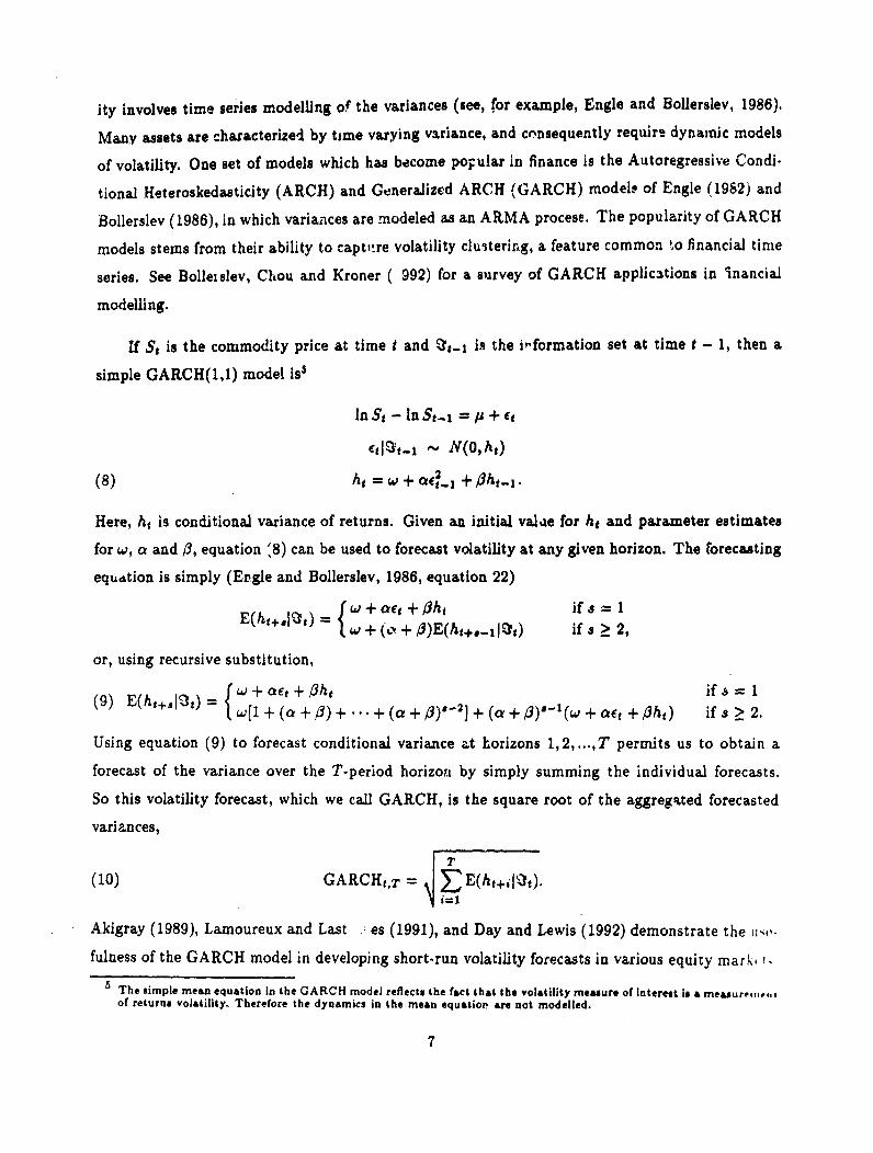
If St is the commodity price at time t and %-, is the iv'formation set at time t - 1, then a

simple GARCH(l,l) model iss

InSg - In St. = / + et

e.j!a_j - lN(O,h,)

(8) hi = w + aret_l +,Oht-1.

Here, ht is conditional variance of returns. Given an initial valu.e for ht and parameter estimates

for w, a and 13, equation '8) can be used to forecast volatility at any given horizon. The forecasting

equation is simply (Engle and Bollerslev, 1986, equation 22)

E(ht+.Ijt) f w+ act +i3h if a= I=w + (c, + O)E(ht+.-..1I) if a > 2,

or, using recursive substitution,

{ E % + act + 3ht if s = 1

(9) E(ht+aI~3t) w[1+(a + )) + . + (a + 3) -2] + (a + + act+ i3ht) ifs >_ 2.

Using equation (9) to forecast conditional variance at horizons 1,2,...,T permits us to obtain a

forecast of the variance over the T-period horizon by simply summing the individual forecasts.

So this volatility forecast, which we call GARCH, is the square root of the aggregated forecasted

variances,

(10) GARCHt,T = EE(ht+1j)

Akigray (1989), Lamoureux and Last es (1991), and Day and Lewis (1992) demonstrate the ti,o-

fulness of the GARCH model in developing short-run volatility forecasts in various equity mark--,

The simple mean equation in the GARCH model reflects the fact that the volatility measure of interest is a measure,..,.of returns volatility. Therefore the dynamics in the mean equatior are not modelled.

7

A second time series-based forecast o, volatility, which is bafied only on historical returns, is

included in our ., mparisons as a simple benchmark that at a minimum more complex models must

beat. This forecast, which we call HISTt,T (for historical), is simply the sample standard deviation

of returns over the previous 7 weeks. This forecast is included because Bartunek and Mfustafa(1991) find that for the stocks they used, it outpeiformed botlh ISD-based forecasts and GARCH-

based forecasts for long horizons (80 and 120 days). However, this result seerns to contradict much

of tile extant literature.

To summarize, in addition to the three ISD-based forecasts, we also have two time series-based

forecasts of volatility. The first pure time series method uses a GARCH model to forecast volatility

over the remaining life of the contract and the second time series methc -, HIST, uses the sample

variance of returns over the previous seven weeks as a forecast of future volatility. But pure time

series models, by definition, ignore the market's expecta'ions of the future volatility and rely solely

on the information contained in the past data. Conscquently, we propose a third class of volatility

forecasts which incorporates both time series analysis and market expectations of volatility.

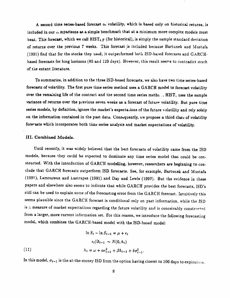
III. Combined Models.

Until recently, it was widely believed that the beat forecasts of volatility came from the ISD

models, because they cotild be expected to dominate any time series model that could be con-structed. With the introduction of GARCH modelling, however, researchers are beginning to con-clude that GARCH forecasts outperform ISD forecasts. See, for example, Bartunek and Mustafa

(1991), Lamoureux and Lastrapes (1991) and Day and Lewis (1992). But the evidence in thesepapers and elsewhere also seems to indicate that while GARCH provides the best forecasts, ISD's

still can be used to explain some of the forecasting error from the GARCH forecast. Intuitively thisseems plausible since the GARCH forecast is conditional only on past information, while the ISDis v measure of market expectations regarding the future volatility and is conceivably constrli rtcrd

from a larger, more current information set. For this reason, we introduce the following forecastingmodel, which combines the GARCH-based model with the ISD-based model:

InSt - IlnSt-, = / + et

f tPlt-i N(0, ht )

(11) ht = w + ae + ihi- 1 + bo2.

In this model, at-, is the at-the-money ISD from the option having closest to 100 days to expiratirI,

8

extracted from equation (5). If the 100-day ISD implies that early exercise is optimal, then we used

the 100-day ISD from the previous day.6 Models like this have been estimated before (see, for

example, Day and Lewis, 1992), but only in the context of tests for market efficiency. They have

not been used in forecasting exercises. The idea behind the market efficiency test is that if the

options market is efficient then the ISD backed out from a properly specified options pricing model

should capture all of the volatility of the spot prices that can be predicted based on the current

information set. nhe implication is that all of the coefficients in the variance equation of model

(11, should be zero except for the coefficient on the ISD term. If either a or p3 remains significant

upon inclusion of the ISD term, then there is information in the past time series of volatility which

is not incorporated in the market's expectations of future volatility, but is relevant in predicting

future volatility. This implies that the options are mispriced and past volatility data can be used

to take advantage of the mispricing.

Forecasts from this model are made with the following equation:

(12) E(ht+dIZ.) = 1 ifs= 16 = + 6o0 + (a + I)E(ht+._ijjt) ifs 2 2,

Again, we forecast ht+. for each period between now and our forecast horizon, and the square root

of the sum of these forecasts is our forecast of volatility:

T(13) COMBt,T = E E(ht+ °')'

where E(ht+il!t) is compu.ed from equation (12). We call this forecast COMBt,T because it

combines the ISD and GARCH forecasts. This gives us six forecasts of volatility: 3 ISD forecasts,

2 time series forecasts, and a combination ISD and GARCH forecast.

IV. Data.

The forecasting methods presented above are evaluated using daily data for cocoa, corn, cotton,

gold, silver, sugar and wheat. The time span covered for each commodity varies slightly, depending

on data availability, but usually extends from about January 1987 - November 1990. The ISD-based

forecasts require data on futures prices, interest rates and options prices. The futures data is daily

closing prices, obtained from Knight-Ridder Financial Services. The interest rates we use are 1 l

6 We found that the horizon of the ISDs did not matter in equation (11). We therefore used 100-day ISDs instea l ,.225-day ISDs because they are much more heavily traded and are much more commonly Vnalyzed in the literaturp

9

treasury biU rates from the bill which expires closest to the time the option expires, as provided by

Data Resources, Inc. The options price data for corn and wheat is daily closing prices, obtained from

the Chicago Board of Trade, while the rest of the options data is daily closing prices, obtained from

Data Resources, Inc. Information regarding the features of various options and futures contracts

(such as the last trading day, contract months, etc.) is taken from the descriptions published by the

different commodity exchanges. Table 1 provides a brief overview of the options data by commodity

and serves to illustrate the magnitude of the data sets and the breadth of contracts traded per day.

TABLE 1

The GARCHt,T and HISTt,T forecasts require spot price data, which was obtained from Data

Resources, Inc. In order to evaluate the forecasts, a measure of the 'true" 225-day volatility is

needed. One measure used in the literature and the one which we use here, is the realized standard

deviation of returns over the forecast horizon. This is computed by calculating the square root of

the average daily squared return over the forecast horizon. This is called ACTUAL to represent

the actual volatility of returns over the period of interest. Clearly, comparing the various long-run

forecasts to ACTUAL requires spot data which extends 225 days beyond the last option data, so

the time span covered by our spot data is from about January 1987 - July 1SJl.

V. Estimation and Results.

The three ISD-based 225-day volatility forecasts are computed from equations (5), (6) and (7)

above. In order to construct the GARCH forecast and the COMB forecast, we need to estimate

the GARCH model (equation 8) and the COMB model (equation 11). The relevant maximum

likelihood estimates are presented in Table 2, with asymptotic t-statistics in parentheses7 . The

Q2 statistic, which tests for remaining serial correlation in the standardized squared residuals and

is distributed X22 under the null of no remaining serial co.:elation, indicates that the estimated

models adequately capture the dynamics in the second moments. One result of interest is that for

many of the commodities (cotton and wheat are the exceptions), the variance equation coefficients

sum to approximately one (i.e. a + d t 1). This means that shccks to the variance are persistent,

i.e., shocks remain important determinants of the variance forecasts long after the shocks occur.

This is easily seen by setting a +3 = 1 in the second line of the GARCH forecasting equation (9).

The observation period used in estimating these models excluded the final eight weeks of our sample (40 observations)in order to facilitate out.of-sample forecasting later in this paper.

10

giving

E(hg+,I%) = w(9 - 1) + ht+,.

In this case the optimal variance forecast is simply the forecast of tomorrow's variance, adjusted

for a drift component. This is important for our application because it implies that the long-term

forecast from the GARCH models will not revert to the unconditional variance, as is common in

long-run forecasts from ARMA models. Another result of interest is that the ISD in the combined

model is highly significant for all commodities examined, suggesting that market expectations can

help to predict variances. Also, the GARCH parameters (a and /3) tend to drop in significance

meaning that the ISD's capture much of the same information that GARCH does. This drop is most

noticable in 3. But the GARCH parameters tend to remain significant, suggesting a violation of

options market efficiency. In other words, the ISD's contain information about future volatility that

is not captured by the GARCH model, and the time series of volatility contains information about

future volatility that is not incorporated in the option price. This suggests that the COMB model,

which puts these two kinds of information into the same model, has potential to be a successful

forecasting model.

TABLE 2

For each commodity, the six different forecasts and the actual variance over a 225-day forecast

horizon are summarized in Table 3. Each block of the table presents summary statistics (average,

minimum, maximum and number of observations) for the actual and forecasted variance for each of

the different commodities studied8 . Also, to illustrate the relationships among the various forecasts,

Table 4 presents the correlation matrix for the corn forecasts. One observation from Table 3 is that

the ISD-based forecasts tend to overstate true volatility (except for cocoa and wheat). There are

several explanations for this, two of which are stochastic interest rates and stochastic volatility. For

example, if the interest rate is stochastic then the ISD wiU capture both asset price volatility and

interest rate volatility, so the ISD will be overstated. However, Ramaswamy and Sunderesan (1985)

show that using the actual term structure at each point in time (as we do) eliminates much of the

mispricing due to stochastic interest rates. Another observation is that the HIST forecast seems

to be very accurate, on average. This is surprising, given that it was constructed as the sample

8 In this table and the two which follow, the samples from which the statistics are computed do not include the final eightweeks of data, which were withheld for out-of-sample comparisons. This explains part of the difference between thenumber of observations listed in Table 3 and the number of days listed In Table 1. The remaining difference is causedby withholding the first 34 observations in order to enable computation of the HIST forec"ts. Also, the ISD basedforecasts have different numbers of observations because observations were dropped if the extracted ISD implied thatearly exercise wa optimal.

11

standard deviation over moving 7-week windows, and the actual volatility is the sample standarddeviation over the subsequent 225-day window. However, as we will see below, having an averageforecast error close to zero does not make it a good forecast. The second most accurate forecasts, onaverage, are the COMB forecasts, suggesting that combining market ex-ectations with time seriesmethodology might improve forecasting abil;.y. Another observation is that for some commodities(cotton, gold and perhaps wheat), the range of the GARCH forecasts is small, suggesting that theGARCH forecasts are almost constant. This is to be expected for long-horizon forecasts if a + B ismuch less than one (see equation 9), as is the case for cotton and wheat. Finally, we see from Table4 that the correlations among the three ISD forecasts are very high, and all correlations with HISTare low. We should therefore not be surprised if the ISD forecasts all perform similarly, while theHIST forecasts perform badly.

TABLES 3 AND 4

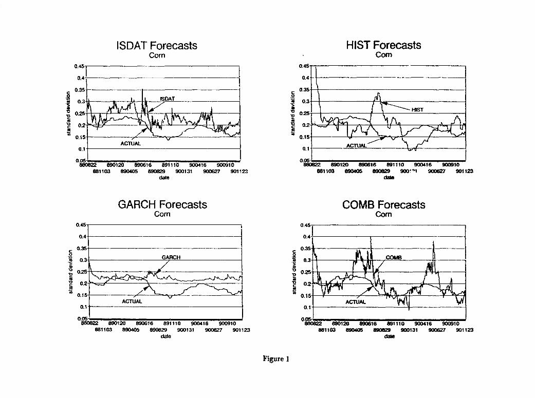
Many of these observations are evident in Figure 1, which presents the 225-day ISDAT, HIST,GARCH and COMB forecasts for corn along with the actual 225-day volatility.9 For example,it is clear that ISDAT tends to overstate volatility and that the GARCH forecasts are relativelystable. The HIST forecasts seem to have little relationship to the actual variance beinv' forecast,even though on average they might be close to the actual variance. The COMB forecasts seem totrack the true volatility quite well, though the swings in the COMB forecast are much bigger thanthe swings in the realized volatility.

FIGURE 1

We use mean squared forecast errors (MSFEs) to formally evaluate each of the forecasts. Othermetrics, like mean absolute forecast errors, gave virtually identical conclusions. Table 5 shows themean squared forecast errors for each of the forecasting models for each commodity. It is clear fromthe table that, with the exception of silver, the GARCH and COMB models dominate all of theISD forecasts and the historical volatility f-recasts. GARCH in particular forecasts well, having thesmallest MSFE for 4 of the 7 commodities and performing second best in two other cases. COMBhas the smallest MSFE for two of the commodities, and has the second smallest MSFF for threeothers. Also, as anticipated from Table 4, the ISD forecasts all perform similarly, and the HIS'rforecasts tend to perform the worst.

TABLE 5

9 W do not present graphs of ISDAVG and ISDI because they are very similar to the ISDAT graph.

12

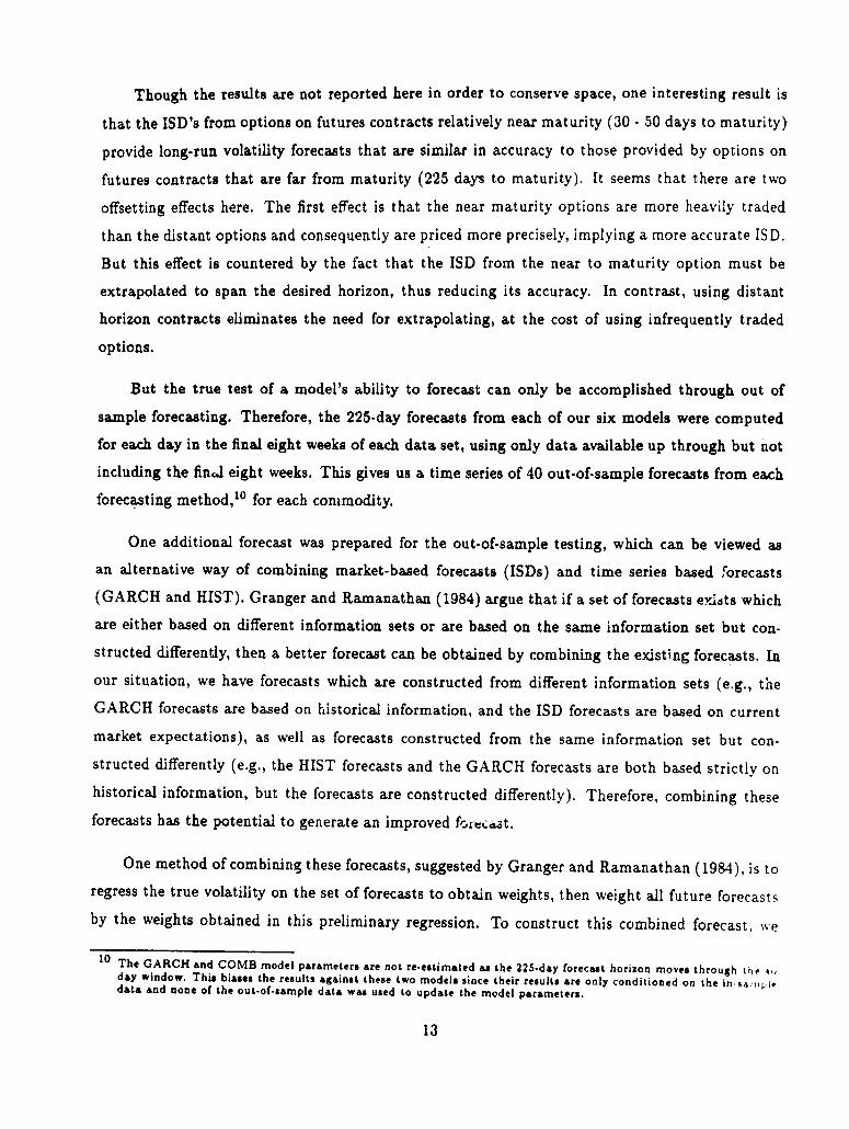
Though the results are not reported here in order to conserve space, one interesting result is

that the ISD's from options on futures contracts relatively near maturity (30 - 50 days to maturity)

provide long-run volatility forecasts that are similar in accuracy to those provided by options on

futures contracts that are far from maturity (225 days to maturity). It seems that there are two

offsetting effects here. The first effect is that the near maturity options are more heavily traded

than the distant options and consequently are priced more precisely, implying a more accurate ISD.

But this effect is countered by the fact that the ISD from the near to maturity option must be

extrapolated to span the desired horizon, thus reducing its accuracy. In contrast, using distant

horizon contracts eliminates the need for extrapolating, at the cost of using infrequently traded

options.

But the true test of a model's ability to forecast can only be accomplished through out of

sample forecasting. Therefore, the 225-day forecasts from each of our six models were computed

for each day in the final eight weeks of each data set, using only data available up through but not

including the fin.l eight weeks. This gives us a time series of 40 out-of-sample forecasts from each

forecasting method,1 0 for each commodity.

One additional forecast was prepared for the out-of-sample testing, which can be viewed as

an alternative way of combining market-based forecasts (ISDs) and time series based forecasts

(GARCH and HIST). Granger and Ramanathan (1984) argue that if a set of forecasts exists which

are either based on different information sets or are based on the same information set but con-

structed differently, then a better forecast can be obtained by combining the existing forecasts. In

our situation, we have forecasts which are constructed from different information sets (e.g., the

GARCH forecasts are based on historical information, and the ISD forecasts are based on current

market expectations), as well as forecasts constructed from the same information set but con-

structed differently (e.g., the HIST forecasts and the GARCH forecasts are both based strictly on

historical information, but the forecasts are constructed differently). Therefore, combining these

forecasts has the potential to generate an improved foft.ast.

One method of combining these forecasts, suggested by Granger and Ramanathan (1984), is to

regress the true volatility on the set of forecasts to obtain weights, then weight all future forecasts

by the weights obtained in this preliminary regression. To construct this combined forecast, we

10 The GARCH and COMB model parameters are not re-estimated as the 225-day forecast horizon moves through the 4,dday window. This biases the results against these two models since their results are only conditioned on the in-sampi,data and none of the out-of-sample data was used to update the model parameters.

13

withheld 200 observations from the end of our data sets1l and reestimated all the models. We then

ran the regression

(13) ACTUALt,2 2s = -lo + zylISDATt,22s + y2HISTt,2 2s + 73GARCHt,225 + 74 COMBt, 22S

to obtain the weights on the forecasts. We did not include ISDAVG and ISD1 in the regressionbecause they are highly collinear with ISDAT (see Table 4), and would therefore add little to

forecasting power. Table 6 presents the parameter estimates from (13) for each commodity. Notice

that for four of the seven commodities, the COMB forecast gets the highest (positive) weight,

suggesting that the GR forecasts are based more heavily on the COMB forecasts than the mark,.

based ISD forecasts. The negative weights which sometimes appear on the GARCH forecasts can

be attributed to multicollinearity with the constant. They all become positive when the constant

term is omitted from the regression12 . This linear combination of forecasts is guaranteed to provide

superior within-sample forecasts than any of the individual forecasts because it is chosen to rainimize

within-sample mean squared fo: 3cast error. This suggests, but does not guarantee, that it will

perform better out-of-sample as well.

TABLE 6

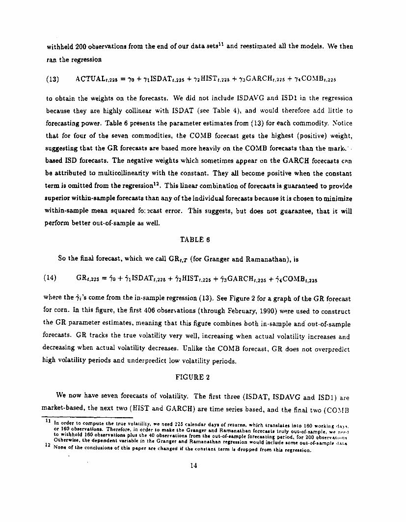
So the final forecast, which we caU GRt,T (for Granger and Ramanathan), is

(14) GRt,225 = lo + jiISDATt,225 + 5'2HISTt, 225 + l 3GARCHt,225 + j 4COMBt,225

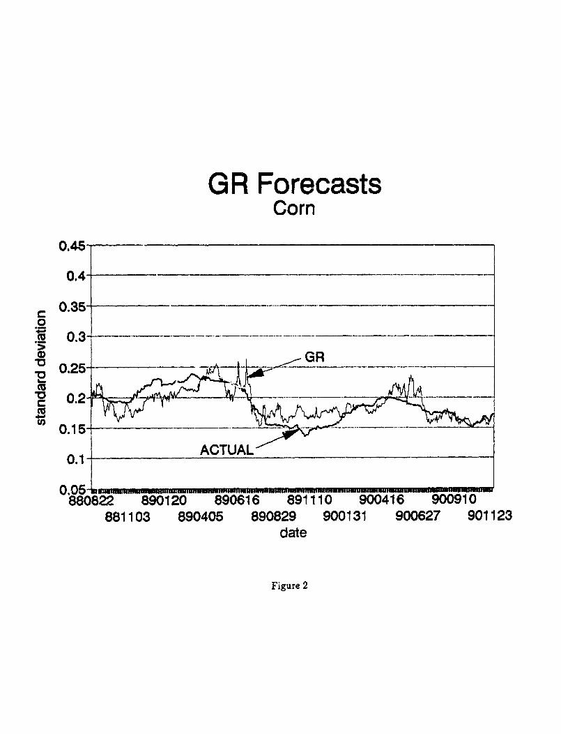
where the li's come from the in-sample regression (13). See Figure 2 for a graph of the GR forecast

for corn. In this figure, the first 406 observations (through February, 1990) were used to construct

the GR parameter estimates, meaning that this figure combines both in-sample and out-of-sample

forecasts. GR tracks the true volatility very well, increasing when actual volatility increases anddecreasing when actual volatility decreases. Unlike the COMB forecast, GR does not overpredict

high volatility periods and underpredict low volatility periods.

FIGURE 2

We now have seven forecasts of volatility. The first three (ISDAT, ISDAVG and ISD1) aremarket-based, the next two (HIST and GARCH) are time series based, and the final two (COMB

In order to compute the true volatility, we need 225 calendar days of returns, which translates into 160 working d1as%or 160 observations. Therefore, in order to make the Granger and Ramanathan forecasts truly out-of-sample, we nee,ito withhold 160 observations plus the 40 observations from the out-of-sample forecasting period, for 200 observatLw(n,Otherwise, the dependent variable in the Granger and Ramanathan regression would include some out-of-sample dAt

12 None of the conclusions of this paper are changed if the constant term is dropped from this regression,

14

and GR) combine the market and time series based forecasts. The results of the out-of-sample

MSFE are presented in Table 7. With the exception of cocoa and silver, the GR forecast has thelowest out-of-sample mean squared forecast error, and for silver the COMB forecast has the lowest.Also, the COMB forecast has the second-lowest MSFE for four of the five commodities where

GR has the lowest. The obvious conclusion is that the two combined forecasts perform better thaneither the time series forecasts or the market based forecasts. This suggests that much more precise

interval forecasts can be made using the GR or COMB forecasts of variance. Furthermore, since

the GR and COMB forecasts clearly dominate the ISD forecasts, we speculate that the difference

between the combined forecasts and the ISD forecasts can be used to identify mispriced options.

The idea is that since expectations of future volatility play such a critical role in the determination

of options prices, better forecasts of volatility should lead to better pricing and should therefore

help an investor identify over- or under-priced options contracts.

TABLE 7

VI. Conclusions.

The results presented above are promiEing. In particular, the COMB and GR forecasts, whichcombine market-based information with time series information, yield better forecasts than can beobtained from market expectations or time series models alone. Several implications of this areimmediately apparent. First, the time series contains information about future volatility that is notcaptured by market expectations, suggesting that options markets are inefficient (and/or the optionpricing formula we used is incorrect). This implies that it is possible that our volatility forecast canbe used to identify mispriced options, and a profitable trading rule could be established based onthe difference between the ISD and the COMB or GR volatility forecast. Second, our forecasting

method can be used to obtain interval forecasts of commodity prices, which should be beneficial tomarket participants who are concerned about the precision of a point forecast. One final note isthat the accurate matching of the forecast horizon and the time to maturity of the futures contract

is relatively unimportant. Our results indicate that near-maturity options tend to forecast long-runvolatility about as well as options that are far from maturity.

15

REFERENCES

Akigray, Vedat (1989), "Conditional Heteroskedasticity in Time Series Models of Stock Returns:Evidence and Forecasts," Journal of Business, 62, 55-99.

Barone-Adesi, Giovanni and Robert E. Whaley (1987), "Efficient Analytic Approximation of Amer-ican Option Values," Journal of Finance, 42, 301-320.

Bartunek, Kenneth and Chowdhury Mustafa (1991), "Forecasting the Variance of the UnderlyingAsset of an Option: A Comparison of Conditional and Unconditional Forecasts," unpublishedmanuscript, Louisiana State University.

Beckers, S. (1983), "Variances of Security Price Returns Based on High, Low and Closing Prites,"Journal of Business, 56, 97-112.

Black, Fisher (1976), 'The Pricing of Commodity Contracts," Journal of Financial Economics, 3,167-179.

Bolleralev, Tim, Ray Y. Chou and Kenneth F. Kroner (1992), "ARCH Modeling in Finance: AReview of the Theory and Empirical Evidence," Journal of Econometrics, 52, 5-60.

Cao, Charles Q. and Ruey S. Tsay (1991), "N- ullneb.r Time Series Analysis of Stock Volatilities,"unpublished manuscript, Graduate School of Business, University of Chicago.

Day, Theodore E. and Craig M. Lewis (1992), "Stock Market Volatility and the Information Contentof Stock Index Options," Journal of Econometrics, 52, 267-287.

Engle, Robert F. (1982), "Autoregressive Conditional Heteroskedasticity with Estimates of theVariance of U.K. Inflation," Econometrica, 50, 987-1007.

Engle Robert F. and Tim Bollerslev (1986), "Modeling the Persistence of Conditional Variances,"_conometric Reviews, 5, 1-50.

Granger, Clive W. and Ramu Ramanathan (1984), "Improved Methods of Combining Forecasts,"Journal of Forecasting, 3, 197-204.

Hull, John and Alan White (1987), "The Pricing of Options with Stochastic Volatility," Journal ofFinance, 42, 281-300.

Lamoureux, Christohper G. and William D. Lastrapes (1991), "Forecasting Stock Return Vari-ance: Toward an Understanding of Stochastic Implied Volatilities," unpublished manuscript,Washington University.

Latane, Henry A. and Richard J. Rendleman (1976), "Standard Deviations of Stock Price RatiosImplied in Option Prices," Journal of Finance, 31, 369-381.

Ramaswamy, Krishna and Suresh M. Sundaresan (1985), "The Valuation of American Options onFutures Contracts," Journal of Finance, 40, 1318-1340.

Taylor, Stephen J. (1987), "Forecasting the Volatility of Currency Exchange Rates," InternationalJournal of Forecasting, 3, 159-170.

Wei, Shang-Jin and Jeffrey A. Frankel (1991), "Are Option-Implied Forecasts of Exchange RateVolatility Excessively Variable?" unpublished manuscript, NBER Working Paper No. 3910.

16

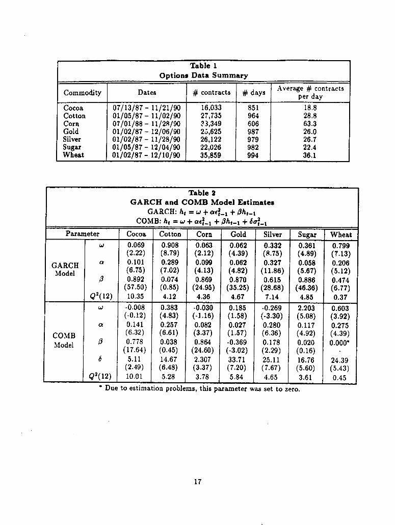
Table 1Options Data Summary

Commodity Dates # contracts # days per day

Cocoa 07/13/87 - 11/21/90 16,033 851 18.8Cotton 01/05/87 - 11/02/90 27,735 964 28.8Corn 07/01/88 - 11/28/90 23,349 606 63.3Gold 01/02/87 - 12/06/90 25,625 987 26.0Silver 01/02/87 - 11/28/90 26,122 979 26.7Sugar 01/05/87 - 12/04/90 22,026 982 22.4Wheat 01/02/87 - 12/10/90 35,859 994 36.1

Table 2GARCH and COMB Model Estimates

GARCH: ht = w + ad-_ + /ht-Xj_____________ COMB: ht = w + a.2_1 + 3ht-I + Mt_ _

Parameter Cocoa Cotton Corn Gold Silver Sugar Wheatw 0.069 0.908 0.063 0.062 0.332 0.361 0.799

(2.22) (8.79) (2.12) (4.39) (8.75) (4.89) (7.13)GARCH a 0.101 0.289 0.099 0.062 0.327 0.058 0.206Model (6.75) (7.02) (4.13) (4.82) (11.86) (5.67) (5.12)

,3 0.892 0.074 0.869 0.870 0.615 0.886 0.474(57.50) (0.85) (24.95) (35.25) (28.68) (46.36) (6.77)

_________ Q2 (12) 10.35 4.12 4.36 4.67 7.14 4.85 0.37w S -0.008 0.383 -0.030 0.185 -0.269 2.203 0.603

(-0.12) (4.83) (-1.16) (1.58) (-3.30) (5.08) (3.92)at 0.141 0.257 0.082 0.027 0.280 0.117 0.275

COMB (6.32) (6.61) (3.37) (1.57) (6.36) (4.92) (4.39)Model 0.778 0.038 0.864 -0.369 0.178 0.020 0.0000(17.64) (0.45) (24.60) (-3.02) (2.29) (0.16)

6 5.11 14.67 2.307 33.71 25.11 16.76 24.39(2.49) (6.48) (3.37) (7.20) (7.67) (5.60) (5.43)

Q2(12) 10.01 5.28 3.78 5.84 4.65 3.61 0.45Due to estimation problems, this parameter was set to zero.

17

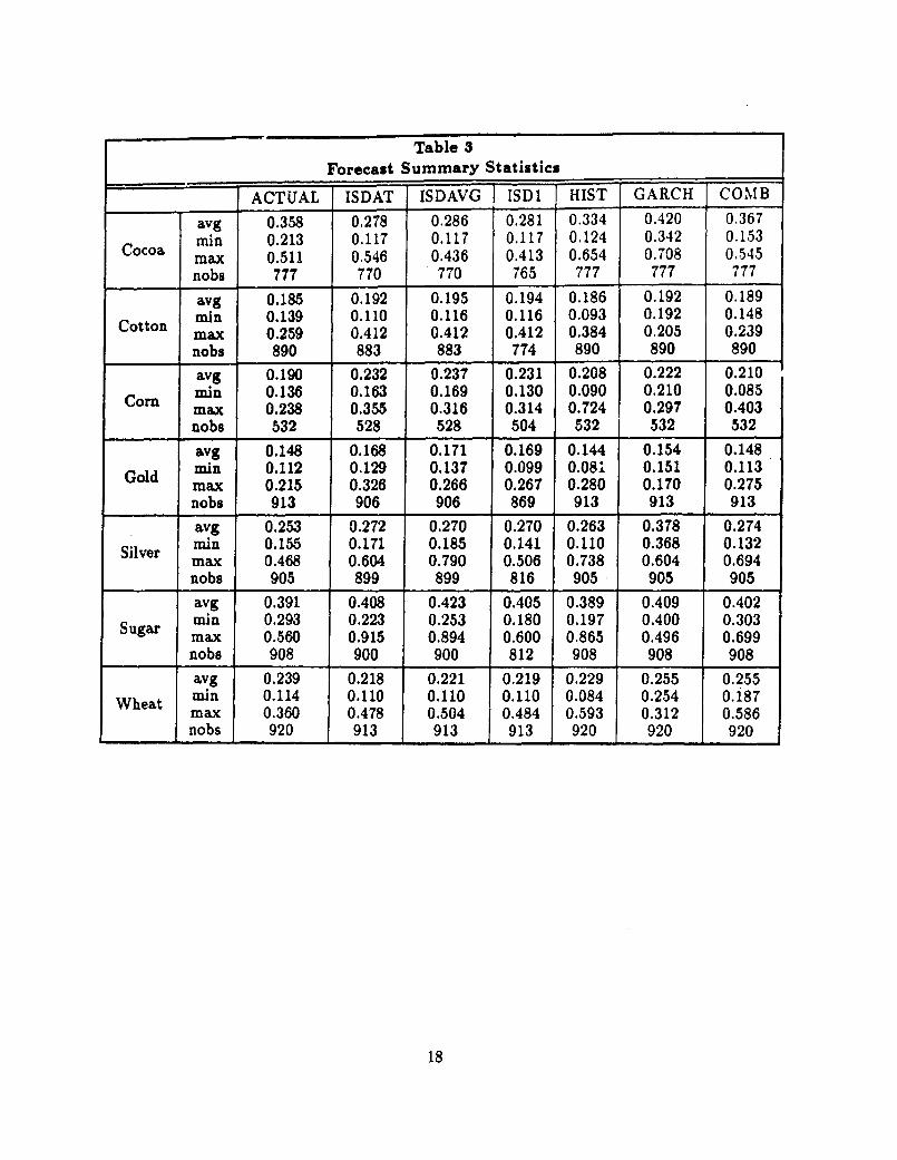
Table 3Forecast Summary Statistics

ACTUAL ISDAT ISDAVG ISD1 HIST GARCH COMBavg 0.358 0.278 0.286 0.281 0.334 0.420 0.367min 0.213 0.117 0.117 0.117 0.124 0.342 0.153Cocoa max 0.511 0.546 0.436 0.413 0.654 0.708 0.545nobs 777 770 770 765 777 777 777avg 0.185 0.192 0.195 0.194 0.186 0.192 0.189min 0.139 0.110 0.116 0.116 0.093 0.192 0.148

Cotton max 0.259 0.412 0.412 0.412 0.384 0.205 0.239nobs 890 883 883 774 890 890 890avg 0.190 0.232 0.237 0.231 0.208 0.222 0.210

Corn rain 0.136 0.163 0.169 0.130 0.090 0.210 0.085max 0.238 0.355 0.316 0.314 0.724 0.297 0.403nobs 532 528 528 504 532 532 532avg 0.148 0.168 0.171 0.169 0.144 0.154 0.148min 0.112 0.129 0.137 0.099 0.08; 0.151 0.113

Gold max 0.215 0.326 0.266 0.267 0.280 0.170 0.275nobs 913 906 906 869 913 913 913avg 0.253 0.272 0.270 0.270 0.263 0.378 0.274

Silver min 0.155 0.171 0.185 0.141 0.110 0.368 0.132max 0.468 0.604 0.790 0.506 0.738 0.604 0.694nobs 905 899 899 816 905 905 905avg 0.391 0.408 0.423 0.405 0.389 0.409 0.402

Sugar min 0.293 0.223 0.253 0.180 0.197 0.400 0.303Sugar max 0.560 0.915 0.894 0.600 0.865 0.496 0.699

nobs 908 900 900 812 908 908 908avg 0.239 0.218 0.221 0.219 0.229 0.255 0.255

Wheat min 0.114 0.110 0.110 0.110 0.084 0.254 o.187max 0.360 0.478 0.504 0.484 0.593 0.312 0.586nobs 920 913 913 913 920 920 920

18

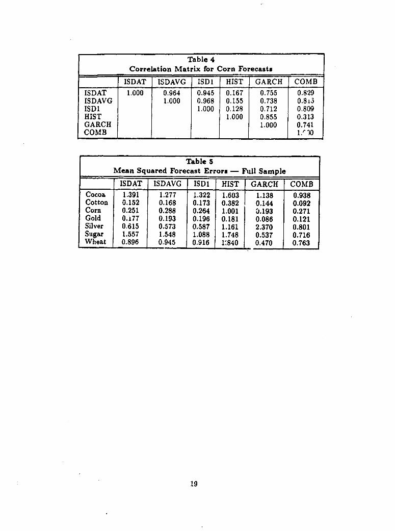
Table 4Correlation Matrix for Corn Forecasts

ISDAT ISDAVG ISD1 HIST GARCH COMBISDAT 1.000 0.964 0.945 0.167 0.755 0.829ISDAVG 1.000 0.968 0.155 0.738 0.813ISD1 1.000 0.128 0.712 0.809HIST 1.000 0.855 0.313GARCH 1.000 0.741COMB 19 10

Table 5Mean Squared Forecast Errors - Full Sample

ISDAT ISDAVG ISD1 HIST GARCH COMB

Cocoa 1.391 1.277 1.322 1.603 1.138 0.938Cotton 0.152 0.168 0.173 0.382 0.144 0.092Corn 0.251 0.288 0.264 1.001 0.193 0.271Gold 0.i77 0.193 0.196 0.181 0.086 0.121Silver 0.615 0.573 0.587 1.161 2.370 0.801Sugar 1.557 1.548 1.088 1.748 0.537 0.716Wheat 0.896 0.945 0.916 1:840 0.470 0.763

19

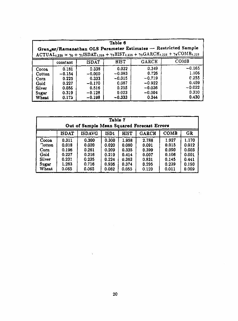
Table 6Gran,er/Ramanathan OLS Parameter Estimates - Restricted Sample

ACTUAL9,225 = -Yo + j'IISDATt,225 + Y2HISTt,225 + 'y3GARCHt,225 + I 4COMBf.22 5

constant ISDAT HIST GARCH COMB

Cocoa 0.181 0.338 0.032 0.349 -0.165Cotton -0.154 -0.000 -0.083 0.726 1.106Corn 0.225 0.333 -0.015 -0.719 0.255Gold 0.227 -0.170 C.087 -0.922 0.409Silver 0.056 0.516 0.255 -0.036 -0.022Sugar 0.319 -0.128 0.023 -0.004 0.310Wheat 0.173 -0.198 -0.333 0.344 0.430

Table 7Out of Sample Mean Squared Forecast Errors

1 ISDAT ISDAVG ISDI HIST GARCH COMB GR

Cocoa 0.311 0.300 0.300 1.958 2.788 1.927 1.170cotton 0.018 0.020 0.020 0.080 0.091 0.015 0.012Corn 0.196 0.261 0.209 0.335 0.399 0.090 0.003Gold 0.227 0.216 0.219 0.414 0.007 0.106 0.001Silver 0.231 0.235 0.224 0.363 0.831 0.145 0.441Sugar 1.283 0.716 0.936 0.374 0.295 0.239 0.190Wheat 0.065 0.065 0.062 0.055 0.120 0.011 0.009

20

ISDAT Forecasts HIST ForecastsCorn Corn

0.45 0.45-

0.41 - 1 0.4-

0.35 0.35-

. o I ,. ISOAT ! °|u 0.2 ji STm

0.2- ~~~~~~~~~~~~~~~~~~~0.2-~~~~~~~~~~~~~~~~~~~~~~~~~~~~~~~~~~~~~~~~~~~~~~~~~~~~~~~~~~~~~~~~~~~~~~~

U, Urn .15

0-1ACT6lAL ACTUAL '>-0.15-

0.15 0.1588C322 890120 890616 891110 900416 900910 880E22 890120 890616 891110 900416 900910881103 890405 890829 900131 900627 90t123 881103 890405 890829 900 'I 900627 901123

date date

GARCH Forecasts COMB ForecastsCorn Com

0.45 0.45

0.4- 0.4

0.35 c0.35-i l

u- 03- GUC 0.3- COlD Bl

0.2 0~~~~~~~~~~~~~~~~~~~~~~~.2 -,0 2;5 H < ,15 <

0.1- ACTnUAL |ACTUAL0.1~

0.05' ~~~~~~~~~~~~~~~~~~~~0.05'880622 890120 890616 891110 900416 900910 880e22 890120 890616 891110 900416 900910

881103 890405 890829 900131 900627 901123 881103 890405 890629 900131 900627 901123date date

Figure 1

GR ForecastsCorn

0.45-

0.4-

0.35-0

______ ~~GR_ _

0.25-

0.2--

0.1 5-__.__ _.... _

ACTUALL0.15-_

8808B22 890120 890616 891110 900416 900910881103 890405 890829 900131 900627 901123

date

Figure 2

Policy Research Working Paper Series

ContactTltle Author Date for paper

WPS1208 Primary School Achievernent in Levi M. Nyagura Octoher 1993 I. ConachyEnglish and Mathematics in Abby Riddell 33669ZimbaLrwe: A Mu!ti-Level Analysis

WPS1209 Should East Asia Go R9egional'7 Arvind Panagariya October 1993 D. BallantyneNo, No, and Maybe 37947

WPS1210 The Taxation of Natural Resources. Robin Boauway October 1993 C. JonesPrinciples and Policy Issues Frank Flatters 37699

WPS121 1 Savings-Investment Correlations Nlandu Mamingi October 1993 R. Voand Capital Mobility in Developing Countries 31047

WPS1212 The Links between Economic Policy Ravi Kanbur October 1993 P. Attipoeand Research: Three Exarmiples from 526-3003Ghana and Some General Thoughts

WPS1213 Japanese Foreign Direct Investment: Kwang W. Jun November 1993 S. King-WatsonRecent Trends, Determinants, and Frank Sader 33730Prospects Haruo Horaguchi

Hyuntai Kwak

WPS1214 Trade, Aid, and Investrnent in Sub- Ishrat Husain November 1993 M. YoussefSaharan Africa 34637

WPS1215 How Much Do Distortions Affect W,ll am Easterly November 1993 R. MarlinG rowth9 39065

WPS1216 Regulation, Institutons, and Alice Hll November 1993 D. EvansCommitment: Privatizt on and MaEr.el Angel Abdaia 38526Regulation in the AraniineTelecommuriications Sector

WPS1217 Unitary versus Collective Models Pierre-Andre Chiappori November 1993 P. Attipoeof the Household: Time to Shift the Lawrence Haddad 526-3002Burden of Proof? John Hoddinott

Ravi Kanbur

WPS1218 Implementation of Trade Reform in John Nash November 1993 D. BallantyneSub-Saharan Africa: How Much Heat 37947and How Much Light?

WPS1219 Decentralizing Water Resource K. Wh!liam Easte, November 1993 M. WuManagement: Economic Incentives, Robert R. Hearne 30480Accountability, ana Assurance

WPS1220 Developing Countries and *he Bernard Hoekman Nconmber 1993 L. O'ConnorUruguay Round: Negotiations on 37009Services

Policy Research Working Paper Series

Contac:Title Author Date for paper

WPS1221 Does Research and Development Nancy Birdsall November 1993 S. RajanContribute to Economic Growth Clhangyong Rhee 33747in Developing Cour.,ries'?

WPS1222 Trade Reform in Ten Sub-Saharan Faezeh Foroutan November 1993 S. FallonCountries: Achievements and Failures 38009

WPS1223 How Robust Is a Poverty Profile? Martin Ravallion November 1993 P. CookBenu Bidani 33902

WPS1224 Devaluation in Low-inflation Miguel A. Kiguel November 1993 R. LuzEconomies Nita Ghei 39059

WPS1225 Intra-Sub-Saharan African Trade: Faezeh Foroutan Nnvember 1993 S. FallonIs It Too Little? Lant Pritchett 38009

WPS1226 Forecasting Volatility in Commodity Kenneth F, Kroner November 1993 F. HatabMarkets Devin P. Kneafsey 35835

Stijn Claessens