forecasting volatility - diva portal304496/fulltext01.pdf · forecasting volatility volatility...

Forecasting volatility

Richard Minkah

U.U.D.M. Project Report 2007:7

Examensarbete i matematik, 20 poäng

Handledare och examinator: Maciej Klimek

Februari 2007

Department of Mathematics

Uppsala University

i

Dedications

To the almighty God, Jesus Christ and the Holy Spirit for the guidance and care.

To my cherished Mum, Agnes Owusu and Uncle F.K. Owusu.

You provided me with parental care and financial support to ensure my pursuit for

higher education become real.

To Miss Theodora Donkor.

Though you were far away, your persistent telephone calls and the thought of you gave

me the enthusiasm to carry on with my academic work.

ii

Acknowledgement

I am especially grateful to my supervisor Professor Maciej Klimek for his helpful

comments, suggestions and corrections towards the realization of this work.

I am also indebted to all the lecturers who taught me in the entire program especially

Dag Jonsson, Professor Johan Tysk, Professor Ingemar Kaj and Silvelyn Zwanzig.

I am also thankful to Mr Ernest Amartey-Vondee and Rev. Ernest Koranteng for their

material support.

Finally, I wish to express heartfelt thanks to my course mates, Bernard Mawah and

Francis Atsu for your help and encouragement throughout my stay in Sweden.

iii

Abstract

FORECASTING VOLATILITY

Volatility plays a very important role in any financial market around the world.

Accurate forecasting of volatility is essential for asset and derivative pricing models

and other financial applications. The goal of any volatility model is to be able to

forecast volatility. In this paper, we examine the forecasting ability of three widely

used time series volatility models namely, the Historical Variance, The Generalized

AutoRegressive Conditional Heteroscedastic (GARCH) Model and the RiskMetrics

Exponential Weighted Moving Average. The characteristics of these volatility models

are explored using data on the Standard &Poor’s (S&P) 500 Index, Dow Jones

Industrial Average (DJIA), OMX Swedish Stock Exchange (OMXS30) index, Dow

Jones-AIG Commodity Index (DJ-AIGCI), The 3 Months US Treasury Bill Yield and

the Ghanaian Cedi and the US Dollar (CEDI/USD) exchange rate.

Keywords: Exponentially weighted Moving Average; GARCH; Historical Variance;

Volatility

Examiner: Professor Maciej Klimek

iv

Table of Contents

Dedications............................................................................................................. i

Acknowledgement.................................................................................................. ii

Abstract................................................................................................................... iii

List of Tables.......................................................................................................... vi

List of figures......................................................................................................... vii

1 Introduction………………………………………………………………. 1

2 Time Series Concept……………………………………………………… 3

2.1 Stationarity………………........…………………………………… 3

2.1.1 Nonstationarity…........……………………………………. 5

2.2 Autocorrelation………................…………………………………. 5

2.2.1 The Ljung-Box Q-Statistics……………………………….. 6

3 Statistical and Probability Foundations………………………………… 8

3.1 Financial Price Changes and returns………………………………. 8

3.1.1 Return Aggregation………………………………………... 9

3.2 Modelling financial prices and returns...…………………………... 10

4 Volatility Modelling and Forecasting........................................................ 12

4.1 Historical Variance........................................................................... 13

4.2 The RiskMetrics’ Exponential Weighted Moving

Average………………………………………….………………... 14

4.2.1 Estimating the Parameters of the RiskMetrics

Model……………………………………………………… 16

4.2.2 Determining the Decay Factor ……………………………. 17

4.3 The Generalized Autoregressive Conditional

Heteroscedastic (GARCH) model………………………………… 17

4.3.1 Estimation of the GARCH(1,1) Model. .............................. 18

4.3.2 The GARCH(1,1) k-Period Volatility Forecast.................... 19

4.4 Measuring Forecasting Performance................................................ 20

5 Data Analysis............................................................................................... 22

5.1 Description of Data………………………………………………. 22

5.2 Fitting the GARCH(1,1) Model...................................................... 28

5.3 Fitting the RiskMetrics Exponential Weighted Moving Average

(EWMA).......................................................................................... 43

5.4 Comparing the Volatility Models.................................................... 50

5.5 Conclusions……………………………………………………….. 56

References 57

v

Appendix

A.1 Aggregation Property of the Normal Distribution............................ 58

A.2 Test for Conditional Normality.….…………............……....…...... 58

A.3 The RiskMetrics k-period (day) Volatility Forecast......................... 59

vi

List of Tables

5.1 summary statistics of the returns…………………………………………. 28

5.2 Ljung-Box Q test for returns……………………………………………... 35

5.3 Ljung-Box Q test for squared returns…………………………………….. 35

5.4 Estimated parameters of the GARCH(1,1) model for various return

series............................................................................................................ 36

5.5 Unconditional mean and volatility estimates of the GARCH(1,1)............. 36

5.6 Ljung-Box Q-Statistics for squared standardised residuals using

GARCH(1,1)............................................................................................... 36

5.7 RiskMetrics volatility Estimates................................................................. 43

5.8 Ljung-Box Q-Statistics for squared standardized residuals using

RiskMetrics EWMA …............................................................................... 50

5.9 In-Sample Root Mean Squared Forecast Errors of the volatility models.... 50

5.10 Out-Sample Root Mean Squared Forecast Errors for a 20-day Forecasting

Horizon......................................................................................................... 55


Horizon......................................................................................................... 55


Horizon......................................................................................................... 56

vii

List of Figures

2.1 Simulated stationary time series…………………………………………… 4

2.2 A non-stationary time series of SEK/CEDI foreign exchange rate………. 5

2.3 Plot of a sample autocorrelation coefficients for SEK/CEDI foreign

exchange rate……………………………………………………………… 6

5.1 Time series plots of S&P500, DJIA and the OMXS30 index..................... 23

5.2 Time series plots of DJ-AIGCI, 3 Months US T-Bill and CEDI/USD

Exchange rate............................................................................................. 24

5.3 Plots of returns for the S&P500, DJIA and the OMXS30.......................... 26

5.4 Plots of returns for the DJ-AIGCI, 3 Months US Treasury Bill and the

CEDI/USD.................................................................................................. 27

5.5 Normal probability plot of the returns of the S&P500, DJIA, and the

OMXS30.................................................................................................... 29

5.6 Normal probability plot of the returns of the DJ-AIGCI, 3 Months US

Treasury Bill, CEDI/USD......................................................................... 30

5.7 Plots of autocorrelation coefficients for the returns of the S&P500,

DJIA and OMXS30................................................................................... 31

5.8 Plots of autocorrelation coefficients for the returns of the DJ-AIGCI,

3 Months US T-Bill, CEDI/USD............................................................ 32

5.9 Plots of autocorrelation coefficients for the squared returns of the

S&P500, DJIA and the OMXS30............................................................. 33

5.10 Plots of autocorrelation coefficients for the squared returns of the

DJ-AIGCI, 3 Months US Treasury Bill and CEDI/USD......................... 34

5.11 Estimated conditional volatility using GARCH(1,1) for the S&P500,

DJIA and OMXS30................................................................................. 37

5.12 Estimated conditional volatility using GARCH(1,1) for the DJ-AIGCI,

3 Months US T-Bill and CEDI/USD........................................................ 38

5.13 Plot of the standardised residuals for S&P500, DJIA and OMXS30

using GARCH(1,1)................................................................................... 39

5.14 Plot of the standardised residuals for DJ-AIGCI, 3 Months US T-Bill

and CEDI/USD using GARCH(1,1).......................................................... 40

5.15 Plots of autocorrelation coefficients for the squared standardised

residuals for S&P500, DJIA and OMXS30 using GARCH(1,1).............. 41


residuals for the DJ-AIGCI, 3 Months US T-Bill and CEDI/USD

using GARCH(1,1)...................................................................................... 42

5.17 Plot of estimated conditional volatility using RiskMetrics EWMA for the

S&P500, DJIA and OMXS30.................................................................... 44

5.18 Plot of estimated volatility using RiskMetrics EWMA model for the DJ-

AIGCI, 3 Months US T-Bill and CEDI/USD............................................ 45

5.19 Normal probability plots for the standardised residuals of the S&P500,

DJIA and OMXS30 using RiskMetrics EWMA model............................. 46

5.20 Normal probability plots for the standardised residuals of the DJ-AIGCI,

3 Months US T-Bill and CEDI/USD using RiskMetrics EWMA model.... 47

5.21 Plots of autocorrelation coefficients for the squared standardised residuals

for the S&P500, DJIA and OMXS30 using RiskMetrics EWMA model… 48


residuals for the DJ-AIGCI, 3 Months US T-Bill and CEDI/USD using

RiskMetrics EWMA model………………………....................................... 49

viii

5.23 GARCH(1,1) and EWMA estimators on the S&P500, DJIA and

OMXS30 return series.......................................................................... 51

5.24 GARCH(1,1) and EWMA estimators on the DJ-AIGCI, 3 Months

US T-Bill and CEDI/USD return series.................................................. 52

5.25 Volatility Forecast on S&P500, DJIA and OMXS30 return series......... 53

5.26 Volatility Forecast on DJ-AIGCI, 3 Months US T-Bill and CEDI/USD

return series............................................................................................ 54

1

Chapter 1

Introduction

Volatility has become an indispensable topic in financial markets for risk managers,

portfolio managers, investors, academicians and almost all that have something to do

with the financial markets. Forecasting accurately future volatility and correlations of

financial asset returns is essential to derivatives pricing, optimal asset allocation,

portfolio risk management, dynamic hedging and as an input for Value-at-Risk

models.

The importance of volatility forecasting was highlighted when in 2003 Professor R.F

Engle was awarded a Noble price for his outstanding contribution in modelling

volatility dynamics.

“The advantage of knowing about risks is that we can change our behaviour to avoid

them. Of course, it is easily observed that to avoid all risks would be impossible; it

might entail no flying, no driving, no walking, eating and drinking only healthy foods

and never being touched by sunshine. Even a bath could be dangerous. I could not

receive this prize if I sought to avoid all risks. There are some risks we choose to take

because the benefits from taking them exceed the possible costs. Optimal behaviour

takes risks that are worthwhile. This is the central paradigm of finance; we must take

risks to achieve rewards but not all risks are equally rewarded. Both the risks and the

rewards are in the future, so it is the expectation of loss that is balanced against the

expectation of reward. Thus we optimize our behaviour, and in particular our

portfolio, to maximize rewards and minimize risks”1.

Volatility has a central role in the derivatives pricing theory. The Black-Scholes model

has volatility as the only parameter among strike price, time to expiration, interest rate,

and strike price that has to be forecasted. The underlying assets’ volatility is needed in

the pricing of an option and there are options with volatility as the underlying assets.

The 1996 and 1999 Basel Accord makes it compulsory for financial institutions to

incorporate financial risk exposure in calculating the basic capital requirements. This

makes volatility forecasting an obligatory task for all financial institutions.

Volatility and correlations are estimated from historical data on asset returns or from

observed option prices since it cannot be observed directly. Any volatility model

should be able to forecast volatility. Time series models are used on historical data on

asset returns to forecast volatility and correlations whiles implied volatility uses

observed option prices.

The common assumed model for logarithmic returns of an asset is the (Multi) normal

distribution. Real data from the financial markets have being found to violate this

assumption, with the leptokurtotic (fat-tailed) a more appealing distribution. The non-

stationarity in the financial market data introduces some complication in the

variance/covariance matrix forecasting. In this work, we focus on three time series

models for estimating volatility namely Historical Variance, Exponential Weighted

1 Engle 2003, Noble Lecture, page 326

2

Moving Average (EWMA) and the Generalised AutoRegressive Moving Average

(GARCH). We investigate the forecasting ability of these three models.

The paper is organised as follows. In chapter 2, we explore the concept of time series,

including definitions, stationarity and autocorrelations. In chapter 3, we will describe

the statistical and probability foundations underpinning the various volatility models.

This involves description of financial price changes, return aggregation and the

modelling of the price changes. We then introduce the volatility models namely, the

Historical Variance, The RiskMetrics Exponential Weighted Moving Average and the

Generalised Autoregressive Conditional Heteroscedastic. Finally, in chapter 5, we fit

the Standard & Poor’s (S&P) 500 Stock Price Index, Dow Jones Industrial Average

(DJIA), OMXS30 Stock Price Index, Dow Jones-AIG Commodity Index (DJ-AIGCI),

3 Months US Treasury Bill Yield and the Ghanaian Cedi and the US Dollar Exchange

Rate (CEDI/USD) by the various models. We will perform some diagnostics on the

fits. The In-Sample and Out-of-Sample forecasting ability of the various models are

compared and we make our conclusions.

3

Chapter 2

Time Series Concept

A time series is a set of observations { , 0, 1, 2,...}tx t = ± ± , each one being recorded at a

specific time t. There are two kinds of time series data namely discrete-time and

continuous-time series. In a discrete-time time series, the set of times at which

observations are made is discrete, as is the case for example, when observations are

made at fixed time intervals. However, in a continuous-time series, observations are

recorded continuously over some time interval, e.g. [0,1].

An important part of time series analysis is the selection of a suitable probability

model for the data. A time series model for observed data { tx } is a specification of a

stochastic process { tX } of which { tx } is postulated to be a realization. The term time

series is also used with respect to the stochastic process { tX }.

2.1 Stationarity

Stationarity has two forms namely (weak) stationarity and strict stationarity.

In simple terms, a time series { tX } is said to be stationary if it has statistical property

similar to those of the “time shifted” series { t hX + }, for each integer h and t∈ℤ .

Definition 2.1 (The joint distribution function)

The joint distribution function of random variables 1 2, ..., TX X X is given by

1 2, ,..., 1, 2 1 1 2 2( ,... ) ( , ..., )TX X X T T TF x x x P X x X x X x= ≤ ≤ ≤ (1)

where 1, 2 ,... Tx x x ∈ℝ .

Definition 2.2 (The mean function)

Let { }tX X= be a time series. The mean function of { tX } is

( ) ( )X tt E Xµ = , (2)

where ( )E is the mathematical expectation.

Definition 2.3 (The covariance function)

The covariance function is computed to give a summary of the dependence between

any two random variables used in modelling a time series. The covariance function of

a time series { }tX with variance ( )tVar X < ∞ is given by

4

( , ) [( ( ))( ( ))]X s X t Xcov s t E X s X tµ µ= − − (3)

for all integers s and t.

Definition 2.4 (Stationarity )

The time series { }tX is said to be (weakly) stationary if it has a finite variance,

constant first moment (mean), and is such that the cov( , )s t depends only on ( )t s− i.e.

(a) 2( ) ,tE X t< ∞ ∀

(b) ( ) ,tE X tµ= ∀

(c) cov ( , ) cov ( , ), , ,X Xs t s h t h s t h= + + ∀

where , ,s t h belongs to the set of integers.

Definition 2.5 (Strict stationarity)

The time series { }tX is said to be strictly stationary if the

joint distribution of 1 2

( , ,..., )pt t tX X X is the same as that of

1 2( , ,..., )

pt h t h t hX X X+ + + for

any choice of time instances 1 2, ,..., pt t t and any increment h.

21-Mar-1994 10-May-1994 29-Jun-1994 18-Aug-1994-0.25

-0.2

-0.15

-0.1

-0.05

0

0.05

0.1

0.15

0.2

0.25

Simulated Stationary TimeSeries

dates

Returns

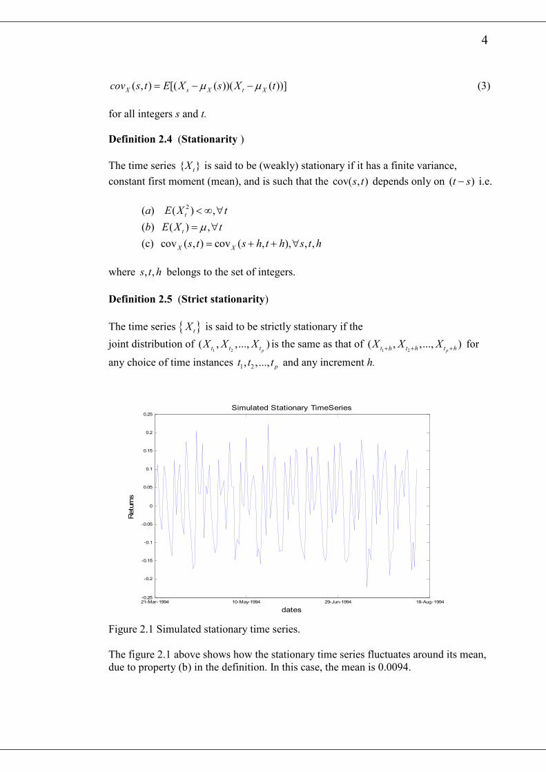
Figure 2.1 Simulated stationary time series.

The figure 2.1 above shows how the stationary time series fluctuates around its mean,

due to property (b) in the definition. In this case, the mean is 0.0094.

5

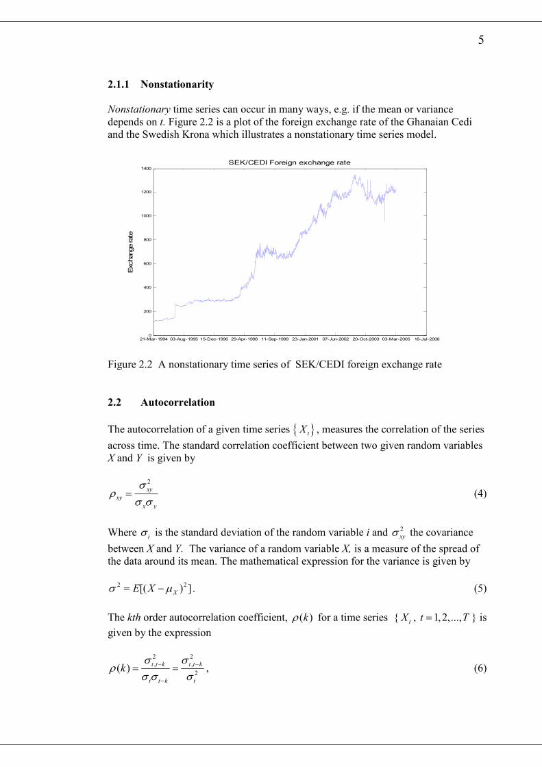
2.1.1 Nonstationarity

Nonstationary time series can occur in many ways, e.g. if the mean or variance

depends on t. Figure 2.2 is a plot of the foreign exchange rate of the Ghanaian Cedi

and the Swedish Krona which illustrates a nonstationary time series model.

21-Mar-1994 03-Aug-1995 15-Dec-1996 29-Apr-1998 11-Sep-1999 23-Jan-2001 07-Jun-2002 20-Oct-2003 03-Mar-2005 16-Jul-20060

200

400

600

800

1000

1200

1400

Exchange rate

SEK/CEDI Foreign exchange rate

Figure 2.2 A nonstationary time series of SEK/CEDI foreign exchange rate

2.2 Autocorrelation

The autocorrelation of a given time series { }tX , measures the correlation of the series

across time. The standard correlation coefficient between two given random variables

X and Y is given by

2

xy

xy

x y

σρ

σ σ= (4)

Where iσ is the standard deviation of the random variable i and 2

xyσ the covariance

between X and Y. The variance of a random variable X, is a measure of the spread of

the data around its mean. The mathematical expression for the variance is given by

2 2[( ) ]XE Xσ µ= − . (5)

The kth order autocorrelation coefficient, ( )kρ for a time series { tX , 1,2,...,t T= } is

given by the expression

2 2

, ,

2( )

t t k t t k

t t k t

kσ σ

ρσ σ σ

− −

−

= = , (6)

6

provided that we assume (weak) stationarity of { tX }. ( )kρ is normally estimated by

using a given sample of { tX }. Let { tx } be a given sample, then the estimate of the

autocorrelation coefficient at lag k is given by

{ }1

2

1

( )( ) /( 1)

ˆ( )

{( ) }/( 1)

T

t t k

t k

T

t

t

x x x x T k

k

x x T

ρ−

= +

=

− − − −=

− −

∑

∑ (7)

where 1

1 T

t

t

x xT =

= ∑ , the sample mean.

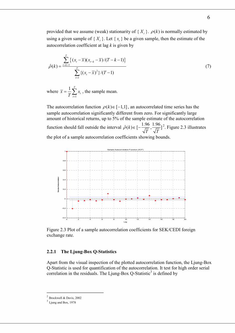
The autocorrelation function ( ) [ 1,1]kρ ∈ − , an autocorrelated time series has the

sample autocorrelation significantly different from zero. For significantly large

amount of historical returns, up to 5% of the sample estimate of the autocorrelation

function should fall outside the interval 1.96 1.96

ˆ( ) [ , ]kT T

ρ ∈ − 2. Figure 2.3 illustrates

the plot of a sample autocorrelation coefficients showing bounds.

0 2 4 6 8 10 12 14 16 18 20-0.4

-0.2

0

0.2

0.4

0.6

0.8

1

Lag

Sample Autocorrelation

Sample Autocorrelation Function (ACF)

Figure 2.3 Plot of a sample autocorrelation coefficients for SEK/CEDI foreign

exchange rate.

2.2.1 The Ljung-Box Q-Statistics

Apart from the visual inspection of the plotted autocorrelation function, the Ljung-Box

Q-Statistic is used for quantification of the autocorrelation. It test for high order serial

correlation in the residuals. The Ljung-Box Q-Statistic3 is defined by

2 Brockwell & Davis, 2002

3 Ljung and Box, 1978

7

2

1

( 2)h

j

j

Q n nn j

ρ

=

= +−∑ (8)

Where n is the number of observations, h is the largest lag and jρ is the sample

autocorrelation function at lag j, of an appropriate time series.

Under the null hypothesis that a times series is not autocorrelated, the Ljung-Box Q-

Statistic is distributed as chi-squared with h degrees of freedom.

8

Chapter 3

Statistical and Probability Foundations

In this section, we present the statistical and probability foundations upon which the

Historical Variance, RiskMetrics EWMA and the GARCH models are based on.

3.1 Financial Price Changes and returns

Price changes are often used as a measure of risk and a variety of these changes exist.

Among them are absolute, relative and log price changes. A return on a portfolio is a

price change defined relative to some initial price.

Let tP be the price of a security at date t, where t is usually taken as one business day

but can be a week or a month etc. The relative price change or percent return is

defined as

1

1

t tt

t

P PR

P

−

−

−=

(9)

If the gross return on a security is just1 tR+ , then the logarithmic return (or

continuously compounded return), tr , of a security is defined as

ln(1 )t tr R= +

1

1

ln t

t

t t

P

P

p p

−

−

=

= − (10)

where ln( )t tp P= is the natural logarithm of tP .

Returns are preferred over prices in this work because returns have more attractive

statistical properties than prices.

Similarly for multiple-day (k-days) horizon, the relative price change is defined as

,t t k

t t k

t k

P PR

P

−+

−

−= . (11)

The k-days gross return ,1 t t kR ++ can be expressed in terms of the 1-day returns as

, 1 2 11 (1 )(1 )(1 )...(1 )t t k t t t t kR R R R R+ − − − −+ = + + + +

1 2 1

1 2 3

. . ...t t t t k

t t t t k

P P P P

P P P P

− − − −

− − − −

= t

t k

P

P−

= (12)

9

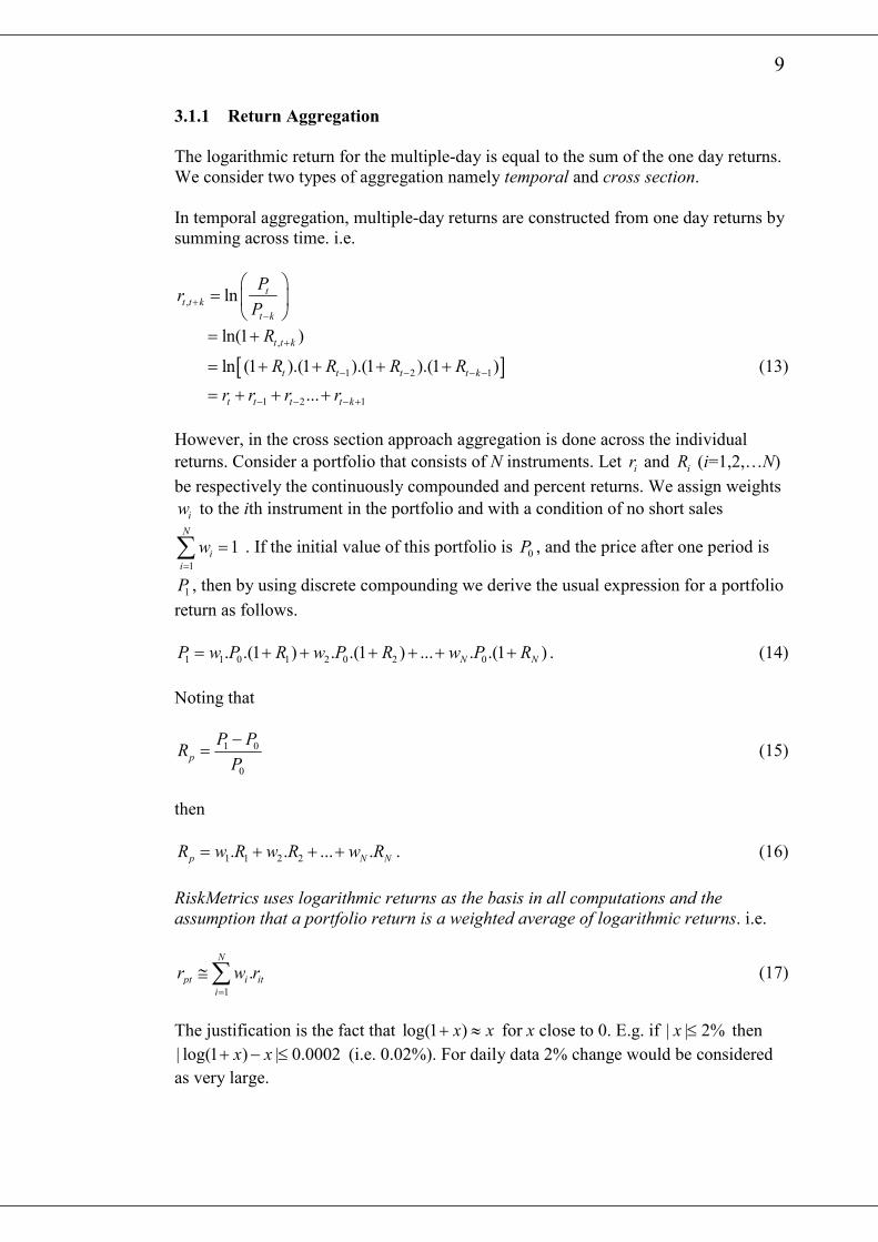
3.1.1 Return Aggregation

The logarithmic return for the multiple-day is equal to the sum of the one day returns.

We consider two types of aggregation namely temporal and cross section.

In temporal aggregation, multiple-day returns are constructed from one day returns by

summing across time. i.e.

, ln tt t k

t k

Pr

P+

−

=

[ ],

1 2 1

1 2 1

ln(1 )

ln (1 ).(1 ).(1 ).(1 )

...

t t k

t t t t k

t t t t k

R

R R R R

r r r r

+

− − − −

− − − +

= +

= + + + +

= + + +

(13)

However, in the cross section approach aggregation is done across the individual

returns. Consider a portfolio that consists of N instruments. Let ir and iR (i=1,2,…N)

be respectively the continuously compounded and percent returns. We assign weights

iw to the ith instrument in the portfolio and with a condition of no short sales

1

1N

i

i

w=

=∑ . If the initial value of this portfolio is 0P , and the price after one period is

1P , then by using discrete compounding we derive the usual expression for a portfolio

return as follows.

1 1 0 1 2 0 2 0. .(1 ) . .(1 ) ... . .(1 )N NP w P R w P R w P R= + + + + + + . (14)

Noting that

1 0

0

p

P PR

P

−= (15)

then

1 1 2 2. . ... .p N NR w R w R w R= + + + . (16)

RiskMetrics uses logarithmic returns as the basis in all computations and the

assumption that a portfolio return is a weighted average of logarithmic returns. i.e.

1

.N

pt i it

i

r w r=

≅∑ (17)

The justification is the fact that log(1 )x x+ ≈ for x close to 0. E.g. if | | 2%x ≤ then

| log(1 ) | 0.0002x x+ − ≤ (i.e. 0.02%). For daily data 2% change would be considered

as very large.

10

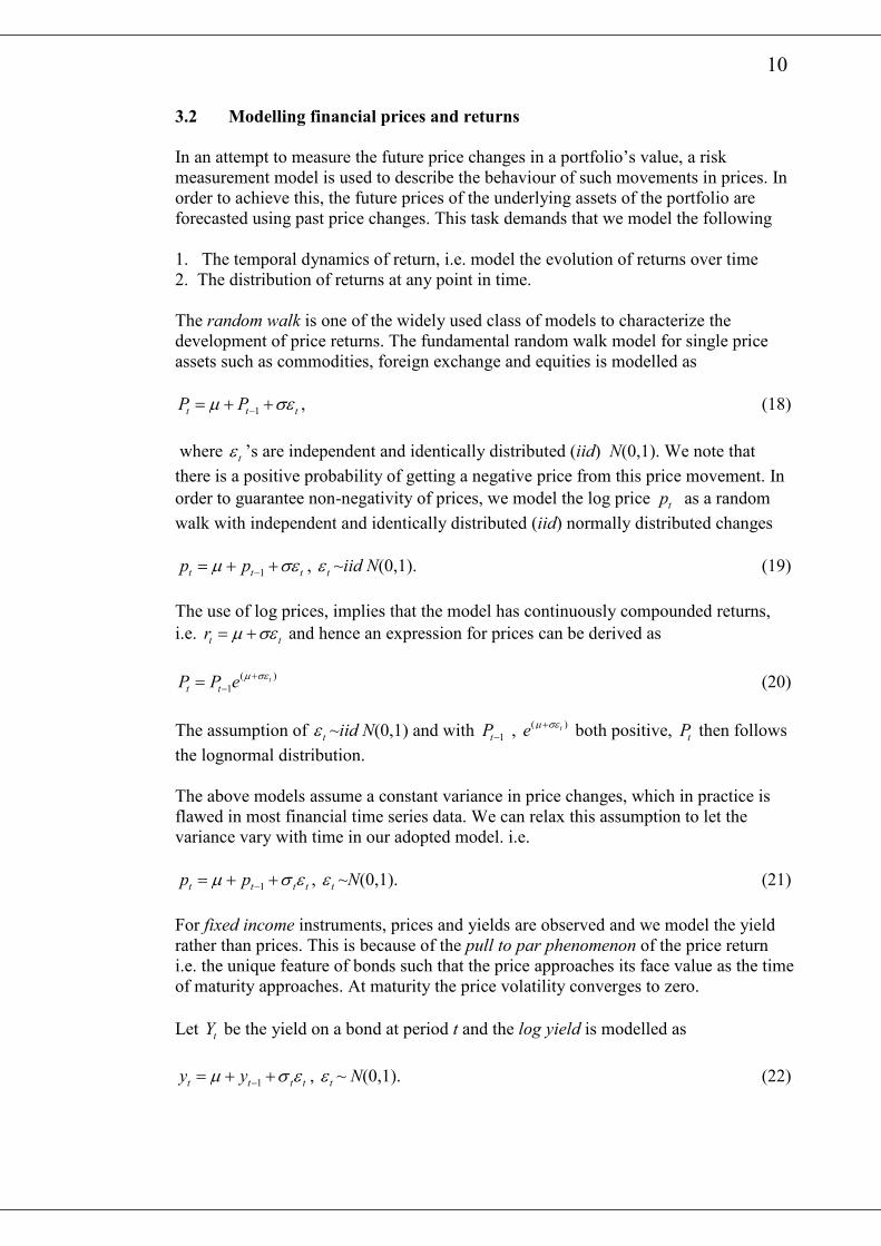
3.2 Modelling financial prices and returns

In an attempt to measure the future price changes in a portfolio’s value, a risk

measurement model is used to describe the behaviour of such movements in prices. In

order to achieve this, the future prices of the underlying assets of the portfolio are

forecasted using past price changes. This task demands that we model the following

1. The temporal dynamics of return, i.e. model the evolution of returns over time

2. The distribution of returns at any point in time.

The random walk is one of the widely used class of models to characterize the

development of price returns. The fundamental random walk model for single price

assets such as commodities, foreign exchange and equities is modelled as

1t t tP Pµ σε−= + + , (18)

where tε ’s are independent and identically distributed (iid) N(0,1). We note that

there is a positive probability of getting a negative price from this price movement. In

order to guarantee non-negativity of prices, we model the log price tp as a random

walk with independent and identically distributed (iid) normally distributed changes

1t t tp pµ σε−= + + , tε ~iid N(0,1). (19)

The use of log prices, implies that the model has continuously compounded returns,

i.e. t tr µ σε= + and hence an expression for prices can be derived as

( )

1t

t tP P eµ σε+

−= (20)

The assumption of tε ~iid N(0,1) and with 1tP− , ( )teµ σε+

both positive, tP then follows

the lognormal distribution.

The above models assume a constant variance in price changes, which in practice is

flawed in most financial time series data. We can relax this assumption to let the

variance vary with time in our adopted model. i.e.

1t t t tp pµ σ ε−= + + , tε ~N(0,1). (21)

For fixed income instruments, prices and yields are observed and we model the yield

rather than prices. This is because of the pull to par phenomenon of the price return

i.e. the unique feature of bonds such that the price approaches its face value as the time

of maturity approaches. At maturity the price volatility converges to zero.

Let tY be the yield on a bond at period t and the log yield is modelled as

1t t t ty yµ σ ε−= + + , tε ~ N(0,1). (22)

11

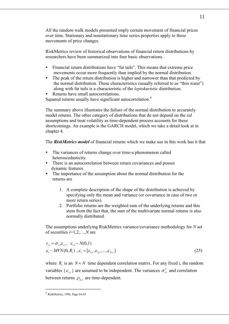
All the random walk models presented imply certain movement of financial prices

over time. Stationary and nonstationary time series properties apply to these

movements of price changes.

RiskMetrics review of historical observations of financial return distributions by

researchers have been summarized into four basic observations.

� Financial return distributions have “fat tails”. This means that extreme price

movements occur more frequently than implied by the normal distribution.

� The peak of the return distribution is higher and narrower than that predicted by

the normal distribution. These characteristics (usually referred to as “thin waist”)

along with fat tails is a characteristic of the leptokurtotic distribution.

� Returns have small autocorrelations.

Squared returns usually have significant autocorrelation.4

The summary above illustrates the failure of the normal distribution to accurately

model returns. The other category of distributions that do not depend on the iid

assumptions and treat volatility as time-dependent process accounts for these

shortcomings. An example is the GARCH model, which we take a detail look at in

chapter 4.

The RiskMetrics model of financial returns which we make use in this work has it that

� The variances of returns change over time-a phenomenon called

heteroscedasticity.

� There is an autocorrelation between return covariances and posses

dynamic features.

� The importance of the assumption about the normal distribution for the

returns are

1. A complete description of the shape of the distribution is achieved by

specifying only the mean and variance (or covariance in case of two or

more return series).

2. Portfolio returns are the weighted sum of the underlying returns and this

stem from the fact that, the sum of the multivariate normal returns is also

normally distributed.

The assumptions underlying RiskMetrics variance/covariance methodology for N set

of securities i=1,2,…,N are

, , ,i t i t i tr σ ε= , ,i tε ~ N(0,1)

tε ~ (0, )tMVN R , 1, 2, ,[ , ,..., ]t t t N tε ε ε ε= (23)

where tR is an N N× time dependent correlation matrix. For any fixed i, the random

variables { ,i tε } are assumed to be independent. The variances 2

,i tσ and correlation

between returns ,ij tρ are time-dependent.

4 RiskMetrics, 1996, Page 64-65

12

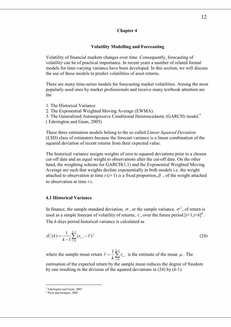
Chapter 4

Volatility Modelling and Forecasting

Volatility of financial markets changes over time. Consequently, forecasting of

volatility can be of practical importance. In recent years a number of related formal

models for time-varying variance have been developed. In this section, we will discuss

the use of these models to predict volatilities of asset returns.

There are many time-series models for forecasting market volatilities. Among the most

popularly used ones by market professionals and receive many textbook attention are

the

1. The Historical Variance

2. The Exponential Weighted Moving Average (EWMA).

3. The Generalized Autoregressive Conditional Heteroscedastic (GARCH) model.5

( Ederington and Guan, 2005)

These three estimation models belong to the so called Linear Squared Deviation

(LSD) class of estimators because the forecast variance is a linear combination of the

squared deviation of recent returns from their expected value.

The historical variance assigns weights of zero to squared deviations prior to a chosen

cut-off date and an equal weight to observations after the cut-off date. On the other

hand, the weighting scheme for GARCH(1,1) and the Exponential Weighted Moving

Average are such that weights decline exponentially in both models i.e. the weight

attached to observation at time t-(i+1) is a fixed proportion, β , of the weight attached

to observation at time t-i.

4.1 Historical Variance

In finance, the sample standard deviation, σ , or the sample variance, 2σ , of return is

used as a simple forecast of volatility of returns, tr , over the future period [t+1,t+h]6.

The k-days period historical variance is calculated as

1

2 2

0

1ˆ ( ) ( )

1

k

t t i

i

k r rk

σ−

−=

= −− ∑ (24)

where the sample mean return 1

0

1 k

t i

i

r rk

−

−=

= ∑ is the estimate of the mean µ . The

estimation of the expected return by the sample mean reduces the degree of freedom

by one resulting in the division of the squared deviations in (24) by (k-1).

5 Ederington and Guan, 2005 6 Poon and Granger, 2002

13

If the mean, µ , is known then the k-period historical variance is given by

1

2 2

0

1ˆ ( ) ( )

k

t t i

i

k rk

σ µ−

−=

= −∑ . (25)

An important issue that arises in the estimation of the historical variance is the noisy

estimate of the mean return. This is from the fact that the mean logarithmic return

depends on the range (length) of the return series in the sense that:

1 1(ln ln ) ln lnt t t t k k

r P P P Pr

k k k

− − +− −

= = =∑ ∑. (26)

Thus the mean return does not take into account the price movements or the number of

prices within the period. Most of the time, mean is set to zero to get a better forecast7.

Multiplying the variance by N, the number of trading days in a year and taking the

square root gives the annualised volatility

2ˆNσ σ= ⋅

⌢. (27)

Usually we take N=250. The value σ⌢ is the best estimator for the volatility from the

available price data and the volatility of any period of length, k, can be estimated from

this value.

The weighting scheme of the historical variance estimator is an assignment of zero

weight to the squared deviations before and at the time t-k while observations after

time t-n are assigned a weight of 1 k . A common convention is to set the length of the

period used in calculating the historical volatility, k, and that of the period of the

forecast, s, to be equal8. According to Figlewski (2004), a much longer period reduces

the forecasting errors.

4.2 The RiskMetrics’ Exponential Weighted Moving Average

The RiskMetrics’ Exponential Weighted Moving Average model (EWMA) will be

used to forecast the variances and covariances (volatilities and correlations) of the

multivariate normal distribution.

The RiskMetrics EWMA model uses historical observations to capture the dynamic

features of the volatility. It assigns the highest weight to the latest observations and the

least to the oldest observations in the volatility estimate. The assignment of these

weights enables volatility to react to large return (jump) in the market and following a

jump, the volatility declines exponentially as the weight of the jump falls.

The EWMA estimates the volatility for a given sequence of k returns as

7 Figlewski, 2004 8 Ederington and Guan, 2005

14

12

0

(1 ) ( )k

i

t i

i

r rσ λ λ−

−=

= − −∑ , (28)

where (0 1)λ λ< < is the decay factor. This parameter determines the relative weights

that are assigned to returns (observations) and the effective amount of data used in

estimating volatility. The latest return has weight (1 )λ− and the second latest

(1 )λ λ− and so on. The oldest return appears with weight 1(1 ) kλ λ −− .

We assume the sample mean r is zero and that infinite amounts of data are available.

Then by using the recursive feature of the exponential weighted moving average

(EWMA) estimator, the one -day variance forecast is

2 2 2

1, 1| 1, | 1 1,(1 )t t t t trσ λσ λ+ −= + − , (29)

where 2

1, 1|t tσ + denotes 1-day time 1t + forecast given information up to time t. Taking

the square root of both sides of (29) we get the one day volatility forecast as

2 2

1, 1| 1, | 1 1,(1 )t t t t trσ λσ λ+ −= + −. (30)

A simple proof of equations (29) and (30) are illustrated below.

2 2

1, 1| 1,

0

(1 ) i

t t t i

i

rσ λ λ∞

+ −=

= − ∑

( )2 2 2 2

1, 1, 1 1, 2(1 ) ...t t tr r rλ λ λ− −= − + + +

( )2 2 2 2

1, 1, 1 1, 2 1, 3(1 ) (1 )t t t tr r r rλ λ λ λ− − −= − + − + +

2 2

1, | 1 1,(1 )t t trλσ λ−= + −

and the volatility is obviously given by (30). For two return series, the EWMA

estimate of covariance for a given sequence of k returns is given by

1

1,2 1, 1 2, 2

0

(1 ) ( )( )k

i

k i k i

i

r r r rσ λ λ−

− −=

= − − −∑ . (31)

If we assume 1 2 0r r= = , then just as before it can be shown that

1

1,2 1, 2,

0

(1 )k

i

k i k i

i

r rσ λ λ−

− −=

= − ∑ (32)

Similar to the expression for the variance forecast equation (29), the covariance

forecast can be written in recursive form. The one-day covariance forecast between

any two return series, 1,tr and 2,tr made at time t is

15

2 2

12, 1| 12, | 1 1, 2,(1 ) .t t t t t tr rσ λσ λ+ −= + − . (33)

The corresponding one-day correlation forecast for the two returns is given by

2

12, 1|

12, 1|

1, 1| 2, 1|

t t

t t

t t t t

σρ

σ σ+

++ +

= . (34)

In managing risk, one may be interested in a longer horizon other than just one day

and hence we should construct an EWMA model over multiple horizon. The forecasts

of the variance and the covariance for k-period (i.e. over k-days) are respectively

2 2

1, | 1, 1|t k t t tkσ σ+ += or 1, | 1, 1|t k t t tkσ σ+ += (35)

and

12, |

2 2

12, 1|t k t t tkσ σ+ += 9

. (36)

The correlation forecast does not depend on the forecasting horizon. i.e.

2

12, 1|

12, | 12, 1|

1, 1| 2, 1|

t t

t k t t t

t t t t

σρ ρ

σ σ+

+ ++ +

= = (37)

It is observed that multiple day forecasts are simply multiples of one-day forecasts.

4.2.1 Estimating the Parameters of the RiskMetrics Model

The two estimation issues that arise in computation of estimates for the RiskMetrics

volatilities and covariances are the sample mean and the exponential decay factor λ .

In practice, the RiskMetrics model assumes zero mean for the sample. The largest

sample size available should be used to reduce the standard error. Choosing a suitable

decay factor is a necessity in forecasting volatility and correlations. One essential

issue is this estimation is the determination of an effective number of days (k) used in

forecasting. This is postulated in the RiskMetrics model to be determined by the

assumed tolerance level

(1 ) t

t k

α λ λ∞

=

= − ∑ . (38)

Expanding the summation we get

9 We illustrate simple Proof of Equations (35) and (36) in appendix A.3.

16

2(1 )[1 ...]kλ λ λ λ α− + + + = . (39)

Taken the natural logarithms of both sides, we find k as

ln

lnk

αλ

= . (40)

4.2.2 Determining the Decay Factor

The forecast of the variance of returns at time t+1, made one period earlier is defined

as 2 2

1 1|( )t t t tE r σ+ += where tE denotes the conditional expectation based on information

up to time t. Similarly for two return series, 1, 1tr + and 2, 1tr + , the forecast at time t+1 of

the covariance between the two return series made one period earlier is 2

1, 1 2, 1 12, 1|( )t t t t tE r r σ+ + += . In general, these results hold for any forecast made at

time , 1t j j+ ≥ .

The forecast error of the variance is defined as

2 2

1| 1 1|( ) ( )t t t t trε λ σ λ+ + += − (41)

with an expected value of zero. i.e.

2 2

1| 1 1|( ) ( ) 0t t t t t t tE E rε σ+ + += − = (42)

A natural consideration in choosing is to minimize average squared errors. We apply

this to daily forecasts of variance and according to RiskMetrics, an

appropriateλ should be chosen such that the root mean square (RMSE) of the errors

12 2 2

1 1|

0

1ˆ[ ( )]

k

v t i t i t i

i

RMSE rk

σ λ−

− + − + −=

= −∑ (43)

is minimized.

Similarly, the RMSE expression for the covariance forecast can be derived. The

covariance forecast error is

2

12, 1| 1, 1 2, 1 12, 1|t t t t t tr rε σ+ + + += − (44)

and its conditional expected value is

2

12, 1| 1, 1 2, 1 12, 1|( ) ( ) 0t t t t t t t tE E r rε σ+ + + += − = . (45)

The RMSE of the covariance forecast is given by

17

12 2

1, 1 2, 1 12, 1|

0

1ˆ[ ( )]

k

c t i t i t i t

i

RMSE r rk

σ λ−

− + − + − +=

= −∑ . (46)

In principle, we can find a set of optimal decay factors, one for each covariance can be

determined such that the estimated covariance matrix is symmetric and positive

definite. RiskMetrics present a method for choosing one optimal decay factor to be

used in estimation of the entire covariance matrix. They found 0.94λ = to be the

optimal for one-day forecast and 0.97λ = for one month (25 trading days) forecast.10

4.3 The Generalized Autoregressive Conditional

Heteroscedastic (GARCH) model

Generalized ARCH, or GARCH, framework developed by Bollerslev (1986) explains

variance by two distributed lags, one on past squared residuals to capture high

frequency effects, and the second on lagged values of the variance itself, to capture

longer term influences. These enable volatility clustering to be captured and the

leptokurtosis nature of the unconditional distribution of returns although it is a simple

model.

Let tψ be the information set (σ -field) of all information through time t. A

stochastic process { }tX is a GARCH(p, q) if

1( | )=0t tE X ψ − (47)

and

1( | )=t t tVar X hψ − (48)

with

2

0

1

q p

t i t i j t j

i j

h X hα α β− −=

= + +∑ ∑ (49)

where 00, 0, 0q p α> ≥ > and 0iα > for i=1,…,q, 0, 1,...,j j pβ > = . These

conditions are needed to guarantee that the conditional variance 0th > . It is usually

also assumed that t/tX h is i.i.d with mean 0 and variance 1 (“strong GARCH”).

The simplest and the most commonly used GARCH process is the GARCH(1,1)

process for which

10 RiskMetrics, 1996

18

2

0 1 1 1 1t t th X hα α β− −= + + (50)

where 0 10, 0α α> ≥ and 1 0β > .

The intuitive forecasting strategy of the GARCH (1,1) model is that the estimated

volatility at a given date is a combination of the long run variance and the variance

expected for last period, adjusted to incorporate the size of the last period's observed

shock11.

Every GARCH (p, q) is defined recursively and as earlier stated conditions are needed

to guarantee the existence of stationary solutions. We take a look at such condition for

the GARCH(1,1) process. We divide (47) by the square root of the conditional

variance of tX and obtain:

1| , 1, 2,...,tt

t

Xt T

hψ − = (51)

Then tZ defined as , 1, 2,...,tt

t

XZ t T

h= = , should be independent and identically

distributed. Suppose that the process is stationary. Then

2

1 1( ) ( ) ( )t t tE X E h E h h− −= = = (52)

In order to find the unconditional variance, we take the unconditional expectation of

both sides of equation (50). Solving for h we find

0

1 11h

αα β

=− −

. (53)

It can be shown that that if 1 1 1α β+ < and (0,1)tZ N∼ then tX is (weakly) stationary.

The sum, 1 1α β+ , is called the persistence parameter. A persistence value that is close

to one is describe as high and it implies a shock in the return series will decay slowly.

A low persistence on the other hand leads to a fast decay of the shock to its long run

variance.12

4.3.1 Estimation of the GARCH(1,1) Model

In this section we consider maximum likelihood estimation of the parameters of the

GARCH(1,1) as indicated in Bollerslev, 1986. The joint density of the observations

, 1, 2,...,t

X t T= can be written as the product of the conditional densities conditioning

on the previous observations:

1 2 1 2 1 1, ,..., 1 2 | , ,..., 1 2 1 1

2

( , ,..., ) ( | , ,..., ) ( )T j j

T

X X X T X X X X j j x

j

F x x x f x x x x f x− −

=

= ∏ . (54)

11 Figlewski, 2004 12 Jorion, 1997

19

The marginal density of 1X is dropped for simplicity. With the conditional normal

assumption, the conditional density of , 2,...,kX k T= , conditioning on 1 1,..., kX X − is

given by

1 2 1

2

| , ,..., 1, 2 1

1( | ,..., ) exp

22k k

kX X X X k k

kk

xf x x x x

hhπ− −

= −

(55)

and the conditional likelihood function, given 1X and 1h is:

2 1 10 1 1 ,..., | , 2 1 1( , , ) ( ,..., | , )kX X X h kL f x x x hα α β =

2

**2

1exp

22

Tk

j jj

x

hhπ=

= −

∏ (56)

Where * 2 *

0 1 1 1 1j t jh X hα α β− −= + + are obtained recursively. Substituting 1h by its

expected value 1 0 1 1( ) 1E h α α β= − − we find the log likelihood function as

* 2 *

0 1 1

2

1( , , | , ) log

2

T

j j j

j

l X h h x hα α β=

= − +

∑ (57)

where 1( ,..., )TX X X ′= and 1( ,..., )Th h h ′= 13 .

4.3.2 The GARCH(1,1) k-period Volatility Forecast

The k-day volatility forecast can also be found by using the GARCH model. Suppose

the model is estimated using daily returns on a stock. Similar to equation (13),

multiple-day returns are constructed from one day returns by summing across time

, 1 ...t t k t t Tr r r r+ += + + + . (58)

Under the condition that returns are uncorrelated across days, the multiple-day

variance as of 1t − is given by

2 2 2 2

, 1 1 1 1 1| ( | ) ( | ) ... ( | )t t k t t t t t T tE r E r E r E rψ ψ ψ ψ+ − − + − − = + + + . (59)

The forecast of the variance k-period ahead is derived as follows: Let 1 10,s q α β> = +

and 1tψ − -information at time t. Then

13 Bollerslev (1986)

20

2 2

0 1 1 -1 1( 1)t s t s t s t sh qX h Zα α+ + − + + −= + + −

2

0 -1 1 -1 1( 1)t s t s t sqh h Zα α+ + + −= + + − . (60)

1( | ) 1t s tE Z ψ+ − = (61)

so

0 -1( | ) ( | )t s t t s tE h qE hψ α ψ+ += + . (62)

Therefore

0 -1( | ) ( | )t k t t k tE h qE hψ α ψ+ += +

( )0 0 -2

2

0 0 -2

( | )

( | )

t k t

t k t

q qE h

q q E h

α α ψ

α α ψ+

+

= + +

= + +

.

.

.

2 1

0 0 0 +1... (h | )k k

t tq q q Eα α α ψ− −= + + + +

0

1

0 0 0

1

1

... ( | )

kt

k k

t t

hq

q

q q q E h

α

α α α ψ−

−−

= + + + +��

1 10 1 1

1 1

1 ( )( ) .

1 ( )

kk

thα β

α α βα β

− += + +

− + (63)

Note that if 1 1 1α β+ < , then

0

1 1

lim ( | )1

t k tk

E hα

ψα β+→∞

=− −

(64)

The volatility forecast over the future period from 1t + to t k+ denoted by ,G tσ , is an

average of the expected volatility on each day from t to t k+ i.e.

,

1

1( | )

k

G t t k t

i

E hk

σ ψ+=

= ∑ (65)

where the expected values are given by (63).

4.4 Measuring Forecasting Performance

The In-Sample and Out-of-Sample forecasting ability of the various volatility models

21

will be measured by the Root Mean Squared Forecasting Errors (RMFSE). In the In-

Sample comparison of the various forecasting models, the entire data sets for each

return series will be used. To compare the out-of-sample forecasting performance of

the variuous volatility model, we will split the sample into two parts. The first, which

is used to estimate the parameters of the GARCH(1,1) model contains at least two

thirds of the entire sample. The remaining part of the sample will be used to test the

forecasting ability of the volatility models. The parameters of the GARCH(1,1)

model will be estimated each time with a rolling constant sample size. Thus for a

forecasting horizon of x, at each forecasting date we add x amount of new data and

subtract x amount of the oldest data.

The realised volatility at each forecast date is calculated from the expression

2

,

1

1 N

R t t i

i

rN

σ +=

= ∑ . (66)

Let 2

,F tσ be the forecast of the variance given by one of the volatility models, then the

RMSFE for a model is given by equation

2

, ,

1( )F t R t

t s

RMSFEn

σ σ∈

= −∑ . (67)

n and s denotes the number of forecasts and the set of times at which ex ante forecasts

are produced respectively in the above expression14.

14 Xu and Taylor (1995)

22

Chapter 5

Data Analysis

In this section we evaluate the performance of the three models on different financial

time series taking from various stocks. The dataset that we discuss here are DJ-AIG

Commodity Index, S&P500 index, DJ-Industrial Average, OMXS30 Index, Ghanaian

Cedi and the US dollar exchange rate i.e. CEDI/USD and the Yield on the US 3

Months Treasury Bill. We first describe the dataset above and the historical variance

in section 5.1. Then, we fit the GARCH(1,1) model and the RiskMetrics EWMA

model to the datasets in section 5.2 and section 5.3 respectively. Lastly, in section 5.4,

we compare the various forecasting models and make our conclusions in section 5.5.

5.1 Description of Data

The S&P500 consist of weighted market value of 500 of the most widely held stocks

in the US stock market. This is considered as a more representative index with

coverage of over 70% of the US equity market. The S&P500 dataset has a total of

3828 observations from September 19, 1991 to November 22, 2006.

The DJ-AIG Commodity Index (DJ-AIGCI) is a rolling index composed of 19

physical commodities’ future contracts traded on the US stock exchanges. According

to Investopedia, the primary goal of the DJ-AIGCI is to provide a diversified

commodities index with weightings based on the economic significance of individual

components, while maintaining low volatility and sufficient liquidity. The DJ-AIGCI

data is from January 2, 1991 to January 31, 2006 with 3771 observations.

The Dow Jones Industrial Index Average (DJIA) comprises of stocks of 30 leading

industrial companies in the US. The index is the most widely quoted US stock index

and the oldest despite its small number of companies. The DJIA dataset being

considered is the historical price data between September 4, 1990 to November 22,

2006 with a total of 4092 observations.

The OMXS30 was introduced by the Swedish exchange for options and forwards. It

is a market value weighted index of 30 leading stocks on the OMX Stock Exchange

in Stockholm and accounts for about 70% of trading conducted on the exchange. Data

is from January 3, 2000 to November 20, 2006 and comprises of 1721 observations.

CEDI/USD foreign exchange rate from April 23, 1994 to November 5, 2006 with

total observations of 4613 and finally, the yield on 3 months US Treasury bills from

August 23, 1989 to August 22, 2000 with 2612 observations are considered.

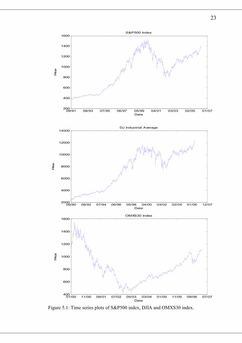
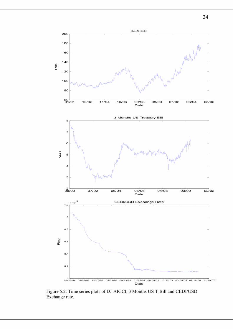
The time series plot of the S&P500, DJIA and OMXS30 are shown in figure 5.1

whilst that of DJ-AIGCI, 3 months US Treasury bill yield and CEDI/USD exchange

rate are shown in figure 5.2. All of the plots exhibit clustering of small or large

movements in price, a feature of volatility process of assets prices. Engle and Patton

(2000) states that, this feature was reported in the earlier works by Mandelbort

23

09/91 08/93 07/95 06/97 05/99 04/01 03/03 02/05 01/07200

400

600

800

1000

1200

1400

1600S&P500 Index

Date

Price

09/90 08/92 07/94 06/96 05/98 04/00 03/02 02/04 01/06 12/072000

4000

6000

8000

10000

12000

14000

Date

Price

DJ Industrial Average

01/00 11/00 09/01 07/02 05/03 03/04 01/05 11/05 09/06 07/07400

600

800

1000

1200

1400

1600OMXS30 Index

Date

Price

Figure 5.1: Time series plots of S&P500 index, DJIA and OMXS30 index.

24

01/91 12/92 11/94 10/96 09/98 08/00 07/02 06/04 05/0660

80

100

120

140

160

180

200

Date

Price

DJ-AIGCI

08/90 07/92 06/94 05/96 04/98 03/00 02/022

3

4

5

6

7

83 Months US Treasury Bill

Date

Yield

03/23/94 08/05/95 12/17/96 05/01/98 09/13/99 01/25/01 06/09/02 10/22/03 03/05/05 07/18/06 11/30/070

0.2

0.4

0.6

0.8

1

1.2x 10

-3 CEDI/USD Exchange Rate

Date

Rate

Figure 5.2: Time series plots of DJ-AIGCI, 3 Months US T-Bill and CEDI/USD

Exchange rate.

25

(1963), Fama (1965) and numerous other studies such as Chou (1988), Schwert

(1989) and Baillie et al (1996). We base the volatility dynamics on each series’

exclusive history but Engle and Patton (2000) reports that, financial assets prices are

affected by the market around it as well as deterministic events such as company

announcements and macroeconomics announcements.

This is evident in the plot of the CEDI/USD exchange rate. In 1992, Ghana made a

transition from military rule to constitutional rule. The military junta at the time

transformed itself into a political party and subsequently won the election. Many

businesses did not have much confidence in the economy and thus the local currency,

the cedi, continued to depreciate against all the other major trading currencies. In

2000, the opposition won the elections and brought about good fiscal policies. One of

the significant one was the removal of government subsidies from petroleum products

which was the major determining factor in the strength of the cedi. Hence the

Ghanaian Cedi’s fall against the US dollar in the 2000’s has been stable as compared

to the 1990’s.

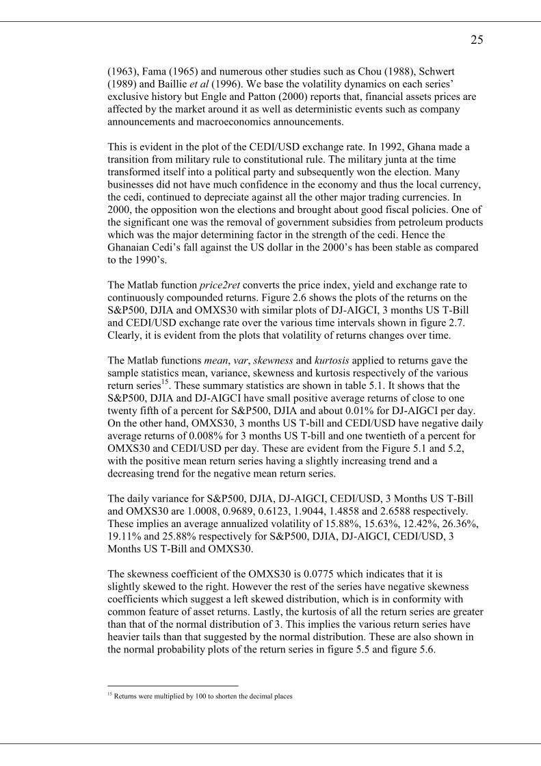
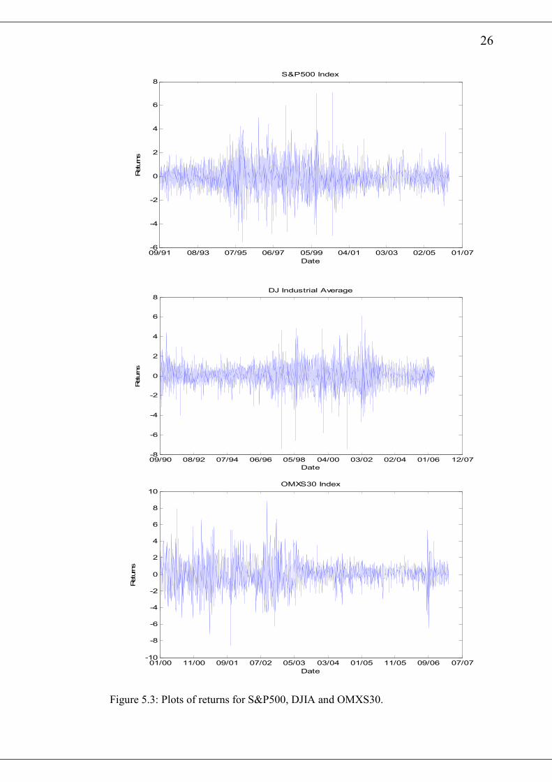
The Matlab function price2ret converts the price index, yield and exchange rate to

continuously compounded returns. Figure 2.6 shows the plots of the returns on the

S&P500, DJIA and OMXS30 with similar plots of DJ-AIGCI, 3 months US T-Bill

and CEDI/USD exchange rate over the various time intervals shown in figure 2.7.

Clearly, it is evident from the plots that volatility of returns changes over time.

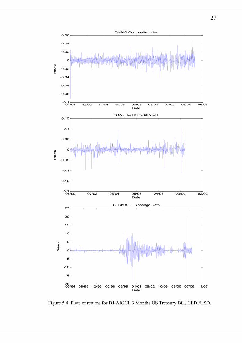
The Matlab functions mean, var, skewness and kurtosis applied to returns gave the

sample statistics mean, variance, skewness and kurtosis respectively of the various

return series15. These summary statistics are shown in table 5.1. It shows that the

S&P500, DJIA and DJ-AIGCI have small positive average returns of close to one

twenty fifth of a percent for S&P500, DJIA and about 0.01% for DJ-AIGCI per day.

On the other hand, OMXS30, 3 months US T-bill and CEDI/USD have negative daily

average returns of 0.008% for 3 months US T-bill and one twentieth of a percent for

OMXS30 and CEDI/USD per day. These are evident from the Figure 5.1 and 5.2,

with the positive mean return series having a slightly increasing trend and a

decreasing trend for the negative mean return series.

The daily variance for S&P500, DJIA, DJ-AIGCI, CEDI/USD, 3 Months US T-Bill

and OMXS30 are 1.0008, 0.9689, 0.6123, 1.9044, 1.4858 and 2.6588 respectively.

These implies an average annualized volatility of 15.88%, 15.63%, 12.42%, 26.36%,

19.11% and 25.88% respectively for S&P500, DJIA, DJ-AIGCI, CEDI/USD, 3

Months US T-Bill and OMXS30.

The skewness coefficient of the OMXS30 is 0.0775 which indicates that it is

slightly skewed to the right. However the rest of the series have negative skewness

coefficients which suggest a left skewed distribution, which is in conformity with

common feature of asset returns. Lastly, the kurtosis of all the return series are greater

than that of the normal distribution of 3. This implies the various return series have

heavier tails than that suggested by the normal distribution. These are also shown in

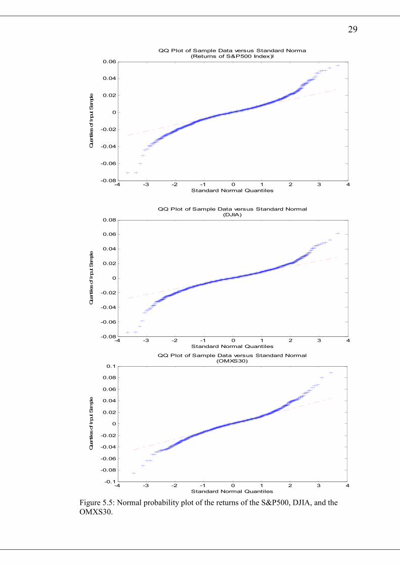
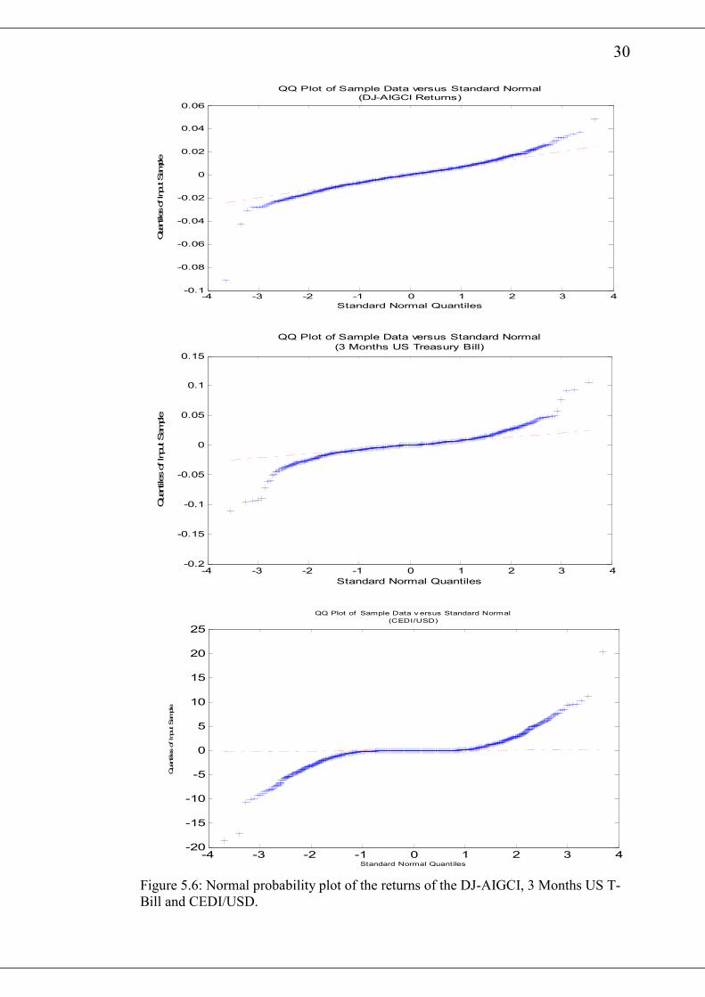
the normal probability plots of the return series in figure 5.5 and figure 5.6.

15 Returns were multiplied by 100 to shorten the decimal places

26

09/91 08/93 07/95 06/97 05/99 04/01 03/03 02/05 01/07-6

-4

-2

0

2

4

6

8

Date

Returns

S&P500 Index

09/90 08/92 07/94 06/96 05/98 04/00 03/02 02/04 01/06 12/07-8

-6

-4

-2

0

2

4

6

8DJ Industrial Average

Date

Returns

01/00 11/00 09/01 07/02 05/03 03/04 01/05 11/05 09/06 07/07-10

-8

-6

-4

-2

0

2

4

6

8

10OMXS30 Index

Date

Returns

Figure 5.3: Plots of returns for S&P500, DJIA and OMXS30.

27

01/91 12/92 11/94 10/96 09/98 08/00 07/02 06/04 05/06-0.1

-0.08

-0.06

-0.04

-0.02

0

0.02

0.04

0.06DJ-AIG Composite Index

Date

Returns

08/90 07/92 06/94 05/96 04/98 03/00 02/02-0.2

-0.15

-0.1

-0.05

0

0.05

0.1

0.153 Months US T-Bill Yield

Date

Returns

03/94 08/95 12/96 05/98 09/99 01/01 06/02 10/03 03/05 07/06 11/07-20

-15

-10

-5

0

5

10

15

20

25CEDI/USD Exchange Rate

Date

Returns

Figure 5.4: Plots of returns for DJ-AIGCI, 3 Months US Treasury Bill, CEDI/USD.

28

Estimates S&P500 DJIA DJ-

AIGCI

CEDI/USD US 3

Months

T-Bill

OMXS30

Mean 0.0336 0.0379 0.0146 -0.0486 -0.0084 -0.0053

Variance 1.0008 0.9689 0.6123 1.9044

1.4858

2.6588

Skewness -0.1161 -0.2134 -0.3019

-0.3021

-0.2382 0.0775

Kurtosis 7.1872 7.8196

9.6007

39.6932 18.0065 5.6187

Table 5.1: summary statistics of the returns.

All the figures show deviations from normality by its deviation from the straight

line16.

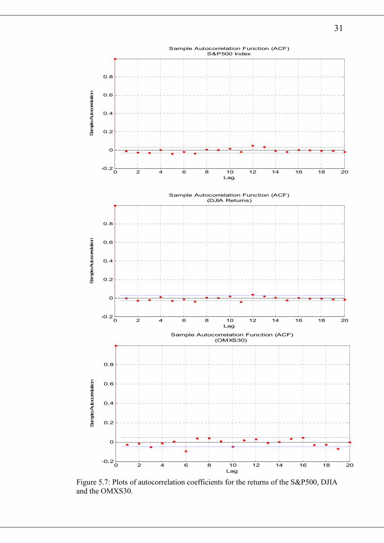
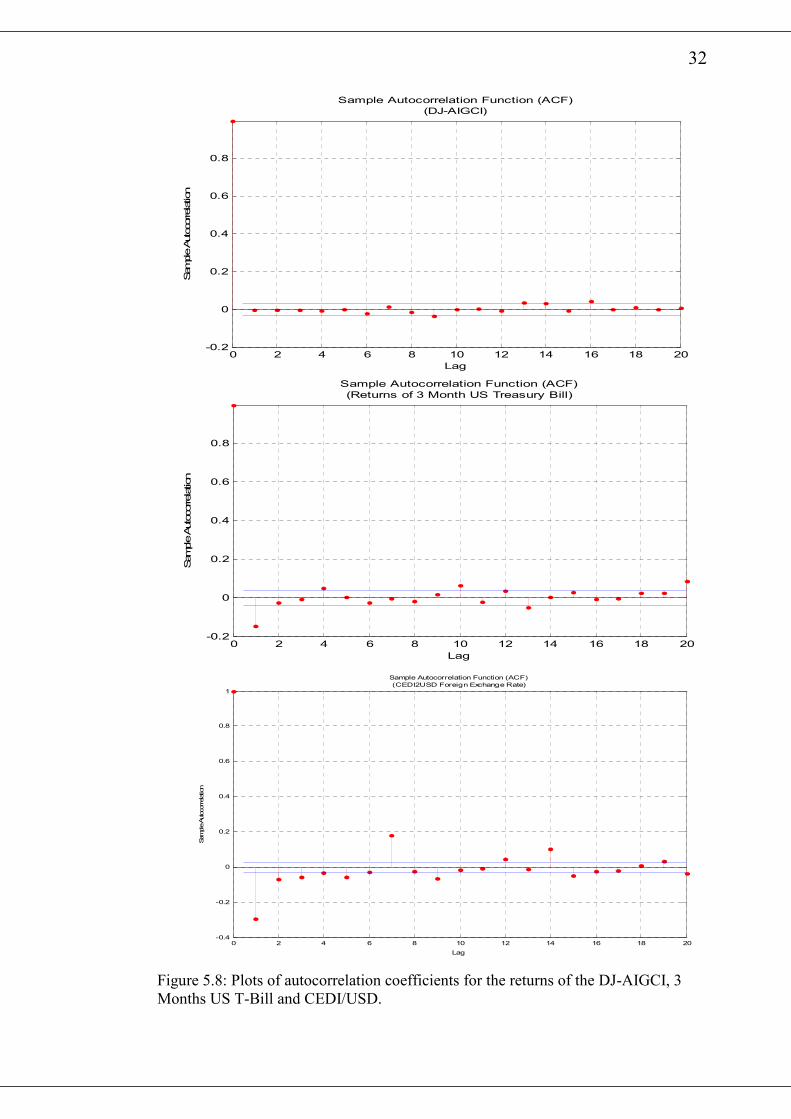
The Matlab function autocorr gives the autocorrelation plots of the various return

series and are presented in figures 5.7 and 5.8. With the exception of the CEDI/USD,

all the other returns show very weak serial dependence since almost all the

autocorrelation coefficients lay within the 95% approximate confidence limits.

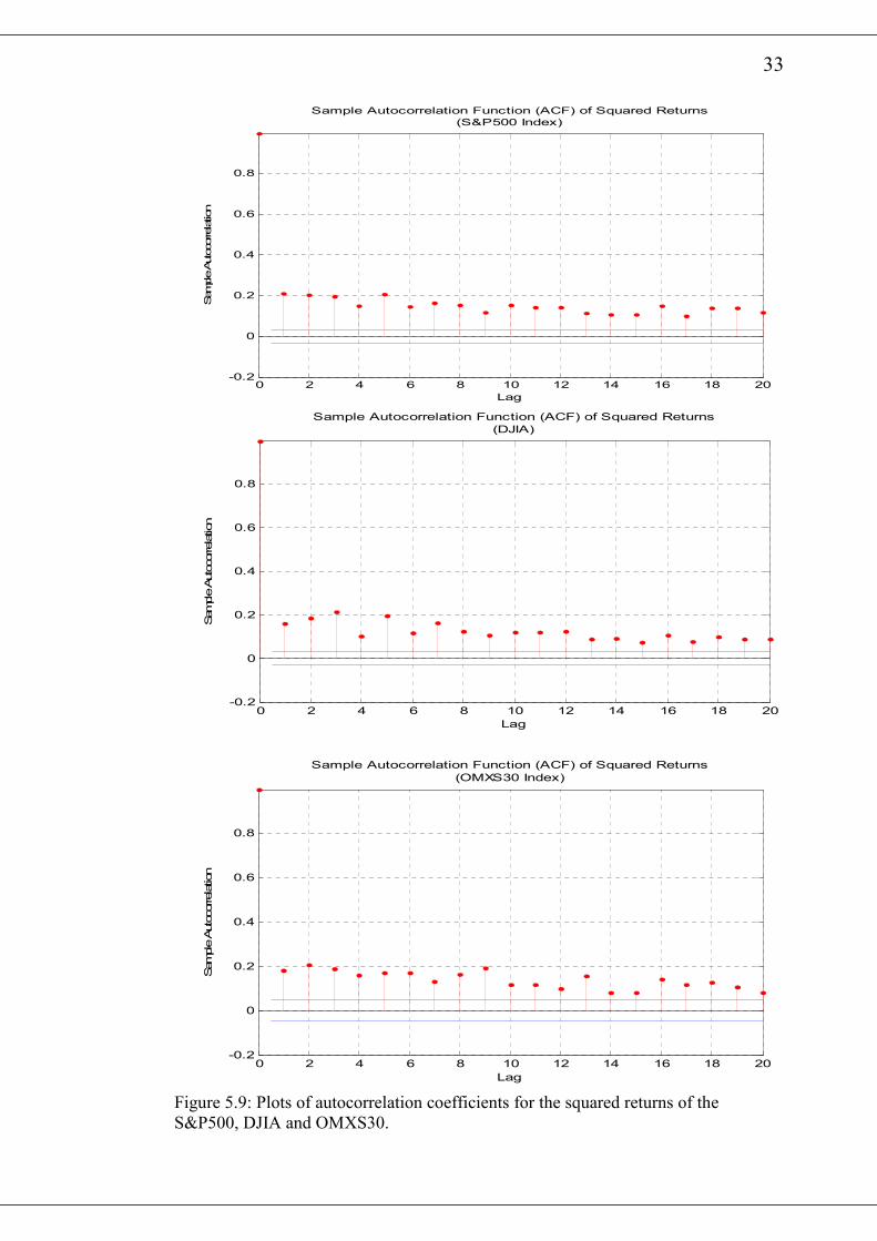
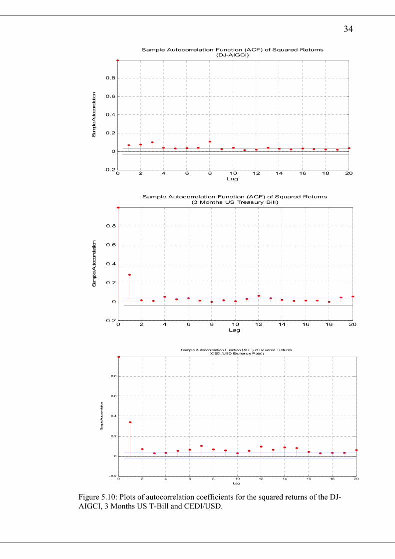
However, an inspection of the autocorrelation plots of squared returns in figure 5.9

and figure 5.10 indicates that most of the autocorrelation coefficients are above the

95% confidence limits. This means that there are considerable serial dependence in

the return series17.

The Ljung-Box Q-statistics for the returns and squared returns of the various series

are presented in table 5.2 and table 5.3 respectively. The tests show that, raw returns

for S&P500 and DJ-AIGCI have no significant autocorrelation up to the 20th lag.

Raw returns for DJIA, 3M-US-T-Bill and OMXS30 however have some weak

autocorrelation in it. However CEDI/USD raw returns show very significant

autocorrelation. A look at the Ljung-Box Q test for squared returns shows strong

evidence of autocorrelations among squared returns for each series. A property of

financial time series reported in the earlier works of Miller (1979).

5.2 Fitting the GARCH(1,1) Model.

In this section, we estimate the parameters 0α , 1α and 1β of the GARCH(1,1) model

and the in-sample estimates of the volatility. The Matlab command garchfit, models

the return series as GARCH(1,1) and estimates the parameters 0α , 1α and 1β via

maximum likelihood. The estimates of the parameters of the various series are shown

in table 5.4. The return series, CEDI/USD, has the highest persistence value which is

16 See Appendix A.1.2 for description of the normal probability plot 17 These buttress earlier works of several people including Miller (1979) and also in RiskMetrics (1996).

29

-4 -3 -2 -1 0 1 2 3 4-0.08

-0.06

-0.04

-0.02

0

0.02

0.04

0.06

Standard Normal Quantiles

Quantiles of Input Sample

QQ Plot of Sample Data versus Standard Norma

(Returns of S&P500 Index)l

-4 -3 -2 -1 0 1 2 3 4-0.08

-0.06

-0.04

-0.02

0

0.02

0.04

0.06

0.08



QQ Plot of Sample Data versus Standard Normal

(DJIA)

-4 -3 -2 -1 0 1 2 3 4-0.1

-0.08

-0.06

-0.04

-0.02

0

0.02

0.04

0.06

0.08

0.1




(OMXS30)

Figure 5.5: Normal probability plot of the returns of the S&P500, DJIA, and the

OMXS30.

30

-4 -3 -2 -1 0 1 2 3 4-0.1

-0.08

-0.06

-0.04

-0.02

0

0.02

0.04

0.06




(DJ-AIGCI Returns)

-4 -3 -2 -1 0 1 2 3 4-0.2

-0.15

-0.1

-0.05

0

0.05

0.1

0.15




(3 Months US Treasury Bill)

-4 -3 -2 -1 0 1 2 3 4-20

-15

-10

-5

0

5

10

15

20

25



QQ Plot of Sample Data v ersus Standard Normal

(CEDI/USD)

Figure 5.6: Normal probability plot of the returns of the DJ-AIGCI, 3 Months US T-

Bill and CEDI/USD.

31

0 2 4 6 8 10 12 14 16 18 20-0.2

0

0.2

0.4

0.6

0.8

Lag



S&P500 Index

0 2 4 6 8 10 12 14 16 18 20-0.2

0

0.2

0.4

0.6

0.8

Lag



(DJIA Returns)

0 2 4 6 8 10 12 14 16 18 20-0.2

0

0.2

0.4

0.6

0.8

Lag



(OMXS30)

Figure 5.7: Plots of autocorrelation coefficients for the returns of the S&P500, DJIA

and the OMXS30.

32

0 2 4 6 8 10 12 14 16 18 20-0.2

0

0.2

0.4

0.6

0.8

Lag



(DJ-AIGCI)

0 2 4 6 8 10 12 14 16 18 20-0.2

0

0.2

0.4

0.6

0.8

Lag



(Returns of 3 Month US Treasury Bill)

0 2 4 6 8 10 12 14 16 18 20-0.4

-0.2

0

0.2

0.4

0.6

0.8

1

Lag



(CEDI2USD Foreign Exchange Rate)

Figure 5.8: Plots of autocorrelation coefficients for the returns of the DJ-AIGCI, 3

Months US T-Bill and CEDI/USD.

33

0 2 4 6 8 10 12 14 16 18 20-0.2

0

0.2

0.4

0.6

0.8

Lag


Sample Autocorrelation Function (ACF) of Squared Returns

(S&P500 Index)

0 2 4 6 8 10 12 14 16 18 20-0.2

0

0.2

0.4

0.6

0.8

Lag



(DJIA)

0 2 4 6 8 10 12 14 16 18 20-0.2

0

0.2

0.4

0.6

0.8

Lag



(OMXS30 Index)

Figure 5.9: Plots of autocorrelation coefficients for the squared returns of the

S&P500, DJIA and OMXS30.

34

0 2 4 6 8 10 12 14 16 18 20-0.2

0

0.2

0.4

0.6

0.8

Lag



(DJ-AIGCI)

0 2 4 6 8 10 12 14 16 18 20-0.2

0

0.2

0.4

0.6

0.8

Lag



(3 Months US Treasury Bill)

0 2 4 6 8 10 12 14 16 18 20-0.2

0

0.2

0.4

0.6

0.8

Lag



(CEDI/USD Exchange Rate))

Figure 5.10: Plots of autocorrelation coefficients for the squared returns of the DJ-

AIGCI, 3 Months US T-Bill and CEDI/USD.

35

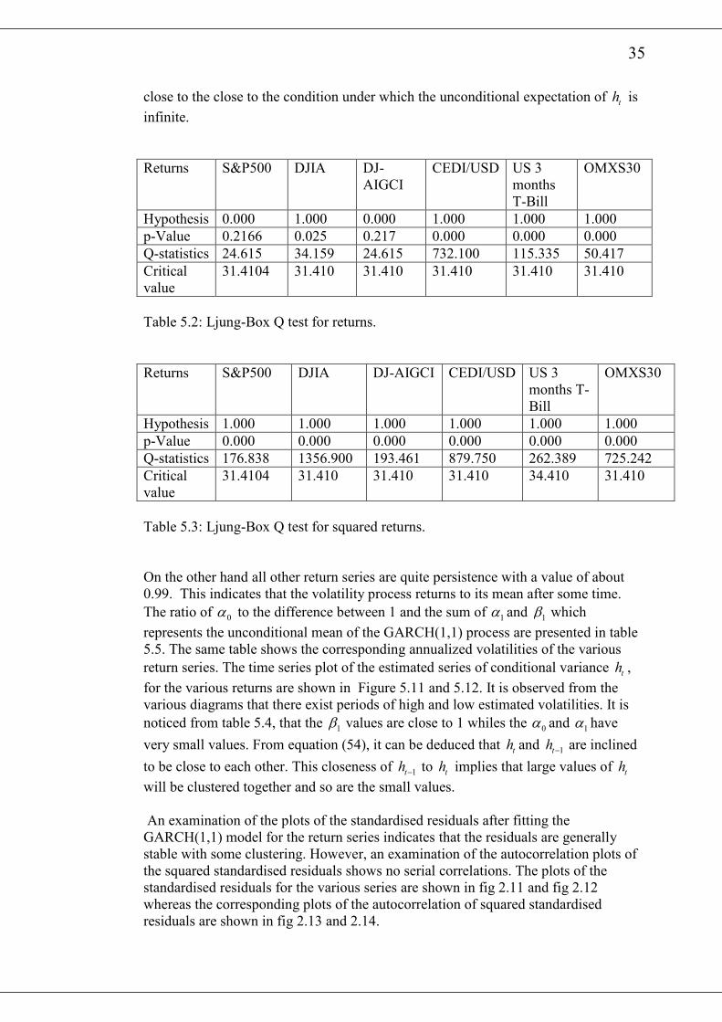
close to the close to the condition under which the unconditional expectation of th is

infinite.

Returns S&P500 DJIA DJ-

AIGCI

CEDI/USD US 3

months

T-Bill

OMXS30

Hypothesis 0.000 1.000 0.000 1.000 1.000 1.000

p-Value 0.2166 0.025 0.217 0.000 0.000 0.000

Q-statistics 24.615 34.159 24.615 732.100 115.335 50.417

Critical

value

31.4104 31.410 31.410 31.410 31.410 31.410

Table 5.2: Ljung-Box Q test for returns.

Returns S&P500 DJIA DJ-AIGCI CEDI/USD US 3

months T-

Bill

OMXS30

Hypothesis 1.000 1.000 1.000 1.000 1.000 1.000

p-Value 0.000 0.000 0.000 0.000 0.000 0.000

Q-statistics 176.838 1356.900 193.461 879.750 262.389 725.242

Critical

value

31.4104 31.410 31.410 31.410 34.410 31.410

Table 5.3: Ljung-Box Q test for squared returns.

On the other hand all other return series are quite persistence with a value of about

0.99. This indicates that the volatility process returns to its mean after some time.

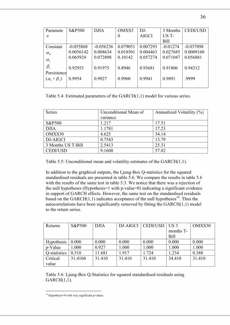
The ratio of 0α to the difference between 1 and the sum of 1α and 1β which

represents the unconditional mean of the GARCH(1,1) process are presented in table

5.5. The same table shows the corresponding annualized volatilities of the various

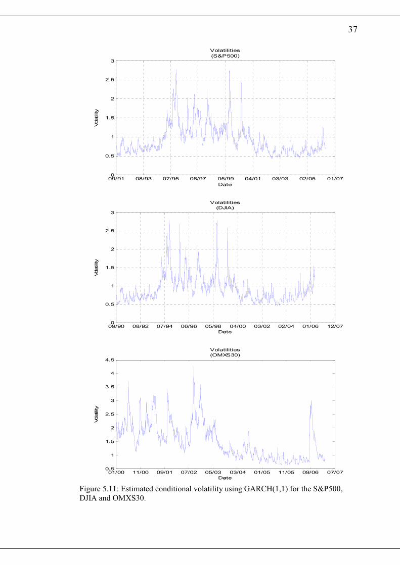
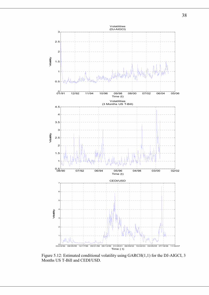
return series. The time series plot of the estimated series of conditional variance th ,

for the various returns are shown in Figure 5.11 and 5.12. It is observed from the

various diagrams that there exist periods of high and low estimated volatilities. It is

noticed from table 5.4, that the 1β values are close to 1 whiles the 0α and 1α have

very small values. From equation (54), it can be deduced that th and 1th − are inclined

to be close to each other. This closeness of 1th − to th implies that large values of th

will be clustered together and so are the small values.

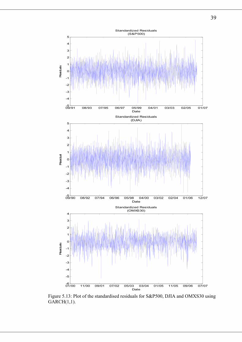
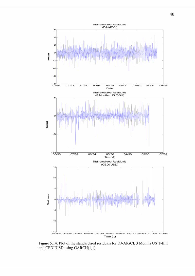
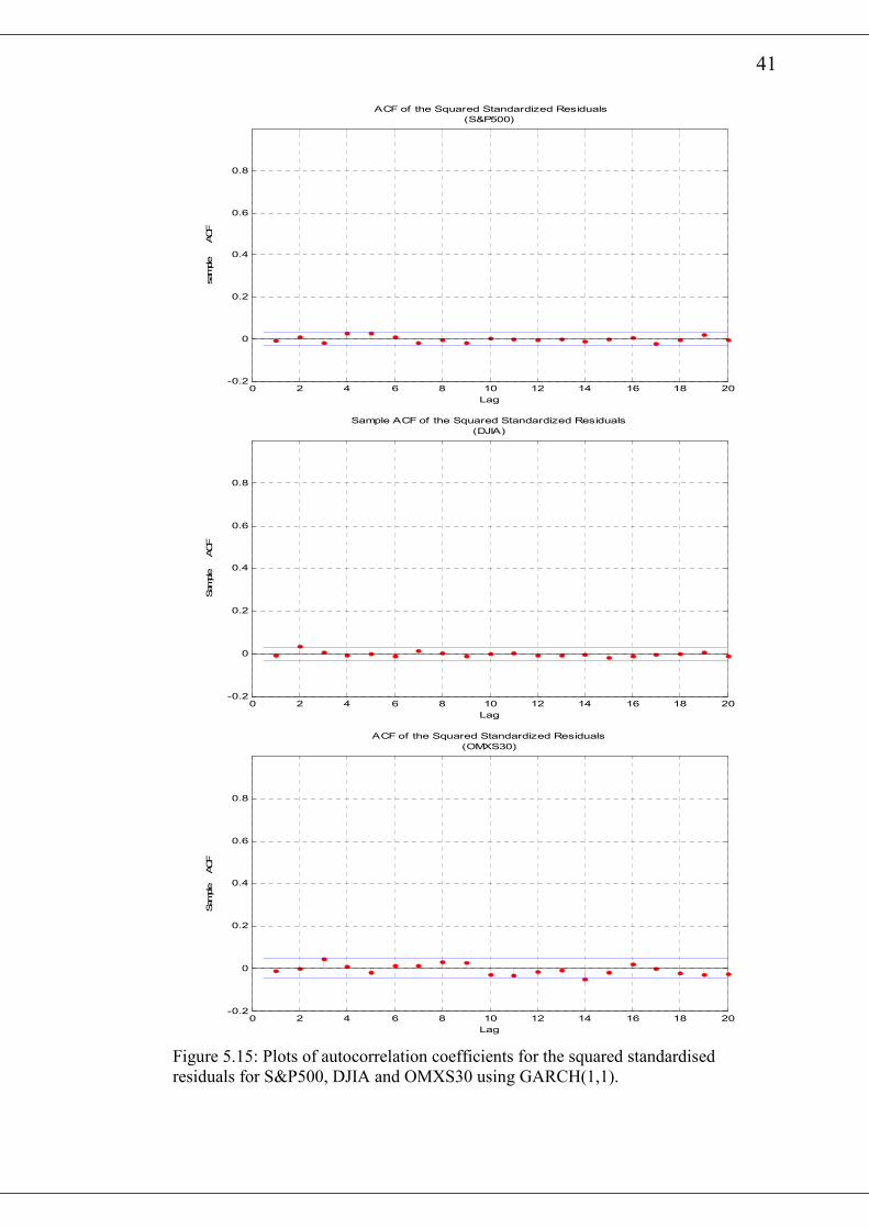
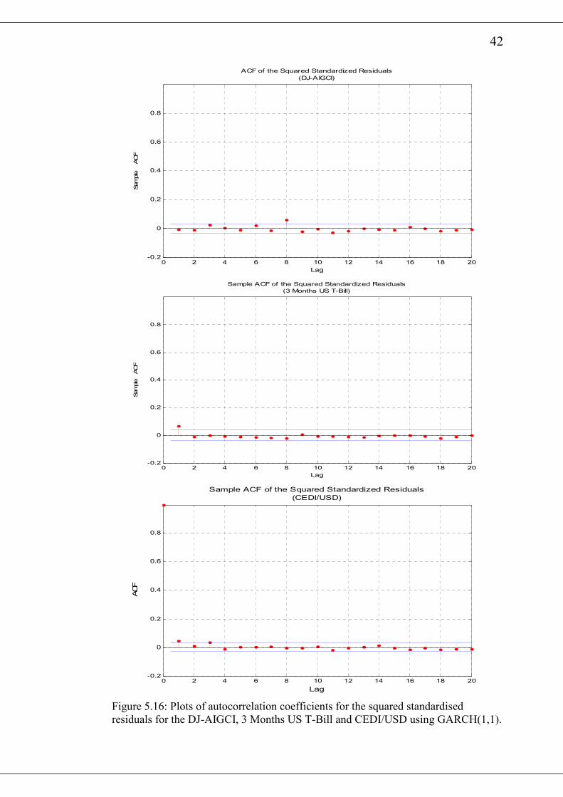
An examination of the plots of the standardised residuals after fitting the

GARCH(1,1) model for the return series indicates that the residuals are generally

stable with some clustering. However, an examination of the autocorrelation plots of

the squared standardised residuals shows no serial correlations. The plots of the

standardised residuals for the various series are shown in fig 2.11 and fig 2.12

whereas the corresponding plots of the autocorrelation of squared standardised

residuals are shown in fig 2.13 and 2.14.

36

Paramete

-r

S&P500 DJIA OMXS3

0

DJ-

AIGCI

3 Months

US T-

Bill

CEDI/USD

Constant

0α

1α

1β

Persistence

( 1α + 1β )

-0.055868

0.0056142

0.065924

0.92953

0.9954

-0.056236

0.008634

0.072898

0.91975

0.9927

0.079051

0.018501

0.10142

0.8946

0.9960

0.007293

0.004463

0.057274

0.93681

0.9941

-0.01274

0.027685

0.071047

0.91806

0.9891

-0.037098

0.0009160

0.056881

0.94312

.9999

Table 5.4: Estimated parameters of the GARCH(1,1) model for various series.

Series Unconditional Mean of

variance

Annualized Volatility (%)

S&P500 1.217 17.51

DJIA 1.1781 17.23

OMXS30 4.625 34.14

DJ-AIGCI 0.7543 13.79

3 Months US T-Bill 2.5413 25.31

CEDI/USD 9.1600 57.82

Table 5.5: Unconditional mean and volatility estimates of the GARCH(1,1).

In addition to the graphical outputs, the Ljung-Box Q-statistics for the squared

standardised residuals are presented in table 5.6. We compare the results in table 5.6

with the results of the same test in table 5.3. We notice that there was a rejection of

the null hypotheses (Hypothesis=1 with p-value=0) indicating a significant evidence

in support of GARCH effects. However, the same test on the standardised residuals

based on the GARCH(1,1) indicates acceptance of the null hypotheses18. Thus the

autocorrelations have been significantly removed by fitting the GARCH(1,1) model

to the return series.


months T-

Bill

OMXS30

Hypothesis 0.000 0.000 0.000 0.000 0.000 0.000

p-Value 1.000 0.927 1.000 1.000 1.000 1.000

Q-statistics 0.510 11.681 1.917 1.724 1.234 0.388

Critical

value

31.4104 31.410 31.410 31.410 34.410 31.410

Table 5.6: Ljung-Box Q-Statistics for squared standardised residuals using

GARCH(1,1).

18 Hypothesis=0 with very significant p-values

37

09/91 08/93 07/95 06/97 05/99 04/01 03/03 02/05 01/070

0.5

1

1.5

2

2.5

3

Volatilities

(S&P500)

Volatility

Date

09/90 08/92 07/94 06/96 05/98 04/00 03/02 02/04 01/06 12/070

0.5

1

1.5

2

2.5

3

Volatilities

(DJIA)

Volatility

Date

01/00 11/00 09/01 07/02 05/03 03/04 01/05 11/05 09/06 07/070.5

1

1.5

2

2.5

3

3.5

4

4.5

Volatilities

(OMXS30)

Date

Volatility

Figure 5.11: Estimated conditional volatility using GARCH(1,1) for the S&P500,

DJIA and OMXS30.

38

01/91 12/92 11/94 10/96 09/98 08/00 07/02 06/04 05/060

0.5

1

1.5

2

2.5

3

Volatilities

(DJ-AIGCI)

Volatility

Time (t)

08/90 07/92 06/94 05/96 04/98 03/00 02/020.5

1

1.5

2

2.5

3

3.5

4

4.5

Volatilities

(3 Months US T-Bill)

Volatility

Time (t)

03/23/94 08/05/95 12/17/96 05/01/98 09/13/99 01/25/01 06/09/02 10/22/03 03/05/05 07/18/06 11/30/070

1

2

3

4

5

6

7

CEDI/USD

Volatility

Time ( t)

Figure 5.12: Estimated conditional volatility using GARCH(1,1) for the DJ-AIGCI, 3

Months US T-Bill and CEDI/USD.

39

09/91 08/93 07/95 06/97 05/99 04/01 03/03 02/05 01/07-5

-4

-3

-2

-1

0

1

2

3

4

5

Standardized Residuals

(S&P500)

Date

Residuals

09/90 08/92 07/94 06/96 05/98 04/00 03/02 02/04 01/06 12/07-5

-4

-3

-2

-1

0

1

2

3

4

5


(DJIA)

Date

Residual

01/00 11/00 09/01 07/02 05/03 03/04 01/05 11/05 09/06 07/07-6

-5

-4

-3

-2

-1

0

1

2

3

4


(OMXS30)

Date

Residuals

Figure 5.13: Plot of the standardised residuals for S&P500, DJIA and OMXS30 using

GARCH(1,1).

40

01/91 12/92 11/94 10/96 09/98 08/00 07/02 06/04 05/06-8

-6

-4

-2

0

2

4

6


(DJ-AIGCI)

Date

residual

08/90 07/92 06/94 05/96 04/98 03/00 02/02-10

-5

0

5



Time (t)

Residual

03/23/94 08/05/95 12/17/96 05/01/98 09/13/99 01/25/01 06/09/02 10/22/03 03/05/05 07/18/06 11/30/07-15

-10

-5

0

5

10

15

Standardised Residuals

(CEDI/USD)

Time ( t)

Residuals

Figure 5.14: Plot of the standardised residuals for DJ-AIGCI, 3 Months US T-Bill

and CEDI/USD using GARCH(1,1).

41

0 2 4 6 8 10 12 14 16 18 20-0.2

0

0.2

0.4

0.6

0.8

Lag

sample ACF

ACF of the Squared Standardized Residuals

(S&P500)

0 2 4 6 8 10 12 14 16 18 20-0.2

0

0.2

0.4

0.6

0.8

Lag

Sample ACF

Sample ACF of the Squared Standardized Residuals

(DJIA)

0 2 4 6 8 10 12 14 16 18 20-0.2

0

0.2

0.4

0.6

0.8

Lag

Sample ACF


(OMXS30)

Figure 5.15: Plots of autocorrelation coefficients for the squared standardised

residuals for S&P500, DJIA and OMXS30 using GARCH(1,1).

42

0 2 4 6 8 10 12 14 16 18 20-0.2

0

0.2

0.4

0.6

0.8

Lag

Sample ACF


(DJ-AIGCI)

0 2 4 6 8 10 12 14 16 18 20-0.2

0

0.2

0.4

0.6

0.8

Lag

Sample ACF



0 2 4 6 8 10 12 14 16 18 20-0.2

0

0.2

0.4

0.6

0.8

Lag

ACF


(CEDI/USD)

Figure 5.16: Plots of autocorrelation coefficients for the squared standardised

residuals for the DJ-AIGCI, 3 Months US T-Bill and CEDI/USD using GARCH(1,1).

43

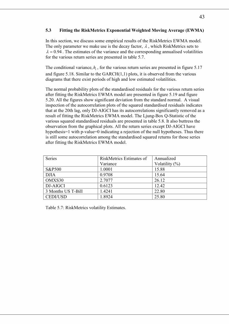
5.3 Fitting the RiskMetrics Exponential Weighted Moving Average (EWMA)

In this section, we discuss some empirical results of the RiskMetrics EWMA model.

The only parameter we make use is the decay factor, λ , which RiskMetrics sets to

0.94λ = . The estimates of the variance and the corresponding annualised volatilities

for the various return series are presented in table 5.7.

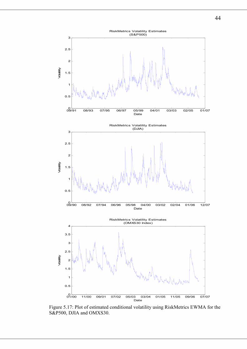
The conditional variance, th , for the various return series are presented in figure 5.17

and figure 5.18. Similar to the GARCH(1,1) plots, it is observed from the various

diagrams that there exist periods of high and low estimated volatilities.

The normal probability plots of the standardised residuals for the various return series

after fitting the RiskMetrics EWMA model are presented in figure 5.19 and figure

5.20. All the figures show significant deviation from the standard normal. A visual

inspection of the autocorrelation plots of the squared standardised residuals indicates

that at the 20th lag, only DJ-AIGCI has its autocorrelations significantly removed as a

result of fitting the RiskMetrics EWMA model. The Ljung-Box Q-Statistic of the

various squared standardised residuals are presented in table 5.8. It also buttress the

observation from the graphical plots. All the return series except DJ-AIGCI have

hypothesis=1 with p-value=0 indicating a rejection of the null hypotheses. Thus there

is still some autocorrelation among the standardised squared returns for those series

after fitting the RiskMetrics EWMA model.

Series RiskMetrics Estimates of

Variance

Annualized

Volatility (%)

S&P500 1.0001 15.88

DJIA 0.9708 15.64

OMXS30 2.7077 26.12

DJ-AIGCI 0.6123 12.42

3 Months US T-Bill 1.4241 22.80

CEDI/USD 1.8924 25.80

Table 5.7: RiskMetrics volatility Estimates.

44

09/91 08/93 07/95 06/97 05/99 04/01 03/03 02/05 01/070

0.5

1

1.5

2

2.5

3

Date

Volatility

RiskMetrics Volatility Estimates

(S&P500)

09/90 08/92 07/94 06/96 05/98 04/00 03/02 02/04 01/06 12/070

0.5

1

1.5

2

2.5

3


(DJIA)

Date

Volatility

01/00 11/00 09/01 07/02 05/03 03/04 01/05 11/05 09/06 07/070

0.5

1

1.5

2

2.5

3

3.5

4


(OMXS30 Index)

Date

Volatility

Figure 5.17: Plot of estimated conditional volatility using RiskMetrics EWMA for the

S&P500, DJIA and OMXS30.

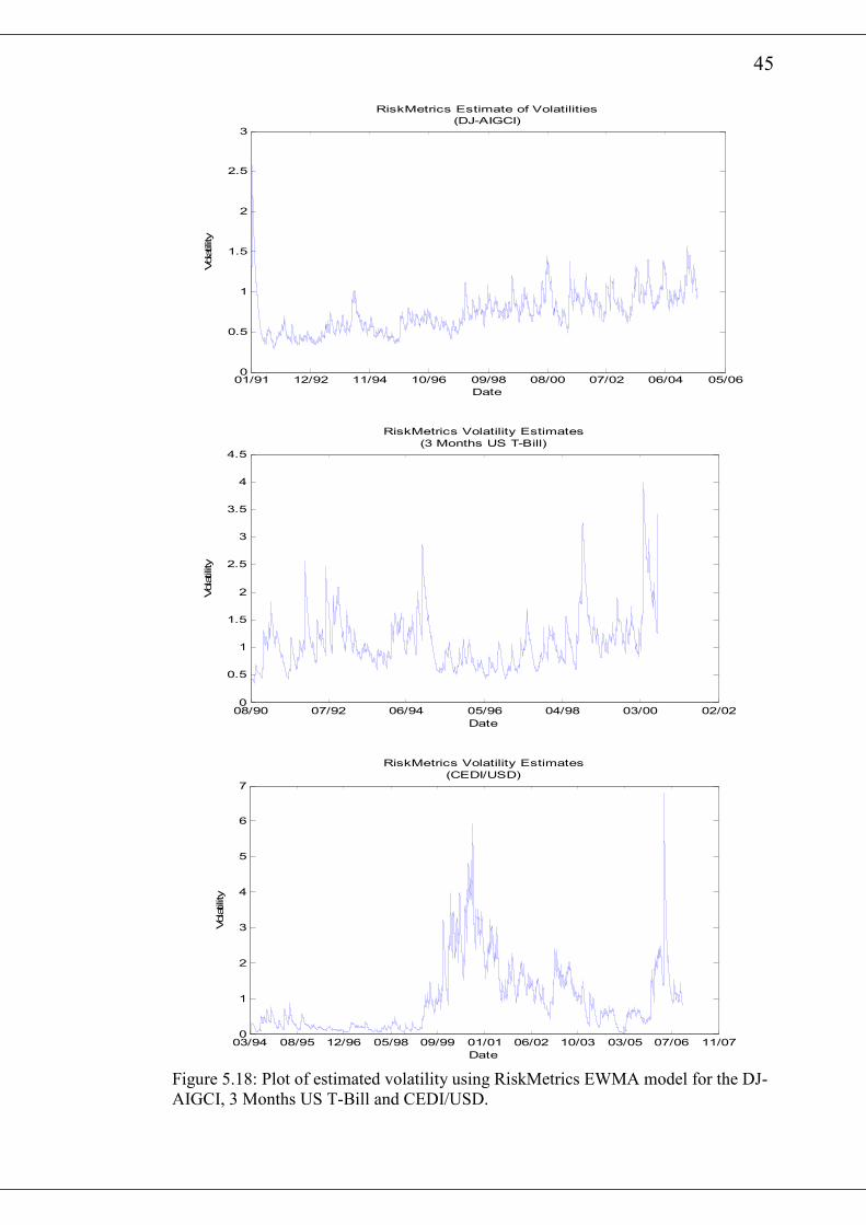
45

01/91 12/92 11/94 10/96 09/98 08/00 07/02 06/04 05/060

0.5

1

1.5

2

2.5

3

RiskMetrics Estimate of Volatilities

(DJ-AIGCI)

Date

Volatility

08/90 07/92 06/94 05/96 04/98 03/00 02/020

0.5

1

1.5

2

2.5

3

3.5

4

4.5



Date

Volatility

03/94 08/95 12/96 05/98 09/99 01/01 06/02 10/03 03/05 07/06 11/070

1

2

3

4

5

6

7

Date

Volatility


(CEDI/USD)

Figure 5.18: Plot of estimated volatility using RiskMetrics EWMA model for the DJ-

AIGCI, 3 Months US T-Bill and CEDI/USD.

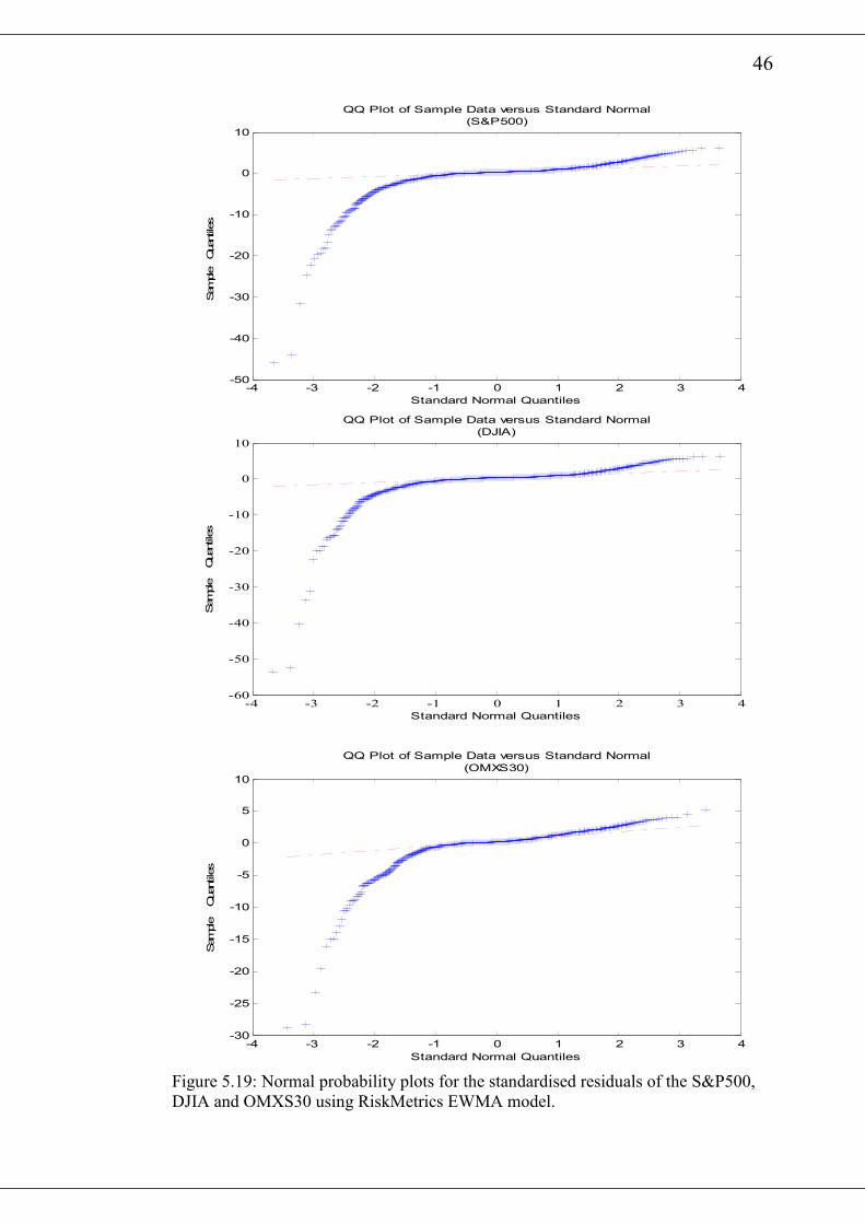
46

-4 -3 -2 -1 0 1 2 3 4-50

-40

-30

-20

-10

0

10


Sample Quantiles


(S&P500)

-4 -3 -2 -1 0 1 2 3 4-60

-50

-40

-30

-20

-10

0

10


Sample Quantiles


(DJIA)

-4 -3 -2 -1 0 1 2 3 4-30

-25

-20

-15

-10

-5

0

5

10


Sample Quantiles


(OMXS30)

Figure 5.19: Normal probability plots for the standardised residuals of the S&P500,

DJIA and OMXS30 using RiskMetrics EWMA model.

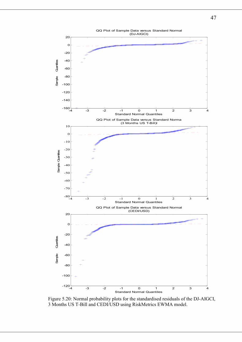
47

-4 -3 -2 -1 0 1 2 3 4-160

-140

-120

-100

-80

-60

-40

-20

0

20


Sample Quantiles


(DJ-AIGCI)

-4 -3 -2 -1 0 1 2 3 4-80

-70

-60

-50

-40

-30

-20

-10

0

10


Sample Quantiles

QQ Plot of Sample Data versus Standard Norma

(3 Months US T-Bill)l

-4 -3 -2 -1 0 1 2 3 4-120

-100

-80

-60

-40

-20

0

20


Sample Quantiles


(CEDI/USD)

Figure 5.20: Normal probability plots for the standardised residuals of the DJ-AIGCI,

3 Months US T-Bill and CEDI/USD using RiskMetrics EWMA model.

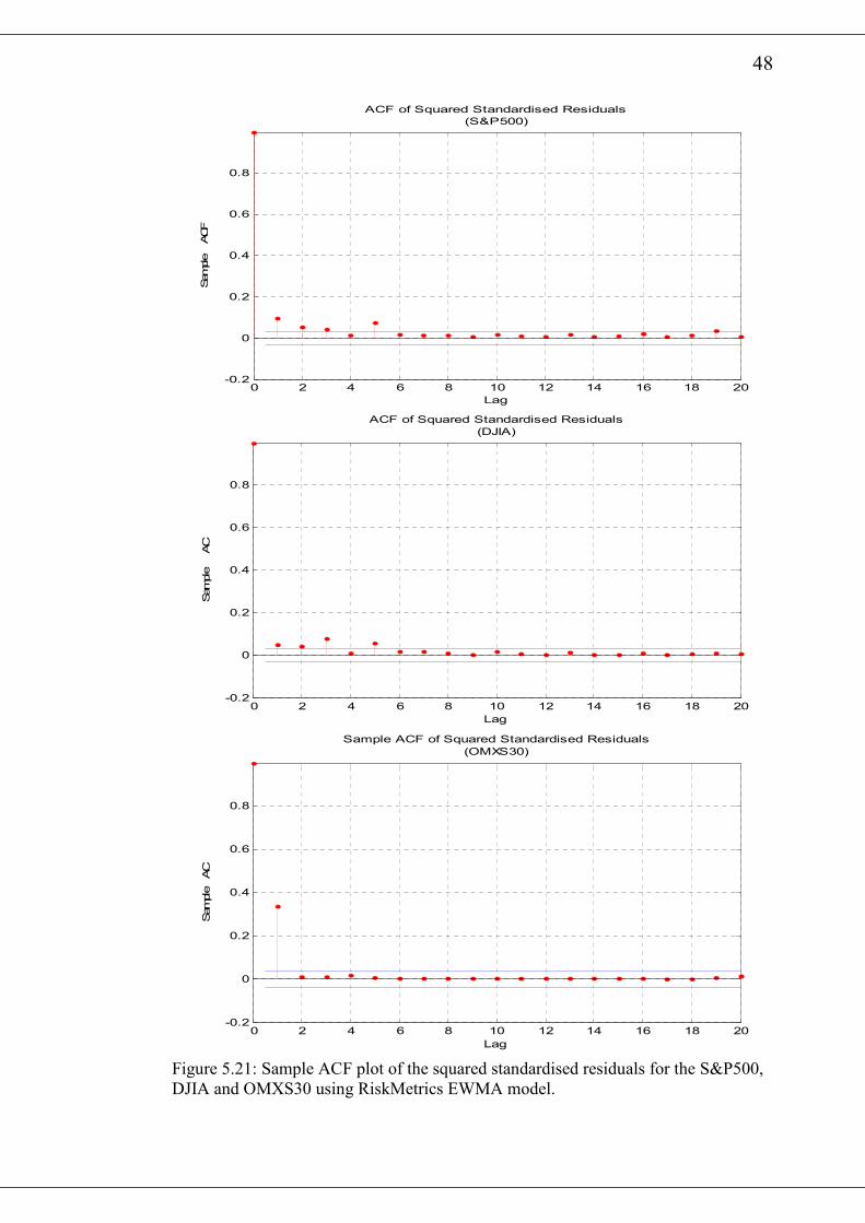
48

0 2 4 6 8 10 12 14 16 18 20-0.2

0

0.2

0.4

0.6

0.8

Lag

Sample ACF

ACF of Squared Standardised Residuals

(S&P500)

0 2 4 6 8 10 12 14 16 18 20-0.2

0

0.2

0.4

0.6

0.8

Lag

Sample AC


(DJIA)

0 2 4 6 8 10 12 14 16 18 20-0.2

0

0.2

0.4

0.6

0.8

Lag

Sample AC

Sample ACF of Squared Standardised Residuals

(OMXS30)

Figure 5.21: Sample ACF plot of the squared standardised residuals for the S&P500,

DJIA and OMXS30 using RiskMetrics EWMA model.

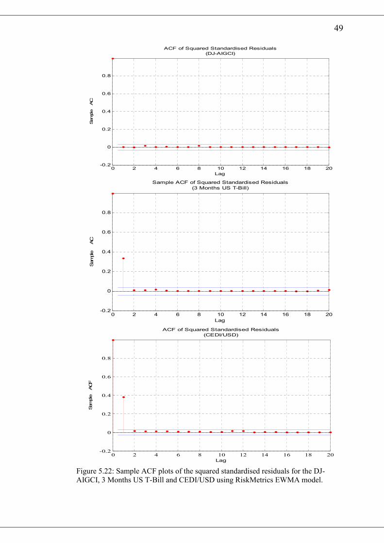
49

0 2 4 6 8 10 12 14 16 18 20-0.2

0

0.2

0.4

0.6

0.8

Lag

Sample AC


(DJ-AIGCI)

0 2 4 6 8 10 12 14 16 18 20-0.2

0

0.2

0.4

0.6

0.8

Lag

Sample AC

Sample ACF of Squared Standardised Residuals


0 2 4 6 8 10 12 14 16 18 20-0.2

0

0.2

0.4

0.6

0.8

Lag

Sample ACF


(CEDI/USD)

Figure 5.22: Sample ACF plots of the squared standardised residuals for the DJ-

AIGCI, 3 Months US T-Bill and CEDI/USD using RiskMetrics EWMA model.

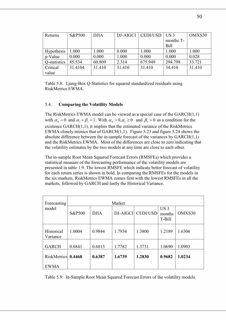
50


months T-

Bill

OMXS30

Hypothesis 1.000 1.000 0.000 1.000 1.000 1.000

p-Value 0.000 0.000 1.000 0.000 0.000 0.028

Q-statistics 85.534 60.809 2.314 675.949 294.798 33.721

Critical

value

31.4104 31.410 31.410 31.410 34.410 31.410

Table 5.8: Ljung-Box Q-Statistics for squared standardized residuals using

RiskMetrics EWMA.

5.4. Comparing the Volatility Models

The RiskMetrics EWMA model can be viewed as a special case of the GARCH(1,1)

with 0 0α = and 1 1 1α β+ = . With 0 10, 0α α> ≥ and 1 0β > as a condition for the

existence GARCH(1,1), it implies that the estimated variance of the RiskMetrics

EWMA closely mimics that of GARCH(1,1). Figure 5.23 and figure 5.24 shows the

absolute difference between the in-sample forecast of the variances by GARCH(1,1)

and the RiskMetrics EWMA. Most of the differences are close to zero indicating that

the volatility estimates by the two models at any time are close to each other.

The in-sample Root Mean Squared Forecast Errors (RMSFEs) which provides a

statistical measure of the forecasting performance of the volatility models are

presented in table 1.9. The lowest RMSFE which indicate better forecast of volatility

for each return series is shown in bold. In comparing the RMSFEs for the models in

the six markets, RiskMetrics EWMA comes first with the lowest RMSFEs in all the

markets, followed by GARCH and lastly the Historical Variance.

Market Forecasting

model S&P500 DJIA DJ-AIGCI CEDI/USD

US 3

months

T-Bill

OMXS30

Historical

Variance

1.0004 0.9844 1.7934 1.3800 1.2189 1.6306

GARCH 0.6841 0.6813 1.7782 1.3731 1.0690 1.0903

RiskMetrics

EWMA

0.4468 0.6387 1.6739 1.2830 0.9682 1.0234

Table 5.9: In-Sample Root Mean Squared Forecast Errors of the volatility models.

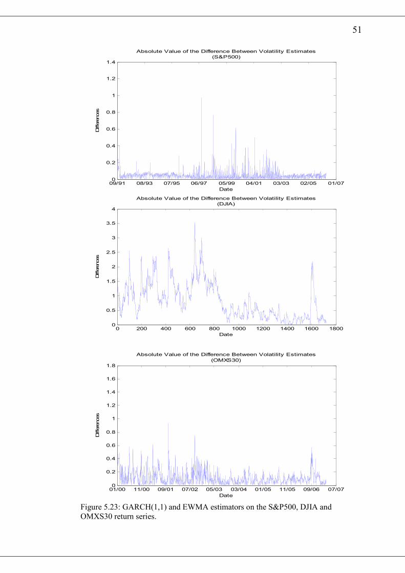
51

09/91 08/93 07/95 06/97 05/99 04/01 03/03 02/05 01/070

0.2

0.4

0.6

0.8

1

1.2

1.4

Absolute Value of the Difference Between Volatility Estimates

(S&P500)

Date

Differences

0 200 400 600 800 1000 1200 1400 1600 18000

0.5

1

1.5

2

2.5

3

3.5

4


(DJIA)

Date

Differences

01/00 11/00 09/01 07/02 05/03 03/04 01/05 11/05 09/06 07/070

0.2

0.4

0.6

0.8

1

1.2

1.4

1.6

1.8


(OMXS30)

Date

Differences

Figure 5.23: GARCH(1,1) and EWMA estimators on the S&P500, DJIA and

OMXS30 return series.

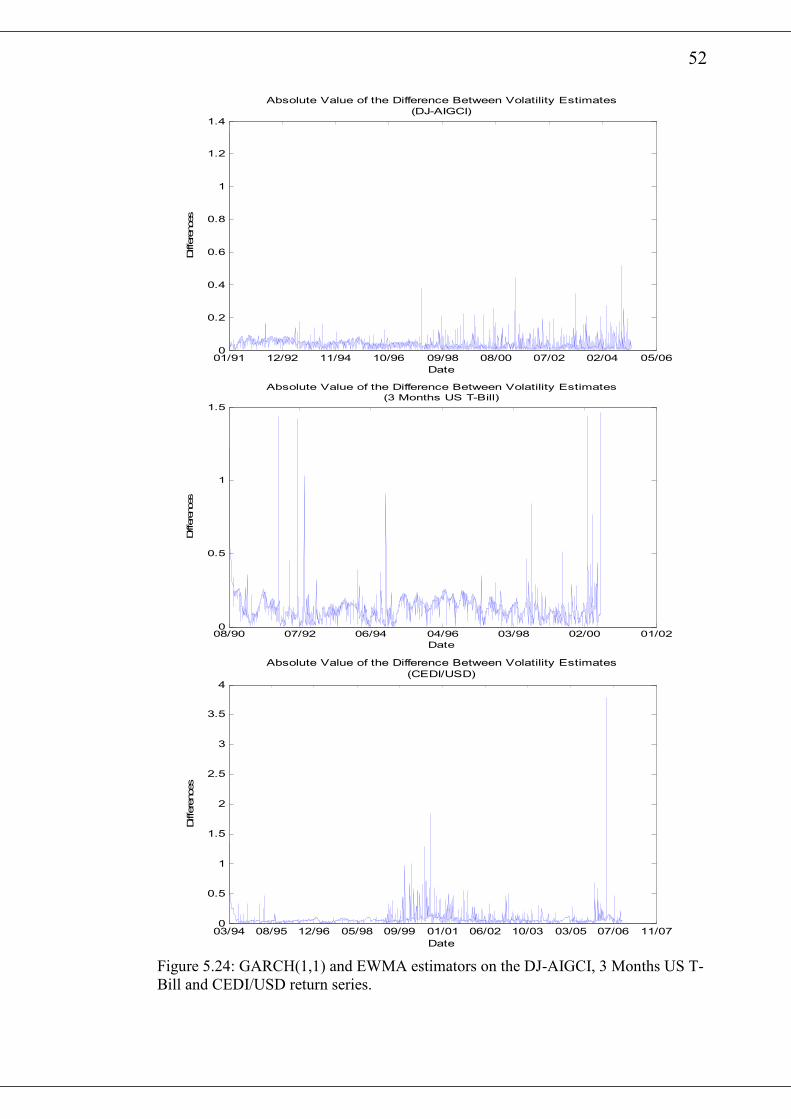
52

01/91 12/92 11/94 10/96 09/98 08/00 07/02 02/04 05/060

0.2

0.4

0.6

0.8

1

1.2

1.4


(DJ-AIGCI)

Date

Differences

08/90 07/92 06/94 04/96 03/98 02/00 01/020

0.5

1

1.5



Date

Differences

03/94 08/95 12/96 05/98 09/99 01/01 06/02 10/03 03/05 07/06 11/070

0.5

1

1.5

2

2.5

3

3.5

4


(CEDI/USD)

Date

Differences

Figure 5.24: GARCH(1,1) and EWMA estimators on the DJ-AIGCI, 3 Months US T-

Bill and CEDI/USD return series.

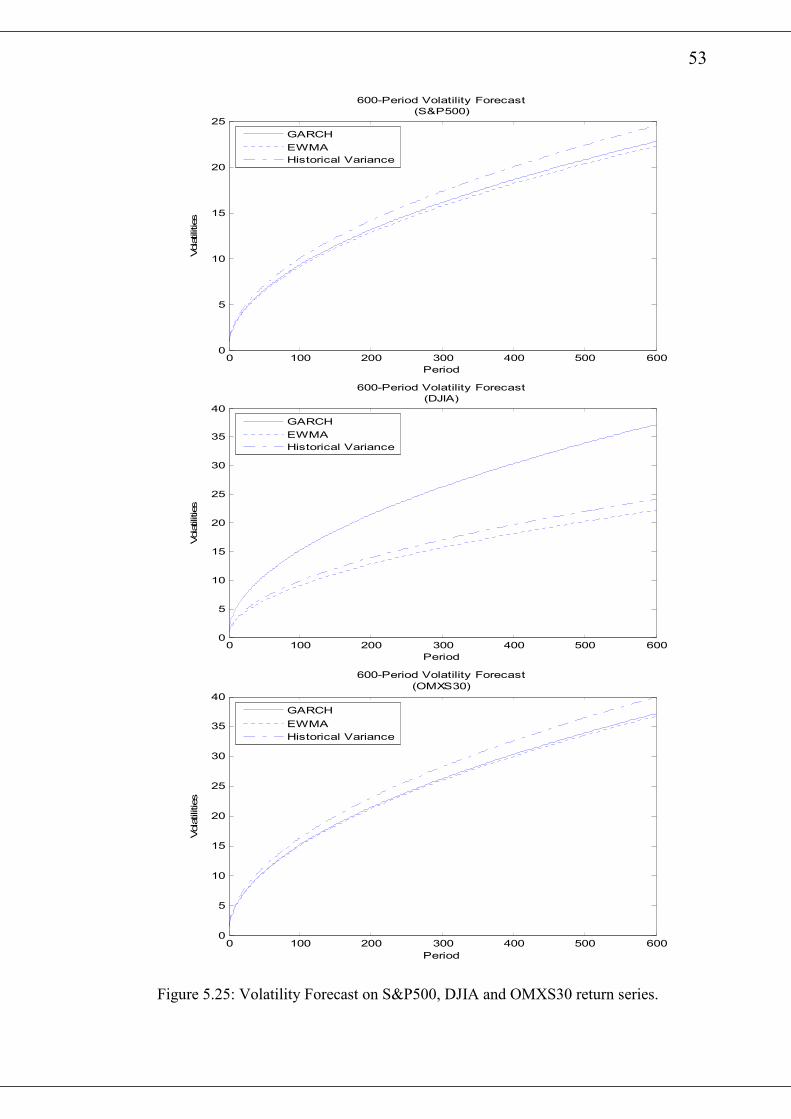
53

0 100 200 300 400 500 6000

5

10

15

20

25

Period

Volatilities

600-Period Volatility Forecast

(S&P500)

GARCH

EWMA

Historical Variance

0 100 200 300 400 500 6000

5

10

15

20

25

30

35

40

Period

Volatilities


(DJIA)

GARCH

EWMA

Historical Variance

0 100 200 300 400 500 6000

5

10

15

20

25

30

35

40

Period

Volatilities


(OMXS30)

GARCH

EWMA

Historical Variance

Figure 5.25: Volatility Forecast on S&P500, DJIA and OMXS30 return series.

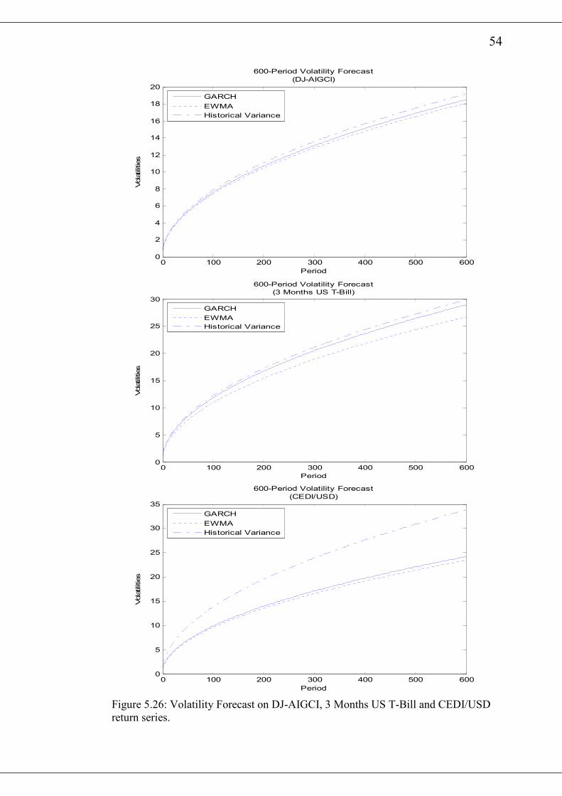
54

0 100 200 300 400 500 6000

2

4

6

8

10

12

14

16

18

20

Period

Volatilities


(DJ-AIGCI)

GARCH

EWMA

Historical Variance

0 100 200 300 400 500 6000

5

10

15

20

25

30

Period

Volatilities



GARCH

EWMA

Historical Variance

0 100 200 300 400 500 6000

5

10

15

20

25

30

35

Period

Volatilities


(CEDI/USD)

GARCH

EWMA

Historical Variance

Figure 5.26: Volatility Forecast on DJ-AIGCI, 3 Months US T-Bill and CEDI/USD

return series.

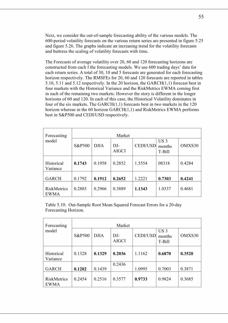
55

Next, we consider the out-of-sample forecasting ability of the various models. The

600-period volatility forecasts on the various return series are presented in figure 5.25

and figure 5.26. The graphs indicate an increasing trend for the volatility forecasts

and buttress the scaling of volatility forecasts with time.

The Forecasts of average volatility over 20, 60 and 120 forecasting horizons are

constructed from each f the forecasting models. We use 600 trading days’ data for

each return series. A total of 30, 10 and 5 forecasts are generated for each forecasting

horizon respectively. The RMSFEs for 20, 60 and 120 forecasts are reported in tables

5.10, 5.11 and 5.12 respectively. In the 20 horizon, the GARCH(1,1) forecast best in

four markets with the Historical Variance and the RiskMetrics EWMA coming first

in each of the remaining two markets. However the story is different in the longer

horizons of 60 and 120. In each of this case, the Historical Volatility dominates in

four of the six markets. The GARCH(1,1) forecasts best in two markets in the 120

horizon whereas in the 60 horizon GARCH(1,1) and RiskMetrics EWMA performs

best in S&P500 and CEDI/USD respectively.

Market Forecasting

model S&P500 DJIA DJ-

AIGCI

CEDI/USD US 3

months

T-Bill

OMXS30

Historical

Variance 0.1743 0.1958 0.2852 1.5554 08318 0.4284

GARCH 0.1792 0.1912 0.2652 1.2221 0.7303 0.4241

RiskMetrics

EWMA

0.2885 0.2966 0.3889 1.1343 1.0337 0.4681

Table 5.10: Out-Sample Root Mean Squared Forecast Errors for a 20-day

Forecasting Horizon.

Market Forecasting

model S&P500 DJIA DJ-

AIGCI

CEDI/USD US 3

months

T-Bill

OMXS30

Historical

Variance

0.1328 0.1329 0.2036 1.1162 0.6870 0.3520

GARCH 0.1202 0.1439 0.2436

1.0995 0.7003 0.3871

RiskMetrics

EWMA

0.2454 0.2516 0.3577 0.9733 0.9824 0.3685

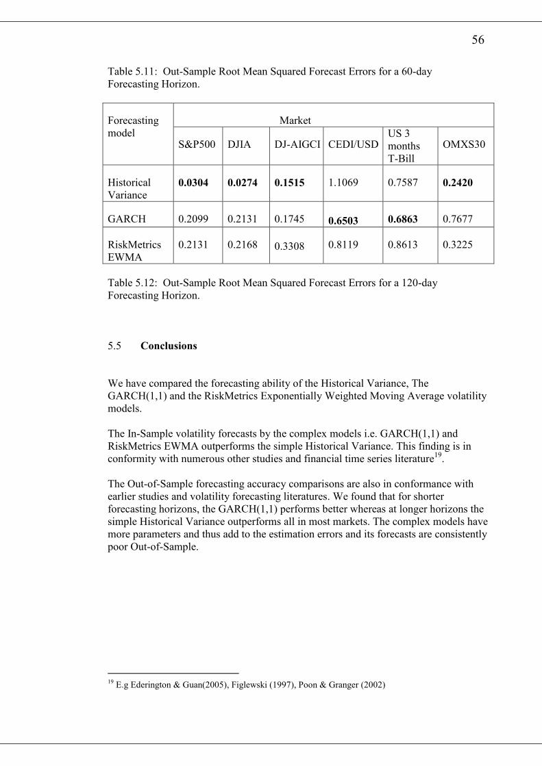
56



Market Forecasting

model S&P500 DJIA DJ-AIGCI CEDI/USD

US 3

months

T-Bill

OMXS30

Historical

Variance 0.0304 0.0274 0.1515 1.1069 0.7587 0.2420

GARCH 0.2099 0.2131 0.1745

0.6503 0.6863 0.7677

RiskMetrics

EWMA

0.2131 0.2168

0.3308 0.8119 0.8613 0.3225



5.5 Conclusions

We have compared the forecasting ability of the Historical Variance, The

GARCH(1,1) and the RiskMetrics Exponentially Weighted Moving Average volatility

models.

The In-Sample volatility forecasts by the complex models i.e. GARCH(1,1) and

RiskMetrics EWMA outperforms the simple Historical Variance. This finding is in

conformity with numerous other studies and financial time series literature19.

The Out-of-Sample forecasting accuracy comparisons are also in conformance with

earlier studies and volatility forecasting literatures. We found that for shorter

forecasting horizons, the GARCH(1,1) performs better whereas at longer horizons the

simple Historical Variance outperforms all in most markets. The complex models have

more parameters and thus add to the estimation errors and its forecasts are consistently

poor Out-of-Sample.

19 E.g Ederington & Guan(2005), Figlewski (1997), Poon & Granger (2002)

57

References

• Beninga S. (2000). Financial Modelling. The MIT Press

• Bickel, P.J and Doksum, K.A. (1977). Mathematical statistics.

Holden-Day San Francisco

• Bollerslev, T. (1986). Generalized Autoregressive Conditional

Heteroscedasticity. Journal of Econometrics 31, 307-327.

• Brockwell P.J. and Davis R.A. (2002). Introduction to Time Series and

Forecasting, second edition, Springer-Verlag, New York.

• Campbell, John Y., Burton Malkiel, Martin Lettau, and Yexiao Xu. (2001).

Have Individual Stocks Become More Volatile? An Empirical Exploration of

Idiosyncratic Risk. Journal of Finance, 56, 1-43

• Ederington, L.H and Guan, W. (2005). Forecasting Volatility. Journal of

Futures Markets. 25, 465-490.

• Engle, R. F. (2003) .Risk and Volatility: Econometric Models and Financial

Practice. Nobel Lecture. nobelprize.org/nobel_prizes/economics/laureates/2003/engle-

lecture.pdf

• Engle, R. F. and Paton, A. J. (2001). What good is a volatility Model?

Quantitative Finance 1, 237-245.

• Figlewski, S. (1997). Forecasting Volatility. Financial Markets, Institutions

and Instruments 6 (1), 1-88.

• Lamoureux, C.B and Lastrapes, W.D. (1993). Forecasting Stock Return

Variance: Toward an Understanding of Stochastic Implied Volatilities, Review

of Financial Studies 6, 293-326.

• LJUNG, G.M and BOX G.E.P (1978). Biometrika. 65(2), 297-303

• Luenberger, D.G. (1997) - Investment Science. Oxford University

Press, Inc, New York.

• J.P Morgan and Reuters. (1996). RiskMetrics-A technical document, New

York, Dec 1996.

• Jorion P. (1997). Value at Risk: The New Benchmark for Controlling Market

Risk. McGraw-Hill Companies Inc.

• Poon S.H and Granger C.W.J (2002), Forecasting Volatility in Financial

Markets - Journal of Economic Literature 41, 478-539.

• Taylor S. (1986). Modelling Financial Time Series. John Wiley & sons.

• Xu, X and Taylor, S.J.(1995). Conditional Volatility and Informational

Efficiency of the PHLX Currency Options Market. Journal of Banking &

Finance. 5, 803-821.

58

Appendix

A.1 Aggregation Property of the Normal Distribution

The aggregation property of the normal distribution implies that the sum of jointly

normal random variables is also normal. This property underlines the RiskMetrics

assumption that portfolio’s return is the weighted sum of the underlying assets,(see

equation (17)).

Let , , 1,2,...,i tr i N= be the returns of the underlying assets of a portfolio then the

return on the portfolio is given by

, ,

1

N

p t i i t

i

r w r=

=∑ . (A1.1)

The portfolio returns has mean

,

1

N

p t i i

i

wµ µ=

=∑ ,

where ,( )i i tE rµ = . RiskMetrics models each return , , 1,2,...,i tr i N= as a random walk

as in equation (19) i.e.

, , ,i t i i t i tr µ σ ε= + . (A1.2)

Assume that the errors ,i tε are distributed as multivariate normal

( , )t tMVN Rε µ∼ , 1, 2, ,, ,...,t t N tε ε ε ε = (A1.3)

where tR is the correlation matrix of the errors , , 1, 2,...,i t i Nε = . In view of the

property that the sum of jointly normal random variables is normal, the portfolio return

,p tr is normally distributed with mean ,p tµ and variance 2

,p tσ given by

2

,

, 1

N

p t i j ij

i j

wwσ σ=

=∑ (A1.4)

A.2 Test for Conditional Normality

The quantile-quantile plot or for short Q-Q plot is used as a graphical check on the

deviation of the data from normality. The chart shows a plot of the quantiles of the

standardized distribution of the observed returns against the quantiles of the standard

normal distribution. A distribution is normal if the plot is a straight line whereas a

deviation from normality is characterize by deviation from the straight line.

59

In addition to the graphical inspection, a quantitative method can be used to calculate

the correlation coefficient of the Q-Q plot,

1

2 2

1 1

( )( )

( ) ( )

T

j j

j

QT T

j j

j j

q q r r

q q r r

ρ =

= =

− −

=

− −

∑

∑ ∑ (A2.1)

At 5% significant level, one needs 0.999Qρ ≥ for normality test to hold under a large

sample size, T.

A.3 The RiskMetrics k-period (day) Volatility Forecast

We derive here the k-period volatility forecast for a single asset whose return is

conditional normal as a proof of equations (35) and (36). This derivation can be

generalized for an n-dimensional case where the assets follow a conditional

multivariate normal distribution.

For the RiskMetrics model, the one-day log-price return ( , 1)t t + is assumed to follow

the dynamics

1 1 1t t tr σ ε+ + += (A3.1)

where

2 2 2

1 (1 )t t trσ λσ λ+ = + − (A3.2)

and [0,1]λ∈ . By definition, 1tσ + is measurable w.r.t tψ , and the error terms tε are

assumed to be N(0,1) and independent of the information at time t. The k-day return is

given by

,

1

k

t t k t i

i

r r+ +=

=∑ , (A3.3)

hence from equation (A3.1) it follows that

,

1

k

t t k t i t i

i

r σ ε+ + +=

=∑ . (A3.4)

The expected return for the k-days at time t is

60

,

1

( | ) ( | )k

t t k t t i t i t

i

E r Eψ σ ε ψ+ + +=

=∑

1

1

[ ( | ) | ]k

t i t i t i t

i

E E σ ε ψ ψ+ + + −=

=∑

( )1

1

[| ( | ) | ]k

t i t i t i t

i

E Eσ ε ψ ψ+ + + −=

=∑

1

[ ( | )]k

t i t i t

i

E Eσ ε ψ+ +=

=∑

0= (A3.5)

and the corresponding variance is

( )2

, , ,( | ) [ ( | )] |t t k t t t k t t k t tVar r E r E rψ ψ ψ+ + += −

2

,( | )t t k tE r ψ+=

2

1

[ ] |k

t i t

i

E r ψ+=

=

∑

, 1

( | )k

t i t i t j t j t

i j

E σ ε σ ε ψ+ + + +=

=∑ . (A3.6)

It is obvious that for i j≠ , the expectation vanishes. Assume for example that

1 i j≤ < , then

1( | ) [ ( | ) | ]t i t i t j t j t t i t i t j t j t j tE E Eσ ε σ ε ψ σ ε σ ε ψ ψ+ + + + + + + + + −=

( )1[ ( | ) | ]t i t i t j t j t j tE Eσ ε σ ε ψ ψ+ + + + + −=

[ ( ) | ]

0

t i t i t j t j tE Eσ ε σ ε ψ+ + + +=

= (A3.7)

This holds for i j> also because of symmetry.

For 1i j= ≥ , we have

2 2 2 2

1( | ) [ ( | ) | ]t i t i t t i t i t i tE E Eσ ε ψ σ ε ψ ψ+ + + + + −=

( )2 2

1

2 2

2

[ ( | ) | ]

[ ( | )]

[ | ].

t i t i t i t

t i t i t

t i t

E E

E E

E

σ ε ψ ψ

σ ε ψ

σ ψ

+ + + −

+ +

+

=

=

=

(A3.8)

Substituting this result into equation (A3.6), we get

2

,

1

( | ) [ | ].k

t t k t t i t

i

Var r Eψ σ ψ+ +=

=∑ (A3.9)

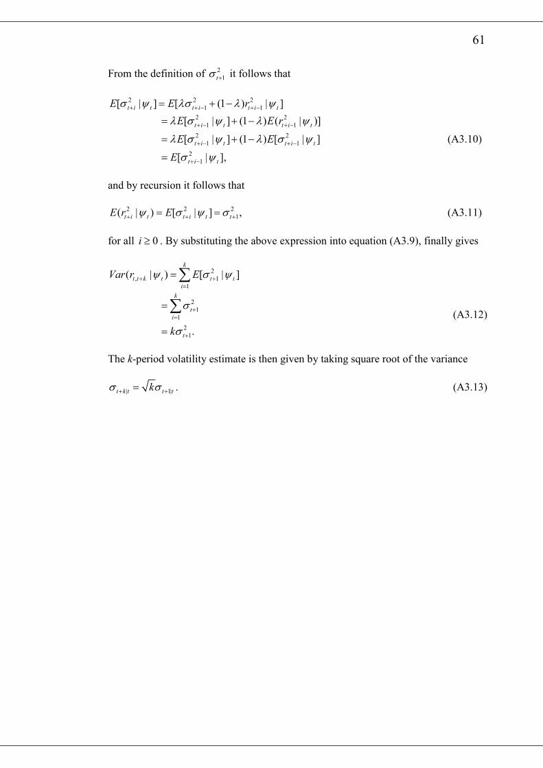
61

From the definition of 2

1tσ + it follows that

2 2 2

1 1[ | ] [ (1 ) | ]t i t t i t i tE E rσ ψ λσ λ ψ+ + − + −= + −

2 2

1 1

2 2

1 1

2

1

[ | ] (1 ) ( | )]

[ | ] (1 ) [ | ]

[ | ],

t i t t i t

t i t t i t

t i t

E E r

E E

E

λ σ ψ λ ψ

λ σ ψ λ σ ψ

σ ψ

+ − + −

+ − + −

+ −

= + −

= + −

=

(A3.10)

and by recursion it follows that

2 2 2

1( | ) [ | ] ,t i t t i t tE r Eψ σ ψ σ+ + += = (A3.11)

for all 0i ≥ . By substituting the above expression into equation (A3.9), finally gives

2

, 1

1

( | ) [ | ]k

t t k t t t

i

Var r Eψ σ ψ+ +=

=∑

2

1

1

2

1.

k

t

i

tk

σ

σ

+=

+

=

=

∑ (A3.12)

The k-period volatility estimate is then given by taking square root of the variance

| 1|t k t t tkσ σ+ += . (A3.13)

forecasting volatility - diva portal304496/fulltext01.pdf · forecasting volatility volatility...

Documents