volatility forecasting in financial risk management with

Volatility Forecasting in Financial Risk Management with Statistical Models and ARCH-RBF Neural Networks

Dusan Marcek Research Institute of the IT4I Centre of Excellence, Faculty of Philosophy and Sciences, Silesian University in Opava

Bezruc Square 13, Opava 74601, Czech Republic E-mail: [email protected]

Lukas Falat The Faculty of Management Science and Informatics, University of Zilina

Univerzitna 8215/1, Zilina 01026, Slovakia E-mail: [email protected]

Abstract

As volatility plays very important role in financial risk management, we investigate the volatility dynamics of EUR/GBP currency. While a number of studies examines volatility using statistical models, we also use neural network approach. We suggest the ARCH-RBF model that combines information from ARCH with RBF neural network for volatility forecasting. We also use a large number of statistical models as well as different optimization techniques for RBF network such as genetic algorithms or clustering. Both insample and out-of-sample forecasts are evaluated using appropriate evaluation measures. In the final comparison none of the considered models performed significantly better than the rest with respect to the considered criteria. Finally, we propose upgrades of our suggested model for the future.

Keywords: volatility, forecasting, ARCH-RBF, EUR/GBP, currency, risk in management.

1. Introduction

The recent global financial crisis has highlighted the need for financial institutions to find and implement appropriate models for risk quantification. Therefore, volatility estimates were subject to research in this domain.

There are more reasons why to forecast volatility – volatility is extremely important for risk management, for asset allocation, and for taking bets on future volatility. A large part of risk management is measuring the potential future losses of a portfolio of assets (volatility modelling provides a simple approach to calculating value at risk of a financial position in risk management), and in order to measure these potential losses, estimates must be made of future volatilities and

correlations. In asset allocation, the Markowitz approach of minimizing risk for a given level of expected returns (see Ref. 1) has become a standard approach, and of course an estimate of the variance-covariance matrix is required to measure risk. Perhaps the most challenging application of volatility forecasting, however, is to use it for developing a volatility trading strategy. Option traders often develop their own forecast of volatility, and based on this forecast they compare their estimate for the value of an option with the market price of that option. The simplest approach to estimating volatility is to use historical standard deviation, but there is some empirical evidence, which we will discuss later, that this can be improved upon.

Various approaches to volatility modelling have been suggested in the econometric and financial

Journal of Risk Analysis and Crisis Response, Vol. 4, No. 2 (June 2014), 77-95

Published by Atlantis Press Copyright: the authors

77

willieb

Typewritten Text

Received 8 December 2013

willieb

Typewritten Text

Accepted 16 April 2014

D. Marcek, L. Falat

literature. In the following we will provide a brief overview of developments in the literature starting with the autoregressive conditional heteroskedasticity (ARCH) models (Ref. 2). Bollerslev (Ref. 3) introduced the generalised ARCH (so called GARCH) model. Later, as time went on, many extensions of the GARCH model have been introduced in the literature since: e.g. GARCH-in-mean (GARCH-M) models (Ref. 4), EGARCH models (Ref. 5), Threshold ARCH (TARCH) and Threshold GARCH (TGARCH) (Ref. 6) and Power Arch (PARCH) models (Ref. 7) just to name a few. A number of studies have focused on optimal model specification and the performance of various GARCH models in financial markets providing no clear-cut results (such as Ref. 8).

Also, as computer science has developed, techniques of machine learning started to apply in the domain of financial forecasting. Gooijer and Hyndman (Ref. 9) proved that artificial neural networks had the biggest potential in time series forecasting. Therefore, various types of neural networks have been used for forecasting future values of high frequency financial data such as (Ref. 10) or (Ref. 11).

This study examines various models that can be used in forecasting volatility, to evaluate their respective performance. One of the main reasons for finding the appropriate volatility model is that volatility, as a representation of risk, plays an important role in an investor’s decision making process. Volatility is not only of great concern for investors but also policy makers and regulators who are interested in the effect of volatility on the stability of financial markets in particular and the whole economy in general. Finally, volatility estimation is an essential input in many VaR (Value at Risk) models, as well as for a number of applications in a firms market risk management practices.

This paper concerns with forecasting volatility and it is divided into eight chapters. Chapter two deals with volatility in risk management and how uncertainty impacts the decision-making process. Chapter three presents the statistical ARCH/GARCH models used for volatility forecasting. In chapter four, data we use for our tests are presented. In chapter five we perform the GARCH volatility modelling on our tested data and in chapter six we present the neural network approach as

well as our ANN model for volatility forecasting. In chapter seven the results are discussed.

2. Volatility and Uncertainty in Risk Management

As for risk management, the complexity of managerial decision-making relates to decision-making with incomplete information. Most of the real systems can only be described incompletely, i.e. with information which cannot be formally expressed by set parameters. Uncertain information makes it impossible to exactly determine the future behaviour of the system. This type of uncertainty is called stochastic and is concerned with the category of the probability risk (Ref. 12).

However, evidence shows that it is possible to reduce this type of stochastic uncertainty by a suitable choice and use of forecasting models. These models based on statistical and soft computing methods or artificial intelligence methods are capable of providing information in the form of forecasts of quantities with an acceptable degree of uncertainty.

Managers using these forecasts are able to make better decisions, i.e. such decisions whose risks in achieving targets are minimized. To realize that Cox and Hinkley and Weisberg (see Refs. 13 and 14) suggested the theory of point estimates and confidence intervals. The confidence interval indicates the span of possible values into which falls the future estimate of the forecasted quantity with the chosen probability defined by the manager. This way the limits of the possible future values are set. Point or interval estimates of the future values of various economic indicators are important for the strategic manager's decision-making. When determining information entropy in decision-making, it is useful to focus on how the confidence interval for the forecasted economic quantity can be made more precise, i.e. narrowed by using the forecasting model. This kind of uncertainty is in forecasting models based on the standard deviation (also called volatility in financial domain) which is widely used in measuring risks of forecasts of various (mainly economic) time series (see e.g. Refs. 15 and 16). The standard deviation as a degree of uncertainty or risk of forecasted quantity values estimates is proportional to the statistical degree of accuracy of the forecast defined as Root Mean Square Error (RMSE). This approach is


78

Volatility Forecasting in Risk Management

used with measuring risks of forecasts of many economic and financial forecasting models, and is also used in managing financial risk (Value at Risk models). However, not to be confused, standard deviation (or volatility) does not reflect entropy in its true substance as uncertainty which is indicated in bits. Uncertainty is closely related to how precise are the forecasts (estimates of the future values) that managers have at their disposal. Important to note, the strong prerequisite for the application of such a model in management is that apart from the increased reliability of decision-making, the model output results in uncertainty reduction, which makes decision-making easier and less weighted with risk. The facilitation of manager's decision-making process is not sufficient.

Resulting from the arguments stated above, accurate volatility forecasting is extremely important in risk management, mainly in financial domain.

3. Volatility Forecasting - ARCH and GARCH Models

In this chapter, we are going to look at the statistical models which are able to capture and model stochastic financial volatility, i.e. to capture the autocorrelation of squared returns, the reversion of volatility to the mean, as well as the excess kurtosis.

The major breakthrough in the history of statistical modelling came with publishing a study from Box & Jenkins (Ref. 17). In this study authors integrated all the knowledge including autoregressive and moving average models into one book. From that time the ARIMA (AutoRegressive Integrated Moving Averages) models have been very popular in time series modelling for a long time as O'Donovan (Ref. 18) showed that these models provided better results than other models used in that time. It is therefore no surprise that for more than 20 years Box-Jenkins ARMA models have been widely used for time series modelling. The models published in (Ref. 17) are autoregressive models (AR) and moving average (MA) models. Let yt be a stationary time series that is a realization of a stochastic process. Then, general formula of ARMA(p,q) model can be expressed as follows

∑ ∑= =

−− −++=p

i

q

jjtititit yy

1 1εθεφξ

(1)

where ξ is a constant, ,....),( 21 φφ are autoregressive

parameters, ,....),,( 21 −− ttt εεε are independent random parts. If the model is correct, residuals are to form the white noise process. The model is composed of two parts –autoregressive (determnistic) part expressing the linear dependence on previous values of the dependent variable yt; and stochastic part represented by moving averages.

If the series is not stationary, ARIMA models must be used. Let yt be a time series and let d be the order of differentation; yt will be called ARIMA(p,d,q) process if its dth differences produce ARMA(p,q) process. ARIMA can be formally defined as

ttd ByBB εμ )()1)(( Θ+=−Φ (2)

It is also obvious that if d equals zero, ARIMA equals just simple ARMA process. The whole process of Box-Jenkins statistical modelling, which is performed through Box-Jenkins analysis, has more steps and it is described in details in (Ref. 3).

Risk is an important characteristics in currency and financial trading. As we already know, the most common way in expressing the risk is the volatility. Financial volatility, which is present in dynamic economic markets like stock market or forex market and which plays an important role in financial forecasting as well as financial risk analysis, has some very unique features. First of all, it is its stochastic character. Moreover, financial time series exhibit a characteristic known as volatility clustering in which large changes tend to follow large changes, and small changes tend to follow small changes. Volatility is hence clustered in time and therefore it has persistance character. Resulting from this, actual variance is dependent on the previous variances and the time series is characterized by the time-variant conditional variance, also called clustering of variances.

Another feature of financial volatility is mean reversion. Volatility is often persistent and so has a long memory. In the long term period the volatility oscilates around its long-term mean which results in the fact that all long-term forecasts are to converge to its long-term mean value. So even though financial time series can exhibit excessive volatility sometimes, volatility will finally settle down to a long run level.

It has been also experimentally proved that the distribution of many high frequency financial time series usually have fatter tails than a Gaussian


79

D. Marcek, L. Falat

distribution. A phenomenon of fatter tails is also called as excess kurtosis.

The weakness of ARIMA models in modeling financial time series is the inability to model stochastic non-constant volatility having the features we described above. In (Ref. 2) Engle suggested the solution by creating so called ARCH (Autoregressive Conditional Heteroskedastic) models which assume heteroskedastic variance of tε . Let yt be a standard stationary AR(p) process defined as in (1) and let at be a random part of this model and hence, is a white noise process and has a constant unconditional variance. Let also assume that

1|| <iφ for i = 1, 2, ... p. According to Engle (see Ref. 2), the model will

become more confident and the predictions will be more precise if it is dependent on a conditional variance of tε

t

p

iitit yy εφ += ∑

=−

1 (3)

where the expected value of tε is zero tε and can be transformed into the form

ttt he=ε (4)

where tε is the residual part of the model having mean value equaled to zero, et is a white noise process ~ N(0,1) and ht is a function of conditional heteroskedastic variance of random part defined as follows

∑=

−+=p

jjtjth

1

20 εαα (5)

According to (Ref. 2), the standard ARCH model of p order is defined by equations (4) and (5) and should be used for conditional variance modeling. The conditional variance in the ARCH(p) model is a function of the past squares of random variable et (which can be understood as an arrival of new information in particular time moments). The ARCH model described above is able to model the basic properties of financial volatility such as volatility clustering, stochastic properties of volatility, mean reversion, fat tails etc.

Bollershev (Ref. 3) suggested the generalized form of ARCH model called GARCH (Generalized Autoregressive Heteroskedastic Models) where conditional variance of ht depends on the previous conditonal variances. The general GARCH(p,q) model can be formally defined as

ttt he=ε (6)

it

p

ii

q

jjtjt hh −

==− ∑∑ ++=

11

20 βεαα (7)

where { tε }is a sequence of error parts, {et} is a white noise process and ht is a function of conditional variance. It is also necessary that jα > 0, j = 1,2,...,q. and 0≥iβ for i = 1,2,...,p.

There exists a number of GARCH extensions, each of them are used to model some unusual property of volatility. EGARCH created by Nelson (Ref. 5) is an implementation of leverage effects. As assymetric influence of new information is another feature of financial volatility. EGARCH is able to model this feature of volatility. The leverage effect implemented in EGARCH expresses the asymmetric impact of positive and negative changes in financial time series. It means that the negative shocks in price influence the volatility differently than the positive shocks at the same size. This effect appears as a form of negative correlation between the changes in prices and the changes in volatility. EGARCH models leverage effects in the form

∑∑=

−= −

−− ++

+=q

jjtj

p

i it

itiitit hh

110

||log β

σεγε

αα (8)

The leverage effect is present as follows: if tε is positive (there is ”good news”), the total effect of it−ε is iti −+ εγ )1( . However, if it−ε is negative (there is so called ”bad news”), the total effect of it−ε is

||)1( iti −− εγ . Resulting from this, in EGARCH model bad news usually have larger impact on the volatility. (value of would be expected to be negative). For details see (Ref. 19).

The basic GARCH model can be also extended to allow for leverage effects. This is performed by treating the basic GARCH model as a special case of the power GARCH (PGARCH) model proposed by Ding, Granger and Engle (see Ref. 7):

∑∑=

−=

−− +++=q

j

djtj

dp

iitiiti

dt

110 )|(| σβεγεαασ (9)

where d is a positive exponent. Before (G)ARCH modeling, one has to find out if

heteroskedasticity is really present in series. According to Engle (Ref. 2), the presence of heteroskedasticity is tested by ARCH test which supposes a non-existence of


80


ARCH. This tests uses the Lagrange Multiplier (LM) statistics (Ref. 19).

4. Empirical Data

As risk analysis plays a very important role at financial institutions all over the world we decided to apply our models to forex market. Forex is one of the most dynamic market in the world and its data are often very dynamic, extremely volatile and sometimes chaotic (Ref. 20). These features seem to be a good base for testing our models. This paper focuses on financial time series of daily close prices of EUR/GBP exchange rate.

Fig. 1. Time Series of daily close prices of EUR/GBP currency (October, 2003 – October, 2013).

The data we used, covered the historical period from October 31, 2003 to October 31, 2013 (n = 2610 daily observations). * The graphical characteristics of the series is illustrated in Figure 1. Due to validation of our models, data were divided into two parts. The first part included 1306 observations (from 10/31/2008 to 10/31/2008) and was used for training (quantification) of our models. The second part of data (11/1/2008 to 10/31/2013), counting 1304 observations, was used for model validation by making one-day-ahead ex-post forecast. These observations included new data which had not been incorporated into model estimation. We used so many data in the validation phase in order to guarantee the validation robustness of our models. The reason for validation was to find out the real prediction power of the models; there was an assumption that if the

* The data was downloaded from the website http://www.global-view.com/forex-trading-tools/forex-history.

model could handle to predict data from ex-post set, it would be able to predict values of a currency pair in the real future.

Finally, in order to evaluate the characteristics for quantified model as well as to compare the real forecasting performance of our proposed models, the numerical characteristic for assessing models called Mean Squared Error (MSE) was used.

∑=

+−+−

∧− ⎟

⎠⎞

⎜⎝⎛ −=

H

hhHnhHn YYHMSE

1

21

(10)

where h is the forecasting horizon, H is the total number of predictions for the horizon h over the forecast period, ∧Y is the estimated value and Y is the original value of the series.

5. Empirical Statistical Analysis and ARCH Modelling

The empirical statistical analysis, which was performed according to Box-Jenkins (Ref. 17), focused on the original and differentiated series of daily observations of EUR/GBP currency pair covering a historical period from October 31, 2003 to October 31, 2008. Figure 2 and Figure 3 illustrates the original series as well as differences of the training set respectively. As stated in the previous section, we only used observations from training set for statistical modeling. Statistical modelling was performed in the Eviews software.

Fig. 2. EUR/GBP – training set (original series).


81

D. Marcek, L. Falat

Fig. 3. Differences of EUR/GBP series – training set.

Unit root tests results (see Refs. 21, 22, 23, 24) presented in the Table 4 (Appendix A) showed that this series was not stationary. In order to stationarize the series, it was differentiated. As seen from the Table 4, unit root tests confirmed that the differentiated series became stationary which had been a necessary condition in Box-Jenkins modelling.

By analyzing autocorrelation (ACF) and partial autocorrelation functions (PACF) of the differentiated series of EUR/GBP (see Table 5, Appendix A), there were no significant correlation coefficients (on alpha = 0.05). Due to that we supposed that first differences of the original series formed a white noise process. In that case, the original series would have formed random walk process (RWP) as RWP is I(1) process. Assuming the differences of the original series formed a white noise process, we selected AR(0) as the basic Box-Jenkins model. Ljung-Box Q-statistics (see Table 5, right side) confirmed this assumption and the applicability of AR(0) process as the correlations were statistically not significant.

However, the assumption of normality of residuals of AR(0) was rejected at 0.05 significance level (see Table 5, Appendix A). The observed assymetry might have indicated the presence of nonlinearities in the evolution process of residuals. This nonlinearity was also confirmed by graphical quantiles comparison (see Figure 4) and a scatter plot of the series which did not appear to be in the form of a regular ellipsoid (see Figure 5). In addition, BDS test rejected the random

walk hypothesis (see Table 7 Appendix A) as the BDS statistic was greater than the critical value at 0.05 level.

Fig. 4. Quantiles of EUR/GBP residuals vs Fig. 6 Scatter plot of EUR/GBP residuals the Normal distribution quantiles.

Fig. 5. Scatter plot of EUR/GBP residuals variations.

Therefore, other tests had to be performed in order to correctly model this series.

We noted that the residuals of AR(0) (see Figure 6) were not characterized by a Gaussian distribution (see Table 6, Appendix A). The assymetry might have indicated non-linearities in the residuals. When looking


82


at the graph of residuals (see Figure 6), one could observe the variability of these residuals could have been caused by the non-constant variance. Residual with small value followed another residuals with a small value. On the other hand, residual with a large value usually followed a residual with another large value. However, this is not typical for a white noise process. Therefore, this assumption lead us to think about stochastic model for volatility.

Fig. 6. Evolution of residuals of AR(0) model.

The suitability for using stochastic volatility model was also accepted by performed heteroskedasticity test. ARCH test (see Table 6, Appendix A) confirmed the series was heteroskedastic since the null hypothesis of homoskedasticity had been rejected at 5% and so the residuals were characterized by the presence of ARCH effect which was quite a frequent phenomenon at financial time series. Therefore, we applied a stochastic volatility model into the basic model. According to correlogram of squared residuals of EUR/GBP differences (see Table 8, Appendix A) we quantified ARCH(4) model for volatility.

After quantification of ARCH(4) model, the residuals were characterized by the absence of conditional heteroskedasticity: the ARCH-LM statistics were strictly less than the critical value at 5%. In addition, the standardized residuals tested with Ljung-Box Q-test (see Table 9, Appendix A) confirmed there were no significant coefficients in residuals of this model. Finally, the final ARCH(4) volatility model is defined as follows

24

23

22

21

2

085457.0150503.0

101053.0104930.000000438.0

−−

−−

++

++=

tt

tt

εε

εεσ (11)

Table 10 in Appendix A states the numerical characteristics of ARCH(4) model as well as Student’s t-statistics for its parameters.

6. Neural Network Approach in Volatility Forecasting

In the recent years, other techniques started to apply in the domain of time series forecasting. One of the reason was the study by Bollershev (Ref. 3), where he proved the existence of nonlinearity in financial data. Non-linearity modelling was one of the drawbacks of Box-Jenkins models. Today, according to studies such as that by Gooijer (Ref. 9), artificial neural networks (ANN) are the machine learning models having the biggest potential in forecasting financial time series. This is due to the fact that these models are extremely helpful in modelling non-linear processes which have a priori unknown functional relations or this system of relations is very complex to describe mathematically (see Ref. 25).

ANN is based on human neural system and is an universal functional black-box approximator of non-linear type (Ref. 26, 27 and 28). The reason for attractiveness of ANNs for financial prediction can be found in the work of Hill et al. (Ref. 29). Here, the authors showed that the ANNs worked best in connection with highfrequency financial data. The competitive performance of ANN is also documented on a large number of time series (see Refs. 30 and 31). In this part we show a new approach of estimation of forecasting function for conditional volatility modelled by feedforward neural network of RBF type combined with genetic algorithms as well as statistical ARCH models.

A fully connected feed forward neural network was selected to be used as the forecasting function, due to its conceptual simplicity, and computational efficiency (Ref. 32). Our implemented neural network consisted of three layers, except for the input and output, there was also one hidden layer. We proposed the architecture of the neural network (see Figure 7) with only one hidden layer due to the fact that according to Cybenko theorem


83

D. Marcek, L. Falat

(Ref. 33) the network with one hidden layer is able to approximate any continuous function. This hidden layer made a previous nonlinear transformation of the data so as to facilitate resolution of the problem in hand such as regression, classification, etc. The neural network used for this research was the network of RBF type (Ref. 34). This network is one of the most frequently used networks for regression (Ref. 32). RBF, as well as multilayer perceptron (MLP, which is a predecessor of RBF) have been widely used to capture a variety of nonlinear patterns (see Ref. 35) thank to their universal approximation properties (see Ref. 36); in other words, thanks to their capacity to approximate any continuous function provided that they have a sufficient number of hidden units (neurons).

Fig. 7. The architecture of used RBF neural network.

The structure of our RBF neural network is defined by its architecture (processing units and their interconnections, activation functions, methods of learning and so on). In Figure 7 each circle or node represents the neuron. The neural network consisted of an input layer with input vector x and an output layer with the output value ty .

The layer between the input and output layers is normally referred to as the hidden layer and its neurons as RBF neurons. Here, the input layer is not treated as a layer of neural processing units. One important feature of RBF networks is the way how output signals are

calculated in computational neurons. The output signals of the hidden layer are

)(2 jjo wx −=ψ (12)

where x is a k-dimensional neural input vector, jw

represents the hidden layer weights, 2ψ are radial basis (Gaussian) activation functions. Note that for an RBF network, the hidden layer weights jw represent the

centres jc of activation functions in the hidden layer.

The second parameter of the radial basis function, the standard deviation, is estimated as K, (K ≥ 1) multiple of the mean value of quadratic distance among the input vectors and their cluster centres. The value of K is regarded as the rate of overlapping in the distribution of input data (see Ref. 37).

The output layer neuron is linear and has a scalar output given by

y = ∑=

s

jjjov

1 (13)

where jv are the trainable weights connecting the component of the output vector o . Then, the output of the hidden layer neurons are the radial basic functions of the proximity of weights and input values. A serious problem is how to determine the number of hidden layer (RBF) neurons. The most used selection method is to preprocess training (input) data by some clustering algorithm. After choosing the cluster centres, the shape parameters jσ must be determined. These parameters express an overlapping measure of basis functions. For Gaussians, the standard deviations jσ can be selected,

i.e. jσ ~ scΔ , where scΔ denotes the average distance among the centres.

Finally, the RBF network computed the output data set as

ty = ),,( vcx tG = ∑=

s

jjttjv

12, ),( cxψ = ∑

=

s

jtjjov

1,

t = 1, 2, ..., N (14)

where N is the size of data samples, s denotes the number of the hidden layer neurons. The hidden layer neurons received the Euclidian distances )( jcx − and computed the scalar values tjo , of the Gaussian function ),(2 jt cxψ that form the hidden


84


layer output vector to . Finally, the single linear output layer neuron computed the weighted sum of the Gaussian functions that formed the output value of ty .

In order to optimize the outputs of the network and to maximise the accuracy of the forecasts, we had to optimize parameters of ANN. The most popular method for learning (i.e. adapting parameters) in multilayer networks is called back-propagation invented by Bryson and Ho (Ref. 38).

However, there are some drawbacks to back-propagation. One of them is the convergence of this algorithm - it generally converges to any local minimum on the error surface, since stochastic gradient descent exists on a surface which is not flat. Due to this reason, we also used the combination of back-propagation with the standard unsupervised technique called K-means (see Ref. 39). K-means algorithm, which belongs to a group of unsupervised learning methods, is a nonhierarchical exclusive clustering method based on the relocation principle. The most common type of characteristic function is location clustering. The K-means was used in the phase of non-random initialization of weight vector w performed before they were adapted by back-propagation. i.e. before the phase of network learning. We assumed that in many cases it was not necessary to interpolize the output value by radial functions, it was quite sufficient to use one function for a set of data (cluster), whose center was considered to be a center of activation function of a neuron. We also supposed that after K-means performed, weights should have been located near the global minimum of the error function and lower number of epochs were supposed to be used for network training.

The values of centroids were used as an initialization values of weight vector w. To find the weights jw or centres of activation functions we used the following adaptive (learning) version of K-means clustering algorithm for s clusters:

Step 1. Randomly initialise the centres of RBF neurons )(t

jc, j = 1, 2, …, s (15)

where s represents the number of chosen RBF neurons (clusters).

Step 2. Apply the new training vector )(tx = ).,...,,( 21 kxxx (16)

Step 3. Find the nearest centre to )(tx and replace its position as follows

)1( +tjc = )(t

jc + λ(t) ( )(tx - )(tjc ) (17)

where λ(t) is the learning coefficient and is selected as linearly decreasing function of t by λ(t) = λ0(t) (1 - t/N) where λ0(t) is the initial value, t is the present learning cycle and N is number of learning cycles.

Step 4. After chosen epochs number, terminate learning. Otherwise go to step 2

The above learning method based on the clustering algorithm is regarded as one of the granular method presenting the bottom-up granulation (see Ref. 40). Input vectors are combined into larger overlaping granules (clusters) described by cluster´s centres and the standard deviations.

Since back-propagation also features some other problems such as “scaling problem" we decided to implement genetic algorithm as an learning technique for our RBF neural network too. Therefore, in our implementation of ANN, back-propagation was altered by the genetic algorithm (GA) as an alternative learning technique in the process of weights adaptation. Adopted from biological systems, genetic algorithms, which are algorithms for optimization and machine learning, are stochastic search techniques that guide a population of solutions towards an optimum using the principles of evolution and natural genetics (Ref. 41). They are based loosely on several features of biological evolution (Ref. 42), have become a popular optimization tool in various areas. They require five components to be met (Ref. 43):

1. A way of encoding solutions to the problem on chromosomes. In the original genetic algorithm an individual chromosome is represented by a binary string. The bits of each string are called genes and their varying values alleles. A group of individual chromosomes is called a population.

2. An evaluation function which returns a rating for each chromosome given to it.

3. A way of initializing the population of chromosomes.

4. Operators that may be applied to parents when they reproduce to alter their genetic composition. Standard operators are mutation and crossover (i.e. recombination of genetic material).

5. Parameter settings for the algorithm, the


85

D. Marcek, L. Falat

operators, and so forth. Genetic algorithms are characterized by basic

genetic operators which include reproduction, crossover and mutation (Ref. 44). Given these genetic operatos and five components stated above, a genetic algorithm operates according to the following steps (Ref. 45):

1. Initialize the population using the initialization procedure, and evaluate each member of the initial population.

2. Reproduce until a stopping criterion is met. Reproduction consists of iterations of the following steps:

a) Choose one or more parents to reproduce. Selection is stochastic, but the individuals with the hightest evaluations are usually favored in the selection.

b) Choose a genetic operator and apply it to the parents.

c) Evaluate the children and accumulate them into a generation. After accumulating enough individuals, insert them into the population, replacing the worst current members of the population.

When the components of the genetic algorithm are

chosen appropriately, the reproduction process should continually generate better children from good parents. The algorithm can then produce populations of better and better individuals, converging finally on results close to a global optimum. Additionally, GA can efficiently search large and complex (i.e., possessing many local optima) spaces to find nearly a global optima (Ref. 45).

In addition to that, genetic algorithm does not have the same problem with scaling as back-propagation. One reason for this is that it generally improves the current best candidate monotonically. It does this by keeping the current best individual as part of their population while they search for better candidates. Moreover, supervised learning algorithms suffer from the possibility of getting trapped on suboptimal solutions. Genetic algorithms are generally not bothered by local minima. The mutation and crossover operators can step from a valley across a hill to an even lower valley with no more difficulty than descending directly into a valley. So GA enables the learning process to

escape from entrapment in local minima in instances where the back-propagation algorithm converges prematurely.

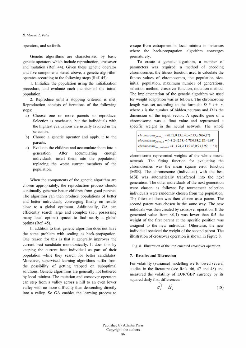
To create a genetic algorithm, a number of parameters was required: a method of encoding chromosomes, the fitness function used to calculate the fitness values of chromosomes, the population size, initial population, maximum number of generations, selection method, crossover function, mutation method. The implementation of the genetic algorithm we used for weight adaptation was as follows. The chromosome length was set according to the formula: D * s + s, where s is the number of hidden neurons and D is the dimension of the input vector. A specific gene of a chromosome was a float value and represented a specific weight in the neural network. The whole

chromosome represented weights of the whole neural network. The fitting function for evaluating the chromosomes was the mean square error function (MSE). The chromosome (individual) with the best MSE was automatically transferred into the next generation. The other individuals of the next generation were chosen as follows: By tournament selection individuals were randomly chosen from the population. The fittest of them was then chosen as a parent. The second parent was chosen in the same way. The new indiduals was then created by crossover operation. If the generated value from <0,1) was lower than 0.5 the weight of the first parent at the specific position was assigned to the new individual. Otherwise, the new individual received the weight of the second parent. The illustration of crossover operation is shown in Figure 8.

Fig. 8. Illustration of the implemented crossover operation.

7. Results and Discussion

For volatility (variance) modelling we followed several studies in the literature (see Refs. 46, 47 and 48) and measured the volatility of EUR/GBP currency by its squared daily first differences:

22yt Δ=

∧

σ (18)


86


Proof. From the chapter five we know that the differenced series is an ARMA(0,0) process; therefore:

ty ε=Δ (19)

Let define vt as the error between the square residuals and the variance

22tttv σε −= (20)

according to ARCH process

∑=

−+=p

iitit

1

20

2 εαασ (21)

∑=

−+=−p

iititt v

1

20

2 εααε (22)

ttt v+= 22 σε , vt ~ iid(0,1) (23)

hence

22yt Δ=

∧

σ (24)

In our tests, we used one-step-ahead, frequently

called as static, forecasts, i.e. the horizon of predictions was equal to one day. As we said, we used MSE (Mean Square Error) and RMSE (root mean square error) numerical characteristics for assessing all models.

Firstly, we estimated and tested the ARCH(4) model for volatility defined in (11). However, we also tested some other statistical models modelling conditional variance such as GARCH(1,1) model (Ref. 2) which is supposed to be so-called universal model in financial domain. We also tested EGARCH(1,1,1) defined in (8). Important to remember that the estimation of these models was only based on 1306 in-sample observations, in order to make ex-ante predictions with remaining 1304 observations. We used the Marquardt optimization procedure for finding the optimal values of ARCH/GARCH parameters. Initial values of parameters were counted using Ordinary Least Squares (OLS) method and these values were then optimized by iterative process constisted of 500 iterations. Convergence rate was set to 0.0001. The forecasting ability of particular networks was measured by the MSE criterion of ex post forecast periods (validation data set).

As for models based on neural networks, we implemented three models, each of them was an implementation of feedforward neural network of RBF type (Ref. 34). In addition to that we implemented three

different optimization techniques for adaptation of weights (parameters) of this network – genetic algorithm, standard back-propagation algorithm (BP) as well as a combination of K-means clustering combined with the back-propagation (KM+BP). We implemented all of these algorithms and models by ourselves using the JAVA programming language. The approximation as well as forecasting results measured by MSE were calculated analogously as in the case of ARCH/GARCH models.

As for the inputs into our ANN models, we used the information from the statistical models, particularly from ARCH(4). Looking at the equation of the ARCH(4) model we knew that the conditional variance was dependent on the previous four lagged squared residuals. Therefore we used this information to construct a hybrid neural network (so called ARCH-RBF neural network) which used the residuals from ARCH(4) model to compute the outputs (variance). This approach is shown in Figure 9.

Fig. 9. The suggested and implemented model of ARCH-RBF neural network.

For adaptation via BP we used learning rate of 0.1, 0.05 respectively. As for adaptive K-means, we used 10000 cycles and the learning rate of K-means adaptation was set to 0.1, 0.05 respectively. The number of clusters was set to the number of hidden neurons.

We also tested several configurations of genetic algorithms with different population size, different mutation rates as well as size of the first choice process. For this particular data the best mutation rate showed to be 0.1, 0.2 respectively. If performed, the specific gene (weight) of a chromosome was changed to a random value. The best population sizes were 500 and 1000


87

D. Marcek, L. Falat

individuals. The first choice crossover was set with probability p1=0.02 and the second one with p2 = 0.5. The results for in-sample predictions are stated in Table 1 and results for out-of-sample predictions (ex-post predictions) are stated in Table 2.

Table 1. Prediction accuracy of tested models measured by MSE (in-sample predictions).

Learning method RBF configuration RBF (BP) RBF (KM) RBF (GA)

(4 – 3 – 1) 5,3664*10-3 2,4832*10-10 2,5547*10-10

(4 – 5 – 1) 46933*10-3 2,2493*10-10 2,4505*10-10

(4 – 7 – 1) 2,6660*10-10 1,9481*10-9 5,5255*10-10

(4 – 10 – 1) 1,6411*10-2 4,5823*10-9 3,0536*10-10

Error Distribution Statistical model Gaussian Student GED

ARCH(4) 2,2350*10-10 2,2360*10-10 2,2353*10-10

GARCH(1,1) 2,1718*10-10 2,1726*10-10 2,1722*10-10

EGARCH(1,1,1) 2,1644*10-10 2,1642*10-10 2,1643*10-10

Table 2. Prediction accuracy of tested models measured by MSE (out-of-sample predictions).

Learning method RBF configuration RBF (BP) RBF (KM) RBF (GA)

(4 – 3 – 1) 4,1471*10-9 3,9282*10-9 4,2028*10-9

(4 – 5 – 1) 4,1590*10-9 4,2222*10-9 4,1587*10-9

(4 – 7 – 1) 4,2156*10-9 1,1480*10-8 4,1170*10-9

(4 – 10 – 1) 4,5086*10-9 7,8121*10-9 4,9923*10-9

Error Distribution Statistical model Gaussian Student GED

ARCH(4) 3,8203*10-9 3,8054*10-9 3,8143*10-9

GARCH(1,1) 3,5058*10-9 3,5175*10-9 3,5099*10-9

EGARCH(1,1,1) 3,4809*10-9 3,4836*10-9 3,4851*10-9

The standard back-propagation algorithm for

weights adaptation showed to be a weakness of the network. The convergence was really slow (cca 5000 epochs) and in addition to that, resulting from many experiments with learning rate and the initialization by random weights, it generally converged to any local minimum on the error surface. Therefore there was no guarantee that the algorithm would converge to global minimum. In addition, this algorithm was very dependent on the initialized random weights. Due to this, generally a lot of more epochs was needed to achieve reasonable accuracy compared to K-means + BP.

Bearing in mind these disadvantages of BP, we also tested K-means, that was used in the phase of non-random initialization of weight vector w performed

before the phase of network learning. Besides lower MSE at lower configurations of hidden neurons (three, five), another advantage of using K-means upgrade (but also GA) was the consistency of predictions. The standard deviation of these methods was uncomparably lower than the standard deviation when using the standard back-propagation. Moreover, the biggest strength of K-means was in the speed of convergence of the network. Without K-means, it took considerably longer time to achieve the minimum. However, when the K-means was used, the time (number of epochs) for reaching the minimum was much shorter (cca 500 to 1000 epochs). Therefore, the advantage of using K-means together with back-propagation is in the speed of adaptivity rather than in better predictions. However, one must bear in mind that K-means is a relatively efficient algorithm only in the domain of non-extreme values. Otherwise, other advanced non-hierarchical clustering algorithms must be used.

Having tested also genetic algorithm in weights adaptation, we found out the convergence was also considerably faster than at back-propagation. In addition to that, genetic algorithm did not have the same problem with scaling as back-propagation. One reason for this is that GA generally improves the current best candidate monotonically. It does this by keeping the current best individual as part of their population while they search for better candidates.

However, the acuuracy results were not very different from the other two optimization techniques; in some cases the optimization methods based on BP were even more accurate. As according to the theory, genetic algorithms are not bothered by local minimum problem (since the algorithms operate on a population instead of a single point in the search space, they climb many peaks in parallel and therefore reduce the probability of finding local minima) such as BP and as GA are also especially capable of handling problems in which the objective function is discontinuous or non differentiable, nonconvex, multimodal or noise; we expected better results than we got. This could, however, be caused due to non-optimized parameters of GA. Except for our experiments and tests with the best configuration of GA parameters, we also tested the optimization procedure stated in (Ref. 49) which was in our case not very helpful. Maybe, testing some other optimization procedure for the best parameters of GA would lead to


88


better results of genetic algorithm. The second reason could be that the standard unbiased crossover function was used. The biased crossover function stated in (Ref. 45) could enhance our solution.

It is also to mention that the best results were achieved with lower number of neurons. Following from that one can deduce that for remembering the relationships in this time series it is enough to use smaller number of hidden neurons.

The final comparison of statistical as well as neural networks models is stated in Table 3.

Table 3. Final Comparison of out-of-sample (ex-post) predictions.

Numerical characteristics Model MSE E RMSE E Rank

RBF (4 - 3 – 1) (BP) 4,1471*10-9 0,00006439 6 RBF (4 - 3 – 1) (KM) 3,9282*10-9 0,00006267 4 RBF (4 - 7 – 1) (GA) 4,1170*10-9 0,00006416 5 ARCH(4) (Student) 3,8054*10-9 0,00006168 3 GARCH(1,1) (Gauss) 3,5058*10-9 0,00005920 2

EGARCH(1,1,1) (Gauss) 3,4809*10-9 0,00005899 1 Deducing from Table 3, we can say that on the

validation set the best results were achieved with EGARCH(1,1,1) model. On the other hand, the worst results were achieved with RBF neural network combined with the standard back-propagation algorithm. However, the differences between the results were very small and the difference in results between the best and worst model is only about nine per cent.

Following from that, our suggested RBF hybrid neural network combined with ARCH inputs showed to be an efficient and accurate way of forecasting conditional volatility in financial domain. But, generally speaking, the statistical models achieved a little bit higher accuracy than the neural networks models. However, the difference was very small and the results were almost of the same accuracy. However, the achieved ex post accuracy of ARCH-RBF (best RMSE = 0.00006267) is still reasonable and acceptable for use in forecasting volatility which plays an important role in managerial decision processes in the finance area. Moreover, a little bit worse results of neural network models can be the result of the following factors:

• non-optimized parameters of genetic algorithm, which could cause a little bit worse final solution than expected

• back-propagation as the non-ideal optimization technique for parameters optimization

• The non-ideals inputs coming from the statistical ARCH(4) model

• The data we chose for our experiments were not “representative“. One can not eliminate the assumption saying that if we used other data for our experiments the neural network models would outperform the ARCH/GARCH models. Coming from that, there are more options of how to

upgrade this model in the future: 1) We could better „optimize“ the parameters of

genetic algorithm. We could apply other known optimization procedure than (Ref. 49) into our neural network models. It could improve the solution quite a lot.

2) Apart from the standard back-propagation algorithm it would be reasonable to use and implement the more advanced version of this algorithm (to avoid the imprisonment in the local minum). We could use some of the versions of adaptive back-propagation.

3) Probably the outputs of the neural network models would be more accurate if we did not use the inputs from ARCH model. We could use only the information from ARCH model and the residuals would come from the RBF itself. It could be done by implemeting a version of recurrent ARCH-RBF neural network.

4) Probably, even better results could be achieved by implementing the recurrent RBF neural network based on GARCH model, not ARCH (so called recurrent GARCH-RBF).

5) The RBF model could be enhanced by implementing error-correction part, i.e. smoothing the error (residual) of the RBF neural network by using m-period weighted or exponential or simple moving average such as:

,ttRBFt ue +=ε )1,0(iidut ≈ (25)

and

,1∑=

−=q

i

RBFitite εθ ∑

=

=q

ii

11θ (26)


89

D. Marcek, L. Falat

8. Conclusion

In risk management, finding appropriate models for risk quantification is a must. Therefore it is no surprise that volatility forecasting have been subject to research in this domain. The main reason for forecasting volatility for risk managers is that volatility is extremely important. It is due to the fact that a large part of risk management is measuring the potential future losses of a portfolio of assets (and volatility modelling provides a simple approach to calculating value at risk of a financial position in risk management), and in order to measure these potential losses, estimates must be made of future volatilities. Therefore, appropriate models for volatility dynamics in these markets are of great interest to financial risk managers all over the world.

In this paper, we investigated the modelling of volatility dynamics of EUR/GBP exchange rate differences. We examined two types for volatility forecasting – the models based on statistics and neural network models. We evaluated the effectiveness of various volatility models with respect to forecasting market risk in the exchange rate market, EUR/GBP more specifically. While there is a stream of literature examining performance of models for volatility based on statistical approach, this is a pioneer study to particularly focus on forecasting volatility with neural networks.

For all our tests, the data were divided into training set and validation set. The models were quantified only on training set and then they were tested on out-of-sample prediction interval to evaluate their prediction power. The out-of-sample period, that has been tested in this study contained data from November, 1, 2008 to October, 31, 2013. The reason for doing that was that models that perform well in the considered out-of-sample period may well underperform in future periods, particularly when market conditions change. Both in-sample and out-of-sample forecasts were evaluated using statistical summary measures of model’s forecast accuracy.

As for statistical models, we evaluated three most common models for volatility forecasting – the universal GARCH model, the basic ARCH and EGARCH model which is able to model leverage effects. In addition to that, all three models were

evaluated with Gaussian, Student and GED error distrubutions.

In case of models based on neural network approach, we suggested new model for forecasting volatility with neural networks – the ARCH-RBF neural network. We used the proxy metrics to calculate the actual volatility and so we were able to implement the neural network with inputs from the quantified ARCH model and developed the new approach for forecasting volatility. Moreover, we constructed ARCH-RBF neural network with three different types of optimization techniques. Except for the standard back-propagation, we combined an K-means clustering into the RBF to achieve higher accuracy of the network. Both of the algorithms were used in the process of adapting weights of the network. The reason for incorporating other algorithms into the network was that the back-propagation was considered a weakness of the RBF. In addition, we also eliminated the back-propagation algorithm by using the genetic algorithm instead. In the final comparison of the selected optimization techniques both of these upgrades showed to be helpful in the process of creating more accurate forecasts of volatility and they should be definitely used instead of the standardy back-propagation.

According to results we achieved, the statistical approach was better than the neural network models. However, the differences in accuracy of volatility forecasting were very small. None of the considered models performed significantly better than the rest with respect to the considered criteria. So the achieved ex post accuracy of ARCH-RBF neural network models is still reasonable and acceptable for use in forecasting systems that routinely predict volatility in managerial decision processes in the financial domain. Moreover, a little bit higher error could be caused by non-optimizing parameters of genetic algorithm, non-ideal inputs of ARCH model or just due to type of data we used.

On the other hand, there is definitely a reason for using ARCH-RBF neural network in the domain of volatility forecasting as this model showed to be a good tool in volatility forecasting. Neural networks are capable of providing information in the form of forecasts with an acceptable degree of uncertainty. They are relatively fast and have the ability to generalize. Moreover, the ARCH-RBF has such attributes as computational efficiency, simplicity, and ease adjusting


90


to changes in the process being forecast. ARCH/GARCH models require more costs of development, installation and operation in a management system, management comprehension and cooperation, and often a lot of computational time.

Finally, accuracy of our suggested model could be improved by upgrading the model by some of the upgrades we discussed in the Results & Discussion chapter (such as recurrent version of ARCH-RBF, GARCH-RBF, Error-correction RBF, etc). There is a strong assumption that this upgrade can cause this model to have even a great accuracy advantage over the statistical models. We leave the investigation of these issues to future work. Acknowledgements

This paper has been elaborated in the framework of the IT4Innovations Centre of Excellence project, reg. no. CZ.1.05/1.1.00/02.0070 supported by Operational Programme 'Research and Development for Innovations' funded by Structural Funds of the European Union and state budget of the Czech Republic. References

1. H. M. Markowitz, Portfolio Selection, The Journal of Finance, 7 (1) 1952, 77–91.

2. R. F. Engle, Autoregressive Conditional Heteroskedasticity with Estimates of the Variance of United Kingdom Inflation, Econometrica, 50(4) (1982) 987 – 1008.

3. T. Bollershev, Generalized Autoregressive Conditional Heteroskedasticity, Journal of Econometrics, 31 (1986) 307–327.

4. R. F. Engle, D. M. Lilien, R. P. Robins, Estimating time varying risk premia in the term structure: the ARCH-M model, Eonometrica, 55(2) (1987) 391-407.

5. D. B. Nelson, Conditional Heteroskedasticity in Asset Returns: a New Approach, Econometrica, 59 (2) (1991) 347-370.

6. L. R. Glosten, R. Jagannathan, D. E. Runkle, On the relation between the expected value and the volatility of the normal excess return on stocks, The Journal of Finance, 48(5) (1993) 1779-1801.

7. Z. Ding, C. W. Granger, R. F. Engle, A Long Memory Property of Stock Market Returns and a New Model, Journal of Empirical Finance, 1 (1993) 83-106.

8. P. R. Hansen, A. Lunde, A forecast comparison of volatility models: does anything beat a GARCH (1,1). Journal of applied econometrics, 20(7) (2005) 873-889.

9. J. G. Gooijer, R. J. de Hyndman, 25 years of time series forecasting, International Journal of Forecasting, 22 (2006) 443-473.

10. G. P. Zhang, Time series forecasting using a hybird ARIMA and neural network model, Neurocomupting, 50 (2003) 159-175.

11. D. Marcek, Granular RBF NN Approach and Statistical Methods Applied to Modelling and Forecasting High Frequency Data, International Journal of Computational Intelligence Systems, 2 (4) (2009) 353-364.

12. C. F. Huang, D. Ruan, Fuzzy risks and an updating algorithm with new observation, Risk Analysis, 28(3) (2009) 681-94.

13. D. Cox D, D. Hinkley, Teoretical Statistics (Chapman and Hall, London, UK, 1974).

14. S. Weisberg, Applied Linear Regression (Wiley, New York, USA, 1980).

15. D. Applebaum, D. Lévy, Processes and Stochastic Calculus (Cambridge University Press, Cambridge 2004).

16. D. Marcek, Risk Scenes Of Managerial Decision-Making With Incomplete Information: An Assessment In Forecasting Models Based On Statistical And Neural Networks Approach, Journal of Risk Analysis and Crisis Response, 3 (1) (2013) 13-21.

17. G. E. P. Box, G. M. Jenkins, Time series analysis: forecasting and control, (Holden-Day, San Fransisco, 1976).

18. T. M. O'Donovan, Short Term Forecasting: An Introduction to the Box- Jenkins Approach (Wiley, New York, NY, 1987).

19. E. Zivot, J. Wang, Modeling Financial Time Series with S-PLUS (Springer Verlag, NY, 2005).

20. S. A. M. Yaser, A. F. Atiya, Introduction to financial forecasting, Applied Intelligence; 6 (1996) 205–213.

21. D. Dickey, W. Fuller, Distribution of the estimators for autoregressive time series with a unit root. Journal of the American Statistical Association, 74 (1979) 427-431.

22. G. Elliott, T. J. Rothenberg, J. H. Stock, Efficient tests for an autoregressive unit root, Econometrica, 64(4) (1996) 813-836.

23. D. Kwiatkowski, P. Phillips, P. Schmidt, Y. Shin, Testing the null hypothesis of stationary againts the alternative of a unit root; How sure are we that economic time series have a unit root?, Journal of Economics , 54 (1992) 159-178.

24. P. C. B. Phillips, P. Perron, Testing for unit roots in time series regression. Biometrika, 75 (1988) 335-346.

25. G. A. Darbellay, M. Slama, Forecasting the short-term demand for electricity: Do neural networks stand a better chance?, International Journal of Forecasting, 16 (2000) 71– 83.

26. K. Hornik, Some new results on neural network approximation, Neural Networks, 6 (1993) 1069-1072.


91

D. Marcek, L. Falat

27. K. Hornik, M. Stinchcomber, H. White, Multilayer feedforward networks are universal approximations, Neural Networks, 2 (1989) 359-366.

28. L. S. Maciel, R. Ballina, Design a Neural N etwork for Time Series Financial Forecasting: Accura cy and Robustness Analysis (2008)

29. T. L. Hill, M. Marquez, R. O’Connor, Neural networks models for forecasting and decision making, International Journal of Forecasting, 10 (1994) 5-15.

30. K. P. Liao, R. Fildes, The accuracy of a procedural approach to specifying feedforward neural networks for forecasting, Computers & Operations Research, 32 (2005) 2151-2169.

31. G. P. Zhang and M. Qi, Neural network forecasting for seasonal and trend time series, European Journal Of Operational Research, 160 (2005) 501-514.

32. D. Marcek, M. Marcek, Neural Networks an d Their Applications (EDIS –ZU, Zilina, 2006).

33. G. Cybenko, Approximation by superpositions of a sigmoidal function, Mathematics of Control, Sig nals and Systems, 2(4) (1989) 303-314.

34. M. J. L. Orr, Introduction to Radial Basis Function Networks (University of Edinburgh, 1996).

35. K. Hornik, M. Stinchcombe, H. White, Universal approximation of an unknown mapping and its derivatives using multilayer feedforward networks, Neural Networks, 3 (1990) 551-560.

36. M. Leshno, V.Y. Lin, A. Pinkus, S. Schocken, Multilayer feedforward networks with a nonpolynomial activation function can approximate any function, Neural Networks, 6 (1993) 861-867.

37. CH. M. Bischop, Neural Networks for Pattern recognition. (Oxford University Press, New York, 1995).

38. A.E. Bryson, H. Yu-Chi, Applied optimal control: optimization, estimation, and control (Blaisdell Publishing Company, 1969).

39. J. B. MacQueen, Some Methods for classification and Analysis of Multivariate Observations, Proceedings of 5-th Berkeley Symposium on Ma thematical Statistics and Probability, (University of California, 1967), pp. 281-297.

40. Y. Y. Yao, Granular Computing for Data Mining. Kissimmee: Congres of Data Mining, Intrusion Detection, Information Assurance and Data Network Security 2006. Vol. 6241. 16th – 17th April 2006, pp. 624105.1-624105.12.

41. M. Dharmistha, Genetic Algorithm based Weights Optimization of Artificial Neural Network, International Journal of Advanced Research in Electrica l, Electronics and Instrumentation Engineering, 1(3) (2012).

42. J. H. Holland, Adaptation in Natural and Artificial Systems (University of Michigan Press, 1975).

43. L. Davis, Genetic Algorithms a nd Simulated Annealing (Pitman, London, 1987).

44. D. Whitley, Applying Genetic Algorithms to Neural Network Problems, International Neural Network Society (1988).

45. D. J. Montana, L. Davis, Training Feedforward Neural Networks Using Genetic Algorithms, Proceedings of the 11th international joint conference on A rtificial intelligence, (1989),pp. 762-767.

46. R. Reider, Volatility Forecasting 1: GA RCH Models (2009).

47. P. Sadorsky, Modeling and forecasting petroleum futures volatility, Energy Economics, 28(4) (2006) 467-488.

48. S. Truck and K. Liang, Modelling and Forecasting Volatility in the Gold Market, International Journal of Banking and Finance, 9(1) (2012) 47 – 78.

49. K. A. DeJong, W. M. Spears, An Analysis of the Interacting Roles of Population Size and Crossover in Genetic Algorithms, Proc. First Workshop Parallel Problem Solving from Na ture (Springer-Verlag, Berlin 1990), pp. 38-47.


92

Appendix A. Statistical modelling of EUR/GBP

Table 4. Unit root tests of EUR/GBP.

Test Original series [p-value] 1st differences [p-value]

Augmented Dickey-Fuller (I) -1.042297

[0.9225] (I) -36.08501 [0.0000]

(II) -0.282886 [0.9249] (II) -36.10204

[0.0000]

(III) -1.408858 [0.8583] (III) -36.13347

[0.0000]

Phillips-Perron (I) 1.169134 [0.9381] (I) -36.23934

[0.0000]

(II) -0.067288 [0.9510] (II) -36.28507

[0.0000]

(III) -1.123755 [0.9017] (III) -36.37293

[0.0000]

Test Window Spectral estimation method

Bartlett kernel Quadratic spectral kernel

Original series Returns Original series Returns

(II) (III) (II) (III) (II) (III) (II) (III)

KPSS Newey-West

2.057885 (0.463)

0.738516(0.146)

0.281293(0.463)

0.060591(0.146)

4.078739(0.463)

1.457391 (0.146)

0.265212 (0.463)

0.056470(0.146)

H0: Stationary Series

Andrews 0.706988 (0.463)

0.153498(0.146)

0.229661(0.463)

0.048072(0.146)

2.538563(0.463)

0.223434 (0.146)

0.229661 (0.463)

0.047929(0.146)

Elliot-Rothenberg-Stock

Newey-West

19.93783 (3.26)

28.96699(5.62)

0.048644(3.26)

0.182369(5.62)

18.89474(3.26)

27.41443 (5.62)

0.045855 (3.26)

0.169872(5.62)

H0: unit root Andrews 16.47829

(3.26) 23.99466(5.62)

0.039740(3.26)

0.145021(5.62)

16.47612(3.26)

23.99556 (5.62)

0.039744 (3.26)

0.145054(5.62)

(I): model without constant and deterministic trend (5%) (II): model with constant and without deterministic trend (5%) (III): model with constant and deterministic trend (5%)

Table 5. ACF and PACF of EUR/GBP 1st differences.


93

D. Marcek, L. Falat

Table 6. Normality tests on distribution of residuals (first differences) and other main characteristics.

Skewness Kurtosis J.B. A.D. ARCH-LM statistic0.217321 4.890953 204.7010

[0.0000] 6.802221 [0.0000]

11.64566 [0.0000]

J.B. Jarque-Bera statistic, A.D. Anderson-Darling statistic

Table 7. BDS test results on the series of AR(0) residuals.

Table 8. Correlogram of squared residuals (1st differences).

Table 9. ACF and PACF of AR(0)-ARCH(4) residuals.


94

D. Marcek, L. Falat

Table 10. Characteristics of ARCH(4) model.


95

volatility forecasting in financial risk management with

Documents