volatility forecasting in futures markets: a statistical and value-at-risk evaluation
TRANSCRIPT
Electronic copy available at: http://ssrn.com/abstract=2694314
1
Volatility Forecasting in Futures Markets:
A Statistical and Value-at-Risk Evaluation
Theo Athanasiadis*
Abstract
Volatility forecasting has paramount importance in position sizing and risk management of CTAs. In this
paper we examine the out-of-sample forecasts of widely used volatility estimators for the S&P 500 and
the 10-Year US Note from a statistical and Value-at-Risk perspective. Although we do not find evidence
for a volatility estimator that is statistically superior, we show that the volatility process of each asset is
different with asymmetric GARCH models generating superior forecasts for the S&P 500, whereas
symmetric GARCH, the Yang-Zhang estimator along with the implied volatility forecasting better the 10-
Year US Note volatility. We also show that the volatility of the 10-Year US Note is more forecastable
than that of the S&P 500 producing smaller errors. More importantly, we find that improving the
volatility forecast can generate superior VaR estimates that can be accurate under the normal distribution
failing only at the lowest quantiles mainly because the distribution is mispecified and badly approximated
by the normal. Semi-parametric QML-GARCH models that use the empirical quantiles of the distribution
along with GARCH forecasts address that issue and generate superior VaR estimates outperforming all
other methods.
Keywords: ARCH models, Forecast Comparison, Range Volatility, Value-at-Risk, Volatility Estimation,
Volatility Forecasting
JEL codes: C14, C52, C53
First version: November 9, 2015
* Theo Athanasiadis is at RQSI, 1515 Ormsby Station Court, Louisville, KY 40223, e-mail: [email protected].
Particular thanks go to John Fidler and Neil Ramsey.
Electronic copy available at: http://ssrn.com/abstract=2694314
2
1. Introduction
Volatility is one of the most important variables in finance with applications in risk and portfolio
management, option pricing, hedging and trading. It is also of paramount importance in the Commodity
Trading Advisors (CTA) space as the majority of them target a specific volatility level and size their
positions based on some estimate of volatility as a proxy for risk. It is also highly relevant for risk parity
strategies whose mandate is to allocate risk equally along different assets. In fact, there is a vast and
growing literature about the merits of volatility weighting in asset allocation and position sizing. Fleming
et al. (2001) and Hallerbach (2012) show that volatility timing and weighting improve the performance of
strategies, while Baltas and Kosowski (2012) find that a more efficient and less biased volatility estimator
can improve the performance of a trend-following strategy that sizes positions inversely to volatility.
The difficulty in evaluating and comparing different volatility forecasts is that volatility is unobservable
even ex-post. A direct way to get around this problem is to use a volatility proxy which is an observable
variable and is related to the -true- volatility (e.g. squared returns). There is also an indirect way to
circumvent that problem based on economic evaluation of volatility models placing them in the context of
VaR. In this paper, we deploy both approaches, evaluating different volatility forecasting models and
methods from a statistical and a Value-at-Risk (VaR) perspective, which have direct implications on
position sizing and risk management for CTAs. Our purpose is twofold: 1) compare different volatility
estimators that can be used in the context of position sizing and help CTAs realized volatility to match
their target volatility, and 2) examine the accuracy of different VaR methods in estimating the risk of
futures contracts that can be used in the risk management. We focus our analysis on two futures contracts:
E-mini S&P 500 and 10-Year US Note; the most liquid futures contracts representing the two major asset
classes.
According to DeSantis et al. (2003), for practitioners, the challenge is to find a volatility estimator that
strikes a balanced compromise between statistical sophistication and parsimony. On the one hand we
want an estimator that captures as many empirical regularities as possible; but, on the other hand, we want
it to be as parsimonious as possible and easy to estimate. For that reason, we focus our analysis on four
different types of volatility estimators: the simple close-to-close; range-based estimates using open, high
and low prices other than the close; GARCH-type; and implied volatility derived from the options market.
As we show, all estimators contain some unique information but they are highly correlated to one another
with implied volatility containing the most unique information.
Starting from the statistical evaluation, there are two major ways to improve the process. The first is the
use of different and less noisy volatility proxies other than squared returns. As Andersen and Bollerslev
(1998) show, a noisy volatility proxy such as the daily squared returns can lead to severe underestimation
of volatility forecastability. We address that by using the realized volatility (sum of 5-minute squared
returns) and the adjusted range along with squared returns. The second is the use of a test that is robust to
the noise of the volatility proxy and to the conditional distribution of returns, based on Patton’s (2010)
finding that the use of non-robust loss functions can lead to incorrect inferences and selection of inferior
forecasts over better forecasts. To address those issues we use the loss-functions that Patton identifies as
robust, Mean-Squared Error and Quasi-Likelihood loss, along with the Diebold-Mariano test for superior
forecasting ability.

3
Although, the results from the one day-ahead out-of-sample forecasts do not reveal any clear winner,
GARCH models tend to rank among the best. More specifically, we find that the asymmetric models
(TARCH and EGARCH) offer superior forecasts for the S&P 500 whereas the implied volatility and
range-based models rank among the worst. On the contrary, implied volatility and range-based models
appear to generate superior forecasts for the 10-year Note, depending on the volatility proxy.
We deploy the same models under the analytic VaR framework using the normal distribution quantiles
multiplied by the volatility forecasts and also GARCH estimated empirical quantiles multiplied by
GARCH volatility forecasts. Since CTAs trade both from the long and short side, we model VaR for both
sides of the distribution. We examine the accuracy of VaR forecasts for different quantiles using the
evaluation framework of Christoffersen (1998) testing for unconditional coverage and independence of
VaR violations.
Our results show that improving the volatility forecast can generate superior parametric VaR forecasts
that can be accurate even under the normal distribution failing only at the lower quantiles (1%). The
ability of GARCH models to produce superior volatility forecasts is confirmed under the VaR forecast
evaluation framework producing the most accurate parametric VaR forecasts. Nevertheless, all the
parametric VaR models fail at the lowest quantile (1%). The reason for their failure is not the quality of
the volatility forecast but the fact that the distribution is mispecified and badly approximated by the
normal exhibiting asymmetry and fatter tails. We show that the semi-parametric Quasi-Maximum
Likelihood GARCH models that use the empirical quantiles of the distribution along with GARCH
volatility forecast address that issue producing superior VaR forecasts outperforming all other methods
for all quantiles.
The remainder of that paper is organized as follows. Section 2 briefly summarizes the different volatility
models and VaR methodologies we use. Section 3 describes the tests used to evaluate the different
volatility and VaR forecasts. In Section 4 we describe the data and present the empirical results of the
alternative forecasting methods. Finally, Section 5 concludes.
2. Volatility Models and Value-at-Risk Methods
2.1 ‘True’ Volatility Proxies
Before looking at different volatility estimators, it is important to realize that since volatility is not an
observed variable there is no true volatility and we have to use volatility proxies. As Anderson et al and
Patton have shown using an accurate volatility proxy is very important in the evaluation of volatility
forecasts and comparison of different models. A noisy volatility proxy can result in a rejection of a good
volatility estimator and underestimate its forecasting power.
We address those issues by using the following different volatility proxies:
The commonly used squared daily return:
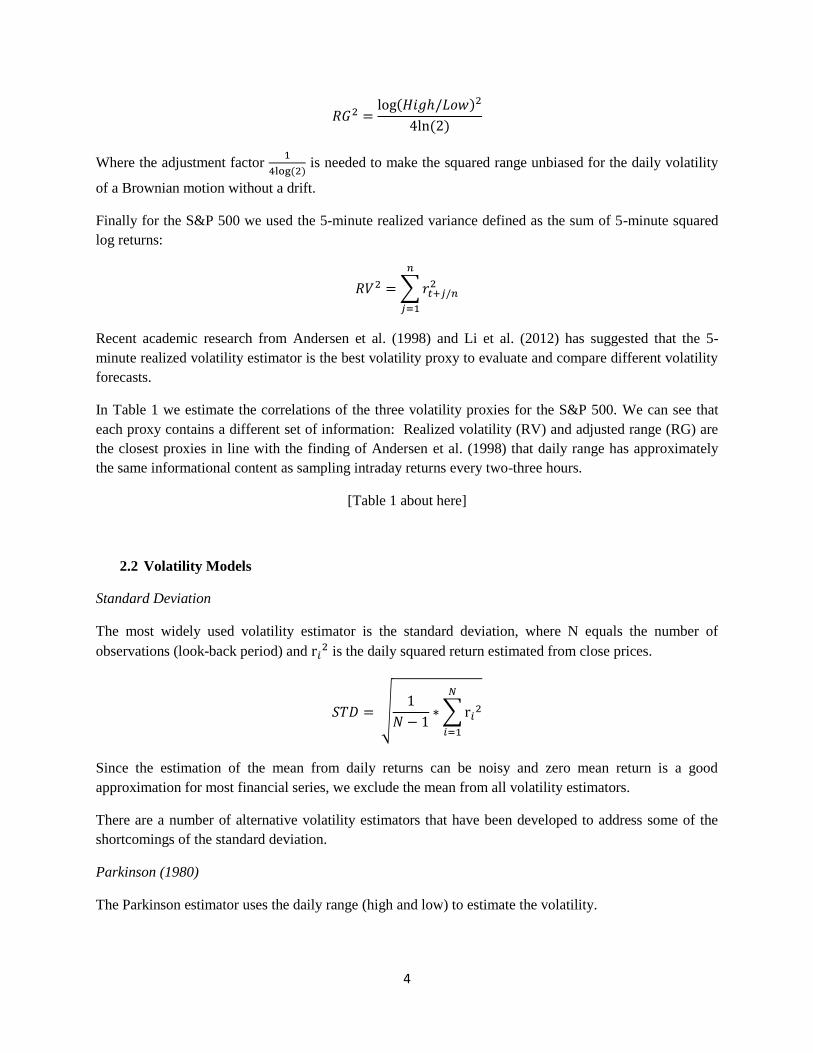
The adjusted squared daily range defined as:
4
( )
( )
Where the adjustment factor
( ) is needed to make the squared range unbiased for the daily volatility
of a Brownian motion without a drift.
Finally for the S&P 500 we used the 5-minute realized variance defined as the sum of 5-minute squared
log returns:
∑
Recent academic research from Andersen et al. (1998) and Li et al. (2012) has suggested that the 5-
minute realized volatility estimator is the best volatility proxy to evaluate and compare different volatility
forecasts.
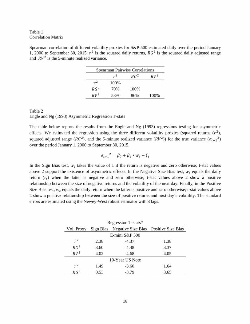
In Table 1 we estimate the correlations of the three volatility proxies for the S&P 500. We can see that
each proxy contains a different set of information: Realized volatility (RV) and adjusted range (RG) are
the closest proxies in line with the finding of Andersen et al. (1998) that daily range has approximately
the same informational content as sampling intraday returns every two-three hours.
[Table 1 about here]
2.2 Volatility Models
Standard Deviation
The most widely used volatility estimator is the standard deviation, where N equals the number of
observations (look-back period) and is the daily squared return estimated from close prices.
√
∑
Since the estimation of the mean from daily returns can be noisy and zero mean return is a good
approximation for most financial series, we exclude the mean from all volatility estimators.
There are a number of alternative volatility estimators that have been developed to address some of the
shortcomings of the standard deviation.
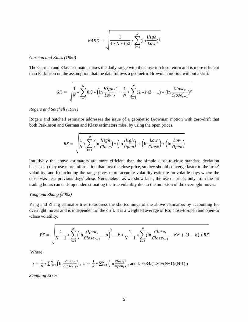
Parkinson (1980)
The Parkinson estimator uses the daily range (high and low) to estimate the volatility.
5
√
∑(
)
Garman and Klass (1980)
The Garman and Klass estimator mixes the daily range with the close-to-close return and is more efficient
than Parkinson on the assumption that the data follows a geometric Brownian motion without a drift.
√
∑ (
)
∑( ) (
)
Rogers and Satchell (1991)
Rogers and Satchell estimator addresses the issue of a geometric Brownian motion with zero-drift that
both Parkinson and Garman and Klass estimators miss, by using the open prices.
√
∑(
) (
)
(
) (
)
Intuitively the above estimators are more efficient than the simple close-to-close standard deviation
because a) they use more information than just the close price, so they should converge faster to the ‘true’
volatility, and b) including the range gives more accurate volatility estimate on volatile days where the
close was near previous days’ close. Nonetheless, as we show later, the use of prices only from the pit
trading hours can ends up underestimating the true volatility due to the omission of the overnight moves.
Yang and Zhang (2002)
Yang and Zhang estimator tries to address the shortcomings of the above estimators by accounting for
overnight moves and is independent of the drift. It is a weighted average of RS, close-to-open and open-to
-close volatility.
√
∑(
)
∑(
) ( )
Where
∑ (
)
,
∑ (
)
, and k=0.34/(1.34+(N+1)/(N-1) )
Sampling Error
6
All the estimators above have a look-back period which means that they are subject to sampling error. We
adjust for that by dividing the estimated volatility by the adjustment factor as shown by Sinclair (2008):
( ) √
( )
(
)
Where N is the sample size and Γ is the gamma function.
We divide our volatility estimates by the adjustment factor to get the ‘unbiased’ volatility that we use.
Although the above estimators are more efficient than the standard deviation by incorporating more
information, they do not incorporate empirical regularities of the financial times series. Specifically,
volatility of the financial time series exhibits some well-known effects: 1) it is time-varying, 2) it clusters
(squared and absolute returns exhibit high degree of autocorrelation which allows us to consider volatility
as almost stable in the short run), and 3) it tends to mean-revert.
Exponential Weighted Moving Average (EWMA)
The RiskMetrics (1996) approach is built upon the first two effects. Variance is modeled using an
exponential moving average (EWMA) where the estimate for time t is a weighted average of the previous
estimates. Symbolically this is:
( )
Where is the decay factor. The most recent observations receive higher weights and the weights on the
past observations decrease geometrically. The half-life of the number of days used in estimation can be
derived by the fraction ln(2)/ln( ). We will be using the same parameter that RiskMetrics recommends (
=0.94 which corresponds to 17-day half-life). The advantage of this model is its simplicity and easiness of
its estimation. Its main weaknesses are 1) it assumes that returns are iid and normally distributed, 2)
shocks persist forever, and 3) the volatility for tomorrow is today’s volatility.
GARCH
The GARCH model proposed by Engle (1982) and Bollerslev (1986) uses all 3 characteristics to model
the variance. It assumes that variance is time-varying exhibiting high degree of auto-correlation but
reverts back to its long-term average. The simplest GARCH (1,1) equation can be written as:
The ratio
( ) equals the long-term (unconditional) variance assuming that the model is
covariance stationary ( + <1). The sum + is the persistence term that controls for the speed of
mean reversion and the ratio of ln(0.5)/( + ) is the half-life of mean reversion that measures the
average time it takes for a shock - to decrease by half. If + >1 the GARCH model is non-
stationary and the volatility will eventually explode.
Asymmetric Volatility Effects
7
In some assets volatility tends to respond differently to the sign of past returns. For example in equities it
is well documented that volatility tends to increase more after big down days than big up days. We test for
asymmetric effects applying the regression tests used by Engle and Ng (1993).
Where is the daily volatility proxy squared and is a variable constructed from the daily return
( ) and its sign. More specifically, in the Sign Bias test it takes the value of 1 if the return is negative and
zero otherwise; in the Negative Size Bias test it takes the value of when the latter is negative and zero
otherwise; and in the Positive Size Bias test it takes the value of when the latter is positive and zero
otherwise. Table 2 reports the results.
[Table 2 about here]
There is clear evidence for asymmetric volatility effects in the S&P 500; the Sign Bias test shows
statistically significant results and the Negative Size Bias t-stats are higher in magnitude than the Positive
Size Bias ones. The results hold for all volatility proxies. On the contrary, the evidence for asymmetric
volatility effects on the 10-Year Note is mixed. The Sign Bias test is not statistically significant for both
volatility proxies, while the Negative Size Bias is higher in magnitude than the Positive Size Bias when
the squared return is used but not when the adjusted squared range is used. Bonds seem to respond
symmetrically to volatility shocks. Overall, there is strong evidence for asymmetric effects in the S&P
500 and so we would expect asymmetric models to perform better than symmetric ones, whereas there is
no evidence for asymmetric effects in US 10-Year Note and so we would expect symmetric models to be
a better fit.
To consider asymmetric effects in volatility estimation and forecasting we apply the two most well-
known asymmetric GARCH models: TARCH (or GJR-GARCH) and EGARCH.
Threshold ARCH (TARCH)
Threshold ARCH (Glosten et al. (1993)) captures the asymmetry in volatility by introducing a dummy
variable I(t) in the GARCH equation that takes the value of 1 if the previous return is below a certain
threshold (we use zero as our threshold). More specifically its variance equation is:
( ( ))
Where the ratio
( ) equals the long term variance and the ratio of ln(0.5)/( + + /2) is
the half-life of mean reversion. Negative (positive) values for indicate increase in volatility after
negative (positive) shocks.
Exponential GARCH (EGARCH)
Exponential GARCH (Nelson (1991)) models the log of the variance as:
( ) ( | | | | ) ( )
8
where and | | √ . Negative (positive) values for indicate increase in volatility
after negative (positive) shocks. The long term log variance equals
( ) .
The main advantage of the EGARCH model is that it models the logarithm of variance and so the
positivity of variance is automatically satisfied without requiring restrictions on the maximization of the
log likelihood function.
GARCH Criticism
GARCH models are non-linear which means that their parameter estimation depends on an optimization
routine that is sensitive to a) starting values, b) algorithm and software used, c) training period, d)
maximum likelihood function (usually the normal distribution) and e) number of parameters. Differences
in those specifications can result in different results. Furthermore, as Engle and Manganelli (2001)
mention, all GARCH-type models are subject to three different sources of misspecification: the variance
equation and the distribution chosen for the log-likelihood may be wrong and the standardized residuals
may not be identically and independently distributed (iid). Nevertheless, GARCH models appear to fit the
empirical data quite well and are used extensively in industry and academia.
2.3 VaR Methodologies
VaR measures the maximum expected loss over a certain horizon with a given probability. Since this
number depends on the confidence level we examine three different quantiles (1%, 5% and 10%) of both
sides of the distribution to get a better understanding of the tails. We look at two different methodologies
of VaR forecasting that are the most prevalent in the industry because of their relative computational
easiness and low complexity.
Parametric
The VaR computation can be simplified considerably if the distribution is assumed to belong to a
parametric family such as the normal distribution. This way VaR can be derived directly from the
volatility using a multiplicative factor that depends on the confidence level. In this paper we estimate the
parametric VaR by multiplying each conditional volatility estimation by the standardized normal
distribution quantiles.
Semi-Parametric: Quasi-Maximum Likelihood GARCH (QML GARCH)
According to Alexander (2008), VaR estimation using analytic GARCH ignores the purpose of GARCH
(volatility clustering after a market shock) because we assume away the possibility of a shock by simply
plugging in the GARCH volatility into a VaR formula. Also, using GARCH in a normal linear VaR is
wrong from a theoretical standpoint since the VaR analytic formula assumes that returns are normal
whereas GARCH assumes that they follow a normal GARCH process. In othe words, the use of GARCH
in the analytic normal linear VaR is not correct and introduces an approximation error.
Bollerslev and Woolridge (1992) showed that the maximization of the normal GARCH likelihood is able
to deliver consistent estimates, provided that the variance equation is correctly specified, even if the
9
standardized residuals are not normally distributed. Using that result, Engle and Manganelli (1999),
compute the VaR by first fitting a GARCH model and then multiplying the empirical quantile of the
standardized residuals by the square root of the estimated variance. We employ the same procedure using
all three GARCH models.
3. Forecast Evaluation
3.1 Volatility Forecast Evaluation
Loss Functions
We measure the predictive accuracy of each volatility estimator by the average forecast loss. The more
accurate the model, the lower its average loss should be. As Patton (2010) showed, apart from an accurate
volatility proxy, a robust loss function is required to compare different volatility forecasts in the sense that
they asymptotically generate the same ranking of models regardless of the proxy for the true volatility.
Following Patton (2010) we use the Quasi-Likelihood and Mean Squared Error loss functions.
Quasi-Likelihood Loss (QL)
∑
Root Mean Squared Error (RMSE)
√∑ (
)
Similar to Brownless et al. (2014) we prefer the QL loss function because 1) the loss series is iid under
the null hypothesis that the forecasting model is correctly specified, whereas MSE loss series exhibits
high degree of autocorrelation even under the null, and 2) MSE has a bias that depends on the level of
volatility whereas QL is independent of the level.
Pairwise Comparison of Volatility Forecasts
We use the Diebold-Mariano test (DM) to compare in a pairwise fashion the forecasts using the QL loss
function for the reasons explained above. The DM test tests the null hypothesis of equal predictive
accuracy against the alternative that a forecast is superior. Since true volatility is unobservable, the test is
implemented using a statistic based on the difference between QL losses measured using all different
volatility proxies. More specifically,
is the difference between the QL losses of A and B. Negative (Positive) d values mean that the forecast A
is less (more) accurate than forecast B. The DM test statistic is computed using a standardized t-test:
10
√ ( )
Where ∑
is the average difference between the QL losses and avar is a consistent estimate of the
variance of to account for the serial correlation of the loss differentials. We use the Newey-West
variance estimator as recommended by Dieblod et al. Under the null hypothesis the test statistic is
asymptotically normally distributed.
3.2 VaR Forecast Evaluation
We forecast VaR for three different quantiles: 1%, 5% and 10% for both tails of the distribution since we
consider the risk of both long and short positions. We place more emphasis on the 5th quantile because the
sample size of expected violations contains enough extreme observations to be used in statistical tests
boosting their power. We also closely examine the 1% quantile that contains important information about
the extreme tails of the distribution although it has a smaller number of expected violations. We evaluate
the VaR forecasts following the framework of Christoffersen (1998) designed for evaluating the accuracy
of out-of-sample interval forecasts.
Unconditional Coverage
Since VaR is reported at a specified confidence level (1-a%), we expect it to be exceeded a% of times in
the backtest. Of course, we cannot expect the % of exceptions to match exactly a% since there is
randomness. To test whether the exceptions are a result of randomness or of a systematic bias in our
methodology, we use the non-parametric Bernouli trials test. Under the null hypothesis that VaR is
correctly estimated, the number of exceptions x of a sample size N, follows a binominal probability
distribution:
( ) ( ) ( )
Since our backtest sample is large, according to the central limit theorem, we can approximate the
binominal distribution by the normal distribution and estimate the z-score of the number of exceptions as:
( )
At 95% confidence level we would expect to see the z-score lying between -1.96 and 1.96. Values higher
(lower) than the cutoff value of 1.96 (-1.96) lead us to reject the null hypothesis that our VaR model is
unbiased and indicate systematic underestimation (overestimation) of risk. We also look at the upside and
downside VaR exceptions separately since a good VaR model should be directionally unbiased expecting
similar number of exceptions from both sides.
The above test is equivalent to the log-likelihood test:
( ) ( ) ( )
11
Which is asymptotically distributed chi-squared with one degree of freedom under the null hypothesis that
p is the true probability. At 95% confidence level values of LRuc>3.84 lead to rejection of the null.
Independence
The unconditional coverage test compares the overall number of VaR violations with the expected
number of violations ignoring the time variation in the data. In other words, it tells us nothing about how
close the violations are and if there is any clustering. Theoretically, violations should be spread evenly
over time.
To test the hypothesis that the forecast is accurate and that there is no clustering in violations we employ
Christoffersen’s (1998) independence test. The independence test statistic (LRind) tests for clustering in
violations modeling them as a binary first-order Markov chain with transition matrix:
[
]
Where is the probability of a violation after a day without a violation, whereas is the probability
of a violation after observing a violation the previous day. We estimate the probabilities by counting the
days where we had a violation conditional on the previous day. More specifically, is the number of
days where there was no violation following a no-violation day, is the number of days where there
was a violation following a no-violation day, is the number of days without violation following a
violation, and is the number of days with a violation following a violation.
The test statistic conditional on the first observation is:
[ ( )( )( )] ( )
( )
The likelihood ratio test is also asymptotically distributed chi-squared with one degree of freedom under
the null hypothesis of independence. At 95% confidence level values of LRind>3.84 lead to rejection of
the null.
The unconditional coverage and the independence properties are separate and distinct and must both be
satisfied by an accurate VaR model. In other words, we want the sequence of VaR violations to be
identically and independently distributed as a Bernoulli random variable. Thus, we will be looking for
models that pass both tests.
Finally, we evaluate the effectiveness of the VaR methods looking at the magnitude of the exceptions. In
other words, how wrong was our estimation when the VaR threshold was crossed. We estimate the
violation ratios as
| |
Where is our VaR estimate for a given confidence interval. For example, a ratio of 1.5 means that
the violation was 50% higher than our VaR estimate. We report the median, 90th percentile and max
(worst) violation ratios.
12
4. Empirical Results
4.1 Data and Estimation
Our dataset covers the period January 1, 2000 to September 30, 2015, with daily prices for E-mini S&P
500 and 10-Year US Note futures coming from Morningstar LIM. Since the GARCH models require a
long training sample, we start all our out-of-sample comparisons from January 2004, allowing enough
time for the GARCH models to be estimated. In all calculations we are using log prices and returns. The
Implied Volatility of S&P 500 is the VIX index whereas the Implied Volatility of the 10-Year US Note is
the TYVIX. Both indexes come from CBOE and are estimated under the same model-free methodology.
At the end of each day, we generate one day-ahead volatility forecast using each model with its pre-
specified look-back and training period and we compare it to next day’s volatility proxy. We follow the
same process for VaR forecasts using the volatility forecast and the relevant quantile. More specifically,
we estimate the following models using the selected parameters, look-backs and training periods that are
mostly used and cited in the industry and academic research.
Standard Deviation: Rolling over the last 30 days (STD_30)
Range-Based Volatility
1. Parkinson: Rolling window over the last 30 days (PARK_30)
2. Garman & Klass: Rolling window over the last 30 days (GK_30)
3. Roger & Satchell : Rolling window over the last 30 days (RS_30)
4. Yang & Zhang: Rolling window over the last 30 days (YZ_30)
GARCH Volatility
1. Exponential Moving Average using the RiskMetrics lambda=0.94 (EWMA)
2. GARCH(1,1): Estimated using an expanding window (GARCH)
3. GARCH(1,1): Rolling 1,000 observations window (GARCH-R)
4. TARCH(1,1,1): Estimated using an expanding window (TARCH)
5. EGARCH(1,1,1): Estimated using an expanding window (EGARCH)
Implied Volatility: VIX and TYVIX value of the previous day divided by (IV)
4.2 Descriptive Statistics
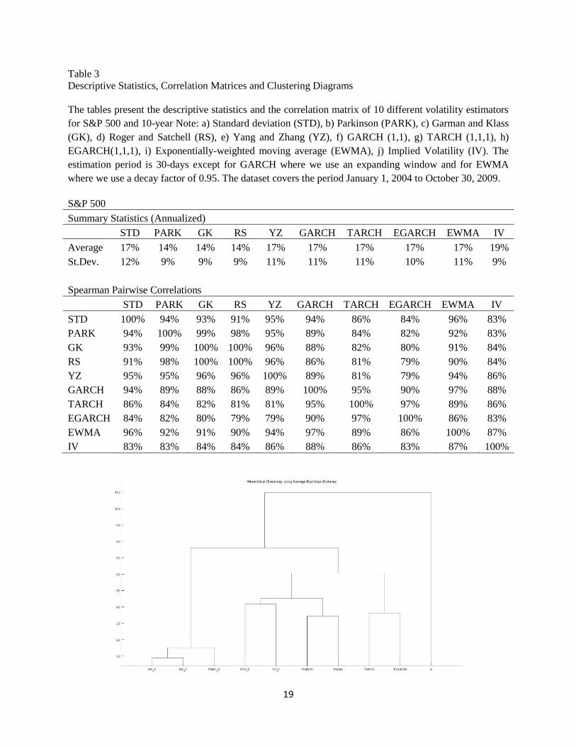
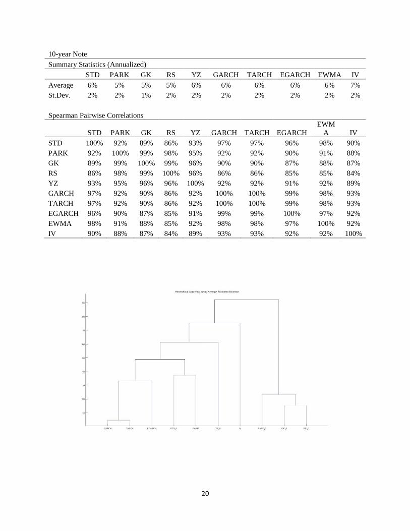
Table 3 reports the descriptive statistics for the volatility estimators used. We see that Implied Volatility
(IV) is biased higher than the rest of the volatility estimators because of its volatility premium. On the
contrary, range-based estimators are biased lower, mainly because of the omission of the overnight move.
All volatility estimators are highly correlated with the average pairwise correlation 89% in SP and 92% in
the 10-Year. Nevertheless, there is evidence that different volatility estimators contain different pieces of
information. More specifically, there are clusters created depending on the data that each estimator uses:
a) Range-based estimators (RARK, RS, GK) are highly correlated and constitute a separate cluster while
the YZ is between range-based and close-to-close estimators, b) Implied Volatility has the lowest average
correlation with the rest of volatility estimators and forms a cluster on its own. This was expected since it
contains an insurance premium and is forward-looking whereas the rest of the estimators are historical. c)
13
Close-to-Close estimators (STD, EWMA and GARCH models) form another cluster with GARCH
models constituting a sub-cluster, and d) for the S&P 500, the asymmetric GARCH models form another
sub-cluster.
[Table 3 about here]
4.3 Volatility Forecasting Results
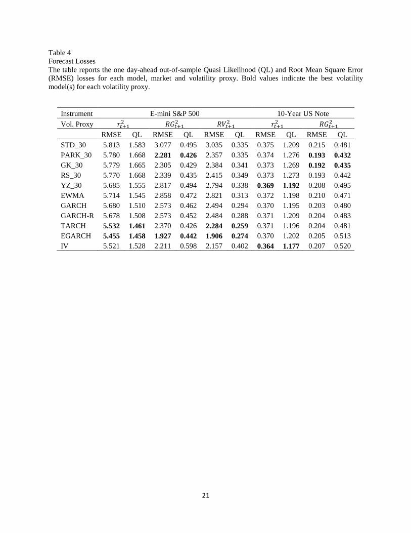
We evaluate the volatility forecasts by assessing the out-of-sample volatility forecast losses. Table 4
summarizes the forecasting results for each model using both the QL and the RMSE loss functions with
squared returns ( ), adjusted range (
) and realized volatility ( ) as a volatility proxies. We can
see that QL and MSE losses based on RV and RG are smaller than those based on for both S&P 500
and 10-Year Note due to the improved efficiency of both volatility proxies over the squared returns. Also,
the volatility of the 10-Year Note appears to be more forecastable than that of the S&P 500 producing
smaller QL losses for each estimator. The choices of loss function and volatility proxy do not change the
rankings substantially, but there is a tendency for GARCH models to perform better when the squared
return and realized variance are used as proxies, whereas range-based models perform better when the
adjusted range is used. Also, range-based models on average generate lower forecasting errors than the
standard deviation while GARCH models systematically outperform the other two close-to-close
volatility estimators (STD and EWMA). Regarding GARCH models, it appears that the use of an
expanding window instead of a rolling window produces more accurate forecasts and the asymmetric
versions are better in equities capturing the leverage effect, but they do not improve the symmetric ones in
the 10-Year Note.
[Table 4 about here]
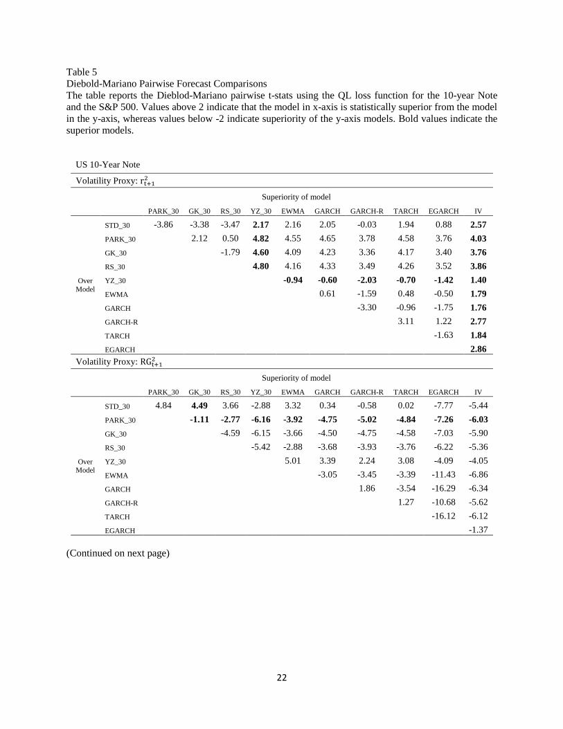
We also estimate the Diebold-Mariano pairwise statistics and report the results in Table 5. The results
confirm that the TARCH model is superior from the rest in the S&P 500 irrespective of the volatility
proxy that is being used. On the contrary, the results are mixed for the 10-Year depending on the volatility
proxy. Implied Volatility and YZ_30 appear to deliver superior forecasts under the squared return proxy,
whereas Parkinson ranks first when the adjusted range is used.
[Table 5 about here]
4.4 VaR Backtesting Results
In a similar fashion, we estimate the out-of-sample one day-ahead VaR forecasts under the parametric
approach multiplying the volatility forecast by the normal quantile. We also estimate the QML-GARCH
models by multiplying the empirical quantiles after fitting a GARCH model with the GARCH volatility
forecasts. For space reasons we do not report the results from the Garman & Klass (GK) and Roger &
Satchell (RS) estimators since their results are identical with the Parkinson estimator. We also exclude the
rolling GARCH since we showed that its forecasting power is weaker compared to GARCH estimated
14
over an expanding window. We examine three different quantiles 1%, 5% and 10% and we report the
percentage of exceptions of each model, their statistical significance along with the violation ratios and P-
values of the independence test in Table 6.
[Table 6 about here]
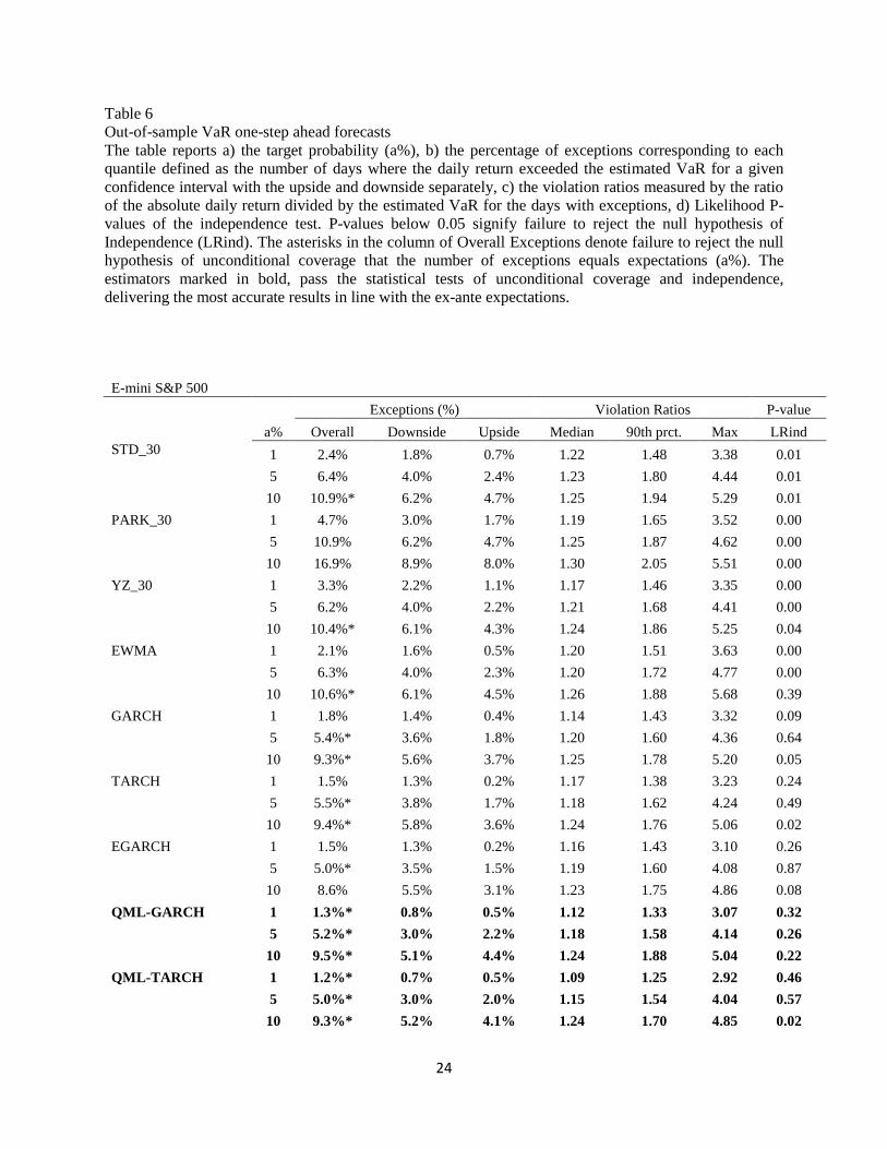
For the S&P 500, we can see that all models have more downside exceptions (when the stock index is
down) than upside. This shows that the distribution is not symmetric with the left tail fatter and the right
tail thinner. As a result, any volatility forecast based on analytic VaR with normal quantiles will fail,
underestimating the left tail and overestimating the right tail. This does not mean that the volatility
forecast is bad, but that the distribution is not correctly specified. Parkinson estimator is biased
downwards because it ignores the overnight move leading to systematic risk underestimation. The result
(not reported here) holds for the rest of range-based estimators. On the other hand, implied volatility
produces upwards biased VaR forecasts due to the volatility premium, making it a bad risk indicator. The
superiority of GARCH models in volatility forecasting is evident when we compare their VaR forecasts
based on the normal quantiles with the rest of the models. They offer the best parametric VaR forecasts
passing the tests of unconditional coverage and independence, failing only at the 1% quantile. This shows
that a more accurate volatility forecast can produce a superior and adequate VaR forecast, except for the
lower tail, even if the distribution is mis-specified. QML-GARCH models, and specifically QML-
GARCH and QML-TARCH, fill that gap offering the most accurate VaR forecasts beating all other
models and methods. The combination of superior volatility forecast from the GARCH models with the
estimation of the empirical quantile that allows them to incorporate distributional asymmetries delivers
robust and unbiased results for all quantiles passing all statistical tests at all quantiles.
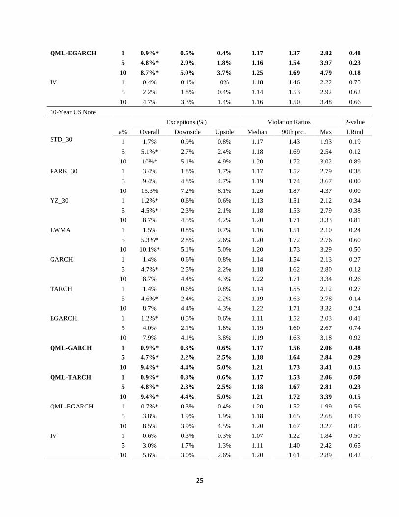
In contrast with the S&P 500, the results for the 10-Year Note show that most of the estimators do an
adequate job in estimating risk. This is a result of a) higher forecastability of bond volatility, and b) more
symmetric distribution of bond returns. More specifically, EWMA and STD produce good VaR forecasts
for the 5% and 10% quantiles passing the tests of unconditional coverage and independence, failing only
at the 1% quantile. Yang-Zhang (YZ) does a remarkable job at the lowest quantiles (1% and 5%) and is
slightly biased higher at the 10% quantile, passing all the tests of unconditional coverage and
independence for all quantiles. On the other hand, Parkinson, again, underestimates risk, whereas Implied
Volatility systematically overestimates it. In contrast with the S&P 500 results, GARCH models do not
generate superior VaR forecasts from the rest of the models having a tendency to underestimate VaR at
the lowest quantile and overestimate it at the 10% quantile. However, QML-GARCH models and
specifically QML-GARCH and QML-TARCH, deliver, again, superior results passing all the statistical
tests at all quantiles and outperforming the rest of the models and methods. This result shows how
important is the flexibility to fit the empirical distribution.
5. Conclusion
Volatility forecasting has paramount importance in position sizing and risk management of CTAs. In this
paper we take a pragmatic approach and compare different volatility estimators that are widely used in
industry and academia, examining their one-day ahead out-of-sample forecasts from a statistical and
Value-at-Risk perspective.
15
Although we do not find evidence for a volatility estimator that is statistically superior in the assets we
study, we show that asymmetric GARCH models (TARCH and EGARCH) generate superior forecasts for
the S&P 500, whereas symmetric models such as GARCH, Yang-Zhang along with the implied volatility
perform better in the 10-Year Note. In other words, the volatility process of each asset can differ and a
good volatility estimator should incorporate the empirical regularities related to each asset. We also find
evidence that the volatility of the 10-Year Note is more forecastable than that of the S&P 500 producing
smaller errors.
Furthermore, we show that improving the volatility forecast can generate superior VaR forecasts that can
be accurate under the normal distribution failing the tests only at the lowest quantile. More specifically,
GARCH models produce superior forecasts failing only at the 1% quantile. More importantly we show
that the reason that most models fail is mainly because the distribution is mispecified and badly
approximated by the normal. Finally, we show that the semi-parametric QML-GARCH models that use
the empirical quantiles of the distribution along with GARCH volatility forecast address that issue and
generate superior VaR forecasts outperforming all other methods in all quantiles.
References
Alexander, C. (2001), Market Risk Analysis Volume II: Practical Financial Econometrics, Wiley,
London.
Andersen, T.G. and Bollerslev, T. (1998a), Answering the skeptics: Yes, standard volatility models do
provide accurate forecasts, International Economic Review 39, 885–905.
Andersen, T. G., Bollerslev, T., Christoffersen, P. F., and Diebold, F. X. (2006), Volatility and correlation
forecasting. In Handbook of Economic Forecasting, Elliott, G., Granger, C. W. J., and Timmermann, A.
(eds). North-Holland, Amsterdam.
Baltas, A. N. and Kosowski, R. (2013), Improving time-series momentum strategies: the role of volatility
estimators and trading signals, SSRN eLibrary.
Bollerslev, T. (1986), Generalized autoregressive conditional heteroskedasticity, Journal of Econometrics
31, 307–327.
Bollerslev, T. and Wooldridge, J.M. (1992), Quasi-maximum likelihood estimation and inference in
dynamic models with time varying covariances, Econometric Reviews 11, 143–172.
Brandt, M. W. and Kinlay, J. (2005), Estimating historical volatility, Research Article, Investment
Analytics
Brownlees, C., Engle, R., and Kelly, B. (2011), A practical guide to volatility forecasting through calm
and storm, (Appendix) Technical Report. URL: http://pages.stern.nyu.edu/ ˜ cbrownle.
Christoffersen, P.F. (1998), Evaluating interval forecasts, International Economic Review 39, 841–862.
16
Christoffersen, P.F., Hahn, J., Inoue, A. (2001), Testing and comparing value-at-risk measures. Journal of
Empirical Finance 8, 325–342.
Christoffersen, P.F. and Pelletier, D. (2004), Backtesting value-at-risk: A duration-based approach,
Journal of Financial Econometrics 2, 84–108.
Diebold, F.X. and Mariano, R.S. (1995), Comparing predictive accuracy, Journal of Business and
Economic Statistics 13, 253–265.
DeSantis, G., Litterman, R., Vesval, A., Winkelmann, K. (2003), Covariance matrix estimation, In:
Litterman, R. (Ed.), Modern Investment Management: An Equilibrium Approach, Wiley, London.
Engle, R. F. (1982), Autoregressive conditional heteroscedasticity with estimates of the variance of
United Kingdom inflation, Econometrica 50(4), 987–1007.
Engle, R. F., Ng V. (1993), Measuring and Testing the Impact of News on Volatility, Journal of Finance,
December, 48:5, pp. 1749-78.
Fleming, J., Kirby, C., Ostdiek, B. (2003), The economic value of volatility timing using “realized”
volatility, Journal of Financial Economics 67, 473–509.
Garman, M. B., and Klass M. J. (1980), On the Estimation of Security Price Volatilities from Historical
Data, Journal of Business 53, pp. 67-78.
Glosten, L. R., Jagannanthan, R., and Runkle, D. E. (1993), On the relation between the expected value
and the volatility of the nominal excess return on stocks, Journal of Finance 48(5), 1779–1801.
Hansen, P. R., and Lunde, A. (2005b), Consistent ranking of volatility models, Journal of Econometrics
131(1), 97–121.
Hallerbach, W. G. (2012), A Proof of the Optimality of Volatility Weighting Over Time. Available at
SSRN: http://ssrn.com/abstract=2008176 or http://dx.doi.org/10.2139/ssrn.2008176
J.P. Morgan (1996), RiskMetrics, Technical Documents, fourth ed., New York.
Liu, L. and Patton, A. and Sheppard, K. (2012), Does Anything Beat 5-Minute RV? A Comparison of
Realized Measures Across Multiple Asset Classes. Available at SSRN: http://ssrn.com/abstract=2214997
or http://dx.doi.org/10.2139/ssrn.2214997.
Manganelli , S. and Engle, R. F. (2001), Value at Risk Models in Finance, ECB Working Paper No. 75.
Available at SSRN: http://ssrn.com/abstract=356220
Nelson, D. B. (1991), Conditional heteroskedasticity in asset returns: a new approach, Econometrica
59(2), 347–370.
Newey, W. K. and West, K. D. (1987), A simple, positive semi-definite, heteroskedasticity and
autocorrelation consistent covariance matrix, Econometrica 55(3), 703–708.
17
Patton, A. (2009), Volatility forecast comparison using imperfect volatility proxies, Technical Report,
University of Oxford.
Parkinson, M. (1980), The extreme value method for estimating the variance of the rate of returns, Journal
of Business 53, 61–65.
Rogers, L. C. G., and S. E. Satchell (1991), Estimating Variance from High, Low and Closing Prices,
Annals of Applied Probability 1, pp. 504-512.
Sinclair, E. (2013), Volatility Trading, Wiley.
Yang, D., and Q. Zhang (2000), Drift Independent Volatility Estimation Based on High, Low, Open, and
Close Prices, Journal of Business 73, pp. 477-492.
18
Table 1
Correlation Matrix
Spearman correlation of different volatility proxies for S&P 500 estimated daily over the period January
1, 2000 to September 30, 2015. is the squared daily returns, is the squared daily adjusted range
and is the 5-minute realized variance.
Spearman Pairwise Correlations
100%
70% 100%
53% 86% 100%
Table 2
Engle and Ng (1993) Asymmetric Regression T-stats
The table below reports the results from the Engle and Ng (1993) regressions testing for asymmetric
effects. We estimated the regression using the three different volatility proxies (squared returns ( ),
squared adjusted range ( ), and the 5-minute realized variance ( )) for the true variance ( )
over the period January 1, 2000 to September 30, 2015.
In the Sign Bias test, takes the value of 1 if the return is negative and zero otherwise; t-stat values
above 2 support the existence of asymmetric effects. In the Negative Size Bias test, equals the daily
return ( ) when the latter is negative and zero otherwise; t-stat values above 2 show a positive
relationship between the size of negative returns and the volatility of the next day. Finally, in the Positive
Size Bias test, equals the daily return when the latter is positive and zero otherwise; t-stat values above
2 show a positive relationship between the size of positive returns and next day’s volatility. The standard
errors are estimated using the Newey-West robust estimator with 8 lags.
Regression T-stats*
Vol. Proxy Sign Bias Negative Size Bias Positive Size Bias
E-mini S&P 500
2.38 -4.37 1.38
3.60 -4.48 3.37
4.02 -4.68 4.05
10-Year US Note
1.49 -3.60 1.64
0.53 -3.79 3.65
19
Table 3
Descriptive Statistics, Correlation Matrices and Clustering Diagrams
The tables present the descriptive statistics and the correlation matrix of 10 different volatility estimators
for S&P 500 and 10-year Note: a) Standard deviation (STD), b) Parkinson (PARK), c) Garman and Klass
(GK), d) Roger and Satchell (RS), e) Yang and Zhang (YZ), f) GARCH (1,1), g) TARCH (1,1,1), h)
EGARCH(1,1,1), i) Exponentially-weighted moving average (EWMA), j) Implied Volatility (IV). The
estimation period is 30-days except for GARCH where we use an expanding window and for EWMA
where we use a decay factor of 0.95. The dataset covers the period January 1, 2004 to October 30, 2009.
S&P 500
Summary Statistics (Annualized)
STD PARK GK RS YZ GARCH TARCH EGARCH EWMA IV
Average 17% 14% 14% 14% 17% 17% 17% 17% 17% 19%
St.Dev. 12% 9% 9% 9% 11% 11% 11% 10% 11% 9%
Spearman Pairwise Correlations
STD PARK GK RS YZ GARCH TARCH EGARCH EWMA IV
STD 100% 94% 93% 91% 95% 94% 86% 84% 96% 83%
PARK 94% 100% 99% 98% 95% 89% 84% 82% 92% 83%
GK 93% 99% 100% 100% 96% 88% 82% 80% 91% 84%
RS 91% 98% 100% 100% 96% 86% 81% 79% 90% 84%
YZ 95% 95% 96% 96% 100% 89% 81% 79% 94% 86%
GARCH 94% 89% 88% 86% 89% 100% 95% 90% 97% 88%
TARCH 86% 84% 82% 81% 81% 95% 100% 97% 89% 86%
EGARCH 84% 82% 80% 79% 79% 90% 97% 100% 86% 83%
EWMA 96% 92% 91% 90% 94% 97% 89% 86% 100% 87%
IV 83% 83% 84% 84% 86% 88% 86% 83% 87% 100%
20
10-year Note
Summary Statistics (Annualized)
STD PARK GK RS YZ GARCH TARCH EGARCH EWMA IV
Average 6% 5% 5% 5% 6% 6% 6% 6% 6% 7%
St.Dev. 2% 2% 1% 2% 2% 2% 2% 2% 2% 2%
Spearman Pairwise Correlations
STD PARK GK RS YZ GARCH TARCH EGARCH
EWM
A IV
STD 100% 92% 89% 86% 93% 97% 97% 96% 98% 90%
PARK 92% 100% 99% 98% 95% 92% 92% 90% 91% 88%
GK 89% 99% 100% 99% 96% 90% 90% 87% 88% 87%
RS 86% 98% 99% 100% 96% 86% 86% 85% 85% 84%
YZ 93% 95% 96% 96% 100% 92% 92% 91% 92% 89%
GARCH 97% 92% 90% 86% 92% 100% 100% 99% 98% 93%
TARCH 97% 92% 90% 86% 92% 100% 100% 99% 98% 93%
EGARCH 96% 90% 87% 85% 91% 99% 99% 100% 97% 92%
EWMA 98% 91% 88% 85% 92% 98% 98% 97% 100% 92%
IV 90% 88% 87% 84% 89% 93% 93% 92% 92% 100%
21
Table 4
Forecast Losses
The table reports the one day-ahead out-of-sample Quasi Likelihood (QL) and Root Mean Square Error
(RMSE) losses for each model, market and volatility proxy. Bold values indicate the best volatility
model(s) for each volatility proxy.
Instrument E-mini S&P 500 10-Year US Note
Vol. Proxy
RMSE QL RMSE QL RMSE QL RMSE QL RMSE QL
STD_30 5.813 1.583 3.077 0.495 3.035 0.335 0.375 1.209 0.215 0.481
PARK_30 5.780 1.668 2.281 0.426 2.357 0.335 0.374 1.276 0.193 0.432
GK_30 5.779 1.665 2.305 0.429 2.384 0.341 0.373 1.269 0.192 0.435
RS_30 5.770 1.668 2.339 0.435 2.415 0.349 0.373 1.273 0.193 0.442
YZ_30 5.685 1.555 2.817 0.494 2.794 0.338 0.369 1.192 0.208 0.495
EWMA 5.714 1.545 2.858 0.472 2.821 0.313 0.372 1.198 0.210 0.471
GARCH 5.680 1.510 2.573 0.462 2.494 0.294 0.370 1.195 0.203 0.480
GARCH-R 5.678 1.508 2.573 0.452 2.484 0.288 0.371 1.209 0.204 0.483
TARCH 5.532 1.461 2.370 0.426 2.284 0.259 0.371 1.196 0.204 0.481
EGARCH 5.455 1.458 1.927 0.442 1.906 0.274 0.370 1.202 0.205 0.513
IV 5.521 1.528 2.211 0.598 2.157 0.402 0.364 1.177 0.207 0.520
22
Table 5
Diebold-Mariano Pairwise Forecast Comparisons
The table reports the Dieblod-Mariano pairwise t-stats using the QL loss function for the 10-year Note
and the S&P 500. Values above 2 indicate that the model in x-axis is statistically superior from the model
in the y-axis, whereas values below -2 indicate superiority of the y-axis models. Bold values indicate the
superior models.
US 10-Year Note
Volatility Proxy:
Superiority of model
PARK_30 GK_30 RS_30 YZ_30 EWMA GARCH GARCH-R TARCH EGARCH IV
Over
Model
STD_30 -3.86 -3.38 -3.47 2.17 2.16 2.05 -0.03 1.94 0.88 2.57
PARK_30 2.12 0.50 4.82 4.55 4.65 3.78 4.58 3.76 4.03
GK_30 -1.79 4.60 4.09 4.23 3.36 4.17 3.40 3.76
RS_30 4.80 4.16 4.33 3.49 4.26 3.52 3.86
YZ_30 -0.94 -0.60 -2.03 -0.70 -1.42 1.40
EWMA 0.61 -1.59 0.48 -0.50 1.79
GARCH -3.30 -0.96 -1.75 1.76
GARCH-R 3.11 1.22 2.77
TARCH -1.63 1.84
EGARCH 2.86
Volatility Proxy:
Superiority of model
PARK_30 GK_30 RS_30 YZ_30 EWMA GARCH GARCH-R TARCH EGARCH IV
Over Model
STD_30 4.84 4.49 3.66 -2.88 3.32 0.34 -0.58 0.02 -7.77 -5.44
PARK_30 -1.11 -2.77 -6.16 -3.92 -4.75 -5.02 -4.84 -7.26 -6.03
GK_30 -4.59 -6.15 -3.66 -4.50 -4.75 -4.58 -7.03 -5.90
RS_30 -5.42 -2.88 -3.68 -3.93 -3.76 -6.22 -5.36
YZ_30 5.01 3.39 2.24 3.08 -4.09 -4.05
EWMA -3.05 -3.45 -3.39 -11.43 -6.86
GARCH 1.86 -3.54 -16.29 -6.34
GARCH-R 1.27 -10.68 -5.62
TARCH -16.12 -6.12
EGARCH -1.37
(Continued on next page)

23
(Continued from previous page)
E-mini S&P 500
Volatility Proxy:
Superiority of model
PARK_30 GK_30 RS_30 YZ_30 EWMA GARCH GARCH-R TARCH EGARCH IV
Over Model
STD_30 -3.89 -3.57 -3.65 3.09 4.35 6.21 4.96 7.9 7.14 2.03
PARK_30 0.97 -0.12 5.42 5.22 5.34 5.05 6.26 6.04 3.25
GK_30 1.25 5.26 4.96 5.12 4.86 6.03 5.84 3.15
RS_30 5.41 5.1 5.2 4.93 6.1 5.9 3.21
YZ_30 0.94 3.39 2.92 5.43 5.06 0.95
EWMA 3.16 2.46 5.57 4.85 0.54
GARCH 0.4 6.99 4.9 -1.11
GARCH-R 5.51 4.35 -1.35
TARCH 0.35 -3.9
EGARCH -4.19
Volatility Proxy:
Superiority of model
PARK_30 GK_30 RS_30 YZ_30 EWMA GARCH GARCH-R TARCH EGARCH IV
Over
Model
STD_30 5.33 5 4.21 0.33 4.76 4.81 5.09 7.54 5.56 -8.61
PARK_30 -2.02 -3.59 -6.17 -3.06 -2.04 -1.39 -0.05 -0.82 -7.57
GK_30 -3.96 -5.9 -2.84 -1.85 -1.21 0.13 -0.64 -7.45
RS_30 -4.95 -2.28 -1.43 -0.85 0.42 -0.32 -6.9
YZ_30 3.32 3.5 3.98 5.96 4.44 -7.94
EWMA 1.79 2.85 6.12 3.61 -11.84
GARCH 3.88 9.69 4.14 -18.33
GARCH-R 6.49 1.98 -21.1
TARCH -5.59 -25.17
EGARCH -22.12
Volatility Proxy:
Superiority of model
PARK_30 GK_30 RS_30 YZ_30 EWMA GARCH GARCH-R TARCH EGARCH IV
Over Model
STD_30 -0.05 -0.37 -0.78 -0.67 5.45 4.81 4.36 6.44 4.93 -5.27
PARK_30 -2.86 -4.13 -0.24 1.3 1.62 1.73 2.67 2.13 -2.32
GK_30 -5.35 0.22 1.54 1.77 1.87 2.76 2.24 -2.02
RS_30 0.76 1.9 2.02 2.1 2.95 2.45 -1.68
YZ_30 4.46 3.39 3.33 4.85 3.85 -3.8
EWMA 2 2.14 4.25 2.95 -6.45
GARCH 2.05 8.29 3.85 -16.99
GARCH-R 7.03 2.81 -19.41
TARCH -5.74 -27.07
EGARCH -23.67
24
Table 6
Out-of-sample VaR one-step ahead forecasts
The table reports a) the target probability (a%), b) the percentage of exceptions corresponding to each
quantile defined as the number of days where the daily return exceeded the estimated VaR for a given
confidence interval with the upside and downside separately, c) the violation ratios measured by the ratio
of the absolute daily return divided by the estimated VaR for the days with exceptions, d) Likelihood P-
values of the independence test. P-values below 0.05 signify failure to reject the null hypothesis of
Independence (LRind). The asterisks in the column of Overall Exceptions denote failure to reject the null
hypothesis of unconditional coverage that the number of exceptions equals expectations (a%). The
estimators marked in bold, pass the statistical tests of unconditional coverage and independence,
delivering the most accurate results in line with the ex-ante expectations.
E-mini S&P 500
Exceptions (%) Violation Ratios P-value
a% Overall Downside Upside Median 90th prct. Max LRind
STD_30 1 2.4% 1.8% 0.7% 1.22 1.48 3.38 0.01
5 6.4% 4.0% 2.4% 1.23 1.80 4.44 0.01
10 10.9%* 6.2% 4.7% 1.25 1.94 5.29 0.01
PARK_30 1 4.7% 3.0% 1.7% 1.19 1.65 3.52 0.00
5 10.9% 6.2% 4.7% 1.25 1.87 4.62 0.00
10 16.9% 8.9% 8.0% 1.30 2.05 5.51 0.00
YZ_30 1 3.3% 2.2% 1.1% 1.17 1.46 3.35 0.00
5 6.2% 4.0% 2.2% 1.21 1.68 4.41 0.00
10 10.4%* 6.1% 4.3% 1.24 1.86 5.25 0.04
EWMA 1 2.1% 1.6% 0.5% 1.20 1.51 3.63 0.00
5 6.3% 4.0% 2.3% 1.20 1.72 4.77 0.00
10 10.6%* 6.1% 4.5% 1.26 1.88 5.68 0.39
GARCH 1 1.8% 1.4% 0.4% 1.14 1.43 3.32 0.09
5 5.4%* 3.6% 1.8% 1.20 1.60 4.36 0.64
10 9.3%* 5.6% 3.7% 1.25 1.78 5.20 0.05
TARCH 1 1.5% 1.3% 0.2% 1.17 1.38 3.23 0.24
5 5.5%* 3.8% 1.7% 1.18 1.62 4.24 0.49
10 9.4%* 5.8% 3.6% 1.24 1.76 5.06 0.02
EGARCH 1 1.5% 1.3% 0.2% 1.16 1.43 3.10 0.26
5 5.0%* 3.5% 1.5% 1.19 1.60 4.08 0.87
10 8.6% 5.5% 3.1% 1.23 1.75 4.86 0.08
QML-GARCH 1 1.3%* 0.8% 0.5% 1.12 1.33 3.07 0.32
5 5.2%* 3.0% 2.2% 1.18 1.58 4.14 0.26
10 9.5%* 5.1% 4.4% 1.24 1.88 5.04 0.22
QML-TARCH 1 1.2%* 0.7% 0.5% 1.09 1.25 2.92 0.46
5 5.0%* 3.0% 2.0% 1.15 1.54 4.04 0.57
10 9.3%* 5.2% 4.1% 1.24 1.70 4.85 0.02
25
QML-EGARCH 1 0.9%* 0.5% 0.4% 1.17 1.37 2.82 0.48
5 4.8%* 2.9% 1.8% 1.16 1.54 3.97 0.23
10 8.7%* 5.0% 3.7% 1.25 1.69 4.79 0.18
IV 1 0.4% 0.4% 0% 1.18 1.46 2.22 0.75
5 2.2% 1.8% 0.4% 1.14 1.53 2.92 0.62
10 4.7% 3.3% 1.4% 1.16 1.50 3.48 0.66
10-Year US Note
Exceptions (%) Violation Ratios P-value
a% Overall Downside Upside Median 90th prct. Max LRind
STD_30 1 1.7% 0.9% 0.8% 1.17 1.43 1.93 0.19
5 5.1%* 2.7% 2.4% 1.18 1.69 2.54 0.12
10 10%* 5.1% 4.9% 1.20 1.72 3.02 0.89
PARK_30 1 3.4% 1.8% 1.7% 1.17 1.52 2.79 0.38
5 9.4% 4.8% 4.7% 1.19 1.74 3.67 0.00
10 15.3% 7.2% 8.1% 1.26 1.87 4.37 0.00
YZ_30 1 1.2%* 0.6% 0.6% 1.13 1.51 2.12 0.34
5 4.5%* 2.3% 2.1% 1.18 1.53 2.79 0.38
10 8.7% 4.5% 4.2% 1.20 1.71 3.33 0.81
EWMA 1 1.5% 0.8% 0.7% 1.16 1.51 2.10 0.24
5 5.3%* 2.8% 2.6% 1.20 1.72 2.76 0.60
10 10.1%* 5.1% 5.0% 1.20 1.73 3.29 0.50
GARCH 1 1.4% 0.6% 0.8% 1.14 1.54 2.13 0.27
5 4.7%* 2.5% 2.2% 1.18 1.62 2.80 0.12
10 8.7% 4.4% 4.3% 1.22 1.71 3.34 0.26
TARCH 1 1.4% 0.6% 0.8% 1.14 1.55 2.12 0.27
5 4.6%* 2.4% 2.2% 1.19 1.63 2.78 0.14
10 8.7% 4.4% 4.3% 1.22 1.71 3.32 0.24
EGARCH 1 1.2%* 0.5% 0.6% 1.11 1.52 2.03 0.41
5 4.0% 2.1% 1.8% 1.19 1.60 2.67 0.74
10 7.9% 4.1% 3.8% 1.19 1.63 3.18 0.92
QML-GARCH 1 0.9%* 0.3% 0.6% 1.17 1.56 2.06 0.48
5 4.7%* 2.2% 2.5% 1.18 1.64 2.84 0.29
10 9.4%* 4.4% 5.0% 1.21 1.73 3.41 0.15
QML-TARCH 1 0.9%* 0.3% 0.6% 1.17 1.53 2.06 0.50
5 4.8%* 2.3% 2.5% 1.18 1.67 2.81 0.23
10 9.4%* 4.4% 5.0% 1.21 1.72 3.39 0.15
QML-EGARCH 1 0.7%* 0.3% 0.4% 1.20 1.52 1.99 0.56
5 3.8% 1.9% 1.9% 1.18 1.65 2.68 0.19
10 8.5% 3.9% 4.5% 1.20 1.67 3.27 0.85
IV 1 0.6% 0.3% 0.3% 1.07 1.22 1.84 0.50
5 3.0% 1.7% 1.3% 1.11 1.40 2.42 0.65
10 5.6% 3.0% 2.6% 1.20 1.61 2.89 0.42