Contents lists available at ScienceDirect

Journal of Financial Economics

Journal of Financial Economics 116 (2015) 271–291

http://d0304-40

☆ Wethe WhQuote athank Gat the FGlobalCenterForum,Stock Exarrowhe(DFA). Dfor this

n CorrE-m

Sunil.W

journal homepage: www.elsevier.com/locate/jfec

High-frequency quoting, trading, and the efficiency of prices$

Jennifer Conrad a, Sunil Wahal b,n, Jin Xiang c

a Kenan Flagler Business School, University of North Carolina at Chapel Hill, USAb WP Carey School of Business, Arizona State University, Tempe, AZ 85287, USAc Discover Financial Services, 2402 W. Beardsley Road, Phoenix, AZ, 85027, USA

a r t i c l e i n f o

Article history:Received 14 June 2014Received in revised form17 October 2014Accepted 26 October 2014Available online 6 March 2015

JEL classification:G12G14

Keywords:High frequency tradingMarket microstructureMarket efficiency

x.doi.org/10.1016/j.jfineco.2015.02.0085X/& 2015 Elsevier B.V. All rights reserved.

thank Alyssa Kerr and Phillip Howard for resarton Research Data Service for providing a Tnd Center for Research in Security Prices) maaelle Le Fol, Terry Hendershott, Mark Seashifth Hedge Fund Research Conference (Paris,Quantitative Equity Conference, the FinanciConference (Vanderbilt University), the FTSand the Stern Microstructure Conference. Wchange for providing proprietary data arounad. Sunil Wahal is a consultant to DimensFA and Discover Financial Services providedresearch.esponding author. Tel.: þ1 480 965 8755.ail addresses: j_conrad@kenan-flagler.unc.edahal@asu.edu (S. Wahal).

a b s t r a c t

We examine the relation between high frequency quotation and the behavior of stockprices between 2009 and 2011 for the full cross section of securities in the US. On average,higher quotation activity is associated with price series that more closely resemble arandom walk, and significantly lower cost of trading. We also explore market resiliencyduring periods of exceptionally high low-latency trading: large liquidity drawdowns inwhich, within the same millisecond, trading algorithms systematically sweep largevolume across multiple trading venues. Although such large drawdowns incur tradingcosts, they do not appear to degrade the price formation process or increase thesubsequent cost of trading. In an out-of-sample analysis, we investigate an exogenoustechnological change to the trading environment on the Tokyo Stock Exchange thatdramatically reduces latency and allows co-location of servers. This shock also results inprices more closely resembling a random walk and a sharp decline in the cost of trading.

& 2015 Elsevier B.V. All rights reserved.

1. Introduction

The effect of high-frequency trading on market quality isimportant and has generated strong interest among aca-demics, practitioners, and regulators. Models of the effectof high-frequency trading on markets generate different

earch assistance andAQ-CRSP (Trade andtching algorithm. Weoles and participantsFrance), the Instinetal Markets ResearchE World Investmente thank the Tokyo

d the introduction ofional Fund Advisorsno funding or data

u (J. Conrad),

predictions, depending on their assumptions and their focus.For example, Budish, Cramton, and Shim (2013) build a modelin which the ability to continuously update order books gen-erates technical arbitrage opportunities and a wasteful armsrace in which fundamental investors bear costs through largerspreads and thinner markets. Similarly, Han, Khapko, and Kyle(2014) argue that because fast market makers can cancelquotes faster than slow traders, this causes a winner's curseresulting in higher spreads. In contrast, in Aϊt-Sahalia andSaglam (2013), lower latency generates higher profits andhigher liquidity provision. In their model, however, high-frequency liquidity provision declines when market volatilityincreases, which can lead to episodes of market fragility. InBaruch and Glosten (2013), frequent order cancellations are astandard part of liquidity provision and are generated by limitorder traders mitigating the risk that their quotes will beundercut (through rapid submissions and cancellations).

The complementary empirical literature has two strands.The first can be broadly characterized as examining thebehavior of high-frequency traders (HFTs) and estimating

1 Filings with regulatory bodies, exchanges, trade groups and pressaccounts, as well as some academic papers, contain numerous sugges-tions to slow the pace of quotation and trading to what is determined tobe a reasonable pace. See, for example, the testimony of the InvestmentCompany Institute to the US House of Representatives, Financial ServicesSubcommittee on Capital Markets and Government-Sponsored Enter-prises, in which the testifier argues for meaningful fees on canceledorders as a mechanism to prevent high-frequency changes in the supplycurve (http://www.ici.org/pdf/12_house_cap_mkts.pdf).

J. Conrad et al. / Journal of Financial Economics 116 (2015) 271–291272

their effect onmarkets. Researchers use datasets that explicitlyidentify high-frequency traders (by some definition), explorethe trading strategies they use, test whether those strategiesare profitable, and consider whether they impede or improveprice discovery. For example, Brogaard, Hendershott andRiordan (2014), Carrion (2013), and Hirshey (2013) all useNasdaq-identified high-frequency traders (the so-called Nas-daq dataset) and collectively find that HFTs are modestlyprofitable in aggregate, that they both demand and supplyliquidity, and that they appear to impose some adverseselection costs on other traders. Similarly, Hagströmer andNorden (2013) use data on 30 stocks from Nasdaq-OMXStockholm and find evidence indicating that market-makingHFTs reduce short-term volatility. The advantage of this firstgroup of studies is that identification of high-frequencytraders is relatively clear-cut. The disadvantage is that onlyactivity on that identifying exchange can be precisely mea-sured. In a fragmentedmarket such as the US, with substantialvariation in access (make-take) fees across exchanges anddark pools, HFT behavior in one market (e.g., Nasdaq) mightnot reflect aggregate market behavior or inform overallmarket prices. The latter is a primary concern. For example,suppose one observes trades from a high-frequency traderfrom Exchange X that is known to be cheaper for extractingliquidity for a particular group of stocks. Such a high-frequency trader could be providing liquidity in Exchange Y,but a researcher observing only trades on Exchange X woulderroneously draw the conclusion that this high-frequencytrader is a liquidity extractor. There are a variety of reasonsthat there could be a nonrandom distribution of trades acrosstrading venues, ranging from concerns about adverse selec-tion to systematic differences in make-take fees.

The second strand of the empirical literature looks atoutcomes in a conditional setting: identifying changes inmarket structure that facilitate high-frequency activity andexamining the consequences. The most important of thesepapers is Hendershott, Jones, and Menkveld (2011), whichexamines 1,082 stocks between December 2002 and July2003. Using the start of autoquotes on the NYSE as anexogenous instrument, they find that algorithmic tradingimproves liquidity. More recent studies that examinechanges in the trading environment in smaller marketsdraw similar conclusions. For example, Menkveld (2012)examines the effect of the introduction of an electronicexchange (including a large HFT) on trading in a sample of32 Dutch stocks, and Riordan and Storkenmaier (2012)examine the effect of an upgrade of trading systems in 98stocks on the Deutsche Borse.

These papers provide evidence on the effects of highfrequency trading. Very little evidence exists on a criticalaspect of current market structure: high-frequency quot-ing, that is, the speed of the market environment. Therelative scarcity of this evidence is surprising becausemany theoretical papers describe the speed of changesto the supply curve, which is more closely related toquotations than to trades. And, regulators certainly careabout high frequency quotations. Although the 2010 Secu-rities and Exchange Commission Concept Release on EquityMarket Structure highlights HFTs as “professional tradersacting in a proprietary capacity that engage in strategiesthat generate a large number of trades on a daily basis,” it

also recognizes the importance of high-frequency quotingin that it could represent “phantom liquidity [that] disap-pears when most needed by long-term investors.”1 That is,high frequency quoting generates execution risk, which haswelfare consequences and is an important characteristic ofmarket structure. For example, Hasbrouck (2013) notes thatthe execution risk caused by high-speed changes in quotesmight not be diversifiable, with slower traders alwayslosing to faster traders. Biais, Foucault, and Moinas (2014)investigate policy approaches, including a Pigovian tax,which could mitigate externalities due to differences intraders' ability to process the amount of information gene-rated by the market, such as the volume of high-frequencyquotations. Stiglitz (2014) expresses skepticism that high-frequency quotation or trading is welfare improving andmakes a case for slower markets.

Our purpose is to provide large sample evidence on theinfluence of high frequency quoting on market quality. Wedo not look at the trading strategies of identified high-frequency traders; instead, we examine market outcomes.We conduct two types of tests: (1) unconditional testsdesigned to provide evidence for a comprehensive crosssection of securities over a long and relatively recent timeseries, and (2) conditional tests that measure the effect ofhigh-frequency traders during different types of marketconditions and over changes in market structure. Thelatter examine both average and stressed market environ-ments and, separately, a change in trading protocols. Eachof the tests either provides new evidence on the influenceof high-frequency quotations on markets or fills a gap inthe understanding of high-speed markets, or both.

Our sample comes from the two largest equity marketsin the world: the full cross section of securities in the US,and the largest three hundred stocks on the Tokyo StockExchange (TSE). The sample period is 2009–2011 for theUS and 2010, 2011 for Japan. The breadth of the crosssection allows for general conclusions, and recent data areimportant because significant changes have been made inmarket structure in the past few decades. It is also criticalthat the time series be long enough to generate statisticalpower, particularly because cross-sectional independenceis likely to be low. Finally, the Japanese data allow for anout-of-sample test in which we can estimate how anexogenous change in the speed of the market changesprice discovery and the average cost of trading.

Our measure of high-frequency quoting, which we referto as quote updates, is any change in the best bid or offer(BBO) quote or size across all quote reporting venues. Eachsuch change can be triggered by the addition of liquidity tothe limit order book at the BBO, the cancellation of existingunexecuted orders at the BBO, or the extraction of liquidity

J. Conrad et al. / Journal of Financial Economics 116 (2015) 271–291 273

via a trade. Our first test examines the relation betweenquote updates and variance ratios over short horizons. Abenchmark variance ratio of one is consistent with arandom walk in prices, which is typically associated withweak form market efficiency (see, e.g., Campbell, Lo, andMacKinlay (1997) for an excellent discussion of the ran-dom walk hypothesis and variance ratio tests). If high-frequency activity merely adds noise to security prices,then we should observe variance ratios substantiallysmaller than one for securities in which high-frequencyactivity is more prevalent, as high-frequency quotationinduced price changes are reversed. Brunnermeier andPedersen (2009) describe this possibility as liquidity-basedvolatility, which could be observed in short-horizon var-iance ratio tests. The more quickly reversals occur, thequicker variance ratios should converge to one. In contrast,if high frequency quotations are associated with persistentswings away from fundamental values, or slow adjust-ments to shocks, variance ratios in securities with higherlevels of quotations could rise above one.

Between 2009 and 2011, in the smallest size quintile ofstocks, there is less than one quote update per second. Inlarge capitalization stocks, on average, changes to the topof the limit order book occur every 50 milliseconds.Controlling for firm size and trading activity, averagevariance ratios (based on 15-second and five-minute quotemidpoint returns) are reliably closer to one for stocks withhigher updates. We also examine variance ratios for asubset of securities at higher frequencies (one hundredmilliseconds compared with one- and two-second returns)and find largely similar results. The time series average ofthe cross-sectional standard deviation of variance ratios isalso lower for stocks with higher updates, implying thathigher update activity is associated with lower variabilityin deviations from a random walk.

Higher updates are associated with lower costs oftrading. Again controlling for firm size and trading activity,average effective spreads are lower for stocks with higherquote updates by 0.5–6 basis points. To put this in eco-nomic perspective, make or take fees of $0.003 per sharefor a $60 stock correspond to 0.5 basis points. Make or takefees are important enough to drive differences in (algo-rithmic) order routing between exchanges, implying thatthe differences in effective spreads that we observe are atleast as economically important.

Effective spreads could narrow because of lower rev-enue for liquidity providers (lower realized spreads) orsmaller losses to informed traders (changes in priceimpact). Most of the difference in effective spreads comesfrom a reduction in realized spreads, suggesting thatincreased competition between liquidity providers offersincentives to update quotes. Regardless of the source,the magnitude of the effect of higher updates on marketmetrics appears to be economically meaningful. Increasesin the number of updates represent more than simply theaddition of noisy data, which must be processed andfiltered out to assess market conditions. In general, theseresults are consistent with the Baruch and Glosten (2013)argument that there is nothing nefarious about high-frequency quote updates. The speed of updating may haveincreased but high-speed updates still represent the

provision of liquidity and, on average, allow for informa-tion to be reflected in prices.

Our second test concerns the fragility of the market. Acommon complaint (e.g., Stiglitz, 2014) of the currentmarket structure is that it is fragile in that the price ofliquidity rises too rapidly, or that liquidity disappearsentirely, when traders need it most. Such episodes, asexemplified by the Flash Crash and individual securitymini-crashes, naturally concern market participants andregulators. We investigate fragility (or rather its mirrorimage, resilience) by examining price formation and trad-ing costs surrounding large and extremely rapid draw-downs of liquidity. In fragile markets, such liquidity draw-downs could cause price series to deviate from a randomwalk and future trading costs to rise. If markets areresilient, then high-frequency liquidity providers shouldcontinue to supply liquidity following a significant positiveshock to liquidity demand, and market quality measures ina high-frequency environment should not deteriorate aftersuch an event.

We begin by identifying liquidity sweeps as multipletrades in a security across different reporting venues withthe same millisecond time stamp. Such trades are commonand are simultaneous algorithmic sweeps off the top ofeach venue's order book, designed to quickly extract liq-uidity. These algorithmic sweeps are often part of succes-sive sweeps that, within short periods of time, ext-ract even larger amounts of liquidity. We design a simplealgorithm to aggregate successive sweeps into singularliquidity drawdowns and examine drawdowns in which atleast ten thousand shares are traded. Unsurprisingly, bothbuyer- and seller-initiated drawdowns incur substantialcosts. The average total effective spread paid by liquidityextractors ranges from more than 100 basis points inmicrocap stocks to 17 basis points for securities in thelargest size quintile. In comparison, Madhavan and Cheng(1997) report average price impact (measured as the pricemovement from 20 trades prior to a block print) ofbetween 14 and 17 basis points in Dow Jones stocks for30 days in 1993–1994. Drawdowns in securities withhigher updates incur lower costs, consistent with the ideathat updates are correlated with liquidity provision. Inaddition, average variance ratios estimated in the threehundred seconds before and after such events are indis-tinguishable from each other. We similarly see no evidencethat effective spreads increase after large buyer- or seller-initiated liquidity drawdowns. On average, the marketappears resilient.

Quote updates and prices are endogenous and jointlydetermined, so that the cross-sectional tests do not implycausation. That is, high-frequency traders could be morelikely to participate and, hence, we would be more likely toobserve heavy quote updating, in more liquid securities.We perform two additional tests that help with identifica-tion, while not abandoning a large sample approach.

First, we exploit the daily time series variation in quoteupdates. If high-frequency traders are drawn to trading insecurities that are more liquid and more efficiently priced,then lagged reductions in effective spreads and laggeddifferences in the deviations of variance ratios from oneshould be important determinants of high-frequency upd-

J. Conrad et al. / Journal of Financial Economics 116 (2015) 271–291274

ating. However, a reduced form vector autoregression(VAR) shows the opposite result. Particularly in largecapitalization securities, prior day increases in effectivespreads, and prior day increases in the deviation of vari-ance ratios from one, are associated with higher updates.The implication is that a habitat effect is not driving ourcross-sectional results.

Related, we also find that the daily average number ofquote updates closely tracks the VIX (Chicago BoardOptions Exchange Market Volatility Index). The VAR showsthat daily changes in updates are related to lagged innova-tions in the VIX but not vice versa, implying that updateactivity is not merely noise but is related to economicfundamentals. If quote updates are the tool used byliquidity providers to manage their intraday risk, it seemsunlikely that variance ratios in day t are driving quotationactivity in day t�1. The implication is that using the priorday's updates to sort stocks into low and high updategroups mitigates the possibility that an omitted factor isdriving both the lagged update measure and the currentspreads and variance ratios. Using the previous day'supdate measures, we continue to find that higher updatesare associated with variance ratios closer to one.

Second, we examine an exogenous technologicalchange to trading practices in the Tokyo Stock Exchange.On January 4, 2010 the Tokyo Stock Exchange replaced itsexisting trading infrastructure with a new system(arrowhead) that reduced the time from order receiptto posting or execution from one to two seconds to lessthan ten milliseconds. At that time, the TSE also per-mitted co-location services and started reporting data inone hundred millisecond increments (down from min-utes). This large change in latency provides an exogenousshock that helps identify the impact of high frequencyquoting on the price formation process. The fact that ittakes place in a non-US market is advantageous in that itserves an out-of-sample purpose. Unsurprisingly, theintroduction of arrowhead resulted in large increases inupdates. As with the US, spikes in updates correspond toeconomic fundamentals and uncertainty, such as theearthquake and tsunami that hit Japan in March 2011.Unlike the US, our Japanese data allow us to directlyobserve new order submissions, cancellations and mod-ifications. We find increases in all three components ofupdates after the introduction of arrowhead, along withsimilar spikes related to economic shocks. Most impor-tant, we find a systematic improvement in varianceratios between the three-month period before and afterthe introduction of arrowhead in every part of thetrading day. Beneficial effects were also evident on thecost of trading. Effective spreads decline by roughly 10%on the date of the introduction of the new tradingsystem. Overall, the data suggest that facilitation of highfrequency quotation has, on net, beneficial effects in thesecond largest equity market in the world.

The remainder of the paper is organized as follows. InSection 2, we describe our sample and basic measurementapproach. We discuss the cross-sectional results in Section3 and present alternative tests, including those based onliquidity sweeps and Japanese data, in Section 4. Section 5concludes.

2. Sample construction and measurement

2.1. US data and sample

For 2009, we use the standard monthly TAQ (Trade andQuote) data in which quotes and trades are time-stampedto the second. For 2010 and 2011, we use the daily TAQdata National Best Bid and Offer (NBBO) and ConsolidatedQuote (CQ) files in which quote and trades contain milli-second time stamps. Working with data that have milli-second resolution has obvious advantages. For example,we avoid conflation in signing trades, a process necessaryfor computing effective spreads. In addition, these data arenecessary for identifying liquidity sweeps.

In processing TAQ data, we remove quotes with modeequal to 4, 7, 9, 11, 13, 14, 15, 19, 20, 27, and 28 and tradeswith correction indicators not equal to 0, 1, or 2. Weremove sale condition codes that are O, Z, B, T, L G, W, Jand K, quotes or trades before or after trading hours, andlocked or crossed quotes. In the millisecond data, weemploy BBO qualifying conditions and symbol suffixes tofilter the data. We use an algorithm provided by theWharton Research Data Services (WRDS) (TAQ-CRSP LinkTable) that generates a linking table between Center forResearch in Security Prices Permnos and TAQ Tickers. Wekeep only firms with CRSP share codes 10 or 11 andexchange codes 1, 2, and 3. To ensure that small infre-quently traded firms do not unduly influence our results,we remove firms with a market value of equity less than$100 million or a share price less than $1 at the beginningof the month.

Many of our tests are based on size quintiles because ofsignificant differences between small and large capitalizationfirms. We employ the prior month's NYSE size breakpointsfrom Ken French's website (http://mba.tuck.dartmouth.edu/pages/faculty/ken.french/data_library.html) to create quin-tiles. Using NYSE breakpoints causes the quintiles to haveunequal numbers of firms in them, but we end with a betterdistribution of market capitalization across groups. Thismethod also facilitates comparisons for those interested inthe relevance of our results for investment performance andportfolios. On average, we sample more than three thousandstocks that represent over 95% of aggregate US marketcapitalization.

2.2. Japanese data and sample

During our sample period, trading on the TSE is organizedinto a morning session between 9:00 a.m. and 11:00 a.m. andan afternoon session from 12:30 p.m. to 3:00 p.m. Eachsession opens and closes with a single price auction (knownas Itayose), and continuous trading (known as Zaraba) takesplace between the auctions. Under certain conditions(e.g., trading halts), price formation can take place via theItayose method even during continuous trading.

The Tokyo Stock Exchange provided two proprietarydata sets. The first is for the six months prior to theintroduction of arrowhead (July 1, 2009–December 31,2009), and the second is for 15 months after the introduc-tion of arrowhead (January 4, 2010 to March 31, 2011). Thedata are organized as a stream of messages that allow us to

2 An alternative to traditional variance ratios is to measure pricingerrors using a Hasbrouck (2013) VAR model. However, such an approachis more appropriate for pricing errors associated with trades. Our interestis in standing quotes. In addition, the computational burdens of theHasbrouck method, particularly in the millisecond data environment andfor a large crosssection of securities, are considerable.

J. Conrad et al. / Journal of Financial Economics 116 (2015) 271–291 275

rebuild the limit order book in trading time. Prior to theintroduction of arrowhead, time stamps are in minutes,but updates to the book within each minute are correctlysequenced. After arrowhead, time stamps are reported tous in milliseconds. For each change to the book, weobserve the trading mechanism and the status of the book(Itayose, Zaraba, or trading halts). We also observe thenature of each modification to the book: new orders,modifications that do not discard time priority, modifica-tions that result in an order moving to the back of thequeue, cancellations, executions, and expirations. The dataalso identify special quote conditions and sequential tradequotes. Each data set is for the largest three hundredstocks in First Section of the Tokyo Stock Exchange bybeginning-of-month market capitalization. As a result, thesampling of stocks varies slightly over time. Lot sizes forstocks vary cross-sectionally and change over time. TheTSE provided us with a separate file that contains lot sizesas well as changes in these sizes, allowing us to computeshare-weighted statistics.

2.3. Measuring quote updates

We build our main measure (quote updates) as thenumber of changes that occur in the best bid or offer priceor in the quoted sizes at these prices, within a specifiedtime interval for all registered exchanges. We construct thismanually for each exchange, instead of relying on theofficial NBBO. Using this method has several advantages. Avenue choice is a decision element common to both liqui-dity extraction and provision algorithms. Venue choices areoften dynamic in nature and can be changed for differentchild orders generated from the same parent. Moreover,under Regulation National Market System (NMS), flickeringquotes, defined as quotes that change more than onceper second, are not eligible to set the NBBO. Exchangesare free to ignore flickering quotes for trade throughprotection, and many exchanges have rules that explicitlyprohibit quote manipulation (e.g., NYSE Arca Rule 5210). Byusing the BBO across all exchanges, we include quotechanges that are legitimate changes to the tip of eachexchange's liquidity supply curve, regardless of whetherthe change is eligible to set a new NBBO. This is anunderestimate because it does not include dark venues,and it also does not include hidden orders. In addition, itdoes not consider changes to the totality of the supplycurve; that is, liquidity outside the best bid or ask prices(Level II of the quote book).

Changes in updates occur as orders are (1) added to eachexchange's book, (2) removed from the respective books dueto cancellation, or (3) removed due to executions. The firsttwo represent changes through quotation activity. The third isa change in the tip of the liquidity supply curve caused by aprior intersection with a demand curve (i.e., a trade). Trades,by virtue of their capital commitment, have important con-sequences for the price formation process, impounding infor-mation into prices and also demanding or supplying liquidity.We therefore conduct tests controlling for trade frequency.

In Japanese data, we calculate updates in a manner similarto that for the US but without the need to deal with venuefragmentation during our sample period. Another advantage

is that, in addition to updates, we separately observe submis-sions, modifications, cancellations, executions, and expirations.These are highly correlated, suggesting that even thoughupdates are the summation of these different behaviors, theyare a good proxy for cancellations.

2.4. Measuring price efficiency and execution quality

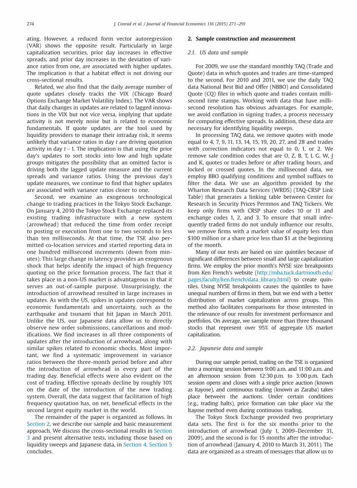
2.4.1. Variance ratioFollowing the notation in Lo and MacKinlay (1988),

define Xt as the log price process, where Xt¼X0, X1,…, XT.We refer to the price process in generic terms, although inimplementation we use NBBO quote midpoints to avoidnegative autocorrelation induced by bid-ask bounce. Forcross-sectional tests, we measure prices and returns over15-second and five-minute intervals, and we estimate theratio of the variance of these returns over measurementintervals of a half hour. There are 120 15-second returns ina half hour and we require at least 20 nonzero 15-secondreturns, to calculate a variance ratio. This ensures thatvariances, and therefore their ratios, are not degenerate.Our choice of measurement interval is determined by twotrade-offs. The interval needs to be short enough to mea-sure high-frequency changes in the supply curve, whilepreserving time of day effects. The interval also needs to belong enough to reliably measure contemporaneous var-iance ratios across a large sample of securities. A half-hourinterval is a reasonable balance between capturing high-frequency activity and this econometric necessity.2

Given the speed of the quote updating process, 15seconds could be too long an interval. In a robustnesscheck, we also measure variance ratios using one hundredmilliseconds and one- or two-second returns for stocks inthe largest size quintile. We do so only for large cap stocksbecause, in other securities, quote midpoints do notchange enough in successive one hundred millisecondintervals to provide a reliable measure of the variance ofreturns. In addition, for calculating variance ratios aroundliquidity sweeps, we use the variability of quote midpointsat one and 15-second intervals, in a three hundred secondperiod before and after each sweep.

Each return interval is equally spaced so that there areT¼nq returns in the measurement interval, where n and qare integers greater than one. The number of non-over-lapping long-horizon returns in the measurement intervalis n and q represents the number of non-overlappingshort-horizon intervals that are in the long-horizon return.There are T�qþ1 overlapping returns in the data. Com-paring midpoint sampling intervals, we generally haveq¼10 or 20 in our tests [see Lo and MacKinlay (1989) fora discussion of the choice of q]. Given this, the estimate ofthe mean drift in prices is

μ̂¼ 1nq

Xnqk ¼ 1

Xk�Xk�1ð Þ ¼ 1nq

ðXnq�X0Þ ð1Þ

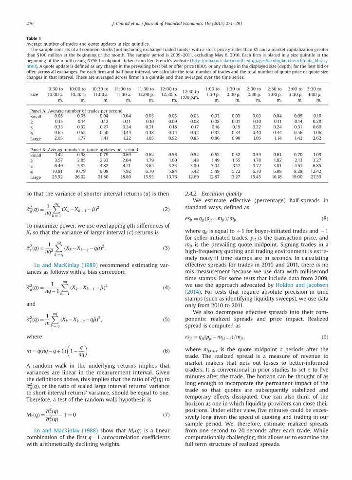
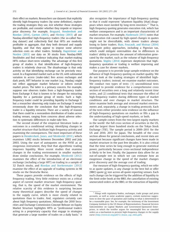
Table 1Average number of trades and quote updates in size quintiles.

The sample consists of all common stocks (not including exchange-traded funds), with a stock price greater than $1 and a market capitalization greaterthan $100 million at the beginning of the month. The sample period is 2009–2011, excluding May 6, 2010. Each firm is placed in a size quintile at thebeginning of the month using NYSE breakpoints taken from Ken French's website (http://mba.tuck.dartmouth.edu/pages/faculty/ken.french/data_library.html). A quote update is defined as any change in the prevailing best bid or offer price (BBO), or any change in the displayed size (depth) for the best bid oroffer, across all exchanges. For each firm and half hour interval, we calculate the total number of trades and the total number of quote price or quote sizechanges in that interval. These are averaged across firms in a quintile and then averaged over the time series.

Size9:30 to10:00 a.

m.

10:00 to10:30 a.

m.

10:30 to11:00 a.

m.

11:00 to11:30 a.

m.

11:30 to12:00 p.

m.

12:00 to12:30 p.

m.

12:30 to1:00 p.m.

1:00 to1:30 p.

m.

1:30 to2:00 p.

m.

2:00 to2:30 p.

m.

2:30 to3:00 p.

m.

3:00 to3:30 p.

m.

3:30 to4:00 p.

m.

Panel A: Average number of trades per secondSmall 0.05 0.05 0.04 0.04 0.03 0.03 0.03 0.03 0.03 0.03 0.04 0.05 0.102 0.15 0.14 0.12 0.11 0.10 0.09 0.08 0.08 0.01 0.10 0.11 0.14 0.283 0.33 0.32 0.27 0.24 0.21 0.18 0.17 0.18 0.19 0.22 0.24 0.31 0.604 0.65 0.62 0.50 0.44 0.38 0.34 0.32 0.32 0.34 0.40 0.44 0.56 1.06Large 2.05 1.77 1.41 1.22 1.05 0.92 0.85 0.86 0.90 1.05 1.14 1.42 2.62

Panel B: Average number of quote updates per secondSmall 1.42 0.98 0.79 0.69 0.62 0.56 0.52 0.52 0.52 0.59 0.61 0.70 1.092 3.57 2.85 2.33 2.04 1.79 1.60 1.48 1.49 1.55 1.78 1.82 2.13 3.273 6.49 5.82 4.82 4.21 3.64 3.23 3.00 3.04 3.17 3.72 3.81 4.51 6.854 10.81 10.79 9.08 7.92 6.70 5.84 5.42 5.49 5.72 6.70 6.99 8.28 12.42Large 25.52 26.02 21.80 18.80 15.93 13.76 12.69 12.87 13.27 15.45 16.18 19.00 27.55

J. Conrad et al. / Journal of Financial Economics 116 (2015) 271–291276

so that the variance of shorter interval returns (a) is then

σ̂2aðqÞ ¼

1nq

Xnqk ¼ 1

ðXk�Xk�1� μ̂Þ2 ð2Þ

To maximize power, we use overlapping qth differences ofXt so that the variance of larger interval (c) returns is

σ̂2c ðqÞ ¼

1nq2

Xnqk ¼ q

ðXk�Xk�q�qμ̂Þ2: ð3Þ

Lo and MacKinlay (1989) recommend estimating var-iances as follows with a bias correction:

σ2aðqÞ ¼

1nq�1

Xnqk ¼ 1

ðXk�Xk�1� μ̂Þ2 ð4Þ

and

σ2c ðqÞ ¼

1m

Xnqk ¼ q

ðXk�Xk�q�qμ̂Þ2; ð5Þ

where

m¼ q nq�qþ1ð Þ 1� qnq

� �ð6Þ

A random walk in the underlying returns implies thatvariances are linear in the measurement interval. Giventhe definitions above, this implies that the ratio of σ2

c ðqÞ toσ2aðqÞ, or the ratio of scaled large interval returns' variance

to short interval returns' variance, should be equal to one.Therefore, a test of the random walk hypothesis is

Mr qð Þ � σ2c ðqÞ

σ2aðqÞ

�1¼ 0 ð7Þ

Lo and MacKinlay (1988) show that MrðqÞ is a linearcombination of the first q�1 autocorrelation coefficientswith arithmetically declining weights.

2.4.2. Execution qualityWe estimate effective (percentage) half-spreads in

standard ways, defined as

esjt ¼ qjtðpjt�mjtÞ=mjt ð8Þ

where qjt is equal to þ1 for buyer-initiated trades and �1for seller-initiated trades, pjt is the transaction price, andmjt is the prevailing quote midpoint. Signing trades in ahigh-frequency quoting and trading environment is extre-mely noisy if time stamps are in seconds. In calculatingeffective spreads for trades in 2010 and 2011, there is nomis-measurement because we use data with millisecondtime stamps. For some tests that include data from 2009,we use the approach advocated by Holden and Jacobsen(2014). For tests that require absolute precision in timestamps (such as identifying liquidity sweeps), we use dataonly from 2010 to 2011.

We also decompose effective spreads into their com-ponents: realized spreads and price impact. Realizedspread is computed as

rsjt ¼ qjtðpjt�mj;tþ τÞ=mjt ; ð9Þ

where mj,tþτ is the quote midpoint τ periods after thetrade. The realized spread is a measure of revenue tomarket makers that nets out losses to better-informedtraders. It is conventional in prior studies to set τ to fiveminutes after the trade. The horizon can be thought of aslong enough to incorporate the permanent impact of thetrade so that quotes are subsequently stabilized andtemporary effects dissipated. One can also think of thehorizon as one in which liquidity providers can close theirpositions. Under either view, five minutes could be exces-sively long given the speed of quoting and trading in oursample period. We, therefore, estimate realized spreadsfrom one second to 20 seconds after each trade. Whilecomputationally challenging, this allows us to examine thefull term structure of realized spreads.

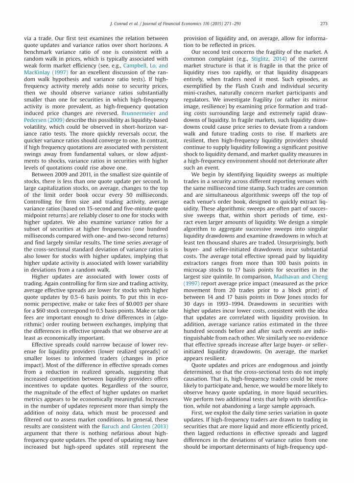
Table 2Average variance ratios for size quintiles.

The sample consists of all common stocks, with a stock price greater than $1 and a market capitalization greater than $100 million at the beginning of themonth from 2009 to 2011, excluding May 6, 2010. A quote update is defined as any change in the prevailing best bid or offer price (BBO), or any change inthe displayed size (depth) for the best bid or offer, across all exchanges. For each firm and half-hour interval, we use the median number of quote updatesto separate firms into low and high update groups (within each size quintile). For each firm and subsequent half-hour interval, we calculate variance ratiosbased on 15-second and five minute quote National Best Bid and Offer midpoints. The table shows time series averages of these group variance ratios. Thetime series average of the cross-sectional standard deviation is in parentheses.

QuintileUpdategroup

10:00 to10:30 a.

m.

10:30 to11:00 a.

m.

11:00 to11:30 a.

m.

11:30 to12:00 p.

m.

12:00 to12:30 p.

m.

12:30 to1:00 p.m.

1:00 to1:30 p.

m.

1:30 to2:00 p.

m.

2:00 to2:30 p.m.

2:30 to3:00 p.

m.

3:00 to3:30 p.m.

3:30 to4:00 p.

m.

Small Low 0.81 0.78 0.77 0.76 0.74 0.73 0.74 0.74 0.74 0.75 0.76 0.79(0.61) (0.60) (0.60) (0.59) (0.58) (0.57) (0.58) (0.57) (0.56) (0.57) (0.57) (0.57)

High 0.87 0.87 0.86 0.84 0.82 0.80 0.80 0.80 0.80 0.81 0.82 0.84(0.60) (0.60) (0.59) (0.59) (0.58) (0.57) (0.56) (0.56) (0.55) (0.55) (0.55) (0.56)

2 Low 0.99 0.98 0.97 0.97 0.94 0.94 0.94 0.94 0.91 0.94 0.93 0.91(0.63) (0.64) (0.63) (0.63) (0.61) (0.61) (0.60) (0.60) (0.58) (0.59) (0.58) (0.58)

High 0.99 1.00 0.98 0.99 0.95 0.94 0.94 0.93 0.90 0.92 0.90 0.88(0.60) (0.61) (0.61) (0.62) (0.60) (0.59) (0.58) (0.58) (0.54) (0.55) (0.54) (0.54)

3 Low 1.06 1.06 1.06 1.06 1.04 1.02 1.02 1.02 0.97 0.98 0.96 0.92(0.65) (0.66) (0.66) (0.66) (0.65) (0.64) (0.63) (0.63) (0.58) (0.59) (0.57) (0.56)

High 1.04 1.05 1.06 1.08 1.04 1.02 1.01 1.01 0.95 0.95 0.92 0.91(0.62) (0.63) (0.63) (0.65) (0.63) (0.61) (0.60) (0.60) (0.55) (0.55) (0.53) (0.53)

4 Low 1.09 1.10 1.10 1.11 1.08 1.06 1.05 1.04 1.00 0.99 0.97 0.95(0.66) (0.68) (0.68) (0.69) (0.67) (0.65) (0.65) (0.63) (0.59) (0.59) (0.57) (0.56)

High 1.05 1.05 1.08 1.10 1.07 1.05 1.04 1.03 0.97 0.98 0.95 0.96(0.62) (0.62) (0.64) (0.65) (0.64) (0.62) (0.60) (0.60) (0.55) (0.55) (0.53) (0.54)

Large Low 1.09 1.09 1.11 1.12 1.09 1.07 1.06 1.05 1.00 0.99 0.99 1.01(0.65) (0.65) (0.67) (0.68) (0.65) (0.64) (0.62) (0.62) (0.57) (0.57) (0.55) (0.56)

High 1.04 1.03 1.06 1.08 1.06 1.05 1.04 1.03 0.98 0.99 0.99 1.02(0.58) (0.59) (0.60) (0.62) (0.60) (0.59) (0.58) (0.57) (0.53) (0.53) (0.52) (0.53)

J. Conrad et al. / Journal of Financial Economics 116 (2015) 271–291 277

We also calculate the losses to better-informed traders,or price impact, as

pijt ¼ qjtðmj;tþ τ�mj;tÞ=mjt ð10ÞRealized spreads and price impact represent a decom-

position of effective spreads. The identity describing theirrelation is exact at particular points in this term structure(values of τ), such that esjt¼rsjtþpijt.

3. Cross-sectional results

3.1. Quotation and trading activity

We calculate the average number of trades and quoteupdates across securities in a size quintile in a half-hourinterval and then average over the entire time series. Panel Aof Table 1 shows the average number of trades per secondand Panel B shows the average number of quote updatesper second. Given our data filters in Section 2.1, each quintileis well diversified across a large number of firms. The smallestsize quintile has the largest number of firms due to the use ofNYSE size breaks and typically contains micro-cap stocks.Generally, quintiles 4 and 5 contain over 80% of the aggregatemarket capitalization. For readers interested in efficiencyoutside of small stocks, focusing on these quintiles is adequateto conduct inferences.

The average number of trades and quote updates increasesmonotonically from small to large firms. The magnitude of theincreases is notable. For instance, between 1:00 p.m. and 1:30,there are 0.03 trades per second (or 54 trades in the half hour)for the smallest market capitalization securities. In contrast,for stocks in the largest size quintile, there is almost one trade

per second. This velocity of trading increases sharply at thebeginning and end of the trading day. In the last half hour ofthe trading day when liquidity demands are particularly high,there are over two trades per second in the stocks in thelargest size quintile.

Panel B shows the number of quote updates. There aremonotonic increases in quote updates across size quintiles.Focusing again on the 1:00 p.m. to 1:30 window, there are0.52 quote updates per second in the smallest size quintileand more than 12 quote updates per second in the largestsize quintile. In general, the data show that changes to thetop of the book are an order of magnitude faster thantrades. Quoting occurs at a much higher frequency thantrading. The speed of these changes underscores theimportance of execution risk and latency.

3.2. Quote updates and variance ratios

We sort all stocks within a size quintile into low and highupdate groups in each half hour based on the median numberof updates in the prior half hour. We calculate the cross-sectional average variance ratio in each half hour and reportthe time series mean of these cross-sectional averages inTable 2. The standard errors of these means are extremelysmall because of the averaging of variance ratios over largenumbers of stocks. To provide a sense of variability, we reporttime series averages of the cross-sectional standard deviationsof variance ratios in parentheses.

Outside of microcap stocks (Size Quintile 1), averagevariance ratios are close to one. For all intents and purposes,an investor seeking to trade securities in these groups canexpect prices to behave, on average, as a random walk over

Fig. 1. Average variance ratios of stocks in low and high update groups within size and trade quintiles. Stocks are sorted into size quintile based on priormonth NYSE breakpoints and within size groups into quintiles based on the number of trades in each half hour. For example, Size1Trade1 contains firms inthe smallest size and trade quintile. Within these 25 (5�5) groups, stocks are further sorted into low and high update groups, using the median number ofupdates. We calculate average variance ratios for all stocks within a group and plot the time series average of these cross-sectional means.

J. Conrad et al. / Journal of Financial Economics 116 (2015) 271–291278

the horizons that we examine. We also calculate (but do notreport) first order autocorrelations of 15 second quotemidpoint returns. These autocorrelations are largely indis-tinguishable from zero. We also calculate but do not reportvariance ratios and autocorrelations based on transactionprices. As expected, they are influenced by bid-ask bounce.

Our interest is in the difference in variance ratiosbetween high and low update groups. In the vast majorityof cases, variance ratios in the high update groups arecloser to one than in the low update group. For example, inthe two largest size quintiles, which contain the majorityof the market capitalization of the US equity markets,average variance ratios are closer to one in high updategroups for 17 out of 24 half-hour estimates. In two cases,the average variance ratios are identical, and in five cases,high update groups have variance ratios that are furtherfrom one. Average cross-sectional standard deviations arealso systematically lower for high update groups. In thetwo largest size quintiles, the cross-sectional standarddeviation is lower for high update groups in all 24 cases.

3.3. Separating quote updates from trades

Quote updates can come from additions and cancella-tions of orders to the order book or from trades thatextract liquidity. One could argue that controlling fortrading is unnecessary because all changes to the supplycurve are legitimate, regardless of whether they are due to

submissions or cancellations or trading. Nonetheless, it isimportant to understand whether it is differences in thetrading frequency across these groups that drive therelation we observe. Within each size quintile, we sort allstocks in a half hour interval into quintiles based on thenumber of trades in that interval. Then, within each tradequintile, we further separate stocks into low and highupdate groups based on the median number of quoteupdates in the prior half hour. This dependent sortprocedure results in 50 groups (5�5�2) and allows usto see the effect of increased quotation activity, holdingsize and trading activity roughly constant.

Displaying such a large number of estimates is anexpositional challenge so we employ two approaches todescribe our results. Fig. 1 shows average variance ratiosfor each size and trade quintile, with separate bars for lowand high update groups. The graph shows that, across allsize and trade quintiles, average variance ratios are gen-erally closer to one for high update groups. Fig. 2 shows asimilarly constructed bar graph for the average cross-sectional standard deviation of variance ratios. Cross-sectional standard deviations are systematically lower forhigh update groups in every size and trade quintile.

Table 3 contains formal statistics for these differences.Because our interest is in departures of variance ratiosfrom one, we calculate the absolute value of the differencein each stock's variance ratio from one (|VRi�1|) and thencompute cross-sectional averages for low and high update

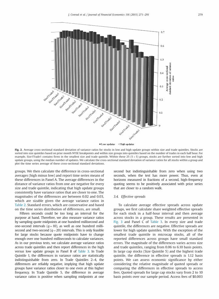
Fig. 2. Average cross-sectional standard deviation of variance ratios for stocks in low and high update groups within size and trade quintiles. Stocks aresorted into size quintiles based on prior month NYSE breakpoints and within size groups into quintiles based on the number of trades in each half hour. Forexample, Size1Trade1 contains firms in the smallest size and trade quintile. Within these 25 (5�5) groups, stocks are further sorted into low and highupdate groups, using the median number of updates. We calculate the cross-sectional standard deviation of variance ratios for all stocks within a group andplot the time series average of these cross-sectional standard deviations.

J. Conrad et al. / Journal of Financial Economics 116 (2015) 271–291 279

groups. We then calculate the difference in cross-sectionalaverages (high minus low) and report time series means ofthese differences in Panel A. The average differences in thedistance of variance ratios from one are negative for everysize and trade quintile, indicating that high update groupsconsistently have variance ratios that are closer to one. Themagnitudes of the differences are between 0.02 and 0.03,which are sizable given the average variance ratios inTable 2. Standard errors, which are conservative and basedon the time series distribution of differences, are small.

Fifteen seconds could be too long an interval for thepurpose at hand. Therefore, we also measure variance ratiosby sampling quote midpoints at one hundred millisecond andone-second intervals (q¼10), as well as one hundred milli-second and two-second (q¼20) intervals. This is only feasiblefor large stocks because quote midpoints have to changeenough over one hundred milliseconds to calculate variances.As in our previous tests, we calculate average variance ratiosacross trade quintiles and then report differences in the highversus low update groups in Panel B of Table 3. In TradeQuintile 1, the differences in variance ratios are statisticallyindistinguishable from zero. In Trade Quintiles 2–4, thedifferences are reliably negative, implying that high updategroups have variance ratios closer to one even at this higherfrequency. In Trade Quintile 5, the difference in averagevariance ratios is positive when sampling midpoints at one

second but indistinguishable from zero when using twoseconds, when the test has more power. Thus, even athorizons measured in fractions of a second, high-frequencyquoting seems to be positively associated with price seriesthat are closer to a random walk.

3.4. Effective spreads

To calculate average effective spreads across updategroups, we first calculate share weighted effective spreadsfor each stock in a half-hour interval and then averageacross stocks in a group. These results are presented inFig. 3 and Panel C of Table 3. In every size and tradequintile, the differences are negative. Effective spreads arelower for high update quintiles. With the exception of thesmallest trade quintile in microcap stocks, all of thereported differences across groups have small standarderrors. The magnitude of the differences varies across sizeand trade quintiles, ranging from 0.06 to 6.10 basis points.In large cap stocks (Size Quintile 5) and the highest tradequintile, the difference in effective spreads is 1.12 basispoints. We can assess economic significance by eitherconsidering the relative magnitude of quoted spreads orcomparing the differences in effective spreads to accessfees. Quoted spreads for large cap stocks vary from 2 to 10basis points over our sample period. Access fees of $0.003

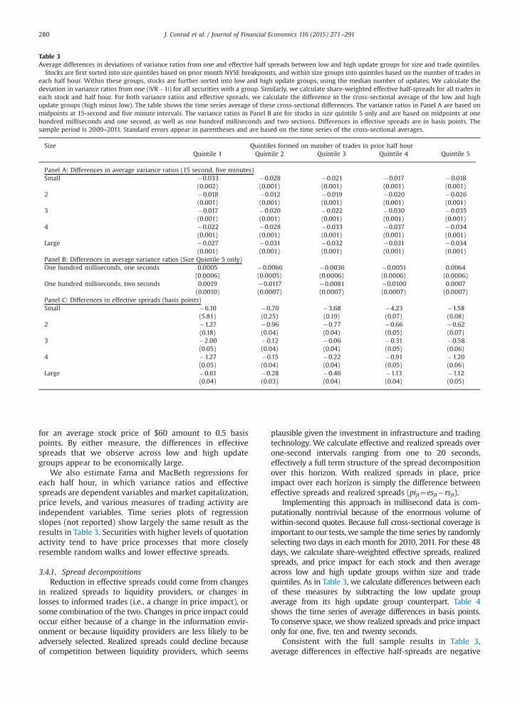
Table 3Average differences in deviations of variance ratios from one and effective half spreads between low and high update groups for size and trade quintiles.

Stocks are first sorted into size quintiles based on prior month NYSE breakpoints, and within size groups into quintiles based on the number of trades ineach half hour. Within these groups, stocks are further sorted into low and high update groups, using the median number of updates. We calculate thedeviation in variance ratios from one (|VR�1|) for all securities with a group. Similarly, we calculate share-weighted effective half-spreads for all trades ineach stock and half hour. For both variance ratios and effective spreads, we calculate the difference in the cross-sectional average of the low and highupdate groups (high minus low). The table shows the time series average of these cross-sectional differences. The variance ratios in Panel A are based onmidpoints at 15-second and five minute intervals. The variance ratios in Panel B are for stocks in size quintile 5 only and are based on midpoints at onehundred milliseconds and one second, as well as one hundred milliseconds and two sections. Differences in effective spreads are in basis points. Thesample period is 2009–2011. Standard errors appear in parentheses and are based on the time series of the cross-sectional averages.

Size Quintiles formed on number of trades in prior half hourQuintile 1 Quintile 2 Quintile 3 Quintile 4 Quintile 5

Panel A: Differences in average variance ratios (15 second, five minutes)Small �0.033 �0.028 �0.021 �0.017 �0.018

(0.002) (0.001) (0.001) (0.001) (0.001)2 �0.018 �0.012 �0.019 �0.020 �0.026

(0.001) (0.001) (0.001) (0.001) (0.001)3 �0.017 �0.020 �0.022 �0.030 �0.035

(0.001) (0.001) (0.001) (0.001) (0.001)4 �0.022 �0.028 �0.033 �0.037 �0.034

(0.001) (0.001) (0.001) (0.001) (0.001)Large �0.027 �0.031 �0.032 �0.031 �0.034

(0.001) (0.001) (0.001) (0.001) (0.001)Panel B: Differences in average variance ratios (Size Quintile 5 only)One hundred milliseconds, one seconds 0.0005 �0.0066 �0.0036 �0.0051 0.0064

(0.0006) (0.0005) (0.0006) (0.0006) (0.0006)One hundred milliseconds, two seconds 0.0019 �0.0117 �0.0081 �0.0100 0.0007

(0.0010) (0.0007) (0.0007) (0.0007) (0.0007)Panel C: Differences in effective spreads (basis points)Small �6.10 �0.70 �3.68 �4.23 �1.58

(5.81) (0.25) (0.19) (0.07) (0.08)2 �1.27 �0.96 �0.77 �0.66 �0.62

(0.18) (0.04) (0.04) (0.05) (0.07)3 �2.00 �0.12 �0.06 �0.31 �0.58

(0.05) (0.04) (0.04) (0.05) (0.06)4 �1.27 �0.15 �0.22 �0.91 �1.20

(0.05) (0.04) (0.04) (0.05) (0.06)Large �0.61 �0.28 �0.46 �1.13 �1.12

(0.04) (0.03) (0.04) (0.04) (0.05)

J. Conrad et al. / Journal of Financial Economics 116 (2015) 271–291280

for an average stock price of $60 amount to 0.5 basispoints. By either measure, the differences in effectivespreads that we observe across low and high updategroups appear to be economically large.

We also estimate Fama and MacBeth regressions foreach half hour, in which variance ratios and effectivespreads are dependent variables and market capitalization,price levels, and various measures of trading activity areindependent variables. Time series plots of regressionslopes (not reported) show largely the same result as theresults in Table 3. Securities with higher levels of quotationactivity tend to have price processes that more closelyresemble random walks and lower effective spreads.

3.4.1. Spread decompositionsReduction in effective spreads could come from changes

in realized spreads to liquidity providers, or changes inlosses to informed trades (i.e., a change in price impact), orsome combination of the two. Changes in price impact couldoccur either because of a change in the information envir-onment or because liquidity providers are less likely to beadversely selected. Realized spreads could decline becauseof competition between liquidity providers, which seems

plausible given the investment in infrastructure and tradingtechnology. We calculate effective and realized spreads overone-second intervals ranging from one to 20 seconds,effectively a full term structure of the spread decompositionover this horizon. With realized spreads in place, priceimpact over each horizon is simply the difference betweeneffective spreads and realized spreads (pijt¼esjt�rsjt).

Implementing this approach in millisecond data is com-putationally nontrivial because of the enormous volume ofwithin-second quotes. Because full cross-sectional coverage isimportant to our tests, we sample the time series by randomlyselecting two days in each month for 2010, 2011. For these 48days, we calculate share-weighted effective spreads, realizedspreads, and price impact for each stock and then averageacross low and high update groups within size and tradequintiles. As in Table 3, we calculate differences between eachof these measures by subtracting the low update groupaverage from its high update group counterpart. Table 4shows the time series of average differences in basis points.To conserve space, we show realized spreads and price impactonly for one, five, ten and twenty seconds.

Consistent with the full sample results in Table 3,average differences in effective half-spreads are negative

Fig. 3. Average effective spreads in basis points for stocks in low and high update groups within size and trade quintiles. Stocks are sorted into size quintilebased on prior month NYSE breakpoints and within size groups into quintiles based on the number of trades in each half hour. For example, Size1Trade1contains firms in the smallest size and trade quintile. Within these 25 (5�5) groups, stocks are further sorted into low and high update groups, using themedian number of updates. We calculate share-weighted effective half-spreads for all stocks within a group and plot the time series average of these cross-sectional means.

J. Conrad et al. / Journal of Financial Economics 116 (2015) 271–291 281

for most size and trade quintiles.3 In Size Quintiles 1–3,most of the reduction in effective spreads comes fromdecreases in realized spreads. In Size Quintiles 4 and 5, thereductions in effective spreads themselves are smaller, butthey are still due to declines in realized spreads. Theseresults are in contrast to those reported by Hendershott,Jones, and Menkveld (2011), who report increases inrealized spreads between 2001 and 2005, suggesting thatliquidity providers (at least temporarily) earned greaterrevenues after the advent of autoquoting. The decline inrealized spreads that we find also differs from the resultsin Riordan and Storkenmaier (2011), who find a sharp andpersistent increase in realized spreads following a systemupgrade on Deutsche Borse that resulted in a decline inlatency. Our results suggest that, between 2009 and 2011,

3 The effective spreads calculated from millisecond data are lessvariable than the effective spreads in Table 3, which includes both thesecond data (2009) and the millisecond data (2010, 2011). We conjecturethat the higher variability is a result of noise in signing trades when non-millisecond data are used. To test this, we repeat our tests in Table 3 usingonly 2010, 2011 millisecond data and find that standard errors are muchsmaller. The general pattern of differences in effective spreads betweenhigh and low update groups remains similar.

competition between electronic liquidity providers app-ears to be sufficient to generate reductions in realizedspreads for those securities with a higher-speed tradingenvironment.

3.5. Liquidity drawdowns and market resiliency

In resilient markets, large drawdowns of liquidity shouldminimally influence the future supply of liquidity. One couldlook ex post at cases in which there are dramatic changes inprices seemingly caused by innocuously small trades. This isthe approach that some market participants take to highlightaspects of market structure to either regulators or the press. Agood example is individual flash crashes systematicallyshown by Nanex on its website (http://www.nanex.net/FlashCrashEquities/FlashCrashAnalysis_Equities.html). Themethod we describe below provides results that are morerepresentative of the conditions faced by market participantsin a large cross section of securities. Our approach does notrequire cherry-picking the data on price changes or measuresof market quality, allowing for general inferences.

We employ a three-step procedure to isolate large liquid-ity drawdowns that exploits the millisecond resolution of thedata. We first identify multiple trades in a stock with the

Table 4Average differences in effective half-spreads, realized spreads and price impact between low and high update groups for size and trade quintiles.

Effective spreads are calculated as the scaled difference between the transaction price and prevailing quote midpoint. Realized spreads are computed asthe price movement from transaction prices to a future quote midpoint, scaled by the midpoint prevailing at the time of the transaction. We use quotemidpoints one, five, ten, and 20 seconds after the trade. Price impact is the difference between the effective spread of the transaction and its realizedspread. For each stock, we calculate share-weighted average effective spreads, realized spreads, and price impact. We compute cross-sectional averages forstocks in each size quintile, trade quintile, and update group. We then calculate the differences between these cross-sectional averages between low andhigh update groups (high minus low). The table shows the time series averages of these differences for each size and trade quintile. All estimates are inbasis points. The sample consists of all stocks in these groups for two randomly selected trading days in each month for 2010–2011.

Size quintile Trade quintile Effective spreads Realized spreads Price impact

Tþ1 Tþ5 Tþ10 Tþ20 Tþ1 Tþ5 Tþ10 Tþ20

Small 1 �36.7 �14.0 �14.6 �14.2 �13.8 �22.7 �22.1 �22.5 �22.92 �11.5 �4.9 �5.5 �5.4 �5.3 �6.6 �6.0 �6.1 �6.23 �7.2 �5.3 �5.4 �5.2 �5.0 �1.9 �1.8 �2.0 �2.24 �7.5 �5.5 �5.3 �5.1 �4.8 �2.0 �2.2 �2.4 �2.75 �4.7 �3.7 �3.7 �3.6 �3.4 �1.0 �1.0 �1.1 �1.3

2 1 �4.3 �2.4 �2.7 �2.6 �2.5 �1.9 �1.6 �1.7 �1.82 �1.0 �0.9 �0.9 �0.9 �0.9 �0.1 �0.1 �0.1 �0.13 �1.1 �0.8 �0.8 �0.8 �0.8 �0.3 �0.3 �0.3 �0.34 �1.0 �0.9 �0.9 �0.9 �0.8 �0.1 �0.1 �0.1 �0.25 �0.7 �0.5 �0.8 �0.7 �0.7 �0.2 0.1 0.0 0.0

3 1 �2.7 �1.6 �1.6 �1.6 �1.5 �1.1 �1.1 �1.1 �1.22 �0.4 �0.5 �0.5 �0.5 �0.5 0.1 0.1 0.1 0.13 �0.4 �0.4 �0.4 �0.4 �0.4 0.0 0.0 0.0 0.04 �0.3 �0.3 �0.4 �0.4 �0.4 0.0 0.1 0.1 0.15 �0.4 �0.4 �0.6 �0.5 �0.5 0.0 0.2 0.1 0.1

4 1 �0.7 �0.6 �0.5 �0.5 �0.4 �0.1 �0.2 �0.2 �0.32 �0.1 0.0 �0.1 �0.1 �0.1 �0.1 0.0 0.0 0.03 0.0 0.0 �0.1 �0.1 �0.1 0.0 0.1 0.1 0.14 �0.1 �0.1 �0.2 �0.2 �0.2 0.0 0.1 0.1 0.15 �0.3 �0.3 �0.5 �0.4 �0.4 0.0 0.2 0.1 0.1

Large 1 �0.1 �0.1 �0.1 �0.1 �0.1 0.0 0.0 0.0 0.02 0.1 0.1 �0.1 �0.1 �0.1 0.0 0.2 0.2 0.23 �0.1 0.0 �0.1 �0.1 �0.1 �0.1 0.0 0.0 0.04 �0.2 �0.2 �0.2 �0.2 �0.1 0.0 0.0 0.0 �0.15 �0.2 �0.1 �0.1 0.0 0.0 �0.1 �0.1 �0.2 �0.2

J. Conrad et al. / Journal of Financial Economics 116 (2015) 271–291282

same millisecond timestamp across more than one reportingvenue (“sweeps”). We then aggregate individual sweeps thatoccur within short durations of each other into “collapsed”sweeps, and focus exclusively on those that extract largeamounts of liquidity. Details of the process aredescribed below.

In the first step, we isolate multiple trades with thesame millisecond time stamp that originates from differ-ent reporting venues. It is critical that trades take place indifferent venues to ensure that multiple trades with thesame millisecond time stamp are not a mechanical artifactof trade reporting and splitting procedures, as would begenerated by one large order interacting with multiplesmall counterparty orders on a single limit order book.Trades across multiple venues in the same millisecond arealgorithmic in nature, sweeping the top of various orderbooks in dark or lit markets, and represent attempts torapidly extract liquidity. During our sample period, thereare 764 million such liquidity sweeps, accounting for $17.6trillion in volume.

In small stocks, sweeps represent 13% of total volume,rising almost monotonically to 22% for large stocks. Givenfragmentation and the speed at which quotes change,trading algorithms that attempt to extract liquidity quickly

across multiple venues must exercise particular care to notviolate the trade-through rule of Reg NMS. We observeconsiderable use of intermarket sweep orders (ISOs) inalgorithmic sweeps, and although not reported, the datashow an increase in the size of sweeps and the use of ISOsover time.

We separate the sample of sweeps into buyer- andseller-initiated sweeps, so that the trading we analyzerepresents rapid drawdowns on either the bid or ask sideof the limit order book (and not just fast random trades onboth sides of the market). The median time differencebetween successive sweeps in small cap stocks is 22seconds, falling monotonically across size quintiles to only0.8 seconds in large cap stocks. Sweeps on one side of themarket, which occur so closely to one another, are unlikelyto be independent. Typical trading algorithms generatewaves of child orders that are conditioned on priorexecutions and desired volume (among other parameters).Therefore, the second step of the procedure we use aggr-egates closely timed sequential sweeps. To do so, we firstcalculate the expected time between trades as the mediantime between trades for each stock-half-hour in the priormonth. We then cumulate consecutive buy or sell sweepstogether if the time between adjacent sweeps is less than

Fig. 4. Collapsing consecutive sweeps. In this illustration, the time line is in seconds, and the median time between trades in the prior month and the samehalf-hour interval is one second. S refers to a sweep and T stands for a trade. Consecutive sweeps that take place with an inter-sweep time of one secondare collapsed together.

J. Conrad et al. / Journal of Financial Economics 116 (2015) 271–291 283

its expected value. A graphical illustration of this process isprovided in Fig. 4.

By construction, aggregated sweeps are larger andinter-sweep time differences are greater. To focus on largeliquidity demands, we further restrict the sample toaggregated sweeps that cumulatively extract ten thousandshares. There are two reasons to impose this restriction.First, it corresponds to the cutoff for block trades in theupstairs market in the era of preelectronic trading. Second,it allows for comparisons with the extensive literature onthe liquidity and price discovery effects of such blocktrades. The final sample consists of about 4.4 millionaggregated sweeps. The average time between successiveaggregated sweeps ranges from 2,456 seconds for SizeQuintile 1 to 454 seconds for Size Quintile 5.4

Our interest is in the extent to which the market is ableto absorb such liquidity shocks without experiencingsignificant changes in the price formation process. To thatend, we estimate variance ratios before and after theselarge liquidity sweeps. This poses implementation chal-lenges. We need an appropriate time horizon over whichto measure returns. To preserve independence, the pre-and post-measurement interval needs to be short enoughso that there is minimal overlap in successive sweeps inthe same stock. Given this consideration, and the distribu-tion of the time differences between consecutive sweeps,we define pre- and post-sweep periods as three hundredseconds. Pre-sweep periods include all observations up tothe beginning of the sweep, and post-sweep observationscommence immediately after the end of the sweep. Formeasuring variance ratios, this allows us to sample quotemidpoints at one second and 15-second intervals (q¼15).We impose the additional constraint that there be at least15 nonzero returns in each three hundred second intervalto calculate variance ratios.

Panel A of Table 5 shows average values of |VRt�1| beforeand after large liquidity sweeps. Average pre- and post-sweepestimates of variance ratios are substantially different fromone, and from the unconditional averages in Table 2. Therelatively high variance over short horizons implied by thesevariance ratios is consistent with the liquidity-based volatility

4 We also identify large sweeps using a stock specific approach. Wecompute a relative volume ratio as the number of shares traded in thecollapsed sweep, scaled by the product of average trade size (in shares) inthe prior month multiplied and the number of trades. We then considerlarge sweeps as those above the 95th percentile in the distribution of thisrelative volume ratio. Such a definition includes many liquidity sweepsthat are smaller than ten thousand shares.

that Brunnermeier and Pedersen (2009) describe. However, itis also related to a more subtle aspect of our short-horizonvariance ratio measure. Recall that variances can be com-puted only if quote midpoints move enough (i.e., that thevariance measure in returns is non-degenerate) and that werequire at least 15 nonzero returns to calculate varianceratios. In our sample, quote midpoints exhibit very littlemovement at the one and 15-second horizon in the threehundred second interval before or after an aggregated sweep.For example, even in large cap stocks, we are able to reliablycalculate variance ratios for only 31% of the sample. That is,the short-horizon variance measures used in our calculationof variance ratios around sweeps are biased toward largerprice movements, and the relative magnitude of the biasincreases for shorter horizons. This implies that our varianceratio measures are biased downward.

With that in mind, our interest is primarily in changes invariance ratios around the liquidity drawdown. Panel A showsthat the values of Δ|VRt�1| are very close to zero. Unsurpris-ingly given the large sample sizes, paired t-statistics reject thenull that Δ|VRt�1| is different from zero. However, thedirection of the change in point estimates consistently showthat variance ratios improve slightly (instead of worsen) afterlarge drawdowns in liquidity.

Panel B shows share-weighted average effective spreads inthe three hudnred seconds before and after these largesweeps. We also report the total effective spread paid by alltrades within the sweep itself. Effective spreads before sweepsdecline with firm size from roughly 20 basis points to 3 basispoints. The average total effective spread, paid by thoseexecuting the sweep orders, ranges from around 120 basispoints (in Size Quintile 1) to 17 basis points (for Quintile 5).The latter is roughly similar in magnitude to the total price ofblock trades in Dow Jones stocks reported by Madhavan andCheng (1997). Post-sweep effective spreads are similar to thoseprior to the liquidity drawdown. Again, paired t-statistics rejectthe null of equality and, in all cases, the direction of thedifference is one in which effective spreads are lower after theliquidity event. It appears that investors are able to extractlarge amounts of liquidity from the market, with marketsreplenishing that liquidity quickly and the price discoveryprocess experiencing no significant ill effects.5

5 One could be concerned that requiring data before and after asweep could introduce a selection bias if sweeps cause a significantdecline in liquidity. In that situation, market data would be availablebefore a sweep but not after. We verify that this does not occur in oursample.

Table 5Average variance ratios and effective half spreads before and after large liquidity drawdowns.

The sample consists of all collapsed buyer- and seller-initiated liquidity sweeps in which more than ten thousand shares are traded. We calculatevariance ratios and share-weighted effective spreads three hundred seconds before the beginning of the aggregated sweep and three hundred secondsafter the end of the sweep. We also calculate the sum of effective spreads for all trades within the sweep. Panel A reports the absolute value of the distanceof the variance ratios from one, as well as the difference between the post- and pre-sweep variance ratios. Panel B reports simple averages of share-weighted pre- and post-sweep effective spreads, the intra-sweep effective spread, and the difference between the post- and pre-sweep effective spreads.All effective spreads are in basis points.

Panel A: |VR�1| before and after liquidity sweeps greater than 10,000 sharesPre-sweep Post-sweep Δ|VR�1| t-Statistic

Buyer-initiatedSmall 0.3133 0.3038 �0.0095 �2.882 0.3046 0.2948 �0.0097 �5.333 0.2991 0.2919 �0.0072 �5.114 0.3013 0.2946 �0.0066 �6.37Large 0.2696 0.2648 �0.0047 �14.90

Seller-initiatedSmall 0.3114 0.3085 �0.0028 �0.852 0.3034 0.2930 �0.0103 �5.863 0.2953 0.2899 �0.0054 �3.844 0.2950 0.2919 �0.0030 �2.99Large 0.2681 0.2642 �0.0039 �12.38Panel B: Average effective half-spreads around liquidity sweeps greater than ten thousand shares

Pre-sweep Intra-sweep Post-sweep Δ Effective spread t-Statistic

Buyer-initiatedSmall 20.10 121.59 17.80 �2.29 �3.412 10.16 65.30 9.30 �0.80 �8.053 7.61 49.73 6.93 �0.68 �8.214 6.08 34.26 5.24 �0.83 �7.38Large 3.04 17.18 2.68 �0.36 �9.68Seller-initiatedSmall 19.59 115.22 17.77 �1.85 �3.482 10.35 65.73 9.41 �0.93 �7.743 7.77 48.08 6.98 �0.71 �5.844 6.29 33.61 5.27 �1.02 �5.13Large 3.08 17.37 2.70 �0.38 �14.18

J. Conrad et al. / Journal of Financial Economics 116 (2015) 271–291284

Changes in the price process or trading costs before andafter sweeps could be fundamentally different for stockswith low versus high quote updates. Therefore, we alsocalculate changes in variance ratios and effective spreadsbefore, during, and after sweeps after placing each sweepinto the triple sorted size-trade update groupings used inTable 3. The changes in variance ratios and effective spreadsare small and negative, similar to those in Table 5 (andtherefore not reported in a separate table). There is, however,one key difference. Intrasweep effective spreads (i.e., the costof the liquidity drawdown) are significantly higher in groupswith fewer updates in the prior half hour, with differencesranging in value from 7 to 37 basis points. The implication,consistent with the cross-sectional results in Table 3, is thatupdate activity is associated with lower trading costs.

4. Alternative tests

The cross-sectional tests suggest that increased quota-tion activity is associated with variance ratios closer to oneand with lower costs of trading. Price efficiency, quotationactivity, and trading are all endogenous. Although wemeasure quotation activity prior to measuring varianceratios, this endogeneity could affect inferences. In this

section, we report results from tests that allow for causalinterpretations.

4.1. Exploiting time series variation in updates

Nagel (2012) reports that returns to supplying liquid-ity are strongly related to measures of fundamentalvolatility, such as VIX. If quote updates are the tool thatmarket makers use to manage their intraday risk expo-sure (as well as the returns that they earn), then updatesshould also be related to the VIX. We sum the number ofupdates for each firm-day and then average across firmsin a size quintile. Fig. 5 plots the daily time series, alongwith the VIX over the sample period. The graph showsthat the time series variation in updates is large and thatthe correlation of updates with the VIX is clear. Forexample, the high volatility period in August 2011 isaccompanied by large increases in updates. The localpeak in the average number of updates across all firmsand VIX on August 8 coincides with a 6.7% drop in theStandard and Poor's 500. This suggests that aggregateuncertainty has a role to play in the intensity of changesin the liquidity supply curve.

Fig. 5. Average number of quote updates per day for size quintiles. For each day, we sum the number of updates for each firm and then average across firmsin size quintiles. Daily closing values of the VIX (Chicago Board Options Exchange Market Volatility Index) are plotted using the right vertical axis.

J. Conrad et al. / Journal of Financial Economics 116 (2015) 271–291 285

We investigate these relations more formally using asimple reduced form vector autoregression of the form

ΔUpdt ¼X4i ¼ 1

βiΔUpdt� iþX4i ¼ 1

γiΔVIXt� iþX4i ¼ 1

κΔMQt� iþε1;t ;

ð11Þ

ΔVIXt ¼X4i ¼ 1

β0iΔUpdt� iþ

X4i ¼ 1

γ0iΔVIXt� iþX4i ¼ 1

κ0ΔMQt� iþε2;t ;

ð12Þand

ΔMQt ¼X4i ¼ 1

β0iΔUpdt� iþ

X4i ¼ 1

γ0iΔVIXt� iþX4i ¼ 1

κ0ΔMQt� iþε3;t

ð13Þwhere all changes are in percentages and MQ refers to ameasure of market quality. The system is estimated on dailydata from 2009 to 2011 separately for each size quintile.Simple specification checks (not reported) show that four lagsare adequate to capture the dependence structure.

Table 6 reports coefficients with Z-statistics in parenth-eses. In Panel A, market quality (MQ) is measured using thedeviations in variance ratios from one (Δ|VR�1|), and inPanel B, market quality is measured using effectivespreads. We draw two inferences from these regressions.First, we examine the time series relation between mea-sures of market quality and changes in updates. Considerthe possibility that, instead of increases in updates drivingincreases in liquidity and improvements in price discovery,the causation is reversed. High-frequency traders increasetheir activity in securities because those securities are

relatively more liquid and their prices are relatively moreefficient. Such a relation could occur because it is easier forHFTs to manage risk in such an environment. In that case,one would expect changes in updates in period t tobe negatively related to lagged changes in measures ofmarket quality. In Quintiles 1–4, most of the coefficientson lagged values of ΔMQ are statistically indistinguishablefrom zero in both panels. In Quintile 5, the coefficients onΔMQ are positive and, particularly for variance ratiosmeasures, statistically significant. That is, if lagged effec-tive spreads are higher, and lagged variance ratios arefurther from one, high frequency activity increases. Thisresult is more consistent with high-frequency tradersstepping in to provide liquidity and facilitate price dis-covery, instead of being attracted to improvements inliquidity and efficient pricing.

The second inference that we draw from these results isthat changes in updates are positively related to laggedinnovations in VIX. The econometric interpretation is thatchanges in VIX Granger-cause changes in updates. Theeconomic interpretation is that liquidity suppliers react tochanges in the risk environment by changing the fre-quency of updates. Beyond a one-day lag, the influenceof VIX wanes quickly. Interestingly, the VIX equationshows that changes in quote update activity do notGranger-cause changes in the VIX at any lag. This isinconsistent with the belief that high-frequency quotingor trading either generates or exacerbates measures ofmarket volatility.

The results of the VAR suggest another test that couldhelp control for endogeneity. Despite the fact that wemeasure variance ratios after calculating quote updates,

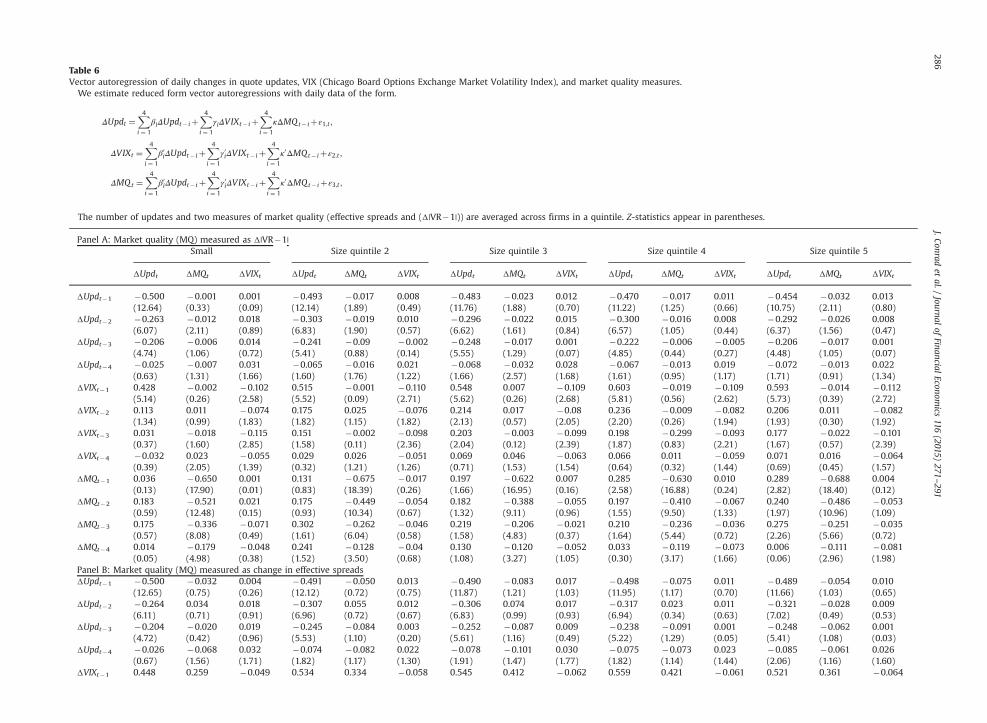
Table 6Vector autoregression of daily changes in quote updates, VIX (Chicago Board Options Exchange Market Volatility Index), and market quality measures.

We estimate reduced form vector autoregressions with daily data of the form.

ΔUpdt ¼X4i ¼ 1

βiΔUpdt� iþX4i ¼ 1

γiΔVIXt� iþX4i ¼ 1

κΔMQt� iþε1;t ;

ΔVIXt ¼X4i ¼ 1

β0iΔUpdt� iþX4i ¼ 1

γ0iΔVIXt� iþX4i ¼ 1

κ0ΔMQt� iþε2;t ;

ΔMQt ¼X4i ¼ 1

β0iΔUpdt� iþX4i ¼ 1

γ0iΔVIXt� iþX4i ¼ 1

κ0ΔMQt� iþε3;t ;

The number of updates and two measures of market quality (effective spreads and (Δ|VR�1|)) are averaged across firms in a quintile. Z-statistics appear in parentheses.

Panel A: Market quality (MQ) measured as Δ|VR�1|Small Size quintile 2 Size quintile 3 Size quintile 4 Size quintile 5

ΔUpdt ΔMQt ΔVIXt ΔUpdt ΔMQt ΔVIXt ΔUpdt ΔMQt ΔVIXt ΔUpdt ΔMQt ΔVIXt ΔUpdt ΔMQt ΔVIXt

ΔUpdt�1 �0.500 �0.001 0.001 �0.493 �0.017 0.008 �0.483 �0.023 0.012 �0.470 �0.017 0.011 �0.454 �0.032 0.013(12.64) (0.33) (0.09) (12.14) (1.89) (0.49) (11.76) (1.88) (0.70) (11.22) (1.25) (0.66) (10.75) (2.11) (0.80)

ΔUpdt�2 �0.263 �0.012 0.018 �0.303 �0.019 0.010 �0.296 �0.022 0.015 �0.300 �0.016 0.008 �0.292 �0.026 0.008(6.07) (2.11) (0.89) (6.83) (1.90) (0.57) (6.62) (1.61) (0.84) (6.57) (1.05) (0.44) (6.37) (1.56) (0.47)

ΔUpdt�3 �0.206 �0.006 0.014 �0.241 �0.09 �0.002 �0.248 �0.017 0.001 �0.222 �0.006 �0.005 �0.206 �0.017 0.001(4.74) (1.06) (0.72) (5.41) (0.88) (0.14) (5.55) (1.29) (0.07) (4.85) (0.44) (0.27) (4.48) (1.05) (0.07)

ΔUpdt�4 �0.025 �0.007 0.031 �0.065 �0.016 0.021 �0.068 �0.032 0.028 �0.067 �0.013 0.019 �0.072 �0.013 0.022(0.63) (1.31) (1.66) (1.60) (1.76) (1.22) (1.66) (2.57) (1.68) (1.61) (0.95) (1.17) (1.71) (0.91) (1.34)

ΔVIXt�1 0.428 �0.002 �0.102 0.515 �0.001 �0.110 0.548 0.007 �0.109 0.603 �0.019 �0.109 0.593 �0.014 �0.112(5.14) (0.26) (2.58) (5.52) (0.09) (2.71) (5.62) (0.26) (2.68) (5.81) (0.56) (2.62) (5.73) (0.39) (2.72)

ΔVIXt�2 0.113 0.011 �0.074 0.175 0.025 �0.076 0.214 0.017 �0.08 0.236 �0.009 �0.082 0.206 0.011 �0.082(1.34) (0.99) (1.83) (1.82) (1.15) (1.82) (2.13) (0.57) (2.05) (2.20) (0.26) (1.94) (1.93) (0.30) (1.92)

ΔVIXt�3 0.031 �0.018 �0.115 0.151 �0.002 �0.098 0.203 �0.003 �0.099 0.198 �0.299 �0.093 0.177 �0.022 �0.101(0.37) (1.60) (2.85) (1.58) (0.11) (2.36) (2.04) (0.12) (2.39) (1.87) (0.83) (2.21) (1.67) (0.57) (2.39)

ΔVIXt�4 �0.032 0.023 �0.055 0.029 0.026 �0.051 0.069 0.046 �0.063 0.066 0.011 �0.059 0.071 0.016 �0.064(0.39) (2.05) (1.39) (0.32) (1.21) (1.26) (0.71) (1.53) (1.54) (0.64) (0.32) (1.44) (0.69) (0.45) (1.57)

ΔMQt�1 0.036 �0.650 0.001 0.131 �0.675 �0.017 0.197 �0.622 0.007 0.285 �0.630 0.010 0.289 �0.688 0.004(0.13) (17.90) (0.01) (0.83) (18.39) (0.26) (1.66) (16.95) (0.16) (2.58) (16.88) (0.24) (2.82) (18.40) (0.12)

ΔMQt�2 0.183 �0.521 0.021 0.175 �0.449 �0.054 0.182 �0.388 �0.055 0.197 �0.410 �0.067 0.240 �0.486 �0.053(0.59) (12.48) (0.15) (0.93) (10.34) (0.67) (1.32) (9.11) (0.96) (1.55) (9.50) (1.33) (1.97) (10.96) (1.09)

ΔMQt�3 0.175 �0.336 �0.071 0.302 �0.262 �0.046 0.219 �0.206 �0.021 0.210 �0.236 �0.036 0.275 �0.251 �0.035(0.57) (8.08) (0.49) (1.61) (6.04) (0.58) (1.58) (4.83) (0.37) (1.64) (5.44) (0.72) (2.26) (5.66) (0.72)

ΔMQt�4 0.014 �0.179 �0.048 0.241 �0.128 �0.04 0.130 �0.120 �0.052 0.033 �0.119 �0.073 0.006 �0.111 �0.081(0.05) (4.98) (0.38) (1.52) (3.50) (0.68) (1.08) (3.27) (1.05) (0.30) (3.17) (1.66) (0.06) (2.96) (1.98)

Panel B: Market quality (MQ) measured as change in effective spreadsΔUpdt�1 �0.500 �0.032 0.004 �0.491 �0.050 0.013 �0.490 �0.083 0.017 �0.498 �0.075 0.011 �0.489 �0.054 0.010

(12.65) (0.75) (0.26) (12.12) (0.72) (0.75) (11.87) (1.21) (1.03) (11.95) (1.17) (0.70) (11.66) (1.03) (0.65)ΔUpdt�2 �0.264 0.034 0.018 �0.307 0.055 0.012 �0.306 0.074 0.017 �0.317 0.023 0.011 �0.321 �0.028 0.009

(6.11) (0.71) (0.91) (6.96) (0.72) (0.67) (6.83) (0.99) (0.93) (6.94) (0.34) (0.63) (7.02) (0.49) (0.53)ΔUpdt�3 �0.204 �0.020 0.019 �0.245 �0.084 0.003 �0.252 �0.087 0.009 �0.238 �0.091 0.001 �0.248 �0.062 0.001

(4.72) (0.42) (0.96) (5.53) (1.10) (0.20) (5.61) (1.16) (0.49) (5.22) (1.29) (0.05) (5.41) (1.08) (0.03)ΔUpdt�4 �0.026 �0.068 0.032 �0.074 �0.082 0.022 �0.078 �0.101 0.030 �0.075 �0.073 0.023 �0.085 �0.061 0.026

(0.67) (1.56) (1.71) (1.82) (1.17) (1.30) (1.91) (1.47) (1.77) (1.82) (1.14) (1.44) (2.06) (1.16) (1.60)ΔVIXt�1 0.448 0.259 �0.049 0.534 0.334 �0.058 0.545 0.412 �0.062 0.559 0.421 �0.061 0.521 0.361 �0.064

J.Conradet

al./Journal

ofFinancial

Economics

116(2015)

271–291

286

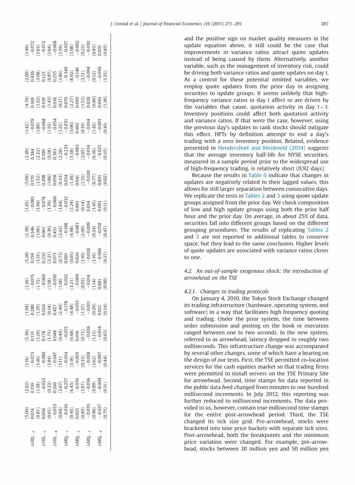
(5.00)

(2.62)

(1.16)

(5.36)

(1.94)

(1.36)

(5.28)

(2.38)

(1.45)

(5.09)

(2.49)

(1.42)

(4.74)

(2.60)

(1.49)

ΔVIX

t�2

0.07

40.15

9�0.07

30.13

10.28

0�0.07

50.15

90.34

6�0.08

50.17

00.38

4�0.07

90.16

90.43

6�0.07

2(0.81)

(1.58)

(1.46)

(1.29)

(1.59)

(1.72)

(1.51)

(1.96)

(1.94)

(1.52)

(2.22)

(1.80)

(1.52)

(3.08)

(1.63)

ΔVIX

t�3

0.05

6�0.02

3�0.08

00.17

80.02

4�0.06

90.23

20.06

1�0.07

40.20

80.10

0�0.06

80.15

90.12

3�0.07

2(0.61)

(0.23)

(1.84)

(1.75)

(0.14)

(1.58)

(2.21)

(0.36)

(1.70)

(1.86)

(0.58)

(1.55)

(1.43)

(0.87)

(1.64)

ΔVIX

t�4

�0.03

30.26

6�0.04

70.04

80.42

7�0.05

00.07

50.45

1�0.06

00.05

80.38

3�0.05

40.01

80.25

5�0.06

8(0.04)

(2.67)

(1.11)

(0.49)

(2.49)

(1.18)

(0.73)

(2.62)

(1.64)

(0.53)

(2.28)

(1.22)

(0.17)

(1.86)

(1.59)

ΔMQt�

1�0.01

6�0.25

7�0.05

4�0.01

5�0.17

8�0.03

20.001

�0.19

8�0.03

20.03

4�0.23

3�0.03

10.07

0�0.34

9�0.03

7(0.45)

(6.43)

(3.18)

(0.68)

(4.48)

(3.21)

(0.05)

(4.98)

(3.24)

(1.36)

(5.58)

(3.06)

(2.27)

(8.92)

(3.08)

ΔMQt�

20.02

5�0.07

6�0.005

0.01

6�0.05

5�0.000

0.02

6�0.08

10.001

0.04

1�0.08

30.002

0.05

0�0.14

6�0.002

(0.69)

(1.87)

(0.33)

(0.71)

(1.37)

(0.03)

(1.10)

(2.00)

(0.14)

(1.55)

(2.05)

(0.19)

(1.53)

(3.51)

(0.23)

ΔMQt�

3�0.03

5�0.03

6�0.02

8�0.02

6�0.01

1�0.01

4�0.02

8�0.009

0.01

4�0.02

0�0.01

4�0.01

40.02

8�0.004

�0.01

0(0.96)

(0.89)

(1.62)

(1.13)

(0.29)

(1.14)

(1.16)

(0.24)

(1.45)

(0.77)

(0.36)

(1.42)

(0.86)

(0.12)

(0.83)

ΔMQt�

4�0.02

7�0.004

�0.007

�0.01

40.02

10.001

�0.006

�0.01

80.001

0.001

�0.02

1�0.001

0.04

3�0.04

90.01

0(0.75)

(0.11)

(0.44)

(0.63)

(0.54)

(0.09)

(0.27)

(0.47)

(0.11)

(0.02)

(0.55)

(0.10)

(1.38)

(1.25)

(0.85)

J. Conrad et al. / Journal of Financial Economics 116 (2015) 271–291 287

and the positive sign on market quality measures in theupdate equation above, it still could be the case thatimprovements in variance ratios attract quote updatesinstead of being caused by them. Alternatively, anothervariable, such as the management of inventory risk, couldbe driving both variance ratios and quote updates on day t.As a control for these potential omitted variables, weemploy quote updates from the prior day in assigningsecurities to update groups. It seems unlikely that high-frequency variance ratios in day t affect or are driven bythe variables that cause, quotation activity in day t�1.Inventory positions could affect both quotation activityand variance ratios. If that were the case, however, usingthe previous day's updates to rank stocks should mitigatethis effect. HFTs by definition attempt to end a day'strading with a zero inventory position. Related, evidencepresented in Hendershott and Menkveld (2014) suggeststhat the average inventory half-life for NYSE securities,measured in a sample period prior to the widespread useof high-frequency trading, is relatively short (0.92 days).

Because the results in Table 6 indicate that changes inupdates are negatively related to their lagged values, thisallows for still larger separation between consecutive days.We replicate the tests in Tables 2 and 3 using quote updategroups assigned from the prior day. We check compositionof low and high update groups using both the prior halfhour and the prior day. On average, in about 25% of data,securities fall into different groups based on the differentgrouping procedures. The results of replicating Tables 2and 3 are not reported in additional tables to conservespace, but they lead to the same conclusion. Higher levelsof quote updates are associated with variance ratios closerto one.

4.2. An out-of-sample exogenous shock: the introduction ofarrowhead on the TSE

4.2.1. Changes to trading protocolsOn January 4, 2010, the Tokyo Stock Exchange changed

its trading infrastructure (hardware, operating system, andsoftware) in a way that facilitates high frequency quotingand trading. Under the prior system, the time betweenorder submission and posting on the book or executionranged between one to two seconds. In the new system,referred to as arrowhead, latency dropped to roughly twomilliseconds. This infrastructure change was accompaniedby several other changes, some of which have a bearing onthe design of our tests. First, the TSE permitted co-locationservices for the cash equities market so that trading firmswere permitted to install servers on the TSE Primary Sitefor arrowhead. Second, time stamps for data reported inthe public data feed changed fromminutes to one hundredmillisecond increments. In July 2012, this reporting wasfurther reduced to millisecond increments. The data pro-vided to us, however, contain true millisecond time stampsfor the entire post-arrowhead period. Third, the TSEchanged its tick size grid. Pre-arrowhead, stocks werebracketed into nine price buckets with separate tick sizes.Post-arrowhead, both the breakpoints and the minimumprice variation were changed. For example, pre-arrow-head, stocks between 30 million yen and 50 million yen

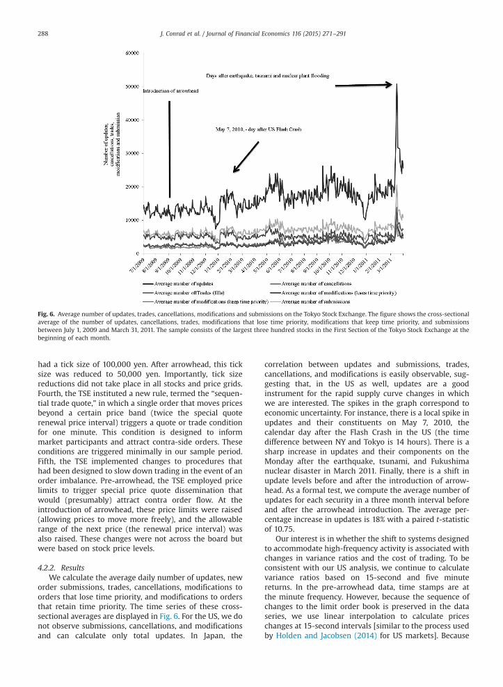
Fig. 6. Average number of updates, trades, cancellations, modifications and submissions on the Tokyo Stock Exchange. The figure shows the cross-sectionalaverage of the number of updates, cancellations, trades, modifications that lose time priority, modifications that keep time priority, and submissionsbetween July 1, 2009 and March 31, 2011. The sample consists of the largest three hundred stocks in the First Section of the Tokyo Stock Exchange at thebeginning of each month.

J. Conrad et al. / Journal of Financial Economics 116 (2015) 271–291288

had a tick size of 100,000 yen. After arrowhead, this ticksize was reduced to 50,000 yen. Importantly, tick sizereductions did not take place in all stocks and price grids.Fourth, the TSE instituted a new rule, termed the “sequen-tial trade quote,” in which a single order that moves pricesbeyond a certain price band (twice the special quoterenewal price interval) triggers a quote or trade conditionfor one minute. This condition is designed to informmarket participants and attract contra-side orders. Theseconditions are triggered minimally in our sample period.Fifth, the TSE implemented changes to procedures thathad been designed to slow down trading in the event of anorder imbalance. Pre-arrowhead, the TSE employed pricelimits to trigger special price quote dissemination thatwould (presumably) attract contra order flow. At theintroduction of arrowhead, these price limits were raised(allowing prices to move more freely), and the allowablerange of the next price (the renewal price interval) wasalso raised. These changes were not across the board butwere based on stock price levels.

4.2.2. ResultsWe calculate the average daily number of updates, new

order submissions, trades, cancellations, modifications toorders that lose time priority, and modifications to ordersthat retain time priority. The time series of these cross-sectional averages are displayed in Fig. 6. For the US, we donot observe submissions, cancellations, and modificationsand can calculate only total updates. In Japan, the

correlation between updates and submissions, trades,cancellations, and modifications is easily observable, sug-gesting that, in the US as well, updates are a goodinstrument for the rapid supply curve changes in whichwe are interested. The spikes in the graph correspond toeconomic uncertainty. For instance, there is a local spike inupdates and their constituents on May 7, 2010, thecalendar day after the Flash Crash in the US (the timedifference between NY and Tokyo is 14 hours). There is asharp increase in updates and their components on theMonday after the earthquake, tsunami, and Fukushimanuclear disaster in March 2011. Finally, there is a shift inupdate levels before and after the introduction of arrow-head. As a formal test, we compute the average number ofupdates for each security in a three month interval beforeand after the arrowhead introduction. The average per-centage increase in updates is 18% with a paired t-statisticof 10.75.

Our interest is in whether the shift to systems designedto accommodate high-frequency activity is associated withchanges in variance ratios and the cost of trading. To beconsistent with our US analysis, we continue to calculatevariance ratios based on 15-second and five minutereturns. In the pre-arrowhead data, time stamps are atthe minute frequency. However, because the sequence ofchanges to the limit order book is preserved in the dataseries, we use linear interpolation to calculate priceschanges at 15-second intervals [similar to the process usedby Holden and Jacobsen (2014) for US markets]. Because

Table 7Average paired differences in deviations of variance ratios from one,effective spreads, realized spread and price impact around the introduc-tion of arrowhead on the Tokyo Stock Exchange.

The sample consist of the 229 largest stocks on the First Section of theTokyo Stock Exchange that did not experience changes in tick size in thethree month period before and after the introduction of arrowhead. Wecalculate variance ratios over half-hour intervals based on 15-second andfive minute returns, and we compute the absolute deviation from one(|VR�1|). For each stock, we average these deviations in each half-hourinterval in the three months before and after the introduction of arrow-head, and we compute a paired difference. The column labeled|VR�1|post� |VR�1|pre shows average paired differences. We computeshare-weighted effective, realized spreads (using quote midpoints tenseconds after the trade), and price impact in each stock-day and half-hourinterval. We average these in the three months before and after theintroduction of arrowhead and report a paired difference (after minusbefore) in basis points. t-Statistics appear in parentheses.

Timeinterval

|VR�1|post� |VR�1|pre

Δ Effectivespread

Δ Realizedspread

Δ Priceimpact

9:00 to9:30 a.m.

�0.016 �1.16 �8.89 7.73(1.80) (11.12) (45.93) (39.32)

9:30 to10:00 a.m.

�0.037 �1.00 �7.81 6.80(3.18) (8.87) (39.20) (35.13)

10:00 to10:30 a.m.

�0.020 �1.01 �6.90 5.92(1.97) (7.95) (40.36) (37.58)

10:30 to11:00 a.m.

�0.015 �0.90 �6.40 5.50(1.02) (7.52) (36.35) (36.52)

12:30 to1:00 p.m.

�0.019 �2.69 �6.88 4.19(1.85) (22.68) (42.16) (22.92)

1:00 to1:30 p.m.

�0.025 �0.90 �6.18 5.29(2.25) (7.38) (37.26) (36.04)

1:30 to2:00 p.m.

�0.019 �0.89 �5.94 5.04(1.13) (7.25) (38.86) (34.29)

2:00 to2:30 p.m.

�0.027 �0.88 �5.95 5.06(1.97) (7.18) (39.41) (37.32)

2:30 to3:00 p.m.

�0.026 �1.00 �5.07 4.14(1.54) (7.56) (37.06) (39.33)

J. Conrad et al. / Journal of Financial Economics 116 (2015) 271–291 289

Fig. 6 suggests substantial changes in the informationenvironment over long periods, and because we wish tofocus purely on the effects of the arrowhead introduction,we calculate variance ratios in the three-month intervalbefore and after the introduction. We isolate securitiesthat do not experience a change in tick size so that auto-correlations (and hence variance ratios) are not affected bychanges in minimum price variation. To do so, we calculatethe minimum and maximum price level for each securityin the before and after window. We then identify securitiesthat ex post remained in the same tick size price grid. Forsuch paired comparisons, the sample consists of 229securities.

For each security, we calculate the deviation in varianceratios from one (|VR�1|) and average over the three monthpre- or post-arrowhead period for each half hour of trading.We then compute paired differences between the pre- andpost-period averages for each security. The second column ofTable 7 shows the cross-sectional average of these paireddifferences, along with their t-statistics. In every half hour ofthe trading day, the change in the deviations of variance ratiosfrom one is negative, implying an improvement in varianceratios. The magnitude of the changes in average variance ratiosranges from 0.01 to 0.03, similar to the differences betweenhigh update and low update groups in the US (Table 3).

We also calculate share-weighted effective spreads foreach stock, again restricting the sample to securities withno changes in tick size. Average paired changes in effectivespreads are in the third column of Table 7. In each halfhour interval, effective spreads decline by approximately 1and 2 basis points. The largest decline is in the first halfhour in the afternoon trading session, at 2.69 basis points.All changes are highly statistically significant. Because pre-arrowhead effective spreads are approximately 10 basispoints, a decline of between 1 to 2 basis points iseconomically large.

As with US data, we compute realized spreads andprice impact using a variety of horizons but show only onehorizon (ten seconds) for brevity. The fourth and fifthcolumns of the table show changes in realized spreads andprice impact based on midpoints ten seconds after a trade.The results show a substantial decline in the realizedspread, varying from 5 to almost 9 basis points, and anincrease in price impact, varying from 4 to approximately8 basis points. Fig. 7 shows that the changes occur sharplyat the introduction of arrowhead. The relation betweeneffective spreads, realized spreads, and price impact ismechanical. If effective spreads decline by about 1–2 basispoints and realized spreads decline by a larger amount, itmust be the case that price impact increases.

The increase in price impact associated in this market isnot consistent with the decline in price impact after autoquotein the US market, observed in Hendershott, Jones, andMenkveld (2011). We speculate that this difference is relatedto different rules on price continuity in the two markets. Priorto arrowhead, the TSE's trading protocols smoothed pricepaths when an order imbalance occurred. In effect, changes inspread midpoints were suppressed, reducing measured priceimpacts. Post-arrowhead, the magnitude of the smoothing issubstantially reduced, which would present itself as anincrease in price impact. To test this conjecture, we calculatethe frequency of special price quote dissemination before andafter the introduction of arrowhead. We do so for each stockin the three-month interval before and after arrowhead andfind that special quote dissemination decreases by an averageof 50% (t-statistic¼12.72) following arrowhead introduction.To further test whether differences in special quote dissemi-nation influence the measures of price impact, we separate allstocks (without tick size changes) into two groups based onwhether the percentage increase in special quote dissemina-tion is above or below the median. In each half-hour interval,the increase in price impact following the introduction ofarrowhead is significantly higher (by between 1 and 2 basispoints) for stocks which experienced a larger decline in specialquote dissemination following arrowhead.

Summarizing, the introduction of arrowhead trading wasdesigned to reduce the latency of trading on the TSE. Followingits introduction, variance ratios move closer to one. Themagnitude of this change is very similar to the difference invariance ratios observed in high update and low update groupsin the US. Effective spreads also decline sharply immediatelyaround the shift to arrowhead, with the magnitude of thisdecline roughly similar to the difference in effective spreads inhigh and low update groups in the US. Overall, the exogenouschange in trading platforms in Japan confirms the evidencefrom US equity markets, that higher levels of high-frequency

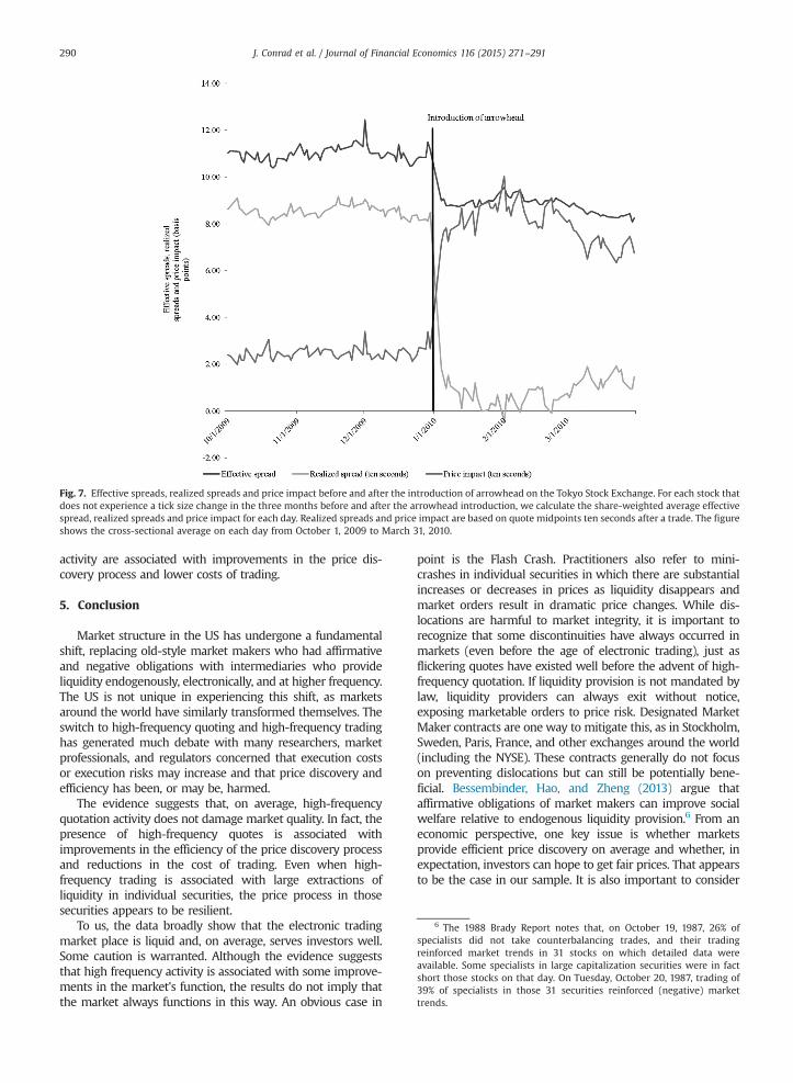
Fig. 7. Effective spreads, realized spreads and price impact before and after the introduction of arrowhead on the Tokyo Stock Exchange. For each stock thatdoes not experience a tick size change in the three months before and after the arrowhead introduction, we calculate the share-weighted average effectivespread, realized spreads and price impact for each day. Realized spreads and price impact are based on quote midpoints ten seconds after a trade. The figureshows the cross-sectional average on each day from October 1, 2009 to March 31, 2010.

6 The 1988 Brady Report notes that, on October 19, 1987, 26% ofspecialists did not take counterbalancing trades, and their tradingreinforced market trends in 31 stocks on which detailed data wereavailable. Some specialists in large capitalization securities were in factshort those stocks on that day. On Tuesday, October 20, 1987, trading of39% of specialists in those 31 securities reinforced (negative) markettrends.

J. Conrad et al. / Journal of Financial Economics 116 (2015) 271–291290

activity are associated with improvements in the price dis-covery process and lower costs of trading.

5. Conclusion

Market structure in the US has undergone a fundamentalshift, replacing old-style market makers who had affirmativeand negative obligations with intermediaries who provideliquidity endogenously, electronically, and at higher frequency.The US is not unique in experiencing this shift, as marketsaround the world have similarly transformed themselves. Theswitch to high-frequency quoting and high-frequency tradinghas generated much debate with many researchers, marketprofessionals, and regulators concerned that execution costsor execution risks may increase and that price discovery andefficiency has been, or may be, harmed.

The evidence suggests that, on average, high-frequencyquotation activity does not damage market quality. In fact, thepresence of high-frequency quotes is associated withimprovements in the efficiency of the price discovery processand reductions in the cost of trading. Even when high-frequency trading is associated with large extractions ofliquidity in individual securities, the price process in thosesecurities appears to be resilient.

To us, the data broadly show that the electronic tradingmarket place is liquid and, on average, serves investors well.Some caution is warranted. Although the evidence suggeststhat high frequency activity is associated with some improve-ments in the market's function, the results do not imply thatthe market always functions in this way. An obvious case in

point is the Flash Crash. Practitioners also refer to mini-crashes in individual securities in which there are substantialincreases or decreases in prices as liquidity disappears andmarket orders result in dramatic price changes. While dis-locations are harmful to market integrity, it is important torecognize that some discontinuities have always occurred inmarkets (even before the age of electronic trading), just asflickering quotes have existed well before the advent of high-frequency quotation. If liquidity provision is not mandated bylaw, liquidity providers can always exit without notice,exposing marketable orders to price risk. Designated MarketMaker contracts are one way to mitigate this, as in Stockholm,Sweden, Paris, France, and other exchanges around the world(including the NYSE). These contracts generally do not focuson preventing dislocations but can still be potentially bene-ficial. Bessembinder, Hao, and Zheng (2013) argue thataffirmative obligations of market makers can improve socialwelfare relative to endogenous liquidity provision.6 From aneconomic perspective, one key issue is whether marketsprovide efficient price discovery on average and whether, inexpectation, investors can hope to get fair prices. That appearsto be the case in our sample. It is also important to consider

J. Conrad et al. / Journal of Financial Economics 116 (2015) 271–291 291

whether a particular market structure increases or decreasesthe propensity for dislocations to occur, as well as how itaffects the severity of the dislocation. The effects of recentregulatory changes to the market structure on market volati-lity, and the propensity of dislocations to occur, is the subjectof our current research.

Caution is also warranted given potential externalitiesthat we cannot measure. A trade-off exists between the costand benefit of monitoring high-frequency quotation activity(Foucault, Roëll, and Sandas, 2003; Foucault, Kadan, andKandel, 2013). If liquidity suppliers change supply curves inmicroseconds and liquidity extractors bear the cost ofmonitoring supply curves, then this can have a negativeeffect on welfare. We provide no evidence on the extent towhich high-frequency quotation/trading affects welfare.However, understanding the influence of rapidly changingsupply curves on price formation and the cost of trading isnevertheless important because, as Stiglitz (2014) pointsout, these are intermediate variables that are necessary(although not sufficient) for understanding the role of high-frequency quoting and trading on welfare.

References

Aϊt-Sahalia, Y., Saglam, M., 2013. High-frequency traders: taking advan-tage of speed. Unpublished working paper. National Bureau ofEconomic Research, Cambridge, MA.

Baruch, S., Glosten, L., 2013. Fleeting orders. Unpublished working paper.Columbia University, New York, NY.

Bessembinder, H., Hao, J., Zheng, K., 2013. Market making obligations andfirm value. Unpublished working paper. University of Utah, Salt LakeCity, UT.

Biais, B., Foucault, T., Moinas, S., 2014. Equilibrium fast trading. Unpub-lished working paper. Toulouse School of Economics, Toulouse,France.

Brogaard, J., Hendershott, T., Riordan, R., 2014. High-frequency tradingand price discovery. Review of Financial Studies 27 (8), 2267–2306.

Brunnermeier, M., Pedersen, L., 2009. Market liquidity and fundingliquidity. Review of Financial Studies 22, 2201–2238.

Budish, E., Cramton, P., Shim, J., 2013. The high-frequency trading armsrace: frequent batch auctions as a market design response. Unpub-lished working paper. University of Chicago, Chicago, IL.

Campbell, J., Lo, A., MacKinlay, A., 1997. In: The Econometrics of FinancialMarketsPrinceton University Press, Princeton, NJ.

Carrion, A., 2013. Very fast money: high frequency trading on the Nasdaq.Journal of Financial Markets 16, 680–711.

Foucault, T., Roëll, A., Sandas, P., 2003. Market making with costlymonitoring: an analysis of the SOES controversy. Review of FinancialStudies 16, 345–384.

Foucault, T, Kadan, O., Kandel, E., 2013. Liquidity cycles and make/takefees in electronic markets. Journal of Finance 68 (1), 299–341.

Hagströmer, B., Norden, L., 2013. The diversity of high-frequency traders.Journal of Financial Markets 16, 741–770.

Han, J., Khapko, M., Kyle, A., 2014. Liquidity with high frequency marketmaking. Unpublished working paper. University of Maryland, CollegePark, MD.

Hasbrouck, J., 2013. High-frequency quoting: short-term volatility in bidsand offers. Unpublished working paper. New York University, NewYork, NY.

Hendershott, T., Menkveld, A., 2014. Price pressures. Journal of FinancialEconomics 114, 405–423.

Hendershott, T., Jones, C., Menkveld, A., 2011. Does algorithmic tradingimprove liquidity? Journal of Finance 66, 1–33.

Hirshey, N., 2013. Do high-frequency traders anticipate buying and sellingpressure. Unpublished working paper. London Business School,London, UK.

Holden, C., Jacobsen, S., 2014. Liquidity measurement problems in fastcompetitive markets: expensive and cheap solutions. Journal ofFinance 69, 1747–1785.

Lo, A., MacKinlay, A., 1988. Stock prices do not follow random walks:evidence from a simple specification test. Review of Financial Studies1, 41–66.

Lo, A., MacKinlay, A., 1989. The size and power of the variance ratio test infinite samples: a Monte Carlo investigation. Journal of Econometrics40, 203–238.

Madhavan, A., Cheng, M., 1997. In search of liquidity: block trades in theupstairs and downstairs markets. Review of Financial Studies 10,175–203.

Menkveld, A., 2012. High-frequency traders and the new market makers.Unpublished working paper. VU University Amsterdam, Amsterdam,Netherlands.

Nagel, S., 2012. Evaporating liquidity. Review of Financial Studies 25,2005–2039.

Riordan, R., Storkenmaier, A., 2012. Latency, liquidity and price discovery.Journal of Financial Markets 15, 416–437.

Stiglitz, J., 2014. Tapping the brakes: are less active markets safer andbetter for the economy? Unpublished working paper. ColumbiaUniversity, New York, NY.