reconstructing the unknown local volatility …janroman.dhis.org/finance/volatility models/local...

RECONSTRUCTING THE UNKNOWN LOCAL VOLATILITY FUNCTION

THOMAS F. COLEMAN∗, YUYING LI∗, AND ARUN VERMA∗

Abstract. Using market European option prices, a method for computing a smooth local volatility function in

a 1-factor continuous diffusion model is proposed. Smoothness is introduced to facilitate accurate approximation

of the local volatility function from a finite set of observation data. Assuming that the underlying indeed follows

a 1-factor model, it is emphasized that accurately approximating the local volatility function prescribing the 1-

factor model is crucial in hedging even simple European options, and pricing exotic options. A spline functional

approach is used: the local volatility function is represented by a spline whose values at chosen knots are de-

termined by solving a constrained nonlinear optimization problem. The optimization formulation is amenable to

various option evaluation methods; a partial differential equation implementation is discussed. Using a synthetic

European call option example, we illustrate the capability of the proposed method in reconstructing the unknown

local volatility function. Accuracy of pricing and hedging is also illustrated. Moreover, it is demonstrated that,

using different implied volatilities for options with different strikes/maturities can produce erroneous hedge fac-

tors if the underlying follows a 1-factor model. In addition, real market European call option data on the S&P 500

stock index is used to compute the local volatility function; stability of the approach is demonstrated.

∗ Computer Science Department and Cornell Theory Center, Cornell University, Ithaca, NY 14850. Research

partially supported by the Applied Mathematical Sciences Research Program (KC-04-02) of the Office of Energy

Research of the U.S. Department of Energy under grant DE-FG02-90ER25013.A000 and NSF through grant

DMS-9505155 and ONR through grant N00014-96-1-0050.

This research was conducted using resources of the Cornell Theory Center, which is supported by Cornell

University, New York State, the National Center for Research Resources at the National Institutes of Health, and

members of the Corporate Partnership Program.

0

1. Introduction. An option pricing model establishes a relationship between the traded

derivatives, the underlying asset and the market variables, e.g., volatility of the underlying

asset [4, 25]. Option pricing models are used in practice to price derivative securities given

knowledge of the volatility and other market variables.

The celebrated constant-volatility Black-Scholes model [4, 25] is the most often used

option pricing model in financial practice. This classical model assumes constant volatility;

however, much recent evidence suggests that a constant volatility model is not adequate [27,

28]. Indeed, numerically inverting the Black-Scholes formula on real data sets supports the

notion of asymmetry with stock price (volatility skew), as well as dependence on time to

expiration (volatility term structure). Collectively this dependence is often referred to as the

volatility smile. The challenge is to accurately (and efficiently) model this volatility smile.

In practice, the constant-volatility Black-Scholes model is often applied by simply using

different volatility values for options with different strikes and maturities. In this paper, we

refer to this approach as the constant implied volatility approach. Although this method works

well for pricing European options, it is unsuitable for more complicated exotic options and

options with early exercise features. Moreover, as will be illustrated in §4, this approach

can produce incorrect hedge factors even for simple European options, assuming that the

underlying follows a 1-factor model.

A few different approaches have been proposed for modeling the volatility smile. One

class of methods (Merton [26]) assumes a Poisson jump diffusion process for the underly-

ing asset. Stochastic volatility models (Hull and White [20]) have also been used. Das and

Sundaram [10] indicate that neither of these types of models sufficiently explains the implied

volatility structure.

Finally, there is the 1-factor continuous diffusion approach: an underlying asset with the

initial value Sinit is assumed to satisfy:

dSt

St= µ(St, t)dt + σ∗(St, t)dWt, t ∈ [0, τ ], τ > 0,(1)

where Wt is a standard Brownian motion, τ is a fixed trading horizon, and µ, σ ∗: �+ ×[0, τ ] → � are deterministic functions. The function σ ∗(s, t) is called the local volatility

function. The advantages of the 1-factor continuous diffusion model, compared to the jump

or stochastic model, include that no non-traded source of risk such as the jump or stochastic

volatility is introduced [17]. Consequently, the completeness of the model, i.e., the ability to

1

hedge options with the underlying asset, is maintained. Completeness is ultimately important

since it allows for arbitrage pricing and hedging [17].

There may be dispute regarding whether a 1-factor model (1) is the best way to model an

underlying process. Our research will not shed light to this dispute. Instead, we demonstrate

the importance of accurately approximating the local volatility function in pricing and hedging

derivatives when the underlying follows a 1-factor model (1).

In order to price complex exotic options using a 1-factor diffusion model (1), the volatil-

ity function σ∗(s, t) needs to be approximated. Volatility is the only variable in this 1-factor

model which is not directly observable in the market. Similar to the implied volatility in the

constant volatility model, one possible idea is to imply this local volatility function from the

market option price data. Indeed, it is established [1, 17] that the local volatility function can

be uniquely determined from the European call options of all strikes and maturities, under

the no arbitrage assumption of the observable European call option prices. Unfortunately, the

market European option prices are typically limited to a relatively few different strikes and

maturities. Therefore the problem of determining the local volatility function can be regarded

as a function approximation problem from a finite data set with a nonlinear observation func-

tional. Due to insufficient market option price data, this is a well-known ill-posed problem.

Computational methods have been proposed to solve this ill-posed problem [1, 2, 5, 13,

14, 17, 22, 23, 27]. Most of these methods [1, 5, 13, 14, 17, 22, 27] overcome the ill-posedness

of the problem by assuming the existence of a complete spanning set of European call option

prices, which, in practice, requires use of extrapolation and interpolation of the available

market option prices [5, 13, 22, 27]. This can be problematic because potentially erroneous

non-market information are introduced into the data. Rubinstein proposes to compute the

implied probability without any exogenous assumption on the model for the local volatility

function [22, 27]. In [1] the local volatility is computed at each discretization nodal point

with a PDE approach. The methods [2, 23] use a regularization approach to the ill-posed local

volatility approximation problem. The closeness of the local volatility to a prior is used in [2]

and smoothness is used in [23].

The local volatility function approximation problem is ill-posed: there are typically an

infinite number of solutions to the problem. It is not difficult to find a local volatility function

σ(s, t) that matches the market option price data. However, for accurately pricing exotic

options, we are not merely concerned with matching the market option prices but would like

2

to reconstruct as accurately as possible the volatility function σ ∗(s, t) in the diffusion model

(1). Accurately approximating this volatility function is especially important for computing

hedge factors, even for simple European call/put options, see §4.

Smoothness of the function has long been used as a regularization criterion for function

approximation with a finite observation data [29, 30, 31]. Splines have known to possess good

approximation theoretical properties for a model both when the function is fixed and smooth

and when it is a sample function from a stochastic process [31]. However, approximating

the local volatility function from a finite set of option prices is more complex, compared to

a standard function approximation problem, since the (observation) option price functional is

nonlinear. Nevertheless, it is intuitive that smoothness regularization will play a similar role

here.

In [23] the lack of sufficient market option price data is overcome by regularizing with

smoothness of the local volatility function. The local volatility is computed at each discretiza-

tion point to match the given option prices with an additional objective of minimizing the

change of the derivative ∇σ(s, t). Unfortunately, this approach requires the solution of a very

large-scale nonlinear optimization problem: the dimension is equal to the total number of

discretization points. In addition, it requires determination of a regularization parameter.

In this paper, we propose a spline functional approach: a local volatility function σ(s, t)

is explicitly represented by a spline with a fixed set of spline knots and end condition. The

volatilities at the spline knots uniquely determine a local volatility function. We choose the

number of spline knots to be no greater than the number of option prices and they are placed

with respect to the given data. The spline is determined by solving a constrained nonlinear

optimization problem to match the market option prices as closely as possible. The dimen-

sion of the optimization problem is typically small, depending on the number of option prices

available. The approximation properties of the spline allow an accurate and smooth approxi-

mation of the local volatility function prescribing the 1-factor model in a region within which

the volatility values are significant for pricing available options.

We start with the motivation for our proposed inverse spline approximation formulation

for the local volatility in §2. Computational issues for solving the proposed optimization

problem are discussed in §3. Numerical examples illustrating the reconstructed local volatil-

ity surfaces from the European call option prices are described in §4. Using a European call

option example with the underlying following the known absolute diffusion process, we illus-

3

trate the capability of the proposed method for accurately reconstructing the local volatility

function. A S&P 500 European index call option example with the real market data is also

used to illustrate the smoothness of the local volatility function and the stability of the pro-

posed approach. In §5, concluding remarks are given.

2. Local Volatility Function Approximation with Splines. Assume that the underly-

ing asset follows a continuous 1-factor diffusion process with the initial value S init:

dSt

St= µ(St, t)dt + σ∗(St, t)dWt, t ∈ [0, τ ],

for some fixed time horizon [0, τ ], Wt is a Brownian motion, and µ(s, t), σ∗(s, t): �+ ×[0, τ ] → � are deterministic functions sufficiently well behaved to guarantee that (1) has a

unique solution [24]. Note that in this notation σ ∗(s, t) can be negative as well as positive.

(The conventional notion of positive volatility corresponds to√

σ∗(s, t)2 in our notation.) For

simplicity, we assume that the instantaneous interest rate is a constant r > 0 and the dividend

rate is a constant q > 0 (A general stochastic interest derivative pricing can be priced, e.g.,

[19]). Given Sinit, r and q, and under the no arbitrage assumption [25], an option with the

volatility σ(s, t), strike price K, and maturity T has a unique price v(σ(s, t), K, T ).

Assume that we are given m market option (bid,ask)-pairs, {(bidj, askj)}mj=1, corre-

sponding to strike prices/expiration times {(K j, Tj)}mj=1. Let

vj(σ(s, t)) def= v(σ(s, t), Kj, Tj), j = 1, · · · , m.

We want to approximate, as accurately as possible, the local volatility function σ ∗(s, t) :

�+ × [0, τ ] → � from the requirement that

bidj ≤ vj(σ(s, t)) ≤ askj, j = 1, · · · , m.(2)

Since the observation data {(bidj, askj, Kj, Tj)}mj=1 is finite and the restriction is on the op-

tion values {vj(σ(s, t))}mj=1, problem (2) can be considered an inverse function approximation

problem from a finite observation data. Let H denote the space of measurable functions in the

region [0, +∞)× [0, τ ]. The inverse function approximation problem (2) can be written as an

optimization problem:

minσ(s,t)∈H

m∑j=1

[bidj − vj(σ(s, t)))]+ +m∑

j=1

[vj(σ(s, t))− askj)]+,(3)

4

where x+ def= max(x, 0). This is a nonlinear piecewise differentiable optimization problem:

to overcome nondifferentiability in (3), one can alternatively solve a variational least squares

problem:

minσ(s,t)∈H

m∑j=1

(vj(σ(s, t))− vj)2,(4)

where vjdef= bidj+askj

2 . Since the observation data is finite, problems (2,3,4) are severely

underdetermined: there are typically an infinite number of solutions. It is easy to find a

function σ(s, t) that matches the market option price data [2, 5, 17, 13, 14, 22, 23, 27].

The local volatility reconstruction problem (2,3,4) is a complicated nonstandard function

approximation problem. The option price functional v(σ(s, t), K, T ) is nonlinear in the local

volatility function σ(s, t). It is a nonlinear inverse function approximation problem.

In most of the proposed methods [1, 2, 5, 17, 13, 14, 22, 27] matching the market option

price data has been emphasized; it is often the only objective. However, a function σ(s, t)

which matches the finite set of market option prices can be very different from the local

volatility σ∗(s, t) which prescribes the 1-factor model for the underlying, see §4 for an exam-

ple. Moreover, the price vj generally has error (for example when a bid-ask spread exists). In

addition, the option value v j(σ(s, t)) can only be computed numerically using a tree method

or a PDE approach (there is no closed form solution for a general 1-factor model (1)). Hence,

it may not be desirable to insist that v j(σ(s, t)) match exactly the observed market price vj

for j = 1, · · · , m. For pricing and hedging of exotic options, it is more important to compute

a local volatility function σ(s, t) which is as close as possible to the local volatility function

σ∗(s, t). In other words, in addition to calibrating the market option price data sufficiently ac-

curately, we would like to reconstruct, as accurately as possible, the local volatility function

σ∗(s, t) of the diffusion model (1).

Smoothness has long been used [29, 30, 31] as a regularization condition for a function

approximation problem with a limited observation data. In addition, smoothness of the local

volatility function can be important in computational option valuation schemes. Convergence

of a PDE finite difference method, for example, depends on the smoothness of the function

σ(s, t).

In [23] it is proposed to use smoothness as a regularization condition to approximate the

5

local volatility function. The regularized optimization problem

minσ(s,t)∈H

m∑j=1

(vj(σ(s, t)))− vj)2 + λ‖∇σ(s, t)‖2(5)

is used in [23] where λ is a positive constant and ‖ · ‖ 2 denotes the L2 norm. The change of

the first order derivative is minimized depending on the regularization parameter λ for which

determining a suitable value may not be easy. In addition, computational implementation

of this method requires solving a large-scale discretized optimization problem: for a PDE

implementation, the dimension is NM where N is the number of discretization points in s

and M is the number of discretization points in t. A simple gradient descent algorithm is

used in [23]. Since the optimization problem is (5) highly nonlinear, with such a method, the

computed solution is typically inaccurate. To use a more sophisticated optimization algorithm,

the Jacobian matrix of the vector function (v1, · · · , vm) needs to be evaluated but this becomes

extremely costly due to the large dimension of the discretized problem.

Splines have long been used in approximating smooth curves and surfaces (see, e.g.,

[16]). They have also been used as a tool for regularizing ill-posedness of function approx-

imations from finite observation data [31]. In a typical 1-dimensional spline interpolation

setting, assuming values fi, i = 1, · · · , m, of the dependent variable f(x) corresponding to

values xi, i = 1, · · · , m, are given, a spline is chosen to fit the data (f i, xi), i = 1, · · · , m.

Given the number of knots p and their locations, the freedom of the spline is the coefficient of

each spline segment. The cubic spline has long been used by craftsman and engineers as the

mechanic spline. It is the smoothest twice continuously differentiable function that matches

the observations; the minimizer of

minf(x)∈S

∫ b

a(f ′′(x))2dx, subject to f(xi) = fi, i = 1, · · · , m,

is a natural cubic spline, where S is the Sobolev space of functions whose first order deriva-

tives are continuously differentiable and the second order derivatives are square integrable

(assuming m ≥ 2). For mechanical splines, this corresponds to minimize the elastic strain

energy. For 2-dimensional surface fitting, the bicubic spline defined on a regular grid is twice

continuously differentiable [3, 16]. The bicubic spline has a similar variational minimization

property. Advantages of spline interpolation include its fast convergence on many types of

meshes, computational efficiency, and insensitivity to roundoff errors [3].

Approximating the local volatility function by a spline is particularly reasonable if the

local volatility function is smooth. Is this a reasonable expectation for the local volatility

6

function? Assume that the underlying follows the 1-factor diffusion process (1). Let there

be given observable arbitrage-free market European call prices v(K, T ) for all strikes K ∈[0,∞) and all maturities T ∈ (0, τ ]. From Proposition 1 in [1], the local volatility function

σ∗(s, t) of the diffusion process (1) that is consistent with the market is given uniquely by

(σ∗(K, T ))2 = 2∂v∂T + qv(K, T ) + K(r − q) ∂v

∂K

K2 ∂2v∂K2

.(6)

This formula suggests that, assuming v(K, T ) is sufficiently smooth (note that ∂2v∂K2 and ∂v

∂T

already exist) and ∂2v∂K2 = 0, (σ∗(K, T ))2 is sufficiently smooth in the region (0,∞) × (0, τ ]

as well.

In this paper, we use a 2-dimensional spline functional to directly approximate a local

volatility function1. Let the number of spline knots p ≤ m. We choose a set of fixed spline

knots {(sj, tj)}pj=1 in the region [0,∞) × [0, τ ]. Given {(si, ti)}p

i=1 spline knots with cor-

responding local volatility values σ idef= σ(si, ti), an interpolating cubic spline c(s, t) with a

fixed end condition (in our computation the natural spline end condition is used) is uniquely

defined by setting c(si, ti) = σi, i = 1, · · · , p. We then determine the local volatility values

σi (hence the spline) by calibrating the market observable option prices. The freedom in this

problem is represented by the volatility values {σ i} at the given knots {(si, ti)}. If σ is a

p-vector, σ = (σ1, · · · , σp)T , then we denote the corresponding interpolating spline with the

specified end condition as c(s, t; σ).

Let

vj(c(s, t; σ)) def= v(c(s, t; σ), Kj, Tj), j = 1, · · · , m.

To allow the possibility of incorporating additional a priori information, l and u are lower and

upper bounds that can be imposed on the local volatilities at the knots. Thus, we define the in-

verse spline local volatility approximation problem: Given p spline knots, (s 1, t1) · · · , (sp, tp),

solve for the p-vector σ

minσ∈�p

f(σ) def=12

m∑j=1

wj[vj(c(s, t; σ))− vj]2

subject to l ≤ σ ≤ u,(7)

where positive constants {wj}mj=1 are weights, allowing account to be taken of different ac-

curacies of vj or computed vj . The determination of an approximation in the l1 or l∞ norm

1 If it is known that σ(s, t) is a function of s or t only, then one can use 1-dimensional spline.

7

instead may be a valuable alternative although the problem becomes even more difficult to

solve computationally. Note also that the formulation (7) is quite general: European call/put

or even more complicated option prices can be used to compute the spline approximation to

the local volatility function σ ∗(s, t).

The inverse spline local volatility problem (7) is a minimization problem with respect to

the local volatility σ at the spline knots. The computed volatility function has some depen-

dence on the number of knots p and the location of the knots {(s i, ti)}pi=1. The choice of the

number of knots and their placement in spline approximation is generally a complicated issue

[16, 31]. The situation here is not typical for spline approximation due to the fact that the

dependent option price function is not the function to be approximated. Rather, it depends

on the values of the unknown volatility function in the region R + × [0, τ ]. Moreover, the

dependence on the unknown volatility values is not uniform in the region R + × [0, τ ]. The

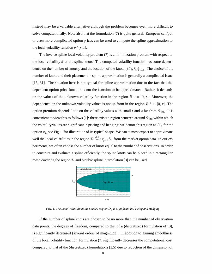
option premium depends little on the volatility values with small t and s far from S init. It is

convenient to view this as follows [1]: there exists a region centered around S init within which

the volatility values are significant in pricing and hedging: we denote this region as D j for the

option vj , see Fig. 1 for illustration of its typical shape. We can at most expect to approximate

well the local volatilities in the region D def= ∪mj=1Dj from the market option data. In our ex-

periments, we often choose the number of knots equal to the number of observations. In order

to construct and evaluate a spline efficiently, the spline knots can be placed in a rectangular

mesh covering the region D and bicubic spline interpolation [3] can be used.

Significant

Insignificant

Time t

Sinit

jT

K j

FIG. 1. The Local Volatility in the Shaded Region D j Is Significant in Pricing and Hedging

If the number of spline knots are chosen to be no more than the number of observation

data points, the degrees of freedom, compared to that of a (discretized) formulation of (3),

is significantly decreased (several orders of magnitude). In addition to gaining smoothness

of the local volatility function, formulation (7) significantly decreases the computational cost

compared to that of the (discretized) formulations (3,5) due to reduction of the dimension of

8

the optimization problem.

It is not appropriate to choose p much larger than m since (7) may become underdeter-

mined. If one decides to use more spline knots, additional regularization, e.g.,

minσ∈�p

f(σ) def=12

m∑j=1

wj[vj(c(s, t; σ)) − vj ]2 + λη(c(s, t; σ))

subject to l ≤ σ ≤ u,(8)

is more appropriate: here λ > 0 is a regularization parameter and η(σ(s, t; σ)) is a smoothing

norm for the tensor product splines [15]. (A referee has pointed out that this has recently been

considered in [21].)

In this paper, we focus on the formulation (7) and assume p is not greater than m. In

order to solve the inverse local volatility problem (7), an optimization method will be needed

to evaluate the values of options v j(c(s, t; σ)) for any spline c(s, t; σ); the derivatives may

also be computed. We discuss this next.

3. The Computational Procedure. Our proposal is to approximate the local volatility

surface, σ∗(s, t), with a cubic spline c(s, t; σ) by solving (7) for the vector σ = (σ 1, · · · , σp)T .

Problem (7), when p ≤ m, is defined once the p knots (s1, t1), · · · , (sp, tp) have been chosen

appropriately. To express (7) more succinctly, define a vector-valued function F : � p → �m

where component j of F is given by w12j [vj(c(s, t; σ))− vj], for j = 1, · · · , m. Therefore (7)

can be rewritten:

minσ∈�p

f(σ) def=12‖F (σ)‖2

2

subject to l ≤ σ ≤ u.(9)

Problem (9) is a box-constrained nonlinear least-squares problem in σ; there are a vari-

ety of optimization methods available to enable its solution. In our implementation we use

a trust region/interior point method [6, 7], in which a sequence of strictly feasible points

are generated: {σ(k)} ∈ int{F}, where F = {σ ∈ �p : l ≤ σ ≤ u}. Moreover,

the sequence corresponds to a monotonically decreasing sequence of function values, i.e.,

f (k+1) < f (k), k = 1, · · · ,∞, where f (k) = f(σ(k)). Under mild assumptions this approach

guarantees convergence, i.e., σ(k) → σ∗, where σ∗is a local minimizer for problem (9).

The Jacobian of F with respect to σ is required: J(σ) def= ∇F (σ). Note that J is an

m×p matrix. In the square case when p = m, it is possible to use a standard secant update to

9

approximate J , e.g., [12], which can significantly reduce the cost. Under reasonable assump-

tions a superlinear rate of convergence can be achieved. We note that there are optimization

approaches that do not require the calculation (or approximation) of the Jacobian matrix J;

however, they typically converge very slowly - we have not investigated those methods in this

work.

In this paper we explore two possibilities in the framework of our optimization approach:

1. Use of automatic differentiation [8] and/or finite-differencing to compute J (k) def=

J(σ(k));

2. Use of a secant update to approximate J (k) when p = m.

3.1. The Problem Structure. The evaluation of f(σ) requires the evaluation of each

component of F , i.e., w12j [vj(c(s, t); σ)− vj], for j = 1, · · · , m. These are generalized Black-

Scholes computations. There are several ways to approach this – we choose, as an example,

to use a standard PDE-discretization technique.

Given Sinit, r, q, and σ(s, t), let V (s, t) denote the option value of an underlying asset

with strike price K and expiry date T at (s, t), t ∈ [0, T ]. Under the no arbitrage assumption,

the option value satisfies the following generalized Black-Scholes equation [25]

∂V

∂t+ (r − q)s

∂V

∂s+

12σ(s, t)2s2 ∂2V

∂s2= rV.(10)

The boundary conditions for the European call option are :

lims→+∞

∂V (s, t)∂s

= e−q(T−t), t ∈ [0, T ],

V (0, t) = 0, t ∈ [0, T ],

V (s, T ) = max(s − K, 0).

We use a Crank-Nicholson finite difference solution strategy for solving (10), based on

discretization on a uniform grid. Given a 2-dimensional grid the numerical solution of (10) is

standard and discussed in several texts. Zvan et al [32] have a good discussion of complexity

issues. It is possible to increase efficiency by employing a number of computing techniques

such as vectorization and pipelining – description of these implementation aspects goes be-

yond the scope of this paper.

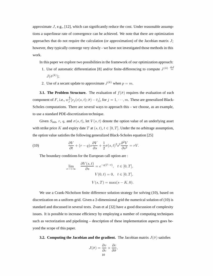
3.2. Computing the Jacobian and the gradient. The Jacobian matrix J(σ) satisfies

J(σ) =∂v

∂c× ∂c

∂σ,

10

where ∂v∂c is an m-by-MN matrix, ∂c

∂σ is an MN -by-p matrix.

It is useful to note that matrix Cdef= ∂c

∂σ is constant and therefore needs to be computed

just once for the entire problem (given a fixed discretization and spline knot placement). The

product ∂v∂c × C can be computed directly using automatic differentiation (forward mode)

or approximately using finite differences (differencing v along the columns of C). In either

case the work involved is O(p · ω(F )) where ω(F ) is the work (flops) required to evaluate

F . (In the finite-differencing case this is a tight bound whereas this bound can be undercut

considerably if automatic differentiation is used [18].)

The gradient of f , with respect to σ, is simply J T F . Therefore if the function F and its

Jacobian J have been computed as described above the gradient is given by a matrix-vector

multiplication.

If the secant method is used in the square case, i.e., p = m, then the gradient is approx-

imated by A × F where A is the secant approximation to the Jacobian. The Jacobian is not

computed (except, possibly, for secant method restarts) with this approach.

4. Computational Examples. We now describe some computational experience with

our proposed method for reconstructing the local volatility function σ ∗(s, t) from limited

observation data. We illustrate how European call options can be used to approximate the

local volatility function.

We have implemented the proposed method in Matlab using a trust region optimiza-

tion algorithm with a PDE approach for function and Jacobian evaluation. Without precise

knowledge of accuracy of the market data, the weights in the inverse spline local volatility

approximation problem (7) are simply set to unity: w jdef= 1, j = 1, · · · , m. The generalized

Black-Scholes PDE (10) is solved with a Crank-Nicolson finite difference method. Given any

σ, the bicubic spline c(s, t; σ) with the variational end condition (the second order derivative

at the end is zero) is computed and evaluated using the functions in the Matlab spline toolbox

[11]. We use a simple discretization scheme: a uniformly spaced mesh with N × M grid

points in the region [0, 2S init] × [0, τ ] where τ is the maximum maturity in the market option

data:

si = i2SinitN−1 , i = 0, · · · , N − 1,

tj = j τM−1 , j = 0, · · · , M − 1.

(11)

For simplicity, we have chosen the spline knots to be on a uniform rectangular mesh cov-

ering the region D in which the volatility values are significant in pricing the market options.

11

Given a European option, we do not have an explicit knowledge of the region D. In our ex-

periments, we have used [γ1Sinit, γ2Sinit] × [0, τ ] as an estimate of D with γ1 ∈ [.6, .8] and

γ2 ∈ [1.4, 1.6] depending on the magnitude of S init. The number of spline knots p typically

equals the number of observation m. In the event that the option prices are calibrated to high

precision, we have experimented with p < m.

4.1. Reconstructing Local Volatility, Pricing and Hedging. In order to demonstrate

the effectiveness of the proposed method in reconstructing the local volatility surface and its

accuracy in pricing and hedging, we consider a synthetic European call option example used

in [23]. In this example, the underlying is assumed to follow an absolute diffusion process:

dSt

St= µ(St, t)dt + σ∗(St, t)dWt,(12)

where the local volatility function σ ∗(s, t) is a function of the underlying only,

σ∗(s, t) =α

s,

with α = 15, and Wt representing a standard Brownian motion. We use the same parameter

setting as in [1]: Let the initial stock index be S init = 100, the risk free interest rate r = 0.05

and the dividend rate q = 0.02.

We consider, as market option data, 22 European call options on the underlying following

the absolute diffusion process (12). Eleven options have half year maturity with strike prices

[90 : 2 : 110] and another eleven options have one year maturity with the same strikes. Thus

the option strike and maturity vectors are given below

K = [90; 92; · · · ; 110; 90; 92; · · · ; 110] ∈ �22,

T = [0.5; 0.5; · · · ; 0.5; 1; 1; · · · ; 1] ∈ �22.

For the absolute diffusion process (12), the analytic formula for pricing European options

exists [9] and we set the market European option call price v j equal to this analytic value. The

discretization parameters in (11) are set as M = 101 and N = 51.

For this example the lower and upper bounds for the local volatility at the knot σ i are

li = −1 and ui = 1 respectively (though no variable is at the bound at the computed solution

in this case). First, we let p = m and place the spline knots on the grid [0 : 20 : 200]× [0, 1].

The initial volatility values at knots are specified as σ(0)i = 0.15, i = 1, · · · , 22. The resulting

12

0

0.2

0.4

0.6

0.8

1

7580859095100105110115120125

0.1

0.11

0.12

0.13

0.14

0.15

0.16

0.17

0.18

0.19

0.2

Reconstructed Local Volatility with 22 Observations #Jeval= 6

0

0.2

0.4

0.6

0.8

1

7580859095100105110115120125

0.1

0.11

0.12

0.13

0.14

0.15

0.16

0.17

0.18

0.19

0.2

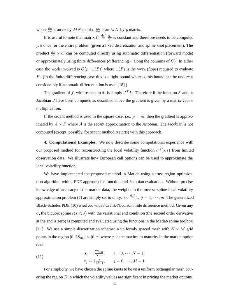
True Local Volatility

FIG. 2. The Reconstructed and True Local Volatility

optimization problem is relatively easy to solve. The optimization method requires 7 iterations

(6 Jacobian evaluations) and the computed optimal objective function value f(σ ∗) is 10−6.

Fig. 2 demonstrates the accuracy of this local volatility reconstruction: the reconstructed

spline surface c(s, t; σ∗) very accurately approximates the actual volatility surface σ ∗(s, t) in

the neighborhood of the region [75, 125]×[0, 1]. To better observe accuracy of reconstruction,

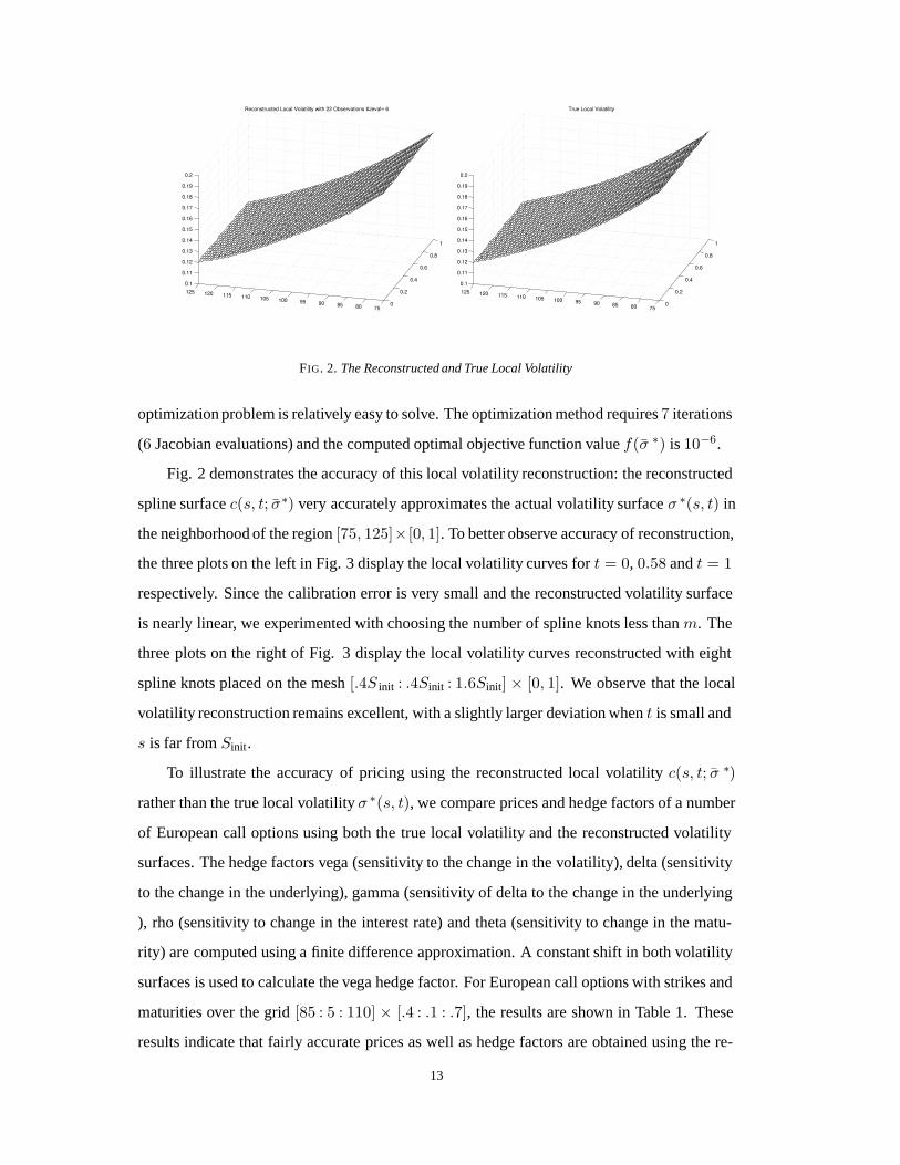
the three plots on the left in Fig. 3 display the local volatility curves for t = 0, 0.58 and t = 1

respectively. Since the calibration error is very small and the reconstructed volatility surface

is nearly linear, we experimented with choosing the number of spline knots less than m. The

three plots on the right of Fig. 3 display the local volatility curves reconstructed with eight

spline knots placed on the mesh [.4S init : .4Sinit : 1.6Sinit] × [0, 1]. We observe that the local

volatility reconstruction remains excellent, with a slightly larger deviation when t is small and

s is far from Sinit.

To illustrate the accuracy of pricing using the reconstructed local volatility c(s, t; σ ∗)

rather than the true local volatility σ ∗(s, t), we compare prices and hedge factors of a number

of European call options using both the true local volatility and the reconstructed volatility

surfaces. The hedge factors vega (sensitivity to the change in the volatility), delta (sensitivity

to the change in the underlying), gamma (sensitivity of delta to the change in the underlying

), rho (sensitivity to change in the interest rate) and theta (sensitivity to change in the matu-

rity) are computed using a finite difference approximation. A constant shift in both volatility

surfaces is used to calculate the vega hedge factor. For European call options with strikes and

maturities over the grid [85 : 5 : 110] × [.4 : .1 : .7], the results are shown in Table 1. These

results indicate that fairly accurate prices as well as hedge factors are obtained using the re-

13

75 80 85 90 95 100 105 110 115 120 1250.1

0.11

0.12

0.13

0.14

0.15

0.16

0.17

0.18

0.19

0.2Local Volatility Curves at t = 0.00

Index

Loca

l Vol

atili

ty

Exact Vol.Reconstructed Vol.

75 80 85 90 95 100 105 110 115 120 1250.1

0.11

0.12

0.13

0.14

0.15

0.16

0.17

0.18

0.19

0.2

Index

Loca

l Vol

atili

ty

Local Volatility Curves at t = 0.00


75 80 85 90 95 100 105 110 115 120 1250.1

0.11

0.12

0.13

0.14

0.15

0.16

0.17

0.18

0.19

0.2

Index

Loca

l Vol

atili

ty



75 80 85 90 95 100 105 110 115 120 1250.1

0.11

0.12

0.13

0.14

0.15

0.16

0.17

0.18

0.19


Loca

l Vol

atili

ty

Index


75 80 85 90 95 100 105 110 115 120 1250.1

0.11

0.12

0.13

0.14

0.15

0.16

0.17

0.18

0.19

0.2

Index

Loca

l Vol

atili

ty



75 80 85 90 95 100 105 110 115 120 1250.1

0.11

0.12

0.13

0.14

0.15

0.16

0.17

0.18

0.19


Index

Loca

l Vol

atili

ty


FIG. 3. Left: Knots = [0 : .2Sinit : 2Sinit] × [0, 1], Right: Knots = [.4Sinit : .4Sinit : 1.6Sinit] × [0, 1]

14

max relative error average relative error

Price 7.8e−3 2.1e−3

Vega 9.8e−3 6.1e−3

Delta 4.8e−2 1.3e−2

Gamma 9.5e−2 5.9e−2

Rho 4.5e−3 2.0e−3

Theta 6.9e−3 2.2e−3

TABLE 1

Accuracy of Pricing and Hedging

constructed volatility surface c(s, t; σ ∗). Note that the PDE option evaluation with the chosen

discretization can generate errors of at least these magnitudes.

We emphasize that the formulation (7) is appropriate when the number of spline knots p

is not greater than the number of observations m. If p is much larger than m, then formulation

(7) can become severely underdetermined. To illustrate the potential pitfalls of allowing too

much freedom in approximating σ∗(s, t), we simulate the more realistic market situation when

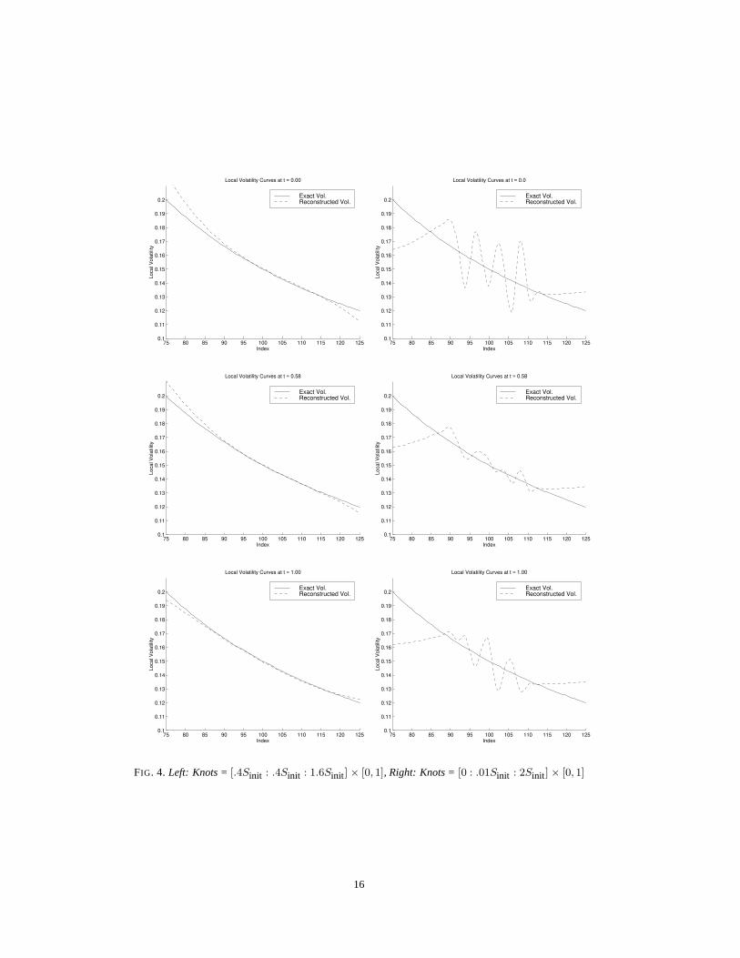
there is a bid-ask spread in the given option prices by setting

vj = exact price of option j + .02rand

where rand is a Matlab generated random number. We compare the local volatility reconstruc-

tions using the spline knots on the rectangular meshes [.4S init : .4Sinit : 1.6Sinit]× [0, 1] (p = 8)

and [0 : .01Sinit : 2Sinit]× [0, 1] (p = 202 < MN ). The plots on the left in Fig. 4 illustrate the

reconstructed local volatility curves using the rectangular mesh [.4S init : .4Sinit : 1.6Sinit]×[0, 1]

for knots. The plots on the right in Fig. 4 illustrate the reconstructed local volatility curves

using the rectangular mesh [0 :2 :2Sinit]× [0, 1] for knots. Although the available option prices

are matched with very high accuracy (error about 10−6) using p = 202, the computed local

volatility surface does not resemble the true local volatility surface σ ∗(s, t). Using eight knots

on the rectangular mesh [.4Sinit : .4Sinit : 1.6Sinit] × [0, 1], on the other hand, yields a much

more accurate volatility surface, even though the calibration error of the available options is

larger (about 10−4).

Next we illustrate that, assuming the underlying follows a continuous 1-factor model (1),

a constant implied volatility approach can produce erroneous hedge factors even though the

option prices may be computed accurately. We use the same absolute diffusion model (12)

but with greater volatility: the constant α = 75 is used instead of α = 15. The same initial

15

75 80 85 90 95 100 105 110 115 120 1250.1

0.11

0.12

0.13

0.14

0.15

0.16

0.17

0.18

0.19

0.2

Index

Loca

l Vol

atili

ty



75 80 85 90 95 100 105 110 115 120 1250.1

0.11

0.12

0.13

0.14

0.15

0.16

0.17

0.18

0.19

0.2

Index


Loca

l Vol

atili

ty


75 80 85 90 95 100 105 110 115 120 1250.1

0.11

0.12

0.13

0.14

0.15

0.16

0.17

0.18

0.19

0.2


Index

Loca

l Vol

atili

ty


75 80 85 90 95 100 105 110 115 120 1250.1

0.11

0.12

0.13

0.14

0.15

0.16

0.17

0.18

0.19

0.2


Index

Loca

l Vol

atili

ty


75 80 85 90 95 100 105 110 115 120 1250.1

0.11

0.12

0.13

0.14

0.15

0.16

0.17

0.18

0.19

0.2


Index

Loca

l Vol

atili

ty


75 80 85 90 95 100 105 110 115 120 1250.1

0.11

0.12

0.13

0.14

0.15

0.16

0.17

0.18

0.19

0.2

Index

Loca

l Vol

atili

ty



FIG. 4. Left: Knots = [.4Sinit : .4Sinit : 1.6Sinit] × [0, 1], Right: Knots = [0 : .01Sinit : 2Sinit] × [0, 1]

16

underlying Sinit = 100 and the risk free interest rate r = 0.05 are used but the dividend

rate q is set to zero. We consider European call options with strikes and maturities at the

grid [80 : 4 : 120] × [.25, .5, 1]. The spline knots are at the grid [0 : 20 : 2S init] × [0, .5, 1].

Fig. 5 displays the price and hedge factors of options with maturity .25 year using the true

local volatility, reconstructed volatility, and constant implied volatility. From these plots, we

see that the price and all the hedge factors computed using the reconstructed local volatility

function are fairly accurate approximation to the true values. Using the constant implied

volatility method, however, large errors exist in hedge factors (mostly noticeably in theta,

delta, gamma and vega).

In addition to choosing the number of spline knots p, the placement of the knots requires

some care as well. The spline knots should be placed to cover the region D within which

the values of the local volatility are significant in the option values. We have used the uni-

form spacing in the interval [0, 2S init] and [.4Sinit, 1.6Sinit] in this synthetic example but an

alternative is to place them nonuniformly with a more refined placement around s = S init.

Moreover, one need to avoid placing spline knots too closely together since this can lead to ill

conditioning of the Jacobian matrix ∇F .

4.2. A S&P 500 Example Illustrating Smoothness and Stability. We consider now a

more realistic example of approximating the local volatility function σ ∗(s, t) from the Euro-

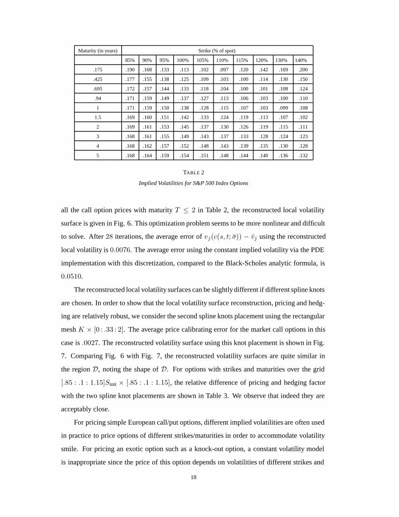
pean S&P 500 index European call options. We use the same European option data of October

1995 given in [1]. The market option price data (in the implied Black-Scholes constant volatil-

ity) is given in Table 2. Similar to [1], we use only the options with no more than two years

maturity in our computation. The initial index, interest rate and dividend rate are set as in [1],

Sinit = $590, r = 0.06, and q = 0.0262.

The discretization parameters in (11) are set as,

N = 101, and M = 101.

In order to solve the proposed inverse spline volatility problem (7), we compute the mar-

ket European call option prices with given strikes and maturities using the constant volatil-

ity Black-Scholes formula with the corresponding implied volatility. The Matlab function

blsprice is used.

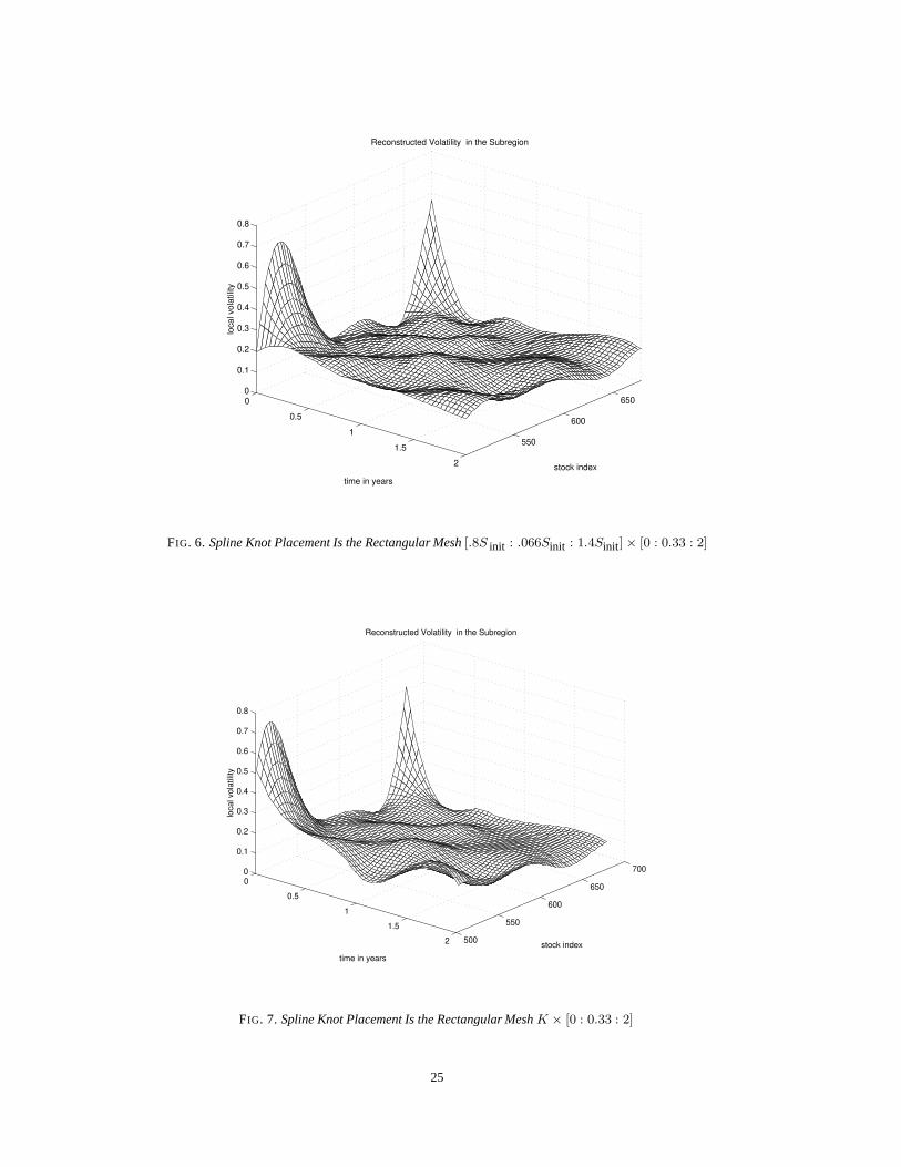
For this example the number of spline knots p equals the number of observations m and

the spline knots are placed on a rectangular mesh [.8S init : .066Sinit : 1.4Sinit]×[0 : .33:2].Using

17

Maturity (in years) Strike (% of spot)

85% 90% 95% 100% 105% 110% 115% 120% 130% 140%

.175 .190 .168 .133 .113 .102 .097 .120 .142 .169 .200

.425 .177 .155 .138 .125 .109 .103 .100 .114 .130 .150

.695 .172 .157 .144 .133 .118 .104 .100 .101 .108 .124

.94 .171 .159 .149 .137 .127 .113 .106 .103 .100 .110

1 .171 .159 .150 .138 .128 .115 .107 .103 .099 .108

1.5 .169 .160 .151 .142 .133 .124 .119 .113 .107 .102

2 .169 .161 .153 .145 .137 .130 .126 .119 .115 .111

3 .168 .161 .155 .149 .143 .137 .133 .128 .124 .123

4 .168 .162 .157 .152 .148 .143 .139 .135 .130 .128

5 .168 .164 .159 .154 .151 .148 .144 .140 .136 .132

TABLE 2

Implied Volatilities for S&P 500 Index Options

all the call option prices with maturity T ≤ 2 in Table 2, the reconstructed local volatility

surface is given in Fig. 6. This optimization problem seems to be more nonlinear and difficult

to solve. After 28 iterations, the average error of vj(c(s, t; σ)) − vj using the reconstructed

local volatility is 0.0076. The average error using the constant implied volatility via the PDE

implementation with this discretization, compared to the Black-Scholes analytic formula, is

0.0510.

The reconstructed local volatility surfaces can be slightly different if different spline knots

are chosen. In order to show that the local volatility surface reconstruction, pricing and hedg-

ing are relatively robust, we consider the second spline knots placement using the rectangular

mesh K × [0 : .33 : 2]. The average price calibrating error for the market call options in this

case is .0027. The reconstructed volatility surface using this knot placement is shown in Fig.

7. Comparing Fig. 6 with Fig. 7, the reconstructed volatility surfaces are quite similar in

the region D, noting the shape of D. For options with strikes and maturities over the grid

[.85 : .1 : 1.15]Sinit × [.85 : .1 : 1.15], the relative difference of pricing and hedging factor

with the two spline knot placements are shown in Table 3. We observe that indeed they are

acceptably close.

For pricing simple European call/put options, different implied volatilities are often used

in practice to price options of different strikes/maturities in order to accommodate volatility

smile. For pricing an exotic option such as a knock-out option, a constant volatility model

is inappropriate since the price of this option depends on volatilities of different strikes and

18

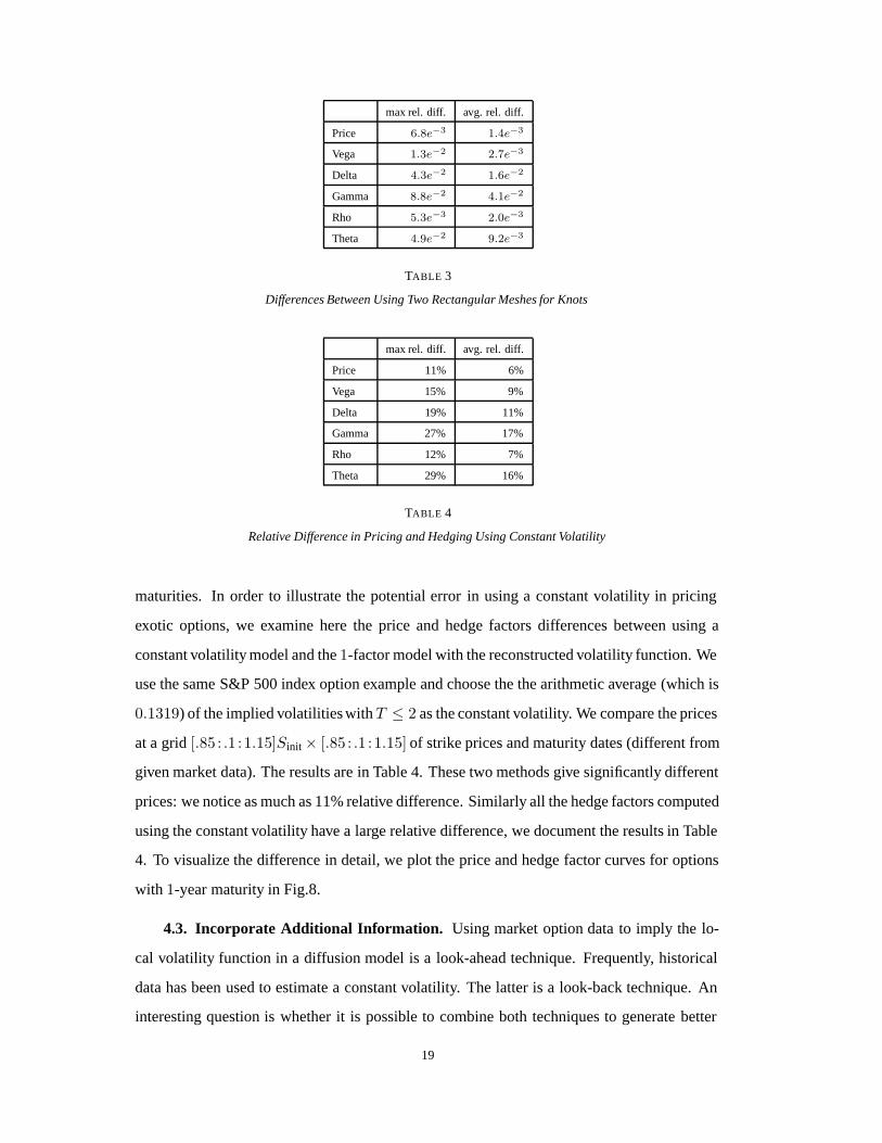
max rel. diff. avg. rel. diff.

Price 6.8e−3 1.4e−3

Vega 1.3e−2 2.7e−3

Delta 4.3e−2 1.6e−2

Gamma 8.8e−2 4.1e−2

Rho 5.3e−3 2.0e−3

Theta 4.9e−2 9.2e−3

TABLE 3

Differences Between Using Two Rectangular Meshes for Knots

max rel. diff. avg. rel. diff.

Price 11% 6%

Vega 15% 9%

Delta 19% 11%

Gamma 27% 17%

Rho 12% 7%

Theta 29% 16%

TABLE 4

Relative Difference in Pricing and Hedging Using Constant Volatility

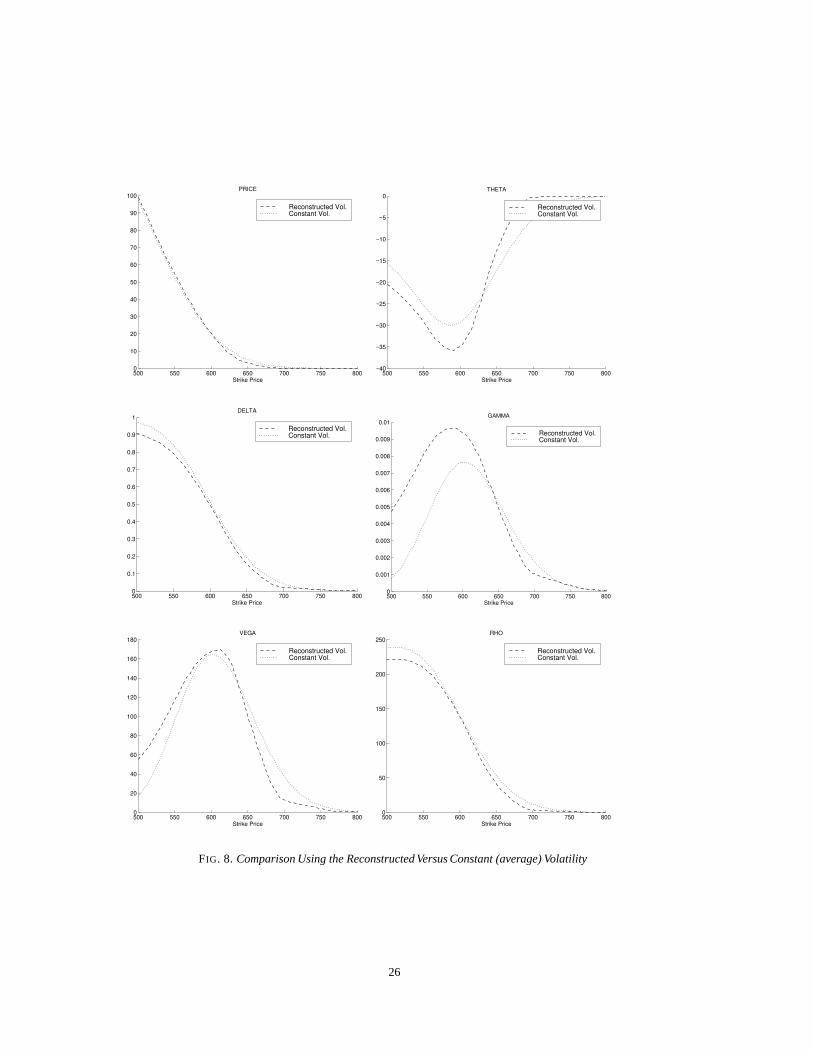
maturities. In order to illustrate the potential error in using a constant volatility in pricing

exotic options, we examine here the price and hedge factors differences between using a

constant volatility model and the 1-factor model with the reconstructed volatility function. We

use the same S&P 500 index option example and choose the the arithmetic average (which is

0.1319) of the implied volatilities with T ≤ 2 as the constant volatility. We compare the prices

at a grid [.85: .1 :1.15]Sinit × [.85: .1 :1.15] of strike prices and maturity dates (different from

given market data). The results are in Table 4. These two methods give significantly different

prices: we notice as much as 11% relative difference. Similarly all the hedge factors computed

using the constant volatility have a large relative difference, we document the results in Table

4. To visualize the difference in detail, we plot the price and hedge factor curves for options

with 1-year maturity in Fig.8.

4.3. Incorporate Additional Information. Using market option data to imply the lo-

cal volatility function in a diffusion model is a look-ahead technique. Frequently, historical

data has been used to estimate a constant volatility. The latter is a look-back technique. An

interesting question is whether it is possible to combine both techniques to generate better

19

Tol Finite Difference quasi-Newton Update

Iterations Time Iterations Time J evals

1e−2 7 321.29 11 131.85 3

1e−3 10 401.43 18 193.91 4

1e−4 19 651.89 28 286.78 5

1e−5 25 795.45 36 332.13 6

TABLE 5

Quasi Newton Results

approximation to the local volatility function.

In the proposed spline volatility formulation (7), there are two potential ways that a priori

information can be incorporated. The first is to use the simple bounds to limit the range of the

local volatilities at knots. The second possibility is to specify fixed local volatilities at some

chosen knots.

We have experimented with setting tighter bounds on the volatility σ for the S&P 500

index European call option example. We observe that, as long as the bounds are not too small

(l ≤ −.3, , u ≥ .3 in the S&P 500 example), they can influence volatility values of small t

and s far from Sinit but do not have much impact in the region D within which the volatility

function is significant in market option prices. However, setting bounds too tight can impede

calibrating the market option prices. Therefore, unless one has reliable knowledge on the

bounds of the volatilities, they should be sufficiently large to ensure that the calibrating error

is sufficiently small. Similar remarks can be made if one wishes to set the volatilities at certain

knots to some fixed values.

Finally, we would like to illustrate the potential computational saving by using the quasi-

Newton updates. In Table 5 we present Matlab computational results using the finite dif-

ference and quasi-Newton update for Jacibian for the S&P 500 index option example with

different termination tolerances for optimization. We observe significant total speedup using

a quasi-Newton approach. The quasi-Newton approach takes more iterations to converge but

requires fewer Jacobian evaluations.

5. Concluding Remarks. Assuming that the underlying asset of options follows a con-

tinuous 1-factor diffusion model, we propose a method of accurately approximating the local

volatility function σ ∗(s, t) using a finite set of option prices. We emphasize that accurate

approximation of the local volatility function in the 1-factor model is crucial in hedging all

20

options (including simple European options) and pricing exotic options. Moreover, since the

market option data typically has bid-ask spreads, exact calibration of the option data (the

average of the bid-ask spreads) is not necessary and can be harmful.

Based on the formula (6) established in [1, 17], the local volatility function σ ∗(K, T )2

is smooth if the European call option value function v(K, T ) is sufficiently smooth. We use

a spline functional approach to reconstruct this local volatility function. After choosing the

number of spline knots and their placement, we represent a local volatility function σ(s, t) by

an interpolating spline with a fixed end condition. The volatility values at knots are determined

by solving a small nonlinear optimization problem subject to simple bounds. The number of

variables in the optimization (7) is no greater than the number of option observations.

We solve the proposed inverse spline approximation optimization problem using a trust

region method, with the function and Jacobian evaluated using a PDE approach. Computa-

tional efficiency through structure exploitation within the framework of finite difference and

automatic differentiation is discussed.

We consider two European call options examples illustrating the capability of the pro-

posed method. In the first example, we consider synthetic European call options for which the

underlying follows a known absolute diffusion model. Option observation data is simulated

by evaluating a set of European call options using the analytic formula. The reconstructed

local volatility is compared to the true local volatility, indicating a fairly accurate reconstruc-

tion in the region within which the local volatility values are significant for option evaluations.

With the same example, we illustrate that the constant implied volatility approach can produce

erroneous hedge factors, compared to that from the 1-factor model, even for simple European

options. Moreover, when the observable option prices have bid-ask spreads, calibrating mar-

ket data exactly by using too many spline knots can lead to poor reconstruction of the true local

volatility function. In the second example, S&P 500 index European call options with market

option data of October 1995 are considered. We illustrate the smoothness of the reconstructed

local volatility and stability of the proposed method in pricing and hedging.

We have demonstrated the potential of the proposed spline volatility approach in discov-

ering, from a finite set of option prices, the local volatility function in the 1-factor process fol-

lowed by the underlying. We plan to further investigate automatic techniques for the optimal

selection of the number of knots p ≤ m and their placement. The importance of the proposed

local volatility function reconstruction in pricing exotic options or American options will also

21

be explored.

6. Acknowledgement. We would like to thank Yohan Kim for carefully reading the

manuscript and his useful comments. We also thank Bob Jarrow for his encouragement.

REFERENCES

[1] L. ANDERSEN AND R. BROTHERTON-RATCLIFFE, The equity option volatility smile: an implicit finite-

difference approach, The Journal of Computational Finance, 1 (1998), pp. 5–32.

[2] M. AVELLANEDA, C. FRIEDMAN, R. HOLEMES, AND D. SAMPERI, Calibrating volatility surfaces via

relative entropy minimization, Applied Mathematical Finance, 4 (1997), pp. 37–64.

[3] G. BIRKHOFF AND C. R. DE BOOR, Piecewise polynomial interpolation and approximation, in Approxi-

mation of Functions, H. L. Garabedian, ed., Elsevier (New York), 1965, pp. 164–190.

[4] F. BLACK AND M. SCHOLES, The pricing of options and corporate liabilities, Journal of Political Econ-

omy, 81 (1973), pp. 637–659.

[5] I. BOUCHOUEV AND V. ISAKOV, The inverse problem of option pricing, Inverse Problems, 13 (1997),

pp. L11–L17.

[6] M. A. BRANCH, T. F. COLEMAN, AND Y. LI, A subspace, interior and conjugate gradient method for

large-scalebound-constrainedminimization, Tech. Report TR95-1525, Computer Science Department,

Cornell University, 1995.

[7] T. F. COLEMAN AND Y. LI, An interior, trust region approach for nonlinear minimization subject to

bounds, SIAM Journal on Optimization, 6 (1996), pp. 418–445.

[8] T. F. COLEMAN AND A. VERMA, Structure and efficient Jacobian calculation, in Computational Differen-

tiation: Techniques, Applications, and Tools, M. Berz, C. Bischof, G. Corliss, and A. Griewank, eds.,

SIAM, Philadelphia, Penn., 1996, pp. 149–159.

[9] J. C. COX AND S. A. ROSS, The valuation of options for alternative stochastic processes, Journal of

Financial Economics, 3 (1976), pp. 145–166.

[10] S. R. DAS AND R. K. SUNDARAM, Of smiles and smirks: A term-structure perspective, Tech. Report

NBER working paper No. 5976, Department of Finace, Harvard Business School, Harvard University,

Boston, MA 02163, 1997.

[11] C. DE BOOR, Spline Toolbox for use with MATLAB, The Math Works Inc., 1997.

[12] J. E. DENNIS AND R. B. SCHNABEL, Numerical Methods for Unconstrained Optimization, Prentice-Hall,

1983.

[13] E. DERMAN AND I. KANI, Riding on a smile, Risk, 7 (1994), pp. 32–39.

[14] , The local volatility surface: Unlocking the information in index option prices, Financial Analysts

Journal, (1996), pp. 25–36.

[15] P. DIERCKX, An algorithm forsurface fitting with spline functions, IMA Journal of Numerical Analysis, 1

(1981), pp. 267–283.

[16] , Curve and Surface Fitting with Splines, Oxford Science Publications, 1993.

[17] B. DUPIRE, Pricing with a smile, Risk, 7 (1994), pp. 18–20.

22

[18] A. GRIEWANK, Some bounds on the complexity of gradients, Jacobians, and Hessians, in Complexity in

Nonlinear Optimization, P. Pardalos, ed., World Scientific Publishers, 1993, pp. 128–161.

[19] D. HEATH, R. JARROW, AND A. MORTON, Bond pricing and the term structure of interest rates: A new

methodology for contingent claims valuation, Econometrica, 60 (1992), pp. 77–105.

[20] J. HULL AND A. WHITE, The pricing of options on assets with stochastic volatilities, Journal of Finance,

3 (1987), pp. 281–300.

[21] N. JACKSON, E. SULI, AND S. HOWISON, Computation of deterministic volatility surfaces, Tech. Report

No. 98/01, Oxford University Computing Laboratory, 1998.

[22] J. JACKWERTH AND M. RUBINSTEIN, Recoveringprobability distributions from option prices, The Journal

of Finance, 51 (1996), pp. 1611–1631.

[23] R. LAGNADO AND S. OSHER, Reconciling differences, Risk, 10 (1997), pp. 79–83.

[24] D. LAMBERTON AND B. LAPEYRE, Introduction to Stochastic Calculus Applied to Finance, Chapman &

Hall, 1996.

[25] R. MERTON, The theory of rational option pricing, Bell Journal of Economics and Management Science,

4 (1973), pp. 141–183.

[26] , Option pricing when underlying stock returns are discontinuous, Journal of Financial Economics, 3

(1976), pp. 124–144.

[27] M. RUBINSTEIN, Implied binomial trees, The Journal of Finance, 49 (1994), pp. 771–818.

[28] D. SHIMKO, Bounds of probability, Risk, (1993), pp. 33–37.

[29] A. N. TIKHONOV AND V. Y. ARSENIN, Solutions of Ill-posed Problems, W. H. Winston, Washington,

D.C., 1977.

[30] V. N. VAPNIK, Estimation of Dependences Based on Empirical Data, Springer-Verlag, Berlin, 1982.

[31] G. WAHBA, Splines Models for Observational Data, Series in Applied Mathematics, Vol. 56, SIAM,

Philadelphia, 1990.

[32] R. ZVAN, K. VETZAL, AND P. FORSYTH, Swing high Swing low, Risk Magazine, (1998), pp. 71–74.

23

80 90 100 110 120 130 140 1500

5

10

15

20

25

30

Strike Price

PRICE

True Vol.Reconstructed Vol.Implied Vol.

80 90 100 110 120 130 140 150−23

−22

−21

−20

−19

−18

−17

−16

−15

−14

80 90 100 110 120 130 140 150−23

−22

−21

−20

−19

−18

−17

−16

−15

−14

Strike Price

THETA


80 90 100 110 120 130 140 1500.1

0.2

0.3

0.4

0.5

0.6

0.7

0.8

Strike Price

DELTA


80 90 100 110 120 130 140 1504

5

6

7

8

9

10

11

12x 10

−3

Strike Price

GAMMA


80 90 100 110 120 130 140 1508

10

12

14

16

18

20

22

Strike Price

VEGA


80 90 100 110 120 130 140 1502

4

6

8

10

12

14

Strike Price

RHO


FIG. 5. Comparison Between Using the True, Reconstructed and Constant Implied Volatility Functions

24

0

0.5

1

1.5

2

550

600

6500

0.1

0.2

0.3

0.4

0.5

0.6

0.7

0.8

stock index

Reconstructed Volatility in the Subregion

time in years

loca

l vol

atili

ty

FIG. 6. Spline Knot Placement Is the Rectangular Mesh [.8S init : .066Sinit : 1.4Sinit] × [0 : 0.33 : 2]

0

0.5

1

1.5

2 500

550

600

650

7000

0.1

0.2

0.3

0.4

0.5

0.6

0.7

0.8

stock index

Reconstructed Volatility in the Subregion

time in years

loca

l vol

atili

ty

FIG. 7. Spline Knot Placement Is the Rectangular Mesh K × [0 : 0.33 : 2]

25

500 550 600 650 700 750 8000

10

20

30

40

50

60

70

80

90

100

Strike Price

PRICE

Reconstructed Vol.Constant Vol.

500 550 600 650 700 750 800−40

−35

−30

−25

−20

−15

−10

−5

0

Strike Price

THETA


500 550 600 650 700 750 8000

0.1

0.2

0.3

0.4

0.5

0.6

0.7

0.8

0.9

1

Strike Price

DELTA


500 550 600 650 700 750 8000

0.001

0.002

0.003

0.004

0.005

0.006

0.007

0.008

0.009

0.01

Strike Price

GAMMA


500 550 600 650 700 750 8000

20

40

60

80

100

120

140

160

180

Strike Price

VEGA


500 550 600 650 700 750 8000

50

100

150

200

250

Strike Price

RHO


FIG. 8. Comparison Using the Reconstructed Versus Constant (average) Volatility

26

reconstructing the unknown local volatility …janroman.dhis.org/finance/volatility models/local...

Documents