View-Dependent Multiscale Fluid Simulation

Yue Gao 1, Chen-Feng Li 2, Bo Ren 1 and Shi-Min Hu 1

Technical Report TR-110830

Tsinghua University, Beijing, China

1 Department of Computer Science and Technology, Tsinghua University

2 College of Engineering, Swansea University

TECHNICAL REPORT 110830 1

View-Dependent Multiscale Fluid SimulationYue Gao, Chen-Feng Li, Bo Ren, and Shi-Min Hu

Abstract—Fluid motions are highly nonlinear and non-stationary, with turbulence occurring and developing at different length and timescales. In real-life observations, the multiscale flow generates different visual impacts depending on the distance to the viewer. Wepropose a new fluid simulation framework that adaptively allocates computational resources according to the human visual perception.First, a 3D empirical model decomposition scheme is developed to obtain the velocity spectrum of the turbulent flow. Then, dependingon the distance to the viewer, the fluid domain is divided into a sequence of nested simulation partitions. Finally, the multiscale fluidmotions revealed in the velocity spectrum are distributed non-uniformly to these view-dependent partitions, and the mixed velocityfields defined on different partitions are solved separately using different grid sizes and time steps. The fluid flow is solved at differentspatial-temporal resolutions, such that higher-frequency motions closer to the viewer are solved at higher resolutions and vice versa.The new simulator better utilizes the computing power, producing visually plausible results with realistic fine-scale details in a moreefficient way. It is particularly suitable for large scenes with the viewer inside the fluid domain. Also, as high-frequency fluid motions aredistinguished from low-frequency motions in the simulation, the numerical dissipation is effectively reduced.

Index Terms—fluid simulation, Hilbert-Huang transform, fluid velocity spectrum, view-dependent partition.

F

1 INTRODUCTION

Fluid simulations based on the Navier-Stokes equationshave achieved great success in computer graphics. Manycompelling methods with impressive animations havebeen reported in the past decade. However, fluid simu-lation remains a challenging task where improving thevisual effect of fine-scale fluid motions and reducingthe demand of computational resources are the mainconcerns. Unlike computational physics, the focus ofgraphics applications is on the visual effect of the finalrendered images and animations. This implies a highpotential value for exploiting the unique viewing in-formation to improve existing fluid simulators. In thiswork, we propose a novel approach which incorporatesthe viewing information into the fluid solver and adap-tively simulates the fluid at multiple scales, such that thecomputational resources are allocated to the key regionsand to the key scales that have important impacts onthe visual impression of turbulent fluids. This approachis particularly suitable for large scenes with the viewerimmersed in the fluid domain. Such kind of scenes arerare to be seen in previous publications, but are oftenmost desired by movie directors and game designers.

Generally, the techniques considering the viewer arereferred as the levels of details, which has become astandard tool widely used in 3D geometry representationand texture rendering. The basic idea is that whenthe object is far from the viewer, a reduced geometryrepresentation or a reduced texture is applied. Thissimplification is supported by the fact that, for humanvisual perception, the higher frequency signals play a

• Y. Gao, B. Ren and S.M. Hu are with the Department of Computer Science,Tsinghua University, Beijing 100084, China.

• C.F. Li is with the College of Engineering, Swansea University, SwanseaSA2 8PP, UK.

more important role when the viewer is nearby, whilethe lower frequency signals are more important whenthe viewer is at distance [1].

Inspired by view-dependent rendering techniques, wefirst decompose the fluid velocity field into a series offrequency components using a modified empirical modedecomposition (EMD) method. Higher frequency com-ponents represent smaller scale fluid motions (typicallylocal turbulent flow), while lower frequency componentsrepresent motions at larger scales (typically large eddiesand global laminar flow). Also, the fluid domain isdivided into a series of nested partitions centered withrespect to the viewing frustum. Different grid sizes andtime steps are assigned to different partitions dependingon their distances to the viewer. The control of levelsof details is then applied to each frequency compo-nent by distributing it non-uniformly to the simulationpartitions. Higher frequency components closer to theviewer are allocated to partitions with finer grids andsmaller time steps, while lower frequency componentsmore far away from the viewer are allocated to partitionswith coarser grids and larger time steps. As a result,the effective velocity field defined on each simulationpartition is a mixture of frequency components, and thevisible evolution of the mixed velocity can be sufficientlycaptured by the space-time resolution associated withthe specific partition. To obtain the final solution, theeffective velocity fields are solved semi-independentlyon different partitions, which provides richer visual de-tails to the viewer in a more efficient way. Although thenested simulation partitions differ in size and resolution,they are all meshed with uniform rectangular grids,which makes the solver robust and efficient.

This novel view-dependent multiscale simulationframework distributes the computational resources ac-cording to the human visual perception of the targetfluid motion, and is adaptive in both space and time

TECHNICAL REPORT 110830 2

Fig. 1. Four snapshots of a view-dependent multiscale fluid simulation with moving camera positions. (6 partitions,grid sizes: 1/400 – 1/100, time steps: 1/120 s – 1/30 s)

dimensions. The main technical innovations include:• Using a novel approach of space-filling curves, the

EMD is efficiently extended to 3D and applied todecompose the velocity field into a small numberof frequency components, which represent the fluidmotion at different length scales.

• A spectrum based simulation pipeline is proposed,in which different frequency components evolveat different space-time resolutions. By doing so, itsignificantly reduces the numerical diffusion thatcauses damping of high frequency turbulence inprevious methods, and preserves more fine-scaleturbulence details in the result.

• The fluid domain is adaptively partitioned accord-ing to the camera position, and the fluid is simulatedat different space-time resolution depending on itsdistance to the viewer. This approach considers bothrendering and simulation together, and efficientlyutilizes the computational resources in the placesthat most affect the final rendered result.

2 PREVIOUS WORKS

Jos Stam’s unconditionally stable solver [2] made thegrid-based fluid simulation popular in the graphicscommunity. Since then, many different techniques havebeen developed to add details to the fluid. The basicapproach is to reduce the numerical dissipation (alsoknown as “numerical diffusion”). [3] used the vorticityconfinement technique to prevent the rapid dissipationof vortices. [4] introduced artificial divergence sources tosimulate gas explosion. [5] introduced vortex particlesto add the vorticity more accurately. [6] introducedFLIP to overcome advection dissipation. Other methodsincluding BFECC [7], QUICK [8], MacCormack [9] sug-gested using higher-order space discretization schemesand higher-order time integration schemes (e.g. Runge-Kutta methods). These methods discretize the wholefluid domain using uniform grids, thus they are alllimited by the Nyquist frequency.

For 3D fluid simulation, a small increase of the gridresolution by a factor of k will cause a dramatic increaseto the computational cost by a factor of k4 [10]. There-fore, various techniques have been investigated in order

to increase the simulation resolution while controllingthe computational expense. [11], [12], [13], [14] proposeddifferent methods to generate divergence free fields fromrandom noise, and then used these artificial velocityfields to represent the turbulent flow. [15], [16], [17],[18], [19] simulated the fluid on a low-resolution gridto obtain the macro-scale flow, which was then com-bined with the artificial divergence-free velocity fieldsto mimic the turbulent flow at the micro scale. Insteadof adding noise, [20] used the vortex particle method[5] to directly generate a high-resolution turbulent flow,and [13] synthesized the 3D velocity field from 2Dslices. These synthesis methods do not perform high-resolution computation on the Navier-Stokes equations,and instead attempt to produce plausible results usingartificial means. Thus, their results are nonphysical, butcan be combined with any grid-based method.

Although grid-based fluid solvers are often preferredin the graphics community, other numerical schemes in-cluding finite volume [21], [22] and finite element meth-ods [23] have also been used in many specific graphicsapplications. Some researchers have also exploited theviewing information in fluid simulations. Until recently,there have been mainly two types of approaches: (a)octree and adaptive mesh refinement methods [24], [25],which use non-uniform meshes to distinguish differentlevels of details for the fluids; and (b) multi-grid methods[8], [10], [26], which use multiple layers of meshes torepresent fluid motions at different length scales. Theidea of multi-grid simulations has also been adoptedin the framework of smoothed-particle hydrodynamicsto accelerate fluid simulation [27]. In a wider context,it is also noted that [28] presented a view-dependentmultiscale simulation framework for fire simulations.

3 ALGORITHM OVERVIEW

Fluid phenomena are interesting and visually attractivebecause of turbulent fluid motions. It is well knownin fluid dynamics that turbulence occurs and developsat different length and time scales, with the extent ofscale difference indicated by the Reynolds number. Inorder to capture fine-scale features of turbulent flows,it is normally necessary to use fine simulation grids

TECHNICAL REPORT 110830 3

Velocity

Field +

+

=

N-S

Solver

N-S

Solver

N-S

Solver

+

+

=

...

...

...

Ω1

Ω2

Ωm

*

1u

*

2u

*

mu

1u

2u

mu

Fig. 2. The algorithm framework of view-dependent multiscale fluid simulation

and small time steps, or to use higher-order space dis-cretization and time integration schemes. This creates ahuge computational burden to the fluid simulator, inparticular when simulating a large fluid domain. Onthe other hand, objects in a large scene are observed atdifferent resolutions by human eyes depending on theirdistances to the viewer. Fine local fluid motions havea significant visual impact when the viewer is nearby,and as the distance to the viewer increases, these fine-scale features become less and less visible, while globalfluid motions at larger scales becoming more and moredominant. Thus, for the purpose of achieving visuallyappealing results, there is a clear potential of benefitof utilizing the viewing information to improve theperformance of fluid simulators.

We propose a view-dependent multiscale simulationframework as shown in Fig. 2. First, the fluid velocityfield is decomposed into a series of frequency com-ponents u1, u2, · · ·, um, representing the fluid motionat different length scales ranging from small to large.Next, according to the position of the viewer, m nestedsimulation partitions Ωi are constructed, with Ω1 indicat-ing the vicinity of the viewer and Ωm representing thewhole fluid domain. These simulation partitions are allmeshed into uniform rectangular grids, and each parti-tion Ωi is set with a different grid size depending on thelength scale of the corresponding frequency componentui. Then, each frequency component ui is sequentiallyallocated to partitions Ωi, Ωi+1, · · ·, Ωm, such that foreach partition, it only carries the component quantitythat has not been supported by the previous ones. Thus,the effective velocity field u∗i defined on partition Ωi

is a mixture of velocity components u1, · · ·, ui thatshare a similar visual significance determined by theirintrinsic length scales and distances to the viewer. Tosolve this combined velocity field u∗i with uniform visualsignificance, a separate fluid simulation is performed onpartition Ωi with individually assigned grid size and

time step. Finally, the total fluid motion in the wholefluid domain is constructed by adding up the resultsobtained on all simulation partitions. Depending on thefluid evolution, the velocity spectrum is repeatedly com-puted to ensure that the new fluid motion is efficientlyrepresented by the frequency components u1, · · ·, um.

The proposed view-dependent multiscale fluid simu-lation framework can be viewed as a multi-grid methodcombined with spectral decomposition. The idea of us-ing spectral analysis in CFD applications is not entirelynew, and a remarkable example is the large eddy sim-ulation [29] that introduces spatial-temporal filters toreduce the range of length scales of the solution, hencereducing the computational cost. The feasibility of thisnew simulation framework relies on two assumptions:(a) the fluid velocity field can be decomposed into asmall number of meaningful frequency components atdifferent length scales; and (b) the Navier-Stokes equa-tions can be linearized to allow separately solving eachfrequency component with varying grids and varyingtime steps. The consideration and solution of these twoissues are addressed in Sections 4 and 5 respectively.

4 3D VELOCITY FIELD DECOMPOSITION

The fluid velocity field can be viewed as a time-varyingsignal defined in a 3D domain. From the viewpoint ofphysics, it is clear that the 3D velocity signal consists ofintrinsic structures at different length scales. However,as turbulence is highly nonlinear and non-stationary,standard data analysis tools such as singular valuedecomposition [30], Fourier and wavelet analysis etc.typically produce many spurious frequency componentscausing energy spreading, which makes the resultingspectrum have little physical meaning. An exceptionis the empirical mode decomposition (EMD) [31], alsoknown as Hilber-Huang transform, which was originallydeveloped for processing nonlinear and non-stationary

TECHNICAL REPORT 110830 4

time series. Over the past decade, the EMD method hasbeen extremely successful in engineering and success-fully applied in various complicated data sets, includingsea waves and earthquake signals etc.

For the sake of completeness, the standard EMD pro-cedure is briefly reviewed in Section 4.1, after which itis extended into 3D cases in Section 4.2 for processingthe fluid velocity field.

4.1 EMD BasicsThe standard EMD method is designed for the analysisof one-dimensional signals, in particular time series. Themain idea of EMD is to decompose the signal into asmall number of intrinsic mode functions (IMF), whichare based on and derived from the data. An IMF isany function with the same number of extrema andzero crossings, and with zero mean of the upper andlower envelops defined respectively by the local maximaand minima. From this definition, the IMF is a generaloscillatory function, with possibly varying amplitudeand frequency along the time axis. Thus, for representingsignals, an IMF is much more powerful than the simpleharmonic function, which has constant amplitude andfrequency. Given a one-dimensional signal f , the EMDalgorithm sequentially extracts its IMFs via a “sifting”procedure as follows:

1) Initialization r0 = f , set index k = 12) Compute the k-th IMF, ck

a) Initialization h0 = rk−1, set index j = 1b) Find all local maxima and local minima of

hj−1

c) Build the upper envelope Emax,j−1 by con-necting all local maxima with a cubic spline,and build the lower envelope Emin,j−1 byconnecting all local minima with a cubic spline

d) Compute the mean of the upper and lower en-velopes, Emean,j−1 = 1

2 (Emin,j−1 + Emax,j−1)e) hj = hj−1 − Emean,j−1

f) If the IMF stopping criterion is satisfied, thenck = hj , else j = j + 1 and go to step 2(b)

3) rk = rk−1 − ck4) If rk is monotonic, the decomposition stops, else

k = k + 1 and go to step 2The signal f is decomposed as

f =K∑

k=1

ck + rK , (1)

where ci, i = 1, 2, ..,K are the IMFs with the frequencyranging from high to low, and rK is the residual.

For the IMF stopping criterion in step 2(f), differentcriteria have been suggested in the literature based onthe definition of IMFs. In our applications, it is foundthat there is no visible difference in the final result ifwe simply fix the iteration number as 8 to 10. There isno rigorous convergence proof for the above algorithm,but practically it always converges very quickly [31]. The

physical justification of the above EMD procedure is verysolid and has been verified and validated in numerousexperiments by various real data sets (see e.g. [32]).

4.2 3D EMD of Velocity Fields

The main challenge of extending the EMD into higher di-mensional signals arises in the construction of the upperand lower envelopes (step 2(c) in the EMD algorithm).Unlike the simple closed-form solution of the 1D cubicspline interpolation, higher dimensional surface inter-polation is complex and often involves time-consumingcomputation. For the 2D case, [33] and [34] introduced2D radial basis functions and transformed the interpo-lation problem into a global optimization problem. Itrequires to solve a m×m linear system, where m is thetotal number of extrema. The associated computation isaffordable for 2D image applications with hundreds ofpixels along each axis, but is too slow for our 3D fluidsimulations that require the EMD to be repeatedly per-formed in a large 3D space as turbulence develops. [35]proposed a fast bidimentional EMD algorithm, which isbased on the Delaunay triangulation and cubic inter-polation on triangles. In order to ensure the Delaunaytriangulation to cover the whole domain, this methodhas to introduce a bunch of artificial extrema, and as aresult it is not suitable for our 3D fluid simulations thatrequire the highest level of automation and robustness.[36] tested a tensor-product based 2D EMD approachthat applies separately 1D EMD on each row and columnof an image, after which averaging the envelopes fromdifferent directions. Although it is much faster to do so,our experiments led to a similar conclusion as [36]: theresult is generally worse in that each slice of data onlycontain a small portion of samples and the connectioninformation contained in the original data has beenseriously lost. As the EMD will be repeatedly performedin our fluid simulation framework, a more efficient andmore robust 3D algorithm is needed.

We propose to use space-filling curves to flatten 3Ddata into 1D. First, a space filling curve is constructedto fill the fluid domain, and moving along the curvean index is assigned to each grid cell and saved in atemplate. Then, the 3D velocity field is rearranged into a1D signal array according to the index template. Finally,the reshaped 1D signal is decomposed by using the 1DEMD algorithm, and the decomposition result is mappedback to the 3D space by using the same index template.In this simple 3D EMD approach, the EMD operation isessentially performed on the flattened 1D data set, andtherefore it converges in the same way as the standard1D EMD method [31]. As the index template of space-filling curve can be pre-computed, the CPU expense ofthe 3D EMD is essentially the same as 1D EMD, whichis linearly proportional to the sampling density. Owingto the analytic cubic spline interpolation, our space-filling curve EMD technique is extremely fast. For 2Dcases, we have compared with the RBF method. It is

TECHNICAL REPORT 110830 5

(a) (b) (c) (d)

Fig. 3. Decomposition comparison of a 2D fluid velocity field. The top row shows Fourier decomposition, and thebottom row shows the EMD result. (a)-(d) are the 1st, 3rd, 4th, and 5th components from low frequency to highfrequency. The EMD and Fourier results are obtained with the same sampling resolution.

found that our approach is at least 20 times faster in alltest examples, and the new method also provides betteraccuracy because it avoids the numerical error causedby the least squares approximation required in the RBFapproach. In the context of fluid simulation, the CPUcost of an individual 3D EMD is about half of a singlepressure solver executed on the same sampling grid.

Different space-filling curves have been tested, includ-ing the Hilbert curve, the Z-order curve, the Koch curveand the Gosper curve. In 2D cases, the Hilbert curve andthe Z-order curve are found to have boundary artifactscaused by their regular quad fractal structures. By usingKoch or Gosper curves, the boundary artifacts can beeffectively removed. In 3D cases, all four curves givegood decomposition results without visible discontinu-ities. The reason is that both the 3D velocity filed and the3D space filling curves are sufficiently complex to avoidthe development of boundary artifacts. For the sakeof simplicity, we use the Koch curve for 2D examplesand the Hilbert curve for 3D examples in this paper.It is noted that the Z-order curve has recently been inSPH simulations to compute SPH neighborhoods rapidly[37], which also demonstrates the benefit of using space-filling curves to accelerate 3D data processing.

The 3D Hilbert curve is defined on a cube, and whenusing the n-th approximation to the limiting curve, thelength of the curve is 2n. However, the fluid domain isnot necessarily a cube. Therefore, we build the Hilbertcurve with the smallest n such that 2n/3 is greaterthan the maximum velocity resolution in x-, y- and z-directions. When moving along the Hilbert curve, the cellindex is increased and saved if and only if the current

Fig. 4. Quadric KochCurve.

1 2 3 4 50

5

10

15

20

25

30

35

40

45

50

ComponentE

nerg

y/To

tal E

nerg

y(%

)

EMD DecompositionFourier Decomposition

Fig. 5. Energy distribu-tion of the lowest 5 fre-quency components.

(a) (b) (c)

Fig. 6. Reconstruction comparison. (a) is the originalvelocity field, (b) is the sum of the first 5 EMD componentsand (c) is the sum of the first 5 Fourier components.

position is located in the fluid domain. A similar methodis applied to the Koch curve in 2D cases. In Fig. 4, thegray line is the whole Koch curve and the bold black lineis the space filling curve we used. This strategy preservesas much as possible the locality of the space filling curve.

To flatten 3D data into 1D for EMD operations is an

TECHNICAL REPORT 110830 6

approximate treatment, and so doing inevitably causessome loss of local connectivity information presented inthe original 3D data. For use in fluid simulation, wehave tested the new space-fill curve EMD approach innumerous examples, both in 2D and 3D. Fig. 3 is an2D example of our EMD result compared with Fourierdecomposition. The velocity field is generated by usinga 2D grid solver and for fair comparison, the samesampling resolution is used in the EMD and Fourierdecomposition. The comparison shows that the EMDmethod retains better locality and has better efficiency interms of the number of terms required to represent theoriginal velocity field. The EMD frequency componentsconcentrate in the areas where turbulence occurs, whilethe Fourier components have ring-shape vortices every-where in the fluid domain, which is non-physical. Fig.5 shows the energy distribution of the frequency com-ponents obtained in the EMD method and the Fourierdecomposition. It is clear that fewer EMD componentsare needed in order to recover the same amount ofenergy for the fluid motion. A direct reconstructioncomparison is given in Fig. 6 (please zoom in to seethe difference), where Figs. 6(a-c) show respectively theoriginal fluid velocity field, the EMD and the Fourierreconstructions using the same number of components.It can be seen that by using just five IMFs, the EMDmethod perfectly recovered the original velocity fieldwith no visible defects, while a large amount fine-scaledetails are lost in the Fourier reconstruction.

For decomposing the fluid velocity field, an addedbenefit of the EMD method is on dealing with objectspresented inside the fluid domain, where the fluid ve-locity field can be discontinuous on the object boundary.Most standard data analysis tools use functional basiswith fixed amplitudes and frequencies, and consequentlythe signal discontinuity will cause many spurious fre-quency components due to energy spreading. However,the functional basis of the EMD method is adaptivelydetermined by the local features of the signal. TheIMFs have varying amplitudes and frequencies, so thatthe energy spreading caused by signal discontinuity isminimized. Indeed, this is one of the major advantagesof the EMD technique [31].

Using the EMD method, the velocity field u in thesimulation domain is represented as:

u =m∑

i=1

ui (2)

where ui, i = 1, 2, · · · ,m, are frequency componentsrepresenting fluid motions at different length scales,ranging from small to large. In our implementation,m is a user specified constant controlling how manyIMFs to be extracted from the velocity field. Thus, ui,i = 1, · · · ,m− 1, are IMF components, and um is a non-IMF component. As um consists of all lower frequencytail IMFs and the residual term, it carries the majorityof the kinetic energy of the fluid flow. Benefited from

the adaptive and data dependent nature of IMFs, thenonlinear and non-stationary fluid velocity field can beeffectively represented with a small number of frequencycomponents. In our limited experiments, 5 to 8 frequencycomponents are sufficient to represent the velocity fields.Note that the EMD is performed separately for x-, y- andz- directions, and then adding them together to obtainthe vector-valued decomposition (2).

5 VIEW DEPENDENT MULTISCALE SIMULA-TION

For incompressible ideal fluids, the Navier-Stokes equa-tions are:

ρ∂u∂t

+ ρ(u · ∇)u = −∇p+ f , (3)

∇ · u = 0, (4)

where u is the velocity, p the pressure, ρ the fluiddensity, and f the effective body force including gravity,buoyancy and vorticity confinement etc.

The human visual perception of a large dynamic fluidscene has two main features:• Fluid motions are observed at different resolutions

by human eyes, depending on the distance fromthe viewer to the location where the motion isdeveloping. The smaller the distance is, the higherresolution will be received; and vice versa.

• The fluid motion consists of intrinsic structures, i.e.frequency components, evolving at different lengthand time scales. These multiscale frequency compo-nents generate unequal visual impacts. When theviewer is nearby, the fast-developing small scalecomponents are more significant in our observation;and when the viewer is at distance, the slow-movinglarge scale components become more dominant.

In order to achieve the best visual effects with theminimum computational cost, the fluid solver needs totake into account both of the above aspects. This is doneby integrating spectral analysis and domain partitioninto a view driven simulation framework, whose detailsare explained in the following subsections.

5.1 Dynamics of Multiscale FlowIn the space dimension, the multiscale motion compo-nents of a turbulent flow are revealed in Eqn. (2) byusing the EMD method. Substituting Eqn. (2) into theN-S equations (3 - 4) and setting the fluid density tounit yields:

m∑i=1

∂ui

∂t+

m∑i=1

(u · ∇)ui = −∇p+ f , (5)

m∑i=1

∇ · ui = 0. (6)

When an explicit solver is adopted, the total fluid veloc-ity u is computed using the results from the previous

TECHNICAL REPORT 110830 7

time steps, thus u can be considered as semi-decoupledfrom ui in Eqn. (5).

Eqns. (5 - 6) show that multiscale fluid motions arecoupled together to satisfy momentum and mass con-servation. However, from the viewpoint of physics [38],fluid motions ui differ not only in their length scales, butthey also develop at different pace in the time dimension,with micro-scale motions developing fast and macro-scale motions developing relatively slow. Thus, if theobservation is fixed to a small window T in the time axis,the inter-frequency exchange of momentum and masscan be ignored, and this leads to

∂ui

∂t+ (u · ∇)ui = −∇pi i = 1, 2, · · · ,m− 1, (7)

∂um

∂t+ (u · ∇)um = −∇pm + f , (8)

∇ · ui = 0 i = 1, 2, · · · ,m, (9)

where pi, i = 1, 2, · · · ,m are the unknown fluid pressurecorresponding to the motion components ui. Typicalbody forces, such as gravity and buoyancy, change muchslower comparing to the rapid development of micro-scale turbulent motions. This is particularly true for idealfluids [38], whose viscous force is zero and Reynoldsnumber is infinity. Therefore, in the momentum Eqn.(7), the influence from the slow changing body forcesto the fast developing micro-scale fluid motions is alsoignored, and the body force is only included in Eqn. (8)for the mixed low-frequency component um. By allowingall body forces to directly work on the um motion, thedominant energy carrier obtained in the EMD (2), theenergy transfer process occurring at the macro-scale levelis emphasized. However, if fast changing body forcesare involved, they should be likewise decomposed andapplied to the corresponding velocity component.

5.2 View-Dependent Simulation of Multiscale FlowEqns. (7 - 9) describe the dynamics of multiscale flow.Our aim is to solve these equations according to thecamera settings such that all visible fluid motions at bothmicro- and macro- scales are accurately captured withthe minimum computational cost.

First, the fluid domain is divided into m nested parti-tions Ωi, i = 1, 2, · · · m such that Ω1 ⊂ Ω2 ⊂ · · · ⊂ Ωm,where Ωm represents the whole fluid domain. Thesenested partitions are all centered with respected to theview frustum, so that partitions Ωi, i = 1, 2, · · · ,mprovide a natural indication for the distance between theviewer and the fluid point, ranging from small to large. Itis noted that by building the partitions Ωi with respect tothe view frustum, the view direction and view angle arealso taken into account. As the viewer-to-fluid distanceincreases, the visibility of the fluid motion drops, whichsequentially reduces the accuracy requirement of thesimulation. Therefore, these simulation partitions arediscretized using different grid sizes and time steps, andwith the increase of index i, the space-time resolution of

Ωi decreases. In particular, the grid size and time stepof each partition Ωi are set to allow an economical andyet sufficiently accurate description of the motion ui.

Next, depending on the viewer-to-fluid distance, eachmotion component ui is adaptively represented at dif-ferent space-time resolutions. This is achieved by dis-tributing the velocity quantities of ui to partitions Ωj ,j = i, i+ 1, · · · ,m such that the motion ui is discretizedon a composite grid Ωi∪Ωi+1−Ωi∪· · ·∪Ωm−Ωm−1.As shown in Fig. 2, after all frequency components ui

have been distributed to the simulation partitions, thevelocity field on each partition Ωi becomes a compositefield u∗i as follows:

u∗i =

ui for Ωi−1∑ij=1 uj for Ωi − Ωi−1

(10)

The effective velocity u∗i collects all visible fluid motionsmeasured at the space-time resolution of Ωi.

Then, reorganizing Eqns. (7 - 9) according to Eqn. (10)yields:

∂u∗i∂t

+ (u · ∇)u∗i = −∇p∗i i = 1, 2, · · · ,m− 1, (11)

∂u∗m∂t

+ (u · ∇)u∗m = −∇p∗m + f , (12)

∇ · u∗i = 0 i = 1, 2, · · · ,m, (13)

where p∗i , i = 1, 2, · · · ,m are the unknown fluid pressurecorresponding to the composite velocity components u∗i .Although similar in formulation, it should be notedthat Eqns. (11 - 13) and Eqns. (7 - 9) describe totallydifferent physical phenomena. Eqns. (11 - 13) are definedon partitions Ωi, i = 1, 2, · · · ,m respectively, and foreach partition Ωi, they describe the evolution of all fluidmotions that are visible at the space-time resolutionassociated with Ωi. Eqns. (7 - 9) are defined in the wholefluid domain, and they describe the dynamics of thefluid motion at each individual length scale, regardlessof its visibility to the viewer.

Finally, the fluid simulation is performed by solvingthe Eqns. (11 - 13) on nested partitions Ωi, i = 1, 2, · · · ,mrespectively. The initial values of u∗i are computed withEqn. (10), in which the frequency components ui areobtained from the EMD (2). Starting from i = 1 andgoing through each simulation partition Ωi, the solu-tion u∗i is obtained by using the standard advection-projection scheme [2]. Specifically, the advection stepsolves equation

∂u∗i∂t

+ (u · ∇)u∗i = 0. (14)

Note that the background velocity field for advection isthe total velocity u instead of the velocity component u∗i .Similarly, the projection step solves equations

∂u∗i∂t

= −∇p∗i , (15)

∇ · u∗i = 0. (16)

TECHNICAL REPORT 110830 8

Note that for the last partition Ωm, the external bodyforce f is added into Eqn. (15). For the pressure solver,we use the standard preconditioned conjugate gradientmethod with the preconditioner obtained through theincomplete Cholesky decomposition. The final solutionof the fluid is:

u = u∗1 ⊕ u∗2 ⊕ · · · ⊕ u∗m (17)

where ⊕ denotes the superposition of velocity fieldsu∗i defined in different partitions. As Eqns. (11 - 13)hold only when the observation is fixed in a relativelysmall time window T , the EMD operation (2) needs tobe repeatedly performed after certain time steps to re-initialize the solution process (14 - 17). This EMD re-initialization step is necessary to ensure an adequate andtimely capture of the cross-scale motion transfer of thefluid.

Boundary conditions: For internal partitions Ωi, i =1, · · · ,m − 1, the boundary conditions are set as u∗i = 0on ∂Ωi. For the partition Ωm, the real boundary con-dition of the whole fluid domain is used on ∂Ωm.These simplifications practically over restrict the energyexchange between partitions. By doing so, we sacrificethe accuracy in order to minimize the coupling betweenpartitions and improve the efficiency of obtaining visu-ally plausible results. Our method also supports internalboundaries. For static obstacles in the fluid domain,each velocity component deals with the obstacle in thesame way as the traditional methods, e.g. using simpleobstacle discretization or some more precise models. Asthe obstacle is static, the final velocity field automaticallysatisfies the non-slip boundary condition. For dynamicobstacles, a practical approach is to add the dynamicboundary condition to the lowest frequency component,while adding static boundary conditions to all the othercomponents.

5.3 Computational IssuesOur multiscale fluid simulation is driven by the viewer.In standard rendering systems, such as the PBRT [39]used in this work, the fluid domain is defined in theobject space, then transformed into the view space bymodel and view matrices, and finally projected into theimage space according to camera parameters (projectionmatrix and viewport). We integrate the inverse of thispipeline into our simulator to control the levels of detailsin the simulation.

The fluid domain is divided into simulation partitionsaccording to the distance to the viewer and the viewdirection, and each partition is individually assignedwith a grid size and a time step. Thus, the partitionsmove when the viewer moves, which then requires thefluid velocity to be transferred between grids of differentsizes. For simplicity, we use linear interpolation for thevelocity transfer between coarse grids and fine grids.

In the current implementation, the grid sizes and timesteps are manually set by the user based on the size of

simulation domain, the camera setting and the character-istics of IMFs. Separate velocity components communi-cate with each other through the advection term (14) andthe EMD re-initialization. It is possible to automaticallydetermine the spatial-temporal resolution. Specifically,the grid size can be associated to the dimension of thesimulation domain and the spatial frequencies of IMFs,which can be obtained via Hilbert transforms. Once thegrid size is fixed, the corresponding time step can thenbe determined in conjunction with the camera motion.This important adaptivity aspect will be pursued in ourfuture work as detailed in Section 7.

A direct application of frequency decomposition ismodulating the velocity filed. In many cases, the ani-mator wants to add turbulence into the fluid. One wayof doing so is to boost the high frequency componentswhen calculating the final velocity. However, this simpleapproach makes the solver unstable because a positivefeedback loop could be formed and causes the solverto crash. Hence, we first calculate the average energy ofeach frequency component, and decrease the velocity ofthe low frequency components according to the energyincrement of the high frequency components. Under thisenergy conservation constraint, the modulating processbecomes robust. Another safe modulating approach isto change the vorticity confinement coefficients for eachcomponents. As demonstrated in [3], setting the vorticityconfinement larger will not only enhances the vorticesbut also affects the behavior of the whole fluid. Wefound that by boosting the vorticity confinements only inthe high frequency components, the result shows morevortices in the fluid as well as maintains the basic fluidmotion.

Given a target fluid and the camera settings, the view-dependent multiscale fluid simulation is performed asfollows:

1) Generate a Hilbert curve to cover the whole fluiddomain and build the 3D-to-1D index template

2) Compose an ordered work list consisting of fourtypes of jobs: partition, EMD, simulation and out-put

3) Follow the work list to do• For partition request: according to the current

camera settings, the whole fluid domain isdivided into simulation partitions Ωi with fixedgrid sizes and time steps

• For EMD request: compute the velocity spec-trum (2) with 3D EMD

• For simulation request: solve Eqns. (14 - 16) onthe specific simulation partition Ωi

• For output request: output the current velocityfield u

In step (2), time entries of the partition request aredetermined according to the camera motion; time entriesof the EMD request are set with a fixed time intervalspecified by the user; time entries of the simulationrequest are calculated according to the fixed time step of

TECHNICAL REPORT 110830 9

(a) (b) (c)

Fig. 7. Comparison of the standard solver and our newmethod without view-control. (a) standard method, (b) ournew method, and (c) out method with editing

each simulation partition; and time entries of the outputrequest are set according to the animation requirement.In the current implementation, the oldest time step isalways executed first in order to get the most up-to-dateinformation from the other fluid simulations. Also, in theadvection step, we simply use the latest total velocityfield as the background velocity. By doing so, we ignorethe numerical error caused by the simulations beingout of synchronization. The main computational cost ofour simulation framework is in the advection-projectionsolutions, which are performed separately on differentpartitions with different space-time resolutions. As highresolution solutions are only performed for the closestpartitions to the viewer, usually very small domains, oursimulation runs much faster comparing to the standardN-S solver using a uniform high resolution grid.

Comparing with octree and adaptive mesh refinementmethods, the proposed method differ mainly in twoaspects: 1) We distinguish the fluid flow not only byits distance to the viewer (resolved by setting multiplesimulation partitions), but also by its intrinsic motions atdifferent length scales (resolved by EMD). Both spatialand temporal resolutions are adaptive in our method,while the octree and AMR approaches are often adap-tive only in the space dimension. 2) Octree and ARMmethods use non-uniform grids, and we use multiplepartitions meshed into uniform grids. The use of uniformgrids and simple data structures significantly simplifiesthe implementation and computational complexity. In awider sense, the new method can be viewed as a multi-grid approach combined with spectral analysis. Unlikeother multi-grid methods using prefixed simulation res-olutions independent to the evolution of fluid flows, thespace-time resolutions for different simulation partitionsare determined according to the spectral decompositionresult of the fluid velocity field. Therefore, the newmethod is more adaptive, and can support moving cam-era positions and developing fluid flows in a uniformframework.

6 RESULT

Several experiments are presented in this section todemonstrate the performance of the new fluid simulationframework (see Table 1). All numerical simulations are

(a) (b) (c)

(d) (e) (f)

Fig. 8. Comparison of a low-frequency velocity fieldsolved on fine and coarse grids. The same low-frequencyflow is solved respectively on a fine grid and a coarsegrid, where (a), (b) and (c) are the fine-grid results fromthe 1st, 8th and 16th frames, and (d), (e) and (f) are thecorresponding coarse-grid results.

(a) (b) (c)

Fig. 9. Comparison of the standard method and our newmethod with view-control. (a) standard method, and (b)and (c) our new method using different EMD intervals.

performed on a PC platform with an Intel Core2 2.4 GHzCPU and 8 GB memory.

The first example compares the new method withoutview-control and the standard grid-based N-S solver.Fig. 7(a) is the result obtained from the standard solveron a 128× 256× 128 grid. Fig. 7(b) is the result obtained

(a) (b)

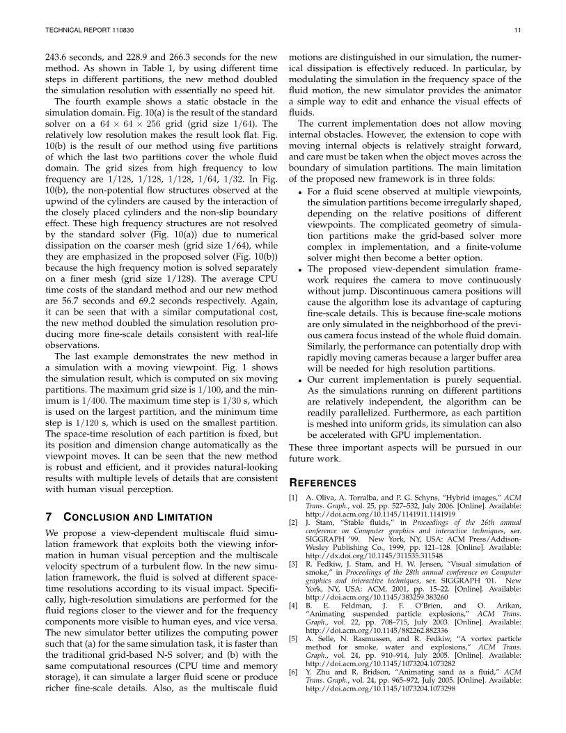
Fig. 10. Comparison of the standard solver and our newmethod with a static obstacle in the domain. (a) standardmethod, (b) our new method using 4 partitions withoutview control.

TECHNICAL REPORT 110830 10

Parameter Fig. 7(a) Fig. 7(b) Fig. 7(c) Fig. 9(a) Fig. 9(b) Fig. 9(c) Fig. 10(a) Fig. 10(b) Fig. 1highest resolution 1/128 1/128 1/128 1/200 1/400 1/400 1/64 1/128 1/400

avg. time per frame 45.1s 33.6s 35.5s 243.6s 228.9s 266.3s 56.7s 69.2s 328.0sspeedup percentage N/A 25.5% 23.3% N/A 6% -9.3% N/A -22% N/A

component num. N/A 6 6 N/A 5 5 N/A 5 5max down sample rate N/A 2 2 N/A 4 4 N/A 4 4

view control N/A No No N/A Yes Yes N/A Yes YesEMD interval N/A 10 10 N/A 10 15 N/A 20 5

editing N/A No Yes N/A No No N/A No No

TABLE 1Simulation parameters and performance.

using the new method with six simulation partitions allcovering the whole fluid domain. The first five partitionsare meshed as 128 × 256 × 128, and the last partition ismeshed as 64× 128× 64. All six partitions use the sametime step in their simulations, and the EMD is performedevery 10 frames to update the velocity spectrum. Com-paring Figs. 7(a-b), it is observed that the new methodproduces the correct result with more fine-scale features.This is because the new method separates differentfrequency components and solves them on differentpartitions, and by doing so, the numerical dissipationis effectively reduced. For each time step, the averageCPU time cost is 45.1 seconds in the standard N-S solver,and 33.6 for our new method. Without view control, thenew method is about 25% faster than the standard gridsolver. This is because (a) the sixth partition is solved onthe coarse grid; and (b) the first five partitions do nothave any body force and as a result, their simulationsconverge very fast, typically within 5 iterations. How-ever, the standard N-S solver uses the fine grid and ineach time step it takes 50 - 80 iterations to converge to theerror threshold 10−5. Fig. 7(c) shows a frequency editingresult, where the first three components are amplified bya factor 5, the next two components by 2, and the lastcomponent accordingly attenuated. It can be seen thatmore fine-scale turbulence details are achieved while theglobal motion of the plume (dominated by the lowerfrequency components) is accurately retained, which isimportant for practical editing.

Our new method assumes that the low frequencycomponents of a velocity field can be simulated oncoarse grids to save computational cost. This is verifiedin Fig. 8, where a plume is developed in a veloc-ity field that only contains low frequency components.Figs. 8(a-c) are the results obtained using a fine grid(128× 256× 128), and Figs. 8(d-f) are solved on a coarsegrid (64× 128× 64). The two groups of results are verysimilar up to frame 8 and they become more differentas the simulation continues. This observation confirmsthat the low frequency components of a velocity fielddo generate high frequency motions as time goes, butthese newly generated high frequency components areneglectable in the beginning period, during which thefluid motion can be well captured by using a coarsegrid. Therefore, we choose different grid resolutions toeconomically simulate different frequency components,

and periodically recompute the velocity spectrum toadjust the frequency-component allocation and ensurethat every frequency component is always simulatedusing the right grid resolution.

The third example examines the effect of view-dependent partitioning. The viewpoint is fixed inside thefluid domain. Fig. 9(a) shows the result obtained usingthe standard N-S solver on a 200×200×400 grid (grid size1/200). It can be seen that all four plumes are capturedat the same resolution, and the nearest plume to theviewer is lack of fine-scale details, which makes the scenelook unnatural. Fig. 9(b) shows the result obtained usingthe new method. It can be seen that different levelsof details are obtained in the scene, with more fine-scale features captured for plumes closer to the viewer.Five simulation partitions with different dimensions anddifferent grid sizes are used in the simulation. The firstfour partitions only cover approximately half depth ofthe scene and the fifth partition covers the whole fluiddomain. The grid sizes are 1/400, 1/400, 1/200, 1/200and 1/100, respectively. As small grid sizes are only usedon small partitions while larger partitions using largergrid sizes, the total memory used in the new method issimilar to the standard solver. Fig. 9(c) shows the resultof the new method using another set of parameters.In contrast to (b), the forth partition covers the wholedomain, and the EMD interval increases to 15. Fig.9(c) has some stair-like artifacts at the bottom of eachplume. These artifacts are partially caused by the largerinterval between adjacent EMD operations. Specifically,at a fixed frequency, the smoke source is added into thesimulation as a cylindrical smoke density field togetherwith some buoyancy forces. As the buoyancy force isonly added to the lowest frequency component in oursimulation framework (see Eqn.(8)), the smoke sourceis directly linked to the lowest frequency component.When the EMD interval increases, it takes longer tomix the velocity fields at different frequencies. Thus,the newly added smoke mainly moves with the lowestfrequency component at the initial stage, and producessome stair-like artifacts. This kind of artifacts can also beobserved in the standard solver when a strong smokesource is used in the simulation. In general, this typeof artifacts can be effectively removed by adjustingthe strength of the smoke source. For each time step,the average CPU time cost for the standard solver is

TECHNICAL REPORT 110830 11

243.6 seconds, and 228.9 and 266.3 seconds for the newmethod. As shown in Table 1, by using different timesteps in different partitions, the new method doubledthe simulation resolution with essentially no speed hit.

The fourth example shows a static obstacle in thesimulation domain. Fig. 10(a) is the result of the standardsolver on a 64 × 64 × 256 grid (grid size 1/64). Therelatively low resolution makes the result look flat. Fig.10(b) is the result of our method using five partitionsof which the last two partitions cover the whole fluiddomain. The grid sizes from high frequency to lowfrequency are 1/128, 1/128, 1/128, 1/64, 1/32. In Fig.10(b), the non-potential flow structures observed at theupwind of the cylinders are caused by the interaction ofthe closely placed cylinders and the non-slip boundaryeffect. These high frequency structures are not resolvedby the standard solver (Fig. 10(a)) due to numericaldissipation on the coarser mesh (grid size 1/64), whilethey are emphasized in the proposed solver (Fig. 10(b))because the high frequency motion is solved separatelyon a finer mesh (grid size 1/128). The average CPUtime costs of the standard method and our new methodare 56.7 seconds and 69.2 seconds respectively. Again,it can be seen that with a similar computational cost,the new method doubled the simulation resolution pro-ducing more fine-scale details consistent with real-lifeobservations.

The last example demonstrates the new method ina simulation with a moving viewpoint. Fig. 1 showsthe simulation result, which is computed on six movingpartitions. The maximum grid size is 1/100, and the min-imum is 1/400. The maximum time step is 1/30 s, whichis used on the largest partition, and the minimum timestep is 1/120 s, which is used on the smallest partition.The space-time resolution of each partition is fixed, butits position and dimension change automatically as theviewpoint moves. It can be seen that the new methodis robust and efficient, and it provides natural-lookingresults with multiple levels of details that are consistentwith human visual perception.

7 CONCLUSION AND LIMITATION

We propose a view-dependent multiscale fluid simu-lation framework that exploits both the viewing infor-mation in human visual perception and the multiscalevelocity spectrum of a turbulent flow. In the new simu-lation framework, the fluid is solved at different space-time resolutions according to its visual impact. Specifi-cally, high-resolution simulations are performed for thefluid regions closer to the viewer and for the frequencycomponents more visible to human eyes, and vice versa.The new simulator better utilizes the computing powersuch that (a) for the same simulation task, it is faster thanthe traditional grid-based N-S solver; and (b) with thesame computational resources (CPU time and memorystorage), it can simulate a larger fluid scene or producericher fine-scale details. Also, as the multiscale fluid

motions are distinguished in our simulation, the numer-ical dissipation is effectively reduced. In particular, bymodulating the simulation in the frequency space of thefluid motion, the new simulator provides the animatora simple way to edit and enhance the visual effects offluids.

The current implementation does not allow movinginternal obstacles. However, the extension to cope withmoving internal objects is relatively straight forward,and care must be taken when the object moves across theboundary of simulation partitions. The main limitationof the proposed new framework is in three folds:• For a fluid scene observed at multiple viewpoints,

the simulation partitions become irregularly shaped,depending on the relative positions of differentviewpoints. The complicated geometry of simula-tion partitions make the grid-based solver morecomplex in implementation, and a finite-volumesolver might then become a better option.

• The proposed view-dependent simulation frame-work requires the camera to move continuouslywithout jump. Discontinuous camera positions willcause the algorithm lose its advantage of capturingfine-scale details. This is because fine-scale motionsare only simulated in the neighborhood of the previ-ous camera focus instead of the whole fluid domain.Similarly, the performance can potentially drop withrapidly moving cameras because a larger buffer areawill be needed for high resolution partitions.

• Our current implementation is purely sequential.As the simulations running on different partitionsare relatively independent, the algorithm can bereadily parallelized. Furthermore, as each partitionis meshed into uniform grids, its simulation can alsobe accelerated with GPU implementation.

These three important aspects will be pursued in ourfuture work.

REFERENCES[1] A. Oliva, A. Torralba, and P. G. Schyns, “Hybrid images,” ACM

Trans. Graph., vol. 25, pp. 527–532, July 2006. [Online]. Available:http://doi.acm.org/10.1145/1141911.1141919

[2] J. Stam, “Stable fluids,” in Proceedings of the 26th annualconference on Computer graphics and interactive techniques, ser.SIGGRAPH ’99. New York, NY, USA: ACM Press/Addison-Wesley Publishing Co., 1999, pp. 121–128. [Online]. Available:http://dx.doi.org/10.1145/311535.311548

[3] R. Fedkiw, J. Stam, and H. W. Jensen, “Visual simulation ofsmoke,” in Proceedings of the 28th annual conference on Computergraphics and interactive techniques, ser. SIGGRAPH ’01. NewYork, NY, USA: ACM, 2001, pp. 15–22. [Online]. Available:http://doi.acm.org/10.1145/383259.383260

[4] B. E. Feldman, J. F. O’Brien, and O. Arikan,“Animating suspended particle explosions,” ACM Trans.Graph., vol. 22, pp. 708–715, July 2003. [Online]. Available:http://doi.acm.org/10.1145/882262.882336

[5] A. Selle, N. Rasmussen, and R. Fedkiw, “A vortex particlemethod for smoke, water and explosions,” ACM Trans.Graph., vol. 24, pp. 910–914, July 2005. [Online]. Available:http://doi.acm.org/10.1145/1073204.1073282

[6] Y. Zhu and R. Bridson, “Animating sand as a fluid,” ACMTrans. Graph., vol. 24, pp. 965–972, July 2005. [Online]. Available:http://doi.acm.org/10.1145/1073204.1073298

TECHNICAL REPORT 110830 12

[7] T. F. Dupont and Y. Liu, “Back and forth error compensation andcorrection methods for removing errors induced by uneven gra-dients of the level set function,” Journal of Computational Physics,vol. 190, pp. 311–324, 2003.

[8] J. Molemaker, J. M. Cohen, S. Patel, and J. Noh, “Lowviscosity flow simulations for animation,” in Proceedings ofthe 2008 ACM SIGGRAPH/Eurographics Symposium on ComputerAnimation, ser. SCA ’08. Aire-la-Ville, Switzerland, Switzerland:Eurographics Association, 2008, pp. 9–18. [Online]. Available:http://portal.acm.org/citation.cfm?id=1632592.1632595

[9] A. Selle, R. Fedkiw, B. Kim, Y. Liu, and J. Rossignac, “An uncon-ditionally stable maccormack method,” J. Sci. Comput., vol. 35, no.2-3, pp. 350–371, 2008.

[10] M. Lentine, W. Zheng, and R. Fedkiw, “A novel algorithmfor incompressible flow using only a coarse grid projection,”ACM Trans. Graph., vol. 29, pp. 114:1–114:9, July 2010. [Online].Available: http://doi.acm.org/10.1145/1778765.1778851

[11] J. Stam and E. Fiume, “Turbulent wind fields for gaseousphenomena,” in Proceedings of the 20th annual conference onComputer graphics and interactive techniques, ser. SIGGRAPH’93. New York, NY, USA: ACM, 1993, pp. 369–376. [Online].Available: http://doi.acm.org/10.1145/166117.166163

[12] A. Lamorlette and N. Foster, “Structural modeling offlames for a production environment,” ACM Trans. Graph.,vol. 21, pp. 729–735, July 2002. [Online]. Available:http://doi.acm.org/10.1145/566654.566644

[13] N. Rasmussen, D. Q. Nguyen, W. Geiger, and R. Fedkiw,“Smoke simulation for large scale phenomena,” ACM Trans.Graph., vol. 22, pp. 703–707, July 2003. [Online]. Available:http://doi.acm.org/10.1145/882262.882335

[14] R. Bridson, J. Houriham, and M. Nordenstam, “Curl-noise forprocedural fluid flow,” ACM Trans. Graph., vol. 26, July 2007.[Online]. Available: http://doi.acm.org/10.1145/1276377.1276435

[15] T. Kim, N. Thurey, D. James, and M. Gross, “Waveletturbulence for fluid simulation,” ACM Trans. Graph.,vol. 27, pp. 50:1–50:6, August 2008. [Online]. Available:http://doi.acm.org/10.1145/1360612.1360649

[16] R. Narain, J. Sewall, M. Carlson, and M. C. Lin, “Fast animationof turbulence using energy transport and procedural synthesis,”ACM Trans. Graph., vol. 27, pp. 166:1–166:8, December 2008.[Online]. Available: http://doi.acm.org/10.1145/1409060.1409119

[17] H. Schechter and R. Bridson, “Evolving sub-grid turbulencefor smoke animation,” in Proceedings of the 2008 ACMSIGGRAPH/Eurographics Symposium on Computer Animation,ser. SCA ’08. Aire-la-Ville, Switzerland, Switzerland:Eurographics Association, 2008, pp. 1–7. [Online]. Available:http://portal.acm.org/citation.cfm?id=1632592.1632594

[18] T. Pfaff, N. Thuerey, A. Selle, and M. Gross, “Syntheticturbulence using artificial boundary layers,” ACM Trans. Graph.,vol. 28, pp. 121:1–121:10, December 2009. [Online]. Available:http://doi.acm.org/10.1145/1618452.1618467

[19] T. Pfaff, N. Thuerey, J. Cohen, S. Tariq, and M. Gross, “Scalablefluid simulation using anisotropic turbulence particles,” ACMTrans. Graph., vol. 29, pp. 174:1–174:8, December 2010. [Online].Available: http://doi.acm.org/10.1145/1882261.1866196

[20] J.-C. Yoon, H. R. Kam, J.-M. Hong, S.-J. Kang, and C.-H. Kim,“Procedural synthesis using vortex particle method for fluidsimulation,” Comput. Graph. Forum, vol. 28, no. 7, pp. 1853–1859,2009.

[21] P. Mullen, K. Crane, D. Pavlov, Y. Tong, and M. Desbrun,“Energy-preserving integrators for fluid animation,” ACM Trans.Graph., vol. 28, pp. 38:1–38:8, July 2009. [Online]. Available:http://doi.acm.org/10.1145/1531326.1531344

[22] S. Elcott, Y. Tong, E. Kanso, P. Schroder, and M. Desbrun,“Stable, circulation-preserving, simplicial fluids,” ACMTrans. Graph., vol. 26, January 2007. [Online]. Available:http://doi.acm.org/10.1145/1189762.1189766

[23] B. E. Feldman, J. F. O’Brien, and B. M. Klingner,“Animating gases with hybrid meshes,” ACM Trans. Graph.,vol. 24, pp. 904–909, July 2005. [Online]. Available:http://doi.acm.org/10.1145/1073204.1073281

[24] F. Losasso, F. Gibou, and R. Fedkiw, “Simulating waterand smoke with an octree data structure,” ACM Trans.Graph., vol. 23, pp. 457–462, August 2004. [Online]. Available:http://doi.acm.org/10.1145/1015706.1015745

[25] J. Kim, I. Ihm, and D. Cha, “View-dependent adaptive animationof liquids,” ETRI Journal, vol. 28, pp. 697–708, December 2006.

[26] M. B. Nielsen, B. B. Christensen, N. B. Zafar, D. Roble,and K. Museth, “Guiding of smoke animations throughvariational coupling of simulations at different resolutions,”in Proceedings of the 2009 ACM SIGGRAPH/EurographicsSymposium on Computer Animation, ser. SCA ’09. NewYork, NY, USA: ACM, 2009, pp. 217–226. [Online]. Available:http://doi.acm.org/10.1145/1599470.1599499

[27] S. Barbara and M. Gross, “Two-scale particle simulation,” ACMTrans. on Graphics (Proc. SIGGRAPH), vol. 30, no. 4, pp. 72:1–72:8,2011.

[28] C. Horvath and W. Geiger, “Directable, high-resolutionsimulation of fire on the gpu,” ACM Trans. Graph.,vol. 28, pp. 41:1–41:8, July 2009. [Online]. Available:http://doi.acm.org/10.1145/1531326.1531347

[29] M. Lesieur, O. Mtais, and P. Comte, Large-Eddy Simulations ofTurbulence. Cambridge University Press, 2005.

[30] M. Wicke, M. Stanton, and A. Treuille, “Modular bases for fluiddynamics,” ACM Trans. Graph., vol. 28, pp. 39:1–39:8, July 2009.[Online]. Available: http://doi.acm.org/10.1145/1531326.1531345

[31] N. Huang, Z. Shen, S. Long, M. Wu, H. Shih, Q. Zheng, N. Yen,C. Tung, and H. Liu, “The empirical mode decomposition andthe Hilbert spectrum for nonlinear and non-stationary time seriesanalysis,” PROCEEDINGS OF THE ROYAL SOCIETY OF LON-DON SERIES A-MATHEMATICAL PHYSICAL AND ENGINEER-ING SCIENCES, vol. 454, no. 1971, pp. 903–995, MAR 8 1998.

[32] N. Huang and S. Shen, The Hilbert-Huang Transform and Its Appli-cations. World Scientific Publishing Company, 2005.

[33] J. Nunes, Y. Bouaoune, E. Delechelle, O. Niang, and P. Bunel, “Im-age analysis by bidimensional empirical mode decomposition,”IMAGE AND VISION COMPUTING, vol. 21, no. 12, pp. 1019–1026, NOV 1 2003.

[34] K. Subr, C. Soler, and F. Durand, “Edge-preserving multiscaleimage decomposition based on local extrema,” ACM Trans.Graph., vol. 28, pp. 147:1–147:9, December 2009. [Online].Available: http://doi.acm.org/10.1145/1618452.1618493

[35] C. Damerval, S. Meignen, and V. Perrier, “A fast algorithmfor bidimensional EMD,” IEEE SIGNAL PROCESSING LETTERS,vol. 12, no. 10, pp. 701–704, OCT 2005.

[36] Z. Liu and S. Peng, “Boundary Processing of bidimensional EMDusing texture synthesis,” IEEE Signal Processing Letters, vol. 12,no. 1, pp. 33–6, January 2005.

[37] P. Goswami, P. Schlegel, B. Solenthaler, and R. Pajarola,“Interactive sph simulation and rendering on the gpu,” inProceedings of the 2010 ACM SIGGRAPH/Eurographics Symposiumon Computer Animation, ser. SCA ’10. Aire-la-Ville, Switzerland,Switzerland: Eurographics Association, 2010, pp. 55–64. [Online].Available: http://dl.acm.org/citation.cfm?id=1921427.1921437

[38] L. D. Landau and E. Lifshitz, Fluid Mechanics, Second Edition:Volume 6 (Course of Theoretical Physics). Butterworth-Heinemann,1987.

[39] M. Pharr and G. Humphreys, Physically Based Rendering : FromTheory to Implementation. Morgan Kaufmann, August 2004.