continuum models in scale dependent plasticitywieners/gradientplasticity.pdf · karlsruhe institute...

Karlsruhe Institute of Technology

KIT – University of the State of Baden-Württemberg and National Research Center of the Helmholtz Association www.kit.edu

Continuum Models in Scale Dependent PlasticityAnalytical and Numerical Aspects

Christian Wieners

Institut für Angewandte und Numerische Mathematik, Karlsruhe

Karlsruhe Institute of TechnologyOutline

1. A Remark on Multiscale Plasticity

2. Generalized Standard Materials in Strain-Gradient Plasticity

3. Approximation of Strain-Gradient Plasticity

4. Algorithms in Strain-Gradient Plasticity

5. Results for Strain-Gradient Plasticity

Cooperations with ...

P. Neff (Essen), K. Chełminski (Warschau)B. Wohlmuth (München), D. Reddy (Capetown)W. Müller, A. Sydow, M. Sauter, D. Maurer (Karlsruhe)

1

Karlsruhe Institute of TechnologyDefects and Dislocations in a Single Crystal

Dislocations are micro-structuralline defects in the atomic latticeof a crystalline material alongwhich the crystallographicstructure is disturbed.

en.wikipedia.org/wiki/Dislocation

www.tf.uni-kiel.de/matwis/amat Weertman and Weertman 19822

Karlsruhe Institute of TechnologyDislocation Densities in a Single Crystal

We consider a single crystal with a finite set of slip systems A, determined by theslip direction sssα ∈ R3 and the slip-plane normal mmmα ∈ R3 for all α ∈ A.

Classical continuum theory of dislocationsThe displacement gradient can be decomposed into elastic and plastic part, i.e.,∇uuu = hhhe +hhhp. The dislocation density GGG is determined by∫

SGGGmmmda =

∫∂S

hhhpds ,

where S is a surface with normal mmm and ∂S is a dislocation loop, i.e., GGG = curlhhhp.

Constitutive setting in Crystal PlasticityWithin single crystal plasticity, the plastic distortion is of the form

hhhp(γγγ) = ∑αγ

α sssα ⊗mmmα ,

where γα is the plastic slip in the slip system α. This gives the macroscopicBurgers tensor and the edge and screw dislocation densities

GGG = curlhhhp = ∑α(∇γ

α ×mmmα )⊗sssα = ∑αρedge(mmmα ×sssα )⊗sssα + ρsrewsssα ⊗sssα .

Here we follow the monograph of Gurtin, Leele, Anand 2009.3

Karlsruhe Institute of TechnologyMaterials with Memory

We consider displacements

uuu : [0,T ]×Ω−→ R3

of a material with internal variables

zzz : [0,T ]×Ω−→ RN .

We assume that the free energy is of the form

Ψ(uuu,zzz) =∫

Ωψ(x ,∇u(x),z(x),∇z(x))dx

and the total energy is given

E (t ,uuu,zzz) = Ψ(uuu,zzz)−〈`(t),uuu〉 ,with the load functional 〈`(t),vvv〉=

∫Ω bbb(t) ·vvv dx +

∫ΓN

tttN (t) ·vvv da.

The plastic evolution is determined by a dissipation distance R.

Let VVV ⊂ H1(Ω,R3) and ZZZ ⊂ H1(Ω,RN ) are suitable spaces for (infinitesimal)displacements and internal variables, respectively. For simplicity, we assume thathomogeneous boundary conditions are included in the spaces.

4

Karlsruhe Institute of TechnologySmall Strain Plasticity

Within the infinitesimal setting we consider the following linear constitutiverelations: depending on the deformation we define the strain

εεε = sym(∇uuu) : [0,T ]×Ω−→ Sym(3)

and the plastic strain depending on the internal variables

εεεp(zzz) : [0,T ]×Ω−→ Sym(3) .

We assume that the free energy is of the form

Ψ(uuu,zzz) = Ψelastic(εεε(uuu)−εεε

p(zzz))

+ Ψdefect(zzz) ,

where the elastic energy is given by

Ψelastic(εεεe) =12

∫Ω

εεεe : C : εεε

edx .

The plastic evolution is determined by a convex dissipation functional

R : ZZZ −→ R∪∞ .Equivalently, the plastic evolution is determined by the plastic potential

χ : ZZZ ∗ −→ R∪∞defined by duality χ = R∗, i.e., χ(yyy) = supzzz∈ZZZ 〈yyy ,zzz〉−R(zzz).

5

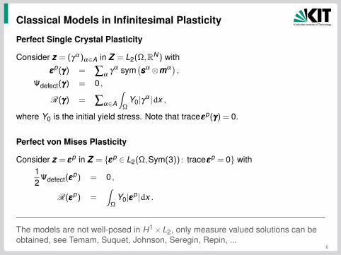
Karlsruhe Institute of TechnologyClassical Models in Infinitesimal Plasticity

Perfect Single Crystal Plasticity

Consider zzz = (γα )α∈A in ZZZ = L2(Ω,RN ) with

εεεp(γγγ) = ∑α

γα sym

(sssα ⊗mmmα

),

Ψdefect(γγγ) = 0 ,

R(γγγ) = ∑α∈A

∫Ω

Y0|γα |dx ,

where Y0 is the initial yield stress. Note that traceεεεp(γγγ) = 0.

Perfect von Mises Plasticity

Consider zzz = εεεp in ZZZ = εεεp ∈ L2(Ω,Sym(3)) : traceεεεp = 0 with12

Ψdefect(εεεp) = 0 ,

R(εεεp) =∫

ΩY0|εεεp|dx .

The models are not well-posed in H1×L2, only measure valued solutions can beobtained, see Temam, Suquet, Johnson, Seregin, Repin, ...

6

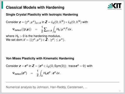
Karlsruhe Institute of TechnologyClassical Models with Hardening

Single Crystal Plasticity with Isotropic Hardening

Consider zzz = (γα ,µα )α∈A in ZZZ = L2(Ω,RN )×L2(Ω,RN ) with

Ψdefect((γγγ,µµµ)

)=

12 ∑α∈A

∫Ω

H0 |µα |2 dx ,

where H0 > 0 is the hardening modulus.We set domR = (γα ,µα ) ∈ZZZ : |γα | ≤ µα.

Von Mises Plasticity with Kinematic Hardening

Consider zzz = εεεp in ZZZ = εεεp ∈ L2(Ω,Sym(3)) : traceεεεp = 0 with

Ψdefect(εεεp) =

12

∫Ω

H0 εεεp : εεε

p dx .

Numerical analysis by Johnson, Han-Reddy, Carstensen, ...7

Karlsruhe Institute of TechnologyRepresentative Models in Strain Gradient Plasticity

Energy in a Single Crystal including Dislocation Densities ∇γα ×mmmα

Consider zzz = (γα ,µα )α∈A in ZZZ ⊂ H1(Ω,RN )×L2(Ω,RN ) with

Ψdefect((γγγ,µµµ)

)=

12 ∑α∈A

∫Ω

H0|µα |2 dx +∫

ΩL0|∇γ

α ×mmmα |2 dx ,

where L0 > 0 is the length scale parameter.

Energy including the Burgers Tensor curlhhhp

Consider zzz = hhhp in ZZZ = H(curl,Ω)3 with

Ψdefect(hhhp) =

12

∫Ω

H0hhhp : hhhp dx +∫

ΩL0 curlhhhp : curlhhhp dx

and εεεp(zzz) = symdevhhhp.

Studied by Gurtin, Needleman, Geers, Reddy, Svendson, Steinmann, Forest, ...

8

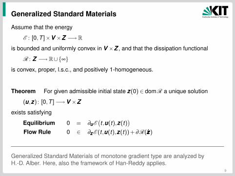
Karlsruhe Institute of TechnologyGeneralized Standard Materials

Assume that the energy

E : [0,T ]×VVV ×ZZZ −→ R

is bounded and uniformly convex in VVV ×ZZZ , and that the dissipation functional

R : ZZZ −→ R∪∞

is convex, proper, l.s.c., and positively 1-homogeneous.

Theorem For given admissible initial state zzz(0) ∈ domR a unique solution

(uuu,zzz) : [0,T ]−→VVV ×ZZZ

exists satisfying

Equilibrium 0 = ∂uuuE(t ,uuu(t),zzz(t)

)Flow Rule 0 ∈ ∂zzzE (t ,uuu(t),zzz(t)) + ∂R(zzz)

Generalized Standard Materials of monotone gradient type are analyzed byH.-D. Alber. Here, also the framework of Han-Reddy applies.

9

Karlsruhe Institute of TechnologyConjugated Variables and Duality

The conjugated variables (TTT ,yyy) for (uuu,zzz) are given by

TTT = ∂εεεe Ψelastic(εεε

e)yyy = −∂zzzΨ(uuu,zzz) ∈ZZZ ∗

This gives TTT = C : (εεε(uuu)−εεεp(zzz)) ∈ L2(Ω,Sym(3)).

For generalized standard materials, we obtain:

Macroscopic Balance Equation∫Ω

TTT : εεε(vvv)dx = 〈`(t),vvv〉 for all vvv ∈VVV

Microscopic Balance Equation

〈yyy ,www〉 =∫

ΩTTT : εεε

p(www)dx−〈∂ Ψdefect(zzz),www〉 for all www ∈ZZZ

Flow Rule

zzz ∈ ∂ χ(yyy) ⇐⇒ yyy ∈ ∂R(zzz)

10

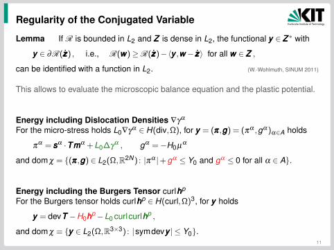
Karlsruhe Institute of TechnologyRegularity of the Conjugated Variable

Lemma If R is bounded in L2 and ZZZ is dense in L2, the functional yyy ∈ZZZ ∗ with

yyy ∈ ∂R(zzz) , i.e., R(www)≥R(zzz)−〈yyy ,www − zzz〉 for all www ∈ZZZ ,

can be identified with a function in L2. (W.-Wohlmuth, SINUM 2011)

This allows to evaluate the microscopic balance equation and the plastic potential.

Energy including Dislocation Densities ∇γα

For the micro-stress holds L0∇γα ∈ H(div,Ω), for yyy = (πππ,ggg) = (πα ,gα )α∈A holds

πα = sssα ·TTTmmmα + L0∆γ

α , gα =−H0µα

and dom χ = (πππ,ggg) ∈ L2(Ω,R2N ) : |πα |+ gα ≤ Y0 and gα ≤ 0 for all α ∈ A.


For the Burgers tensor holds curlhhhp ∈ H(curl,Ω)3, for yyy holds

yyy = devTTT −H0hhhp−L0 curlcurlhhhp ,

and dom χ = yyy ∈ L2(Ω,R3×3) : |symdevyyy | ≤ Y0.11

Karlsruhe Institute of TechnologyPoint-wise Complementarity

The regularity of yyy =−∂zzzΨ(uuu,zzz) allows for a point-wise evaluation of the flow rule

zzz ∈ ∂ χ(yyy) ⇐⇒ yyy ∈ ∂R(zzz)

Energy including Dislocation Densities ∇γα

For yyy = (πα ,gα ) = (τα −ζ α ,−H0µα ) with τα = sssα ·TTTmmmα and ζ α =−L0∆γα holds

(γα , µ

α ) = λα (sgnπ

α ,1)

and the complementarity condition for the consistency parameters λ α

λα ≥ 0 , |πα |+ gα −Y0 ≤ 0 ,

(|πα |+ gα −Y0

)λ

α = 0 .


For yyy = devTTT −βββ with βββ = H0hhhp−L0 curlcurlhhhp holds

εεεεεεεεεp = γ

devTTT −βββ

|devTTT −βββ |and the complementarity condition for the consistency parameters λ

|devTTT −βββ | ≤ Y0 , λ ≥ 0 , λ (|devTTT −βββ |−Y0) = 0 .

12

Karlsruhe Institute of TechnologyIncremental Infinitesimal Plasticity

Let 0 = t0 < t1 < t2 < · · · be a time series. In step n, find (uuun,zzzn) ∈VVV ×ZZZ with

0 = ∂uuuE(tn,uuun,zzzn)

0 ∈ ∂zzzE (tn,uuun,zzzn) + ∂R(4zzzn) ⇐⇒ 4zzzn ∈ ∂ χ(−∂zzzE (tn,uuun,zzzn)

)for given (uuun−1,zzzn−1), where 4zzzn = zzzn−zzzn−1.

The incremental solution (uuun,zzzn) ∈VVV ×ZZZ is the unique minimizer of

4J n(uuu,zzz) = Ψ(uuu,zzz) +R(zzz−zzzn−1)−〈`n,uuu〉 .

Let VVV h×ZZZ h ⊂VVV ×ZZZ and let Πh be the L2 projection onto piecewise constants.

The fully discrete solution (uuun,h,zzzn,h) ∈VVV h×ZZZ h is the unique minimizer of

4J n,h(uuuh,zzzh) = Ψh(uuuh,zzzh) +Rh(zzzh−zzzn−1,h)−〈`n,uuun,h〉 ,

where Ψh(uuu,zzz) = Ψelastic(εεε(uuu)−εεεp(Πhzzz)) + Ψdefect(zzz) and Rh(zzz) = R(Πhzzz).

13

Karlsruhe Institute of TechnologyPrimal-Dual Constraint Convex Minimization

Let (uuun,h,zzzn,h) ∈VVV h×ZZZ h be the discrete solution. Define

TTT n,h = C : (εεε(uuun,h)−εεεp(Πhzzzn,h)) ,

τττn,h = −Πh∂ Ψ∗elastic(TTT n,h) .

Lemma If ΠhZZZ h = BBBh ⊂ L2(Ω,RN ), a discrete ’back stress’ βββ n,h ∈BBBh existssatisfying

〈βββ n,h,wwwh〉= 〈∂ Ψdefect(zzzn,h),wwwh〉 , wwwh ∈ZZZ h .

If inf‖βββ h‖0=1

sup‖zzzh‖ZZZ =1

〈βββ h,zzzh〉 ≥ c0 > 0, βββ n,h is unique. (W.-Wohlmuth, SINUM 2011)

The primal-dual solution (uuun,h,zzzn,h,βββ n,h) is characterized bythe linear Macroscopic Balance Relation

〈TTT n,h,εεε(vvvh)〉= 〈`n,vvvh〉 , vvvh ∈VVV h ,

the linear Microscopic Balance Relation〈βββ n,h,wwwh〉= 〈∂ Ψdefect(zzz

n,h),wwwh〉 , wwwh ∈ZZZ h

the convex Plastic Admissibilityτττ

n,h ∈ dom χ +βββn,h .

14

Karlsruhe Institute of TechnologyThe Radial Return

The radial return allows to compute TTT n,h and Πh4zzzn,h from

TTT trial = C : (εεε(uuun,h)−εεεp(Πhzzzn−1,h)) ,

yyy trial = yyyn−1,h−βββn,h

locally. This defines also the plastic response Πhzzzn,h = Rn(uuun,h,βββ n,h).

Theorem The primal-dual solution (uuun,h,zzzn,h,βββ n,h) is the unique solution of thenonlinear equation⟨

C :(εεε(uuun,h)−εεε

p(Rn(uuun,h,βββ n,h))),vvvh⟩−〈`n,vvvh〉 = 0 , vvvh ∈VVV h ,

−〈βββ n,h,wwwh〉+ 〈∂ Ψdefect(zzzn,h),wwwh〉 = 0 , wwwh ∈ZZZ h ,

〈Rn(uuun,h,βββ n,h),ηηηh〉−〈zzzn,h,ηηηh〉 = 0 , ηηηh ∈BBBh .

This nonlinear system is the critical point of an incremental saddle pointfunctional. Thus, the linearization is symmetric but indefinite.The system is strongly semi-smooth and a generalized Newton method issuperlinear convergent.For bubble-enhanced finite elements optimal order convergence estimates canbe provided.

15

Karlsruhe Institute of TechnologyThe Radial Return for Single-Crystal Plasticity

For given ζζζ ∈ L2(Ω,RN ), let P(·, ·;ζζζ ) be the orthogonal projection onto

CCC(ζζζ ) =

(TTT ,ggg) ∈ L2(Ω,Sym(3))×L2(Ω,RN ) : ϕα (TTT ,ggg,ζζζ )≤ 0 , α = 1, ...,N

with respect to the metric induced by

‖(TTT ,ggg)‖2 =∫

Ω

(TTT : C−1 : TTT + H−1

0 ∑α|gα |2

)dx ,

where ϕα (TTT ,ggg,ζζζ ) = |TTT : NNNα −ζ α |+ gα −Y0 and NNNα = sym(sssα ⊗mmmα ).

For given (TTT trial,gggtrial), the projection is uniquely determined by the KKT system

0 = C−1(TTT −TTT trial) +∑αλ

α sgn(TTT : NNNα −ζα )NNNα ,

0 = H−10 (ggg−gggtrial) +λλλ ,

0≤ λλλ , ϕα (TTT ,ggg,ζζζ )≤ 0 , ∑α

λα

ϕα (TTT ,ggg,ζζζ ) = 0 .

The solution of the KKT system defines the radial return

(TTT ,ggg) = P(TTT trial,gggtrial;ζζζ )

and thus also the response function for the plastic slips.16

Karlsruhe Institute of TechnologyEnergy including Dislocation Densities: Results

Distribution of the plastic slips γα for a shear test with Ω = (0, lΩ)2× (0,3lΩ) andlΩ = 20 [µ]. The results for the slip planes 111, 111, 111, 1 11 coincide inthe slip directions 〈011〉, 〈110〉, 〈101〉 up to rotation and sign changing.(joint work with B. D. Reddy and B. I. Wohlmuth)

17

Karlsruhe Institute of TechnologyClassical Single-Crystal Plasticity: Results

Distribution of the plastic slips γα for a shear test with Ω = (0, lΩ)2× (0,3lΩ) andlΩ = 20 [µ]. The results for the slip planes 111, 111, 111, 1 11 coincide inthe slip directions 〈011〉, 〈110〉, 〈101〉 up to rotation and sign changing.(joint work with B. D. Reddy and B. I. Wohlmuth)

18


192 cells1536 cells

12288 cells98304 cells

t0.080.060.040.020

t ‖TTT‖SSS‖εεε(uuu)‖EEE

0.04

0.035

0.03

0.025

0.02

0.015

0.01

0.005

0

Convergence in space of the stress-strain relation for the shear test.

(joint work with B. D. Reddy and B. I. Wohlmuth)

19

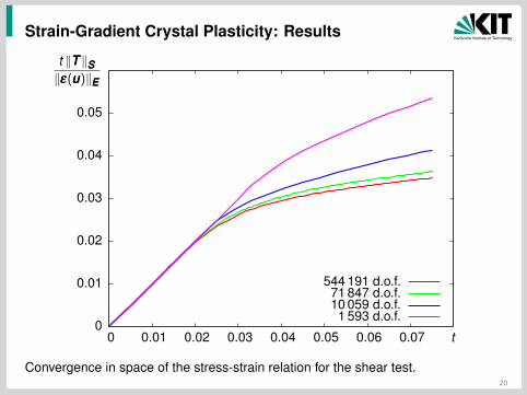
Karlsruhe Institute of TechnologyStrain-Gradient Crystal Plasticity: Results

1 593 d.o.f.10 059 d.o.f.71 847 d.o.f.

544 191 d.o.f.

t0.070.060.050.040.030.020.010


0.05

0.04

0.03

0.02

0.01

0

Convergence in space of the stress-strain relation for the shear test.


20


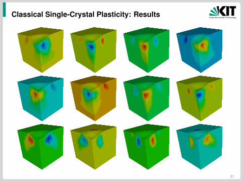
Distribution of the plastic slip γα for an indentation test.(joint work with B. D. Reddy and B. I. Wohlmuth)

21

Karlsruhe Institute of TechnologyStrain-Gradient Crystal Plasticity: Results

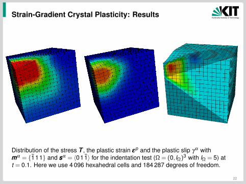
Distribution of the stress TTT , the plastic strain εεεp and the plastic slip γα withmmmα = 111 and sssα = 〈011〉 for the indentation test (Ω = (0, lΩ)3 with lΩ = 5) att = 0.1. Here we use 4 096 hexahedral cells and 184 287 degrees of freedom.

22


lΩ = 5lΩ = 7.5lΩ = 10lΩ = 20lΩ = 30lΩ = ∞

t0.080.060.040.020


0.05

0.04

0.03

0.02

0.01

0

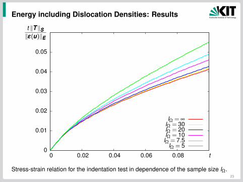
Stress-strain relation for the indentation test in dependence of the sample size lΩ.


23


lΩ = 5lΩ = 7.5lΩ = 10lΩ = 20lΩ = 30lΩ = ∞

0.10.080.060.040.020

‖ζζζ‖∞

6000

5000

4000

3000

2000

1000

0

Evolution of the back stress for the indentation test depending on lΩ.


24

Karlsruhe Institute of TechnologyEnergy including Burgers Tensor: Macroscopic Limit

Dependence on the length scale parameter L0 = µS l20 .

l0 0.1 0.01 0.001 0.0001 0Example 1 ‖TTT h‖SSS 2.0543 2.0881 2.1109 2.1121 2.1122

‖hhhph‖QQQ 0.4864 0.3834 0.2973 0.2888 0.2884

‖εεε(uuuh)‖EEE 24.73 29.29 41.83 42.59 42.61‖curlhhhp

h‖0 0.0106 0.0751 0.300 0.364Example 2 ‖TTT h‖SSS 2.5231 2.5687 2.6317 2.6374 2.6382

‖hhhph‖QQQ 1.1145 0.9786 0.6899 0.6551 0.6493

‖εεε(uuuh)‖EEE 78.75 83.96 91.73 92.51 92.67‖curlhhhp

h‖0 0.00566 0.154 0.703 1.294 25

Karlsruhe Institute of TechnologyEnergy including Burgers Tensor: Convergence

Convergence history (up to ε ≤ 10−9) of the semi-smooth Newton method.

k ρ0 ρ1 ρ2 ρ3 ρ4 ρ5 ρ6 ρ7 ρ8 ρ9

0 160.3 16.4 0.06 10−6 ε

1 89.6 46.2 17.24 0.971 0.002 ε

2 47.1 39.5 13.11 2.842 0.072 2 ·10−5 ε

3 24.1 12.4 11.68 8.649 7.727 1.572 0.19 0.0011 ε

4 12.2 6.7 6.13 4.661 4.585 1.235 0.15 0.0016 2 ·10−5 ε

Convergence for successive uniform refinements of the displacementat a test point x = (0,0,7) and for the stress maximum.

level k d.o.f. # cells # plastic cells |uuuh(zzz)| ‖TTT h‖∞

0 1 426 50 8 0.0167 581.641 8 903 400 77 0.0158 879.082 62 419 3 200 836 0.0192 1161.383 466 499 25 600 7 122 0.0214 1506.844 3 605 251 204 800 60 622 0.0228 1941.87

(joint work with B. I. Wohlmuth)

26

Karlsruhe Institute of TechnologyEnergy including the Burgers Tensor: Results

stress TTT n,h27

continuum models in scale dependent plasticitywieners/gradientplasticity.pdf · karlsruhe institute...

Documents