Research ArticleFluid Discrimination Based on Frequency-Dependent AVOInversion with the Elastic Parameter Sensitivity Analysis

Pu Wang ,1 Jingye Li ,1 Xiaohong Chen,1 Kedong Wang,1 and Benfeng Wang 2

1State Key Laboratory of Petroleum Resources and Prospecting, National Engineering Laboratory for Offshore Oil Exploration,China University of Petroleum-Beijing, Beijing 102249, China2Tongji University, State Key Laboratory of Marine Geology, School of Ocean and Earth Science, Institute for Advanced Study,Shanghai 200092, China

Correspondence should be addressed to Jingye Li; ljy3605@sina.com

Received 15 August 2019; Revised 15 October 2019; Accepted 21 November 2019; Published 18 December 2019

Academic Editor: Mohammad Sarmadivaleh

Copyright © 2019 PuWang et al. This is an open access article distributed under the Creative Commons Attribution License, whichpermits unrestricted use, distribution, and reproduction in any medium, provided the original work is properly cited.

Fluid discrimination is an extremely important part of seismic data interpretation. It plays an important role in the refineddescription of hydrocarbon-bearing reservoirs. The conventional AVO inversion based on Zoeppritz’s equation shows potentialin lithology prediction and fluid discrimination; however, the dispersion and attenuation induced by pore fluid are not fullyconsidered. The relationship between dispersion terms in different frequency-dependent AVO equations has not yet beendiscussed. Following the arguments of Chapman, the influence of pore fluid on elastic parameters is analyzed in detail. We findthat the dispersion and attenuation of Russell fluid factor, Lamé parameter, and bulk modulus are more pronounced than thoseof P-wave modulus. The Russell fluid factor is most prominent among them. Based on frequency-dependent AVO inversion, theuniform expression of different dispersion terms of these parameters is derived. Then, incorporating the P-wave difference withthe dispersion terms, we obtain new P-wave difference dispersion factors which can identify the gas-bearing reservoir locationbetter compared with the dispersion terms. Field data application also shows that the dispersion term of Russell fluid factor isoptimal in identifying fluid. However, the dispersion term of Russell fluid factor could be unsatisfactory, if the value of theweighting parameter associated with dry rock is improper. Then, this parameter is studied to propose a reasonable setting range.The results given by this paper are helpful for the fluid discrimination in hydrocarbon-bearing rocks.

1. Introduction

Rock physics is an effective tool for studying reservoir petro-physical properties from elastic and anelastic parameters [1].Effective elastic media theory and poroelasticity theory arevery important components of rock physics theories. The dif-ference is that whether the mobility of pore fluid is consid-ered or not [1]. The former considers the effects of poregeometry [2–4], instead of the effects of fluid flow on velocity.The Biot-Gassmann theory [5] is the research basis of mostporoelasticity theories which are used to study the wavepropagation in fluid-saturated rocks. The Gassmann theo-rem is proved to be valid for many types of rocks [6, 7],and it is used to predict P- and S-wave velocities in the low-frequency band [8, 9]. Due to the influence of pore fluid,

dispersion and attenuation occur in the elastic parametersof rocks [10–12]. It is the same in the seismic frequency band,and some researchers have described the dispersion andattenuation by rock physics modeling. White proposed amodel for seismic wave attenuation which is caused by thepatchy saturation of two kinds of pore fluid [13]. The Whitemodel is extended afterward to be incorporated with Biot’stheory [14] or to characterize the complex pore structure[15]. Chapman et al. [16] presented a model which considersthe squirt flow related to cracks. This model is consistent withthe Gassmann’s relations at low frequency. Considering theanisotropy caused by the parallel arrangement of the cracks,Chapman [17] derived an anisotropic attenuation model.Wu et al. [18] gave three key assumptions: the model isconsistent with the Gassmann-Wood prediction, partial

HindawiGeofluidsVolume 2019, Article ID 8750127, 13 pageshttps://doi.org/10.1155/2019/8750127

saturation brings about higher attenuation value than fullsaturation, and the characteristic frequency on fluid mobilityfollows the theory of squirt flow. Based on these arguments,the Chapman model [16] is used to analyze the dispersionand attenuation of elastic parameters in the seismic fre-quency band in this paper, and the cracks are considered tobe randomly arranged.

Rock physics plays an important role in reservoir pre-diction and can be used to obtain subsurface petrophysicalproperties [19, 20]. The amplitude variation with offset(AVO) inversion is an effective method in reservoir inter-pretation and prediction [21–23]. The exact and approxi-mate equations of Zoeppritz’s equation are adopted forthe AVO inversion [24–26]. The approximate equationshave good linearity and clear physical meaning [27–30]and can be more effectively applied to reservoir prediction.Exact Zoeppritz’s equation is a nonlinear forward opera-tor, which may increase computation cost, while it is moresuitable for far offset information [31]. With the develop-ment of exploration and exploitation, the lithologic trapreservoir has drawn much attention, and accurate descrip-tion for hydrocarbon-bearing rocks is required. It bringshuge challenges to fluid discrimination. There are mainlytwo methods for fluid discrimination by incorporatingrock physics and seismic inversion [32]. One is to predictreservoir petrophysical properties directly by using theempirical or theoretical rock physics model [33]. Theother is to identify fluid indirectly by using elastic param-eters [34, 35]. The prediction precision of the formermethod is based on the accuracy of the rock physicsmodel, which is the quantitative interpretation method.The latter depends on the understanding of the relation-ship between petrophysical properties and elastic parame-ters, which is the qualitative interpretation method. TheAVO inversion shows a certain ability in lithology predic-tion and fluid discrimination [36, 37]. However, the elasticparameter inversion based on Zoeppritz’s equation doesnot consider the effect of dispersion and attenuationcaused by pore fluid. Wilson et al. proposed frequency-dependent AVO (FAVO) following the approximation ofSmith and Gidlow [38]. And the dispersion term usedfor fluid discrimination can be obtained by using FAVOinversion. The resolution of spectral decomposition canaffect the accuracy of FAVO inversion. Wu et al. [39]and Luo et al. [40] used the smooth pseudo Wigner-Ville distribution and inverse spectral decomposition forthe time-frequency analysis, respectively, to enhance theresolution and accuracy of FAVO inversion results. Inorder to identify the hydrocarbon-bearing reservoir accu-rately, more sensitive frequency-dependent fluid factorneeds to be studied [41]. Zhang et al. proposed a new fluidfactor following the approximation of Russell et al. [42].Chen et al. [43] and Wang et al. [44] suggested P-wavedifference dispersion factor (PDDF) and bulk modulus dif-ference dispersion factor (MDDF) to identify pore fluid,respectively.

In this paper, the attenuation and dispersion of elasticparameters are analyzed in detail to identify which is moredispersion sensitive. The results show that the pore fluid

can bring more attenuation to Russell fluid factor, Laméparameter, and bulk modulus, compared with P-wave veloc-ity. This is critical for us to decide which dispersion term tobe used in the FAVO inversion. In addition, the applicabilityof Russell AVO approximation is analyzed, and a more rea-sonable range of the pending parameter is given, which canavoid a large deviation. Then, based on FAVO inversion,the dispersion terms and PDDFs related to Russell fluidfactor, Lamé parameter, and bulk modulus are derived.The PDDFs are superior to dispersion terms in identifyingthe gas-bearing reservoir. In order to improve the antinoiseability of the inversion, ℓ1 norm regularization term [45]is applied.

2. Theory and Method

The current study of fluid identification is based on the dis-persion and attenuation of elastic parameters. Therefore,the Chapman model [16] is used to analyze which parameteris more sensitive to the dispersion and attenuation inducedby the pore fluid. Then, the theories of sparse constrainedinversion spectral decomposition and frequency-dependentAVO inversion are summarized. In this section, the formulaof frequency-dependent AVO is rewritten with respect toother elastic parameters and the applicability of RussellAVO approximation is analyzed.

2.1. Dispersion and Attenuation Analysis of ElasticParameters. Chapman et al. [16] presented a frequency-dependent model which considers the wave-inducedexchange of fluids between pores and cracks, as well asbetween cracks. The cracks in this model are randomlyarranged without causing anisotropy. In the low-frequency limit, this model is consistent with the predictedresult by using the Gassmann equation. By correcting theisotropic elastic tensor of the material with the perturba-tion due to the presence of cracks and pores, it defines avalid expression:

Cijkl = C0ijkl λ, μð Þ − C1

ijkl λ, μ, ω, τ, ϕ, r, ε, κf� �

, ð1Þ

where C0ijklð•Þ is the isotropic elastic tensor without inclu-

sions and C1ijklð•Þ is the term affected by cracks and pores;

λ, μ, ω, τ, ϕ, r, ε, and κf are the Lamé parameter, shearmodulus, angular frequency, timescale parameter, porosity,crack aspect ratio, crack density, and fluid bulk modulus,respectively. The detailed expression of Cijkl is given byChapman et al. [46].

According to equation (1), we can get the elasticparameters influenced by frequency and fluid. Followingthe arguments of Chapman et al., the S-wave velocity alsohas attenuation and dispersion. This is because some ofthe cracks will necessarily have an orientation such thatthey will be compressed due to applied shear stress [47].The attenuation of S-wave velocity is smaller than thatof P-wave velocity in the Chapman model. To obtainattenuation characteristics of different elastic parameters,

2 Geofluids

other fluid-sensitive frequency-dependent elastic parame-ters are studied by removing the shear modulus from theP-wave modulus:

λ =M − 2μ,

K =M −43 μ,

f =M − γ2dryμ,

ð2Þ

where K , M, and f are the bulk modulus, P-wave modu-lus, and Russell fluid factor, respectively; γ2dry is theweighting parameter associated with the dry rock andγ2dry = ðVP/VSÞ2dry [35]; VP indicates P-wave velocity, andVS indicates S-wave velocity; subscript dry indicates thedry rock. In the FAVO inversion, the dispersion termswhich are induced by the pore fluid are related to theseparameters. Thus, these parameters are analyzed beforethe introduction of FAVO inversion.

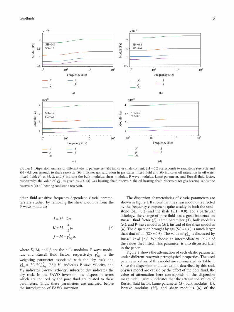
The dispersion characteristics of elastic parameters areshown in Figure 1. It shows that the shear modulus is affectedby the frequency component quite weakly in both the sand-stone (SH = 0:2) and the shale (SH = 0:8). For a particularlithology, the change of pore fluid has a great influence onRussell fluid factor (f ), Lamé parameter (λ), bulk modulus(K), and P-wave modulus (M), instead of the shear modulus(μ). The dispersion brought by gas (SG = 0:6) is much largerthan that of oil (SO = 0:6). The value of γ2dry is discussed byRussell et al. [35]. We choose an intermediate value 2.3 ofthe values they listed. This parameter is also discussed laterin the paper.

Figure 2 shows the attenuation of each elastic parameterunder different reservoir petrophysical properties. The usedparameter values of this model are summarized in Table 1.Since the dispersion and attenuation described by this rockphysics model are caused by the effect of the pore fluid, thevalue of attenuation here corresponds to the dispersionmagnitude. Figure 2 indicates that the attenuation values ofRussell fluid factor, Lamé parameter (λ), bulk modulus (K),P-wave modulus (M), and shear modulus (μ) of the

100 101 102 103

Frequency (Hz)

0.5

1

1.5

2

Mod

uli (

Pa)

×1010

SH=0.8SG=0.6

K𝜇

𝜆

Mf

(a)

100 101 102 103

×1010

Frequency (Hz)

0.5

1

1.5

2

Mod

uli (

Pa) SH=0.8

SO=0.6

K𝜇

𝜆

Mf

(b)

×1010

Frequency (Hz)

1

2

3

4

Mod

uli (

Pa)

K𝜇

𝜆

Mf

SG=0.6SH=0.2

100 101 102 103

(c)

×1010

Frequency (Hz)

1

2

3

4

Mod

uli (

Pa) SH=0.2

SO=0.6

100 101 102 103

K𝜇

𝜆

Mf

(d)

Figure 1: Dispersion analysis of different elastic parameters. SH indicates shale content, SH = 0:2 corresponds to sandstone reservoir andSH = 0:8 corresponds to shale reservoir; SG indicates gas saturation in gas-water mixed fluid and SO indicates oil saturation in oil-watermixed fluid; K , μ, M, λ, and f indicate the bulk modulus, shear modulus, P-wave modulus, Lamé parameter, and Russell fluid factor,respectively; the value of γ2dry is given as 2.3. (a) Gas-bearing shale reservoir; (b) oil-bearing shale reservoir; (c) gas-bearing sandstone

reservoir; (d) oil-bearing sandstone reservoir.

3Geofluids

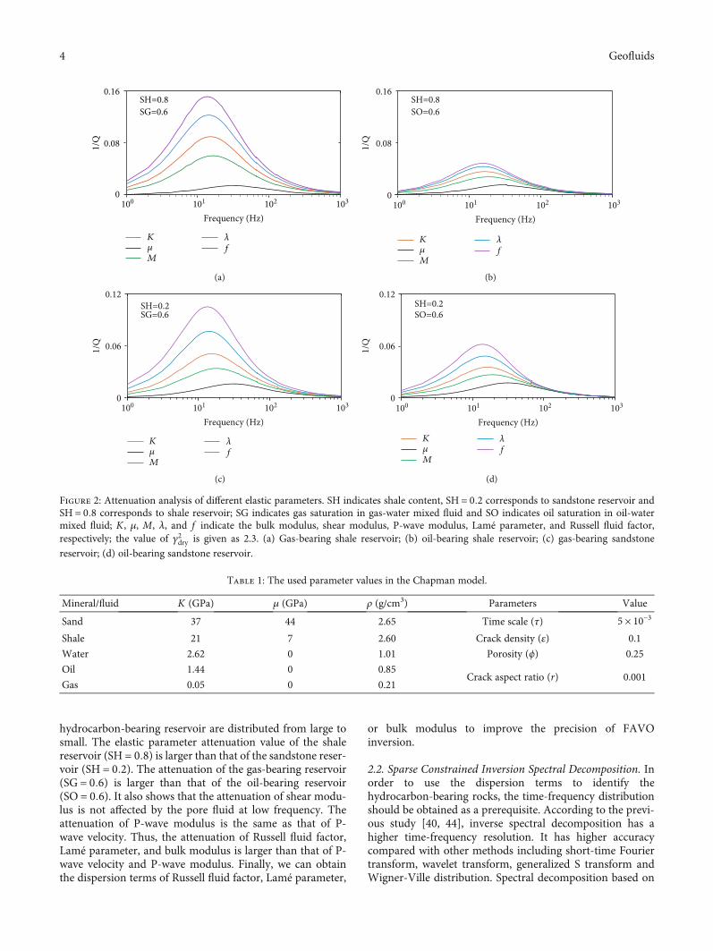
hydrocarbon-bearing reservoir are distributed from large tosmall. The elastic parameter attenuation value of the shalereservoir (SH = 0:8) is larger than that of the sandstone reser-voir (SH = 0:2). The attenuation of the gas-bearing reservoir(SG = 0:6) is larger than that of the oil-bearing reservoir(SO = 0:6). It also shows that the attenuation of shear modu-lus is not affected by the pore fluid at low frequency. Theattenuation of P-wave modulus is the same as that of P-wave velocity. Thus, the attenuation of Russell fluid factor,Lamé parameter, and bulk modulus is larger than that of P-wave velocity and P-wave modulus. Finally, we can obtainthe dispersion terms of Russell fluid factor, Lamé parameter,

or bulk modulus to improve the precision of FAVOinversion.

2.2. Sparse Constrained Inversion Spectral Decomposition. Inorder to use the dispersion terms to identify thehydrocarbon-bearing rocks, the time-frequency distributionshould be obtained as a prerequisite. According to the previ-ous study [40, 44], inverse spectral decomposition has ahigher time-frequency resolution. It has higher accuracycompared with other methods including short-time Fouriertransform, wavelet transform, generalized S transform andWigner-Ville distribution. Spectral decomposition based on

0.08

0.161/

Q

SG=0.6SH=0.8

0

Frequency (Hz)100 101 102 103

K𝜇

𝜆

Mf

(a)

0

0.08

0.16

1/Q

SO=0.6SH=0.8

Frequency (Hz)100 101 102 103

K𝜇

𝜆

Mf

(b)

0

0.06

0.12

1/Q

SG=0.6SH=0.2

K𝜇

𝜆

Mf

Frequency (Hz)100 101 102 103

(c)

0

0.06

0.12

1/Q

SO=0.6SH=0.2

Frequency (Hz)100 101 102 103

K𝜇

𝜆

Mf

(d)

Figure 2: Attenuation analysis of different elastic parameters. SH indicates shale content, SH = 0:2 corresponds to sandstone reservoir andSH = 0:8 corresponds to shale reservoir; SG indicates gas saturation in gas-water mixed fluid and SO indicates oil saturation in oil-watermixed fluid; K , μ, M, λ, and f indicate the bulk modulus, shear modulus, P-wave modulus, Lamé parameter, and Russell fluid factor,respectively; the value of γ2dry is given as 2.3. (a) Gas-bearing shale reservoir; (b) oil-bearing shale reservoir; (c) gas-bearing sandstone

reservoir; (d) oil-bearing sandstone reservoir.

Table 1: The used parameter values in the Chapman model.

Mineral/fluid K (GPa) μ (GPa) ρ (g/cm3) Parameters Value

Sand 37 44 2.65 Time scale (τ) 5 × 10−3

Shale 21 7 2.60 Crack density (ε) 0.1

Water 2.62 0 1.01 Porosity (ϕ) 0.25

Oil 1.44 0 0.85Crack aspect ratio (r) 0.001

Gas 0.05 0 0.21

4 Geofluids

sparse constrained inversion is thus used to obtain the high-resolution time-frequency distribution.

Using a dictionary of Ricker wavelets with different cen-tral frequencies, the seismic data can be decomposed intocorresponding frequency-dependent pseudoreflectivity. Theconvolutional model can be represented by a linear systemof equations [48], and the seismic trace s can be expressed as

s = W1 W2 ⋯ Wlð Þ

r1r2⋮

rl

0BBBBB@

1CCCCCA = Rm, ð3Þ

where Wi refers to the Ricker wavelet with central frequencyf i and ri refers to the corresponding pseudoreflectivitysequence; R indicates the dictionary of Ricker wavelets andm indicates the vector containing the pseudoreflectivitysequences [40].

The ℓ1 norm regularization term can be applied toobtain a high-resolution result [45, 49] and it can pro-mote a sparser solution than ℓ2 norm. The objective func-tion J can be established based on ℓ1 norm constraint asshown in equation (4). It can be solved by utilizingSPGL1 algorithm, which is used for one-norm regularizedleast squares and is suitable for problems that are largescale [50]:

J = s − Rmk k2 + ζ mk k1, ð4Þ

where ζ is the trade-off parameter which balances thesparsity and the misfit.

2.3. Frequency-Dependent AVO Inversion. FAVO is based onthe approximation of Zoeppritz’s equation [38, 39]. Aki andRichards [27] derived a simplified form of P-wave reflectivityin terms of density, P- and S-wave velocities. Gray et al. [51]provided two approximation equations about Lamé parame-ter, bulk modulus, shear modulus, and density. Anotherapproximation considering fluid factor is derived by Russellet al. [35]. From the appendix, the approximate form pro-posed by Russell et al. has good general applicability, whichcan reduce to other approximations by modifying the param-eter γ2dry.

Figure 3 illustrates the AVO features of these four AVOapproximations and the value of γ2dry is given as 2.3. Therelevant upper and lower elastic parameters of the interfaceare shown in Table 2. Although they have different expres-sions, the AVO results are almost identical. Therefore, theFAVO study conducted below is based on the same accuracyof different AVO approximations. Since γ2dry is usually notavailable, it should be set to a fixed value by users. Equation(A.6) will cause a large deviation when the value of γ2dry is

very close to ðVP/VSÞ2sat, which implies that there is no fluidcomponent in the rock. According to Table 2, the value ofðVP/VSÞ2sat is 2.6213. Figure 4 shows that if the value of γ2dryis very close to 2.6213, the AVO curve deviates from the

curve of Aki-Richards AVO approximation (f ‐μ‐ρ‐2:622and f ‐μ‐ρ‐2:612). When the values of γ2dry and ðVP/VSÞ2satare not close, as shown in Figure 4, no matter the value ofγ2dry is smaller or larger than ðVP/VSÞ2sat, the AVO curvecan be consistent with that of Aki-Richards AVO approxi-mation (f ‐μ‐ρ‐2:100 and f ‐μ‐ρ‐3:000). Therefore, we needto ensure that the value of γ2dry cannot be chosen as any pos-

sible value of ðVP/VSÞ2sat in the reservoir during the AVOinversion to prevent the values of γ2dry and ðVP/VSÞ2sat from

0 10 20 30 40 50Incident angle (degree)

–0.02

0

0.02

0.04

0.06

Refle

ctio

n am

plitu

de

K-𝜇-𝜌𝜆-𝜇-𝜌

Vp-Vs-𝜌f-𝜇-𝜌

Figure 3: Reflection amplitude analysis with incident angle ofdifferent AVO approximations. VP‐VS‐ρ indicates the Aki-Richards AVO approximation as equation (A.1) shows; λ‐μ‐ρindicates the AVO approximation as equation (A.4) shows; K‐μ‐ρindicates the AVO approximation as equation (A.5) shows; f ‐μ‐ρindicates the Russell et al. AVO approximation as equation (A.6)shows.

Table 2: Parameters of the upper and lower layers.

P-wavevelocity (m/s)

S-wavevelocity (m/s)

Density (g/cm3)

Upper layer 3300 2000 2.2

Lower layer 3500 2200 2.3

0 10 20 30 40 50 60Incident angle (degree)

–0.15

–0.1

–0.05

0

0.05

0.1

Refle

ctio

n am

plitu

de

f-𝜇-𝜌-2.622f-𝜇-𝜌-2.612

f-𝜇-𝜌-2.100f-𝜇-𝜌-3.000

Vp-Vs-𝜌

Figure 4: Reflection amplitude analysis with incident angle ofdifferent γ2dry . VP‐VS‐ρ indicates the Aki-Richards AVO

approximation; f ‐μ‐ρ‐2:622, f ‐μ‐ρ‐2:612, f ‐μ‐ρ‐2:100, and f ‐μ‐ρ‐3:000 correspond to the Russell et al. AVO approximation withγ2dry equaling to 2.622, 2.612, 2.100, and 3.000, respectively.

5Geofluids

being very close. Since Poisson’s ratio of rocks must be largerthan 0 and ðVP/VSÞ2sat must be larger than 2, therefore, equa-tions (A.1), (A.4), and (A.5) are applicable to all the reser-voirs without this deviation. An alternative way to avoidthis deviation is to obtain all the potential values ofðVP/VSÞ2sat from the well logging data or the laboratory mea-surement, and then, take a value that is smaller or larger thanthem. However, by the application analysis of dispersionterm later, only the smaller value is reasonable.

Wilson et al. derived a frequency-dependent AVO for-mula following the approximation of Smith and Gidlow[38]. This approximation eliminates the density term byusing the Gardner formula. The density is not affected bythe frequency, and the velocity is reversed. Thus, it is not rec-ommended to use the Gardner formula in frequency-dependent AVO inversion. Other AVO approximations con-taining density term, such as equations (A.1), (A.4), (A.5),and (A.6), are utilized here. Besides, the dispersion term ofRussell fluid factor has been studied by some researchers[42]. These AVO approximations can be rewritten in a uni-form formula:

RPP θð Þ = A θð ÞΔXX

+ B θð ÞΔYY

+ C θð ÞΔρρ

, ð5Þ

where AðθÞ, BðθÞ, and CðθÞ are coefficients related to θ;ΔX/X and ΔY/Y are elastic parameter reflectivity of Xand Y , respectively.

Following the arguments of Wilson, we allow X and Y tovary with frequency ω:

RPP θ, ωð Þ = A θð ÞΔXX

ωð Þ + B θð ÞΔYY

ωð Þ + C θð ÞΔρρ

: ð6Þ

Due to the narrow frequency band in seismic data, thisequation can be expanded as a Taylor series around a repre-sentative frequency ω0:

RPP θ, ωð Þ − RPP θ, ω0ð Þ = ω − ω0ð ÞA θð ÞIa + ω − ω0ð ÞB θð ÞIb,ð7Þ

where Ia = d/dωðΔX/XÞ and Ib = d/dωðΔY/YÞ.By using sparse constrained inversion spectral decompo-

sition, the time-frequency spectrum Sðt, θ, ωÞ of seismic dataDðt, θÞ can be obtained. The spectral decomposition resultS can be affected by the overprint of source wavelet [52].Therefore, spectral balancing should be performed on thespectral amplitude [53] to obtain the true spectral behav-iour coming from the effect of geology and saturating fluid[18] by designing a suitable weight function wðωÞ:

BR t, θ, ωð Þ = S t, θ, ωð Þw ωð Þ: ð8Þ

According to Wu et al. [18], wðωÞ is given as follows:

w ωð Þ =ffiffiffiffiffiffiffiffiffiffiffiffiffiffiffiffiffiffiffiffiffiffiffiffiffiffiffiffiffiffiffi∑kS

2 t, θ, ωdomð Þp

ffiffiffiffiffiffiffiffiffiffiffiffiffiffiffiffiffiffiffiffiffiffiffiffiffi∑kS

2 t, θ, ωð Þp , ð9Þ

where ωdom denotes the dominant frequency of the seismicdata; k is the number of sampling points in a definedwindow.

For the sample point t0, the dispersion terms Ia and Ibcan be obtained by solving the following equations:

BR t0, θ, ωð Þ − RPP t0, θ, ωdomð Þ = ω − ωdomð ÞA t0, θð ÞIa+ ω − ωdomð ÞB t0, θð ÞIb,

RPP t0, θ, ωdomð Þ = A t0, θð ÞΔXX

t0, ωdomð Þ

+ B t0, θð ÞΔYY

t0, ωdomð Þ + C t0, θð ÞΔρρ

:

ð10Þ

A simplified matrix form can be characterized by

T =DIa

Ib

" #: ð11Þ

The matrices T and D are given as follows:

T =

BR t0, θ1, ω1ð Þ − RPP t0, θ1, ωdomð Þ⋮

BR t0, θ1, ωmð Þ − RPP t0, θ1, ωdomð Þ⋮

BR t0, θn, ω1ð Þ − RPP t0, θn, ωdomð Þ⋮

BR t0, θn, ωmð Þ − RPP t0, θn, ωdomð Þ

2666666666666664

3777777777777775

,

D =

ω1 − ωdomð ÞA t0, θ1ð Þ ω1 − ωdomð ÞB t0, θ1ð Þ⋮ ⋮

ωm − ωdomð ÞA t0, θ1ð Þ ωm − ωdomð ÞB t0, θ1ð Þ⋮ ⋮

ω1 − ωdomð ÞA t0, θnð Þ ω1 − ωdomð ÞB t0, θnð Þ⋮ ⋮

ωm − ωdomð ÞA t0, θnð Þ ωm − ωdomð ÞB t0, θnð Þ

2666666666666664

3777777777777775

,

ð12Þ

260 300 340 380CDP

0.5

0.6

0.7

T (s

)

Figure 5: Stack section of a field dataset from HampsonRussellsoftware. The seismic traces are shown with the intervals of 3. Thered circle highlights the location of the gas reservoir.

6 Geofluids

260 300 340 380CDP

0.5

0.6

0.7

T (s

)

2.2

2.4

2.6

2.8

3

Vp (km/s)

(a)

260 300 340 380CDP

0.5

0.6

0.7

T (s

)

0.7

1

1.3

Vs (km/s)

(b)

260 300 340 380CDP

0.5

0.6

0.7

T (s

)

2.2

2.3

2.4

Den (g/cm3)

(c)

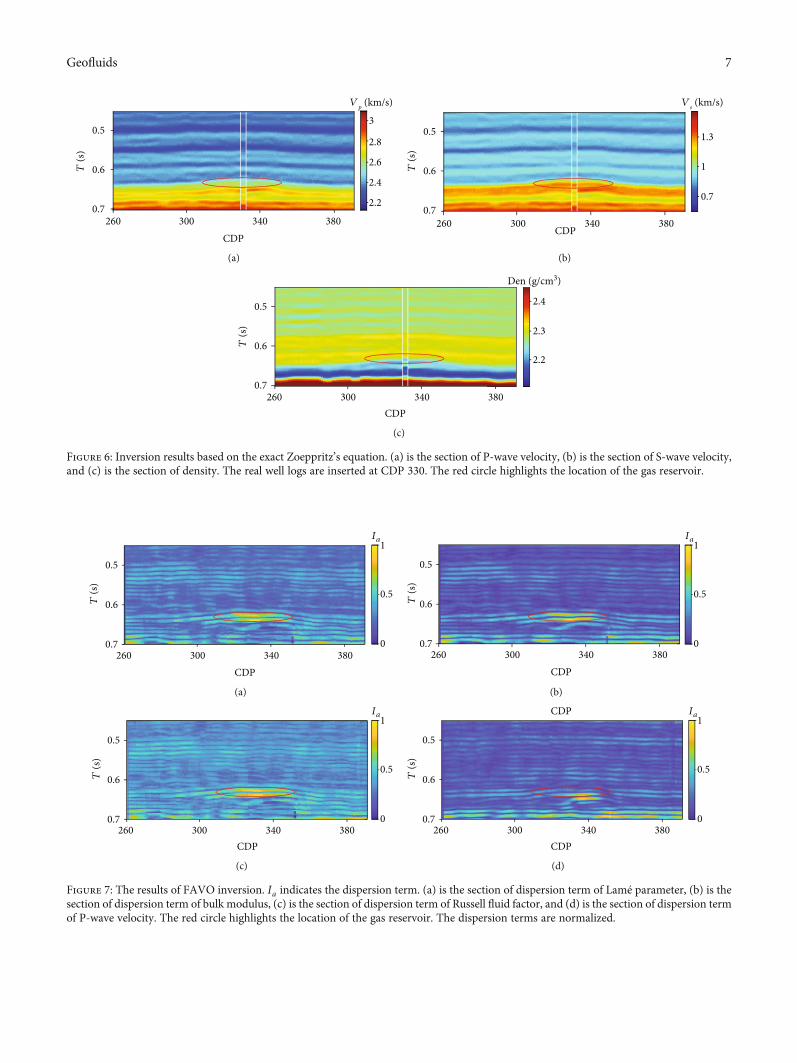
Figure 6: Inversion results based on the exact Zoeppritz’s equation. (a) is the section of P-wave velocity, (b) is the section of S-wave velocity,and (c) is the section of density. The real well logs are inserted at CDP 330. The red circle highlights the location of the gas reservoir.

260 300 340 380CDP

0.5

0.6

0.7

T (s

)

0

0.5

1Ia

(a)

260 300 340 380CDP

0.5

0.6

0.7

T (s

)

0

0.5

1Ia

(b)

260 300 340 380CDP

0.5

0.6

0.7

T (s

)

0

0.5

1Ia

(c)

CDP

260 300 340 380CDP

0.5

0.6

0.7

T (s

)

0

0.5

1Ia

(d)

Figure 7: The results of FAVO inversion. Ia indicates the dispersion term. (a) is the section of dispersion term of Lamé parameter, (b) is thesection of dispersion term of bulk modulus, (c) is the section of dispersion term of Russell fluid factor, and (d) is the section of dispersion termof P-wave velocity. The red circle highlights the location of the gas reservoir. The dispersion terms are normalized.

7Geofluids

where n is the number of angle gathers and m is the numberof frequencies after the spectral decomposition.

3. Application

The used field seismic data set is from HampsonRussell soft-ware, recorded over the shallow Cretaceous. Figure 5 showsthe stack section with gathers from CDP 260 to 390. Theangles vary from 3° to 24°. The dominant frequency is about35Hz. The red circle in Figure 5 indicates the location of gasreservoir with the strong reflector. A real gas well is located atCDP 330. From the well logging data, the lithology of the tar-get reservoir is gas-bearing sandstone and the gas saturationis about 50%. This is a typical gas reservoir, which can beused to test whether our method is valid or not. This set ofdata has been used as an application study by otherresearchers [54].

In order to obtain ðVS/VPÞ2sat in the FAVO inversion, theP- and S-wave velocities are estimated based on the exactZoeppritz’s equation. The Bayesian framework is used toimprove the stability of the inversion. For simplicity,ðVS/VPÞ2sat can be approximated to a fixed value with someaccuracy loss. Figure 6 shows the inversion results. It showsthat the accuracy of P-wave velocity around the red circle issuppressed due to the existence of the gas reservoir comparedwith the overlying strata. Figure 7(d) shows relatively weakerdispersion of P-wave velocity in the gas reservoir. There isalso a deviation in the position of the strong dispersion whichcannot match the reservoir location very well. Figures 7(a)–7(c) (γ2dry = 2:3) have the same dispersion characteristicsand can better identify the fluid. The dispersion ofFigure 7(b) is slightly weaker than that of Figures 7(a) and7(c). Figure 7 shows that the dispersion terms related to Rus-sell fluid factor, Lamé parameter, and bulk modulus are supe-rior to that of P-wave velocity, and among them, Russell fluidfactor is slightly more prominent, followed by Laméparameter.

The value of γ2dry is determined from the well logging

data. Figure 8 shows that all values of ðVP/VSÞ2sat are largerthan 2.3. If we let γ2dry = 4:1 or 8.9, the dispersion term of Rus-sell fluid factor is unsatisfactory (Figures 9(a) and 9(b)).These two values of γ2dry are within the range of ðVP/VSÞ2sat,and they can cause big deviations to the dispersion term.According to the previous analysis, the AVO approximationis accurate when the value of γ2dry is much larger than

ðVP/VSÞ2sat. However, this does not mean that the dispersionterm is correct. Figure 9(c) shows poor dispersion term evenfor a large value of γ2dry (γ

2dry = 15). Therefore, γ2dry should be

smaller than any possibility of ðVP/VSÞ2sat. In addition, fromequations (2), if the value of γ2dry is 2, 4/3, or 0, Russell fluidfactor f can be changed into Lamé parameter λ, bulk modu-lus K , or P-wave modulusM. As depicted in Figure 2, with alarger value of γ2dry, the Russell fluid factor can have moreattenuation induced by the pore fluid.

According to Chen et al. [43], we can derive new P-wavedifference dispersion factor (PDDF) combining with the

P-wave difference. The new PDDFs are related to Russellfluid factor, Lamé parameter, and bulk modulus byreplacing Ia in the following equation:

PDDF = ΔVP ⋅ Ia, ð13Þ

where ΔVP is obtained by subtracting the P-wave velocityof the upper layer from that of the lower layer. Figure 10shows the prediction process of dispersion term and P-wave difference dispersion factor.

Figure 11 indicates that the PDDF is superior to disper-sion term Ia (Figure 7) in fluid discrimination. The sectionof PDDF has better accuracy and better continuity. Due tothe difference in dispersion terms, the PDDF results are dif-ferent obviously. The PDDFs related to Russell fluid factor,Lamé parameter, and bulk modulus are almost similar, andthey are all better than that of P-wave velocity in identifyingthe gas-bearing rocks. By comparison, Russell fluid factor isslightly more obvious.

The various parameter curves at borehole-side trace aredisplayed in Figure 12. In Figure 12, there are two peaks onthe curves of dispersion term and PDDF at the location ofgas reservoir. It is consistent with the analysis of Hampson-Russell software about the two sets of gas layer: top gas andbase gas. The dispersion terms and PDDFs related to Russellfluid factor (f ), Lamé parameter (λ), and bulk modulus (K)are more pronounced. Due to the attenuation and dispersioncaused by the gas reservoir, the inverted P-wave velocity(Figure 12(b)) based on the elastic theory of Zoeppritz’s

2.5 3Vp (km/s)

0.5

0.6

0.7T

(s)

1 1.5Vs (km/s)

0 105(Vp/Vs)2

2.3

(a) (b) (c)

Figure 8: Well logging curves. (a) indicates P-wave velocity; (b)indicates S-wave velocity; (c) indicates ðVP/VSÞ2sat.

8 Geofluids

equation is affected and the prediction accuracy of the lowerlayer is unsatisfactory. This also explains why FAVO inver-sion can be used to identify oil and gas.

4. Discussion and Conclusions

Pore fluid can cause dispersion and attenuation of elasticparameters in the seismic frequency range. Therefore, thestudy of dispersion term of elastic parameter can be bene-ficial for fluid discrimination. By analysis, the shear mod-ulus is almost unaffected by the pore fluid; however, thedispersion and attenuation of Russell fluid factor, Laméparameter, and bulk modulus are stronger and decreasein turn. Uniform expression of dispersion terms of theseparameters is derived, and P-wave difference dispersionfactors are studied by incorporating with P-wavedifference.

The applicability of Russell AVO approximation is ana-lyzed, and an inappropriate weighting parameter associatedwith the dry rock can cause a large deviation. In order toensure that the AVO attribute and the dispersion term arecorrect and reasonable, the value γ2dry should be smaller than

any possibility of ðVP/VSÞ2sat from the well logging data or thelaboratory measurement.

Field data application shows that the dispersion termsrelated to Russell fluid factor with proper weighting parame-ter, Lamé parameter, and bulk modulus are preferable, andamong them, Russell fluid factor is slightly more prominent,followed by Lamé parameter, which is consistent with theChapman model. The P-wave difference dispersion factorsrelated to Russell fluid factor, Lamé parameter, and bulkmodulus are almost similar and better than those of P-wavevelocity, and Russell fluid factor has a slight advantage inidentifying pore fluid.

0.5

0.6

0.7

T (s

)

260 300 340 380CDP

0

0.5

1Ia

(a)

0.5

0.6

0.7

T (s

)

260 300 340 380CDP

0

0.5

1Ia

(b)

260 300 340 380CDP

0.5

0.6

0.7

T (s

)

0

0.5

1Ia

(c)

Figure 9: Analysis of dispersion terms of Russell fluid factor with different γ2dry . (a) corresponds to the dispersion term with γ2dry = 4:1; (b)corresponds to the dispersion term with γ2dry = 8:9; (c) corresponds to the dispersion term with γ2dry = 15; the red circle highlights the

location of the gas reservoir.

Sparse constrained inversionspectral decomposition

Seismic data D(t,𝜃)

Time-frequencyspectrum S(t,𝜃,𝜔)

Time-frequencyspectrum BR(t,𝜃,𝜔)

Spectral balancing

Dispersion term Ia

FAVO inversion

P-wave differencedispersion factor PDDF

P-wave difference

Figure 10: The prediction process of dispersion term and P-wavedifference dispersion factor.

9Geofluids

260 300 340 380CDP

0.5

0.6

0.7

T (s

)

0

0.5

1PDDF

(a)

260 300 340 380CDP

0.5

0.6

0.7

T (s

)

0

0.5

1PDDF

(b)

260 300 340 380CDP

0.5

0.6

0.7

T (s

)

0

0.5

1PDDF

(c)

0

0.5

1PDDF

260 300 340 380CDP

0.5

0.6

0.7

T (s

)

(d)

Figure 11: The P-wave difference dispersion factors of different dispersion terms. PDDF indicates the P-wave difference dispersion factor; (a)is the section of PDDF related to Lamé parameter, (b) is the section of PDDF related to bulk modulus, (c) is the section of PDDF related toRussell fluid factor (γ2dry = 2:3), and (d) is the section of PDDF related to P-wave velocity. The red circle highlights the location of the gas

reservoir. The PDDFs are normalized.

–2 0 2

Trace⨯104

Vp (km/s)

0.5

0.6

0.7

T (s

)

2.5 3 0 0.5 1

Ia

0 0.5 1

Ia

0 0.5 1

Ia

0.4 0.6

Ia

0 0.5

PDDF

0 0.5

PDDF

0 0.5

PDDF

0.4 0.6

PDDF

(i)(f) (g) (h)(e)(d)(c)(b)(a) (j)

K𝜆 𝜆f K f Vp

Vp

Well dataInversion

Figure 12: Display of various parameters at the well location. (a) is the poststack seismic trace; (b) is the P-wave velocity, the red curve is thereal well log after smoothing, and the blue curve is the inverted result; (c) is the dispersion term of Lamé parameter (λ); (d) is the dispersionterm of bulk modulus (K); (e) is the dispersion term of Russell fluid factor (f ) (γ2dry = 2:3); (f) is the dispersion term of P-wave velocity (VP);

(g) is the PDDF of Lamé parameter (λ); (h) is the PDDF of bulk modulus (K); (i) is the PDDF of Russell fluid factor (f ) (γ2dry = 2:3); (j) is thePDDF of P-wave velocity (VP). The yellow dotted rectangle highlights the location of the gas reservoir.

10 Geofluids

Appendix

The Relationship of Some Approximations ofZoeppritz’s Equation

Aki and Richards [27] derived a simplified form of P-wavereflectivity in terms of density and P- and S-wave velocitiesas follows:

RPP θð Þ = 12 sec2θΔVP

VP− 4 sin2θ VS

VP

� �2 ΔVS

VS

+ 12 1 − 4 sin2θ VS

VP

� �2 !

Δρ

ρ,

ðA:1Þ

where θ is the incident angle; VP, VS, and ρ are the P-wavevelocity, S-wave velocity, and density of the fluid-filled rock,respectively; ΔVP/VP, ΔVS/VS, and Δρ/ρ are the P-wavevelocity reflectivity, S-wave velocity reflectivity, and densityreflectivity, respectively; ΔVP , ΔVS, and Δρ are the differ-ences between the lower and upper layers of the interface.

With the relationships between material properties [55],

ΔVP

VP= 12

ΔMM

−Δρ

ρ

� �,

ΔVS

VS= 12

Δμ

μ−Δρ

ρ

� �,

ðA:2Þ

and the relationships between P-wave modulus, S-wavemodulus, bulk modulus, and Lamé parameter summarizedas follows,

ΔM = ΔK + 43Δμ = Δλ + 2Δμ, ðA:3Þ

another two approximation equations can be derived as fol-lows, which are the same as the equations given by Grayet al. [51]:

RPP θð Þ = 14 −

12

VS

VP

� �2

sat

!sec2θ Δλ

λ

+ 12 sec2θ − 2 sin2θ� �

VS

VP

� �2

sat

Δμ

μ

+ 14 1 − tan2θ� �Δρ

ρ,

ðA:4Þ

RPP θð Þ = 14 −

13

VS

VP

� �2

sat

!sec2θ ΔK

K

+ 13 sec2θ − 2 sin2θ� �

VS

VP

� �2

sat

Δμ

μ

+ 14 1 − tan2θ� �Δρ

ρ,

ðA:5Þ

where ΔM/M, Δλ/λ, ΔK/K , and Δμ/μ are the P-wave modu-lus reflectivity, Lamé parameter reflectivity, bulk modulus

reflectivity, and shear modulus reflectivity, respectively; sub-script sat indicates the fluid-filled rock.

Russell et al. [35] derived a new AVO approximation,which has the same form as equations (A.4) and (A.5):

RPP θð Þ = 14 −

γ2dry4

VS

VP

� �2

sat

!sec2θ Δf

f

+γ2dry4 sec2θ − 2 sin2θ

!VS

VP

� �2

sat

Δμ

μ

+ 14 1 − tan2θ� �Δρ

ρ:

ðA:6Þ

If the value of γ2dry is 2 or 4/3, equation (A.6) can reduce

to equation (A.4) or (A.5). Besides, if the value of γ2dry is 0,equation (A.1) can be obtained by multiplying equation(A.6) by 2.

Data Availability

All model data during this study are listed; researchers canreplicate the analysis. But the real seismic data in the applica-tion section are not available because they involve businesssecrets.

Conflicts of Interest

The authors declare that they have no conflicts of interest.

Acknowledgments

The authors gratefully acknowledge financial supportsfrom the National Natural Science Foundation of China(Nos. 41774131, 41774129, and 41874128), the ScienceFoundation of China University of Petroleum, Beijing(No. 2462018QZDX01), and the Young Elite ScientistsSponsorship Program by CAST (No. 2018QNRC001).

References

[1] G. Mavko, T. Mukerji, and J. Dvorkin, The Rock Physics Hand-book: Tools for Seismic Analysis of Porous Media, Cambridgeuniversity press, 2009.

[2] G. T. Kuster and M. N. Toksöz, “Velocity and attenuation ofseismic waves in two-phase media: part I. Theoretical formula-tions,” Geophysics, vol. 39, no. 5, pp. 587–606, 1974.

[3] T. T. Wu, “The effect of inclusion shape on the elastic moduliof a two-phase material,” International Journal of Solids andStructures, vol. 2, no. 1, pp. 1–8, 1966.

[4] J. G. Berryman, “Single-scattering approximations for coeffi-cients in Biot’s equations of poroelasticity,” The Journal ofthe Acoustical Society of America, vol. 91, no. 2, pp. 551–571,1992.

[5] M. A. Biot, “Theory of propagation of elastic waves in a fluid-saturated porous solid. I. Low‐frequency range,” The Journal ofthe Acoustical Society of America, vol. 28, no. 2, pp. 168–178,1956.

11Geofluids

[6] L. Thomsen, “Biot-consistent elastic moduli of porous rocks:low-frequency limit,” Geophysics, vol. 50, no. 12, pp. 2797–2807, 1985.

[7] Z. Wang and A. Nur, “Elastic wave velocities in porous media:a theoretical recipe,” Seismic and Acoustic Velocities in Reser-voir Rocks, vol. 2, pp. 1–35, 1992.

[8] R. G. Keys and S. Xu, “An approximation for the Xu-Whitevelocity model,” Geophysics, vol. 67, no. 5, pp. 1406–1414,2002.

[9] F. Ruiz and A. Cheng, “A rock physics model for tight gassand,” The Leading Edge, vol. 29, no. 12, pp. 1484–1489, 2010.

[10] W. F. Murphy III, “Effects of partial water saturation on atten-uation in Massilon sandstone and Vycor porous glass,” TheJournal of the Acoustical Society of America, vol. 71, no. 6,pp. 1458–1468, 1982.

[11] W. F. Murphy III, “Acoustic measures of partial gas saturationin tight sandstones,” Journal of Geophysical Research: SolidEarth, vol. 89, no. B13, pp. 11549–11559, 1984.

[12] S. Nakagawa, T. J. Kneafsey, T. M. Daley, B. M. Freifeld, andE. V. Rees, “Laboratory seismic monitoring of supercriticalCO2 flooding in sandstone cores using the Split HopkinsonResonant Bar technique with concurrent X-ray computedtomography imaging,” Geophysical Prospecting, vol. 61, no. 2,pp. 254–269, 2013.

[13] J. E. White, “Computed seismic speeds and attenuation inrocks with partial gas saturation,” Geophysics, vol. 40, no. 2,pp. 224–232, 1975.

[14] N. C. Dutta and H. Odé, “Attenuation and dispersion of com-pressional waves in fluid-filled porous rocks with partial gassaturation (White model)-part I: Biot theory,” Geophysics,vol. 44, no. 11, pp. 1777–1788, 1979.

[15] D. L. Johnson, “Theory of frequency dependent acoustics inpatchy-saturated porous media,” The Journal of the AcousticalSociety of America, vol. 110, no. 2, pp. 682–694, 2001.

[16] M. Chapman, S. V. Zatsepin, and S. Crampin, “Derivation of amicrostructural poroelastic model,” Geophysical Journal Inter-national, vol. 151, no. 2, pp. 427–451, 2002.

[17] M. Chapman, “Frequency-dependent anisotropy due to meso-scale fractures in the presence of equant porosity,” GeophysicalProspecting, vol. 51, no. 5, pp. 369–379, 2003.

[18] X. Wu, M. Chapman, X. Y. Li, and P. Boston, “Quantitative gassaturation estimation by frequency-dependent amplitude-versus-offset analysis,” Geophysical Prospecting, vol. 62, no. 6,pp. 1224–1237, 2014.

[19] J. G. Berryman and H. F. Wang, “Elastic wave propagation andattenuation in a double-porosity dual- permeability medium,”International Journal of Rock Mechanics and Mining Sciences,vol. 37, no. 1-2, pp. 63–78, 2000.

[20] V. Grechka, P. Mazumdar, and S. A. Shapiro, “Predicting per-meability and gas production of hydraulically fractured tightsands from microseismic data,” Geophysics, vol. 75, no. 1,pp. B1–B10, 2010.

[21] C. Ecker, J. Dvorkin, and A. Nur, “Sediments with gashydrates: internal structure from seismic AVO,” Geophysics,vol. 63, no. 5, pp. 1659–1669, 1998.

[22] A. Buland and H. Omre, “Bayesian linearized AVO inversion,”Geophysics, vol. 68, no. 1, pp. 185–198, 2003.

[23] X. Pan, G. Zhang, and X. Yin, “Elastic impedance variationwith angle and azimuth inversion for brittleness and fractureparameters in anisotropic elastic media,” Surveys in Geophys-ics, vol. 39, no. 5, pp. 965–992, 2018.

[24] L. Zhou, J. Li, X. Chen, X. Liu, and L. Chen, “Prestack ampli-tude versus angle inversion for Young’s modulus and Poisson’sratio based on the exact Zoeppritz equations,” GeophysicalProspecting, vol. 65, no. 6, pp. 1462–1476, 2017.

[25] W. Alemie and M. D. Sacchi, “High-resolution three-termAVO inversion by means of a Trivariate Cauchy probabilitydistribution,” Geophysics, vol. 76, no. 3, pp. R43–R55, 2011.

[26] R. Gehrmann, C. Müller, P. Schikowsky, T. Henke,M. Schnabel, and C. Bönnemann, “Model-based identificationof the base of the gas hydrate stability zone in multichannelreflection seismic data, Offshore Costa Rica,” InternationalJournal of Geophysics, vol. 2009, Article ID 812713, 12 pages,2009.

[27] K. Aki and P. G. Richards, Quantitative Seismology: Theoryand Methods, University Science Books, San Francisco, 1980.

[28] R. T. Shuey, “A simplification of the Zoeppritz equations,”Geophysics, vol. 50, no. 4, pp. 609–614, 1985.

[29] G. C. Smith and P. M. Gidlow, “Weighted stacking for rockproperty estimation and detection of gas,” Geophysical Pro-specting, vol. 35, no. 9, pp. 993–1014, 1987.

[30] J. L. Fatti, G. C. Smith, P. J. Vail, P. J. Strauss, and P. R. Levitt,“Detection of gas in sandstone reservoirs using AVO analysis:a 3-D seismic case history using the Geostack technique,” Geo-physics, vol. 59, no. 9, pp. 1362–1376, 1994.

[31] L. Zhi, S. Chen, and X. Li, “Amplitude variation with angleinversion using the exact Zoeppritz equations—theory andmethodology,” Geophysics, vol. 81, no. 2, pp. N1–N15, 2016.

[32] Z. Zong, X. Yin, and G. Wu, “Geofluid discriminationincorporating poroelasticity and seismic reflection inver-sion,” Surveys in Geophysics, vol. 36, no. 5, article 9330,pp. 659–681, 2015.

[33] D. Grana, T. Fjeldstad, and H. Omre, “Bayesian Gaussian mix-ture linear inversion for geophysical inverse problems,”Math-ematical Geosciences, vol. 49, no. 4, pp. 493–515, 2017.

[34] B. Goodway, T. Chen, and J. Downton, “Improved AVO fluiddetection and lithology discrimination using Lamé petrophysi-cal parameters; “λρ”, “μρ”, & “λ/μ fluid stack”, from P and Sinversions,” in SEG Technical Program Expanded Abstracts1997, pp. 183–186, Society of Exploration Geophysicists, 1997.

[35] B. H. Russell, D. Gray, and D. P. Hampson, “Linearized AVOand poroelasticity,” Geophysics, vol. 76, no. 3, pp. C19–C29,2011.

[36] B. H. Russell, K. Hedlin, F. J. Hilterman, and L. R. Lines,“Fluid-property discrimination with AVO: a Biot-Gassmannperspective,” Geophysics, vol. 68, no. 1, pp. 29–39, 2003.

[37] A. Alshangiti, “Frequency-dependent AVO inversion: com-parison of different AVO approximations,” in SEG TechnicalProgram Expanded Abstracts 2019, pp. 724–728, Society ofExploration Geophysicists, 2019.

[38] A. Wilson, M. Chapman, and X. Y. Li, “Frequency-dependentAVO inversion,” in SEG Technical Program ExpandedAbstracts 2009, pp. 341–345, Society of Exploration Geophys-icists, 2009.

[39] X. Wu, M. Chapman, A. Wilson, and X.-Y. Li, “Estimatingseismic dispersion from pre-stack data using frequency-dependent AVO inversion,” in SEG Technical ProgramExpanded Abstracts 2010, pp. 425–429, Society of ExplorationGeophysicists, 2010.

[40] C. Luo, G. Huang, and X. Li, “Frequency-dependent AVOinversion based on sparse constrained inversion spectraldecomposition,” in SEG Technical Program Expanded

12 Geofluids

Abstracts 2017, pp. 524–528, Society of Exploration Geophys-icists, 2017.

[41] J. Liu, J. Ning, X. Liu, C. Y. Liu, and T. S. Chen, “An improvedscheme of frequency-dependent AVO inversion method andits application for tight gas reservoirs,” Geofluids, vol. 2019,Article ID 3525818, 12 pages, 2019.

[42] Z. Zhang, X. Y. Yin, and Z. Y. Zong, “A new frequency-dependent AVO attribute and its application in fluid identifi-cation,” in 75th EAGE Conference & Exhibition incorporatingSPE EUROPEC 2013, European Association of Geoscientists& Engineers, June 2013.

[43] R. Chen, X. Chen, J. Li, Z. Wang, and B. Wang, “A new hydro-carbon indicator derived from FAVO inversion,” in SEG Tech-nical Program Expanded Abstracts 2016, pp. 516–520, Societyof Exploration Geophysicists, 2016.

[44] K. Wang, X. Chen, D. Wang et al., “A new insight into thehydrocarbon indicator of tight sandstone reservoir,” in SEGTechnical Program Expanded Abstracts 2018, pp. 401–405,Society of Exploration Geophysicists, 2018.

[45] Y. Wang, X. Ma, H. Zhou, and Y. Chen, “L1− 2 minimizationfor exact and stable seismic attenuation compensation,” Geo-physical Journal International, vol. 213, no. 3, pp. 1629–1646,2018.

[46] M. Chapman, E. Liu, and X. Y. Li, “The influence of fluid-sensitive dispersion and attenuation on AVO analysis,” Geo-physical Journal International, vol. 167, no. 1, pp. 89–105,2006.

[47] E. Fjar, R. M. Holt, A. M. Raaen, R. Risnes, and P. Horsrud,Petroleum Related Rock Mechanics, Elsevier, 2008.

[48] D. C. Bonar and M. D. Sacchi, “Complex spectral decomposi-tion via inversion strategies,” in SEG Technical ProgramExpanded Abstracts 2010, pp. 1408–1412, Society of Explora-tion Geophysicists, 2010.

[49] S. Yuan, Z. Yu, H. Gao et al., “Semi-blind time-variant sparsedeconvolution using a weighted L1 norm,” in 81st EAGE Con-ference and Exhibition 2019, European Association of Geosci-entists & Engineers, June 2019.

[50] E. Van Den Berg and M. P. Friedlander, “Probing the Paretofrontier for basis pursuit solutions,” SIAM Journal on ScientificComputing, vol. 31, no. 2, pp. 890–912, 2009.

[51] D. Gray, B. Goodway, and T. Chen, “Bridging the gap: usingAVO to detect changes in fundamental elastic constants,” inSEG Technical Program Expanded Abstracts 1999, pp. 852–855, Society of Exploration Geophysicists, 1999.

[52] G. Partyka, J. Gridley, and J. Lopez, “Interpretational applica-tions of spectral decomposition in reservoir characterization,”The Leading Edge, vol. 18, no. 3, pp. 353–360, 1999.

[53] E. Odebeatu, J. Zhang, M. Chapman, E. Liu, and X. Y. Li,“Application of spectral decomposition to detection of disper-sion anomalies associated with gas saturation,” The LeadingEdge, vol. 25, no. 2, pp. 206–210, 2006.

[54] H. Liu, J. Li, X. Chen, B. Hou, and L. Chen, “Amplitude varia-tion with offset inversion using the reflectivity method,” Geo-physics, vol. 81, no. 4, pp. R185–R195, 2016.

[55] Z. Zong, X. Yin, and G. Wu, “AVO inversion and poroelasti-city with P-and S-wave moduli,” Geophysics, vol. 77, no. 6,pp. N17–N24, 2012.

13Geofluids

Hindawiwww.hindawi.com Volume 2018

Journal of

ChemistryArchaeaHindawiwww.hindawi.com Volume 2018

Marine BiologyJournal of

Hindawiwww.hindawi.com Volume 2018

BiodiversityInternational Journal of

Hindawiwww.hindawi.com Volume 2018

EcologyInternational Journal of

Hindawiwww.hindawi.com Volume 2018

Hindawiwww.hindawi.com

Applied &EnvironmentalSoil Science

Volume 2018

Forestry ResearchInternational Journal of

Hindawiwww.hindawi.com Volume 2018

Hindawiwww.hindawi.com Volume 2018

International Journal of

Geophysics

Environmental and Public Health

Journal of

Hindawiwww.hindawi.com Volume 2018

Hindawiwww.hindawi.com Volume 2018

International Journal of

Microbiology

Hindawiwww.hindawi.com Volume 2018

Public Health Advances in

AgricultureAdvances in

Hindawiwww.hindawi.com Volume 2018

Agronomy

Hindawiwww.hindawi.com Volume 2018

International Journal of

Hindawiwww.hindawi.com Volume 2018

MeteorologyAdvances in

Hindawi Publishing Corporation http://www.hindawi.com Volume 2013Hindawiwww.hindawi.com

The Scientific World Journal

Volume 2018Hindawiwww.hindawi.com Volume 2018

ChemistryAdvances in

Scienti�caHindawiwww.hindawi.com Volume 2018

Hindawiwww.hindawi.com Volume 2018

Geological ResearchJournal of

Analytical ChemistryInternational Journal of

Hindawiwww.hindawi.com Volume 2018

Submit your manuscripts atwww.hindawi.com