unsteady fluid mechanics of starting-flow...
TRANSCRIPT

UNSTEADY FLUID MECHANICS OF STARTING-FLOW VORTEX GENERATORS WITH
TIME-DEPENDENT BOUNDARY CONDITIONS
Thesis by
John Oluseun Dabiri
In Partial Fulfillment of the Requirements for the Degree of
Doctor of Philosophy
CALIFORNIA INSTITUTE OF TECHNOLOGY
Pasadena, California
2005
(Defended April 8, 2005)

ii
2005
John Oluseun Dabiri
All Rights Reserved

iii
Acknowledgements
Above all else, I thank my Lord and Savior Jesus Christ for His grace, strength,
guidance, and wisdom as I have pursued a fuller understanding of his Creation. Let this
thesis stand as a testament of His abundant love for each of us.
I have been crucified with Christ; it is no longer I who live, but Christ lives in me; and the life which I now live in the flesh I live by faith in the Son of God, who loved me and gave Himself for me. --Galatians 2:20
My family has provided continual support and encouragement since I first realized
a passion for learning as a child. It is their care, along with the love and patience of Melissa
Suzanne Blue, which has motivated me during difficult times.
My thesis advisor Mory Gharib has imbued in me the art of scientific investigation.
It is under his tutelage that I have gained the perspective to approach classical problems in
science and the confidence to solve new ones.
I have benefited from the advice, collaboration, and companionship of a host of
memorable individuals associated with science education, including Messrs. David
Barrows and Robert Shawver; Mrs. JoAnn Love; Drs. Edgar Choueiri, Michael Littman,
Alexander Smits, Boguslaw Gajdeczko, Philip Felton, Frederick Dryer, Luigi Martinelli,
Jay Hove, Michele Milano, Nikoo Saber, David Jeon, Paul Krueger, John Costello, Sean
Colin, Tait Pottebaum, Matthew Ringuette, Gabriel Acevedo-Bolton, and Arash
Kheradvar; Mmes. Kathleen Hamilton and Martha Salcedo; Mmes. Anna Hickerson and
Rebecca Rakow-Penner; and Messrs. Arian Forouhar, Lance Cai, Ben Lin, Emilio Graff,
and Derek Rinderknecht. I am especially grateful for the generous comments of Profs. John
Brady, Joel Burdick, Michael Dickinson, Anthony Leonard, and Dale Pullin on this work.

iv
Abstract
Nature has repeatedly converged on the use of starting flows for mass, momentum,
and energy transport. The vortex loops that form during flow initiation have been
reproduced in the laboratory and have been shown to make a proportionally larger
contribution to fluid transport than an equivalent steady jet. However, physical processes
limit growth of the vortex loops, suggesting that these flows may be amenable to
optimization. Although it has been speculated that optimal vortex formation might occur
naturally in biological systems, previous efforts to quantify the biological mechanisms of
vortex formation have been inconclusive. In addition, the unsteady fluid dynamical effects
associated with starting flow vortex generators are poorly understood.
This thesis describes a combination of new experimental techniques and in vivo
animal measurements that determine the effects of fluid-structure interactions on vortex
formation by starting flow propulsors. Results indicate that vortex formation across
various biological systems is manipulated by these kinematics in order to maximize thrust
and/or propulsive efficiency. An emphasis on observed vortex dynamics and transient
boundary conditions facilitates quantitative comparisons across fluid transport schemes,
irrespective of their individual biological functions and physical scales.
The primary contributions of this thesis are the achievement of quantitative
measures of unsteady vortex dynamics via fluid entrainment and added-mass effects, and
the development of a robust framework to facilitate the discovery of general design
principles for effective fluid transport in engineering technologies and biological therapies.
The utility of this new research paradigm is demonstrated through a variety of examples.

v
Table of Contents
Acknowledgements .................................................................................................................iii
Abstract ....................................................................................................................................iv
Table of Contents......................................................................................................................v
List of Figures ........................................................................................................................viii
CHAPTER 1: Prologue ...........................................................................................................1
CHAPTER 2: Fluid entrainment by isolated vortex rings......................................................4 2.0 Chapter Abstract..........................................................................................................4 2.1 Introduction .................................................................................................................5 2.2 Measurement Techniques ...........................................................................................9
2.2.1 Apparatus............................................................................................................9 2.2.2 Counter-flow protocols .....................................................................................11
2.3 Results........................................................................................................................13 2.3.1 Vortex ring trajectories ....................................................................................13 2.3.2 Fluid entrainment and vorticity distribution....................................................15
2.4 Comparison with Maxworthy (1972) .......................................................................24 2.5 A Quantitative Model for Diffusive Fluid Entrainment...........................................31 2.6 Conclusions ...............................................................................................................35 2.7 Chapter References....................................................................................................38
CHAPTER 3: A contribution from wake vortex added-mass in estimates of animal swimming and flying dynamics.....................................................................41
3.0 Chapter Abstract........................................................................................................41 3.1 Introduction ...............................................................................................................41 3.2 Methods .....................................................................................................................44 3.3 Results........................................................................................................................45 3.4 Discussion..................................................................................................................52 3.5 Chapter References....................................................................................................54
CHAPTER 4: Delay of vortex ring pinch-off by an imposed bulk counter-flow ...............57 4.0 Chapter Abstract........................................................................................................57 4.1 Introduction ...............................................................................................................57 4.2 Methods and Results .................................................................................................59 4.3 Conclusions ...............................................................................................................64 4.4 Chapter References....................................................................................................65
CHAPTER 5: A revised slug model boundary layer correction for starting jet vorticity flux..................................................................................................................67
5.0 Chapter Abstract........................................................................................................67 5.1 Introduction ...............................................................................................................67 5.2 Revised Correction....................................................................................................69

vi 5.3 Conclusions ...............................................................................................................71 5.4 Chapter References....................................................................................................71
CHAPTER 6: Starting flow through nozzles with temporally variable exit diameter ........73 6.0 Chapter Abstract........................................................................................................73 6.1 Introduction ...............................................................................................................74 6.2 Apparatus and Experimental Methods......................................................................79
6.2.1 Apparatus design..............................................................................................79 6.2.2 Effects of noncircular nozzle shape.................................................................84 6.2.3 Quantitative flow visualization........................................................................85 6.2.4 Experimental parameter space.........................................................................86 6.2.5 Boundary layer dynamics ................................................................................88
6.3 Results........................................................................................................................92 6.3.1 Vorticity flux ....................................................................................................92 6.3.2 Dimensional analysis .......................................................................................95 6.3.3 Leading vortex ring pinch-off and vorticity distribution ................................98 6.3.4 Leading vortex ring energy............................................................................103 6.3.5 Leading vortex ring fluid transport................................................................109
6.4 Summary and Conclusions......................................................................................111 6.5 Chapter References..................................................................................................115
CHAPTER 7: Sensitivity analysis of kinematic approximations in dynamic medusan swimming models ........................................................................................120
7.0 Chapter Abstract......................................................................................................120 7.1 Introduction .............................................................................................................120 7.2 Materials and Methods............................................................................................122
7.2.1 Video recording and image processing .........................................................122 7.2.2 Dynamical model ...........................................................................................124 7.2.3 Sensitivity analysis—bell volume and aperture area ....................................125 7.2.4 Sensitivity analysis—fineness ratio...............................................................126
7.3 Results......................................................................................................................128 7.3.1 Bell volume and aperture area approximations.............................................128 7.3.2 Fineness ratio approximation.........................................................................128
7.4 Discussion................................................................................................................131 7.5 Chapter References..................................................................................................135
CHAPTER 8: The role of optimal vortex formation in biological fluid transport ............137 8.0 Chapter Abstract......................................................................................................137 8.1 Introduction .............................................................................................................138 8.2 Methods ...................................................................................................................140
8.2.1 Kinematic analysis .........................................................................................140 8.2.2 Laboratory apparatus......................................................................................141
8.3 Results......................................................................................................................141 8.3.1 Laboratory results...........................................................................................141 8.3.2 Biological optimization strategy....................................................................143

vii 8.3.3 Comparison with in situ squid measurements...............................................144 8.3.4 Comparison with in vivo cardiac measurements ..........................................145
8.4 Discussion................................................................................................................147 8.5 Chapter References..................................................................................................148
CHAPTER 9: Flow patterns generated by oblate medusan jellyfish: field measurements and laboratory analyses................................................................................151
9.0 Chapter Abstract......................................................................................................151 9.1 Introduction .............................................................................................................152 9.2 Methods ...................................................................................................................155
9.2.1 Video measurements......................................................................................155 9.2.2 Kinematic analyses ........................................................................................156 9.2.3 Strategies for dye marker interpretation ........................................................157
9.3 Results......................................................................................................................158 9.3.1 Vortex formation process...............................................................................158 9.3.2 Tentacle positioning.......................................................................................163 9.3.3 Vortex ring kinematic measurements............................................................164
9.4 Discussion................................................................................................................166 9.4.1 Implications for medusan swimming behavior .............................................166 9.4.2 Implications for medusan feeding behavior ..................................................170 9.4.3 Implications for prolate medusae...................................................................171 9.4.4 A note on fluid dynamic and geometric scaling............................................174
9.5 Chapter References..................................................................................................175

viii
List of Figures
Figure 2.1 Schematic of apparatus for piston-cylinder experiments....................................10 Figure 2.2 Measured vortex ring trajectory for each counter-flow protocol .......................14 Figure 2.3 Instantaneous streamlines for protocol LD2-CF0 at time T = 5.34 s .................16 Figure 2.4 Measured entrainment fraction η(t) for each counter-flow protocol ..................18 Figure 2.5 Instantaneous streamlines and vorticity patches for protocol LD2-CF0............21 Figure 2.6 Measured vortex ring core vorticity profiles.......................................................22 Figure 2.7 Measured vortex ring velocity for each counter-flow protocol..........................25 Figure 2.8 Measured vortex ring circulation for each counter-flow protocol......................28 Figure 2.9 Instantaneous streamlines and vorticity patches for protocol LD2-CF0............30 Figure 2.10 Comparison of predicted vortex growth to experimental measurements.........35 Figure 3.1 DPIV measurements of free-swimming jellyfish and a mechanical analogue ..46 Figure 3.2 Demonstration of heuristic (i.e., Darwin, 1953) for measuring solid body added-
mass................................................................................................................49 Figure 3.3 Measurements of Lagrangian drift induced by translating fluid vortices ..........50 Figure 3.4 Drift and fluid body volume measurements for translating vortices..................51 Figure 4.1 Schematic of basic apparatus for counter-flow experiments..............................60 Figure 4.2 Circulation versus nondimensional time for nominal stroke ratio of 4..............61 Figure 4.3 Nondimensional time versus physical time.........................................................63 Figure 5.1 Comparison of slug models of vorticity flux with DPIV measurements ...........70 Figure 6.1 Apparatus for temporal variation of nozzle exit diameter ..................................83 Figure 6.2 Programs of nozzle exit diameter temporal variation.........................................87 Figure 6.3 Rate of diameter change for each program of nozzle exit diameter temporal
variation..........................................................................................................87 Figure 6.4 Velocity profile of fluid efflux at X = 0.3 Dp for static minimum and maximum
diameter cases ................................................................................................91 Figure 6.5 Measured and predicted circulation generated for each program of nozzle exit
diameter temporal variation...........................................................................94 Figure 6.6 Normalized circulation versus formation time for each program of nozzle exit
diameter temporal variation...........................................................................97 Figure 6.7 Normalized circulation versus formation time for SMIN, SO, and FO cases .100 Figure 6.8 Vorticity profile along radial section of vortex ring core for SMIN, SO, and FO
cases .............................................................................................................100 Figure 6.9 Normalized circulation versus formation time for SMAX, SC, and FC cases 102 Figure 6.10 Vorticity profile along radial section of vortex ring core for SMAX, SC, and
FC cases .......................................................................................................102 Figure 6.11 Normalized vortex generator energy versus formation time ..........................105 Figure 6.12 Vorticity contours of the flow downstream of the static maximum diameter
nozzle ...........................................................................................................107 Figure 6.13 Vorticity contours of the flow downstream of the FC diameter nozzle .........107 Figure 6.14 Delivered fluid fraction for leading vortex rings in nozzle cases with
temporally variable exit diameter................................................................110

ix Figure 7.1 Video recording and image processing .............................................................124 Figure 7.2 Measurements of Chrysaora fuscescens swimming.........................................127 Figure 7.3 Dynamical swimming models for each test case ..............................................129 Figure 7.4 Measured and computed fineness ratio .............................................................130 Figure 7.5 Modeled swimming dynamics from fineness ratio measurement inputs .........130 Figure 7.6 Ratio of diameter for exact fineness-hemiellipsoid model to bell aperture
diameter........................................................................................................133 Figure 8.1 Schematic of jet flow apparatus with time-varying nozzle exit diameter ........142 Figure 8.2 Vorticity profiles for different rates of jet exit diameter temporal increase.....143 Figure 8.3 Tail-first swimming kinematics of Lolliguncula brevis ...................................145 Figure 8.4 Trans-mitral flow during normal and pathological early diastolic filling ........147 Figure 9.1 Schematic of a jetting medusa with vortex rings in the wake ..........................153 Figure 9.2 Video sequence of vortex ring formation during two swimming cycles of
Aurelia aurita...............................................................................................159 Figure 9.3 Kinematics of the starting, stopping, and co-joined lateral vortex structures ..161 Figure 9.4 Video sequence and schematic of fluorescent dye relative to the tentacles of
Aurelia aurita during a swimming cycle ....................................................164 Figure 9.5 Medusa bell shape profiles normalized by volume of ejected bell fluid Ωb ....175

1
CHAPTER 1: Prologue
This thesis is comprised of peer-reviewed articles from archival journals spanning
the experimental and theoretical practices of engineering and biology. The organization is
intentional and meant to underscore the interdisciplinary nature of the topics at hand while
fomenting a clear emphasis on the discipline-specific contributions of this work.
The thesis author is also the lead author of each article and wrote all (Chapters 2
through 8) or the large majority (Chapter 9, all sections save parts of 9.2.1, 9.3.1, and 9.3.2)
of the text in each case.
The articles are arranged with the goal of presenting results related to the physics of
fluids first, followed by directed studies of biological applications. Chapters 2 and 3
investigate the primary unsteady effects in starting flows, namely fluid entrainment and
added-mass dynamics. In both cases, new experimental techniques were developed to
facilitate the first fully quantitative measurements of the associated fluid mechanics and, in
the latter case, to demonstrate the existence of that unsteady component for the first time.
Chapters 4 and 5 examine the role of boundary layer kinematics in dictating the
dynamics of vortex formation and saturation. In the first of these two chapters, a model is
developed to predict the flux of vorticity from a starting jet. Its accuracy is shown to be an
order of magnitude greater than existing standard models. Chapter 5 describes the
development of an experimental method to manipulate shear layer kinematics in order to
achieve the first artificial delay of vortex saturation, a result that has been considered in this
research field a necessary condition for augmentation of starting jet fluid transport.

2 The results of Chapters 4 and 5 are incorporated into Chapter 6, which brings
together boundary layer kinematics, vortex dynamics, and fluid-structure interactions in
experiments aimed at addressing the fluid mechanics of biologically-relevant starting
flows. The results indicate the importance of properly accounting for the time-dependent
boundary conditions that are commonly observed in Nature and suggest that a rich diversity
of fluid dynamical effects can be induced by relatively simple fluid-structure interactions.
This chapter serves a dual role, both as a fundamental investigation of fluid mechanics and
as a robust framework for studies of biological fluid transport systems.
Chapter 7 introduces the first dedicated studies of biological fluid transport in the
thesis, using jellyfish as the model system. Its primary contribution is to highlight
difficulties in modeling swimming dynamics based solely on propulsor morphology and
kinematics. Chapter 8 takes this message further and illustrates the ability of the framework
developed in Chapter 6 to predict normal and pathological function of biological fluid
transport systems, with greater fidelity than is afforded by prevalent methods. Consistent
with the overall theme of this thesis, the role of fluid-structure interactions and their proper
modeling is emphasized. Importantly, it is shown that the principles of optimal vortex
formation apply to a broad range of biological systems and can be analyzed quantitatively
in each case without the need to reference details of their specific biological functionalities.
Finally, Chapter 9 describes the first quantitative, in situ field measurements of
jellyfish swimming and related fluid dynamics. Results indicate that even for the simple
morphology of these animals, the generated flow field can be quite complex. The careful
tuning and coordination of multiple jellyfish functions that is achieved solely by exploiting
fluid dynamics is fascinating, but also hints at the magnitude of our challenge in replicating

3 and improving upon these and other biological systems in engineering contexts. This thesis
is effective if it inspires the reader to accept that challenge and the rewards that will follow.

4
CHAPTER 2: Fluid entrainment by isolated vortex rings
Submitted to Journal of Fluid Mechanics April 15, 2004
2.0 Chapter Abstract
Of particular importance to the development of models for isolated vortex ring
dynamics in a real fluid is knowledge of ambient fluid entrainment by the ring. This time-
dependent process dictates changes in the volume of fluid that must share impulse
delivered by the vortex ring generator. Therefore fluid entrainment is also of immediate
significance to the unsteady forces that arise due to the presence of vortex rings in starting
flows. Applications, ranging from industrial and transportation to animal locomotion and
cardiac flows, are currently being investigated to understand the dynamical role of the
observed vortex ring structures. Despite this growing interest, fully empirical
measurements of fluid entrainment by isolated vortex rings have remained elusive. The
primary difficulties arise in defining the unsteady boundary of the ring, as well as an
inability to maintain the vortex ring in the test section sufficiently long to facilitate
measurements. We present a new technique for entrainment measurement that utilizes a
coaxial counter-flow to retard translation of vortex rings generated from a piston-cylinder
apparatus, so that their growth due to fluid entrainment can be observed. Instantaneous
streamlines of the flow are used to determine the unsteady vortex ring boundary and
compute ambient fluid entrainment. Measurements indicate that the entrainment process
does not promote self-similar vortex ring growth, but instead consists of a rapid
convection-based entrainment phase during ring formation, followed by a slower diffusive
mechanism that entrains ambient fluid into the isolated vortex ring. Entrained fluid

5 typically constitutes 30% to 40% of the total volume of fluid carried with the vortex ring.
Various counter-flow protocols were used to substantially manipulate the diffusive
entrainment process, producing rings with entrained fluid fractions up to 65%.
Measurements of vortex ring growth rate and vorticity distribution during diffusive
entrainment are used to explain those observed effects, and a model is developed to relate
the governing parameters of isolated vortex ring evolution. Measurement results are
compared with previous studies of the process, and implications for the dynamics of
starting flows are suggested.
2.1 Introduction
The earliest theoretical treatments of isolated vortex ring kinematics and dynamics
predate quantitative experimental observations of the same phenomena by a half-century,
due largely to the lack of available techniques to measure the salient fluid mechanics.
Although ideal vortex ring models such as those of Saffman (1970), Fraenkel (1972), and
Norbury (1973) have remained popular for describing empirical vortex ring dynamics (e.g.,
Gharib, Rambod and Shariff, 1998; Linden and Turner, 2001), the past few decades of
research have witnessed several efforts to reconcile the predictions of analytical models
with more recent observations made in the laboratory.
The most common method for generating vortex rings in the laboratory is the
piston-cylinder arrangement. In this configuration, a cylindrical piston with outer diameter
flush to the inner diameter of a hollow cylinder is translated axially from rest. A fluid efflux
emerges after separating from the sharp-edged lip at the open end of the hollow cylinder.

6 The resulting cylindrical vortex sheet induces its own roll-up into a ring, which propagates
axially away from the exit plane of the generator.
Vortex rings generated in the laboratory tend to depart from the thin-ring limit
typically studied in theory. Nevertheless the literature contains notable examples of
agreement between classical theoretical predictions and empirical observations (e.g.,
Widnall and Sullivan, 1973; Liess and Didden, 1976).
Maxworthy (1972) credits Reynolds (1876) with the first qualitatively correct
observations of vortex ring propagation subsequent to the formation process. Specifically,
Reynolds describes the growth of the ring in time due to entrainment of fluid surrounding
the ring. Assuming the ring itself possesses a nominally constant impulse, the ring velocity
decreases as a consequence of shared momentum with an increasing mass of fluid.
A physical mechanism for ambient fluid entrainment consisting of repeated cycles
of viscous diffusion and circulatory transport is proposed by Maxworthy (1972). Vorticity
from the core of the isolated vortex ring diffuses to its radial extent, where it interacts with
oncoming irrotational fluid (in the reference frame of the vortex ring). A process of viscous
dissipation reduces the total pressure of the fluid adjacent to the ring, to the point that it
cannot pass over the ring and is instead entrained by the circulatory motion of the ring. A
portion of the diffused vorticity will return to the ring in this entrainment process, while the
remainder will form a small wake behind the ring. Formation of the wake is facilitated by
free-stream fluid that still possesses sufficient total pressure after the dissipation process to
convect the vorticity downstream.
Using dimensional analysis and physical arguments regarding the structure of the
dissipation region, Maxworthy (1972) derives the rate of fluid entrainment as

7
212321
dd
vB UaC
tν
Ω= , (2.1.1)
where is the volume of the vortex bubble (i.e., the volume of fluid moving with the
ring), ν is the kinematic viscosity, a is a characteristic dimension of the ring, and U
BΩ
v is the
characteristic velocity of the free-stream fluid relative to the ring. The quantity C is a
dimensionless lumped parameter that incorporates the shape and size of the dissipation
region, assuming self-similar vortex bubble growth. Equation (2.1.1) is used in concert
with an assumption of constant vortex ring impulse to predict a -2/3 power-law decay of
ring circulation in time, and to hypothesize the existence of a small wake of vorticity
behind the ring.
Despite this progress, Maxworthy (1972) does not attempt to estimate the
magnitude of the lumped parameter and therefore cannot attain a quantitative result for the
contribution of entrainment to the dynamics of vortex rings. Maxworthy (1972) also lacks a
method to empirically verify the predictions of ring circulation decay and wake formation.
The validity of the assumption of constant ring impulse remains unknown, although
Maxworthy (1972) limits it to high Reynolds numbers and small time scales.
Baird, Wairegi and Loo (1977) briefly address the role of fluid entrainment
quantitatively, using the classical slug model (cf. Shariff and Leonard, 1992) to
approximate the fraction of vortex ring fluid that originated in the free stream. They arrive
at the result that 1/4 of the fluid in the vortex ring is supplied by entrainment. The validity
of the calculation is limited to small piston stroke length-to-diameter ratios—less than 2L/D
by their own assertion—so that it can be assumed that all of the impulse delivered from the

8 vortex generator is transferred to the vortex ring. Confirmation of the prediction is not
reported in those experiments or in subsequent work.
Müller and Didden (1980) visualize the growth of vortex rings using a dye marker
in the flow and estimate the entrained fluid fraction of the vortex ring to be approximately
40%. As this was an estimated average value, no conclusions regarding the temporal
dependence of the process can be made.
Transient measurements of fluid entrainment in vortex rings are especially
cumbersome due to difficulty in observing and defining the boundary of the vortex ring as
it propagates in time. Maxworthy (1972) notes that the physical extent of the ring may not
be accurately determined from common dye visualizations, due to marked differences in
the diffusion coefficients of the vorticity and the dye marker (e.g., Schmidt number ~ 102
for Rhodamine WT). As such, he notes the propensity to misinterpret qualitative
visualizations of the entrainment process (e.g., Prandtl and Tietjens, 1934). Fully
quantitative measurements of unsteady ambient fluid entrainment by isolated vortex rings
have not yet been accomplished.
The task of measuring fluid entrainment is simplified if the ring can be maintained
within the measurement window for longer periods of time. In the absence of external
intervention, the ring will propagate away from the vortex generator under its self-induced
velocity. The time allotted for an entrainment measurement will then be dictated by the
length of the viewing window and the ring speed.
A set of experiments was conducted to demonstrate use of an axisymmetric
counter-flow to maintain the vortex ring within the measurement window for longer
periods of time, with the goal of observing ring growth due to fluid entrainment.
9 Instantaneous streamlines of the flow in the reference frame of the vortex ring were
measured using quantitative flow visualization techniques. These data enabled definition of
the unsteady boundary of the vortex ring for transient entrainment calculations.
Although convective transport dominates the fluid entrainment process during
vortex ring formation, the focus of this paper is on the diffusive mechanism of ambient
fluid entrainment that is observed in isolated vortex rings. Various counter-flow protocols
were implemented to manipulate this entrainment process and to elucidate the governing
physical principles. Based on these results, a model is developed to quantitatively relate the
salient parameters of isolated vortex ring evolution. The experimental data obtained here
are compared and contrasted with the work of Maxworthy (1972) and the estimates of
Baird et al. (1977) and Müller and Didden (1980). Finally, implications for the dynamics of
starting flows are suggested.
2.2 Measurement Techniques
2.2.1 Apparatus
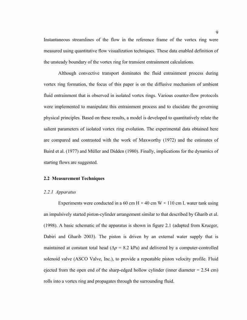
Experiments were conducted in a 60 cm H × 40 cm W × 110 cm L water tank using
an impulsively started piston-cylinder arrangement similar to that described by Gharib et al.
(1998). A basic schematic of the apparatus is shown in figure 2.1 (adapted from Krueger,
Dabiri and Gharib 2003). The piston is driven by an external water supply that is
maintained at constant total head (∆p = 8.2 kPa) and delivered by a computer-controlled
solenoid valve (ASCO Valve, Inc.), to provide a repeatable piston velocity profile. Fluid
ejected from the open end of the sharp-edged hollow cylinder (inner diameter = 2.54 cm)
rolls into a vortex ring and propagates through the surrounding fluid.

10
Figure 2.1 Schematic of apparatus for piston-cylinder experiments (adapted from Krueger et al. 2003).
A modification to the traditional piston-cylinder arrangement was made by
enclosing the primary cylinder in a 12 cm diameter coaxial shroud. An external pump
(Leeson Electronic Corp.) connected to the shroud drives flow around the primary cylinder
in either a co-flowing (co) or counter-flowing (cn) configuration. Flow conditioning
screens ensure nominally uniform flow around the primary cylinder. The shroud flow is
also regulated by a computer-controlled solenoid valve. Tests verified that the presence of
the shroud did not affect the observable vortex dynamics.
Ultrasonic flow probes (Transonic Systems, Inc.) measure the flow rates in the
cylinder and shroud. All flow data are recorded to a computer hard disk via a LabVIEW
(National Instruments) program. The starting jet flows are visualized quantitatively using
digital particle image velocimetry (DPIV, cf. Willert and Gharib, 1991). The water tank is
seeded with 13-micron (nominally) glass spheres that reflect light at the incident
wavelength. Illumination is provided by a double-pulsed Nd:YAG laser (New Wave

11 Research) that delivers 30 mJ of energy per pulse at 532 nm. The laser beam is collimated
by a cylindrical lens before entering the test section, which measures approximately 12 cm
radially and 20 cm axially downstream of the vortex generator exit plane.
Mie scattering from the seeded water is captured by a 1024 × 1024 pixel black-and-
white CCD digital camera (Uniq Vision, Inc.) at 30 Hz. The pixel resolution corresponds to
a physical test section resolution of approximately 0.19 × 0.19 mm. This is sufficient to
resolve the vortex ring core vorticity distribution. Image data are transferred in real time by
a progressive scan protocol to a frame grabber (Coreco Imaging) linked to a PC.
Images are paired according to the method described by Willert and Gharib (1991).
In the present case, each pair of images represents a separation of 18 ms between laser
pulses. This timing results in an average particle shift of 4-7 pixels between images for the
nominal piston speed of 5.5 cm s-1. Interrogation is accomplished using a window size of
32 × 32 pixels with a 50% overlap. Calculations of velocity and vorticity fields are
completed using an in-house code on an Intel 2-GHz processor. Velocity and vorticity
measurements possess an uncertainty of 1% and 3%, respectively. A MATLAB (The
Mathworks, Inc.) algorithm was created to rapidly visualize the instantaneous streamlines
of the flow, based on the measured velocity field.
The flow Reynolds number is 1400 based on the piston speed and cylinder exit
diameter, and varies between 2000 and 4000 based on the ring circulation (i.e., loop
integral of measured velocity along a path enclosing the vortex).
2.2.2 Counter-flow protocols
A variety of counter-flow protocols were implemented to manipulate the dynamics
of vortex rings generated by the piston-cylinder apparatus. The primary goal of these
12 protocols was to maintain the vortex rings in the test section for sufficient time to permit
transient fluid entrainment measurements after initial ring formation. In addition, several of
the protocols were used to affect the vorticity distribution of the rings via the dynamics of
the shear layer efflux from the vortex generator. The strength and convective velocity of
the shear layer were affected by the counter-flow, increasing the former and decreasing the
latter. These effects resulted in a modified vorticity distribution in the vortex ring. The
dynamics of the entrainment process were significantly altered by changing the vorticity
distribution in some cases, as will be shown in section 2.3.
In the absence of counter-flow, vortex ring pinch-off (i.e., dynamic separation from
the vortex generator flow source, cf. Gharib et al., 1998) was observed to occur at a
formation number F = 3.6, where
D
L
D
tUF
p offpinchoffpinch −− == . (2.2.1)
In (2.2.1), pU is the running average of the piston velocity, L is the total piston
stroke length (i.e., at the end of fluid ejection), D is the cylinder exit diameter, and t is time
measured relative to the start of piston motion. Hence, counter-flow protocols initiated
prior to L/D = 3.6 affected the vortex ring vorticity distribution, whereas those initiated
subsequent to pinch-off could not.
The magnitude of the counter-flow was assigned one of two values. In the first case
it was matched to the measured vortex ring propagation speed Uv in the absence of counter-
flow. This enabled vortex rings to be maintained at a single axial location for longer
periods of time. Alternatively, the counter-flow was set to one-half of the nominal piston
speed. This is the theoretical vortex ring propagation speed predicted by the slug model

13 (Baird et al., 1977). Table 2.1 lists the set of counter-flow protocols utilized in these
experiments, along with an abbreviated notation to be used in the following sections. The
basic format of the notation is [vortex generator L/D]-[counter-flow speed]-[initiation
delay].
Notation Vortex generator L/D Counter-flow speed Initiation Delay
LD2-CF0 2 0 N/A
LD2-CF05-12 2 0.5Up 12 L/D
LD2-CFE 2 Uv|CF0 0
LD4-CF0 4 0 N/A
LD4-CF05-2 4 0.5Up 2 L/D
LD4-CF05-6 4 0.5Up 6 L/D
LD4-CFE 4 Uv|CF0 0 Table 2.1 Counter-flow protocols.
2.3 Results
2.3.1 Vortex ring trajectories
Figure 2.2 plots the trajectories of vortex rings generated using the protocols in
table 2.1, as measured from the location of peak vorticity in the ring. In the absence of
counter-flow, cases LD2-CF0 and LD4-CF0 exhibit the expected ring propagation axially
away from the vortex generator under self-induced velocity. The additional shear layer
strength and concomitant circulation increase generated in cases LD2-CFE and LD4-CFE
(i.e., due to counter-flow initiation prior to vortex ring pinch-off) enables these vortex rings
to emerge from the vortex generator, despite the presence of counter-flow equal to Uv|CF0.
The increased circulation in the LD4-CFE case is greater than that in the LD4-CF05-2
protocol, leading to the observed larger axial translation away from the vortex generator.

14 Vortex rings generated under the protocols with larger counter-flow initiation delays (i.e.,
LD2-CF05-12 and LD4-CF05-6) exhibited abrupt changes in vortex ring trajectory due to
the sudden application of a relatively large counter-flow.
Figure 2.2 Measured vortex ring trajectory for each counter-flow protocol. (a) L/D = 2; (b) L/D = 4.

15 In each of the counter-flow protocols, a trend can be observed at later times in
which the counter-flow dominates the self-induced velocity of the rings, convecting the
vortex ring structure back toward the vortex generator. This effect can be attributed to the
increasing mass of fluid in the vortex bubble as the entrainment process proceeds, slowing
and ultimately reversing the forward progress of the bubble.
The darkened portion of each vortex ring trajectory in figure 2.2 will be the focus of
the following investigations. In these regions the vortex ring can be considered isolated,
and the transients associated with the formation process (e.g., fluid convection from the
vortex generator) have ceased.
2.3.2 Fluid entrainment and vorticity distribution
Measurements of transient fluid entrainment and vorticity distribution in isolated
vortex rings were made using DPIV. The primary difficulty associated with such
measurements—definition of the vortex boundaries—was overcome by making use of
instantaneous streamlines of the flow determined from DPIV velocity field results and a
post-processing algorithm created for this purpose.
An example of the instantaneous streamlines measured from a steadily translating
vortex ring (protocol LD2-CF0, time T = 5.34 s) is shown in figure 2.3(a), in a laboratory
reference frame. The physical extent of the vortex is not evident until the measurement is
taken in a frame moving with the ring. This was accomplished by superimposing a free-
stream axial flow with magnitude equal to the measured ring axial velocity. Figure 2.3(b)
shows the same vortex ring in its moving frame. Its physical extent is well-defined.

16
Figure 2.3 Instantaneous streamlines for protocol LD2-CF0 at time T = 5.34 s. (a) Laboratory frame; (b) vortex ring frame. Flow is from left to right.
The ring velocity was measured from the axial location of peak vorticity in the
cores. A more correct measurement should use an ad hoc vorticity centroid location, such
as that suggested by Saffman (1970). However, the difference between Saffman’s vorticity
centroid location and the vorticity peak appears to remain within experimental error.
The volume of the vortex bubble was computed using an ellipsoidal fit
based on the measured locations of the front and rear stagnation points as well as the radial
extent of the ring. In the event that the rear stagnation point was obscured (e.g., when in
close proximity to the vortex generator), this point was defined as the mirror image of the
( )tBΩ

17 front stagnation point relative to a plane containing the vortex core centers and oriented
normal to the axial direction.
Given the measured volume of the vortex bubble and the fluid volume
supplied by the vortex generator,
( )tBΩ
( )tJΩ
( ) ( )∫=t
pJ UDt0
2
d4
ττπΩ , (2.3.1)
the magnitude of entrainment was quantified by the entrained fluid fraction η(t), where
( ) ( ) ( )( )
( )( )tt
ttt
tB
J
B
JB
ΩΩ
ΩΩΩ
η −=−
= 1 . (2.3.2)
Measurements possess an uncertainty of 8% to 10%. The primary source of error
lies in the measured instantaneous vortex ring velocity that is used to visualize the
streamlines in the moving ring frame. This velocity measurement has a first-order effect on
the observed location of the ring stagnation points when the free-stream velocity is
superimposed.
Figure 2.4 plots the entrained fluid fraction η(t) measured during the darkened
portion of each vortex ring trajectory in figure 2.2. The trends are generally monotonic in
favor of increasing bubble volume. Oscillations in the measured data for protocol LD4-
CF05-2 were suspected to be due to rotation of its non-circular vortex cores, which tended
to distort the measurement of the radial vortex ring extent. This was confirmed by
examination of the vorticity contours, which indicated that the frequency of measurement
oscillation exactly matched the frequency of the non-circular core rotation.

18
Figure 2.4 Measured entrainment fraction η(t) for each counter-flow protocol. (a) L/D = 2; (b) L/D = 4.
It is immediately evident that an extrapolation of the entrainment data to time T = 0
will not lead to the expected condition of zero entrainment fraction at the start of vortex
ring formation. This is because convective fluid entrainment is the dominant mechanism at
early times, as the generated vortex sheet involutes and captures a substantial portion of

19 ambient fluid near the exit plane of the vortex generator. This captured fluid persists in the
vortex bubble indefinitely. The data collected in figure 2.4 only capture the integrated
effect of this early entrainment phase, essentially as an initial condition for the diffusive
fluid entrainment of the isolated vortex rings studied here. The dynamics of the convective
entrainment process during vortex ring formation are beyond the scope of this paper,
although it is interesting to observe in passing that the counter-flow appears to also have a
measurable effect on early convective entrainment at the stroke ratio L/D = 4.
In the absence of counter-flow, the magnitude of fluid entrainment at both piston
stroke-to-diameter ratios L/D = 2 and L/D = 4 was found to lie between 30% and 40% of
the bubble volume. These values are higher than those predicted based on a slug model
analysis similar to that of Baird et al. (1977). The discrepancy arises due to overestimation
of the vortex ring velocity by a boundary-layer-corrected slug model (e.g., Shusser et al.
2002; Dabiri and Gharib 2004a), leading to underestimation of the bubble mass that must
share the conserved impulse. The experimental result by Müller and Didden (1980) of a
40% entrained fluid fraction lies within the range observed here. A time-dependent trend in
the fluid entrainment is not reported by Baird et al. (1977) or Müller and Didden (1980),
limiting any further comparison.
Imposition of a counter-flow was demonstrated to substantially affect fluid
entrainment for several of the protocols. An entrainment fraction of nearly 65% was
observed for the LD2-CFE case, nearly 200% of the entrainment level for vortex rings
generated in the absence of counter-flow. Examination of the vorticity distribution
generated by each of the protocols provides the insight necessary to explain the mechanism

20 whereby the process of fluid entrainment is being manipulated. This will be demonstrated
in the following development.
An important parameter in the entrainment mechanism described by Maxworthy
(1972) is the spatial distribution of vorticity relative to the translating vortex bubble. It is
vorticity that has diffused outside the bubble that will reduce the total pressure of ambient
fluid near the ring (i.e., by viscous dissipation) to an extent that entrainment can proceed.
This relationship can be visualized quantitatively, by superimposing the measured vorticity
field on instantaneous streamlines of the flow in the vortex reference frame. Figure 2.5
plots these data for the protocol LD2-CF0 at times T = 1.67 s, 3.54 s, and 5.34 s. The gray
patches represent regions of vorticity magnitude above 10% of peak vorticity (10 s-1) in the
cores.
Consistent with the model of Maxworthy (1972), the vorticity diffuses beyond the
radial extent of the vortex bubble where it will interact with ambient fluid. The thickness of
this interacting layer remains steady as the vortex bubble translates, as indicated by the
plots at three distinct times during the ring evolution. A similar structure is observed in
vortex rings generated by the other protocols. The various counter-flow protocols can be
distinguished by observing the evolution of the vorticity profiles in time. Figure 2.6 shows
this evolution for cases LD2-CF0 and LD2-CFE. The vorticity profile evolution for vortex
rings generated in the absence of counter-flow (i.e., LD2-CF0) exhibits broadening of an
initially Gaussian vorticity distribution. In the process, the location of peak vorticity
remains essentially stationary, with a small movement toward the vortex ring axis of
symmetry. Thus, relative to the growing vortex bubble, the location of peak vorticity is
moving away from the ambient fluid on the opposite side of the bounding streamsurface.

21 By contrast, as the vortex rings generated by protocol LD2-CFE grow, the peak vorticity
does not decay as rapidly and its location moves radially away from the vortex ring axis of
symmetry (figure 2.6b). These effects should enhance the strength of vorticity in the
dissipation region, amplifying ambient fluid entrainment. The measurements shown in
figure 2.4 confirm this prediction.
Figure 2.5 Instantaneous streamlines and vorticity patches for protocol LD2-CF0. (a) T = 1.67 s; (b) T = 3.54 s; (c) T = 5.34 s. Minimum vorticity level is 1 s-1.

22
Figure 2.6 Measured vortex ring core vorticity profiles. (a, b) Temporal evolution of vortex ring vorticity profile for protocols LD2-CF0 and LD2-CFE, respectively; (c)
vorticity profiles for protocols LD4-CF0 and LD4-CFE at time T = 2.0 s.

23 If this physical mechanism is consistent, one can also anticipate that thicker
vortex rings—with broader vorticity distribution reaching closer to the bounding
streamsurface—will also have enhanced fluid entrainment, relative to a vortex ring with
similar aspect ratio but sharper vorticity decay in the radial direction. This, too, is confirmed
in the measurements, as indicated by comparison of the vorticity profiles of protocols LD4-
CF0 and LD4-CFE in figure 2.6(c) and their corresponding entrainment measurements in
figure 4.
An additional dynamical process becomes important to the fluid entrainment
mechanism for vortex rings generated at piston stroke-to-diameter ratios L/D greater than
the formation number F. Under these conditions, it has been demonstrated in experiments
(Gharib et al., 1998), models (Kelvin, 1875; Benjamin, 1976; Mohseni and Gharib, 1998;
Mohseni 2001), and numerical simulations (Mohseni, Ran and Colonius 2001) that the
vortex ring possesses maximum energy with respect to impulse-preserving rearrangements
of the vorticity. The vortex ring cannot accept additional fluid from the vortex generator
without violating this energy maximization, leading to the observed pinch-off. Shusser and
Gharib (2000) provide an equivalent statement of this maximization principle and predict
that pinch-off occurs when the velocity of fluid from the vortex generator falls below that
of the translating ring. Since the velocity of the ambient fluid is less than that of the vortex
generator fluid trailing behind the ring, ambient fluid entrainment must also be prohibited
after vortex ring pinch-off.
This absence of fluid entrainment is observed for protocols LD4-CF0 and LD4-
CF05-6, in which the stroke length-to-diameter ratio of the vortex generator (L/D = 4) is
greater than the formation number (F = 3.6). The entrained fluid fraction is unchanged

24 from its value at the end of the convective entrainment process (i.e., at vortex ring pinch-
off). Interestingly, we do observe substantial fluid entrainment for protocols LD4-CF05-2
and LD4-CFE well above the formation number F, despite the fact that these rings were
generated at the same L/D as the non-entraining vortex rings. The apparent contradiction is
resolved by the observation that the vortex rings generated by protocols LD4-CF05-2 and
LD4-CFE do not experience pinch-off. The effect of counter-flow on the shear layer
dynamics is to delay vortex ring pinch-off (Dabiri and Gharib 2004b). Only a minor delay
in pinch-off was necessary in the present case, since the stroke length-to-diameter ratio of
the vortex generator is only slightly greater than the formation number. However, the delay
was sufficient to prevent pinch-off and facilitate fluid entrainment. By contrast, the
counter-flow implemented in protocol LD4-CF05-6 was initiated after the formation
number and therefore could not affect the shear layer dynamics or the pinch-off process.
2.4 Comparison with Maxworthy (1972)
The work of Maxworthy (1972) provides the most complete analysis of the
diffusive entrainment process in isolated vortex rings that exists in the literature. Due to
limitations in the experimental techniques employed therein, many of the model predictions
could not be validated. Experiments conducted here are sufficient to revisit those analyses
and make detailed comparisons. The most important predictions made by Maxworthy
(1972) are a -1 power-law decay in the vortex ring propagation velocity Uv, a -2/3 power-
law decay in vortex ring circulation Γ, and the formation of a small wake behind the vortex
ring. It is prudent to note that the equivalent piston stroke-to-diameter ratio L/D in the
experiments of Maxworthy (1972) is not known. However, given that pinch-off is not

25 observed in that study and the Reynolds numbers are in the laminar regime, a
comparison with the current results is warranted.
Figure 2.7 Measured vortex ring velocity for each counter-flow protocol. (a) L/D = 2; (b) L/D = 4.
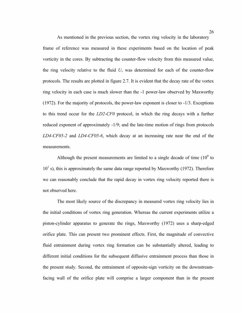
26 As mentioned in the previous section, the vortex ring velocity in the laboratory
frame of reference was measured in these experiments based on the location of peak
vorticity in the cores. By subtracting the counter-flow velocity from this measured value,
the ring velocity relative to the fluid Uv was determined for each of the counter-flow
protocols. The results are plotted in figure 2.7. It is evident that the decay rate of the vortex
ring velocity in each case is much slower than the -1 power-law observed by Maxworthy
(1972). For the majority of protocols, the power-law exponent is closer to -1/3. Exceptions
to this trend occur for the LD2-CF0 protocol, in which the ring decays with a further
reduced exponent of approximately -1/9; and the late-time motion of rings from protocols
LD4-CF05-2 and LD4-CF05-6, which decay at an increasing rate near the end of the
measurements.
Although the present measurements are limited to a single decade of time (100 to
101 s), this is approximately the same data range reported by Maxworthy (1972). Therefore
we can reasonably conclude that the rapid decay in vortex ring velocity reported there is
not observed here.
The most likely source of the discrepancy in measured vortex ring velocity lies in
the initial conditions of vortex ring generation. Whereas the current experiments utilize a
piston-cylinder apparatus to generate the rings, Maxworthy (1972) uses a sharp-edged
orifice plate. This can present two prominent effects. First, the magnitude of convective
fluid entrainment during vortex ring formation can be substantially altered, leading to
different initial conditions for the subsequent diffusive entrainment process than those in
the present study. Second, the entrainment of opposite-sign vorticity on the downstream-
facing wall of the orifice plate will comprise a larger component than in the present

27 experiments. Maxworthy (1972) predicts the production and convection of this opposite-
sign vorticity to affect the dynamics of the evolving vortex rings. It is possible that the
translational velocity of the rings is one of the affected parameters, e.g., by vorticity
cancellation in the ring, which will reduce its self-induced velocity. The effect of opposite-
sign vorticity is further amplified for vortex rings generated at small L/D, in which the
relative fraction of opposite-sign vorticity increases.
To predict a temporal trend in the vortex bubble circulation, Maxworthy (1972)
uses a model that assumes the vortex ring possesses a nominally constant impulse. The
model is admittedly limited to large Reynolds numbers and small time scales, so that
impulse loss to the wake behind the ring can be neglected. Nevertheless, a -2/3 power-law
decay rate in the ring circulation is predicted. Figure 2.8 plots the temporal trends in ring
circulation for the protocols tested in these experiments. The decay rates are much slower
than predicted by Maxworthy (1972). Specifically, the protocols using L/D = 2 decay with
a power-law exponent an order of magnitude smaller than that observed by Maxworthy
(1972). The circulation of thicker vortex rings at L/D = 4 decays slightly faster, but still at a
rate much smaller than the -2/3 power-law.
It is likely that this discrepancy is due to the fact that the present experiments satisfy
neither the requirement of large Reynolds number, nor the assumption of short elapsed
time. Hence it is also incorrect to assume a constant impulse for the vortex ring.

28
Figure 2.8 Measured vortex ring circulation for each counter-flow protocol. (a) L/D = 2; (b) L/D = 4. Note that the data symbol convention in (b) has been altered
to avoid data point overlap.

29 Using the analytical method of Maxworthy (1972), one can attempt to estimate
the decay rate of the ring impulse based on the measured ring velocity and circulation. The
impulse I is related to the ring circulation Γ and the characteristic dimension of the vortex
bubble 31BΩ by
321 BCI ΓΩ= , (2.4.1)
where C1 is a dimensionless constant dependent on the bubble shape. The vortex ring
velocity Uv is related to the ring circulation Γ and the characteristic bubble dimension 31BΩ
by
312B
v CUΩΓ
= , (2.4.2)
where C2 is also a dimensionless constant dependent on the bubble shape. Therefore the
ring impulse goes as
2
3
~vU
I Γ . (2.4.3)
Substituting the measured -1/3 power-law decay for the vortex ring velocity and
-1/10 power-law decay for the vortex ring circulation (conservatively), the ring impulse is
actually predicted to increase with an 11/30 power-law in time! This physically incorrect
result of increasing impulse also holds for each of the protocols when the individual
velocity and circulation decay rates are input to (2.4.3) in place of the nominal values
above. Therefore we must re-examine the model of Maxworthy (1972). Specifically, the
following section will show that the non-physical result arises due to the assumption of
self-similar vortex bubble growth that is implicit in the use of constant parameters (e.g., C1
and C2) to relate the characteristic ring dimension to the actual bubble shape.

30 Before concluding this section, it is useful to explore the final important
prediction of Maxworthy (1972), namely the formation of a wake behind the vortex ring.
Figure 2.9 plots the vorticity patches and instantaneous streamlines for a vortex ring formed
using protocol LD2-CF0 at time T = 5.74 s. The minimum vorticity level has been reduced
to 3% of the peak vorticity in the vortex core in order to visualize regions of low vorticity.
As this represents the upper-bound on the measurement error, the data must be interpreted
with caution, especially in regions of the flow with large velocity gradients. Nevertheless,
the measurement does appear to capture the presence of symmetric vorticity patches behind
the vortex ring, in accordance with the prediction of Maxworthy (1972). The existence of
this wake structure emphasizes the fact that the increase in vortex ring impulse predicted by
the model above must be incorrect. Given the consistency of the observed wake with the
aforementioned physical mechanism for diffusive fluid entrainment proposed by
Maxworthy (1972), it will henceforth be assumed correct and will be used in the following
section to derive an improved quantitative model for the process.
Figure 2.9 Instantaneous streamlines and vorticity patches for protocol LD2-CF0. Time T = 5.74 s. Minimum vorticity level is 0.3 s-1.

31 2.5 A Quantitative Model for Diffusive Fluid Entrainment
The physical process of diffusive entrainment is assumed to be essentially that of
Maxworthy (1972), as described in the Introduction. Our model will make the corollary
assumption that the fraction of ambient fluid flux into the dissipation region that is
entrained by the vortex ring is proportional to the fraction of energy lost by the ambient
fluid in the same region, i.e.,
tEtE
tt
I
L
D
B
dddd~
dddd
ΩΩ , (2.5.1)
where tB ddΩ is the flux of entrained fluid from the dissipation region into the vortex
ring, dtDΩd is the total flux of fluid into the dissipation region, tEL dd is the rate of
ambient fluid energy loss due to viscous dissipation in the dissipation region, and tEI dd
is the rate of ambient fluid energy entering the dissipation region.
The rate of energy loss tEL dd (per unit mass) is computed using the two-
dimensional incompressible dissipation function Φ in the energy equation (i.e., the scalar
product of the momentum equation with the velocity vector u; see Batchelor (1967):
∂∂
+∂∂
+
∂∂
+
∂∂
==222
212
dd
ru
xv
rv
xu
tEL νΦ , (2.5.2)
where u and v are the velocity components in the axial x and radial r directions,
respectively. The magnitude of the dissipation function will be proportional to the
kinematic viscosity ν, and to a characteristic speed Uv and length scale 31BΩ over which
changes in fluid velocity occur, i.e.,

32
3221d
d −== BvL US
tE
ΩνΦ . (2.5.3)
In (2.5.3), S1 is a dimensionless shape factor that is dependent on time and other
parameters to be delineated shortly. This is distinct from the assumption of constant shape
factors used by Maxworthy (1972).
The rate of ambient fluid energy entering the dissipation region (per unit mass) is
directly proportional to the square of the fluid velocity and inversely proportional to the
time scale over which the process occurs:
12
dd −= dv
I TUt
E . (2.5.4)
This characteristic dissipation time scale Td can be replaced by the characteristic velocity
and bubble dimension as 1312
−= vBd UST Ω , where S2 is a second dimensionless shape factor.
With this substitution, (2.5.4) becomes
3132d
d −= BvI US
tE
Ω . (2.5.5)
Finally, the volume flux of fluid into the dissipation region is
( ) 2121213
212
31213d
dvBvBd
D USSUTSt
ΩνΩνΩ
== , (2.5.6)
where the radial extent of the dissipation region is proportional to ( ) 21dTν . Substituting
(2.5.3), (2.5.5), and (2.5.6) into (2.5.1) gives an expression for the vortex bubble growth as
a function of the characteristic ring velocity and dimension, and the shape factors:
6121233
2121d
dBv
B USSSt
ΩνΩ −−= . (2.5.7)

33 Henceforth, we will consider a dimensionless lumped shape factor 3
2121 SSS −=S
and unit viscosity. As mentioned above, the shape factor is no longer assumed constant,
and is instead dependent on time and the set of parameters that will affect the shape and
size of the ring from the start of diffusive entrainment: the instantaneous circulation of the
ring Γ(t); the duration of vortex generator fluid ejection Te; the rate of change of the
entrained fluid fraction dη/dt; and the vortex generator exit diameter D. Given this
functional dependence, the shape factor can be expressed in terms of a single dimensionless
parameter,
tTDt
SS e2
ddˆ −= Γη , (2.5.8)
where is a dimensionless constant. Substituting for S in (2.5.7) using this result and
rearranging with the use of (3.2), we obtain
S
( ) ( ) ( ) 11611311611611121160 ~ ttUTDtSt vJeBB−−+= ΩΓΩΩ . (2.5.9)
Note that (2.5.9) is dimensionally correct with 116ˆ~ SS = as a dimensionless
constant, when the unit viscosity from (2.5.7) is included. The time variable t in (2.5.9) is
measured relative to the beginning of diffusive entrainment. Therefore the constant is
included as the volume of the vortex bubble at the beginning of the diffusive entrainment
phase. The magnitude of will be determined by the dynamics of the preceding
convective entrainment phase. In the following, will be estimated based on the earliest
data points in each measurement series, although it is recognized that each measurement
did not necessarily commence immediately after the convective entrainment phase.
0BΩ
0BΩ
0BΩ

34 The large number of parameters in (2.5.9) may be reduced via simplifying
assumptions regarding the dependence of the vortex ring velocity Uv(t) on its circulation
(e.g., Norbury, 1973), and the dependence of the circulation on the variables , D, and
T
JΩ
e (e.g., slug model approximation, cf. Shariff and Leonard, 1992). However, since the data
for every parameter are readily available in the present case, we will not implement those
approximations at this time.
Figure 2.10 plots the predicted vortex bubble growth law in (2.5.9) for each of the
counter-flow protocols (excluding the non-entraining protocols LD4-CF0 and LD4-CF05-
6), along with the measured vortex bubble growth in each case. The shape constant for each
curve is indicated in the figure. A consistently high level of agreement is observed in each
case, with the exception of the late-time behavior of protocol LD2-CFE. This discrepancy
is probably due to the close proximity of the ring to the vortex generator, as indicated by its
trajectory in figure 2.2. It appears that the vortex generator may have prevented normal
deposition of ring circulation into a wake, allowing the ring to achieve substantially
enhanced entrainment at later times when the ring circulation is normally decaying. This
explanation is supported by the observed lack of ring circulation decay for protocol LD2-
CFE in figure 2.8. Although this result emphasizes the role of vorticity distribution in the
entrainment process, these modified entrainment dynamics cannot be captured by the
current model.
The dimensionless shape constant is of order unity and exhibits only modest
variation across the range of experimental results. It appears that the constant scales with
increasing entrainment enhancement, but the current data are insufficient to draw firm
conclusions.
S~

35
Figure 2.10 Comparison of predicted vortex growth to experimental measurements. Non-entraining protocols (i.e., LD4-CF0 and LD4-CF05-6) are excluded.
2.6 Conclusions
Novel experimental techniques have been developed to probe the dynamics of iso-
lated vortex rings. The counter-flow protocols have enabled empirical study of vortex ring
evolution in a moving frame of reference, effectively eliminating many of the common
obstacles to progress in previous efforts. Quantitative velocimetry has elucidated the
structure of the rings, and a diverse set of experimental conditions has indicated the special
role of vorticity distribution and vortex ring pinch-off in the diffusive process of ambient
fluid entrainment. In a normal diffusive process (i.e., without counter-flow enhancement),
entrained fluid fractions between 30% and 40% were measured. Various counter-flow
protocols demonstrated the possibility of substantial entrainment augmentation, up to a
65% entrained fluid fraction in these experiments.

36 Wake formation behind vortex rings during the entrainment process was
observed in these experiments, confirming the physical model for diffusive entrainment
suggested by Maxworthy (1972). The corresponding measurements of ring velocity and
circulation showed substantial discrepancy, however. Differences in observed ring velocity
are probably due to dissimilar boundary conditions in the vortex generator of the previous
experiments and the current study, while the overestimate in predicted circulation decay
can be attributed to the invalid assumptions of constant ring impulse and self-similar
growth in the previous analysis. The present results should serve to caution efforts to
describe vortex ring dynamics using constant-impulse or constant-volume assumptions.
Although such approximations may be reliable early in the diffusive stage of fluid
entrainment, they are inappropriate during both ring formation and late-time ring
propagation.
A model for diffusive fluid entrainment has been developed here that does not
assume a self-similar shape for vortex rings as they evolve, nor does it require a nominally
constant ring impulse. Dimensional analysis and physical arguments were used to derive
the growth rate of the vortex bubble as a function of ring circulation and propagation speed.
Predictions of the model were found to agree well with measurements of the normal
diffusive entrainment process, and it is hypothesized that the shape constant may scale
with increasing entrainment enhancement. Unfortunately, the discovery that the vortex
rings do not evolve self-similarly limits our ability to predict trends in the ring impulse
using formulae from thin-core approximations or steady solution families (e.g., Fraenkel,
1972; Norbury, 1973).
S~

37 Future efforts must be directed toward achieving a better understanding of the
rapid convective entrainment process that occurs during vortex ring formation. One can
infer from the present experiments that this early phase of entrainment will be responsible
for much of the entrained fluid fraction that persists in the vortex rings. The current
experimental method was not sufficiently accurate to resolve that convective entrainment
process, but it is possible that a refinement of the technique introduced here might be
effective. Despite the absence of dynamical information regarding the convective fluid
entrainment process, the present experiments have definitively shown a substantial
contribution of ambient fluid entrainment to the dynamics of vortex rings. As improved
ideal vortex ring models are being developed, it will be prudent to account for this
phenomenon.
These results may have important implications for pulsed jet systems that possess a
capability to manipulate the vortex ring velocity and/or vorticity distribution.
Notwithstanding the many manmade applications that may be designed to exploit these
parameters in the future, various animals may have already achieved success in this
endeavor. For example, it is known that many pulsed-jet animal swimmers that are
dependent on self-generated vortical flows for feeding are narrowly tuned for a specific
swimming speed regime. Since the relative speed of vortex rings generated during
swimming is coupled to the prevalent swimming speed regime of the animal, it will be
interesting to further examine the relationship between swimming regime and the
effectiveness of entrainment mechanisms in these animals.

38 2.7 Chapter References
Baird, M. H. I., Wairegi, T. and Loo, H. J. 1977 Velocity and momentum of vortex rings in
relation to formation parameters. Can. J. Chem. Engng. 55, 19-26.
Batchelor, G. K. 1977 An Introduction to Fluid Dynamics. Cambridge University Press.
Benjamin, T. B. 1976 The alliance of practical and analytical insights into the non-linear
problems of fluid mechanics. In Applications of Methods of Functional Analysis to
Problems in Mechanics (ed. P. Germain and B. Nayroles). Lecture Notes in
Mathematics, vol. 503, pp. 8-28. Springer.
Dabiri, J. O. and Gharib, M. 2004a A revised slug model boundary layer correction for
starting jet vorticity flux. Theor. Comput. Fluid Dyn. 17, 293-295.
Dabiri, J. O. and Gharib, M. 2004b Delay of vortex ring pinch-off by an imposed bulk
counter-flow. Phys. Fluids 16, L28-L30.
Fraenkel, L. E. 1972 Examples of steady vortex rings of small cross-section in an ideal
fluid. J. Fluid Mech. 51, 119-135.
Gharib, M., Rambod, E. and Shariff, K. 1998 A universal time scale for vortex ring
formation. J. Fluid Mech. 360, 121-140.
Kelvin, W. T. 1875 Vortex statics. Collected Works vol. 4, pp. 115-128. Cambridge
University Press.
Krueger, P. S., Dabiri, J. O. and Gharib, M. 2003 The formation number of vortex rings
formed in the presence of uniform background co-flow. Phys. Fluids 15, L49-L52.
Liess, C. and Didden, N. 1976 Experimente zum einfluss der anfangsbedingungen auf die
instabilität von ringwirblen. Z. Angew. Math. Mech. 56, T206-T208.

39 Linden, P. F. and Turner, J. S. 2001 The formation of ‘optimal’ vortex rings, and the
efficiency of propulsion devices. J. Fluid Mech. 427, 61-72.
Maxworthy, T. 1972 The structure and stability of vortex rings. J. Fluid Mech. 51, 15-32.
Maxworthy, T. 1977 Some experimental studies of vortex rings. J. Fluid Mech. 80, 465-
495.
Mohseni, K. 2001 Statistical equilibrium theory for axisymmetric flows: Kelvin’s
variational principle and an explanation for the vortex ring pinch-off process. Phys.
Fluids 13, 1924-1931.
Mohseni, K. and Gharib, M. 1998 A model for universal time scale of vortex ring
formation. Phys. Fluids 10, 2436-2438.
Mohseni, K., Ran, H. Y. and Colonius, T. 2001 Numerical experiments on vortex ring
formation. J. Fluid Mech. 430, 267-282.
Müller, E. A. and Didden, N. 1980 Zur erzeugung der zirkulation bei der bildung eines
ringwirbels an einer dusenmundung. Stroj. Casop. 31, 363-372.
Norbury, J. 1973 A family of steady vortex rings. J. Fluid Mech. 57, 417-431.
Prandtl, L. and Tietjens, O. G. 1934 Fundamentals of Hydro and Aeromechanics. Dover.
Reynolds, O. 1876 On the resistance encountered by vortex rings, and the relation between
vortex rings and the streamlines of a disk. Nature 14, 477.
Saffman, P. G. 1970 The velocity of viscous vortex rings. Stud. Appl. Maths 49, 371-380.
Shariff, K. and Leonard, A. 1992 Vortex rings. Annu. Rev. Fluid Mech. 24, 235-279.
Shusser, M. and Gharib, M. 2000 Energy and velocity of a forming vortex ring. Phys.
Fluids 12, 618-621.

40 Shusser, M., Gharib, M., Rosenfeld, M. and Mohseni, K. 2002 On the effect of pipe
boundary layer growth on the formation of a laminar vortex ring generated by a
piston/cylinder arrangement. Theor. Comput. Fluid Dyn. 15, 303-316.
Widnall, S. E. and Sullivan, J. P. 1973 On the stability of vortex rings. Proc. R. Soc. Lond.
A 332, 335-353.
Willert, C. E. and Gharib, M. 1991 Digital particle image velocimetry. Exps. Fluids 10,
181-193.
41
CHAPTER 3: A contribution from wake vortex added-mass in estimates of
animal swimming and flying dynamics
Submitted to Journal of Experimental Biology February 10, 2005
3.0 Chapter Abstract
Wake analyses are currently the most popular method for studying the dynamics of
swimming and flying animals. The effect of the wake vortex structures on locomotion is
typically deduced based solely on their rotational momentum. We conduct a case study of
the vortex wake generated by free-swimming Aurelia aurita jellyfish, as well as a
mechanical device that mimics their jetting system, to demonstrate the existence of an
additional and substantial dynamical contribution from the irrotational added-mass of the
wake vortices. This added-mass contribution is separate from the effects encountered due
to acceleration of the animal body and its appendages. These fluid vortex added-mass
dynamics are neglected in current methods of quantitative wake analysis, but should be
included in order to achieve accurate estimates of locomotive dynamics.
3.1 Introduction
The vortex wake is the fluid dynamical signature of swimming and flying animals.
It can be studied to infer net thrust or drag in an accelerating animal or probed to determine
the relative contributions to lift and forward motion in steady locomotion.
Current studies of wake vortex dynamics focus on the rotational momentum of the
vortices. The magnitude of rotational momentum in the region V downstream from the
animal can be determined from the vorticity distribution ω via the hydrodynamic ( )x

42 impulse in the flow, defined as . This integral of the first moment of
vorticity is then related to non-conservative external forces F acting on the flow by the
equation
∫ × d~ ωxI V
∫= dVt FI dd (Saffman, 1992). When discrete vortices arise in the wake, current
models of their dynamics will either use these formulae directly, or apply simplifying
approximations regarding the distribution of vorticity and its evolution in time (cf. Shariff
and Leonard, 1992).
An additional irrotational added-mass contribution to vortex wake momentum has
been previously proposed (Weihs, 1977; Sunada and Ellington, 2001). In the simplified
analytical treatment of unsteady jet flow by Weihs (1977), it was suggested that coherent
ring vortex structures in the flow would exhibit dynamic behavior similar to solid bodies
with equivalent geometric dimensions. In particular, the fluid structures would exhibit an
added-mass effect in which fluid external to the vortices experiences a net drift in the
direction of ring vortex translation without actually being entrained into the vortices. This
effect was quantified using an added-mass coefficient CAM, which represents the volume of
external fluid drifting downstream with the vortex, as a fraction of the total vortex volume.
The coefficient is identical in definition to the index typically used to characterize
accelerating solid bodies during swimming and flying motions (e.g., Batchelor, 1967;
Daniel, 1984; Dickinson et al., 1999).
Recently, the first empirical measurements of vortex dynamics in a similar unsteady
jet flow showed that the impulse delivered to the flow in the form of fluid vortices cannot
be fully accounted by considering only the rotational momentum (Krueger and Gharib,

43 2003). They, too, hypothesized that the effects of wake vortex added-mass might play a
role.
Despite a rich literature dealing with the added-mass of animal bodies and their
appendages, the question of whether fluid vortices such as those observed in animal vortex
wakes actually exhibit added-mass behavior has not been previously resolved. The induced
Lagrangian fluid particle drift (i.e., tracking individual fluid elements) necessary to
generate an added-mass effect in vortex flows has not been quantified in any previous
study. Hence, the existence of a fluid vortex added-mass effect similar to that observed in
solid bodies and multi-phase flows has remained an unproven conjecture.
In this paper, we use quantitative visualizations of Aurelia aurita jellyfish and a
mechanical analogue, to demonstrate an important dynamical contribution from added-
mass in the vortex wake. This phenomenon is separate from the added-mass contribution of
the animal body and appendages and is neglected in current methods of quantitative wake
analysis. The techniques described herein allow for the quantification of these missing
dynamics in the case of jellyfish swimming and can be readily extended to quantify the
wake vortex added-mass dynamics in other animals as well.
Jellyfish were selected as the focus of this proof-of-concept study because they
have been observed to form some of the simplest vortex wakes in the animal kingdom, a
train of nearly axisymmetric vortex rings (Dabiri et al., 2005). This wake structure can be
more easily replicated and quantified in controlled laboratory experiments than fully three-
dimensional vortices. Extension of these results to more complex wake structures is
proposed in the Discussion.

44 3.2 Methods
Juvenile Aurelia medusae raised at the Cabrillo Marine Aquarium (Long Beach,
California, USA) were transferred to a transparent pseudokreisel jellyfish facility at the
California Institute of Technology for quantitative flow visualization experiments using
digital particle image velocimetry (DPIV; Willert and Gharib, 1991). A 532-nm planar
laser sheet illuminated 14-µm glass beads seeded throughout the pseudokreisel saltwater
supply. These particles were quantitatively tracked to measure the instantaneous velocity
field surrounding the animals. Neither the laser sheet nor the particles were observed to
affect the swimming behavior of the jellyfish during the flow measurements. All flow
visualization data were collected from animals swimming in regions of the tank at least 2
body diameters from the side walls and 5 body diameters from the tank floor, and with their
bodies oriented approximately symmetric in the plane of the laser sheet. In addition, only
animals swimming in isolation (i.e., away from other medusae) were selected for flow
visualization.
A mechanical apparatus was constructed to simulate the observed jellyfish wake in
repeatable and controlled experiments. Specifically, wake vortex rings were generated
using a piston-cylinder apparatus (Dabiri and Gharib, 2004). The device was submerged in
water and ejected discrete pulses of fluid with jet length-to-diameter ratio L/D = 2 from the
open end of a hollow 2.54-cm diameter circular tube. During each pulse, the free shear
layer produced by the vortex generator rolled into a single ring vortex that propagated
downstream via its self-induced motion. The downstream velocity field created by the
vortex generator was measured using the same DPIV technique applied to the free-

45 swimming jellyfish. All velocity field measurements possess an uncertainty between 1%
and 3%, with larger uncertainty occurring in regions with greater spatial velocity gradients.
To determine the Lagrangian particle drift induced by the translation of the
generated wake vortices, several sets of “virtual” particles were seeded in the measured
vortex generator flow. Prior to wake vortex formation, the particles were initialized with
positions in the flow corresponding to several discrete, axisymmetric, planar discs
downstream of the vortex generator, each oriented normal to the direction of downstream
propagation of the wake vortex rings. Since the DPIV data is two-dimensional, these
axisymmetric planes correspond to straight lines in the measured two-dimensional flow,
i.e., the planes are viewed in a meridian cross-section. The motion of each planar set of
particles was determined by updating the positions of those particles based on the measured
instantaneous Eulerian velocity fields from DPIV. Cubic interpolation was used to
determine the local velocity to sub-grid resolution.
3.3 Results
Figure 3.1(a) shows the measured vortex wake of a swimming Aurelia in a plane
near the radial symmetry plane of the animal. Instantaneous streamlines of the flow (i.e.,
lines tangent to local velocity vector) are used to visualize the wake. This method of
visualization is useful for determining the global topology of the flow. A pair of vortex
rings is clearly visible in the wake.
Figure 3.1(b) shows a wake vortex ring generated by the mechanical analogue. The
vortex ring is propagating downstream away from the apparatus. The topology of this wake
vortex ring flow is comparable to that produced by the real jellyfish in figure 3.1(a).
Although the mechanical apparatus does not experience an external flow as seen in the

46 reference frame of the free-swimming animals, previous studies have shown that the
vortex ring kinematics and flow topology are qualitatively consistent in the presence of
moderate external flows such as those induced during swimming (Krueger et al., 2003).
The full extent of the vortex ring was visualized using the method of Dabiri and
Gharib (2004), in which the vortex streamlines are tracked in a frame of reference moving
at the translational velocity of the vortices, rather than in the laboratory reference frame
(figure 3.1c). This latter perspective enables us to observe all of the fluid carried by the
vortex ring, information that will be necessary in the following analysis in order to properly
investigate the added-mass behavior of the vortices.
1 1
2 2
1
1
Figure 3.1 DPIV measurements of free-swimming jellyfish and a mechanical analogue. Images are taken in the laser sheet plane, which is aligned close to the
plane of symmetry of the flow. (a) Vortex wake of the free-swimming jellyfish consists of a train of nearly axisymmetric vortex rings (white arrows, cores numbered in order
of formation). Flow field is approximately 14 cm in height. (b) Vortex ring propagating downstream from the mechanical apparatus. Exit plane of the vortex
generator is located at the upper margin of the frame. Flow is vertically downward. Flow field is 20 cm in height. (c) Vortex ring from frame (b) viewed in its propagating reference frame. The full extent of the vortex is clearly visible from this perspective.
Flow field is 20 cm in height.

47 A straightforward heuristic has been previously developed to compute the added-
mass of any solid body (Darwin, 1953). As the body translates steadily through a plane of
initially stationary fluid particles in the flow (oriented normal to the direction of
translation), it will induce a net drift of the particles in the direction of body translation.
After the body has passed downstream, the volume of fluid between the distorted
plane and its initial position is equal to the product of the added-mass coefficient and the
volume of the solid body , i.e., (figure 3.2c). Proving this result as
a mathematical theorem requires care (cf. Darwin, 1953; Lighthill, 1956; Benjamin, 1986;
Eames et al., 1994; Yih, 1997; Eames, 2003); however, the accuracy and robustness of this
method has been demonstrated in a variety of experimental studies (e.g., Eames and
Duursma, 1997; Bush and Eames, 1998; Eames and Flor, 1998).
driftΩ
bodyΩ bodydrift Ω=Ω AMC
The added-mass behavior of a solid sphere traveling through such a planar
collection of Lagrangian fluid particles is computed in figure 3.2, using the potential flow
stream function for a steadily translating sphere (Milne-Thompson, 1968). The reference
plane (shown in cross-section) is distorted to a horn-like shape after passage of the sphere.
Interestingly, individual fluid particles do not drift unidirectionally, but instead exhibit
looping paths referred to as elasticas (Darwin, 1953). These elasticas cause the drift
volume to undergo a temporal oscillation before achieving the asymptotic value of
0.5 , consistent with the known added-mass coefficient for a sphere. bodyΩ
Lagrangian particles in the laboratory-generated wake vortex flow were observed to
behave in a manner very similar to the inviscid sphere solution (figure 3.3). Looping
elastica paths were induced by the translating vortices, and the initially planar surfaces
48 were again distorted to horn-like shapes. To account for the fact that the translating
vortices are increasing in size as they propagate downstream (i.e., due to entrainment of
ambient fluid), several planes downstream of the vortex generator were tracked. Each
showed similar deformation patterns. The entrainment process is sufficiently slow such that
no substantial acceleration of the near wake (and accompanying virtual buoyancy, cf.
Batchelor, 1967) is observed to occur in the flow (Dabiri and Gharib, 2004).

49
Figure 3.2 Demonstration of heuristic (i.e., Darwin, 1953) for measuring solid body added-mass. Axisymmetric inviscid flow about a solid sphere is shown in cross
section. Solutions were computed using dimensional units to allow comparison with experimental results. Sphere radius and propagation speed are 2.54 cm and 1 cms-1,
respectively. Computational domain is 50 sphere radii axially in both directions normal to the reference plane and approximately 12 cm radially. Total fluid drift
(i.e., for infinite domain) was computed using measured partial drift in the computational domain and an analytical asymptotic correction factor (i.e., Eames et
al., 1994). (a) Sphere approaches initially planar Lagrangian surface from left; t = 0 s.

50 (b) Streamwise distortion of Lagrangian surface occurs as the sphere passes
through the plane; t = 4.45 s. Note that since only streamwise Lagrangian displacement is plotted, the sphere appears to pass through the plane. Plots of
combined streamwise and transverse Lagrangian displacement (e.g., (d)-(f) below) verify that the plane is actually distorted around the sphere. (c) Volume between
initial plane and horn-like distorted surface is the drift volume, Ω , from which the added-mass coefficient is computed; t = 13.3 s. (d)-(f) Individual Lagrangian particle
paths corresponding to t = 0 s, 4.45 s, and 13.3 s, respectively.
drift
Figure 3.3 Measurements of Lagrangian drift induced by translating fluid vortices. Vortex is indicated by black arrow. (a) Vortex approaches several planar Lagrangian
surfaces downstream of the vortex generator (several more planes further downstream not shown); t = 0.07 s. (b), (c) Fluid vortices interact with Lagrangian
surfaces in a manner similar to that observed for the inviscid sphere solution. Initially planar surfaces are deformed to horn-like shapes; t = 3.34 s and 13.3 s,
respectively. (d)-(f) Individual Lagrangian particle paths corresponding to t = 0.07 s, 3.34 s, and 13.3 s, respectively.

51 In addition to the volume of each fluid vortex increasing as it propagates
downstream, the asymptotic behavior of its associated drift volume also exhibits sustained
linear growth rather than saturation at a constant drift volume as was observed for the solid
body (figure 3.4). This linear growth in the drift volume reflects the fact that for the
observed constant vortex shape (and hence constant added-mass coefficient), the drift
volume will continually increase to maintain its magnitude at a constant ratio (i.e., the
added-mass coefficient) relative to the growing fluid vortex.
Figure 3.4 Drift and fluid body volume measurements for translating vortices. Colored solid lines: Drift volume of planes initially located in 0.3 cm increments from 2.7 cm (red) to 8.0 cm (blue) downstream of the vortex generator exit. Total fluid drift
(i.e., for infinite domain) was computed using measured partial drift in the measurement window and an analytical asymptotic correction factor (i.e., Eames et al., 1994). Closed circles: Measured volume of ellipsoidal fluid vortex. Error bars
indicate measurement uncertainty. Dashed blue line: Least-squares linear fit to vortex volume measurements. Solid red line: Linear fit required to exactly match the added-
mass coefficient of an equivalent solid body. Inviscid sphere solution is plotted for comparison.

52 The observed temporal growth of the propagating vortices requires that the
heuristic for computing the added-mass coefficient be modified. To properly the compute
the added-mass coefficient for fluid vortices, we must first subtract the entrained fluid from
the total drift volume, i.e., , since the entrained fluid is
already accounted for in the volume of the vortex, . In the present case (figure 3.4),
the temporal trends in each of these parameters can be measured such that the above
equation becomes 2 or, in the limit as t → ∞ (i.e., so that the
vortex has passed far downstream), C
bodyentraineddrift Ω=Ω−Ω AMC
bodyΩ
( )tt 54.1C54 AM=t .165. −
AM = 0.72. This is precisely the added-mass
coefficient for a solid ellipsoidal body with the same shape as the fluid vortices. In figure
3.4, the least-squares linear fit to the vortex volume data is compared with the linear trend
required for an exact match to the added-mass coefficient of an equivalent solid body. The
agreement is very good.
3.4 Discussion
The present results demonstrate an important contribution to vortex dynamics that
is absent from current methods of animal wake analysis, especially those utilizing
quantitative wake measurements to estimate locomotive dynamics. The added-mass
coefficient of 0.72 measured here indicates that, in addition to transporting fluid via the
translating vortices, the vortex generator also indirectly moves an additional mass of fluid
whose magnitude is 72 percent of the primary vortex. This is a very substantial
improvement in fluid transport that can have profound dynamical effects on animal
locomotion. Given the relative magnitude of this effect, it is reasonable to hypothesize that
the locomotor could not function as effectively in its absence.

53 The magnitude of the wake vortex added-mass effect demonstrated here will
vary depending on the animal of interest and its locomotive gait. Biological factors
affecting vortex formation (e.g., time-dependent boundary conditions, flexible surfaces,
etc.) will produce quantitative differences in the wake vortex added-mass effect relative to
the mechanical analogue used in these experiments. However, the physical analogy with
inviscid body added-mass suggests that the wake vortex added-mass contribution in those
cases will remain similar, both qualitatively and in order of magnitude, to the present
results.
We have focused on axisymmetric fluid vortices because their propagation is
rectilinear and hence only one component of the full added-mass tensor is required in order
to characterize their irrotational wake dynamics. Methods more advanced than the current
heuristic will be necessary to determine the additional non-zero elements of the added-mass
tensor that arise for the large class of animal vortex wakes that do not propagate
rectilinearly or unidirectionally.
Nonetheless, the basic physical concept of induced fluid particle drift that led to the
added-mass effect measured here is sufficiently general that it should also appear in more
complex animal vortex wakes. The vortex wake added-mass effect is also not limited to
swimming animals, despite the fact that the present experiments were conducted in water.
The bounding streamlines of the fluid vortices (viewed in an appropriate reference frame)
mimic the dynamical behavior of solid bodies in inviscid flow via the no through-flow
condition that holds at the boundaries; this no through-flow condition appears with equal
importance in air, water, or any other fluid medium.

54 The net contribution of the solid body added-mass dynamics to animal
locomotion typically vanishes in a time-periodic flow (Daniel, 1984). However unlike solid
bodies, fluid vortex bodies are time-varying in their volume, shape, and associated added-
mass. Since the added-mass contributions during vortex acceleration and deceleration will
not be identically equal and opposite, the net contribution to the animal swimming and
flying dynamics can be non-zero.
An important example is the wake capture mechanism observed prominently in
insect flight (e.g., Dickinson et al., 1999) and fish swimming (e.g., Liao et al., 2003). Wake
vortex added-mass provides a direct dynamical contribution to this mechanism via the
acceleration and/or deceleration of the wake vortices. When the locomotor body and/or
appendages interact with fluid vortices, the dynamics of both the vortex and the associated
added-mass of the vortex are affected (and vice versa, via Newton’s third law). How
animals effectively exploit the added-mass dynamics during these fluid-structure
interactions is an important question that mandates further study.
3.5 Chapter References
Batchelor, G. K. 1967 An Introduction to Fluid Dynamics. Cambridge University Press.
Benjamin, T. B. 1986 Note on added-mass and drift. J. Fluid Mech. 169, 251-256.
Bush, J. W. M. and Eames, I. 1998 Fluid displacement by high Reynolds number bubble
motion in a thin gap. Int. J. Multiphas. Flow 24, 411-430.
Dabiri, J. O. and Gharib, M. 2004 Fluid entrainment by isolated vortex rings. J. Fluid
Mech. 511, 311-331.
Daniel, T. L. 1984 Unsteady aspects of aquatic locomotion. Am. Zool. 24, 121-134.
Darwin, C. 1953 Note on hydrodynamics. P. Camb. Philos. Soc. 49, 342-354.

55 Dickinson, M. H., Lehmann F. O. and Sane S. P. 1999 Wing rotation and the
aerodynamic basis of insect flight. Science 284, 1954-1960.
Eames, I. 2003 The concept of drift and its application to multiphase and multibody
problems. Phil. Trans. R. Soc. Lond. A 361, 2951-2965.
Eames, I., Belcher, S. E. and Hunt, J. C. R. 1994 Drift, partial drift and Darwin’s
proposition. J. Fluid Mech. 275, 201-223.
Eames, I. and Duursma, G. 1997 Displacement of horizontal layers by bubbles injected into
fluidized beds. Chem. Eng. Sci. 52, 2697-2705.
Eames, I. and Flor, J.-B. 1998 Fluid transport by dipolar vortices. Dynam. Atmos. Oceans
28, 93-105.
Krueger, P. S., Dabiri, J. O. and Gharib, M. 2003 Vortex ring pinchoff in the presence of
simultaneously initiated uniform background co-flow. Phys. Fluids 15, L49-L52.
Krueger, P. S. and Gharib, M. 2003 The significance of vortex ring formation to the
impulse and thrust of a starting jet. Phys. Fluids 15, 1271-1281.
Liao J. C., Beal D. N., Lauder G. V. and Triantafyllou M. S. 2003 Fish exploiting vortices
decrease muscle activity. Science 302, 1566-1569.
Lighthill, M. J. 1956 Drift. J. Fluid Mech. 1, 31-53.
Milne-Thompson, L. M. 1968 Theoretical Hydrodynamics. Dover Publications.
Saffman, P. G. 1992 Vortex Dynamics. Cambridge University Press.
Shariff, K. and Leonard, A. 1992 Vortex rings. Annu. Rev. Fluid. Mech. 24, 235-279.
Sunada, S. and Ellington, C. P. 2001 A new method for explaining the generation of
aerodynamic forces in flapping flight. Math. Method Appl. Sci. 24, 1377-1386.
Weihs, D. 1977 Periodic jet propulsion of aquatic creatures. Forts. Zool. 24, 171-175.

56 Willert, C. E. and Gharib, M. 1991 Digital particle image velocimetry. Exp. Fluids 10,
181-193.
Yih, C.-S. 1997 Evolution of Darwinian drift. J. Fluid Mech. 347, 1-11.

57
CHAPTER 4: Delay of vortex ring pinch-off by an imposed bulk counter-
flow
Submitted to Physics of Fluids October 23, 2003
4.0 Chapter Abstract
The Kelvin-Benjamin variational principle has been previously used to predict that
vortex ring pinch-off can be delayed if the energy of the leading vortex ring is decreased
during formation and/or the energy delivered by the vortex generator is increased. We
present experimental results in which the former and latter energy effects were
simultaneously accomplished by imposing a bulk axisymmetric counter-flow during vortex
ring formation. Measurements indicate that the formation number is retarded sufficiently to
allow increased ingestion of fluid circulation by the leading vortex ring. This serves as a
first demonstration of artificial manipulation of vortex ring formation for potential
propulsive benefits in starting jets.
4.1 Introduction
Krueger et al. (2001, 2003) recently measured the time-integrated force associated
with vortex ring formation in a starting jet and determined that its magnitude is greater than
an equivalent steady jet. This result encourages one to imagine the possibility of exploiting
arbitrarily large vortex rings for unsteady fluid transport or thrust generation.
The question of whether rings of arbitrary size can be created in practice was not
examined until relatively recently. Gharib, Rambod and Shariff (1998) studied the
formation of vortex rings using a piston-in-cylinder arrangement. They demonstrated that

58 at sufficiently large stroke length-to-diameter ratios, the size of the leading vortex ring
can no longer be increased. Fluid ejected from the vortex generator subsequent to this limit
forms an unstable trailing jet posterior to the ring. Krueger (2001) compared the time-
integrated force due to vortex rings formed below and above the limiting stroke ratio and
showed that the force production is maximized as the limit is reached.
The discovery and characterization of a limiting process during vortex ring
formation has generated substantial interest in the concept of optimal unsteady jet
propulsion and methods to delay vortex ring pinch-off. Gharib et al. (1998) and others
subsequently have characterized the limiting process as a manifestation of the Kelvin-
Benjamin variational principle (cf. Saffman, 1992; Mohseni, Ran and Colonius, 2001;
Mohseni and Gharib, 1998; Mohseni, 2001). In effect, the principle predicts the separation
of the leading vortex ring from the trailing fluid supply (known as vortex ring pinch-off)
when the vortex generator is no longer able to supply energy at a level sufficient for ring
growth. Further, the principle dictates that the energy of an axis-touching ring, i.e., one
with the core vorticity reaching the symmetry axis asymptotically, is maximized relative to
other arrangements of the vorticity with the same impulse.
These developments suggest that in order to delay the pinch-off process, the energy
required by the leading vortex ring must be decreased and/or the energy delivered by the
vortex generator must be increased during the formation process. The objective of these
experiments is to demonstrate both strategies simultaneously, in order to suggest the
possibility of achieving propulsive benefits from augmented leading vortex rings in starting
jets.
59 4.2 Methods and Results
By establishing bulk counter-flow in the fluid surrounding a vortex generator, the
energy of the forming vortex ring can be altered. Formally, the ring energy is given by
(Saffman, 1992)
( )∫∫ ×⋅−+⋅==VV
VVE d2d21 2
ring ωrUuIUu , (4.2.1)
where U is the vortex velocity, I is the fluid impulse, u and ω are the fluid velocity and
vorticity, respectively, and the integration is taken over the ring volume. The first term in
the last expression accounts for translational energy while the second term includes the
energy of fluid motion in the vortex ring relative to its translating frame of reference. A
bulk counter-flow at speed Ucn decreases the vortex ring translational velocity, resulting in
a concomitant decrease in ring energy:
. (4.2.2) ( ) ( )∫ ×⋅−+⋅−=Vcn VUE d2ring ωrUuIU
The energy delivered by the vortex generator is also affected by counter-flow, since
the exit velocity in the energy equation is measured relative to the bulk velocity of the am-
bient fluid. Using a format similar to that of Shusser and Gharib (2000),
( 22generator 8
1cne UULDE += π ) , (4.2.3)
where D and L are the nozzle exit diameter and stroke length, respectively, and Ue is the
exit velocity of the fluid efflux from the vortex generator in a laboratory frame. Equations
(4.2.2) and (4.2.3) suggest that counter-flow both decreases the ring energy and increases
the vortex generator energy, delaying ring pinch-off.

60 These hypotheses were tested using the apparatus of figure 4.1. Operation is
similar to that described by Krueger, Dabiri and Gharib (2003) for a co-flowing
configuration. Measurement of vortex ring circulation was accomplished using digital
particle image velocimetry (DPIV, Willert and Gharib, 1991). Neutrally buoyant 20-µm
particles were seeded in the flow to scatter incident light from a 532-nm pulsed Nd:YAG
laser. The flow field—8 diameters downstream of the nozzle exit and 2.4 diameters radially
from the symmetry axis—was captured by a 1024 × 1024 pixel black-and-white charge-
coupled device digital camera (Uniq Vision, Inc.) at 30 Hz. This pixel resolution
corresponds to a physical test section resolution of approximately 0.19 × 0.19 mm and was
sufficient to resolve the vortex ring core vorticity distribution.
Figure 4.1 Schematic of basic apparatus for counter-flow experiments (adapted from Krueger et al. 2003).
Vortex rings were generated for stroke length-to-diameter ratios L/D of 4 and 12,
nominally, at a Reynolds number of 1400 based on the nominal piston speed (5.5 cm s-1)
and nozzle exit diameter (2.54 cm). The following counter-flow protocols and

61 corresponding test names were introduced: CF0 = no counter-flow; CF05-n = counter-
flow at one half of the nominal piston speed and a n L/D delay in its initiation relative to the
start of vortex ring formation (e.g., CF05-2 corresponds to a 2 L/D delay in counter-flow);
CFE = counter-flow matched to the measured instantaneous CF0 vortex ring speed.
The counter-flow changed the dynamics of vorticity flux without significantly
altering the total circulation delivered by the vortex generator. This is demonstrated by the
plots of circulation versus nondimensional time ( ) DtUUt cnp −=ˆ (where overbars denote
running time averages) at stroke ratio 4, shown in figure 4.2.
Figure 4.2 Circulation versus nondimensional time for nominal stroke ratio of 4. Gray squares, CF0; black triangles, CF05-2; gray triangles, CF05-6; black circles,
CFE. Open symbols represent circulation in pinched-off leading vortex ring.
For the stroke ratio 4, vortex ring pinch-off consistently occurred at nondimensional
time near 3.6, where pinch-off was observed at all. This formation number lies in the range
observed by Gharib et al. (1998) in the absence of bulk flow. Complete suppression of
62 vortex ring pinch-off was accomplished for cases CF05-2 and CFE. The angled line in
the figure separates trials in which pinch-off was observed (right hand side of line) and
those in which all of the circulation ejected from the generator was ingested by the leading
vortex ring. From this plot it appears that an increased rate of vorticity flux in
nondimensional time is consistently correlated with sustained growth of the leading vortex
ring.
It is clear that the delayed pinch-off in the CF05-2 and CFE trials is due in part to
the counter-flow being implemented prior to normal vortex ring pinch-off (i.e., t ).
To be sure, the counter-flow for CF05-6 is identical in magnitude to the CF05-2 case, but
is initiated after pinch-off has already occurred, and therefore cannot affect the pinch-off
dynamics. This is effectively demonstrated in figure 4.3(a), which plots the
nondimensional time versus real time and indicates the end point of fluid ejection by the
vortex generator.
6.3ˆ <
The trials observed to experience pinch-off of the leading vortex ring (i.e., CF0 and
CF05-6) reach the formation number (horizontal line) before the end point of fluid ejection.
Accordingly, the leading vortex pinches off and a trailing jet is formed. The two cases in
which counter-flow was initiated prior to the normal pinch-off do not reach the formation
number until after fluid ejection has terminated. Thus, the leading vortex ring is able to
accommodate all of the circulation from the vortex generator. Initiation of counter-flow is
indicated by the abrupt decrease in curve slope for cases CF05-2, CF05-6, and CFE.
Similar efforts were made to delay vortex ring pinch-off at a stroke ratio of 12.
However, the counter-flow protocols were unable to suppress the nondimensional time

63 below the formation number for the entire duration of fluid ejection (figure 4.3b). Hence,
pinch-off of the leading vortex ring was observed in each trial.
Figure 4.3 Nondimensional time versus physical time. (a) Stroke ratio = 4; (b) stroke ratio = 12. Gray squares, CF0; black triangles, CF05-2; gray triangles, CF05-6; black circles, CFE. Vertical line denotes end of fluid ejection. Horizontal line in (a) denotes
measured formation number for vortex ring pinch-off.

64 4.3 Conclusions
These results elucidate important principles governing vortex ring pinch-off in
starting jets. Specifically, we have empirically demonstrated the sufficient condition for
complete avoidance of vortex ring pinch-off that is suggested by the Kelvin–Benjamin
variational principle: the formation time must be suppressed below the formation number
until the end of fluid ejection. The use of a counter-flow to reduce vortex ring energy and
increase vortex generator energy is a simple but effective mechanism to exploit the salient
limiting processes and achieve enhanced vortex ring formation. In the present case, the
circulation of the vortex rings that were effectively manipulated by counter-flow was
increased by over 25% at peak circulation levels. The increased circulation persists at least
10% above normal levels even at later times (e.g., beyond nondimensional time 8), when a
reduction from peak circulation levels occurs due to cancellation of vorticity at the
symmetry axis and loss of vorticity into a small wake during the process of fluid
entrainment (cf. Maxworthy, 1972). These dissipative mechanisms have been duly noted in
both vortex ring experiments and numerical simulations (e.g., Gharib et al., 1998; Mohseni
et al., 2001).
The counter-flow technique described here is the first empirical demonstration of
effective pinch-off delay. The authors intend to shift focus to methods of pinch-off delay
that do not rely on external devices, such as might be accomplished by manipulation of
parameters of the vortex generator itself. Because the Kelvin–Benjamin variational
principle does not lend itself to immediate interpretation in terms of a physical vortex
generator, we will rely on analyses similar to those introduced in equations (4.2.1)–(4.2.3)
herein.

65 4.4 Chapter References
Gharib, M., Rambod, E. and Shariff K. 1998 A universal time scale for vortex ring
formation. J. Fluid Mech. 360, 121-140.
Krueger, P. S. 2001 The significance of vortex ring formation and nozzle exit overpressure
to pulsatile jet propulsion. Ph.D. thesis, California Institute of Technology,
Pasadena, CA, 2001.
Krueger, P. S., Dabiri, J. O., and Gharib, M. 2003 Vortex ring pinch-off in the presence of
simultaneously initiated uniform background co-flow. Phys. Fluids 15, L49-L52.
Krueger, P. S. and Gharib, M. 2003 The significance of vortex ring formation to the
impulse and thrust of a starting jet. Phys. Fluids 15, 1271-1281.
Maxworthy, T. 1972 The structure and stability of vortex rings. J. Fluid Mech. 51, 15-32.
Mohseni, K. 2001 Statistical equilibrium theory for axisymmetric flows: Kelvin’s
variational principle and an explanation for the vortex ring pinch-off process. Phys.
Fluids 13, 1924-1931.
Mohseni, K. and Gharib, M. 1998 A model for universal time scale of vortex ring
formation. Phys. Fluids 10, 2436-2438.
Mohseni, K., Ran, H. Y. and Colonius, T. 2001 Numerical experiments on vortex ring
formation. J. Fluid Mech. 430, 267-282.
Saffman, P. G. 1970 The velocity of viscous vortex rings. Stud. Appl. Maths 49, 371-380.
Saffman, P. G. 1992 Vortex Dynamics. Cambridge University Press.
Shusser, M. and Gharib, M. 2000 Energy and velocity of a forming vortex ring. Phys.
Fluids 12, 618-621.

66 Willert, C. E. and Gharib, M. 1991 Digital particle image velocimetry. Exp. Fluids 10,
181-193.

67
CHAPTER 5: A revised slug model boundary layer correction for starting
jet vorticity flux
Submitted to Theoretical and Computational Fluid Dynamics December 15, 2003
5.0 Chapter Abstract
The flux of vorticity from a piston-cylinder vortex generator is commonly approx-
imated using a model in which the fluid efflux is treated as a uniform slug of fluid with
negligible boundary layer thickness. Shusser et al. (2002) introduced a correction to the
slug model that accounts for boundary layer growth within the cylinder. We show that their
implemented boundary layer solution contains an error, leading to an underestimate of the
calculated boundary layer growth. We present a corrected model that agrees more closely
with experimental measurements of starting jet vorticity flux and vortex ring core
thickness.
5.1 Introduction
When describing the formation of vortex rings from a piston-cylinder apparatus, a
slug model for the fluid efflux is often utilized. It is assumed that the starting jet possesses a
thin boundary layer so that the velocity at the edge of the boundary layer is approximately
equal to the piston velocity (Shariff and Leonard, 1992). The vorticity flux can then be
computed as
( ) ( )∫ ∫ ≈∂∂
−≈=BL pBL
tUyyuuyut
t2
21dd
dd
φωΓ , (5.1.1)

68 where the integration is taken in a meridian (x, y) plane across the boundary layer, Γ is
the circulation in the flow, is the azimuthal component of vorticity, u is the axial fluid
velocity component, and U
φω
p is the piston speed.
A substantial discrepancy has persisted between empirical measurements of
vorticity flux in piston-generated starting jets and theoretical models based solely on
parameters of the vortex generator. These models commonly underestimate the vorticity
flux by up to 40% at large piston stroke length-to-diameter ratios. A portion of the
inconsistency between the slug model of vorticity flux and laboratory measurements can be
attributed to boundary layer growth at the inner surface of the cylinder during fluid
ejection. As the boundary layer grows, fluid continuity demands a concomitant increase in
the jet velocity from the piston to the nozzle exit plane of the vortex generator. To
incorporate this effect in the slug model, Shusser et al. (2002) implemented a Rayleigh-
Stokes solution for an infinite plate in the following form:
=
tyUu p ν
erf , (5.1.2)
where ν is the kinematic viscosity of the fluid and erf is the error function. Using this
velocity profile and the continuity equation, the jet velocity at the nozzle exit plane Ue is
given by
+=
DLUU pe Re
141π
, (5.1.3)
where L is the piston stroke length, D is the nozzle exit diameter, and Re is the Reynolds
number based on the piston velocity and nozzle exit diameter. The exit velocity in (5.1.3)
then replaces the piston velocity in the slug model equation (5.1.1).
69 5.2 Revised Correction
Closer examination of the boundary layer correction by Shusser et al. (2002)
reveals that the implemented solution in (5.1.2) above is not a solution to the boundary
layer equations. To be sure, the source that they cite for the solution includes an additional
factor of two in the denominator of the error function (Rosenhead, 1963):
=
tyUu p ν2
erf , (5.2.1)
Equation (5.2.1) is a solution to the boundary layer equations, and implementing
this in favor of (5.1.2) results in a small but crucial correction to (5.1.3) above:
+=
DLUU pe Re
181π
, (5.2.2)
where the second term in parentheses has increased by a factor of two.
Figure 5.1 plots the circulation growth predicted by this new correction, along with
the classical slug model, the errant correction, and experimental data. The slope of the new
curve—the vorticity flux—is very nearly matched to experimental data measured using
digital particle image velocimetry (DPIV, cf. Willert and Gharib, 1991) at piston stroke
length-to-diameter ratios of 4 and 12. The deviation from experimental data at later times
for the stroke ratio of 12 is due to breakdown of the assumption that the boundary layer
thickness is negligible relative to the curvature of the cylinder. This assumption was
necessary for development of the analytical model, but neglects the accelerated growth of
the boundary layer (and concomitant increase in exit fluid velocity) due to the cylinder
curvature. Indeed, an accelerated increase in vorticity flux at longer stoke lengths is
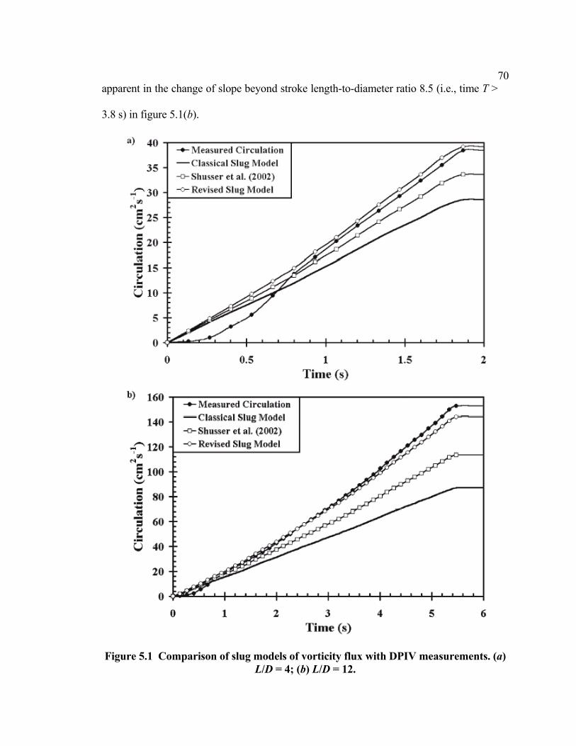
70 apparent in the change of slope beyond stroke length-to-diameter ratio 8.5 (i.e., time T >
3.8 s) in figure 5.1(b).
Figure 5.1 Comparison of slug models of vorticity flux with DPIV measurements. (a) L/D = 4; (b) L/D = 12.
71 The revised correction additionally affects the predicted non-dimensional
Norbury (1973) vortex core thickness ε of fully-formed vortex rings after pinch-off (Gharib
et al., 1998). Specifically, the revised correction shifts the curves in figure 10 of Shusser et
al. (2002) upward, so that the core thickness consistent with the vortex ring formation
number is reduced by 25 percent, to 0.3. This is in agreement with the experimental results
of Gharib et al. (1998).
5.3 Conclusions
An important correction to the slug model boundary layer correction proposed by
Shusser et al. (2002) has been discovered. The new result significantly improves agreement
with experimental measurements of starting jet vorticity flux and vortex ring core
thickness. The observed overestimation of vorticity flux by the revised correction at early
times is related to the dynamics of flow initiation, during which nozzle exit overpressure
has been observed to play an important role (Krueger and Gharib 2003). Nonetheless the
current result demonstrates the significant effect of boundary layer growth, especially for
the longer piston strokes needed to generate thick vortex rings.
5.4 Chapter References
Gharib, M., Rambod, E. and Shariff, K. 1998 A universal time scale for vortex ring
formation. J. Fluid Mech. 360, 121-140.
Krueger, P. S. and Gharib, M. 2003 The significance of vortex ring formation to the
impulse and thrust of a starting jet. Phys. Fluids 15, 1271-1281.
Norbury, J. 1973 A family of steady vortex rings. J. Fluid Mech. 57, 417-431.
Rosenhead, L. 1963 Laminar Boundary Layers. Clarendon Press.

72 Shariff, K. and Leonard, A. 1992 Vortex rings. Annu. Rev. Fluid Mech. 24, 235-279.
Shusser, M., Gharib, M., Rosenfeld, M. and Mohseni, K. 2002 On the effect of pipe
boundary layer growth on the formation of a laminar vortex ring generated by a
piston/cylinder arrangement. Theor. Comp. Fluid Dyn. 15, 303-316.
Willert, C. E. and Gharib, M. 1991 Digital particle image velocimetry. Exp. Fluids 10, 181-
193.

73
CHAPTER 6: Starting flow through nozzles with temporally variable exit
diameter
Submitted to Journal of Fluid Mechanics December 8, 2004
6.0 Chapter Abstract
Starting flow through a nozzle or orifice typically results in the transient formation
of a leading vortex ring and trailing jet. Experiments are conducted to investigate the
dynamics of this process in the case of a temporally variable nozzle exit diameter, with the
aim of understanding these flows as they occur in Nature and emerging technologies. By
kinematically decoupling the source flow from the nozzle motion, comparison across
several classes of exit diameter temporal variation is facilitated. Kinematic models of the
starting flows are used to accurately predict the fluid circulation produced by the vortex
generators and to emphasize the special role of the nozzle boundary layer in dictating the
nature of the global flow patterns. A dimensionless temporal parameter is derived in order
to track the vortex formation process for the various classes of nozzle motion. Dynamics of
vortex ring disconnection from the source flow are studied in this new dimensionless
framework. We show that temporally increasing the nozzle exit diameter as the starting
flow develops results in higher-energy vortex ring structures with peak vorticity located
further from the axis of symmetry relative to a static nozzle case. In addition, the
normalized energy supplied by the vortex generator is increased in this process. We do not
observe a delay in the onset of vortex ring disconnection from the trailing jet, as predicted
by previous numerical simulations. In contrast, growth of the leading vortex ring is
substantially augmented by temporally decreasing the nozzle exit diameter during fluid
74 ejection, as noted in a previous experiment. Normalized vortex ring circulation is
increased 35% in these cases, and the normalized energy of the generated vortex rings is
equivalent to that of Hill’s spherical vortex. These observed effects are explained by
considering the measured vorticity distribution and energy of the starting flows. Strategies
are suggested to exploit the discovered dynamics for various pulsed-jet applications.
6.1 Introduction
Pulsatile flows are among the most common and successful mechanisms for
convective fluid transport found in Nature. Although the selection of such techniques may
often be related to morphological constraints (Vogel, 1988, 1994), it remains noteworthy
that today we can observe the action of these unsteady flows in systems ranging from the
most primitive jellyfish locomotor to the complex trans-mitral and trans-aortic blood flows
in the animal heart.
Throughout the diverse catalogue of biological systems utilizing pulsatile flow, the
generated starting flow typically emerges from a nozzle or orifice with temporally variable
exit diameter. In systems with valve structures governing the flow, the observed motion of
the exit diameter is a necessary consequence of the transition from a closed valve to an
open one, and vice versa. An important example is the animal heart, where it has been
suggested that the interaction between the starting flows and the moving valves can be
correlated to some commonly observed cardiac pathologies (e.g., Gorman et al., 1996;
Yogonathan, Lemmon and Ellis, 2000; Handke et al., 2003).
In addition to the aforementioned use of starting flows for mass transfer, many
biological systems have co-opted pulsatile flow for locomotion. Certain cnidarians (e.g.,
jellyfish), cephalopods (e.g., squid), and bivalves (e.g., scallops) are most prominent in this

75 regard. Dabiri and Gharib (2003) measured exit diameter changes up to 30% during
steady swimming of Chrysaora fuscescens jellyfish. Transient exit diameter changes of
over 400% have been measured in the Lolliguncula brevis squid (Bartol, Patterson and
Mann, 2001), and the nozzle exit has been observed to close completely between fluid
pulses in the Loligo pealei squid (Anderson and DeMont, 2000). In many instances, the
temporal variation of the exit diameter is actively controlled, suggesting possible real-time
refinement of the fluid-structure interaction.
The fluid dynamical effect of a temporally variable nozzle exit diameter on a
starting flow has remained essentially unexplored. Our mandate for this study is at least
twofold. First, a better understanding of these systems can facilitate predictive models to
explain correlations between local fluid-structure interactions at the nozzle or orifice exit
and observed global features of the generated flow. Secondly, we may explain the physical
impetus for the specific programs of exit diameter temporal variation observed in Nature.
The design principles that are elucidated here may be transferable to emerging engineering
technologies, such as pulsed-jet propulsors and synthetic jets (see Glezer and Amitay, 2002
for a review).
From a kinematic perspective, the primary constituents of the starting flow through
a nozzle or orifice are a leading vortex ring and, in some cases, a trailing jet. A large
literature dealing with the dynamics of the quasi-steady jet is now available; however, our
understanding of the dynamics of the leading vortex ring is more limited. Gharib, Rambod
and Shariff (1998) experimentally identified a transition from formation of a single vortex
ring to generation of a leading vortex ring and trailing flow, as a function of the normalized
length of the ejected slug of fluid. Their work and subsequent models by Mohseni and

76 Gharib (1998), Linden and Turner (2001), and Mohseni (2001) have pointed to the effect
of an energetic requirement for the leading vortex ring during this transition, as stipulated
by the Kelvin-Benjamin variational principle (Kelvin, 1875; Benjamin, 1976). The
principle suggests that the leading vortex ring is incapable of further growth via ingestion
of fluid from the vortex generator if the energy of this source flow falls below the vortex
ring energy. Dynamical separation of the leading vortex ring from the trailing flow due to
this energetic effect is referred to as pinch-off in the literature.
Krueger (2001) and Krueger and Gharib (2003) attained the first measurements of
the dynamical effect of the vortex ring pinch-off process. They discovered that the time-
averaged force generated by a starting flow becomes maximal at the onset of vortex ring
pinch-off. This result suggests an optimal operating point just before vortex ring pinch-off
and also motivates the search for methods to delay vortex ring pinch-off altogether. Dabiri
and Gharib (2004a) successfully demonstrated the possibility of delaying vortex ring pinch-
off by imposing an external axisymmetric counter-flow during vortex ring formation.
Although those experiments demonstrated the feasibility of delaying vortex ring pinch-off
in general, it would be more useful to achieve similar results by manipulating properties of
the vortex ring generator itself, i.e., in the absence of external intervention.
Numerical studies by Rosenfeld, Rambod and Gharib (1998); Zhao, Frankel and
Mongean (2000); and Mohseni, Ran and Colonius (2001) have demonstrated that
parameters such as shear layer thickness, Reynolds number, and velocity profile can all
affect the dynamics of the pinch-off process. As this parameter space has only been
explored in silico, it is not immediately evident how each of these parameters should be
manipulated in practice. Notwithstanding, two practical methods have emerged from the

77 simulations of Mohseni et al. (2001) as potential candidates to delay pinch-off of the
leading vortex ring. In the first case, it is suggested to increase the velocity of the source
flow from the vortex generator to prolong feeding of dynamical invariants (i.e., energy,
impulse, and circulation) to the leading vortex ring. This concept is also proposed by
Shusser and Gharib (2000) as a corollary to their theory that vortex ring pinch-off occurs
when the velocity of the trailing jet (source flow) falls below the celerity of the leading
vortex ring.
The second method suggested by Mohseni et al. (2001) is to increase the radial
extent of the forcing (i.e., increase the nozzle or orifice exit diameter) as the starting flow
emerges from the vortex generator. In this way the shear layer of the source flow behind
the leading vortex ring could be moved away from the axis of symmetry, where it would
normally cancel with its mirror across the azimuthal plane of symmetry and lose strength.
These and other potential methods for pinch-off delay have not yet been validated
experimentally. Dr. J. J. Allen of New Mexico State University (2003, personal commu-
nication) has conducted experiments on vortex ring formation with a variable diameter
orifice aperture. Consistent with the prediction of Mohseni et al. (2001), preliminary results
indicated the effectiveness of an accelerating source flow for generating vortex rings of low
normalized energy, possibly indicative of delayed vortex ring pinch-off. In contrast,
increasing the radial extent of the forcing via a temporally increasing orifice aperture did
little to enhance the vortex ring formation process. Several questions remain unanswered
regarding the experimental method of Allen (2003), including the effects of fluid structures
generated on the upstream-facing side of the orifice plate (e.g., in stagnation zones);
aperture rotation about the axis of symmetry during orifice enlargement; and noncircular

78 aperture shape. Hence, we will only refer to those experiments in regard to the general
qualitative trends observed.
The objective of the present experiments is to study the dynamics of starting flows
through nozzles with temporally variable exit diameter. The nearly axisymmetric nozzle
used in these experiments serves as a generalization of the various nozzle and orifice
geometries observed in biological systems. Nozzle dynamics are decoupled from the source
flow by imposing a constant volume flux from a piston-cylinder apparatus at the inlet to the
nozzle during all experiments. This strategy proves to simplify the analysis and facilitate
quantitative comparison across all of the test cases. An important goal of these experiments
is to implement the strategies for pinch-off delay suggested by Mohseni et al. (2001) and
examined by Allen (2003). The observed starting flow dynamics are explained in terms of
the shear layer kinematics and leading vortex ring vorticity distribution and energy. In
addition, we examine relevant measures of pulsing performance to suggest benefits of
temporally variable nozzle and orifice exit diameters in biological systems and emerging
technologies.
The following section describes the apparatus and experimental methods in detail,
with special attention given to possible artifacts that could be introduced to the observed
fluid dynamics by the nature of the nozzle design. The results are catalogued in Section 3,
beginning with the kinematics of the nozzle boundary layer and shear layer efflux, and
subsequently focusing on the dynamics of the leading vortex ring. Nuances of dimensional
analysis for the time-dependent exit diameter are also presented in this section. Section 4
summarizes the analyses, provides comparison with previous numerical and experimental

79 observations of these flows, and discusses the physical basis for effective use of
temporally varying exit diameters in practice.
6.2 Apparatus and Experimental Methods
6.2.1 Apparatus design
Several challenges were faced in designing an apparatus to achieve temporal
variation of a nozzle exit diameter, without introducing undue complexity or unwanted
artifacts into the experiments. The design requirements included—but were not limited
to—distinct and repeatable separation of the nozzle boundary layer at a known radial
distance from the axis of symmetry and at a fixed axial location; a nozzle wall that is
sufficiently rigid to prevent deformation due to fluid forces, yet flexible enough to vary the
exit diameter over a large range; uniform radial actuation to maintain a nearly circular
shape at the nozzle exit plane; suppression of secondary vorticity generation by the
apparatus (e.g., as is present on the upstream-facing side of an orifice plate); and an
actuation mechanism that does not measurably disturb the flow.
This set of requirements is appropriately satisfied by the apparatus represented in
figure 6.1. The source flow is generated by a traditional piston-cylinder apparatus (cf.
Dabiri and Gharib, 2004c), with the inlet flow originating from the left hand side of the
hollow cylinder (inner diameter = 2.5 cm) in the schematic. A piston is oriented coaxially
with the hollow cylinder and has its diameter Dp flush with the inner surface of the
cylinder. The piston is driven by flow supplied from an external constant-head tank
operating at a total pressure head ∆p of 8.2 kPa. A computer-controlled solenoid valve
meters the flow using an impulsive velocity profile with a rise time of approximately 300

80 ms to steady flow at 8.8 cm3s-1. Flow rates are monitored by an ultrasonic flow probe at
the inlet to the cylinder and are recorded to a computer hard disk via a LabVIEW program.
A single value of the constant volume flux is used throughout all of the experiments
described in this paper. In this way, the source flow merely serves as a control parameter
and falls out of much of the subsequent analyses. Source flow from the piston-cylinder
apparatus enters the nozzle inlet, which is mounted immediately downstream.
The nozzle is constructed from a 5.1 cm length of originally straight latex rubber
tubing with 1.5 cm nominal inner diameter, 0.08 cm nominal thickness, and sharp edges.
Optimal wall thickness was determined from repeated iterations of the design to facilitate
maximum actuation of the exit diameter without becoming susceptible to deformation due
to fluid forces. The nozzle inlet diameter is matched to the inner diameter of the upstream
hollow cylinder by fitting the elastic tube over the outer diameter of the cylinder lip (Do =
3.1 cm). To facilitate a smooth transition from the cylinder to the nozzle, the cylinder lip is
sharpened to form a 7 degree wedge from its outer diameter to inner diameter (cf. figure 1
of Dabiri and Gharib, 2004c). The nozzle is held to the cylinder by elastic forces induced
during the process of stretching the latex tube over the cylinder lip, and by a series of
compression clamps placed around the cylinder outer diameter.
For simplicity in later analyses, a spatially linear contraction in nozzle diameter
from the inlet to the exit plane is desired. This is accomplished by supporting the elastic
nozzle with 16 straight stainless steel cotter pin support spars equally spaced azimuthally
around the nozzle. Each support spar has a hairpin shape and is fitted over the downstream
edge of the elastic nozzle with both prongs extending upstream along the length of the
nozzle. The junction of the two prongs of each hairpin is positioned at the nozzle exit plane.

81 The free ends of the two prongs of each hairpin are fixed to the inner and outer surfaces
of the nozzle, respectively, using a waterproof adhesive. These free hairpin ends effectively
act as a pin joint when the nozzle is actuated.
A water-resistant actuating cable is connected to the hairpin junction of each
support spar at the nozzle exit plane; the cable extends radially to a perforated conical shell
that acts as a fixed pulley. The apex of the cone is truncated, and the piston-cylinder
apparatus is mounted rigidly through the apical opening. After passing through a hole in the
wall of the conical fixed pulley, the cable is turned 90 degrees toward an axial orientation
upstream, where its terminal end is mounted to the inner surface of a hollow drum. The
drum is mounted coaxially to the piston-cylinder apparatus on a roller bearing, so that it is
free to rotate about the axis of symmetry.
When the drum rotates, the terminal end of the cable that is mounted to the drum
moves azimuthally. Since the cable is inextensible, the other end of the cable connected to
the support spar is pulled radially toward its respective hole in the conical pulley. By this
mechanism, a single degree of freedom in the rotating drum is transduced to radial
actuation at 16 uniformly spaced locations around the azimuth of the nozzle exit plane.
A flat belt pulley system connects the drum to a computer-controlled stepper motor
that governs the nozzle motion. The drum rotation necessary for actuation of the nozzle
from minimum to maximum diameter is approximately 30 degrees. Details of the specific
programs of exit diameter variation used in these experiments will be presented in a
subsequent section.

82 The entire piston-cylinder-nozzle apparatus is submerged in a 60 cm H × 40 cm
W × 100 cm L water tank with transparent walls. Mounting points are located along the
cylinder and around the azimuth of the conical pulley.

83
Figure 6.1 Apparatus for temporal variation of nozzle exit diameter. (a) schematic.
(b) laboratory image. (c) front view of nozzle exit plane.

84 6.2.2 Effects of noncircular nozzle shape
Although most of the design requirements are satisfied ipso facto the apparatus
described above, an important concern must be directly addressed regarding the shape of
the nozzle exit. Figure 6.1(c) shows the front view of the nozzle at the exit plane, in
proportions that are approximately to scale. The cotter pin support spars, with dimensions
of 0.13 cm azimuthally and 0.08 cm per prong radially, act as a finite amplitude disturbance
with wavenumber 16 on the starting flow. It is reasonable to question the behavior of this
disturbance in time, especially as it relates to the forming leading vortex ring.
The stability theory for an exact representation of this flow is unresolved and also
beyond the scope of this paper. However, we can appeal to the classical inviscid theory and
make use of qualitative experiments to develop a convincing argument for the negligible
effect of the nozzle shape perturbations on the flow.
Azimuthal wave development on vortex rings has been appreciated for decades, be-
ginning with the experimental work of Krutzsch (1939). The physics of the phenomenon
were elucidated by Widnall, Bliss, and Tsai (1974) and further refined by Widnall and Tsai
(1977), Saffman (1978), and Shariff, Verzicco, and Orlandi (1994). The work of Saffman
(1978) is especially useful in the present context, as it examines the dependence of the most
unstable wavenumber on the Reynolds number (based on ring celerity and nozzle exit
diameter) and diameter-normalized length of the ejected slug of fluid T*. Combining
equations (4.4) and (4.6) of his paper leads to a relationship between the most unstable
wavenumber, the critical Reynolds number, and the parameter T*. The equations predict
that the growth of azimuthal disturbances of large wavenumber is suppressed at low
Reynolds numbers. For the normalized fluid slug length in the vortex rings studied here (T*

85 ≤ 8), the Reynolds number corresponding to an unstable wavenumber 16 (i.e., Re ≈ 6 ×
104) is approximately two orders of magnitude higher than the conditions of the present
experiments.
We are quick to note that this is a simplified calculation. To further support the
above conclusion, we conducted dye visualization experiments of the starting jet formed by
the apparatus at the minimum and maximum nozzle exit diameter. In both cases the vortex
ring remained laminar and did not retain visible signs of the shape perturbation at the
nozzle exit (at wavenumber 16 or otherwise) throughout observation of the rings until the
dye began to dissipate far downstream. Especially in light of the fact that our observations
will focus on the near-field flow, we proceed under the assumption that the measured
dynamics do not represent artifacts from non-idealities in the experimental apparatus. The
nozzle exit diameter in each case is defined based on an equivalent circle with cross-
sectional area equal to the measured nozzle exit area.
6.2.3 Quantitative flow visualization
Kinematics of the flow field are measured using digital particle image velocimetry
(DPIV, cf. Willert and Gharib, 1991; Adrian, 1991). The hardware and parameters of the
technique are essentially the same as described in Dabiri and Gharib (2004c). A laser sheet
from a Nd:YAG laser source illuminates a plane of symmetry relative to the vortex
generator, providing an azimuthal view of the axisymmetric starting flow from an
orthogonallyoriented digital CCD camera at 30 Hz. In the present experiments the flow
field measures 7.8 cm (3.1 Dp) radially from the axis of symmetry and from 0.77 cm (0.3
Dp) to 15.8 cm (6.2 Dp) downstream. The field is imaged at a resolution of approximately
65 pixels per cm, sufficient to resolve the vorticity distribution in the vortex ring core.

86 Timing of source flow initiation, nozzle actuation, laser firing, and image capture
is coordinated by an in-house code and LabVIEW data acquisition hardware. Velocity and
vorticity measurements possess an uncertainty of 1 percent and 3 percent, respectively.
6.2.4 Experimental parameter space
The extreme positions of the nozzle exit diameter are plotted to approximate scale
in figure 6.1(c). The maximum nozzle exit area is nearly 200 percent of the minimum exit
area. These positions are the end points of the temporal exit diameter variation in each of
the experiments conducted. Figure 6.2 plots the specific programs of nozzle exit diameter
variation studied in these experiments. The diameter profiles were measured from frontal
view video recordings of the nozzle undergoing each actuation program. The measured
diameter at each instant is an effective value computed as De = 2(Ae/π)1/2, where Ae is the
nozzle exit area. This method accounts for the reduced nozzle exit area due to the presence
of cotter pin support spars at the exit plane (figure 6.1c) and is the source of the lower
minimum exit diameter (i.e., De = 1.21 cm) relative to the nominal pre-installation tube
diameter (i.e., De = 1.5 cm). Static nozzle cases at minimum (De = 1.21 cm = 0.48 Dp;
henceforth SMIN) and maximum (De = 1.69 cm = 0.67 Dp; henceforth SMAX) diameter
are included as control sets. The dynamic nozzle cases consist of a slower-opening (SO)
case, a faster-opening (FO) case, a slower-closing (SC) case, and a faster-closing (FC) case.
The time derivative of the nozzle exit diameter change is shown in figure 6.3. These
plots indicate that the peak temporal variation in the faster cases is double that of the slower
cases. The slight modulation in nozzle exit diameter rate of change for the SO and FO cases
(at time t = 1.2 s and 0.6 s, respectively) occurred due to artifacts related to elastic

87 deformation of the nozzle by the support spars, but did not measurably affect the
observed vortex dynamics. Dynamic nozzle programs are repeatable to within 3%.
Figure 6.2 Programs of nozzle exit diameter temporal variation.
Figure 6.3 Rate of diameter change for each program of nozzle exit diameter
temporal variation.

88 Nozzle contraction angle varies between 12 degrees when the exit diameter is
in its maximum position, and 18 degrees when in its minimum position.
φ
The Reynolds numbers at which these experiments were conducted range between
660 and 920 based on the nozzle exit velocity and diameter, and between 1500 and 3500
based on the circulation of the leading vortex ring. These Reynolds numbers are consistent
with several of the biological systems discussed in the Introduction, such as jellyfish
(Daniel, 1983; Dabiri and Gharib, 2003) and juvenile squid (Bartol et al., 2001), but are
below the range of some higher-speed jetters such as adult squid (Anderson and DeMont,
2000). Given that Gharib et al. (1998) have demonstrated the process of vortex ring
formation in starting jets to be robust up to at least a Reynolds number of 6000 (based on
the circulation of the leading vortex ring), the present results should be applicable to many
of the higher-speed flows as well.
Measurement results are presented herein typically using single representative data
sets for each nozzle program (figure 6.6 is a notable exception). Three or more iterations
were conducted for each program of nozzle exit diameter temporal variation to ensure that
stated values accurately represent each test case. The maximum uncertainty in each
representative data set is ±5%.
6.2.5 Boundary layer dynamics
Didden (1979) clearly demonstrated the special role of boundary layer dynamics in
the development of starting flows, especially in relation to leading vortex ring formation.
Using laser Doppler velocimetry (LDV) measurements, he observed quantitatively how the
motion of the boundary layer at flow initiation dominates the roll-up of the leading vortex
ring. In addition, boundary layer growth within the hollow cylinder of the vortex generator

89 was shown to lead to an increase in vorticity flux into the starting jet. These interesting
aspects of starting flows cannot be captured by a simplified slug model of the flow, which
neglects boundary layer effects altogether (cf. Shariff and Leonard, 1992; Krueger and
Gharib, 2003).
Shusser et al. (2002) suggested incorporating a Rayleigh-Stokes solution to account
for boundary layer growth within the hollow cylinder of a piston-cylinder vortex generator.
A modified version of their solution, presented by Dabiri and Gharib (2004b), achieved
close agreement with DPIV measurements of the generated vorticity flux.
In the present apparatus, we must address the added complexity of a spatially and
temporally accelerating mean flow due to the presence of a nozzle with temporally variable
contraction ratio Dp/De downstream of the piston-cylinder apparatus. The effect of this
unsteady flow on the boundary layer that formed upstream in the piston-cylinder apparatus
will largely dictate the nature of the starting flow that emerges from the nozzle exit.
A quasi-steady analysis predicts that the boundary layer entering the nozzle from
the piston-cylinder apparatus will become thinner due to the nozzle contraction, perhaps
eliminating the need for the correction of Dabiri and Gharib (2004b) to the starting flow.
However, the combination of spatial and temporal accelerations in the real starting flow
adds complexity that cannot be easily captured by a quasi-steady analysis.
Our piston-cylinder flow rate data and nozzle exit velocity profile measurements
obtained using DPIV are sufficient to determine the level of boundary layer thinning
achieved in each of the experiments performed here. This information will be critical for
properly modeling these starting flows, especially in predicting the vorticity flux from the
nozzle in each experiment.

90 Measurements of the exit velocity profile for each temporal pattern of nozzle
diameter variation indicate that those cases with larger average nozzle contraction ratio
during initiation of the starting jet (i.e., SMIN, SO, and FO cases) exhibit significantly less
boundary layer thinning than those with smaller average nozzle contraction ratio over the
same period of time (i.e., SMAX, SC, and FC cases). Figure 6.4 exemplifies these trends
for the SMIN and SMAX diameter cases. Initially the boundary layer dynamics are similar
in the two cases (figure 6.4a). However, at later times the larger nozzle contraction ratio in
the SMIN case causes boundary layer vorticity from the upstream piston-cylinder apparatus
to be convected downstream out of the nozzle faster than it is rearranged by diffusion,
allowing the upstream velocity profile (i.e., at the nozzle entrance) to pass through the
nozzle essentially unchanged. Thus, the velocity profile in the SMIN case does not exhibit
thinning similar to that expected in a quasi-steady flow. By contrast, the SMAX case has a
smaller nozzle contraction ratio and therefore a lower spatial acceleration in the nozzle.
Accordingly, upstream vorticity from the piston-cylinder apparatus persists in the nozzle
for a longer duration, allowing viscous diffusion to rearrange the boundary layer. In these
cases boundary layer thinning is more substantial (figure 6.4b).
The observed dynamics of the boundary layers in these starting flows are a
consequence of the specific experimental apparatus implemented for vortex generation.
There exist various methods to mitigate the effect of the boundary layer so that it does not
play such a large role in the fluid dynamics (e.g., Joslin, 1998). Our strategy is to embrace
the nonessential boundary layer effects in order to better understand these starting flows in
general, and to better relate to biological systems, most of which appear to lack immediate
methods for boundary layer elimination.

91
Figure 6.4 Velocity profile of fluid efflux at X = 0.3 Dp for static minimum and maximum diameter cases. (a) T = 0.67 s. (b) T = 2.0 s. Y* is the radial coordinate
normalized by the location at which U/Umax = 0.5.
92 In the following sections we will model the starting flow for the SMAX, SC, and
FC nozzles as if the piston-cylinder boundary layer has completely thinned in the nozzle,
while modeling the SMIN, SO, and FO cases as if the piston-cylinder boundary layer has
passed through the nozzle unchanged. We do recognize that boundary layer thinning will
occur to some degree in every test case. However we will show that this approximation is
sufficient to generate a realistic picture of the starting flows in these experiments.
6.3 Results
6.3.1 Vorticity flux
The flux of vorticity from the starting flow boundary layer provides a useful
measure of the dynamical contribution of the vortex generator to the ambient fluid.
Measuring the flux of vorticity in practice typically requires a precise velocimeter, a
prospect that is often inconvenient when studying biological systems or engineering
technologies with auxiliary components that interfere with controlled experimental
observations. It is therefore desirable to develop analytical models to accurately predict the
vorticity flux from starting flows, based on known parameters of the vortex generator.
Naturally, our focus is directed toward starting flows through temporally variable nozzles.
In the case of a piston-cylinder apparatus, the classical slug model result for the
vorticity flux is
( ) ( )tUtt p
2
slug 21
dd
≈Γ , (6.3.1)
where Γ is the circulation delivered by the vortex generator, and Up is the (possibly time-
dependent) piston speed.

93 By replacing the piston velocity with the fluid volume flux and the circular
nozzle or orifice exit diameter D
Ω&
e, we arrive at a generalized vorticity flux model for an
arbitrary source flow with circular nozzle or orifice exit:
( ) ( )( )tDtt
t e42
2
slug
8dd
πΩΓ &
≈ . (6.3.2)
Boundary layer growth inside the vortex generator results in a decreased flow
velocity near the walls and concomitant increase in velocity outside the boundary layer in
order to satisfy continuity. As mentioned in the previous section, only a simplified model of
this process is tractable in the present context. Using the result of Dabiri and Gharib
(2004b), the vorticity flux in this case is predicted by
( ) ( )( )
( )( )
2
21
21
42
2
BLG
818dd
+≈
tDt
tDtt
t ee πν
πΩΓ &
. (6.3.3)
According to the conclusions of the preceding section, (6.3.2) was used to predict
the vorticity flux in the SMAX, SC, and FC cases, while (6.3.3) was applied to the SMIN,
SO, and FC cases. The results are plotted in figure 6.5. After initial vortex ring roll-up, the
agreement is very good in each case, especially considering that no empirical scaling fac-
tors have been used. Discrepancies shortly after flow initiation at time T = 0 are due to
difficulties in measuring the flow field close to the nozzle exit, and due to vortex ring roll-
up and overpressure effects previously documented by Didden (1979) and Krueger (2001),
which cannot be captured by these models. The former issue, which causes an uncertainty
in the measured time of flow initiation, will be revisited in the following section. Notably,
the global flow—represented by the total generated circulation—is accurately predicted by
the models.

94
Figure 6.5 Measured and predicted circulation generated for each program of nozzle
exit diameter temporal variation. (a) SMIN, SO, and FO cases. (b) SMAX, SC, and FC cases.

95 6.3.2 Dimensional analysis
In preparation for the ensuing discourse on leading vortex ring dynamics, it is
useful to prepare a dimensionless framework in which to present the results. Gharib et al.
(1998) define a vortex ring formation time corresponding to the dimensionless length of the
fluid slug ejected from a piston-cylinder apparatus:
p
p
DtU
T ≡*GRS , (6.3.4)
where the overbar denotes a running time average. Mohseni et al. (2001) use a modified
form of this definition, in which the piston speed is replaced by the vortex ring celerity.
The difficulty with these definitions in a general starting flow is that the former is
valid strictly for a constant-diameter vortex generator, and the latter requires knowledge of
the motion of the leading vortex ring, which may be inaccessible or even irrelevant to the
particular flow of interest.
A generalized dynamic dimensionless time scale based on the parameters of the
vortex generator can be derived by considering an infinitesimal increment in the formation
time of Gharib et al. (1998):
( )( ) ttDtU
Te
e dd * = . (6.3.5)
In (6.3.5), the nozzle exit velocity Ue (i.e., the free-stream flow velocity outside the
boundary layer as in Dabiri and Gharib 2004b) is used as the appropriate characteristic
velocity instead of the piston speed. Integrating over the duration of fluid ejection, we
arrive at a dimensionless time scale that properly accounts for temporal changes in the exit
diameter:

96
( )( ) t
DU
DU
Te
et
e
e
== ∫0
* dτττ
. (5.3.6)
This new dimensionless parameter is monotonically increasing for any temporal
variation of the exit diameter, as it must be to accurately reflect the irreversible nature of
the fluid ejection process. In contrast, definition (5.3.4) of Gharib et al. (1998) gives a
spurious result of decreasing formation time when the instantaneous or time-averaged exit
diameter is increasing.
Consistent with the preceding result, the circulation is properly normalized using
the terms ( )ee DU and 2eU as
( )
2
*
e
ee
U
DUΓΓ = . (5.3.7)
Despite the inclusion of a boundary layer correction to the exit velocity in the
SMIN, SO, and FO cases, a plot of normalized circulation versus formation time should
still possess a slope of 1/2 in accord with the slug model equation (6.3.1). The slope is pre-
served because the boundary layer correction appears in both the circulation and time
normalizations, leaving their ratio unaffected. Figure 6.6 shows the circulation trends from
several iterations of each nozzle case. The data are shifted along the abscissa so that the
linear portion of each trend has its intercept at the origin. After initial scatter, all of the data
collapses to the reference line with slope equal to 1/2.
Data scatter at early formation time is largely due to differences in the manner in
which the leading vortex ring enters the DPIV measurement window from the upstream
boundary at X = 0.3Dp. The trend of increasing measured circulation during this time is
dominated by propagation of the vortex ring core vorticity into the measurement window at

97 the upstream boundary. Hence, the measured data trends at early formation time are not
necessarily indicative of the actual rate of vorticity generation by the starting flow. This
effect has been previously observed by Didden (1979) using LDV measurements and
Dabiri and Gharib (2004b) using DPIV. Since this effect occurs well before vortex ring
pinch-off, it is an artifact with little influence on the measurements of importance to these
experiments. Nonetheless, we can quantitatively bound this effect by assuming that the
vortex cores possess a Gaussian vorticity distribution and enter the measurement window
in a quasi-steady fashion. The fluid circulation entering the measurement window due to
this motion will then be an error function of time by definition, since the circulation
measurement is the definite integral of an assumed normal distribution of vorticity
(centered at the vortex core) over the finite spatial region 0.3Dp ≤ X ≤ 6.2Dp. Figure 6.6
indicates one such curve that effectively bounds the scatter in these experiments.
Figure 6.6 Normalized circulation versus formation time for each program of nozzle exit diameter temporal variation. Solid lines indicate slope = 1/2 and error function
bound.

98 As an aside, the reader may be tempted to correlate the observed intersection of
the linear and error function curves in figure 6.6 to the fact that pinch-off typically occurs at
this same location in the space of normalized circulation versus formation time (i.e., [T*,
Γ*] = [4, 2]). We strongly suggest that this is merely a coincidence in the present case. This
conclusion is supported by the fact that, as previously mentioned, the data has been
artificially shifted in formation time to force the linear trends to intersect the origin. In
addition, the error function curve chosen to represent the lower bound of data scatter will
change depending on the location of the upstream boundary of the measurement window.
These choices are completely independent of the dynamics of leading vortex ring pinch-off.
6.3.3 Leading vortex ring pinch-off and vorticity distribution
With a dimensionless perspective on the fluid dynamics in place, we are prepared to
examine the physics of leading vortex ring pinch-off. To reiterate, our focus on the pinch-
off process is motivated by its dynamical significance as discovered by Krueger (2001),
and the possibility of generating vortex rings of low dimensionless energy as implied by
the results of Mohseni et al. (2001).
The method of Gharib et al. (1998) is used to determine the dimensionless vortex
formation time corresponding to the onset of pinch-off, i.e., the formation number F. By
measuring the circulation of the leading vortex ring after pinch-off, the formation time at
which this circulation was generated by the starting flow is found. Figure 6.7 plots the
dimensionless circulation versus formation time for the SMIN, SO, and FO nozzle cases.
The formation time at the onset of pinch-off consistently falls between 3.7 and 4.4 for each
group. These data are in agreement with the range observed by Gharib et al. (1998).

99 Contrary to the prediction of Mohseni et al. (2001), we do not observe a significant delay
in vortex ring pinch-off for the cases with temporally increasing nozzle exit diameter.
Our finding is consistent with the results of Allen (2003), who also did not observe
a beneficial effect of a temporally increasing exit diameter on vortex ring formation.
Further examination of the leading vortex ring vorticity profile for each case provides the
insight necessary to understand why the method has been ineffective. Figure 6.8 plots the
vorticity profile along a radial section of the leading vortex ring at the formation number.
For the SMIN case, the core vorticity distribution is qualitatively similar to a Gaussian-type
profile. When the nozzle exit diameter is increased temporally as the starting flow emerges,
the locations of peak core vorticity and the core vorticity centroid are both moved radially
away from the axis of symmetry, as Mohseni et al. (2001) predicted. Furthermore, the
radial motions of the vorticity peak and centroid occur nearly in direct proportion to the
radial motion of the nozzle exit diameter.
However, in each case the portions of the shear layer closer to the axis of symmetry
are unaffected by the nozzle motion; the near-axis vorticity consistently extends to the
symmetry axis at the same formation time as the static nozzle case. We can conclude that
although the temporal increase in nozzle exit diameter was effective in manipulating the
radial location of peak vorticity in the core, the nozzle motion was insufficient to prevent
the entire shear layer from encroaching on the axis of symmetry. Movement of the entire
shear layer away from the centerline is necessary to delay vortex ring pinch-off.
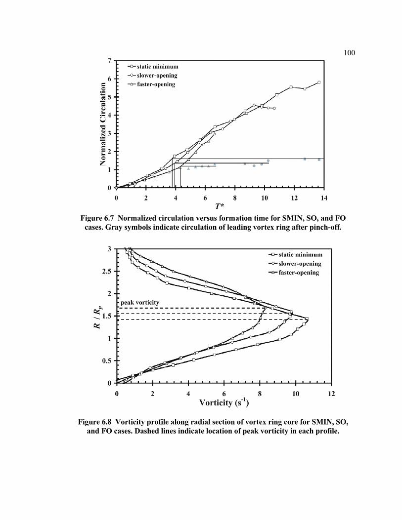
100
Figure 6.7 Normalized circulation versus formation time for SMIN, SO, and FO
cases. Gray symbols indicate circulation of leading vortex ring after pinch-off.
Figure 6.8 Vorticity profile along radial section of vortex ring core for SMIN, SO, and FO cases. Dashed lines indicate location of peak vorticity in each profile.

101 The present results may be attributed in part to the thickness of the shear layer
at the relatively low Reynolds numbers of these experiments. We remain open to the
possibility that at much higher Reynolds numbers, the shear layer might be sufficiently thin
that it uniformly follows the motion of the vorticity peak. A more general discussion of
dynamical benefits of the temporally increasing nozzle exit diameter is reserved for the
concluding section of this chapter.
Circulation data for the SMAX, SC, and FC nozzle cases is shown in figure 6.9. In
the absence of nozzle motion (i.e., SMAX case), leading vortex ring pinch-off occurs at a
maximum formation number of 4.6. This is reasonably consistent with the range reported
by Gharib et al. (1998). When a temporally decreasing nozzle exit diameter is introduced,
the formation number increases substantially, to 6.9 for the SC case and to 8.0 for the FC
case. This delay in vortex ring pinch-off is dramatically greater than that achieved by
Dabiri and Gharib (2004a) using an external bulk counter-flow. Normalized circulation of
the leading vortex ring is also increased by up to 35% over the static nozzle case.
For consistency with the preceding analysis, we plot the vorticity distribution along
a radial section of the vortex ring core for the SMAX, SC, and FC cases at the formation
number (figure 6.10). Unlike the trend observed for the radially-increasing exit diameter,
the radially-decreasing exit diameter has little effect on the location of peak vorticity or the
core vorticity centroid. There is, however, a large change in the magnitude of peak
vorticity. The FC nozzle case exhibits peak vorticity at nearly double the peak level of the
static nozzle. In addition, the temporally decreasing exit diameter nozzle cases possess a
distinct discontinuity in the slope of the vorticity distribution approximately 1R/Rp from the
axis of symmetry.

102 The vortex dynamics leading to these observed pinch-off and vorticity
distribution trends are best explained in the context of a discourse on the leading vortex
ring energy, as follows.
Figure 6.9 Normalized circulation versus formation time for SMAX, SC, and FC
cases. Gray symbols indicate circulation of leading vortex ring after pinch-off.
Figure 6.10 Vorticity profile along radial section of vortex ring core for SMAX, SC, and FC cases. Dashed line indicates approximate location of peak vorticity in each
profile.

103 6.3.4 Leading vortex ring energy
The dimensionless vortex ring energy E* is an especially useful parameter for
investigating the dynamics of these starting flows, as it invokes the dynamical invariants
being delivered from the vortex generator. Measuring the vortex ring energy is difficult in
practice because it requires powers, quotients, and integrals of the velocity and vorticity
fields:
[ ] [ ] 232122321*
dddd
dd
∫∫∫==
rxrxr
rx
IEE
ωωπ
ωψπ
Γ, (6.3.8)
where E, I, and Γ are the dimensional energy, impulse, and circulation, respectively, and ψ
is the streamfunction. The velocity and vorticity fields have been measured with nonzero
error, which will subsequently compound when computing the dimensionless energy. An
additional source of uncertainty arises in selection of the vorticity contour that will be used
to define the vortex core. Definitions of the vortex core based on a given vorticity contour
level are ad hoc and make comparison between different cases somewhat tenuous.
A reliable method of obtaining the leading vortex ring energy is indicated in the
work of Gharib et al. (1998). As dictated by the Kelvin-Benjamin variational principle, we
can exploit the fact that the leading vortex ring energy is equal to the instantaneous energy
of source flow delivered by the vortex generator at the formation number.
Using this strategy, we first revisit the pinch-off results for nozzle cases with
temporally increasing exit diameter. Figure 6.11(a) plots the dimensionless energy supplied
by the vortex generator in the SMIN, SO, and FO cases (using the exit velocity Ue(t) to
compute source flow impulse and energy), along with the leading vortex ring energy. For
the SMIN case, the dimensionless energy of the leading vortex ring is 0.40. This value is

104 higher than that found by Gharib et al. (1998) but in the range of Mohseni et al. (2001)
for vortex rings with similar normalized circulation. Movement of the peak vorticity away
from the axis of symmetry by the nozzle motion results in vortex ring vorticity distributions
with larger normalized energy, over 0.5 for the FO nozzle.
It is interesting to note that the nozzles with temporally increasing exit diameter
successfully deliver source flow at higher dimensionless energy than the static nozzle case.
Gharib et al. (1998) predict that this condition of increased dimensionless energy from the
vortex generator is necessary in order to achieve a delay in pinch-off of the leading vortex
ring. However, in the present experiments the concomitant increase in leading vortex ring
energy due to vorticity redistribution (viz. radial movement of the core vorticity peak and
centroid) negates any potential benefit from the increased energy source. If the source flow
could be delivered at the same elevated energy level without affecting the leading vortex
ring vorticity distribution, a substantial delay in vortex ring pinch-off might be achieved.
The dynamics of the SC and FC cases are more complex. In these nozzle cases, we
observed substantial increases in the formation number and the normalized circulation of
the leading vortex ring. One of two effects (or perhaps a combination thereof) can be
expected to play a role in the augmented starting flow dynamics. In the first case, one might
suspect that the increasing source flow velocity enables delay of leading vortex ring pinch-
off, as predicted by Shusser and Gharib (2000) and Mohseni et al. (2001). Alternatively,
the nozzle motion may have induced a change in the distribution of vortex ring vorticity,
resulting in a lower dimensionless energy of the leading vortex ring and an associated
decrease in the required source flow energy to sustain ring growth.

105
Figure 6.11 Normalized vortex generator energy versus formation time. Circled
points in each plot indicate leading vortex ring energy. (a) SMIN, SO and FO cases. (b) SMAX, SC and FC cases.
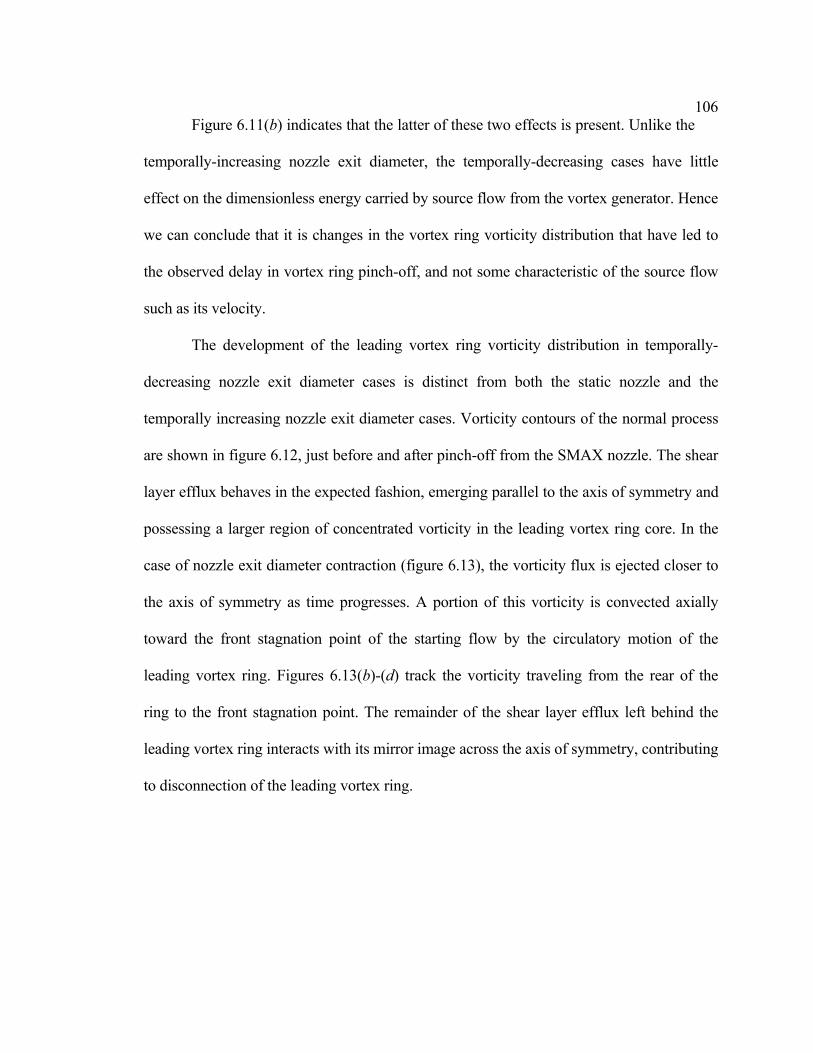
106 Figure 6.11(b) indicates that the latter of these two effects is present. Unlike the
temporally-increasing nozzle exit diameter, the temporally-decreasing cases have little
effect on the dimensionless energy carried by source flow from the vortex generator. Hence
we can conclude that it is changes in the vortex ring vorticity distribution that have led to
the observed delay in vortex ring pinch-off, and not some characteristic of the source flow
such as its velocity.
The development of the leading vortex ring vorticity distribution in temporally-
decreasing nozzle exit diameter cases is distinct from both the static nozzle and the
temporally increasing nozzle exit diameter cases. Vorticity contours of the normal process
are shown in figure 6.12, just before and after pinch-off from the SMAX nozzle. The shear
layer efflux behaves in the expected fashion, emerging parallel to the axis of symmetry and
possessing a larger region of concentrated vorticity in the leading vortex ring core. In the
case of nozzle exit diameter contraction (figure 6.13), the vorticity flux is ejected closer to
the axis of symmetry as time progresses. A portion of this vorticity is convected axially
toward the front stagnation point of the starting flow by the circulatory motion of the
leading vortex ring. Figures 6.13(b)-(d) track the vorticity traveling from the rear of the
ring to the front stagnation point. The remainder of the shear layer efflux left behind the
leading vortex ring interacts with its mirror image across the axis of symmetry, contributing
to disconnection of the leading vortex ring.

107
Figure 6.12 Vorticity contours of the flow downstream of the static maximum
diameter nozzle. Flow is from left to right. Solid and dashed lines indicate positive and negative vorticity, respectively. Contour spacing is 2 s-1.
Figure 6.13 Vorticity contours of the flow downstream of the FC diameter nozzle.
Flow is from left to right. Solid and dashed lines indicate positive and negative vorticity, respectively. Contour spacing is 3 s-1. Downstream convection of vorticity along the axis of symmetry is tracked by a cross symbol placed at the local vorticity
peak.

108 Crescent-shaped vorticity patches arise in the leading vortex ring after this
process (e.g., figure 6.13d), in contrast with the typical elliptic patches. In the preceding
section, the vorticity distribution near the axis of symmetry was noted to display a trend
different from the typical Gaussian profile. From figure 6.13 we can now see that this effect
is due to the shear layer vorticity that was fed close to the axis of symmetry and
subsequently passed from the rear of the ring to the front stagnation point. The motion of
this vorticity also appears to have prevented the leading vortex ring cores from following
the nozzle wall motion toward the axis of symmetry, as was observed (in the opposite
sense) in the temporally-increasing nozzles. This explains the difference in the dynamics of
the vorticity peaks plotted in figures 6.8 and 6.10.
Vortex rings with very low dimensionless energy are generated by the process
described above. Starting flow through the FC nozzle formed leading vortex rings with
dimensionless energy equal to 0.165 ± 0.009. This value agrees with direct measurements
using equation (6.3.8), which gave values in the range of 0.16 ± 0.02. For comparison,
Hill’s spherical vortex has a dimensionless energy of 0.160. The vortex rings generated in
the present experiments are not Hill’s vortices, however, because the vorticity distribution
is not uniformly linear in the radial direction. Furthermore, the rings could potentially have
dimensionless energy lower than that of Hill’s vortex, as demonstrated by Mohseni et al.
(2001) for vortex rings formed at low Reynolds numbers (i.e., less than 1000 based on the
leading vortex ring circulation). Nonetheless, the comparison with Hill’s vortex is
noteworthy because previous analytical studies of the pinch-off process have invoked the
Norbury family of vortices, which includes Hill’s vortex as its limiting member (e.g.,
Gharib et al., 1998; Mohseni et al. 2001; Linden and Turner, 2001). In particular Linden

109 and Turner (2001) predict that vortex rings with dimensionless energy equal to Hill’s
vortex can be achieved by a constant-diameter piston-cylinder apparatus if pinch-off is
delayed until a dimensionless vortex formation time of 7.83. That predicted pinch-off time
is very close to the values observed here for vortex rings with Hill-type dimensionless
energy formed by the FC nozzle.
6.3.5 Leading vortex ring fluid transport
Finally, we present an aspect of starting flow dynamics that is largely absent from
the literature; namely, the issue of how much fluid is transported by the leading vortex ring
of the starting flow. Although the preceding sections have identified effective means to
delay pinch-off and produce vortex rings with low dimensionless energy and high
normalized circulation, we must ask if there is any penalty being paid in the process of
mass transfer relative to the static nozzle cases. Since the volume flux through each nozzle
is identical, such a comparison can be made given the available data.
Figure 6.14 plots the volume of source flow carried in the leading vortex ring of
each starting flow through a temporally variable nozzle exit diameter, Ω(t), relative to its
static nozzle counterpart at pinch-off Ω0. Temporal increases in the nozzle exit diameter
have a minor effect on the volume of fluid transported by the leading vortex ring. In
contrast, the temporally decreasing nozzle exit cases deliver only 80% of the fluid that the
static nozzle is capable of transporting via the leading vortex ring. The practical
significance of this performance limit will depend on the details of a particular application,
especially the expense of reciprocating the motion to generate additional vortex rings.
Nonetheless this result clearly demonstrates the need to examine starting flow performance
from several perspectives, both dimensional and independent of physical units.

110 Table 1 summarizes relevant dimensional parameters of the leading vortex rings
measured in each test case. This data complements the dimensionless perspective
commonly taken to study the dynamics of vortex ring pinch-off.
Figure 6.14 Delivered fluid fraction for leading vortex rings in nozzle cases with
temporally variable exit diameter.
Nozzle Program
Formation Number
Pinch-off Time
Vortex Circulation
Vortex Diameter
SMIN 3.7 0.57 s 17.5 cm2s-1 3.6 cm
SO 3.9 0.53 14.5 4.1
FO 4.3 0.60 13.4 4.3
SMAX 4.6 1.95 17.9 4.4
SC 6.9 1.56 30.2 4.8
FC 8.0 1.54 32.8 4.5
Table 6.1 Dimensional parameters of the leading vortex ring for each nozzle program. Values are representative and possess a maximum uncertainty of ±5%.
111 6.4 Summary and Conclusions
This chapter has described a detailed experimental study of starting flow through
nozzles with temporally variable exit diameter. Our strategy has been to decouple the
source flow from the nozzle dynamics in order to successfully facilitate comparison among
various classes of nozzle motion.
An important tool in these analyses has been the use of a dimensionless perspective
on the evolution of the starting flows. We have defined a new parameter to track the
temporal development of the dynamics, which properly accounts for the effect of a
temporally variable exit diameter. Improved kinematic models based on a generalized
description of the source flow are demonstrably successful in predicting the circulation
delivered by the vortex generator after initial vortex ring roll-up. These models have also
helped to emphasize the important contribution of the boundary layer to starting flow
dynamics.
Several previously unresolved questions regarding the nature of the leading vortex
ring in starting flows have been answered or at least refined, through a study of the pinch-
off process and vortex ring vorticity distribution and energy. We have shown that
temporally increasing the nozzle exit diameter as the starting flow emerges leads to a
measurable increase in the radial location of peak vorticity in the leading vortex ring.
Consequently, the energy of the leading vortex ring is increased. Since the energy delivered
by the vortex generator is also increased in the process, the two effects counteract one
another, preventing a change in the normalized circulation of the leading vortex ring or the
dimensionless time at which pinch-off occurs.

112 These experiments have demonstrated the ability of a temporally decreasing
nozzle exit to facilitate substantial increases in the formation number and normalized
circulation of the leading vortex ring. In the process, vortex rings with very low normalized
energy were produced. Examination of the vorticity contours revealed a unique transient
effect during development of these starting flows, in which vorticity from the trailing shear
layer was forced through the center of the forming vortex ring by the nozzle motion and
induced velocity of the ring.
Finally, we have briefly discussed the concept of dimensional fluid transport by the
leading vortex ring, to demonstrate a trade-off that may possibly exist between energetic
improvements to the starting flow process and the ability of the flow to facilitate mass
transfer.
The existing research related to this specific problem is limited; however, the
present results are consistent in principle with those previous findings. It has been observed
here that the prediction of Mohseni et al. (2001) of thick vortex ring generation by
increasing the spatial extent of flow forcing may possibly be achieved if the shear layer
efflux is sufficiently thin that it behaves uniformly with the vorticity peak. In the present
experiments, the spatially-increasing nozzle motions effectively actuated the location of
peak vorticity; however, the shear layer was too thick to prevent encroachment of the near-
axis vorticity on the centerline. Allen (2003) appears to have also been unable to prevent
this from occurring with his apparatus.
These experiments indicate that the benefit of a temporally decreasing nozzle
diameter for generation of thick, low-energy vortex rings is related to changes in the
vorticity distribution of the forming leading vortex ring that are induced by the nozzle

113 motion. Although we suggest that this mechanism is dynamically distinct from the
alternative explanation based on the velocity of the trailing source flow (e.g., Shusser and
Gharib, 2000; Mohseni et al. 2001), it could be reasonably argued that the two effects are
similar from a kinematic perspective. Again, these results are at least qualitatively in
agreement with the observations of Allen (2003).
It is prudent to discuss the limitations of the experimental techniques and strategy
employed herein. Perhaps the most immediate observation is that these experiments have
all been conducted with a single nozzle-type exit geometry. Given that the vortex ring
trajectory can be influenced by the nature of the vortex generator exit boundary conditions
(e.g., nozzle or orifice; Auerbach, 1987), the quantitative trends measured in the present
work may be adjusted for other exit geometries. This is especially true in the application of
these results to biological systems, many of which also deviate from axisymmetry in the
exit shape. Two common examples are the lappets at the bell margin of many schyphozoan
jellyfish (e.g., Dabiri and Gharib, 2003) and the funnels of some squids (e.g., Anderson and
DeMont, 2000).
Fluid continuity demands that our decision to decouple the source flow volume flux
from the nozzle motion must be paid for in a new coupling between the diameter and flow
velocity at the nozzle exit plane. This could potentially complicate interpretation of the
results, since the exit plane velocity will be decreasing as the exit diameter increases and
vice versa.
The plots of dimensionless energy in figure 6.11 confirm that this was not an
important factor in the present experiments. Despite the decrease in nozzle exit plane
velocity while the exit diameter was increasing, we see that the delivered energy still

114 increased, following the trend commanded by the nozzle exit diameter (figure 6.11a).
Similarly, despite the relatively large increase in nozzle exit velocity while the exit
diameter was decreasing, the delivered energy remained unaffected (figure 6.11b).
It remains plausible that for experiments with constant flow velocity at the exit
plane, the temporally increasing nozzle exit diameter cases might show even greater
increase in the delivered energy, and the temporally decreasing nozzle exit diameter cases
might suffer decreases in the delivered energy. These scenarios can be neither conclusively
affirmed nor refuted given the available experimental apparatus; however, we can
anticipate that any effect will be consistent across each class of nozzle motion and therefore
preserve the qualitative trends observed here. As a final support of the selected strategy of
allowing coupling between the exit plane diameter and flow velocity, we note that in the
biological systems of relevance to these experiments, such a coupling is commonly
observed (e.g., Yogonathan and Lemmon, 2002; Dabiri and Gharib, 2003).
We conclude with a brief summary of some anticipated benefits of temporal
variation of the exit diameter during pulsatile flow generation, based on the results of this
study. Temporal increases in the exit diameter will be primarily useful for enhancing the
impulse delivered by the vortex generator source flow, at the expense of ejection
efficiency. In addition, the corresponding increase in the radial extent of the leading vortex
ring cores can provide substantial augmentation of ambient fluid entrainment by the
starting flow, facilitating transfer of the impulse to a greater volume of fluid (Dabiri and
Gharib, 2004c). This strategy will be useful in systems that occasionally require rapid
momentum or mass transport at high cost (i.e., energy input), such as the escape

115 mechanism of squid and cardiac pumping at elevated heart rates associated with
systemic stress.
Temporal decreases in the nozzle exit diameter during flow initiation will increase
efficiency of the flow ejection process, as measured by the impulse carried in each vortex
ring per unit of energy expended. Systems requiring robust, high-efficiency performance
will benefit from this strategy. These experiments have demonstrated that the volume of
fluid delivered in each vortex ring is reduced for this class of nozzle motion. However, the
enhanced efficiency will facilitate additional iterations of the ejection mechanism in order
to compensate without severe penalty. The measured kinematics of jellyfish swimming are
consistent with this strategy, although empirical measurements of locomotive efficiency
have not yet been achieved for these animals.
In final analysis, these experiments have conclusively demonstrated potential
dynamical benefits from both spatially increasing and decreasing classes of temporal
nozzle exit diameter variation. Many of the trends observed here cannot be predicted by
quasi-steady analysis—unsteady mechanisms must be considered. Optimal nozzle
actuation will be dictated by the particular application of interest and external constraints
imposed on the design of the vortex generator. We have shown here that the search for
these optimal points can lead to substantial improvements in system performance.
6.5 Chapter References
Adrian R. J. 1991 Paricle-imaging techniques for experimental fluid-mechanics. Annu. Rev.
Fluid Mech. 23, 261-304.

116 Anderson E. J. and DeMont M. E. 2000 The mechanics of locomotion in the squid
Loligo pealei: locomotory function and unsteady hydrodynamics of the jet and
intramantle pressure. J. Exp. Biol. 203, 2851-2863.
Auerbach D. 1987 Experiments on the trajectory and circulation of the starting vortex. J.
Fluid Mech. 183, 185-198.
Bartol I. K., Patterson M. R. and Mann R. 2001 Swimming mechanics and behavior of the
shallow-water brief squid Lolliguncula brevis. J. Exp. Biol. 204, 3655-3682.
Benjamin T. B. 1976 The alliance of practical and analytical insights into the non-linear
problems of fluid mechanics. In Applications of Methods of Functional Analysis to
Problems in Mechanics, (ed. Germain P. and Nayroles B.). Lect. Notes Math. 503,
8-28.
Dabiri J. O. and Gharib M. 2003 Sensitivity analysis of kinematic approximations in
dynamic medusan swimming models. J. Exp. Biol. 206, 3675-3680.
Dabiri J. O. and Gharib M. 2004 Delay of vortex ring pinch-off by an imposed bulk
counter-flow. Phys. Fluids 16, L28-L30.
Dabiri J. O. and Gharib M. 2004 A revised slug model boundary layer correction for
starting jet vorticity flux. Theor. Comput. Fluid Dyn. 17, 293-295.
Dabiri J. O. and Gharib M. 2004 Fluid entrainment by isolated vortex rings. J. Fluid Mech.
511, 311-331.
Daniel T. L. 1983 Mechanics and energetics of medusan jet propulsion. Can. J. Zool. 61,
1406-1420.
Didden N. 1979 Formation of vortex rings—rolling-up and production of circulation. Z.
Angew. Math. Phys. 30, 101-116.

117 Gharib M., Rambod E. and Shariff K. 1998 A universal time scale for vortex ring
formation. J. Fluid Mech. 360, 121-140.
Glezer A. and Amitay M. 2002 Synthetic jets. Annu. Rev. Fluid Mech. 34, 503-529.
Gorman J. H. III, Gupta K. B., Streicher J. T., Gorman R. C., Jackson B. M., Ratcliffe M.
B., Bogen D. K. and Edmunds L. H. Jr. 1996 Dynamic three-dimensional imaging
of the mitral valve and left ventricle by rapid sonomicrometry array localization. J.
Thorac. Cardiovasc. Surg. 112, 712-726.
Handke M., Heinrichs G., Beyersdorf F., Olschewski M., Bode C. and Geibel A. 2003 In
vivo analysis of aortic valve dynamics by transesophageal 3-dimensional
echocardiography with high temporal resolution. J. Thorac. Cardiovasc. Surg. 125,
1412-1419.
Joslin R. D. 1998 Aircraft laminar flow control. Annu. Rev. Fluid Mech. 30, 1-29.
Kelvin W. T. 1875 Vortex statics. Collected Works 4, 115-128. Cambridge University
Press.
Krueger P. S. 2001 The significance of vortex ring formation and nozzle exit over-pressure
to pulsatile jet propulsion. Ph.D. Thesis, California Institute of Technology,
Pasadena , CA.
Krueger P. S. and Gharib M. 2003 The significance of vortex ring formation to the impulse
and thrust of a starting jet. Phys. Fluids 15, 1271-1281.
Krutzsch C.-H. 1939 Über eine experimentell beobachtete erscheinung an wirbelringen bei
ihrer translatorischen bewegung in wirklichen flüssigkeiten. Ann. Phys. 35, 497-
523.

118 Linden P. F. and Turner J. S. 2001 The formation of ‘optimal’ vortex rings, and the
efficiency of propulsion devices. J. Fluid Mech. 427, 61-72.
Mohseni K. 2001 Statistical equilibrium theory for axisymmetric flows: Kelvin’s
variational principle and an explanation for the vortex ring pinch-off process. Phys.
Fluids 13, 1924-1931.
Mohseni K. and Gharib M. 1998 A model for universal time scale of vortex ring formation.
Phys. Fluids 10, 2436-2438.
Mohseni K., Ran H. Y. and Colonius T. 2001 Numerical experiments on vortex ring
formation. J. Fluid Mech. 430, 267-282.
Rosenhead L. 1963 Laminar Boundary Layers. Clarendon Press.
Rosenfeld M., Rambod E. and Gharib M. 1998 Circulation and formation number of
laminar vortex rings. J. Fluid Mech. 376, 297-318.
Saffman P. G. 1978 The number of waves on unstable vortex rings. J. Fluid Mech. 84, 625-
639.
Shariff K. and Leonard A. 1992 Vortex rings. Annu. Rev. Fluid Mech. 24, 235-279.
Shariff K., Verzicco R. and Orlandi P. 1994 A numerical study of 3-dimensional vortex
ring instabilities—viscous corrections and early nonlinear stage. J. Fluid Mech 279,
351-375.
Shusser M. and Gharib M. 2000 Energy and velocity of a forming vortex ring. Phys. Fluids
12, 618-621.
Shusser M., Gharib M., Rosenfeld M. and Mohseni K. 2002 On the effect of pipe boundary
layer growth on the formation of a laminar vortex ring generated by a
piston/cylinder arrangement. Theor. Comput. Fluid Dyn. 15, 303-316.
119 Vogel S. 1988 Life’s Devices. Princeton University Press.
Vogel S. 1994 Nature’s pumps. Am. Sci. 82, 464-471.
Widnall S. E., Bliss D. B. and Tsai C.-Y. 1974 The instability of short waves on a vortex
ring. J. Fluid Mech. 66, 35-47.
Widnall S. E. and Tsai C.-Y. 1977 The instability of the thin vortex ring of constant
vorticity. Philos. T. Roy. Soc. A 287, 273-305.
Willert C. E. and Gharib M. 1991 Digital particle image velocimetry. Exp. Fluids 10, 181-
193.
Yogonathan A. P., Lemmon J. D. and Ellis J. T. 2002 Heart valve dynamics. In The
Biomedical Engineering Handbook. CRC Press LLC.
Zhao W., Frankel S. H. and Mongeau L. G. 2000 Effects of trailing jet instability on vortex
ring formation. Phys. Fluids 12, 589-596.

120
CHAPTER 7: Sensitivity analysis of kinematic approximations in
dynamic medusan swimming models
Submitted to Journal of Experimental Biology July 14, 2003
7.0 Chapter Abstract
Models of medusan swimming typically rely on kinematic approximations to
observed animal morphology to make such investigations tractable. The effect of these
simplifications on the accuracy of predicted dynamics has not been examined in detail. We
conduct a case study of the scyphozoan jellyfish Chrysaora fuscescens to isolate and
quantify the sensitivity of dynamic models to common kinematic approximations. It is
found that dynamic models exhibit strong dependence on the nature of some
approximations and the context in which they are implemented. Therefore it is incorrect
and potentially misleading to assume that achieving kinematic similarity in models of
measured animal locomotion will necessarily provide dynamically correct models.
7.1 Introduction
The apparent simplicity of the medusan propulsive mechanism has enabled the
development of models describing associated kinematics and dynamics. Daniel (1983)
derived equations of motion for medusan jet propulsion, based on the principle that
swimming thrust is produced by the flux of fluid momentum from the bell during the
contraction phase of each propulsive cycle. This thrust is used to overcome drag on the bell
surface, and to accelerate the medusa and surrounding fluid (i.e., added-mass effect, cf.
Batchelor, 1967; Webb, 1982). While a synergy of experiment and theory has been

121 successfully implemented to further examine relationships between mechanics and
energetics of medusan propulsion (Daniel, 1985; DeMont and Gosline, 1988a-c), studies of
kinematics and dynamics have relied primarily on empirical data. The morphology of
several species of medusae has been measured in situ (Gladfelter, 1972; Costello and Colin,
1994, 1995; Ford et al., 1997; Ford and Costello, 2000; Colin and Costello, 2002).
However, with the exception of comparisons made by Daniel (1983) between dynamical
model predictions and measured kinematics, few explicit comparisons between theory and
experiment have been made.
Recently, Colin and Costello (2002) undertook this type of study in a comparative
analysis of prolate and oblate forms of hydromedusae. They reported agreement between
observed swimming acceleration and model predictions for a prolate medusa (Sarsia sp.),
but significant discrepancy for an oblate form (Phialidium gregarium). They attributed this
result to differences in swimming mode between oblate and prolate medusae, where prolate
forms may be more amenable to momentum jet models of swimming. Notwithstanding,
there are substantial kinematic differences between prolate and oblate medusa that will be
realized via kinematic inputs to the model, irrespective of swimming mode. This effect has
not been examined. More generally, it is important in all comparative studies of animal
locomotion models to contrast the effects of each kinematic approximation before
attributing observed differences in the results of the model to behavior.
Specifically, there has been no complete, quantitative determination of the effects
of various kinematic approximations employed in medusan swimming models. Two
common assumptions are that the velar aperture area is constant throughout the propulsive
cycle, and that the rate of bell volume change is constant during both the contraction and

122 expansion phases of the cycle. Perhaps more prevalent is the use of a single-parameter
‘fineness ratio’—the bell height divided by diameter—to completely describe the animal
shape. Corollary to this parameter is the assumption that the bell can be approximated as a
hemiellipsoid.
In sum, modeling of medusan swimming currently proceeds under the assumption
that close kinematic approximation to observed animal morphology will necessarily yield
corresponding approximate solutions to the dynamical equations of motion; this has not
been verified. The mandate for this study is further amplified when one considers the
prevalent use of this assumption in most models of animal locomotion. We report a
quantitative case study of swimming scyphomedusae Chrysaora fuscescens that isolates the
effect of each kinematic approximation mentioned above on the predictions of the
dynamical model. As a baseline for comparison, an image-processing algorithm is
developed to measure observed kinematics precisely.
7.2 Materials and Methods
7.2.1 Video recording and image processing
Chrysaora fuscescens (Brandt 1835) were observed in an optically backlit kriesel
facility at the Aquarium of the Pacific (Long Beach, CA, USA). Video recordings of
swimming motions were captured using a three-channel (RGB) digital video CCD camera
with 30 Hz frame speed. To resolve the surface of selected medusae with sufficient
precision for subsequent image processing, a lens was used to enlarge each medusa image
to the outer boundary of the CCD array. The camera was manually positioned to track
translation of the medusa as it swam upward in a vertical plane of the kriesel. Video

123 recordings of swimming medusae that did not occur in vertical planes were discarded
so that no scaling of the final video was necessary to correct for changes in depth of the
viewing plane.
Each three-channel (by 8-bit) frame of a selected set of swimming contractions was
converted to black-and-white using a binary threshold filter. The threshold level was
selected such that pixels containing portions of the bell were assigned logic-0 (black) and
all others were assigned logic-1 (white). An uncertainty of 3% was associated with binary
conversion, due to limited resolution of the boundary between the medusa bell surface and
surrounding water.
A search algorithm was created to identify pixels at the logic-0 to logic-1
transitions, corresponding to the bell surface. These pixels were connected using a cubic
spline interpolation method (Hanselman and Littlefield 2000). The spline data from one
half of the bell (apex to margin) were then revolved around the medusa oral–aboral axis of
symmetry to generate a three-dimensional, axisymmetric description of the bell
morphology. The appropriateness of the axisymmetric description is suggested by axial
symmetry of the locomotor structure in medusae (cf. Gladfelter, 1972). User input was
required to determine the location of the bell margin, due to optical obstruction by the
tentacles and oral arms. Uncertainty of the user input was determined to be 3-4%, based on
measurement repeatability. An example half-spline is displayed in figure 7.1 on a frame of
the swimming medusa, along with the three-dimensional reconstruction.
Kinematic data were obtained from the reconstructed medusa, including bell
volume (assuming a thin mesogleal wall), aperture diameter, and fineness ratio. Wall
thickness is not negligible near the apex. Bell volume measurements are not substantially

124 affected, however, due to limited volume change in the apical region throughout the
propulsive cycle. Total uncertainty in bell volume and aperture area measurements was
calculated to be 8% and 5%, respectively.
(a) (b)
Figure 7.1 Video recording and image processing. (a) Video image frame with half-spline overlay. (b) Three-dimensional bell reconstruction generated by revolution of
half-spline around axis of revolution.
7.2.2 Dynamical model
The implemented dynamical model for medusan swimming is principally that of
Daniel (1983). The essence of the model is that thrust for swimming is generated by the
flux of fluid momentum from the bell during each contraction phase. This thrust is used to
accelerate the animal and surrounding fluid, and to overcome drag. By assuming a uniform
profile of ejected fluid velocity, the generated thrust T can be computed as a function of
time t, given the water density ρ , instantaneous bell volume V, and aperture area A:
2
dd
=
tV
AT ρ . (7.2.1)
Similarly, the drag and acceleration reactions can be computed from these
parameters by utilizing the fact that medusae are nearly neutrally buoyant so that body
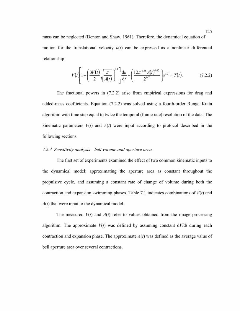
125 mass can be neglected (Denton and Shaw, 1961). Therefore, the dynamical equation of
motion for the translational velocity u(t) can be expressed as a nonlinear differential
relationship:
( ) ( )( )
( ) ( )tTutAtu
tAtVtV =
+
+ 3.1
7.0
65.035.04.1
212
dd
231 ππ . (7.2.2)
The fractional powers in (7.2.2) arise from empirical expressions for drag and
added-mass coefficients. Equation (7.2.2) was solved using a fourth-order Runge–Kutta
algorithm with time step equal to twice the temporal (frame rate) resolution of the data. The
kinematic parameters V(t) and A(t) were input according to protocol described in the
following sections.
7.2.3 Sensitivity analysis—bell volume and aperture area
The first set of experiments examined the effect of two common kinematic inputs to
the dynamical model: approximating the aperture area as constant throughout the
propulsive cycle, and assuming a constant rate of change of volume during both the
contraction and expansion swimming phases. Table 7.1 indicates combinations of V(t) and
A(t) that were input to the dynamical model.
The measured V(t) and A(t) refer to values obtained from the image processing
algorithm. The approximate V(t) was defined by assuming constant dV/dt during each
contraction and expansion phase. The approximate A(t) was defined as the average value of
bell aperture area over several contractions.

126 Data Set Title V(t) A(t)
mVmA (baseline) measured Measured
aVmA approximate Measured
mVaA measured Approximate
aVaA approximate Approximate
Table 7.1 Data set definitions for kinematic inputs in first set of experiments. m, measured; a, approximate; V, volume; A, area; V(t), A(t), see text for
explanation.
7.2.4 Sensitivity analysis—fineness ratio
The second set of experiments examined the effect of using a fineness ratio (bell
height h divided by diameter d) to characterize the bell morphology. The characteristic
diameter d was measured by two methods, using the bell aperture diameter and the
maximum bell diameter. A volume V(t) and area A(t) were assigned to each fineness ratio
measurement using a hemiellipsoid geometrical approximation; the semi-major and minor
axes of the hemiellipsoid correspond to the medusa bell height and radius, respectively.
Based on these kinematic inputs, the results of the dynamical model (equation 7.2.2) were
then compared to the baseline case mVmA defined in table 7.1.
The need to video-record swimming medusae in a non-inertial frame of reference
(i.e., to achieve sufficient image resolution) meant that we were unable to record absolute
position, velocity, and acceleration of the animal. This limitation was circumvented in the
comparative data analyses by referencing these dynamic quantities to the relative maxima
in each experiment.

127
(a)
(b)
Figure 7.2 Measurements of Chrysaora fuscescens swimming. (a) Measured volume versus time. Thick black line, curve fit; thin black line, uncertainty boundaries; gray
line, approximate V(t). (b) Measured aperture area versus time. Thick black line, curve fit; thin black line, uncertainty boundaries; gray line, approximate A(t). Values
are normalized by maximum in the plot.
128 7.3 Results
7.3.1 Bell volume and aperture area approximations
Figure 7.2 plots measured bell volume V and aperture area A with their respective
approximated curves. The amplitude of the volume curve is observed to decrease
throughout the series of propulsive cycles, perhaps as a mechanism for drag reduction at
higher speeds. Although this is of no immediate consequence, it demonstrates the ability of
the measurement technique to capture both transient and long-term effects.
Dynamical model predictions of medusa acceleration, velocity, and position for
each data set defined in table 7.1, are shown in figure 7.3. Data sets mVmA and mVaA show
substantial peaks in acceleration at the beginning of each contraction. This is consistent
with observations by Colin and Costello (2002) for hydromedusae with similar Bauplane.
The remaining two data sets, aVmA and aVaA, do not realize the spikes in acceleration.
They are more qualitatively similar to the acceleration simulated by Daniel (1983). The
velocity and position predictions of the dynamical model, as expected, show a trend similar
to the acceleration. The predicted medusa velocity and position for measured volume cases
mVmA and mVaA show qualitative agreement with previous experimental measurements
(e.g., Costello and Colin, 1994, 1995; Colin and Costello, 2002), whereas the approximated
volume results correspond well with simulated dynamical predictions (e.g., Daniel, 1983).
7.3.2 Fineness ratio approximation
Ultimately, the purpose of the fineness ratio in the dynamical model is to provide an
estimate of bell volume, assuming the bell can be approximated by a hemiellipsoid.
Therefore, it is useful to compare direct fineness ratio measurement with the corresponding
fineness ratio computed from measured volume data.

129 Both data sets are plotted in figure 7.4. The direct measurement appears to
provide a good estimate of the fineness ratio needed to satisfy the ellipsoidal approximation
exactly. The trend of decreasing maximum fineness ratio in each propulsive cycle is similar
to observations of Mitrocoma cellularia and Phialidium gregarium by Colin and Costello
(2002).
(a)
(b)
(c)
Figure 7.3 Dynamical swimming models for each test case. (a) acceleration versus time, (b) velocity versus time, and (c) position versus time. Horizontal bars, mVmA; open diamonds, mVaA; solid black line, aVmA; +, aVaA (see Table 7.1). Values are
normalized by maximum in the plot.

130
Figure 7.4 Measured and computed fineness ratio. Gray line, direct measurement;
black line, values computed from bell volume and aperture measurements using hemiellipsoid approximation.
(a)
(b)
(c)
Figure 7.5 Modeled swimming dynamics from fineness ratio measurement inputs. (a) acceleration, (b) velocity, and (c) position. Gray line, fineness ratio result; black line,
mVmA baseline data set. Values are normalized by maximum in the plot.

131 Using the direct fineness ratio measurement and hemiellipsoid approximation,
bell volume and aperture area were computed. This kinematic data was input to the
dynamical model to compute swimming motions. They are plotted in figure 7.5 and
compared with the baseline data set mVmA.
The swimming dynamics predicted using the fineness-hemiellipsoid approximation
severely overestimate thrust generated by the swimming medusa. Accordingly, the velocity
and position of the animal are also highly overestimated. This result is especially striking
considering that measured fineness ratios appear to agree well with values computed from
the hemiellipsoid approximation.
7.4 Discussion
Two sets of experiments were conducted in this sensitivity analysis to deduce the
effects of kinematic approximations on the accuracy of predicted medusan swimming
dynamics in a momentum flux model of thrust generation. In both cases, bell volume
approximations were observed to agree well with directly measured kinematic inputs to the
dynamical model (e.g., figures 7.2a, 7.4). By contrast, the area approximation was rough,
both qualitatively and quantitatively (figures 7.2b). Interestingly, the crude area
approximation was found to have negligible effect on the accuracy of dynamical model
predictions, whereas the model was observed to be strongly dependent on the volume
approximation. The constant dV/dt approximation in the first set of experiments and the
fineness-hemiellipsoid approximation in the second resulted in severe underestimation and
overestimation, respectively, of thrust generation and associated swimming dynamics from
the model.

132 Although this result might be unexpected from an a priori qualitative study of
the approximations, immediate insight can be gained by examining the quantitative nature
of the model in equations (7.2.1) and (7.2.2). Here we see that thrust is dependent on the
square of the rate of volume change, but only on the first power of area. The fact that the
rate of volume change enters (7.2.1) and not the volume itself suggests that a more
appropriate qualitative check would be comparison of the time derivatives of figures 7.2(a)
and 7.4. There are substantial differences in this parameter between the measured and
approximated volume, especially at the beginning of each contraction and expansion phase.
Errors in the fineness-hemiellipsoid approximation are more complex and depend
on geometrical considerations. It is to be expected that this approximation is most accurate
when the shape of the medusa bell resembles a hemiellipsoid. Fundamental to the fineness-
hemiellipsoid approximation is the assumption that maximum bell diameter occurs at the
bell margin. Under these circumstances, the volume and its rate of change can be
accurately represented. For Chrysaora fuscescens, the bell shape approaches a
hemiellipsoid when in its relaxed state. The maximum bell diameter occurs near the bell
margin, and the fineness ratio can effectively describe the morphology. However, upon
contraction the bell aperture diameter reduces substantially, and the location of maximum
bell diameter is midway between the bell margin and apex. The shape can no longer be
accurately described as a hemiellipsoid. If the bell aperture diameter is still used to define
the fineness ratio, the volume of the medusa is significantly underestimated. The total
volume change during each phase of the propulsive cycle is overestimated, as is the time
rate of volume change. Such was demonstrated in these experiments. Alternatively, one
might attempt to use the maximum bell diameter consistently to define the fineness ratio,

133 but the volume would then be overestimated upon contraction and the time rate of
volume change underestimated.
Using the measured bell volume and aperture area, it is possible to deduce the
proper diameter that should be used to compute the fineness ratio a priori for an accurate
hemiellipsoid approximation. The result is shown in figure 7.6, as the ratio between this
reference diameter and the bell aperture diameter. In addition, the maximum value of bell
diameter on the entire medusa is plotted at points of maximum contraction and expansion.
The variation in reference diameter relative to the bell aperture diameter is subtle,
remaining within 10% of the aperture diameter throughout the series of propulsive cycles.
Nonetheless, using the bell aperture in favor of the reference diameter has been shown to
result in large errors, demonstrating the strong dependence on this parameter.
Consistent with the above arguments, the maximum bell diameter approaches the
bell aperture diameter at points of maximum medusa expansion. By contrast, the maximum
bell diameter is much larger than the reference diameter during phases of maximum
contraction.
Figure 7.6 Ratio of diameter for exact fineness-hemiellipsoid model to bell aperture diameter. Solid black line, diameter ratio; gray circles, maximum bell diameter at
maximum expansion; open circles, maximum bell diameter at maximum contraction.

134 We are left with the dilemma of properly modeling medusan morphology and
swimming in the general case, while maintaining the tractability of the problem. The
measurement algorithm created for this sensitivity analysis presents an alternative, although
it is cumbersome to implement relative to morphological models using geometrical
approximations and a few descriptive parameters. It has been shown here that such models
must have as a priority an accurate representation of medusa bell volume effects, especially
their temporal variation. A single parameter can be insufficient to provide a robust,
accurate description of the animal kinematics. It may be necessary to augment the fineness
ratio description with a parameter to capture the effect of large deformations at the bell
margin. An effective solution may be to incorporate information regarding the location of
maximum bell diameter. This can be accomplished using a truncated-ellipsoid description
of the bell, as a more general case of the hemiellipsoid model. Further examination of the
relationship between volume transients and hydrodynamic forces may suggest more
effective swimming models.
Generally, any dynamic model of locomotion that implements a combination of
kinematic assumptions is vulnerable to a combined effect wherein competing errors of
underestimation and overestimation may go unnoticed in the final result. In the present
study, underestimation of swimming thrust due to the assumption of constant rate of
volume change can be compensated by overestimation of thrust in the fineness-
hemiellipsoid approximation. Should the two errors effectively cancel one another, one
may be led to the spurious conclusion that because the measurements agree with the model,
the theory is sufficient. Therefore it is critical in all animal studies of locomotion to isolate

135 the error associated with each kinematic assumption before implementing them in
combination.
An important step has been taken in this sensitivity analysis to isolate the kinematic
parameters of greatest importance in medusan swimming and to quantify the sensitivity of
the dynamic model to these inputs. More generally, these results urge similar analyses of
other animal locomotion models to avoid potentially misleading results that can arise by
assuming an ipso facto link between kinematic and dynamic similarity.
7.5 Chapter References
Batchelor, G. K. 1967 An Introduction to Fluid Dynamics. Cambridge University Press.
Colin, S. P. and Costello, J. H. 2002 Morphology, swimming performance, and propulsive
mode of six co-occurring hydromedusae. J. Exp. Biol. 205, 427-437.
Costello, J. H. and Colin, S. P. 1994 Morphology, fluid motion and predation by the
scyphomedusa Aurelia aurita. Mar. Biol. 121, 327-334.
Costello, J. H. and Colin, S. P. 1995 Flow and feeding by swimming scyphomedusae. Mar.
Biol. 124, 399-406.
Daniel, T. L. 1983 Mechanics and energetics of medusan jet propulsion. Can. J. Zool. 61,
1406-1420.
Daniel, T. L. 1985 Cost of locomotion: unsteady medusan swimming. J. Exp. Biol. 119,
149-164.
DeMont, M. E. and Gosline, J. M. 1988 Mechanics of jet propulsion in the hydromedusan
jellyfish, Polyorchis penicillatus. I. Mechanical properties of the locomotor
structure. J. Exp. Biol. 134, 313-332.
136 DeMont, M. E. and Gosline, J. M. 1988 Mechanics of jet propulsion in the
hydromedusan jellyfish, Polyorchis penicillatus. II. Energetics of the jet cycle. J.
Exp. Biol. 134, 333-345.
DeMont, M. E. and Gosline, J. M. 1988 Mechanics of jet propulsion in the hydromedusan
jellyfish, Polyorchis penicillatus. III. A natural resonating bell; the presence and
importance of a resonant phenomenon in the locomotor structure. J. Exp. Biol. 134,
347-361.
Denton, E. J. and Shaw, T. I. 1961 The buoyancy of gelatinous marine animals. Proc.
Physiol. Soc. 161, 14-15.
Ford, M. D. and Costello, J. H. 2000 Kinematic comparison of bell contraction by four
species of hydromedusae. Sci. Mar. 64, 47-53.
Ford, M. D., Costello, J. H., Heidelberg, K. B. and Purcell, J. E. 1997 Swimming and
feeding by the schyphomedusa Chrysaora quinquecirrha. Mar. Biol. 129, 355-362.
Gladfelter, W. G. 1972 Structure and function of the locomotory system of the
scyphomedusa Cyanea capillata. Mar. Biol. 14, 150-160.
Hanselman, D. and Littlefield, B. R. 2000 Mastering MATLAB 6. Prentice Hall.
Webb, P. W. 1982 Fast-start resistance of trout. J. Exp. Biol. 96, 93-106.

137
CHAPTER 8: The role of optimal vortex formation in biological fluid
transport
Submitted to Proceedings of the Royal Society of London B October 14, 2004
8.0 Chapter Abstract
Animal phyla that require macro-scale fluid transport for their function have
repeatedly and often independently converged on the use of jet flows. During flow
initiation these jets form fluid vortex rings, which facilitate mass transfer by stationary
pumps (e.g., cardiac chambers) and momentum transfer by mobile systems (e.g., jet-
propelled swimmers). Previous research has shown that vortex rings generated in the
laboratory can be optimized for efficiency or thrust, based on the jet length-to-diameter
ratio (L/D), with peak performance occurring between 3.5 < L/D < 4.5. Attempts to
determine if biological jets achieve this optimization have been inconclusive, due to the
inability to properly account for the diversity of jet kinematics found across animal phyla.
We combine laboratory experiments, in situ observations, and a framework that reduces the
kinematics to a single parameter, in order to show that individual animal kinematics can be
tuned in correlation with optimal vortex ring formation. This new approach facilitates
comparative biological studies of jet flows across animal phyla irrespective of their specific
functions and can be extended to unify theories of optimal jet-based and flapping-based
vortex ring formation.
138 8.1 Introduction
Jet flows in biological systems are typically created by the action of positive
displacement pumps, which eject fluid from a source chamber through a nozzle or orifice
(Vogel, 1994). The flow regime of the jet can be characterized by the velocity of fluid
exiting the chamber (U), the diameter of the jet at the chamber exit (D), and the kinematic
viscosity of the fluid (ν). For Reynolds numbers Re = UD/ν > 6, the period of rapid jet
acceleration during flow initiation causes the leading portion of the jet to roll into a toroidal
fluid mass known as a vortex ring (Cantwell, 1986; see figure 8.1). Laboratory experiments
have demonstrated that the leading vortex makes a proportionally larger contribution to
mass and momentum transport than an equivalent straight jet of fluid (Krueger and Gharib
2003; Dabiri and Gharib 2004). This fact, along with the discovery that physical processes
terminate growth of the leading vortex ring at a jet length-to-diameter ratio between 3.5 <
L/D < 4.5 (Gharib, Rambod and Shariff, 1998; Mohseni and Gharib, 1998), has spurred
interest in the possibility that biological systems may optimize vortex formation for
effective fluid transport (Gharib et al., 1998; Mohseni, Ran and Colonius, 2001; Linden and
Turner, 2001; Krueger and Gharib, 2003; Linden and Turner, 2004; Dabiri and Gharib,
2004).
Inferences drawn from vortex rings generated in the laboratory are limited due to
kinematic constraints on the vortex generators. Typically the vortices are created by
ejecting fluid through a tube with constant exit diameter (Didden, 1979; Gharib et al., 1998;
Krueger and Gharib, 2003; Dabiri and Gharib, 2004). This is in contrast with the complex,
time-dependent kinematics of positive displacement pumps found in nature (e.g., Vogel,
1994). In situ measurements of fluid jet length-to-diameter ratio (L/D, hereafter referred to

139 as the dimensionless “formation time” following Gharib et al., 1998) have suffered
from an inability to unambiguously incorporate the observed time-varying exit diameter
D(t). Attempts to reduce the observed kinematics using a time-averaged exit diameter ( D )
have been unsuccessful in determining a clear correlation between vortex formation
dynamics and animal kinematics (e.g., Bartol, Patterson and Mann 2001; Linden and
Turner 2004).
The average jet diameter is by itself an insufficient index of jet kinematics because
it lacks critical information regarding temporal trends in the jet exit diameter. As mentioned
above, laboratory experiments have pointed to the existence of a critical formation time
after which growth of the leading vortex ring ceases, and any additional fluid ejected takes
the form of a trailing straight jet (Gharib et al., 1998). Since this vortex-limiting formation
time is dictated by the time-history of the jet exit diameter and not its average value, an
effective kinematic index must preserve this information. From this we can properly record
how jet flow is manipulated by changes in the exit diameter both before and after the
vortex-limiting formation time is reached.
The goal of this paper is to combine laboratory experiments, in situ observations,
and a framework that reduces the kinematics to a single parameter, in order to show that
individual animal kinematics can be tuned in correlation with optimal vortex ring
formation.

140 8.2 Methods
8.2.1 Kinematic analysis
A suitable kinematic parameter to describe observed animal motions can be derived
by considering an infinitesimal increment in the formation time, ∆(L/D)* ≡ (U(τ)/D(τ))∆τ,
where ∆τ is a small increment in dimensional time. Here the jet exit velocity and diameter
are instantaneous values at time τ. Integrating the formation time increment from flow
initiation at τ = 0 to termination at τ = t, we arrive at a parameter for vortex formation that
effectively incorporates time-dependent jet kinematics: (L/D)* ≡ DU t. The over-bar again
denotes a time average, and t is the duration of fluid ejection.
For the case of a constant jet exit diameter, this new index is identical to the
traditional definition. In addition, when the exit velocity and diameter follow the same
temporal trend (e.g., both linearly increasing) the new index also gives the same result as
the traditional definition. This occurs because the parameter is dimensionless and therefore
does not account for overall changes in the scale of the fluid transport mechanism. The
benefit of this property of the parameter is that it facilitates comparison between biological
systems of differing function, morphology, and scale. Conversely, the parameter is limited
in that it does not account for changes in the fluid dynamics due to Reynolds number
effects. However Gharib et al. (1998) demonstrated that the process of vortex ring
formation is relatively insensitive to the Reynolds number of the flow.
Although the new index also involves a time average, the velocity and diameter
data are properly coupled in the calculation. In contrast, previous time-averaging
techniques treated the exit velocity and diameter data as independent trends. It is that

141 decoupling that has led to spurious conclusions regarding the correlation between
vortex formation and animal pump kinematics.
8.2.2 Laboratory apparatus
To test this result experimentally, we studied jet flow vortex formation by creating
an apparatus that incorporates a controllable variable-diameter exit nozzle on the flow tube
of a traditional laboratory vortex generator (figure 8.1, cf. Dabiri and Gharib, 2005). This
technique was used to probe the effects of a temporally increasing exit diameter on jet
flows as is observed, for example, during tail-first swimming motions of squid (O’Dor,
1988; Anderson and DeMont, 2000; Bartol et al., 2001) and the early refilling phase of
ventricular diastole (Verdonck, et al., 1996). Fluid forces were determined from the time-
integrated jet thrust, or fluid impulse, . This first moment of vorticity
was computed given the position vector (x) of fluid particles relative to the nozzle exit
plane and axis of symmetry, the velocity field (u) measured using digital particle image
velocimetry (Willert and Gharib, 1991), and the measurement volume (V).
( )∫ ×∇×=V
VI dux
8.3 Results
8.3.1 Laboratory results
Importantly, measurements showed that temporal increases in jet exit diameter do
not change the vortex-limiting formation time (now computed using (L/D)*) from the
constant-diameter value of 4.0 ± 0.5 (cf. Dabiri and Gharib, 2005). This observed
robustness of the vortex formation process for the various jet kinematics tested suggests
that conclusions regarding the fluid dynamics can be applied beyond the specific
kinematics of this experimental apparatus.

142 Temporal increases in jet exit diameter during formation of the leading vortex
ring were found to increase thrust and impulse generated by the apparatus by increasing the
moment arm of the generated vorticity flux. This effect is predicted by a thin vortex ring
model of the flow (Shariff and Leonard, 1992), in which the impulse can be approximated
from the vortex ring circulation (area-integrated vorticity, Γ) and diameter (DR), as
I = ¼πΓDR2. Figure 8.2 indicates that the radial extent DR of the leading vortex rings
increased in proportion to temporal growth of the jet exit diameter.
Figure 8.1 Schematic of jet flow apparatus with time-varying nozzle exit diameter. All components are depicted as they appear in a meridian cross-section of the
axisymmetric device. Nozzle actuators are not shown. Jet flow at the exit plane (i.e., through the origin and normal to the symmetry axis) is from left to right. Jet was
initiated upstream using a piston-cylinder mechanism (cf. Gharib et al., 1998) that impulsively created a constant volume flux of 8.8 cm3s-1, with a rise time of 300 ms.
Nozzle exit diameter was varied temporally between 45% and 67% of the inlet diameter, Dinlet = 2.54 cm, in each experiment. Variables indicated in the schematic
are referred to in the text.
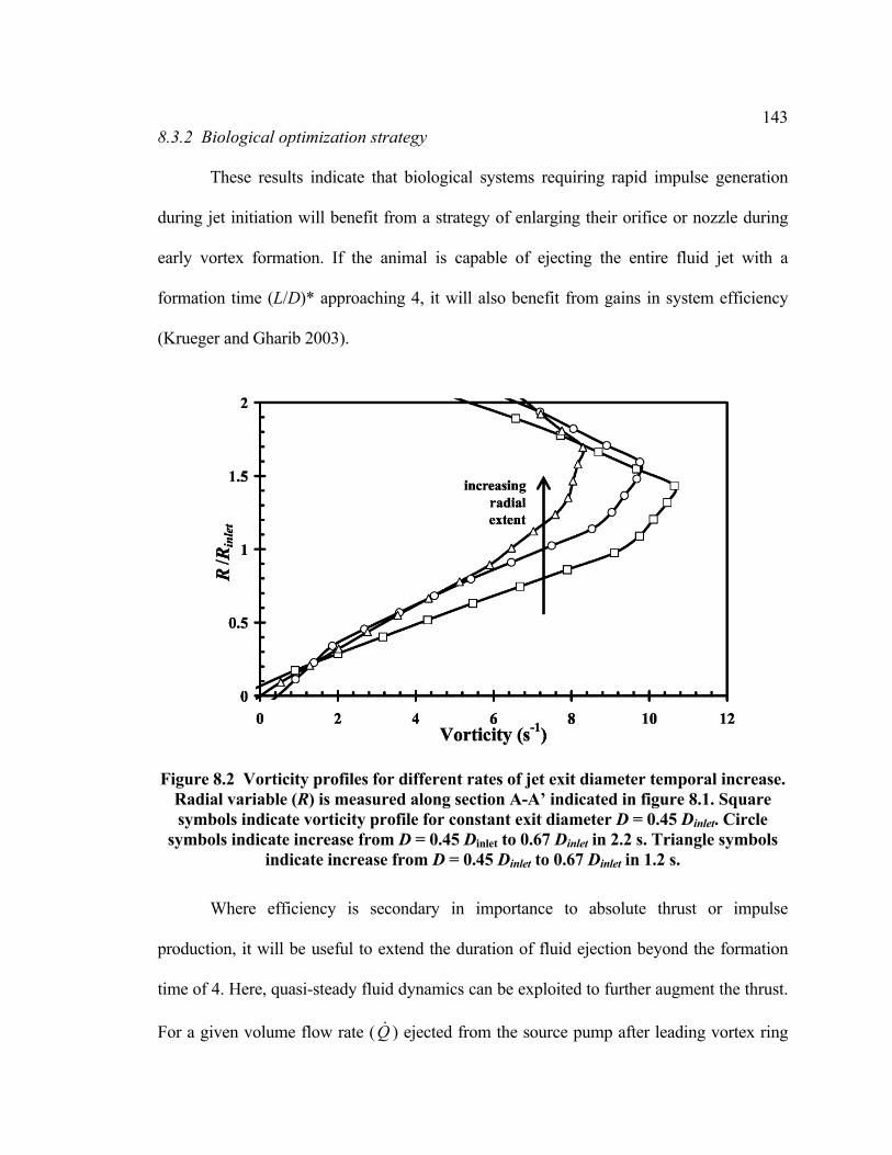
143 8.3.2 Biological optimization strategy
These results indicate that biological systems requiring rapid impulse generation
during jet initiation will benefit from a strategy of enlarging their orifice or nozzle during
early vortex formation. If the animal is capable of ejecting the entire fluid jet with a
formation time (L/D)* approaching 4, it will also benefit from gains in system efficiency
(Krueger and Gharib 2003).
Figure 8.2 Vorticity profiles for different rates of jet exit diameter temporal increase. Radial variable (R) is measured along section A-A’ indicated in figure 8.1. Square symbols indicate vorticity profile for constant exit diameter D = 0.45 Dinlet. Circle
symbols indicate increase from D = 0.45 Dinlet to 0.67 Dinlet in 2.2 s. Triangle symbols indicate increase from D = 0.45 Dinlet to 0.67 Dinlet in 1.2 s.
Where efficiency is secondary in importance to absolute thrust or impulse
production, it will be useful to extend the duration of fluid ejection beyond the formation
time of 4. Here, quasi-steady fluid dynamics can be exploited to further augment the thrust.
For a given volume flow rate ( ) ejected from the source pump after leading vortex ring Q&

144 growth has terminated, the exit flow velocity will be inversely proportional to the
square of the exit diameter, U ~ /DQ& 2. Since the rate of fluid impulse production is
proportional to U2, decreasing the exit diameter after growth of the leading vortex ring has
ceased will provide substantial gains in momentum transport by the jet flow.
In sum, animals that face selective pressures for efficiency will create flows with jet
formation times approaching 4. Conversely, systems that require large thrust production—
possibly at the expense of operational efficiency—will increase the exit diameter until a
formation time of 4 is achieved, and then subsequently decrease the exit diameter for
optimal performance during extended fluid ejection.
8.3.3 Comparison with in situ squid measurements
We confirmed these predictions for two biological systems on opposite ends of the
spectrum (functionally speaking) of biological jet flows. In the first case, we considered
tail-first swimming of the brief squid Lolliguncula brevis. This mode of locomotion is
employed by squid for high-speed maneuvers, including their jet-propelled escape
mechanism (Gosline and DeMont, 1985; O’Dor, 1988; Anderson and DeMont, 2000;
Bartol et al., 2001). A premium is accordingly placed on thrust production during this
swimming mode. Following the foregoing discussion, the formation time should be larger
than 4, with a transition from temporally increasing squid funnel exit diameter to temporal
decrease occurring near the vortex-limiting formation time. Figure 8.3 plots data from
published measurements of the time dependent funnel exit diameter during successive
swimming cycles (i.e., Bartol et al. 2001) versus jet formation times computed using the
methods presented above. When the funnel exit diameter is plotted versus the traditional
formation time definition (L/ D ), there is no clear correlation between changes in the

145 funnel exit diameter and the vortex-limiting formation time (crosses). However, using
the parameter (L/D)* developed here, a sharper transition between initial funnel exit
diameter increase and subsequent decrease is observed (closed circles). Furthermore, the
transition between the two phases follows the predicted behavior, occurring in the range 3.5
< (L/D)* < 4.5.
Figure 8.3 Tail-first swimming kinematics of Lolliguncula brevis. Jet exit diameter and velocity data from successive swimming cycles were compiled from Bartol et al.
2001. Dashed vertical lines indicate range of vortex-limiting formation time, 3.5 < (L/D)* < 4.5. Cross symbols indicate trends computed using L/ D defined in the text.
Circle symbols and solid line indicate trend computed using (L/D)* defined in the text.
8.3.4 Comparison with in vivo cardiac measurements
As a second example, we examined published data from trans-mitral blood flow
during early left ventricle diastolic filling in patients (i.e., Verdonck et al., 1996) measured
using M-mode echocardiography (Nishimura et al., 1989). Figure 8.4 plots the mitral valve

146 exit diameter versus jet formation time (L/D)* computed for normal and pathological
conditions observed in the patients.
During normal function (solid line), the entire jet is ejected in a formation time less
than 4, indicating efficient operation. The initial rate of valve opening increases with heart
rate (closed circles), providing the augmented fluid impulse required under the systemic
stress. When those stresses are exacerbated, as in pathologies such as cardiac ischemia
(Gaasch and Zile 2004), a response is observed in the mitral valve kinematics in which the
degree of temporal valve opening is increased (closed squares). Again this is in accord with
the principles we have outlined whereby such temporal increases in jet diameter provide
increased impulse generation. Although this compensatory mechanism can be effective in
the short term, further deterioration of the pump mechanism in the form of reduced
performance at flow initiation (i.e., reduced E/A wave ratio; Appleton, Hatle and Popp,
1988) can force the system to abandon efficient function for the sake of merely producing
sufficient fluid impulse to survive. In these cases, the jet formation time is increased
beyond (L/D)* ≈ 4 (closed triangles). Similar to the behavior observed in the squid jet
flows, the resulting exit diameter kinematics follow our prediction of a temporally
increasing exit diameter until the vortex-limiting formation time is reached, followed by
temporal decrease thereafter.
Certainly, not all pathologies of left ventricle diastole can exploit these
compensatory mechanisms. When the function of the valves themselves is affected as in
mitral valve stenosis (Gaasch and Zile 2004), any correlation between valve kinematics and
the vortex-limiting formation time is lost (dashed line). However, this observation in itself
serves as a useful diagnostic for pathologies that are localized near the jet exit plane.

147
Figure 8.4 Trans-mitral flow during normal and pathological early diastolic filling. Jet exit diameter and velocity data for each patient were compiled from Verdonck et
al., 1996. Diameter data are normalized by the time-averaged mitral valve exit diameter in each patient to facilitate quantitative comparison. Dashed vertical line indicates lower bound of vortex-limiting formation time, (L/D)* = 3.5. Open circle
symbols indicate points of correlation with optimal vortex formation time.
8.4 Discussion
This work has shown that functionally and morphologically diverse biological fluid
transport systems can be designed and tuned in accordance with the dynamics of vortex
ring formation. The framework introduced here for studying biological jet flows has the
potential to connect functionally disparate systems in comparative studies and to improve
our understanding of jet flow pathologies relative to normal function.
We also suggest that the analytical method developed here can be used to develop a
connection between the observed robustness of jet-based vortex ring formation in aquatic

148 propulsion (Linden and Turner 2004) and the previously discovered optimal Strouhal
parameter for flapping-based vortex ring formation in insect and bird flight (Taylor, Nudds
and Thomas 2003). In an analysis of the latter group, the jet exit diameter of relevance in
the present paper will be replaced with considerations for the time-dependent flap
morphology and flapping kinematics.
8.5 Chapter References
Anderson, E. J. and DeMont, M. E. 2000 The mechanics of locomotion in the squid Loligo
pealei: locomotory function and unsteady hydrodynamics of the jet and intramantle
pressure. J. Exp. Biol. 203, 2851-2863.
Appleton, C. R., Hatle, L. K. and Popp, R. L. 1988 Relation of transmitral flow velocity
patterns to left ventricular diastolic function: new insights from a combined
hemodynamic and Doppler echocardiographic study. J. Am. Col. Cardiol. 12, 426-
440.
Bartol, I. K., Patterson, M. R. and Mann, R. 2001 Swimming mechanics and behaviour of
the shallow-water brief squid Lolliguncula brevis. J. Exp. Biol. 204, 3655-3682.
Cantwell, B. J. 1986 Viscous starting jets. J. Fluid Mech. 173, 159-189.
Dabiri, J. O. and Gharib, M. 2004 Fluid entrainment by isolated vortex rings. J. Fluid
Mech. 511, 311-331.
Dabiri, J. O. and Gharib, M. 2005 Starting flow through nozzles with temporally variable
exit diameter. J. Fluid Mech., in press.
Didden, N. 1979 Formation of vortex rings—rolling-up and production of circulation. Z.
Angew. Math. Phys. 30, 101-116.

149 Gaasch, W. H. and Zile, M. R. 2004 Left ventricular diastolic dysfunction and diastolic
heart failure. Annu. Rev. Med. 55, 373-394.
Gharib, M., Rambod, E. and Shariff, K. 1998 A universal time scale for vortex ring
formation. J. Fluid Mech. 360, 121-140.
Gosline, J. M. and DeMont, M. E. 1985 Jet-propelled swimming in squids. Scient. Am. 252,
96-103.
Krueger, P. S. and Gharib, M. 2003 The significance of vortex ring formation to the thrust
and impulse of a starting jet. Phys. Fluids 15, 1271-1281.
Linden, P. F. and Turner, J. S. 2001 The formation of ‘optimal’ vortex rings, and the
efficiency of propulsion devices. J. Fluid Mech. 427, 61-72.
Linden, P. F. and Turner, J. S. 2004 ‘Optimal’ vortex rings and aquatic propulsion
mechanisms. P. Roy. Soc. Lond. B 271, 647-653.
Mohseni, K. and Gharib, M. 1998 A model for universal time scale of vortex ring
formation. Phys. Fluids 10, 2436-2438.
Mohseni, K., Ran, H. Y. and Colonius, T. 2001 Numerical experiments on vortex ring
formation. J. Fluid Mech. 430, 267-282.
Nishimura, R. A., Abel, M. D., Hatle, L. K. and Tajik, A. J. 1989 Assessment of diastolic
function of the heart: background and current applications of Doppler
echocardiography. Part 2: clinical studies. Mayo Clin. Proc. 64, 181-204.
O’Dor, R. K. 1988 The forces acting on swimming squid. J. Exp. Biol. 137, 421-442.
Shariff, K. and Leonard, A. 1992 Vortex rings. Annu. Rev. Fluid Mech. 24, 235-279.
Taylor, G. K., Nudds, R. L. and Thomas, A. L. R. 2003 Flying and swimming animals
cruise at a Strouhal number tuned for high power efficiency. Nature 425, 707-711.

150 Verdonck, P., Segers, P., Missault, L. and Verhoeven, R. 1996 In vivo validation of a
fluid dynamics model of mitral valve M-mode echocardiogram. Med. Biol. Eng.
Comput. 34, 192-198.
Vogel, S. 1994 Life in Moving Fluids. Princeton University Press.
Willert, C. E. and Gharib, M. 1991 Digital particle image velocimetry. Exp. Fluids 10, 181-
193.

151
CHAPTER 9: Flow patterns generated by oblate medusan jellyfish: field
measurements and laboratory analyses
Submitted to Journal of Experimental Biology November 12, 2004
9.0 Chapter Abstract
Flow patterns generated by medusan swimmers such as jellyfish are known to differ
according to the morphology of the various animal species. Oblate medusae have been
previously observed to generate vortex ring structures during the propulsive cycle. Due to
the inherent physical coupling between locomotor and feeding structures in these animals,
the dynamics of vortex ring formation must be robustly tuned to facilitate effective function
of both systems. To understand how this is achieved, we employed dye visualization
techniques on swimming scyphomedusae (Aurelia aurita) observed swimming in their
natural marine habitat. The flow created during each propulsive cycle consists of a toroidal
starting vortex formed during the power swimming stroke, followed by a stopping vortex
of opposite rotational sense generated during the recovery stroke. These two vortices merge
in a laterally-oriented vortex superstructure that induces flow both toward the subumbrellar
feeding surfaces and downstream. The lateral vortex motif discovered here appears to be
critical to the dual function of the medusa bell as a flow source for feeding and propulsion.
Furthermore, vortices in the animal wake exhibit greater volume and closer spacing than
predicted by prevailing models of medusan swimming. These effects are shown to be
advantageous for feeding and swimming performance and are an important consequence of
vortex interactions that have been previously neglected.

152
9.1 Introduction
Medusan swimmers propel themselves forward via periodic bell contractions that
act to decrease the volume of their subumbrellar cavity and jet water out of the oral end of
their bell. Described as jet propulsion, prevailing models of this process focus on the fluid
efflux that emerges during bell contraction: a toroidal volume of rotating fluid known as the
power stroke starting vortex ring (figure 9.1).
Any vortex formation that may occur during the recovery stroke of the propulsive
cycle is neglected in existing models of the swimming process (e.g., Daniel, 1983; Colin
and Costello, 2002; McHenry and Jed, 2003). Therefore interactions between adjacent
vortex rings in the wake have been previously examined based on the assumption of a
uniform train of starting vortex rings in the animal wake, each with identical rotational
sense.
Weihs (1977) uses a quasi-steady model of such a vortex ring train to conclude that
substantial thrust augmentation can occur—up to 150% relative to a steady jet—if the
vortex rings are spaced sufficiently close together (i.e., C/(B+D) is small; see figure 9.1).
The thrust benefit arises due to the induced downstream velocity of the vortex ring train on
each of its members. Interestingly, the flow pattern depicted by Ford et al. (figure 5, 1997)
for the oblate jellyfish Chrysaora quinquecirrha shows a train of closely spaced vortex
rings.
The proximity of the wake vortex rings to each other and to the swimming animal
as measured by Ford et al. (1997) is unexpected given the tendency of individual vortex
rings to rapidly propagate away from the flow source due to self-induced velocity (Lamb,
1932) and convection by any jet-like flow that is present behind each ring. An estimate by
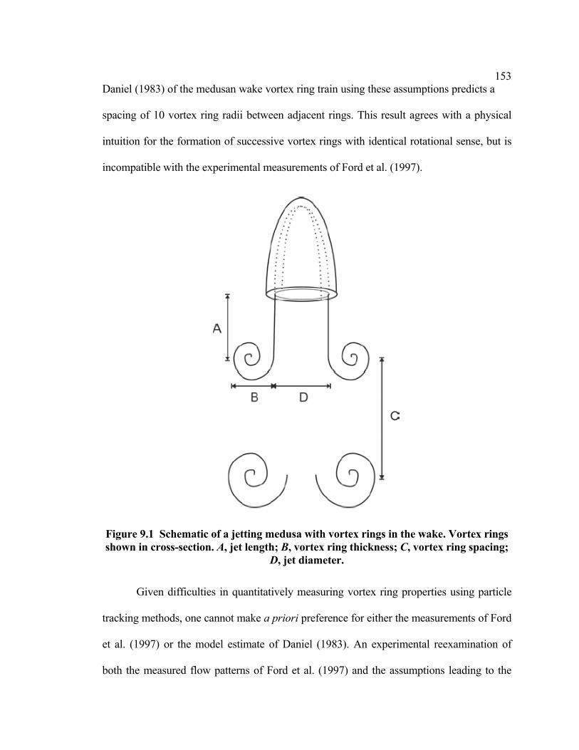
153 Daniel (1983) of the medusan wake vortex ring train using these assumptions predicts a
spacing of 10 vortex ring radii between adjacent rings. This result agrees with a physical
intuition for the formation of successive vortex rings with identical rotational sense, but is
incompatible with the experimental measurements of Ford et al. (1997).
Figure 9.1 Schematic of a jetting medusa with vortex rings in the wake. Vortex rings shown in cross-section. A, jet length; B, vortex ring thickness; C, vortex ring spacing;
D, jet diameter.
Given difficulties in quantitatively measuring vortex ring properties using particle
tracking methods, one cannot make a priori preference for either the measurements of Ford
et al. (1997) or the model estimate of Daniel (1983). An experimental reexamination of
both the measured flow patterns of Ford et al. (1997) and the assumptions leading to the
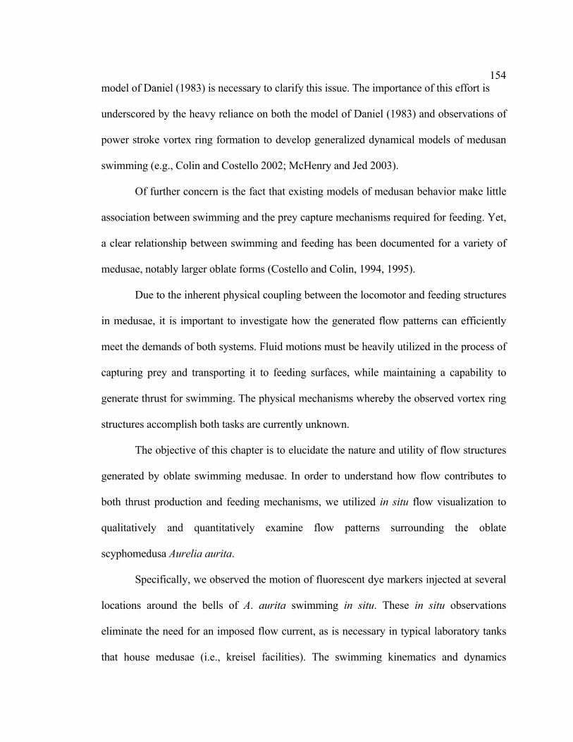
154 model of Daniel (1983) is necessary to clarify this issue. The importance of this effort is
underscored by the heavy reliance on both the model of Daniel (1983) and observations of
power stroke vortex ring formation to develop generalized dynamical models of medusan
swimming (e.g., Colin and Costello 2002; McHenry and Jed 2003).
Of further concern is the fact that existing models of medusan behavior make little
association between swimming and the prey capture mechanisms required for feeding. Yet,
a clear relationship between swimming and feeding has been documented for a variety of
medusae, notably larger oblate forms (Costello and Colin, 1994, 1995).
Due to the inherent physical coupling between the locomotor and feeding structures
in medusae, it is important to investigate how the generated flow patterns can efficiently
meet the demands of both systems. Fluid motions must be heavily utilized in the process of
capturing prey and transporting it to feeding surfaces, while maintaining a capability to
generate thrust for swimming. The physical mechanisms whereby the observed vortex ring
structures accomplish both tasks are currently unknown.
The objective of this chapter is to elucidate the nature and utility of flow structures
generated by oblate swimming medusae. In order to understand how flow contributes to
both thrust production and feeding mechanisms, we utilized in situ flow visualization to
qualitatively and quantitatively examine flow patterns surrounding the oblate
scyphomedusa Aurelia aurita.
Specifically, we observed the motion of fluorescent dye markers injected at several
locations around the bells of A. aurita swimming in situ. These in situ observations
eliminate the need for an imposed flow current, as is necessary in typical laboratory tanks
that house medusae (i.e., kreisel facilities). The swimming kinematics and dynamics

155 measured by this method should be more relevant to animal behavior in the marine
water column than compared to those achieved by any type of laboratory tank. Further, the
use of a continuous dye marker instead of discrete prey for particle tracking simplifies the
identification of large-scale fluid structures in the flow, such as vortex rings. In addition,
the three dimensional nature of the flow (in the absence of significant vortex stretching)
does not limit the effectiveness of the dye marker technique, as is the case with particle
tracking. By observing vortex dynamics in the wake and fluid-structure interactions near
the medusa bell, the role of the observed flow structures is clarified.
9.2 Methods
9.2.1 Video measurements
Field data were collected from a marine lake (145 hectares, maximum depth 46 m)
on the island of Mljet, Croatia, located in the Adriatic Sea (Lat: 42.75º N Long: 17.55º E)
during July 2003. All of the video was taken in shallow water (< 20 m) by SCUBA using
natural light. Video recordings followed the methods of Costello et al. (1998), whereby
medusae were videotaped on miniDV videotape using a Sony DCR VX2000 camera with a
zoom lens contained within an Amphibico underwater housing. A second diver injected 20
µl pulses of concentrated fluorescene dye into the fluid at specific locations around the
medusae. This second diver was located to the side of the medusae at 90° to the orientation
of the video camera. Both divers took care to avoid disturbing the fluid around the medusa
being video taped. The dye made any disturbances by the divers obvious allowing these
shots to be excluded from the video analysis. The length of the pipette used to administer
the dye (approximately 4 cm) was used as a calibrating size scale in later analysis.

156 Several hours of video were recorded in which medusae were observed
swimming both in large groups and in isolation. The swimming kinematics were
qualitatively consistent throughout the observations using the dye technique. In order to
achieve more quantitative results, a subset of the full video database was analyzed in
greater detail.
9.2.2 Kinematic analyses
Select recordings of animal swimming in the field were collected for further
laboratory analysis. For kinematic analyses, sequences of recorded swimming motions in
two medusae were chosen according to visibility of the medusa subumbrellar surface,
motion in planes parallel to the camera, separation from other medusae, and sufficient dye
marker in the flow. In addition, the upper and lower limits of animal size were sought to
facilitate comparisons of fluid dynamic and geometric scaling. The larger medusa in the
kinematic analyses is an order of magnitude larger than the smaller medusa (10.2-cm
maximum bell diameter versus 3.6-cm maximum bell diameter, or 22 times larger by
volume).
Video recordings of up to 5 successive swimming contractions in each animal were
analyzed using the algorithm of Dabiri and Gharib (2003). Between 10 and 20 control
points along the subumbrellar surface of each medusa were tracked during swimming
motions to generate a computational reconstruction of the medusae kinematics. The entire
subumbrellar surface was clearly visible through the transparent mesoglea in each of the
selected frames, and any fluorescent dye carried inside the medusa bell further improved
the resolution of the interface location.

157 In addition to measuring the shape of the bell, the properties of the formed
vortex rings were analyzed. Specifically, the volume of each vortex ring and the inter-ring
spacing of the vortex ring train in the animal wake were measured. The physical extent of
each vortex ring was measured based on the distribution of the dye marker in the flow.
The kinematic analyses include only frames in which the animals are swimming
parallel to the image plane of the camera. Hence, the orientation of the vortex rings can be
assumed to be such that the ring axis is also parallel to the image plane. To calculate the
volume of the visible toroidal vortex rings, we therefore require only measurements of the
diameter across the toroid (B+D in figure 9.1) and the diameter of the vortex core (B in
figure 9.1).
Important caveats associated with this measurement technique are discussed in the
following section. Each set of measurements is presented conservatively, with an
uncertainty calculated as the maximum difference between any individual measurement
and the average of the set. This metric is used in lieu of the standard deviation, since the
standard deviation tends to underestimate the data spread for relatively small sample sizes
such as those studied here (Freeman et al., 1998).
9.2.3 Strategies for dye marker interpretation
Despite the convenience of a passive dye marker for qualitative flow visualization,
there are important limitations to the technique. First, although all of the dye labels fluid,
not all of the fluid is labeled by dye. Therefore if one desires to track the evolution of a
fluid structure such as a vortex ring using the passive dye marker, the visible labeled
structure may be smaller than the actual fluid structure. When identifying vortex rings in
the flow, the dye-labeled ring represents a lower bound on the size of the vortex.
158 Secondly, the diffusion coefficient of dye markers such as that used in these
experiments (fluorescene) is substantially less than the diffusion coefficient of fluid
vorticity (i.e., rotation and shear), as measured by the kinematic viscosity of water (~ 10-2
cm2s-1). Hence, regions of compact vorticity such as the wake vortex rings will tend to
spread by diffusion at a rate faster than can be observed in the dye. Again, the result is that
the visibly labeled structure may be smaller than the actual fluid structure. Consequently,
all of our estimates of vortex ring volume are conservative values.
Our strategy is to exploit these limitations by assuming that the measurements
represent a lower bound on the size of the vortex rings. The effects of a departure from the
lower bound case can be inferred from the available data.
9.3 Results
9.3.1 Vortex formation process
The swimming cycle of Aurelia aurita consists of a bell contraction phase (i.e.,
power stroke) and a bell relaxation phase (i.e., recovery stroke). Observations of
fluorescent dye that was injected into the fluid outside the bell along the bell margin of
swimming A. aurita revealed that the two phases of the swimming cycle interacted with the
surrounding fluid to form distinct vortex rings at separate locations relative to the bell.
During the power stroke the bell contracted and initiated the formation of a starting
vortex ring. The starting vortex ring induced a motion of fluid originating from regions
both inside the subumbrellar volume and outside the bell via entrainment of ambient fluid.
The direction of induced motion was oriented at an angle away from the bell margin and
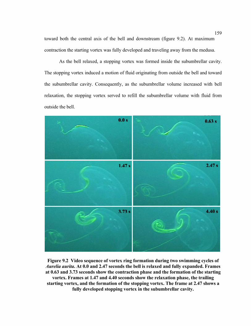
159 toward both the central axis of the bell and downstream (figure 9.2). At maximum
contraction the starting vortex was fully developed and traveling away from the medusa.
As the bell relaxed, a stopping vortex was formed inside the subumbrellar cavity.
The stopping vortex induced a motion of fluid originating from outside the bell and toward
the subumbrellar cavity. Consequently, as the subumbrellar volume increased with bell
relaxation, the stopping vortex served to refill the subumbrellar volume with fluid from
outside the bell.
Figure 9.2 Video sequence of vortex ring formation during two swimming cycles of Aurelia aurita. At 0.0 and 2.47 seconds the bell is relaxed and fully expanded. Frames at 0.63 and 3.73 seconds show the contraction phase and the formation of the starting
vortex. Frames at 1.47 and 4.40 seconds show the relaxation phase, the trailing starting vortex, and the formation of the stopping vortex. The frame at 2.47 shows a
fully developed stopping vortex in the subumbrellar cavity.
160
The stopping vortex remained in the subumbrellar cavity during the beginning of
the contraction phase of the next swimming cycle. As the bell contracted, a part of the
stopping vortex ring was ejected out from the subumbrellar cavity and interacted with the
starting vortex of the new cycle. In the interaction, a portion of the fluid from the stopping
vortex co-joined with the starting vortex ring, completing formation of the downstream
lateral vortex superstructure. The kinematics of the starting, stopping, and co-joined lateral
vortex structure are illustrated in figure 9.3.
Although the schematic in figure 9.3(b) suggests a clear distinction between power
and recovery stroke vortices in the wake, the two components actually become highly
amalgamated due to fluid mixing. This process makes the individual vortices increasingly
difficult to distinguish as the wake develops.

161
(b) (a)
(c)
Figure 9.3 Kinematics of the starting, stopping, and co-joined lateral vortex structures. (a) Image of medusa vortex wake. (b) Corresponding schematic of medusa vortex wake. P, power stroke starting vortex ring; R, recovery stroke stopping vortex ring; L1/L2, adjacent lateral vortex superstructures. (c) Flow paths in vortex wake.
Solid arrows indicate directions of vortex rotation. Dashed arrows indicate flow induced by vortex rotation.
There are several important observations to be made from the qualitative analysis of
the formation and interaction of the starting and stopping vortex rings during swimming
cycles. First, throughout the swim cycle, from the onset of the contraction phase through
the relaxation phase, there is a continual flow of water from outside the bell, adjacent to the
bell margin. During the contraction, the flow contributes to the fluid in the starting vortex
ring, but during bell relaxation it contributes to the fluid in the stopping vortex ring.

162 Second, during a sequence of propulsive cycles we observed that the stopping vortex
ring from the preceding lateral vortex structure persists in the bell and contributes to the
formation of the subsequent starting vortex (figure 9.2). A complex interaction occurs as
the starting vortex ring grows and the previous stopping vortex is convected downstream
away from the bell margin. The interaction appears to increase the volume but decrease the
velocity of the starting vortex ring, via cancellation of starting vortex vorticity by the
preceding stopping vortex ring of opposite rotational sense (cf. Lim and Nickels, 1995). As
a result of this interaction, the vortex ring volume and vortex ring spacing of swimming
oblate medusae do not relate to thrust in the manner predicted for a unidirectional pulsed jet
of fluid through an orifice (i.e., Table 9.1). Existing models for the time-dependent thrust
neglect recovery stroke vortex formation altogether and therefore do not apply to these
medusae.
The interaction between starting and stopping vortices described above tends to
increase the total momentum of each wake vortex. This is because the mass of each wake
vortex increases (i.e., the starting and stopping vortex masses combine in the wake) to a
greater degree than the wake vortex velocity decreases via vorticity cancellation. The effect
of vorticity cancellation is limited because it is a viscosity-dependent process that occurs
only at the interface between the starting and stopping vortices (Shariff and Leonard,
1992).
Dye injected into the middle of the subumbrellar volume is not ejected directly
outwards during bell contraction but instead spreads laterally along the subumbrellar
surface of the bell. All of the dye leaves the subumbrellar cavity at the bell margin.
However, it takes the medusa several swim cycles to eject all of the dye from the

163 subumbrellar region. No fluid is ever directly ejected from the central subumbrellar
region. In fact, there is always a net flow into the subumbrellar cavity in the central portion
trailing to the bell. This is due to the direction of rotation of the stopping vortex ring in this
region (figure 9.3).
9.3.2 Tentacle positioning
Throughout the pulsation cycle the tentacles of A. aurita were primarily located in
vortex rings (figure 9.4). At the beginning of the contraction phase they were in the
subumbrellar cavity in the stopping vortex ring. As the bell contracted the tentacles became
entrained in the starting vortex ring, which oriented the tentacles in a trailing position. At
the end of the contraction phase and the onset of the relaxation phase, the tentacles became
entrained in the stopping vortex ring, which drew them back up into the subumbrellar
cavity.
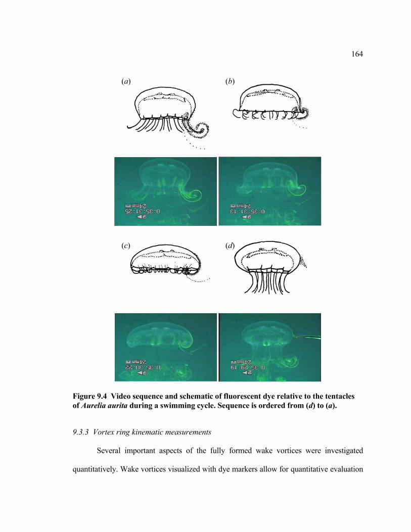
164
(a) (b)
(c) (d)
Figure 9.4 Video sequence and schematic of fluorescent dye relative to the tentacles of Aurelia aurita during a swimming cycle. Sequence is ordered from (d) to (a).
9.3.3 Vortex ring kinematic measurements
Several important aspects of the fully formed wake vortices were investigated
quantitatively. Wake vortices visualized with dye markers allow for quantitative evaluation
165 of thrust production mechanisms. In this regard, an important variable is the volume of
each wake vortex ring relative to the volume of fluid ejected by the medusa. Although the
results of the preceding section suggest a more complex relationship between swimming
thrust and vortex kinematics than has been previously appreciated, we can anticipate that,
for a fixed swimming frequency (and corresponding characteristic flow velocity),
swimming thrust will maintain a direct relationship with vortex volume (cf. Daniel, 1983).
We cannot neglect the fact that the characteristic flow velocity is reduced by vorticity
cancellation between the starting and stopping vortices. However, as mentioned previously,
this effect is limited in the present case. Therefore, volume measurements provide the most
useful index of swimming thrust in the present study.
The volume contained by the bell at full contraction and relaxation was measured
using the subumbrellar surface profiles obtained from the video analysis. The difference
between these two values gives the volume of fluid ejected. The ratio of wake vortex ring
volume, Ωw, to ejected fluid volume, Ωb, was relatively insensitive to animal size: 3.09 ±
0.35 for the smaller animal, and 3.57 ± 0.40 for the larger. Two primary effects contribute
to the large volume of the wake vortex rings relative to the volume of fluid ejected. First of
these is the presence of the stopping vortex ring, which is created from fluid external to the
bell. This stopping vortex is complexed with the starting vortex ring of the subsequent
lateral vortex to create each wake vortex ring. Secondly, both starting and stopping vortex
ring formation processes involve substantial entrainment of ambient fluid from outside the
bell.
Given the vortex ring kinematic measurements, we can also determine the interring
spacing in the wake vortex ring train. In both the larger and smaller medusa, the wake

166 vortex rings are very closely spaced. The inter-ring spacing is 1.36 ± 0.08 ring radii in
the smaller medusa and 1.06 ± 0.06 ring radii in the large medusa.
9.4 Discussion
9.4.1 Implications for medusan swimming behavior
Dye studies of the swimming oblate medusa, Aurelia aurita, demonstrated the
formation of two vortex rings during each bell pulsation cycle. As expected, we observed
the formation of a starting vortex ring during bell contraction but, unexpectedly, we
observed the formation of a stopping vortex ring during bell relaxation and an interaction of
these two vortices to form a lateral vortex superstructure in the wake of the medusa. The
discovery of co-joined starting-stopping vortex ring structures in these oblate medusan
wakes requires modification of prevailing jet-propulsion models that assume medusan
wakes to consist of a simple train of discrete single-sign vortex rings.
The observation of stopping vortex ring formation is not entirely new. It is well
known from experiments on vortex ring formation by mechanical apparatus that such
structures appear at the end of fluid ejection—hence their title (e.g., Didden, 1979). The
source of vorticity for these structures is the interaction between flow external to the vortex
ring generator and its outer surface. In a swimming medusa, this corresponds to the
interaction of external fluid with the expanding bell margin. The strength of the stopping
vortex ring will be directly proportional to the velocity of external fluid past the bell
(Didden, 1979) and is therefore coupled to the swimming speed of the animal and the local
kinematics of the bell margin.

167 The presence of such a pronounced stopping vortex ring has profound
consequences on thrust production and estimates of thrust. As mentioned, it substantially
increases the volume of fluid in each wake vortex ring, Ωw, relative to the volume of fluid
from inside the bell Ωb. For laboratory-generated vortex rings in the absence of background
flow, Dabiri and Gharib (2004a) found that approximately 1/3 of the vortex ring volume
originates from ambient fluid external to the jet flow. If we assume that the medusa
stopping vortex ring is approximately the same size as the starting vortex ring (a reasonable
assumption based on the dye visualizations), then a 1/3 entrained fluid fraction in each
starting and stopping vortex ring will lead to a ratio of wake vortex ring volume to ejected
fluid volume equal to 3, i.e.,
323
23
=+
=+
=b
bb
b
stopstart
b
w
ΩΩΩ
ΩΩΩ
ΩΩ
. (9.4.1)
Comparing this value with the present measurements, it appears the two effects that
we have identified to contribute to the relatively large wake vortex ring volume are
sufficient to explain the observations. It is prudent to note that the starting and stopping
vortex volumes are indeed additive in equation (9.4.1), despite the fact that the vortices
possess opposite rotational sense. This is because the volume of each individual vortex is
conserved despite the dynamical influences of vorticity cancellation and induced velocity
effects (Lim and Nickels, 1995).
Since the swimming thrust increases directly with wake vortex volume (for a fixed
swimming frequency and characteristic flow velocity), the presence of a stopping vortex
ring has the potential to greatly increase thrust. Based on the present measurements, the
swimming thrust from the co-joined wake vortex ring motif would be larger than a steady

168 jet of bell fluid by more than a factor of 3. However, the estimated thrust advantage
would likely be mitigated in practice by a lower convective velocity for the wake vortex
rings relative to a steady jet flow, due to vorticity cancellation effects presented earlier.
The starting-stopping vortex interactions could also potentially increase swimming
thrust via the velocity field that the opposite-sign vortices induce on one another, in a
manner similar to the effect experienced by vortices near solid surfaces (i.e., ground effect,
Rayner and Thomas, 1991; Shariff and Leonard, 1992). Quantitative visualization
techniques will be necessary to validate the existence of such an effect in these animals.
The swimming efficiency is difficult to define for these animals because the flow is
highly unsteady, and there is no clear protocol for including the relaxation phase in such a
calculation. However, we can anticipate an increase in swimming efficiency, given that a
Froude-type calculation predicts higher efficiencies for cases in which fluid is transported
in high volume and at low velocity, as is observed here (Vogel, 1994).
These findings demonstrate that the effect of the complex vortex ring wake
structure must be considered in any realistic model of oblate medusan swimming.
Specifically, it is insufficient to estimate thrust production by swimming oblate medusae
using measurements of bell kinematics (e.g., Colin and Costello 2002; McHenry and Jed
2003) without a wake vortex ring analysis since the stopping vortex is fully-formed from
the beginning of the bell motion. Also, the fluid inside the bell is not at rest (with respect to
the medusa) when bell contraction is initiated, as must be assumed in a paddle model of
bell kinematics (e.g., McHenry and Jed 2003).
In addition to the relationship between vortex volume and thrust, the relation
between inter-vortex ring spacing and thrust may also differ from established models of jet

169 propulsion. Similar to the observations of Ford et al. (1997), we observed reduced
downstream propagation of wake vortices and, hence, a very close spacing between
adjacent wake vortex rings. The flow visualization methods employed here enable us to
resolve the apparent conflict between measurements and physical intuition for the
dynamics of individual vortex rings. Reduced downstream propagation of the wake
vortices is the result of vorticity cancellation. For rapid self-induced motion of vortex rings
from a flow source it is fundamental that the vortex rings possess a single sign of rotation
(Lamb, 1932). In the event that opposite-sign rotation is present, vorticity cancellation will
occur in the vortex ring structure, resulting in a vortex ring with weaker self-induced
motion. Oblate medusae encounter vorticity cancellation by two means as the flow pattern
is being generated. First, the motion of each starting vortex toward the bell axis of
symmetry leads to vorticity cancellation with mirror-image portions of the vortex on the
opposite side of the bell margin. This effect is enhanced by motion of the bell margin
toward the axis of symmetry during bell contraction. This type of vorticity cancellation
commences almost immediately after bell contraction is initiated.
Secondly, as previously mentioned, the stopping vortex of the preceding lateral
vortex structure interacts with each newly forming starting vortex ring. This additional
vorticity cancellation occurs in proportion to the strength of the stopping vortex. Vorticity
cancellation by this means can occur almost immediately after bell contraction due to the
close proximity of the vortex structures carrying opposite-signed vorticity. The combined
result of these processes is reduced downstream propagation of wake vortices and, hence, a
very close spacing between adjacent wake vortex rings.
170 Although it is tempting to further suggest that the thrust benefits due to close
inter-ring spacing predicted by Weihs (1977) may be applicable to the dynamics of these
medusae, one must remember that the derivation of Weihs (1977) assumes a train of single-
sign vortex rings. Whether or not a similar benefit could be derived for the co-joined wake
vortex rings studied here is a question still to be resolved.
9.4.2 Implications for medusan feeding behavior
Vortex formation and the use of accompanying induced flows are fundamentally
important to feeding by swimming Aurelia aurita. Medusae that feed as cruising predators,
such as A. aurita, are highly dependent on locally generated flow currents to capture prey
(Costello and Colin, 1994, 1995; Sullivan et al., 1994; Ford et al., 1997). For these animals,
it is beneficial to generate flow regimes that increase encounter rates with prey. The
stopping and starting vortex rings and the lateral vortex superstructure generated by A.
aurita during swimming serve this role. First, both the starting and the stopping vortices
entrain fluid from outside the bell throughout the pulsation cycle. This fluid is drawn past
the bell margin toward the tentacles, which are positioned in the starting vortex during bell
contraction and the stopping vortex during bell relaxation (figure 9.4). Since the starting
and stopping vortex rings entrain fluid during both the bell contraction and relaxation,
respectively, A. aurita is able to use the full pulsation cycle for prey capture. Second, as
discussed, the two vortex rings interact enabling the starting vortex ring to entrain a greater
volume of fluid than could be entrained by simplified jet flow. Therefore, medusae that
generate starting and stopping vortices during swimming are able to process a large volume
of water with each pulse. Finally, the prey entrained by the swimming medusae propagates
away from the bell at a reduced rate due to the rotational flow of the wake vortex rings.

171 These observed structures differ considerably from the jet-propulsion flow
model (figure 9.1) in which the flow structures take the form of a uniform slug with
minimal fluid entrainment. Consequently, the flow structures of swimming oblate medusae,
such as A. aurita, have the potential to greatly increase encounter rates with prey relative to
the flow structures of jet-propulsion.
The reduction in wake vortex ring propagation away from the bell can be amplified
at higher swimming speeds because the strength of the stopping vortex (used for vorticity
cancellation) possesses direct proportionality to the fluid velocity past the bell (cf. Didden,
1979). The combined effect is a feeding mechanism that uses both bell contraction and
relaxation productively for prey capture while being passively tuned for a range of
swimming speeds. These flows provide potentially powerful mechanisms for prey
encounter with the medusae.
The present dye visualization methods are insufficient to conclusively validate the
existence of the passive fluid dynamic tuning mechanisms hypothesized here. However,
future work using methods of quantitative velocimetry (e.g., digital particle image
velocimetry, Willert and Gharib, 1991) will enable the direct measurements of starting and
stopping vortex strength that are necessary to solidify these conclusions.
9.4.3 Implications for prolate medusae
Colin and Costello (2002) suggested that oblate and prolate medusae differ in their
dependence on jet propulsion for thrust generation. Specifically, they concluded that
prolate medusae display a strong jet flow component in the wake, whereas oblate species
are dominated by vortex ring formation. Hence the results of the present study are primarily

172 applicable to oblate forms. In several respects, however, our results may be relevant to
prolate medusae.
The most important effect to recognize is that any accelerated jet with flow
separation from a circular orifice and sufficiently large Reynolds number can form a vortex
ring. Cantwell (1986) computed that the minimum Reynolds number required for vortex
ring formation is approximately six. This is well below the swimming regime of medusan
swimmers, both prolate and oblate (Gladfelter, 1973; Colin and Costello, 2002). We can
therefore expect that prolate medusae will also experience vortex ring formation.
A primary difference between the wake of a prolate swimmer and that of an oblate
form, however, lies in the duration of fluid ejection, as measured by the formation time
(A/D; see figure 9.1). In laboratory experiments, Gharib et al. (1998) demonstrated that
when the formation time exceeds a value of 4, the leading vortex ring at the front of the
fluid discharge stops growing and pinches off from the remaining fluid discharge behind it.
In the swimming medusae, several additional parameters become important such as
temporal variation in the bell diameter and swimming speed (Dabiri and Gharib, 2004b;
Krueger et al., 2003). These factors will likely affect the ratio, changing it from the nominal
value of four. Nonetheless, we can expect the physical principles to remain unchanged.
Oblate medusae tend to eject fluid with small A/D ratios, thereby avoiding both pinch-off
of the leading vortex ring and formation of a trailing jet flow. This leads to the observed
dominance of vortex ring structures in the wake of oblate swimmers. By contrast, prolate
medusae will tend to eject fluid with larger A/D ratios, leading to a substantial presence of
jet flow behind the leading vortex rings in the flow. The difference in these ratios appears
to be consistent with the different foraging strategies of the two forms. The low formation

173 numbers of oblate forms suggest that their mode of propulsion may be more efficient,
which is consistent with their cruising strategy (Table 9.1). Conversely, larger A/D ratios in
prolate forms are consistent with their roles as ambush predators that periodically require
large thrust generation, perhaps at the expense of swimming efficiency.
Colin and Costello (2002) show that the dominant presence of jet flow in prolate
medusae makes them more amenable to models based on jet flow such as that of Daniel
(1983). However, one cannot neglect to also examine the vortex ring formation that will
occur early during bell contraction in prolate medusae. Some form of the co-joined wake
vortex ring structures observed in the present study may also appear in the wakes of a
variety of medusae, particularly those with intermediate bells between prolate and oblate
morphologies. Further examination of wake structure and thrust generation will be
necessary to properly model the dynamic swimming behavior of these animals.
Parameter Thrust Efficiency
Vortex ring volume + +
Vortex ring spacing - -
Jet ratio A/D + -
Table 9.1 Relationship between starting vortex ring kinematics and dynamics. Both thrust and efficiency increase in direct proportion with vortex ring volume. By contrast, thrust and efficiency decrease with increasing vortex spacing due to
diminished inter-ring interactions. For a fixed volume of ejected fluid, the thrust increases with jet ratio A/D, at the expense of efficiency. Trends are based on the
assumption of negligible vortex formation during the recovery stroke. + indicates a direct relationship and – indicates an inverse relationship (cf. Weihs, 1977; Krueger
and Gharib, 2003).

174 9.4.4 A note on fluid dynamic and geometric scaling
One aim of this work has been to demonstrate the robustness of the observed flow
patterns over a wide range of medusae sizes. If the fluid dynamical effects are insensitive to
geometric scaling—as we have seen here—then the kinematics of bell motion that dictate
the fluid dynamics should also be scale-invariant. We demonstrate this effect straightaway
by plotting the shape profile for the smaller and larger medusae at full bell contraction and
relaxation in coordinates normalized by the cube root of the ejected bell fluid volume, 31bΩ
(figure 9.5). The cube root of the volume is used rather than the volume itself so that the
normalized coordinates are dimensionless, thereby facilitating comparison across the full
range of animal sizes. Consistent with the arguments presented in this chapter and the
findings of McHenry and Jed (2003), the bell kinematics are very similar, despite the order
of magnitude difference in the volumes of the subjects. A similar examination should be
made for other species of medusae, to determine the generality of the fluid dynamic and
geometric scaling sensitivities observed here.

175
Figure 9.5 Medusa bell shape profiles normalized by volume of ejected bell fluid Ωb.
Dashed lines, small medusa; solid lines, large medusa; gray lines, full bell contraction; black lines, full bell relaxation. Horizontal bars denote measurement uncertainty.
9.5 Chapter References
Cantwell, B. J. 1986 Viscous starting jets. J. Fluid Mech. 173, 159-189.
Colin, S. P. and Costello, J. H. 2002 Morphology, swimming performance, and propulsive
mode of six co-occurring hydromedusae. J. Exp. Biol. 205, 427-437.
Costello, J. H. and Colin, S. P. 1994 Morphology, fluid motion and predation by the
scyphomedusa Aurelia aurita. Mar. Biol. 121, 327-334.
Costello, J. H. and Colin, S. P. 1995 Flow and feeding by swimming scyphomedusae. Mar.
Biol. 124, 399-406.
Costello J. H., Klos E. and Ford M. D. 1998 In situ time budgets of the scyphomedusae
Aurelia aurita, Cyanea sp., and Chrysaora quinquecirrha. J. Plankton Res. 20, 383-
391.

176 Dabiri, J. O. and Gharib, M. 2003 Sensitivity analysis of kinematic approximations in
dynamic medusan swimming models. J. Exp. Biol. 206, 3675-3680.
Dabiri, J. O. and Gharib, M. 2004 Fluid entrainment by isolated vortex rings. J. Fluid
Mech. 511, 311-331.
Dabiri, J. O. and Gharib, M. 2004 Starting flow through nozzles with temporally variable
exit diameter. J. Fluid Mech., in press.
D’Ambra, I., Costello, J. H. and Bentivegna F. 2001 Flow and prey capture by the
scyphomedusa Phyllorhiza puncata von Lendenfeld, 1884. Hydrobiologia 451, 223-
227.
Daniel, T. L. 1983 Mechanics and energetics of medusan jet propulsion. Can. J. Zool. 61,
1406-1420.
Didden N. 1979 Formation of vortex rings—rolling-up and production of circulation. Z.
Angew. Math. Phys. 30, 101-116.
Ford, M. D. and Costello, J. H. 2000 Kinematic comparison of bell contraction by four
species of hydromedusae. Sci. Mar. 64, 47-53.
Ford, M. D., Costello, J. H., Heidelberg, K. B. and Purcell, J. E. 1997 Swimming and
feeding by the scyphomedusa Chrysaora quinquecirrha. Mar. Biol. 129, 355-362.
Freedman, D., Pisani, R. and Purves, R. 1998 Statistics. W. W. Norton.
Gharib, M., Rambod, E. and Shariff, K. 1998 A universal time scale for vortex ring
formation. J. Fluid Mech. 360, 121-140.
Krueger, P. S., Dabiri, J. O. and Gharib, M. 2003 Vortex ring pinch-off in the presence of
simultaneously initiated uniform background co-flow. Phys. Fluids 15, L49-L52.

177 Krueger, P. S. and Gharib, M. 2003 The significance of vortex ring formation to the
impulse and thrust of a starting jet. Phys. Fluids 15, 1271-1281.
Lamb, H. 1932 Hydrodynamics. Cambridge University Press.
Lim, T. T. and Nickels, T. B. 1995 Vortex Rings. In Fluid Vortices. Kluwer Academic
Publishers.
McHenry, M. J. and Jed, J. 2003 The ontogenetic scaling of hydrodynamics and swimming
performance in jellyfish (Aurelia aurita). J. Exp. Biol. 206, 4125-4137.
Rayner, J. M. V. and Thomas, A. L. R. 1991 On the vortex wake of an animal flying in a
confined volume. Philos. T. Roy. Soc. B 334, 107-117.
Sullivan, B. K., Garcia, J. R. and Klein-MacPhee, G. 1994 Prey selection by the
scyphomedusan predator Aurelia aurita. Mar. Biol. 121, 335-341.
Vogel, S. 1994 Life in Moving Fluids. Princeton University Press.
Weihs, D. 1977 Periodic jet propulsion of aquatic creatures. Forts. Zool. 24, 171-175.
Willert, C. E. and Gharib, M. 1991 Digital particle image velocimetry. Exp. Fluids 10, 181-
193.