multiscale estimation of gps velocity ﬁelds · multiscale estimation of gps velocity ﬁelds 947...

Geophys. J. Int. (2009) 179, 945–971 doi: 10.1111/j.1365-246X.2009.04337.x

GJI

Gra

vity

,ge

ode

syan

dtide

s

Multiscale estimation of GPS velocity fields

Carl Tape,1 Pablo Muse,1∗ Mark Simons,1 Danan Dong2 and Frank Webb2

1Seismological Laboratory, California Institute of Technology, Pasadena, CA, USA. E-mail: [email protected] Propulsion Laboratory, California Institute of Technology, Pasadena, CA, USA

Accepted 2009 July 11. Received 2009 July 10; in original form 2009 March 9

S U M M A R YWe present a spherical wavelet-based multiscale approach for estimating a spatial velocity fieldon the sphere from a set of irregularly spaced geodetic displacement observations. Becausethe adopted spherical wavelets are analytically differentiable, spatial gradient tensor quantitiessuch as dilatation rate, strain rate and rotation rate can be directly computed using the samecoefficients. In a series of synthetic and real examples, we illustrate the benefit of the multiscaleapproach, in particular, the inherent ability of the method to localize a given deformation fieldin space and scale as well as to detect outliers in the set of observations. This approach hasthe added benefit of being able to locally match the smallest resolved process to the localspatial density of observations, thereby both maximizing the amount of derived informationwhile also allowing the comparison of derived quantities at the same scale but in differentregions. We also consider the vertical component of the velocity field in our synthetic and realexamples, showing that in some cases the spatial gradients of the vertical velocity field mayconstitute a significant part of the deformation. This formulation may be easily applied eitherregionally or globally and is ideally suited as the spatial parametrization used in any automatictime-dependent geodetic transient detector.

Key words: Wavelet transform; Satellite geodesy; Seismic cycle; Transient deformation;Kinematics of crustal and mantle deformation.

1 I N T RO D U C T I O N

Deformation of Earth’s crust occurs at multiple length scales. For example, we might associate a scale of 5000 km with the signature ofpostglacial isostatic rebound of the crust (e.g. Walcott 1973; Simons & Hager 1997), a scale of 100 km might be appropriate for a givenplate boundary, a scale of 10 km might be appropriate for local deformation of a basin due to hydrological variations (e.g. Argus et al. 2005),and a scale of 1 km might distinguish the signature of a shallowly locked fault from an aseismically slipping fault (e.g. Savage & Prescott1976). The primary objective of this methodological study is to present a wavelet-based multiscale representation of three-component surfacevelocities, as a tool to facilitate analysis of geodetic observations from dense GPS networks.

We may categorize GPS-based studies of continental deformation based on ‘physical’ and ‘non-physical’ model parametrizations(Table 1). By ‘physical,’ we mean that the study imposes a physical description of the system, frequently in the form of elastic block modelswith specific sets of faults. ‘Non-physical’ parametrizations, such as the one in this paper, use convenient mathematical functions to estimatethe velocity fields. Both approaches have their strengths. Our focus on the non-physical approach is driven by our desire to eventually detecttime-dependent subtle signals of unknown origin in addition to ‘steady-state’ (or ‘secular’) plate motion.

Previous studies that have directly or indirectly estimated a velocity model from GPS data can be characterized as adopting a parametriza-tion that is either variable in spatial scale or alternatively quasi-uniform in spatial scale, both of which differ from a multiscale approach. In avariable scale approach, the resolution of the model parametrization varies over the area of observations. Two examples of the variable scaleapproach include: (1) the classic estimation of strain from a triangulated network (e.g. Feigl et al. 1990), whereby the scale varies according tothe distance between adjacent stations and (2) the estimation of slip rates on faults that separate rigid or elastic blocks (e.g. Meade et al. 2002),whereby the scale is tied to the geometry of the blocks adopted in the model. In a quasi-uniform scale approach, a single scale parameter isused, either based on the spacing within a nearly uniform grid of estimation points (e.g. Haines & Holt 1993; Beavan & Haines 2001) or basedon explicit use of a parameter that weights observations based on distance from the estimation point (e.g. Shen et al. 1996; Ward 1998b; Hsu

∗Now at: Department of Signal and Image Processing, Universidad de la Republica, Montevideo, Uruguay.

C© 2009 The Authors 945Journal compilation C© 2009 RAS

946 C. Tape et al.

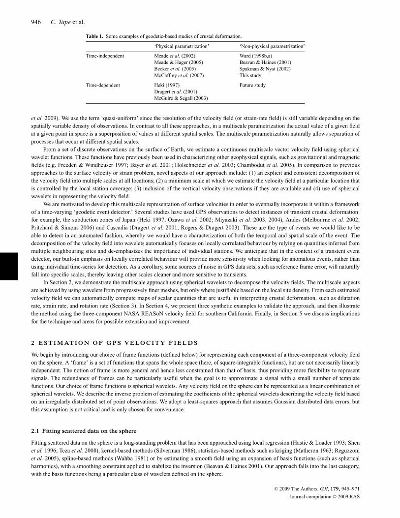
Table 1. Some examples of geodetic-based studies of crustal deformation.

‘Physical parametrization’ ‘Non-physical parametrization’

Time-independent Meade et al. (2002) Ward (1998b,a)Meade & Hager (2005) Beavan & Haines (2001)Becker et al. (2005) Spakman & Nyst (2002)McCaffrey et al. (2007) This study

Time-dependent Heki (1997) Future studyDragert et al. (2001)McGuire & Segall (2003)

et al. 2009). We use the term ‘quasi-uniform’ since the resolution of the velocity field (or strain-rate field) is still variable depending on thespatially variable density of observations. In contrast to all these approaches, in a multiscale parametrization the actual value of a given fieldat a given point in space is a superposition of values at different spatial scales. The multiscale parametrization naturally allows separation ofprocesses that occur at different spatial scales.

From a set of discrete observations on the surface of Earth, we estimate a continuous multiscale vector velocity field using sphericalwavelet functions. These functions have previously been used in characterizing other geophysical signals, such as gravitational and magneticfields (e.g. Freeden & Windheuser 1997; Bayer et al. 2001; Holschneider et al. 2003; Chambodut et al. 2005). In comparison to previousapproaches to the surface velocity or strain problem, novel aspects of our approach include: (1) an explicit and consistent decomposition ofthe velocity field into multiple scales at all locations; (2) a minimum scale at which we estimate the velocity field at a particular location thatis controlled by the local station coverage; (3) inclusion of the vertical velocity observations if they are available and (4) use of sphericalwavelets in representing the velocity field.

We are motivated to develop this multiscale representation of surface velocities in order to eventually incorporate it within a frameworkof a time-varying ‘geodetic event detector.’ Several studies have used GPS observations to detect instances of transient crustal deformation:for example, the subduction zones of Japan (Heki 1997; Ozawa et al. 2002; Miyazaki et al. 2003, 2004), Andes (Melbourne et al. 2002;Pritchard & Simons 2006) and Cascadia (Dragert et al. 2001; Rogers & Dragert 2003). These are the type of events we would like to beable to detect in an automated fashion, whereby we would have a characterization of both the temporal and spatial scale of the event. Thedecomposition of the velocity field into wavelets automatically focuses on locally correlated behaviour by relying on quantities inferred frommultiple neighbouring sites and de-emphasizes the importance of individual stations. We anticipate that in the context of a transient eventdetector, our built-in emphasis on locally correlated behaviour will provide more sensitivity when looking for anomalous events, rather thanusing individual time-series for detection. As a corollary, some sources of noise in GPS data sets, such as reference frame error, will naturallyfall into specific scales, thereby leaving other scales cleaner and more sensitive to transients.

In Section 2, we demonstrate the multiscale approach using spherical wavelets to decompose the velocity fields. The multiscale aspectsare achieved by using wavelets from progressively finer meshes, but only where justifiable based on the local site density. From each estimatedvelocity field we can automatically compute maps of scalar quantities that are useful in interpreting crustal deformation, such as dilatationrate, strain rate, and rotation rate (Section 3). In Section 4, we present three synthetic examples to validate the approach, and then illustratethe method using the three-component NASA REASoN velocity field for southern California. Finally, in Section 5 we discuss implicationsfor the technique and areas for possible extension and improvement.

2 E S T I M AT I O N O F G P S V E L O C I T Y F I E L D S

We begin by introducing our choice of frame functions (defined below) for representing each component of a three-component velocity fieldon the sphere. A ‘frame’ is a set of functions that spans the whole space (here, of square-integrable functions), but are not necessarily linearlyindependent. The notion of frame is more general and hence less constrained than that of basis, thus providing more flexibility to representsignals. The redundancy of frames can be particularly useful when the goal is to approximate a signal with a small number of templatefunctions. Our choice of frame functions is spherical wavelets. Any velocity field on the sphere can be represented as a linear combination ofspherical wavelets. We describe the inverse problem of estimating the coefficients of the spherical wavelets describing the velocity field basedon an irregularly distributed set of point observations. We adopt a least-squares approach that assumes Gaussian distributed data errors, butthis assumption is not critical and is only chosen for convenience.

2.1 Fitting scattered data on the sphere

Fitting scattered data on the sphere is a long-standing problem that has been approached using local regression (Hastie & Loader 1993; Shenet al. 1996; Teza et al. 2008), kernel-based methods (Silverman 1986), statistics-based methods such as kriging (Matheron 1963; Reguzzoniet al. 2005), spline-based methods (Wahba 1981) or by estimating a smooth field using an expansion of basis functions (such as sphericalharmonics), with a smoothing constraint applied to stabilize the inversion (Beavan & Haines 2001). Our approach falls into the last category,with the basis functions being a particular class of wavelets defined on the sphere.

C© 2009 The Authors, GJI, 179, 945–971

Journal compilation C© 2009 RAS

Multiscale estimation of GPS velocity fields 947

We denote the time-dependent position of the ith GPS station in a network by xi (t), whose origin is that of an external reference frame(e.g. ITRF2005 or fixed North America). Over an interval of time, �t , the station moves �xi , and thus the velocity of the station over thisinterval is vi = �xi/�t .

A velocity field defined on a sphere of radius R can be written as

v(θ, φ) = vr (θ, φ) r + vθ (θ, φ) θ + vφ(θ, φ) φ, (1)

where r is the vertical direction, θ is the south direction and φ is the east direction. Our goal is to estimate the field v(θ , φ) from a set ofmeasurements taken at N irregularly distributed stations, with coordinates (θi , φi ), i = 1, . . . , N . These measurements, denoted by

vi = (vir , vi

θ , viφ

)(2)

= [vr (θi , φi ), vθ (θi , φi ), vφ(θi , φi )] (3)

are assumed to be contaminated by noise. We are interested in functional descriptions of the field v(θ , φ) having the capability to adapt thescale locally in relation to the local density of the GPS stations. These descriptions should also allow decoupling of the velocity field atdifferent spatial scales, since they may be associated with different physical phenomena or different sources of noise.

2.1.1 Wavelets on the sphere

Our desire to efficiently distinguish between multiple phenomena and noise sources that may be present in a given data set motivates the useof a spatio-spectral (or multiscale) representation (e.g. Simons & Hager 1997; Simons et al. 1997). Wavelets provide a natural representationfor such multiscale signals. The formal extension of wavelet analysis to a spherical manifold has been an active research field in the last15 yr (Dahlke & Maass 1996; Freeden & Windheuser 1996, 1997; Holschneider 1996; Simons & Hager 1997; Antoine & Vandergheynst1999; Bogdanova et al. 2005; Wiaux et al. 2005). Applications in geophysics include analyses of Earth’s magnetic field and gravity field(Holschneider et al. 2003; Chambodut et al. 2005). An application to the global temperature field is presented in Oh & Li (2004).

In order to define a wavelet analysis in the space L2(S2) of square-integrable functions on the unit sphere, two basic operations arerequired: rotations (which play the role of translations in the Euclidean case), and dilatations. The major difficulty in deriving wavelets onthe sphere lies in the definition of a proper dilatation operator, directly linked in wavelet theory to the notion of scale. Here we follow theapproach proposed by Antoine & Vandergheynst (1999), whereby continuous spherical wavelets are derived from Euclidean wavelets byinverse stereographic projection. An alternative would be to use spherical wavelets constructed from spherical harmonics (e.g. Holschneideret al. 2003; Simons et al. 2006; Guilloux et al. 2009).

Bogdanova et al. (2005) proved that the inverse stereographic projection of any admissible 2-D wavelet in R2 yields an admissible

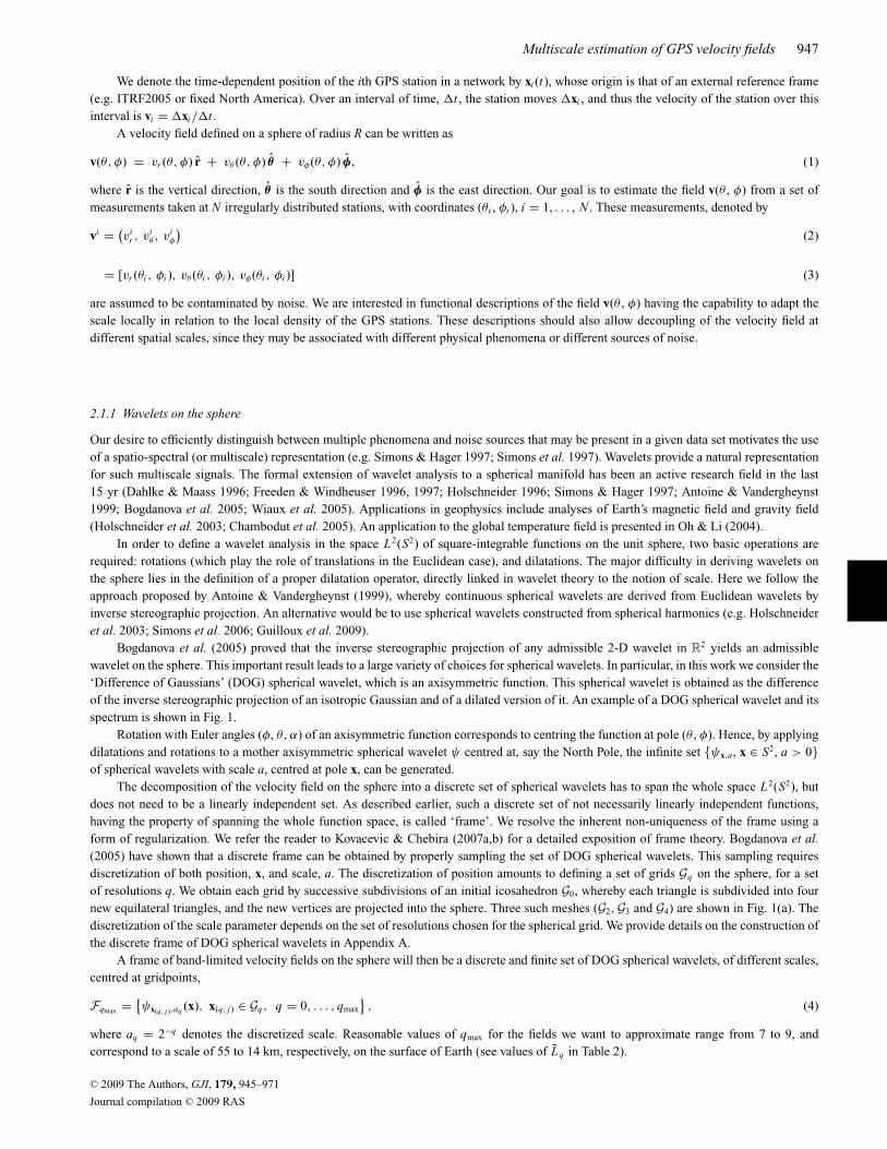
wavelet on the sphere. This important result leads to a large variety of choices for spherical wavelets. In particular, in this work we consider the‘Difference of Gaussians’ (DOG) spherical wavelet, which is an axisymmetric function. This spherical wavelet is obtained as the differenceof the inverse stereographic projection of an isotropic Gaussian and of a dilated version of it. An example of a DOG spherical wavelet and itsspectrum is shown in Fig. 1.

Rotation with Euler angles (φ, θ , α) of an axisymmetric function corresponds to centring the function at pole (θ , φ). Hence, by applyingdilatations and rotations to a mother axisymmetric spherical wavelet ψ centred at, say the North Pole, the infinite set {ψx,a, x ∈ S2, a > 0}of spherical wavelets with scale a, centred at pole x, can be generated.

The decomposition of the velocity field on the sphere into a discrete set of spherical wavelets has to span the whole space L2(S2), butdoes not need to be a linearly independent set. As described earlier, such a discrete set of not necessarily linearly independent functions,having the property of spanning the whole function space, is called ‘frame’. We resolve the inherent non-uniqueness of the frame using aform of regularization. We refer the reader to Kovacevic & Chebira (2007a,b) for a detailed exposition of frame theory. Bogdanova et al.(2005) have shown that a discrete frame can be obtained by properly sampling the set of DOG spherical wavelets. This sampling requiresdiscretization of both position, x, and scale, a. The discretization of position amounts to defining a set of grids Gq on the sphere, for a setof resolutions q. We obtain each grid by successive subdivisions of an initial icosahedron G0, whereby each triangle is subdivided into fournew equilateral triangles, and the new vertices are projected into the sphere. Three such meshes (G2,G3 and G4) are shown in Fig. 1(a). Thediscretization of the scale parameter depends on the set of resolutions chosen for the spherical grid. We provide details on the construction ofthe discrete frame of DOG spherical wavelets in Appendix A.

A frame of band-limited velocity fields on the sphere will then be a discrete and finite set of DOG spherical wavelets, of different scales,centred at gridpoints,

Fqmax = {ψx(q, j),aq (x), x(q, j) ∈ Gq , q = 0, . . . , qmax

}, (4)

where aq = 2−q denotes the discretized scale. Reasonable values of qmax for the fields we want to approximate range from 7 to 9, andcorrespond to a scale of 55 to 14 km, respectively, on the surface of Earth (see values of Lq in Table 2).

C© 2009 The Authors, GJI, 179, 945–971


948 C. Tape et al.

Figure 1. Spherical wavelet frame functions. (a) Triangulated spherical grids used for determining the locations for the centres of the spherical wavelet framefunctions. From left- to right-hand side are grids for orders q = 2 (162 vertices), q = 3 (642 vertices) and q = 4 (2562 vertices) (Table 2). (b) Three differentscales of a DOG (Difference of Gaussian) spherical wavelet centred at the North Pole. (c) Corresponding profiles of wavelets in (b), for a fixed longitude φ.(d) Corresponding spectra of wavelets in (b).

2.2 Decomposition of the velocity field in spherical wavelets

For the sake of clarity, we assume from now on that an ordering on the elements of Fqmax has been established, and we write Fqmax ={gk(x), k = 1, . . . , M}. Any scalar function f ∈ L2(S2) whose bandwidth does not exceed the one associated to the finest scale qmax can bewritten as

f (x) =M∑

k=1

mk gk(x) = gT (x) m. (5)

C© 2009 The Authors, GJI, 179, 945–971



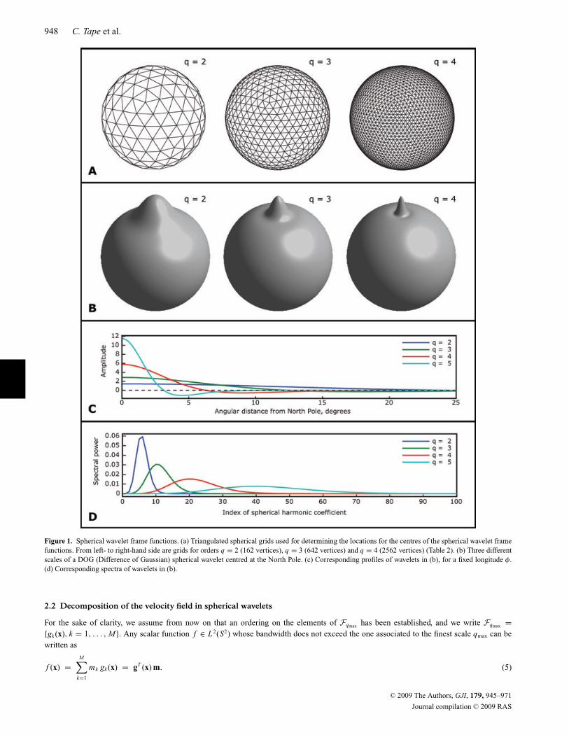
Table 2. Geometric properties of the spherical-triangular grids, after Wang & Dahlen (1995).

Average side Max. representableOrder, q Faces, Fq Vertices, Vq arc-length,a Lq bandwidth, lq

0 20 12 63.435◦ 7053.64 km 31 80 42 31.718◦ 3526.82 km 62 320 162 15.859◦ 1763.41 km 113 1 280 642 7.929◦ 881.71 km 234 5 120 2 562 3.965◦ 440.85 km 455 20 480 10 242 1.982◦ 220.43 km 916 81 920 40 962 0.991◦ 110.21 km 1827 327 680 163 842 0.496◦ 55.11 km 3638 1310 720 655 362 0.248◦ 27.55 km 7269 5242 880 2621 442 0.124◦ 13.78 km 145310 20 971 520 10 485 762 0.062◦ 6.89 km 290611 83 886 080 41 943 042 0.031◦ 3.44 km 581112 335 544 320 167 772 162 0.016◦ 1.72 km 11 623

q Fq = 20 × 4q Vq = 10 × 4q + 2 Lq = 2−q L0 lq = int(π/Lq )

a L0 = cos−1{cos(72◦)/[1 − cos(72◦)]} ≈ 1.1071 ≈ 63.43◦.

Since the frame Fqmax is not an orthogonal basis, the problem of finding optimal coefficients mk is underdetermined and the solution isnot unique. However, by including some form of regularization, a unique optimal representation can be found. We discuss the issue ofregularization in more detail in the next section. The velocity vector field approximation problem can be reduced to three scalar estimationproblems. If each of the three components is square-integrable, with bandwidth smaller than lqmax , we can then write

v(θ, φ) =M∑

k=1

[ak gk(θ, φ)r(θ, φ) + bk gk(θ, φ) θ (θ, φ) + ck gk(θ, φ) φ(θ, φ)]. (6)

The evaluation of (6) at the observation sites (θi , φi ), i = 1, . . . , N (to which the noisy measurements (vir, v

iθ , vi

φ) have been associated), leadsto

vir =

M∑k=1

ak gk(θi , φi ) + nir , vi

θ =M∑

k=1

bk gk(θi , φi ) + niθ , vi

φ =M∑

k=1

ck gk(θi , φi ) + niφ , (7)

where nir, ni

θ and niφ denote the measurement noise. Consequently, in the following we consider the estimation of a generic spherical scalar

field f (x) from N irregularly distributed sample points xi , i = 1, . . . , N

fi = f (xi ) = gT (xi ) m + ni . (8)

Eq. (8) can be written in matrix form as

f = G m + n, (9)

where f ∈ RN is the vector of measurements, G ∈ R

N×M is the design matrix with Gik = gk(xi ) and m ∈ RM is the model parameter vector.

2.3 The inverse problem, including uncertainties and regularization

We estimate the model vector, m, by minimizing the regularized least-squares functional

F(m) = 1

2(Gm − d)T C−1

D (Gm − d) + 1

2λ2mT Sm. (10)

The observations are assumed to be contaminated by a Gaussian noise of zero mean and data covariance matrix CD. Each diagonal elementof the data covariance matrix is the variance associated with each observation. Thus, the first term in (10) is the data misfit, and the secondterm is the model regularization, with regularization parameter λ.

Typical choices of regularization for when model m represents a spatial quantity include the norm of the model, the norm of the modelgradient, or the Laplacian of the model. In our case, we regularize according to the norm of the gradient of the estimated model. The

C© 2009 The Authors, GJI, 179, 945–971


950 C. Tape et al.

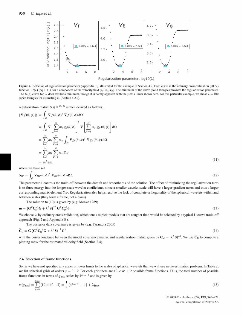
Figure 2. Selection of regularization parameter (Appendix B), illustrated for the example in Section 4.2. Each curve is the ordinary cross-validation (OCV)function, H (λ) (eq. B11), for a component of the velocity field (vr , vθ , vφ ). The minimum of the curve (solid triangle) provides the regularization parameter.The H (λ) curve for vr does exhibit a minimum, though it is barely apparent with the y-axis limits shown here. For this particular example, we chose λ = 100(open triangle) for estimating vr (Section 4.2.2).

regularization matrix S ∈ RM×M is then derived as follows:

‖∇ f (θ, φ)‖22 =

∫S2

∇ f (θ, φ)T ∇ f (θ, φ) d

=∫

S2∇[

M∑k=1

mk gk(θ, φ)

]T

∇[

M∑k′=1

mk′ gk′ (θ, φ)

]d

=M∑

k=1

mk

M∑k′=1

mk′

∫S2

∇gk(θ, φ)T ∇gk′ (θ, φ) d

=M∑

k=1

mk

M∑k′=1

mk′ Skk′

= mT Sm,(11)

where we have set

Skk′ =∫

S2∇gk(θ, φ)T ∇gk′ (θ, φ) d. (12)

The parameter λ controls the trade-off between the data fit and smoothness of the solution. The effect of minimizing the regularization termis to force energy into the longer-scale wavelet coefficients, since a smaller wavelet scale will have a larger gradient norm and thus a largercorresponding matrix element Skk′ . Regularization also helps resolve the lack of complete orthogonality of the spherical wavelets within andbetween scales (they form a frame, not a basis).

The solution to (10) is given by (e.g. Menke 1989)

m = (GT C−1D G + λ2 S

)−1GT C−1

D d. (13)

We choose λ by ordinary cross-validation, which tends to pick models that are rougher than would be selected by a typical L-curve trade-offapproach (Fig. 2 and Appendix B).

The posterior data covariance is given by (e.g. Tarantola 2005)

CD = G(GT C−1

D G + λ2 S)−1

GT , (14)

with the correspondence between the model covariance matrix and regularization matrix given by CM = (λ2 S)−1. We use CD to compute aplotting mask for the estimated velocity field (Section 2.4).

2.4 Selection of frame functions

So far we have not specified any upper or lower limits to the scales of spherical wavelets that we will use in the estimation problem. In Table 2,we list spherical grids of orders q = 0–12. For each grid there are 10 × 4q + 2 possible frame functions. Thus, the total number of possibleframe functions in terms of qmax scales by 4qmax+1 and is given by

m(qmax) =qmax∑q=0

[10 × 4q + 2] = 1

3

(4qmax+1 − 1

)+ 2qmax, (15)

C© 2009 The Authors, GJI, 179, 945–971



Table 3. Spectral and spatial support of spherical wavelets.

Scale Spatial support Spectral supportq aq 0.990‖ψa‖2

0 20 82.442◦ 9167.1 km 41 2−1 47.310◦ 5260.7 km 62 2−2 24.707◦ 2747.3 km 103 2−3 12.500◦ 1389.9 km 204 2−4 6.268◦ 697.0 km 415 2−5 3.136◦ 348.8 km 836 2−6 1.569◦ 174.4 km 1667 2−7 0.784◦ 87.2 km 3328 2−8 0.392◦ 43.6 km 6659 2−9 0.196◦ 21.8 km 1329

Notes: Spatial support is defined as the distance to the firstzero-crossing (see Fig. 1c). Spectral support is computed as thespherical harmonic degrees at which the energy reaches 99.0 per centof the total energy (see Fig. 1d).

Figure 3. Selection of spherical wavelets based on the REASoN observation points, using scales q = 3–12. The density of the observation points, plotted asinverted triangles, controls the selection of spherical wavelets, whose centre points are not shown. The colour map shows the maximum-q scale wavelet that‘covers’ each area, where the coverage is determined by the length scale for each spherical wavelet (Table 3). Where stations are dense, wavelets with all scalesq = 3–12 (red) are available; where stations are sparse, only wavelets with long length scales q = 3–6 (blue) are available.

where we have used the formula for summing a geometric series. With no computational restrictions and careful choice of regularization, it ispossible to use all available frame functions for every grid. However, for computational and practical purposes, it is desirable to use a reducedset of frame functions. Our algorithm first eliminates frame functions that have fewer than three stations within their ‘footprint,’ defined(somewhat arbitrarily) as the region inside the first zero-crossing of the spherical wavelet (Table 3). This procedure thereby determines therange of allowable q-values based on the local density of stations. An example is shown in Fig. 3 based on the REASoN stations in southernCalifornia; the density of stations allows for qmax = 12. One may also choose to choose a qmax that is less than what is permitted by the stationdensity; this choice will stabilize the estimation problem and reduce the possibility of overfitting the observations. We have chosen qmax ≤ 9for each example in Section 4.

We also restrict qmin based on the approximate outer length scale, L, of the network. We select qmin such that the support of the qmin

wavelets is less than 2L . This restriction is not required, since proper regularization should leave little power in wavelets that are much largerthan the network, and we already remove a pure rotational field, as described next.

C© 2009 The Authors, GJI, 179, 945–971


952 C. Tape et al.

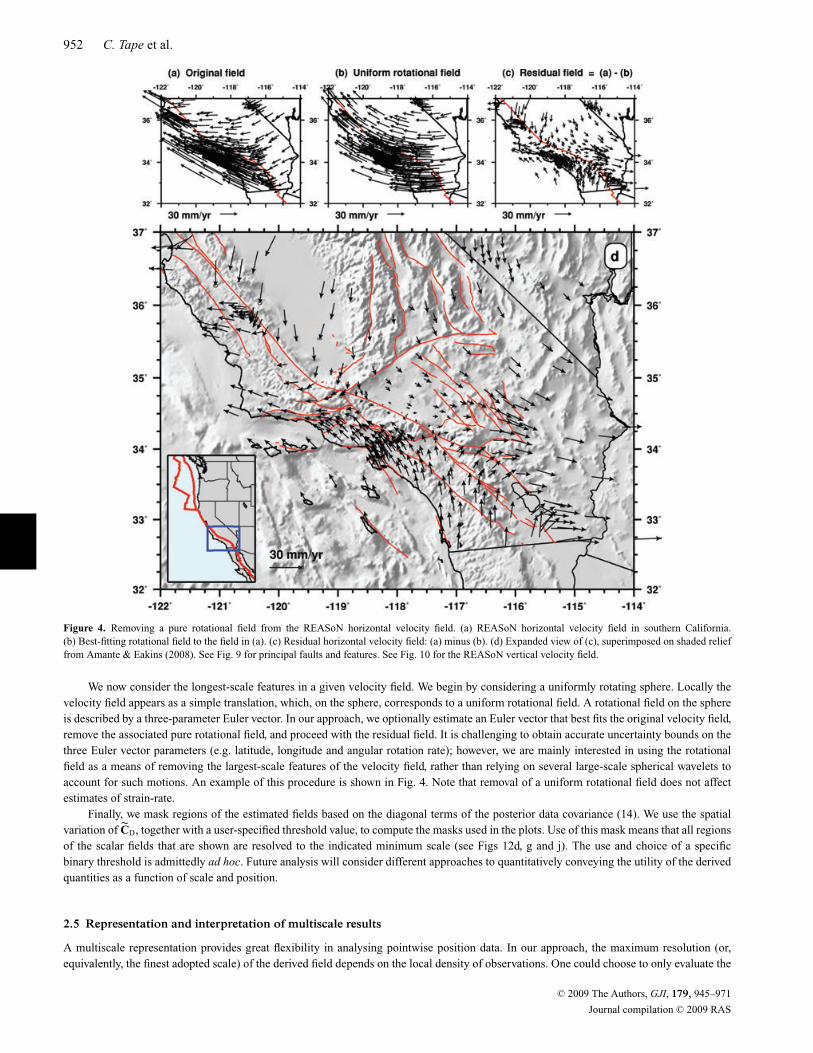
Figure 4. Removing a pure rotational field from the REASoN horizontal velocity field. (a) REASoN horizontal velocity field in southern California.(b) Best-fitting rotational field to the field in (a). (c) Residual horizontal velocity field: (a) minus (b). (d) Expanded view of (c), superimposed on shaded relieffrom Amante & Eakins (2008). See Fig. 9 for principal faults and features. See Fig. 10 for the REASoN vertical velocity field.

We now consider the longest-scale features in a given velocity field. We begin by considering a uniformly rotating sphere. Locally thevelocity field appears as a simple translation, which, on the sphere, corresponds to a uniform rotational field. A rotational field on the sphereis described by a three-parameter Euler vector. In our approach, we optionally estimate an Euler vector that best fits the original velocity field,remove the associated pure rotational field, and proceed with the residual field. It is challenging to obtain accurate uncertainty bounds on thethree Euler vector parameters (e.g. latitude, longitude and angular rotation rate); however, we are mainly interested in using the rotationalfield as a means of removing the largest-scale features of the velocity field, rather than relying on several large-scale spherical wavelets toaccount for such motions. An example of this procedure is shown in Fig. 4. Note that removal of a uniform rotational field does not affectestimates of strain-rate.

Finally, we mask regions of the estimated fields based on the diagonal terms of the posterior data covariance (14). We use the spatialvariation of CD, together with a user-specified threshold value, to compute the masks used in the plots. Use of this mask means that all regionsof the scalar fields that are shown are resolved to the indicated minimum scale (see Figs 12d, g and j). The use and choice of a specificbinary threshold is admittedly ad hoc. Future analysis will consider different approaches to quantitatively conveying the utility of the derivedquantities as a function of scale and position.

2.5 Representation and interpretation of multiscale results

A multiscale representation provides great flexibility in analysing pointwise position data. In our approach, the maximum resolution (or,equivalently, the finest adopted scale) of the derived field depends on the local density of observations. One could choose to only evaluate the

C© 2009 The Authors, GJI, 179, 945–971



velocity field at scales that are allowable everywhere, in other words, the maximum value of the smallest scale allowed by a given networkconfiguration. This choice would unnecessarily limit the detail of the resultant field. An alternative approach is to construct a single velocityfield where the scale of information represented by the field varies as a function position in a given spatially heterogeneous network ofobservations. This approach may be useful for generating velocity field maps that are spatially uninterrupted, but is dangerous because itencourages the comparisons of derived quantities (such as strain rates) evaluated at different scales, thereby allowing one to spuriously inferspatial variability where none exists. In this study, we resist the temptation to produce a single map but insist on a perspective that considersscales of deformation separately, or at most, sums up all resolvable scales, but through error-based spatial masks, only allows for comparisonof regions that are comparable at a given spatial resolution.

In the future, one might compare our estimates of strain-rate-like quantities with those from physical models (e.g. Meade & Hager2005). Given that our estimates are essentially filtered versions of a true underlying field, such comparisons should be made by taking modelpredictions of velocities evaluated at the same points as the observed data and then estimating any derived quantities using the same approach(including the same value of regularization) that was used when treating the observed data (e.g. Simons et al. 1997).

3 S T R A I N R AT E M A P S A N D O T H E R S C A L A R Q UA N T I T I E S

A vector and tensor are physical quantities. However, in practice we choose a basis (or coordinate system, e.g. r−θ−φ) to describe them. Oncea basis is chosen, we can discuss the components of a vector (e.g. vr , vθ , vφ) or tensor. The norm of a vector or tensor does not depend onthe choice of basis, but it does depend on the choice of reference frame (for example, what is taken to be fixed). The norm of the gradient ofthe velocity field does not depend on the choice of basis or the reference frame. In this section, we examine what kinds of scalar quantitiesare sensible to derive from tensor quantities. Maps of these scalar quantities illuminate regions of deformation that may be difficult to detectfrom a visual inspection of the estimated velocity field.

Many different scalar quantities have been used in previous studies. Here we list several of these, assuming that the strain-rate tensor, D(e.g. eq. 16), is 3 × 3 and has eigenvalues λ1, λ2 and λ3, with λ1 ≥ λ2 ≥ λ3. For simplicity, we leave out multiplicative constants.

(i) λ1 + λ2 + λ3 (e.g. Ward 1998b; Beavan & Haines 2001), equal to the trace of D.(ii) max [ |λ1| |λ2| |λ3| ] (Ward 1998b).(iii)

√D : D (see eq. D5) (Bos et al. 2003).

(iv)√

D : D, but ignoring components of D associated with r:√

D2φφ + D2

θθ + 2D2φθ (Kreemer et al. 2003).

(v) | λ1 − λ3 | (Beavan & Haines 2001).(vi) Drθ , Drφ , or Dθφ (Flesch et al. 2005).(vii) Wθφ (Allmendinger et al. 2007), an element of the rotation tensor W (e.g. eq. 17).

Other more complicated expressions have also been used (e.g. Holt et al. 2000, eq. 14). We prefer to use scalar quantities that are invariantunder coordinate transformations (Section 3.2). Because the eigenvalues do not depend on the choice of coordinate system, any scalar functionin terms of eigenvalues is also an invariant quantity.

3.1 The velocity gradient tensor

Once we have computed the estimated velocity field, v(θ , φ), we can readily compute its surface derivatives and other tensor and scalarquantities. The spatial velocity gradient, L, is defined by

L ≡ (∇v)T = v∇,

and can be decomposed as L = D + W, where D is symmetric and W is antisymmetric. For a 3-D velocity field, these expressions are†

D = 1

2(L + LT ) =

⎡⎢⎢⎢⎢⎣∂vr∂r

12r

(−vθ + ∂vr∂θ

+ r ∂vθ

∂r

)12r

(−vφ + 1

sin θ

∂vr∂φ

+ r∂vφ

∂r

)D12

1r

(vr + ∂vθ

∂θ

)12r

(−vφ cot θ + 1

sin θ

∂vθ

∂φ+ ∂vφ

∂θ

)D13 D23

1r

(vr + vθ cot θ + 1

sin θ

∂vφ

∂φ

)⎤⎥⎥⎥⎥⎦ , (16)

W = 1

2

(L − LT

) =

⎡⎢⎢⎢⎣0 1

2r


− r ∂vθ

∂r

)12r

(−vφ + 1

sin θ

∂vr∂φ

− r∂vφ

∂r

)−W12 0 1

2r

(−vφ cot θ + 1

sin θ

∂vθ

∂φ− ∂vφ

∂θ

)−W13 −W23 0

⎤⎥⎥⎥⎦ . (17)

Physically speaking, D is the strain-rate tensor and W is the rotation-rate tensor, though typically this terminology is reserved for thecondition of ‘small’ deformation, where Di j 1 and Wi j 1 (Malvern 1969, pp. 148–150). For the examples in Section 4, Di j and Wi j aretypically less than 10−7.

† These can be found in Malvern (1969, p. 671), though note the cos φ typo (instead of cos θ ) in his expression for Dθφ .

C© 2009 The Authors, GJI, 179, 945–971


954 C. Tape et al.

3.1.1 Some practical reductions for simple rheologies

With observations only at the surface, we do not have access to vertical derivatives of the velocity field, ∂vr/∂r , ∂vr/∂θ , and ∂vr/∂φ.Furthermore, in many scenarios the vertical component of the velocity field (vr ) and its horizontal derivatives (∂vr/∂θ , ∂vr/∂φ) are notavailable. However, these observational limitations do not mean that L, D and W reduce to 2 × 2 tensors, even if one assumes that the missingquantities are equal to zero, because Drθ contains vθ , and Drφ contains vφ . To eliminate some of the unknown terms, we can use the fact thatwe are observing at the free-surface (i.e. zero tractions) in combination with simple assumptions regarding the rheological behaviour that isdominant at the surface on the timescale of the observations. We first assume a spherical Earth, ignoring both ellipticity and topography, thatis, ignoring any deviations of the free surface from r = R. The free surface condition then becomes

σ r = 0, (18)

where σ is the second-order symmetric stress tensor, and r = (1, 0, 0) is the upward-pointing unit normal in r−θ−φ local coordinates.Eq. (18) provides the constraints

σ11 = 0, σ21 = σ12 = 0, σ31 = σ13 = 0. (19)

For both simple isotropic viscous and isotropic elastic rheologies, then D21 = D12 = 0 and D31 = D13 = 0. If we assume a linear elasticrheology, then for observations at the surface, eqs (16) and (17) reduce to (see Appendix C)

Delastic0 =

⎡⎢⎢⎢⎣F (D22 + D33) 0 0

0 1R

(vr + ∂vθ

∂θ

)1

2R

(−vφ cot θ + 1

sin θ

∂vθ

∂φ+ ∂vφ

∂θ

)0 D23

1R


sin θ

∂vφ

∂φ

)⎤⎥⎥⎥⎦ , (20)

Welastic0 =

⎡⎢⎢⎢⎣0 1

R


)1R

(−vφ + 1

sin θ

∂vr∂φ

)−W12 0 1

2R

(−vφ cot θ + 1

sin θ

∂vθ

∂φ− ∂vφ

∂θ

)−W13 −W23 0

⎤⎥⎥⎥⎦ , (21)

where

F = −λ / (λ + 2μ) (22)

is a constant, and λ and μ are Lame parameters. For a Poisson solid, λ = μ, and F = −1/3.We now assume a linear viscous rheology of the form (Malvern 1969, p. 298)

σ = Tr(σ )I + � Tr(D)I + 2ηD , (23)

where η and � characterize the viscosity. With the assumption of incompressibility, ∇ · v = Tr (L) = Tr (D) = 0, we obtain the constraintD11 = −(D22 + D33). In comparison with eq. (20), this corresponds to F = −1. Applying the free-surface constraints in eq. (19), we obtainthe additional constraints, D12 = D13 = 0, and the algebra follows the elastic case, but with F = −1.

3.2 Scalar quantities derived from tensors

In our examples, we consider three invariant quantities, related to dilatation rate (�), strain rate (�) and rotation rate (). In functional form,these quantities are written as �(θ , φ), �(θ , φ) and (θ , φ), since our observations are restricted to the surface of the sphere.

3.2.1 Dilatation rate

The dilatation rate, or volumetric strain rate, is the divergence of the velocity field, or, equivalently, the first invariant of the velocity gradienttensor

� ≡ ∇ · v = Tr(L) = Tr(D)

= r−1

[2 vr + vθ cot θ + r

∂vr

∂r+ ∂vθ

∂θ+ 1

sin θ

∂vφ

∂φ

], (24)

listed in Malvern (1969, p. 670). The dilatation rate, after applying the free-surface condition, is obtained from eq. (20)

�elastic0 = 1

R(F + 1)

(2 vr + vθ cot θ + ∂vθ

∂θ+ 1

sin θ

∂vφ

∂φ

), (25)

which is used in the examples in Section 4.

C© 2009 The Authors, GJI, 179, 945–971



3.2.2 Strain rate

We define a strain-rate quantity, �, to be the Frobenius norm (Appendix D) of the strain-rate tensor D. Mathematically, � can be expressedas (Appendix D)

� = ‖D‖F =√

D : D =√

tr (DD) , (26)

which is used in Bos et al. (2003). For the remainder of this paper, we will abbreviate ‘Frobenius norm of the strain-rate tensor’ as ‘strainrate.’

3.2.3 Rotation rate

The rotation vector, w = 12 ∇ × v, is determined from the components of the rotation-rate tensor, W, as (Malvern 1969, p. 147)

w = −Wθφ r + Wrφ θ − Wrθ φ. (27)

Substituting the terms in eq. (21), we obtain

w = 1

2R

(vφ cot θ − 1

sin θ

∂vθ

∂φ+ ∂vφ

∂θ

)r + 1

R

(−vφ + 1

sin θ

∂vr

∂φ

)θ + 1

R

(vθ − ∂vr

∂θ

)φ, (28)

which is the rotation vector associated with a point on the surface of the sphere, (R, θ , φ). The magnitude of rotation is

≡ |w| = (W 2θφ + W 2

φr + W 2rθ

)1/2. (29)

The units of should be radians per unit time. This quantity is invariant under coordinate transformations; it can also be expressed as(Appendix D)

= 1√2

‖W‖F =√

−1

2Tr(WW) =

√1

2W : W. (30)

The location of the rotation pole is the (longitude, latitude) where the unit vector w/|w| intersects the sphere.For physical interpretations, we partition the rotation vector (eq. 28) into two vectors, w = ws + wt, where

ws = 1

2R

(vφ cot θ − 1

sin θ

∂vθ

∂φ+ ∂vφ

∂θ

)r − vφ

Rθ + vθ

Rφ, (31)

wt = 1

R

(1

sin θ

∂vr

∂φ

)θ + 1

R

(∂vr

∂θ

)φ. (32)

The subscript ‘s’ is applied to denote ‘sphere,’ in that all velocity terms are tangential to the surface of the sphere (vθ and vφ); the subscript‘t’ is applied to denote ‘tilt,’ in that all terms are related to local tilt-like motion.

3.3 Linear scalar quantities

The tensors L, D and W—and the rotation vector w—are all linear with respect to decompositions of v into different scales. However, of thethree scalar quantities discussed above—dilatation rate (�), strain rate (�) and rotation rate ()—only dilatation rate is linear with respect todecompositions of v. For example, if we decompose v into five subfields, then the sum of the dilatation rates of the subfields is equal to thedilatation of v. The strain rate quantity is not linear because of the squared terms in eq. (26). The rotation rate quantity is not linear becauseof the squared terms in eq. (29).

4 E X A M P L E S

Here we present a series of examples illustrating the multiscale estimation technique described in Section 2. For the computations of thevelocity gradient, we employ the free-surface condition and assume a linear elastic rheology, as summarized in Appendix C, with the keyformulas eqs (20) and (21). The scales used in each example are summarized in Table 2: low q refers to long length scales, while high q refersto short length scales.

As previously described, spherical wavelets are automatically selected based on station density, and optionally, a user-defined qmax

(Section 2.4 and Fig. 3). In estimating the coefficients for each wavelet, a regularization parameter is obtained using ordinary cross-validation(Appendix B and Fig. 2).

4.1 Synthetic examples

Results from three synthetic examples are shown in Figs 5–8. Most of the synthetic fields do not have any direct relevance to southernCalifornia; we use them only to highlight different styles of deformation that could be observed in a tectonic setting.

C© 2009 The Authors, GJI, 179, 945–971


956 C. Tape et al.

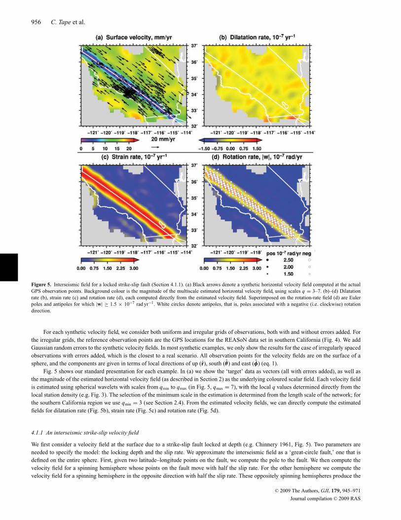
Figure 5. Interseismic field for a locked strike-slip fault (Section 4.1.1). (a) Black arrows denote a synthetic horizontal velocity field computed at the actualGPS observation points. Background colour is the magnitude of the multiscale estimated horizontal velocity field, using scales q = 3–7. (b)–(d) Dilatationrate (b), strain rate (c) and rotation rate (d), each computed directly from the estimated velocity field. Superimposed on the rotation-rate field (d) are Eulerpoles and antipoles for which |w| ≥ 1.5 × 10−7 rad yr−1. White circles denote antipoles, that is, poles associated with a negative (i.e. clockwise) rotationdirection.

For each synthetic velocity field, we consider both uniform and irregular grids of observations, both with and without errors added. Forthe irregular grids, the reference observation points are the GPS locations for the REASoN data set in southern California (Fig. 4). We addGaussian random errors to the synthetic velocity fields. In most synthetic examples, we only show the results for the case of irregularly spacedobservations with errors added, which is the closest to a real scenario. All observation points for the velocity fields are on the surface of asphere, and the components are given in terms of local directions of up (r), south (θ ) and east (φ) (eq. 1).

Fig. 5 shows our standard presentation for each example. In (a) we show the ‘target’ data as vectors (all with errors added), as well asthe magnitude of the estimated horizontal velocity field (as described in Section 2) as the underlying coloured scalar field. Each velocity fieldis estimated using spherical wavelets with scales from qmin to qmax (in Fig. 5, qmax = 7), with the local q values determined directly from thelocal station density (e.g. Fig. 3). The selection of the minimum scale in the estimation is determined from the length scale of the network; forthe southern California region we use qmin = 3 (see Section 2.4). From the estimated velocity fields, we can directly compute the estimatedfields for dilatation rate (Fig. 5b), strain rate (Fig. 5c) and rotation rate (Fig. 5d).

4.1.1 An interseismic strike-slip velocity field

We first consider a velocity field at the surface due to a strike-slip fault locked at depth (e.g. Chinnery 1961, Fig. 5). Two parameters areneeded to specify the model: the locking depth and the slip rate. We approximate the interseismic field as a ‘great-circle fault,’ one that isdefined on the entire sphere. First, given two latitude–longitude points on the fault, we compute the pole to the fault. We then compute thevelocity field for a spinning hemisphere whose points on the fault move with half the slip rate. For the other hemisphere we compute thevelocity field for a spinning hemisphere in the opposite direction with half the slip rate. These oppositely spinning hemispheres produce the

C© 2009 The Authors, GJI, 179, 945–971



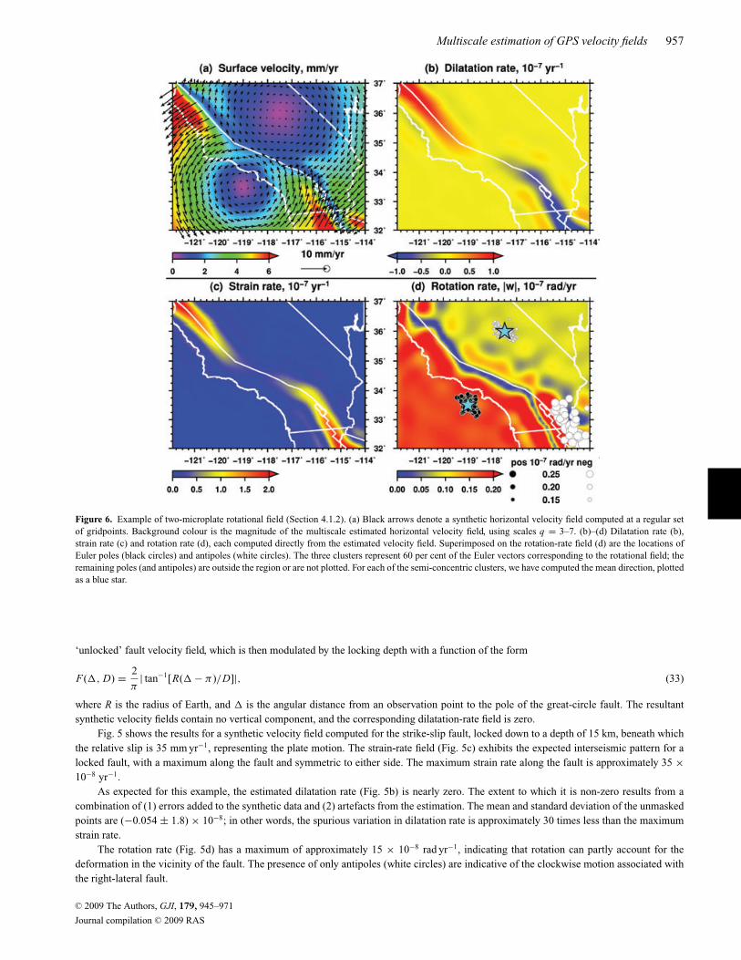
Figure 6. Example of two-microplate rotational field (Section 4.1.2). (a) Black arrows denote a synthetic horizontal velocity field computed at a regular setof gridpoints. Background colour is the magnitude of the multiscale estimated horizontal velocity field, using scales q = 3–7. (b)–(d) Dilatation rate (b),strain rate (c) and rotation rate (d), each computed directly from the estimated velocity field. Superimposed on the rotation-rate field (d) are the locations ofEuler poles (black circles) and antipoles (white circles). The three clusters represent 60 per cent of the Euler vectors corresponding to the rotational field; theremaining poles (and antipoles) are outside the region or are not plotted. For each of the semi-concentric clusters, we have computed the mean direction, plottedas a blue star.

‘unlocked’ fault velocity field, which is then modulated by the locking depth with a function of the form

F(�, D) = 2

π| tan−1[R(� − π )/D]|, (33)

where R is the radius of Earth, and � is the angular distance from an observation point to the pole of the great-circle fault. The resultantsynthetic velocity fields contain no vertical component, and the corresponding dilatation-rate field is zero.

Fig. 5 shows the results for a synthetic velocity field computed for the strike-slip fault, locked down to a depth of 15 km, beneath whichthe relative slip is 35 mm yr−1, representing the plate motion. The strain-rate field (Fig. 5c) exhibits the expected interseismic pattern for alocked fault, with a maximum along the fault and symmetric to either side. The maximum strain rate along the fault is approximately 35 ×10−8 yr−1.

As expected for this example, the estimated dilatation rate (Fig. 5b) is nearly zero. The extent to which it is non-zero results from acombination of (1) errors added to the synthetic data and (2) artefacts from the estimation. The mean and standard deviation of the unmaskedpoints are (−0.054 ± 1.8) × 10−8; in other words, the spurious variation in dilatation rate is approximately 30 times less than the maximumstrain rate.

The rotation rate (Fig. 5d) has a maximum of approximately 15 × 10−8 rad yr−1, indicating that rotation can partly account for thedeformation in the vicinity of the fault. The presence of only antipoles (white circles) are indicative of the clockwise motion associated withthe right-lateral fault.

C© 2009 The Authors, GJI, 179, 945–971


958 C. Tape et al.

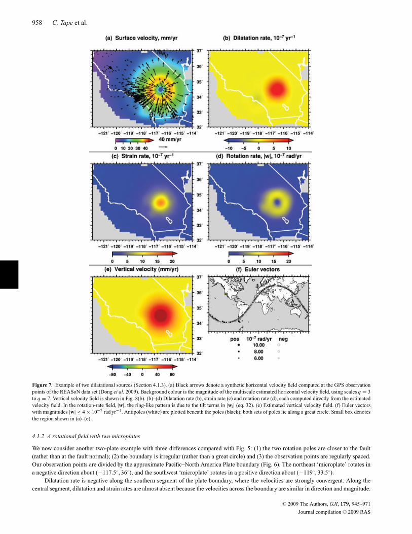
Figure 7. Example of two dilatational sources (Section 4.1.3). (a) Black arrows denote a synthetic horizontal velocity field computed at the GPS observationpoints of the REASoN data set (Dong et al. 2009). Background colour is the magnitude of the multiscale estimated horizontal velocity field, using scales q = 3to q = 7. Vertical velocity field is shown in Fig. 8(b). (b)–(d) Dilatation rate (b), strain rate (c) and rotation rate (d), each computed directly from the estimatedvelocity field. In the rotation-rate field, |w|, the ring-like pattern is due to the tilt terms in |wt| (eq. 32). (e) Estimated vertical velocity field. (f) Euler vectorswith magnitudes |w| ≥ 4 × 10−7 rad yr−1. Antipoles (white) are plotted beneath the poles (black); both sets of poles lie along a great circle. Small box denotesthe region shown in (a)–(e).

4.1.2 A rotational field with two microplates

We now consider another two-plate example with three differences compared with Fig. 5: (1) the two rotation poles are closer to the fault(rather than at the fault normal); (2) the boundary is irregular (rather than a great circle) and (3) the observation points are regularly spaced.Our observation points are divided by the approximate Pacific–North America Plate boundary (Fig. 6). The northeast ‘microplate’ rotates ina negative direction about (−117.5◦, 36◦), and the southwest ‘microplate’ rotates in a positive direction about (−119◦, 33.5◦).

Dilatation rate is negative along the southern segment of the plate boundary, where the velocities are strongly convergent. Along thecentral segment, dilatation and strain rates are almost absent because the velocities across the boundary are similar in direction and magnitude.

C© 2009 The Authors, GJI, 179, 945–971



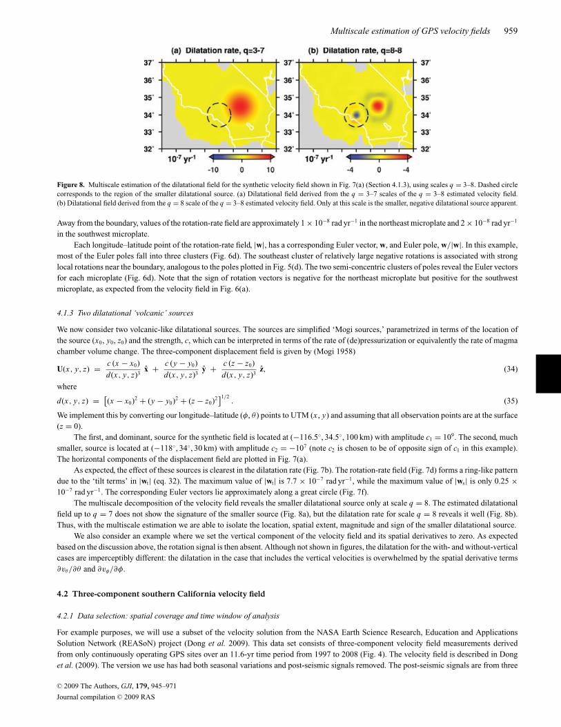
Figure 8. Multiscale estimation of the dilatational field for the synthetic velocity field shown in Fig. 7(a) (Section 4.1.3), using scales q = 3–8. Dashed circlecorresponds to the region of the smaller dilatational source. (a) Dilatational field derived from the q = 3–7 scales of the q = 3–8 estimated velocity field.(b) Dilatational field derived from the q = 8 scale of the q = 3–8 estimated velocity field. Only at this scale is the smaller, negative dilatational source apparent.

Away from the boundary, values of the rotation-rate field are approximately 1 × 10−8 rad yr−1 in the northeast microplate and 2 × 10−8 rad yr−1

in the southwest microplate.Each longitude–latitude point of the rotation-rate field, |w|, has a corresponding Euler vector, w, and Euler pole, w/|w|. In this example,

most of the Euler poles fall into three clusters (Fig. 6d). The southeast cluster of relatively large negative rotations is associated with stronglocal rotations near the boundary, analogous to the poles plotted in Fig. 5(d). The two semi-concentric clusters of poles reveal the Euler vectorsfor each microplate (Fig. 6d). Note that the sign of rotation vectors is negative for the northeast microplate but positive for the southwestmicroplate, as expected from the velocity field in Fig. 6(a).

4.1.3 Two dilatational ‘volcanic’ sources

We now consider two volcanic-like dilatational sources. The sources are simplified ‘Mogi sources,’ parametrized in terms of the location ofthe source (x0, y0, z0) and the strength, c, which can be interpreted in terms of the rate of (de)pressurization or equivalently the rate of magmachamber volume change. The three-component displacement field is given by (Mogi 1958)

U(x, y, z) = c (x − x0)

d(x, y, z)3x + c (y − y0)

d(x, y, z)3y + c (z − z0)

d(x, y, z)3z, (34)

where

d(x, y, z) = [(x − x0)2 + (y − y0)2 + (z − z0)2

]1/2. (35)

We implement this by converting our longitude–latitude (φ, θ ) points to UTM (x , y) and assuming that all observation points are at the surface(z = 0).

The first, and dominant, source for the synthetic field is located at (−116.5◦, 34.5◦, 100 km) with amplitude c1 = 109. The second, muchsmaller, source is located at (−118◦, 34◦, 30 km) with amplitude c2 = −107 (note c2 is chosen to be of opposite sign of c1 in this example).The horizontal components of the displacement field are plotted in Fig. 7(a).

As expected, the effect of these sources is clearest in the dilatation rate (Fig. 7b). The rotation-rate field (Fig. 7d) forms a ring-like patterndue to the ‘tilt terms’ in |wt| (eq. 32). The maximum value of |wt| is 7.7 × 10−7 rad yr−1, while the maximum value of |ws| is only 0.25 ×10−7 rad yr−1. The corresponding Euler vectors lie approximately along a great circle (Fig. 7f).

The multiscale decomposition of the velocity field reveals the smaller dilatational source only at scale q = 8. The estimated dilatationalfield up to q = 7 does not show the signature of the smaller source (Fig. 8a), but the dilatation rate for scale q = 8 reveals it well (Fig. 8b).Thus, with the multiscale estimation we are able to isolate the location, spatial extent, magnitude and sign of the smaller dilatational source.

We also consider an example where we set the vertical component of the velocity field and its spatial derivatives to zero. As expectedbased on the discussion above, the rotation signal is then absent. Although not shown in figures, the dilatation for the with- and without-verticalcases are imperceptibly different: the dilatation in the case that includes the vertical velocities is overwhelmed by the spatial derivative terms∂vθ/∂θ and ∂vφ/∂φ.

4.2 Three-component southern California velocity field

4.2.1 Data selection: spatial coverage and time window of analysis

For example purposes, we will use a subset of the velocity solution from the NASA Earth Science Research, Education and ApplicationsSolution Network (REASoN) project (Dong et al. 2009). This data set consists of three-component velocity field measurements derivedfrom only continuously operating GPS sites over an 11.6-yr time period from 1997 to 2008 (Fig. 4). The velocity field is described in Donget al. (2009). The version we use has had both seasonal variations and post-seismic signals removed. The post-seismic signals are from three

C© 2009 The Authors, GJI, 179, 945–971


960 C. Tape et al.

Figure 9. Base map for GPS velocity field study of southern California. Map shows topography and bathymetry (Amante & Eakins 2008), as well asactive faults (Jennings 1994), including the Kern Canyon fault (Nadin & Saleeby 2009). Labels 1–6 denote the sedimentary basins of Los Angeles (1),San Fernando (2), Ventura–Santa Barbara (3), Santa Maria (4), southern San Joaquin (5) and the Salton trough (6), all of which have been active duringthe Neogene. Faults labelled for reference are: San Andreas (SA), Kern Canyon (KC), Garlock (G), and Elsinore (E). Global CMT fault-plane solutions(Dziewonski & Woodhouse 1983) for large (Mw ≥ 6.0) earthquakes from 1990 to 2008 are: Landers (1992 June 28 Mw 7.3), Hector Mine (1999 October 16Mw 7.1), Northridge (1994 January 17 Mw 6.7), San Simeon (2003 December 22 Mw 6.6), Joshua Tree (1992 April 23 Mw 6.2), Eureka Valley (1993 May 17Mw 6.1) and Parkfield (2004 September 28 Mw 6.0). Inset map shows the plate boundary setting for western North America (Bird 2003).

earthquakes (Fig. 9): 1999 October 16 Mw 7.1 Hector Mine (e.g. Pollitz et al. 2001; Hudnut et al. 2002), 2003 December 22 Mw 6.5 SanSimeon (e.g. McLaren et al. 2008) and 2004 September 28 Mw 6.0 Parkfield (Savage & Langbein 2008).

A denser set of geodetic measurements for California can be found in the California Crustal Motion Map, version 1.0 (CCMM1; Shenet al. 2006), which was preceded by the SCEC Crustal Motion Map, v3.0 (Shen et al. 2003). (In the southern California region, CCMM1contains 1093 observations, while REASoN contains 408.) However, these data sets contain many campaign GPS sites, which are not asuseful for examining temporal variations, which is our ultimate objective.

In Fig. 4, we show our subset of the REASoN data set, including uncertainty estimates. The reference frame for the velocity field isITRF2005 (Altamimi et al. 2007), which leads to a significant component of rotation, when compared to a fixed-North-America referenceframe, for example. Thus, as described in Section 2.4, we estimate a single Euler vector for the field, and remove the least-squares best-fittingpurely rotational field (Figs 4a–c). The difference between the residual velocity field (c) and the original one (a) is a uniform rotation, whichhas no effect on quantities such as strain rate or dilatation rate.

4.2.2 Vertical velocity field

The vertical velocity field of our subset of the REASoN data set is plotted in Fig. 10(a). Since we are primarily interested in spatial gradients ofthe vertical field, we could remove a reference vertical rate to all points, similar to removing the effect of a uniform rotation on the horizontalfield. However, because the vertical velocities are distributed about 0 mm yr−1, we do not remove a reference value.

We estimate the vertical velocity field using scales q = 3–7 (Fig. 10b). In order to better fit the magnitude of the vertical field, we use aregularization parameter that is less than the minimum of the ordinary cross-validation function (Fig. 9). This underdamping leads to reducedresiduals in Fig. 10(c), but at the expense of more ‘oscillations’ from one scale to the next in the estimation (Figs 12g and j).

The estimated vertical field considers the uncertainty in the observations and helps reveal the primary features of the velocity field. Inparticular, observation points above the large sedimentary basins (San Joaquin, Ventura, Los Angeles, Salton) are going down, while regionsmoving up include Sierra Nevada (Fay et al. 2008), Parkfield, Transverse Ranges and the eastern Mojave. The residual field reveals a spatialpattern dominated by the strongest subsidence signals in the San Joaquin basin and the Salton trough (Fig. 10c ). By allowing for shorter

C© 2009 The Authors, GJI, 179, 945–971



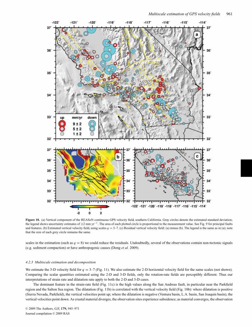
Figure 10. (a) Vertical component of the REASoN continuous GPS velocity field, southern California. Gray circles denote the estimated standard deviation;the legend shows uncertainty estimates of ±2 mm yr−1. The area of each plotted circle is proportional to the measurement value. See Fig. 9 for principal faultsand features. (b) Estimated vertical velocity field, using scales q = 3–7. (c) Residual vertical velocity field: (a) minus (b). The legend is the same as in (a); notethat the size of each grey circle remains the same.

scales in the estimation (such as q = 8) we could reduce the residuals. Undoubtedly, several of the observations contain non-tectonic signals(e.g. sediment compaction) or have anthropogenic causes (Dong et al. 2009).

4.2.3 Multiscale estimation and decomposition

We estimate the 3-D velocity field for q = 3–7 (Fig. 11). We also estimate the 2-D horizontal velocity field for the same scales (not shown).Comparing the scalar quantities estimated using the 2-D and 3-D fields, only the rotation-rate fields are perceptibly different. Thus ourinterpretations of strain rate and dilatation rate apply to both the 2-D and 3-D cases.

The dominant feature in the strain-rate field (Fig. 11c) is the high values along the San Andreas fault, in particular near the Parkfieldregion and the Salton Sea region. The dilatation (Fig. 11b) is correlated with the vertical velocity field (Fig. 10b): where dilatation is positive(Sierra Nevada, Parkfield), the vertical velocities point up; where the dilatation is negative (Ventura basin, L.A. basin, San Joaquin basin), thevertical velocities point down. As crustal material diverges, the observation sites experience subsidence; as material converges, the observation

C© 2009 The Authors, GJI, 179, 945–971


962 C. Tape et al.

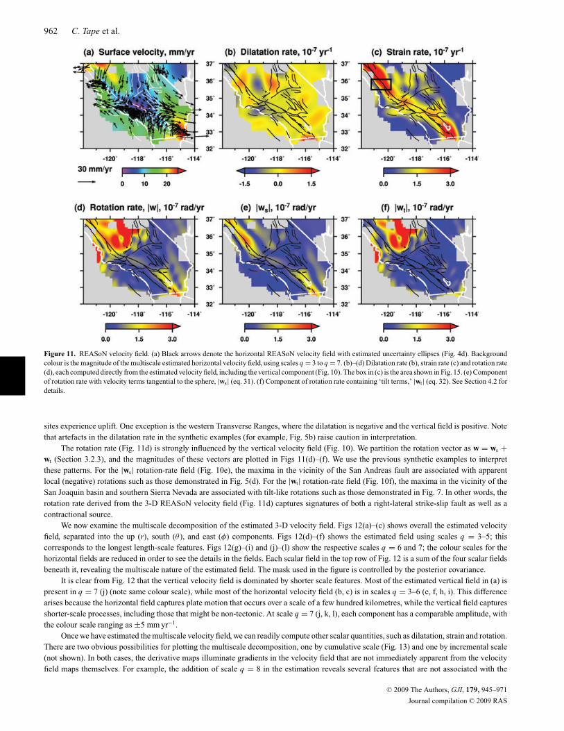
Figure 11. REASoN velocity field. (a) Black arrows denote the horizontal REASoN velocity field with estimated uncertainty ellipses (Fig. 4d). Backgroundcolour is the magnitude of the multiscale estimated horizontal velocity field, using scales q = 3 to q = 7. (b)–(d) Dilatation rate (b), strain rate (c) and rotation rate(d), each computed directly from the estimated velocity field, including the vertical component (Fig. 10). The box in (c) is the area shown in Fig. 15. (e) Componentof rotation rate with velocity terms tangential to the sphere, |ws| (eq. 31). (f) Component of rotation rate containing ‘tilt terms,’ |wt| (eq. 32). See Section 4.2 fordetails.

sites experience uplift. One exception is the western Transverse Ranges, where the dilatation is negative and the vertical field is positive. Notethat artefacts in the dilatation rate in the synthetic examples (for example, Fig. 5b) raise caution in interpretation.

The rotation rate (Fig. 11d) is strongly influenced by the vertical velocity field (Fig. 10). We partition the rotation vector as w = ws +wt (Section 3.2.3), and the magnitudes of these vectors are plotted in Figs 11(d)–(f). We use the previous synthetic examples to interpretthese patterns. For the |ws| rotation-rate field (Fig. 10e), the maxima in the vicinity of the San Andreas fault are associated with apparentlocal (negative) rotations such as those demonstrated in Fig. 5(d). For the |wt| rotation-rate field (Fig. 10f), the maxima in the vicinity of theSan Joaquin basin and southern Sierra Nevada are associated with tilt-like rotations such as those demonstrated in Fig. 7. In other words, therotation rate derived from the 3-D REASoN velocity field (Fig. 11d) captures signatures of both a right-lateral strike-slip fault as well as acontractional source.

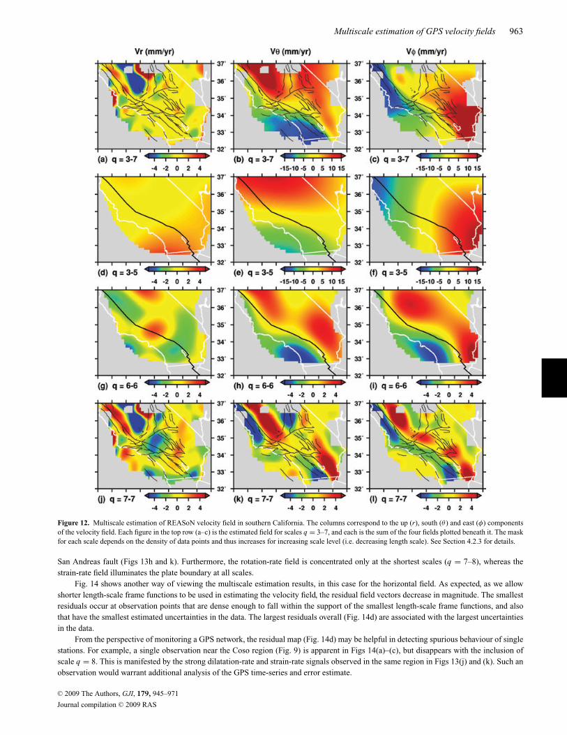
We now examine the multiscale decomposition of the estimated 3-D velocity field. Figs 12(a)–(c) shows overall the estimated velocityfield, separated into the up (r), south (θ ), and east (φ) components. Figs 12(d)–(f) shows the estimated field using scales q = 3–5; thiscorresponds to the longest length-scale features. Figs 12(g)–(i) and (j)–(l) show the respective scales q = 6 and 7; the colour scales for thehorizontal fields are reduced in order to see the details in the fields. Each scalar field in the top row of Fig. 12 is a sum of the four scalar fieldsbeneath it, revealing the multiscale nature of the estimated field. The mask used in the figure is controlled by the posterior covariance.

It is clear from Fig. 12 that the vertical velocity field is dominated by shorter scale features. Most of the estimated vertical field in (a) ispresent in q = 7 (j) (note same colour scale), while most of the horizontal velocity field (b, c) is in scales q = 3–6 (e, f, h, i). This differencearises because the horizontal field captures plate motion that occurs over a scale of a few hundred kilometres, while the vertical field capturesshorter-scale processes, including those that might be non-tectonic. At scale q = 7 (j, k, l), each component has a comparable amplitude, withthe colour scale ranging as ±5 mm yr−1.

Once we have estimated the multiscale velocity field, we can readily compute other scalar quantities, such as dilatation, strain and rotation.There are two obvious possibilities for plotting the multiscale decomposition, one by cumulative scale (Fig. 13) and one by incremental scale(not shown). In both cases, the derivative maps illuminate gradients in the velocity field that are not immediately apparent from the velocityfield maps themselves. For example, the addition of scale q = 8 in the estimation reveals several features that are not associated with the

C© 2009 The Authors, GJI, 179, 945–971



Figure 12. Multiscale estimation of REASoN velocity field in southern California. The columns correspond to the up (r), south (θ ) and east (φ) componentsof the velocity field. Each figure in the top row (a–c) is the estimated field for scales q = 3–7, and each is the sum of the four fields plotted beneath it. The maskfor each scale depends on the density of data points and thus increases for increasing scale level (i.e. decreasing length scale). See Section 4.2.3 for details.

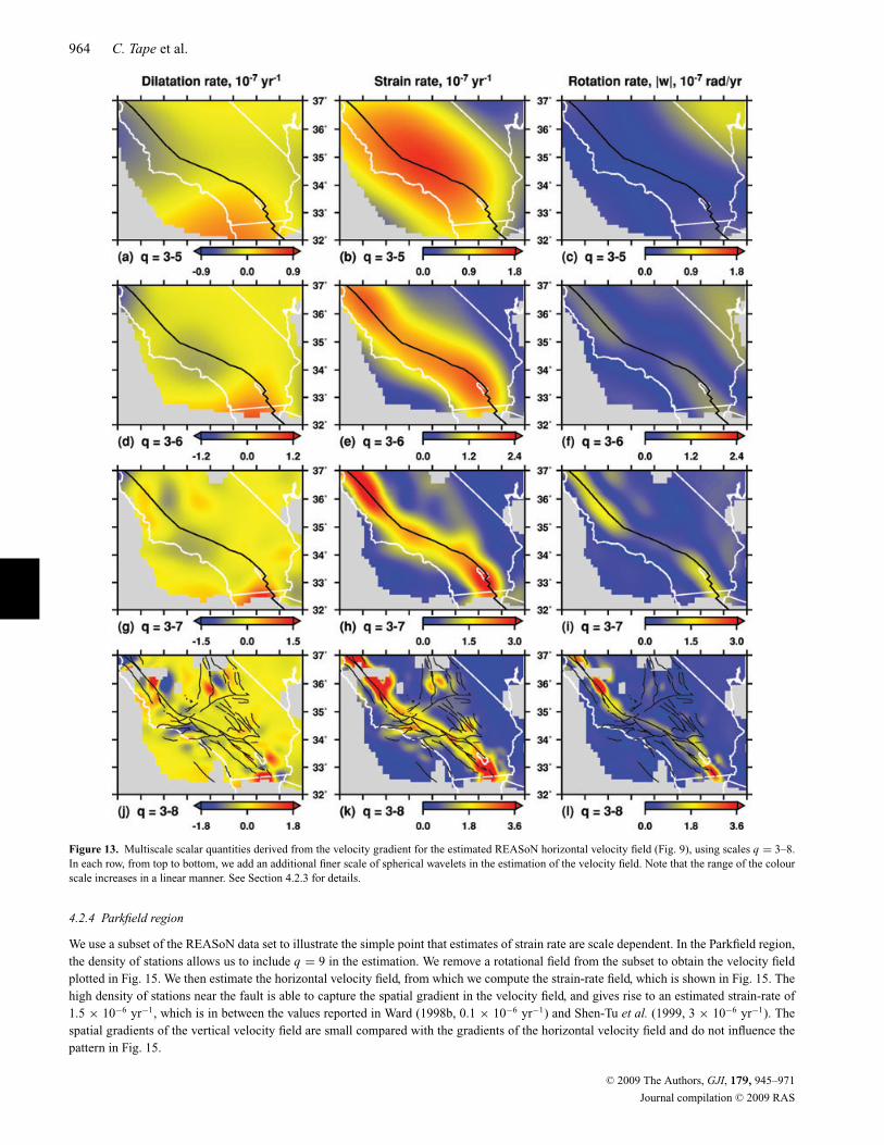
San Andreas fault (Figs 13h and k). Furthermore, the rotation-rate field is concentrated only at the shortest scales (q = 7–8), whereas thestrain-rate field illuminates the plate boundary at all scales.

Fig. 14 shows another way of viewing the multiscale estimation results, in this case for the horizontal field. As expected, as we allowshorter length-scale frame functions to be used in estimating the velocity field, the residual field vectors decrease in magnitude. The smallestresiduals occur at observation points that are dense enough to fall within the support of the smallest length-scale frame functions, and alsothat have the smallest estimated uncertainties in the data. The largest residuals overall (Fig. 14d) are associated with the largest uncertaintiesin the data.

From the perspective of monitoring a GPS network, the residual map (Fig. 14d) may be helpful in detecting spurious behaviour of singlestations. For example, a single observation near the Coso region (Fig. 9) is apparent in Figs 14(a)–(c), but disappears with the inclusion ofscale q = 8. This is manifested by the strong dilatation-rate and strain-rate signals observed in the same region in Figs 13(j) and (k). Such anobservation would warrant additional analysis of the GPS time-series and error estimate.

C© 2009 The Authors, GJI, 179, 945–971


964 C. Tape et al.

Figure 13. Multiscale scalar quantities derived from the velocity gradient for the estimated REASoN horizontal velocity field (Fig. 9), using scales q = 3–8.In each row, from top to bottom, we add an additional finer scale of spherical wavelets in the estimation of the velocity field. Note that the range of the colourscale increases in a linear manner. See Section 4.2.3 for details.

4.2.4 Parkfield region

We use a subset of the REASoN data set to illustrate the simple point that estimates of strain rate are scale dependent. In the Parkfield region,the density of stations allows us to include q = 9 in the estimation. We remove a rotational field from the subset to obtain the velocity fieldplotted in Fig. 15. We then estimate the horizontal velocity field, from which we compute the strain-rate field, which is shown in Fig. 15. Thehigh density of stations near the fault is able to capture the spatial gradient in the velocity field, and gives rise to an estimated strain-rate of1.5 × 10−6 yr−1, which is in between the values reported in Ward (1998b, 0.1 × 10−6 yr−1) and Shen-Tu et al. (1999, 3 × 10−6 yr−1). Thespatial gradients of the vertical velocity field are small compared with the gradients of the horizontal velocity field and do not influence thepattern in Fig. 15.

C© 2009 The Authors, GJI, 179, 945–971



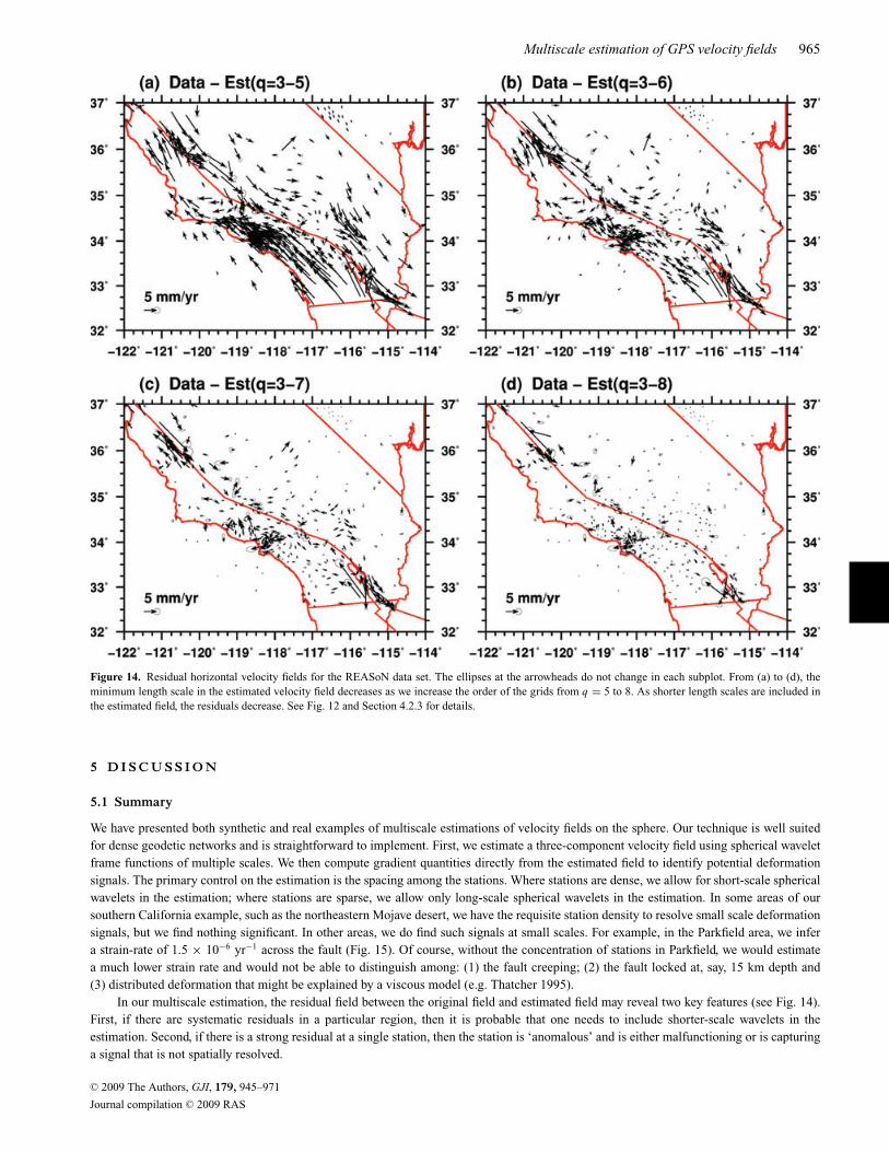
Figure 14. Residual horizontal velocity fields for the REASoN data set. The ellipses at the arrowheads do not change in each subplot. From (a) to (d), theminimum length scale in the estimated velocity field decreases as we increase the order of the grids from q = 5 to 8. As shorter length scales are included inthe estimated field, the residuals decrease. See Fig. 12 and Section 4.2.3 for details.

5 D I S C U S S I O N

5.1 Summary

We have presented both synthetic and real examples of multiscale estimations of velocity fields on the sphere. Our technique is well suitedfor dense geodetic networks and is straightforward to implement. First, we estimate a three-component velocity field using spherical waveletframe functions of multiple scales. We then compute gradient quantities directly from the estimated field to identify potential deformationsignals. The primary control on the estimation is the spacing among the stations. Where stations are dense, we allow for short-scale sphericalwavelets in the estimation; where stations are sparse, we allow only long-scale spherical wavelets in the estimation. In some areas of oursouthern California example, such as the northeastern Mojave desert, we have the requisite station density to resolve small scale deformationsignals, but we find nothing significant. In other areas, we do find such signals at small scales. For example, in the Parkfield area, we infera strain-rate of 1.5 × 10−6 yr−1 across the fault (Fig. 15). Of course, without the concentration of stations in Parkfield, we would estimatea much lower strain rate and would not be able to distinguish among: (1) the fault creeping; (2) the fault locked at, say, 15 km depth and(3) distributed deformation that might be explained by a viscous model (e.g. Thatcher 1995).

In our multiscale estimation, the residual field between the original field and estimated field may reveal two key features (see Fig. 14).First, if there are systematic residuals in a particular region, then it is probable that one needs to include shorter-scale wavelets in theestimation. Second, if there is a strong residual at a single station, then the station is ‘anomalous’ and is either malfunctioning or is capturinga signal that is not spatially resolved.

C© 2009 The Authors, GJI, 179, 945–971


966 C. Tape et al.

Figure 15. Strain-rate field derived from the multiscale estimation of the REASoN velocity field in the Parkfield region, using only scales q = 6–9. Theestimated strain rate across the San Andreas fault is about 1.5 × 10−6 yr−1. The superimposed velocity field observations, plotted as vectors, are obtained byfirst removing a uniform rotational field from the REASoN velocity field (e.g. Figs 4a–c). See Fig. 11(c) for context.

The synthetic examples (Section 4) illustrate several basic points. In the example with two dilatational sources, one much larger thanthe other, we saw the advantage of the separation of scales in identifying subtle signals. This example also suggests that derivative quantitiesbased on observations from multiple sites will perform better in detecting signals than the individual components of the velocity field andthat the vertical component, if available, should be used in estimating the velocity field, since deformation may not be predominantly in thehorizontal directions.

With the real observations (Section 4.2), we show the usefulness of separating the three-component velocity field into constituent scales.The vertical velocity field contains spatially coherent features with length scales typically less than those observed in the horizontal velocityfield, which reveal deformation across a broad plate boundary zone. The shortest length scales due to the horizontal deformation are foundin the regions of Parkfield and Salton Sea, as previously established (e.g. Ward 1998b). Although some of the vertical velocity observationsare certainly influenced by non-tectonic effects, they should still be included—along with proper uncertainty estimates—in the monitoring ofsignals in dense geodetic networks, especially in areas with larger expected vertical motions, such as subduction zones.

5.2 Regularization

Regularization is required to obtain a smooth estimated velocity field from the discrete observations. This is achieved through two possibleactions. First, one can cull the set of possible spherical wavelets based on the coverage of observations. If each spherical wavelet has a sufficientnumber of observations constraining its coefficient, then no regularization is needed (λ = 0). Second, if all spherical wavelets are used forthe inverse problem (eq. 15), then extensive regularization will be needed, since most wavelets will have zero observations constraining theircorresponding coefficients. In our approach, we have chosen something in between these two ‘end-members,’ where we at the outset eliminatemany candidate spherical wavelets based on data coverage (Fig. 3), but we still require a moderate amount of explicit regularization in theinversion (Fig. 2).

5.3 Towards multiscale time-dependent event detection

Our ultimate objective is to monitor time-dependent signals in dense GPS networks. Because our emphasis is on continuously recording GPSnetworks, our station coverage is not as dense as many published velocity fields, which include campaign GPS measurements (e.g. Shen et al.2006; McCaffrey et al. 2007). In this study, we have only dealt with the spatial part of the problem, showing that the multiscale representationis well suited to identifying and characterizing geophysical signals of all scales. It also has the potential capability of removing scale-specificnoise. This approach is a step towards global multiscale monitoring of time-dependent GPS displacement fields, in hopes of efficient andaccurate characterization of Earth’s surface deformation and the detection of geophysically important phenomena.

A C K N OW L E D G M E N T S

We are grateful to John Haines, an anonymous reviewer, and editor John Beavan for comments that improved this manuscript. We thankJean-Philippe Avouac for helpful discussions. We acknowledge the Southern California Integrated GPS Network and its sponsors, the W.M.Keck Foundation, NASA, NSF, USGS and SCEC, for providing data used in this study. This research was supported in part by the Gordonand Betty Moore Foundation. This is Caltech Tectonic Observatory Contribution 112.

C© 2009 The Authors, GJI, 179, 945–971



R E F E R E N C E S

Allmendinger, R.W., Reilinger, R. & Loveless, J., 2007. Strain and rota-tion rate from GPS in Tibet, Anatolia, and the Altiplano, Tectonics, 26,TC3013, doi:10.1029/2006TC002030.

Altamimi, Z., Collilieux, X., Legrand, J., Garayt, B. & Boucher, C., 2007.ITRF2005: A new release of the International Terrestrial Reference Framebased on time series of station positions and Earth Orientation Parameters,J. geophys. Res., 112, B09401, doi:10.1029/2007JB004949.

Amante, C. & Eakins, B.W., 2008. ETOPO1 1 Arc-Minute Global ReliefModel: Procedures, Data Sources and Analysis, National GeophysicalData Center, NESDIS, NOAA, U.S. Department of Commerce, Boulder,CO, USA.

Antoine, J.P. & Vandergheynst, P., 1999. Wavelets on the 2-sphere:a group-theoretical approach, Appl. Comput. Harmonic Anal., 7(3),262–291.

Argus, D.F., Heflin, M.B., Peltzer, G., Crampe, F. & Webb, F.H., 2005. In-terseismic strain accumulation and anthropogenic motion in metropolitanLos Angeles, J. geophys. Res., 110, B04401, doi:10.1029/2003JB002934.

Bayer, M., Freeden, W. & Maier, T., 2001. A vector wavelet approach toiono- and magnetospheric geomagnetic satellite data, J. Atmos. Solar-Terr.Phys., 63, 581–597.

Beavan, J. & Haines, J., 2001. Contemporary horizontal veloc-ity and strain rate fields of the Pacific-Australian plate bound-ary zone through New Zealand, J. geophys. Res., 106(B1), 741–770.

Becker, T.W., Hardebeck, J.L. & Anderson, G., 2005. Constraints on faultslip rates of the southern California plate boundary from GPS velocityand stress inversions, Geophys. J. Int., 160, 634–650.

Bird, P., 2003. An updated digital model of plate boundaries, Geochem.Geophys. Geosyst., 4, 1–52.

Bogdanova, I., Vandergheynst, P., Antoine, J.R., Jacques, L. & Morvidone,M., 2005. Stereographic wavelet frames on the sphere, Appl. Comput.Harmonic Anal., 19(2), 223–252.

Bos, A.G., Spakman, W. & Nyst, M.C.J., 2003. Surface deformation andtectonic setting of Taiwan inferred from a GPS velocity field, J. geophys.Res., 108(B10), 2458, doi:10.1029/2002JB002336.

Chambodut, A., Panet, I., Mandea, M., Diament, M., Holschneider, M. &Jamet, O., 2005. Wavelet frames: an alternative to spherical harmonicrepresentation of potential fields, Geophys. J. Int., 163(3), 875–899.

Chinnery, M.A., 1961. The deformation of the ground around surface faults,Bull. seism. Soc. Am., 51(3), 355–372.

Dahlke, S. & Maass, P., 1996. Continuous wavelet transforms with appli-cations to analyzing functions on spheres, J. Fourier Anal. Appl., 2(4),379–396.

Dong, D., Fang, P., Bock, Y., Prawirodirdjo, L., Webb, F., Kedar, S. & Lund-gren, P., 2009. Secular vertical crustal deformation field in Californiaand Nevada regions from GPS data analysis: 1. Hydrological and anthro-pogenic signals, J. geophys. Res, in preparation.

Dragert, H., Wang, K. & James, T.S., 2001. A silent slip event on the deeperCascadia subduction interface, Science, 292, 1525–1528.

Dziewonski, A. & Woodhouse, J.H., 1983. Studies of the seismic sourceusing normal-mode theory, in Earthquakes: Observation, Theory andInterpretation: Notes from the International School of Physics ‘EnricoFermi’ (1982, Varenna, Italy), Vol. LXXXV, pp. 45–137, eds Kanamori,H. & Boschi, E., North-Holland Pub., Amsterdam.

Fay, N.P., Bennett, R.A. & Hreinsdottir, S., 2008. Contemporary verticalvelocity of the central Basin and Range and uplift of the southern SierraNevada, Geophys. Res. Lett., 35, L20309, doi:10.1029/2008GL034949.

Feigl, K.L., King, R.W. & Jordan, T.H., 1990. Geodetic measurement oftectonic deformation in the Santa Maria fold and thrust belt, California,J. geophys. Res., 95(B3), 2679–2699.

Flesch, L.M., Holt, W.E., Silver, P.G., Stephenson, M., Wang, C.-Y. & Chan,W.W., 2005. Constraining the extent of crust–mantle coupling in centralAsia using GPS, geologic, and shear wave splitting data, Earth planet.Sci. Lett., 238, 248–268.

Freeden, W. & Windheuser, U., 1996. Spherical wavelet transform and itsdiscretization, Adv. Comput. Math., 5(1), 51–94.

Freeden, W. & Windheuser, U., 1997. Combined spherical harmonic andwavelet expansion—a future concept in earth’s gravitational potential de-termination, Appl. Comput. Harmonic Anal., 4, 1–37.

Golub, G.H. & Van Loan, C.F., 1989. Matrix Computations, 2nd edn, JohnsHopkins Univ. Press, Baltimore, MD, USA.

Golub, G.H., Heath, M. & Wahba, G., 1979. Generalized cross-validationas a method for choosing a good ridge parameter, Technometrics, 21,215–223.

Guilloux, F., Fay, G. & Cardoso, J.-F., 2009. Practical wavelet design on thesphere, Appl. Comput. Harmonic Anal., 26(2), 143–160.

Haines, A.J. & Holt, W.E., 1993. A procedure for obtaining the completehorizontal motions within zones of distributed deformation from the in-version of strain rate data, J. geophys. Res., 98(B7), 12 057–12 082.

Hastie, T. & Loader, C., 1993. Local regression: automatic kernel carpentry,Stat. Sci., 8(2), 120–143.

Heki, K., 1997. Silent fault slip following an interplate thrust earthquake atthe Japan Trench, Nature, 386, 595–598.

Holschneider, M., 1996. Continuous wavelet transforms on the sphere,J. Math. Phys., 37(8), 4156–4165.

Holschneider, M., Chambodut, A. & Mandea, M., 2003. From global to re-gional analysis of the magnetic field on the sphere using wavelet frames,Phys. Earth planet. Inter., 135, 107–124.

Holt, W.E., Chamot-Rooke, N., Pichon, X.L., Haines, A.J., Shen-Yu, B.& Ren, J., 2000. Velocity field in Asia inferred from Quaternary faultslip rates and Global Positioning System observations, J. geophys. Res.,105(B8), 19 185–19 209.

Hsu, Y.-J., Yu, S.-B., Simons, M., Kuo, L.-C. & Chen, H.-Y., 2009. Interseis-mic crustal deformation in the Taiwan plate boundary zone revealed byGPS observations, seismicity, and earthquake focal mechanisms, Tectono-physics, in press.

Hudnut, K.W. et al., 2002. Continuous GPS observations of postseismicdeformation following the 16 October 1999 Hector Mine, California,earthquake (Mw 7.1), Bull. seism. Soc. Am., 92(4), 1403–1422.

Jennings, C.W., 1994. Fault activity map of California and adjacent areas,with locations and ages of recent volcanic eruptions, Calif. Div. Minesand Geology, Geologic Data Map No. 6, map scale 1:750,000.

Kovacevic, J. & Chebira, A., 2007a. Life beyond bases: the advent of frames(Part I), IEEE Signal Process. Mag., 24(4), 86–104.

Kovacevic, J. & Chebira, A., 2007b. Life beyond bases: the advent of frames(Part II), IEEE Signal Process. Mag., 24(5), 115–125.

Kreemer, C., Holt, W.E. & Haines, A.J., 2003. An integrated global modelof present-day plate motions and plate boundary deformation, Geophys.J. Int., 154, 8–34.

Malvern, L.E., 1969. Introduction to the Mechanics of a ContinuousMedium, Prentice-Hall, Upper Saddle River, NJ, USA.

Matheron, G., 1963. Principles of geostatistics, Econ. Geol., 58, 146–1266.McCaffrey, R. et al., 2007. Fault locking, block rotation and crustal defor-

mation in the Pacific Northwest, Geophys. J. Int., 169, 1315–1340.McGuire, J.J. & Segall, P., 2003. Imaging of aseismic fault slip transients

recorded by dense geodetic networks, Geophys. J. Int., 155, 778–788.McLaren, M.K., Hardebeck, J.L., van der Elst, N., Unruh, J., Bawden, G.W.

& Blai, J.L., 2008. Complex faulting associated with the 22 Decem-ber 2003 MW 6.5 San Simeon, California, earthquake, aftershocks, andpostseismic surface deformation, Bull. seism. Soc. Am., 98(4), 1659–1680.

Meade, B.J. & Hager, B.H., 2005. Block models of crustal motion in south-ern California constrained by GPS measurements, J. geophys. Res., 110,B03403, doi:10.1029/2004JB003209.

Meade, B.J., Hager, B.H., McClusky, S.C., Reilinger, R.E., Ergintav, S.,Lenk, O., Barka, A. & Ozener, H., 2002. Estimates of seismic potential inthe Marmara Sea region from block models of secular deformation con-strained by Global Positioning System measurements, Bull. seism. Soc.Am., 92, 208–215.

Melbourne, T.I., Webb, F.H., Stock, J.M. & Reigber, C., 2002. Rapid post-seismic transients in subduction zones from continuous GPS, J. geophys.Res., 107(B10), 2241, doi:10.1029/2001JB000555.

Menke, W., 1989. Geophysical Data Analysis: Discrete Inverse Theory,Academic Press, San Diego, CA, USA.

C© 2009 The Authors, GJI, 179, 945–971


968 C. Tape et al.

Miyazaki, S., McGuire, J.J. & Segall, P., 2003. A transient subduction zoneslip episode in southwest Japan observed by the nationwide GPS array, J.geophys. Res., 108(B2), 2087, doi:10.1029/2001JB000456.

Miyazaki, S., Segall, P., Fukuda, J. & Kato, T., 2004. Space time distribu-tion of afterslip following the 2003 Tokachi-oki earthquake: Implicationsfor variations in fault zone frictional properties, Geophys. Res. Lett., 31,L06623, doi:10.1029/2003GL019410.

Mogi, K., 1958. Relations between the eruptions of various volcanoes andthe deformations of the ground surfaces around them, Bull. Earthq. Res.Inst., 36, 99–134.

Nadin, E.S. & Saleeby, J.B., 2009. Quaternary reactivation of the KernCanyon fault system, southern Sierra Nevada, California, USA, Geol.Soc. Am. Bull., in press.

Oh, H.-S. & Li, T.-H., 2004. Estimation of global temperature fields fromscattered observations by a spherical-wavelet-based spatially adaptivemethod, J. R. Statist. Soc. B, 66, 221–238.

Ozawa, S., Murakami, M., Kaidzu, M., Tada, T., Sagiya, T., Hatanaka, Y.,Yarai, H. & Nishimura, T., 2002. Detection and monitoring of the ongo-ing aseismic slip in the Tokai region, Central Japan, Science, 298, 1009–1012.

Pollitz, F.F., Wicks, C. & Thatcher, W., 2001. Mantle flow beneath a con-tinental strike-slip fault: Postseismic deformation after the 1999 HectorMine earthquake, Science, 293, 1814–1818.

Pritchard, M.E. & Simons, M., 2006. An aseismic slip pulse in northernChile and along-strike variations in seismogenic behavior, J. geophys.Res., 111, B08405, doi:10.1029/2006JB0042580.

Reguzzoni, M., Sanso, F. & Venuti, G., 2005. The theory of general kriging,with applications to the determination of a local geoid, Geophys. J. Int.,162, 303–314.

Rogers, G. & Dragert, H., 2003. Episodic tremor and slip on the Cas-cadia subduction zone: The chatter of silent slip, Science, 300, 1942–1943.

Savage, J.C. & Langbein, J., 2008. Postearthquake relaxation after the 2004M6 Parkfield, California, earthquake and rate-and-state friction, J. geo-phys. Res., 113, B10407, doi:10.1029/2008JB005723.

Savage, J.C. & Prescott, W.H., 1976. Strain accumulation on the San Jac-into fault near Riverside, California, Bull. seism. Soc. Am., 66(5), 1749–1754.

Shao, J., 1993. Linear model selection by cross-validation, J. Am. Stat. As-soc., 88, 486–494.

Shao, J., 1997. An asymptotic theory for linear model selection, Stat. Sin.,7, 221–242.

Shearer, P.M., 1999. Introduction to Seismology, Cambridge Univ. Press,Cambridge, UK.

Shen, Z.-K., Jackson, D.D. & Ge, B.X., 1996. Crustal deformation across and

beyond the Los Angeles basin from geodetic measurements, J. geophys.Res., 101(B12), 27 957–27 980.

Shen, Z.-K. et al., 2003. The SCEC Crustal Motion Map, version 3.0, avail-able online at http://epicenter.usc.edu/cmm3/.

Shen, Z.-K., King, R.W., Agnew, D.C. & Wang, M., 2006. The Califor-nia Crustal Motion Map, version 1.0, in SCEC 2006 Annual MeetingAbstracts, Palm Springs, Calif. (Sept. 11–13, 2006).

Shen-Tu, B., Holt, W.E. & Haines, A.J., 1999. Deformation kinematics inthe western United States determined from Quaternary fault slip rates andrecent geodetic data, J. geophys. Res., 104(B12), 28 927–28 955.

Silverman, B.W., 1986. Density Estimation for Statistics and Data Analysis,Vol. 26 of Monographs on Statistics and Applied Probability, Chapmanand Hall, New York.

Simons, F.J., Dahlen, F.A. & Wieczorek, M.A., 2006. Spatiospectral con-centration on a sphere, SIAM Rev., 48(3), 504–536.

Simons, M. & Hager, B.H., 1997. Localization of the gravity field and thesignature of glacial rebound, Nature, 390, 500–504.

Simons, M., Solomon, S.C. & Hager, B.H., 1997. Localization of gravity andtopography: constraints on the tectonics and mantle dynamics of Venus,Geophys. J. Int., 131, 24–44.

Spakman, W. & Nyst, M.C.J., 2002. Inversion of relative motion data forestimates of the velocity gradient field and fault slip, Earth planet. Sci.Lett., 203, 577–591.

Tarantola, A., 2005. Inverse Problem Theory and Methods for Model Pa-rameter Estimation, SIAM, Philadelphia, PA, USA.

Teza, G., Pesci, A. & Galgaro, A., 2008. Grid strain and grid strain3: soft-ware packages for strain field computation in 2D and 3D environments,Comput. Geosci., 34(9), 1142–1153.

Thatcher, W., 1995. Microplate versus continuum description of active tec-tonic deformation, J. geophys. Res., 100(B3), 3885–3894.

Wahba, G., 1981. Spline interpolation and smoothing on the sphere, SIAMJ. Sci. Stat. Comp., 2(1), 5–16.

Walcott, R.I., 1973. Structure of the earth from glacio-isostatic rebound,Annu. Rev. Earth planet. Sci., 1, 15–37.

Wang, Z. & Dahlen, F.A., 1995. Spherical-spline parameterization of three-dimensional Earth, Geophys. Res. Lett., 22, 3099–3102.

Ward, S.N., 1998a. On the consistency of earthquake moment release andspace geodetic strain rates: Europe, Geophys. J. Int., 135, 1011–1018.

Ward, S.N., 1998b. On the consistency of earthquake moment rates, geo-logical fault data, and space geodetic strain: the United States, Geophys.J. Int., 134, 172–186.

Weisberg, S., 2005. Applied Linear Regression, 5th edn, Wiley, Hoboken,NJ, USA.

Wiaux, Y., Jacques, L. & Vandergheynst, P., 2005. Correspondence principlebetween spherical and Euclidean wavelets, Astrophys. J., 632(1), 15–28.

A P P E N D I X A : C O N S T RU C T I O N O F A F R A M E O F D O G S P H E R I C A L WAV E L E T S

The ‘Difference of Gaussians’ (DOG) spherical wavelet, of scale a, centred at pole x ∈ S2, defined by Bogdanova et al. (2005) is given by thefollowing expression

ψx,a(x′) = λa(γ )1/2 exp

[− tan2(γ /2)

a2

]− 1

αλαa(γ )1/2 exp

[− tan2(γ /2)

(αa)2

], (A1)

where α > 1 is a fixed number, γ is the angle between poles x and x′ and the parametric function λ is given by

λa(γ ) = 4a2

[(a2 − 1) cos γ + (a2 + 1)]2. (A2)

A DOG spherical wavelet ψz,a with parameter α = 1.25, centred at the North Pole z, is plotted in Fig. 1(b), for three different scales.Fig. 1(c) shows the corresponding profiles, for a fixed longitude φ. Fig. 1(d) displays their spectra (i.e. the spherical harmonics coefficientsl �→ |�z,a(l, 0)|, where �z,a(l, m) = ∫S2 ψz,aYl,md).

A frame of DOG spherical wavelets can be obtained by appropriate discretization of position x and scale a. Let Gq denote a grid ofvertices on the sphere, at a scale q. We are interested in defining a set of grids {Gq , q = 0, 1, . . .} having the following properties.

(i) The geodesic distance between neighbouring vertices is nearly uniform. This provides nearly uniform coverage for a given scale.(ii) Gq ⊂ Gq+1: vertices in the grid at scale q are also vertices in grids at finer scales. This is a requirement for multiscale analysis.

C© 2009 The Authors, GJI, 179, 945–971



A grid generated by successive subdivisions of an initial icosahedron satisfies these properties. Given an initial icosahedron G0, each triangleis subdivided into four new equilateral triangles, and the new vertices are projected into the sphere. As examples, we show meshes G2,G3

and G4 in Fig. 1(a). The geometric properties of the spherical-triangular grids are summarized in Table 2. For each scale q, the average sidearc-length Lq measures the sampling density on the sphere; the average sampling frequency is then given by 2π/Lq . Assuming that thissampling is uniform (the approximation is reasonable for our meshes), for a spherical function f ∈ L(S2) to be well sampled by the grid Gq ,it follows from Nyquist criterion that its bandwidth cannot exceed the value π/Lq . The maximum bandwidth lq = int(π/Lq ) associated toeach grid scale level q is shown in the rightmost column of Table 2.

The frame of spherical wavelets will be defined as the set F = {ψx(q, j),aq (x), x(q, j) ∈ Gq , q ∈ N}. The set is built by considering, for eachgrid Gq , all the wavelets with scale aq centred at its gridpoints. The choice of the scale aq associated to each grid resolution q is not arbitrary.Let BQ denote the set of functions of bandwidth B ≤ BQ . We want to define the set FQ = {ψx(q, j),aq (x), x(q, j) ∈ Gq , q = 0, . . . , Q} in sucha way that Span(FQ) = BQ . This requirement can only be satisfied if the union of the spectral support of all wavelets with scale aq , q ≤ Q,lies in the interval [0, BQ]. Since we want this condition to be true for all Q ≥ 1, it follows that the spectral support of the wavelets with scaleaq has to be the interval [bQ , BQ], for some bQ ≤ BQ−1. In other words, scale should be discretized in such a way that the family ofwavelets in the set F covers the spectrum, and the cardinal of F is not too large. Alternatively, if we view the wavelets as interpolatingfunctions, the wavelet scale aq associated to the grid Gq cannot oscillate more than what is permitted by the grid resolution samplingfrequency lq .

In the case of DOG spherical wavelets, the spectral support is not compact, but most of the energy (at least 99.0 per cent) is concentratedin a relatively small number of spherical harmonic coefficients, corresponding to the lowest spherical harmonics degrees (see Fig. 1d). Table 3shows, for DOG wavelets with scales aq = 2−q , q = 0, . . . , 10, the spherical harmonic degrees at which the energy reaches 99.0 per centand 99.9 per cent of the total energy. By comparing these values with the value lq in the rightmost column in Table 2, one can see thatthe choice aq = 2−q is well adapted to the grid resolution. Fig. 1(d) also illustrates the good spectral coverage obtained with this scalediscretization.

A P P E N D I X B : S E L E C T I O N O F T H E R E G U L A R I Z AT I O N PA R A M E T E R

The least-squares solution via Tikhonov regularization to the overdetermined problem is given by

m′ = (G′T G′ + λ2I)−1

G′T d′. (B1)

We review that (B1) is a general form of (13). Using the substitutions

m′ = S1/2 m, (B2)

G′ = Z1/2 G S−1/2, (B3)

d′ = Z1/2 d, (B4)

where S and Z are symmetric, square-root invertible matrices, we transform (B1) into (13)

S1/2 m = [(Z1/2 G S−1/2)T (Z1/2 G S−1/2) + λ2I]−1(Z1/2 G S−1/2)T Z1/2 d (B5)

m = S−1/2[S−1/2 GT Z GT S−1/2 + λ2I]−1S−1/2 GT Z d (B6)

= [S1/2(S−1/2 GT Z GT S−1/2 + λ2I)S1/2]−1GT Z d (B7)

= (GT Z GT + λ2 S)−1GT Z d. (B8)

Making the substitution Z = C−1D , we obtain (13). Thus, the inclusion of the weighting matrix for observations and the regularization matrix

for the model parameters is equivalent to the solution in (B1) with the transformations in (B2)–(B4). In other words, the selection of λ maybe discussed in the context of (B1) rather than (13).

Our choice of the regularization parameter is based on cross-validation (Golub et al. 1979; Shao 1993, 1997), which assume Gaussianuncertainties of the observations, and is based upon the fact that a good regularization parameter should provide good estimates for withhelddata. We used ‘ordinary cross-validation’, also known as ‘leave-one-out cross-validation’ or ‘delete-1 cross-validation.’ This involvesremoving one observation, computing a model vector, and then computing the cross-validated residual, which is the residual between thevalue at the removed point and the estimated value at the removed point. It turns out that n separate regressions are not needed to computethe cross-validation prediction error (e.g. Weisberg 2005, p. 291-292). The ith cross-validation residual can be written as

e(i) ≡ di − d(i) = di − di

1 − Nii (λ), (B9)

where

N(λ) = G(GT G + λ2I)−1GT (B10)

C© 2009 The Authors, GJI, 179, 945–971


970 C. Tape et al.

is the regularized data resolution matrix for the overdetermined least-squares problem (e.g. Menke 1989), λ is the regularization parameter,di is the estimated value from a model obtained by using all n observations, and d(i) is the estimated value from a model obtained by usingn − 1 observations.

The ordinary cross-validation function is defined in terms of eq. (B9) as

H (λ) = 1

n

n∑i=1

e2(i) = 1

n

n∑i=1

[di − di

1 − Nii (λ)

]2

. (B11)

For our examples, the curve H (λ) provided a single minimum from which we selected the regularization parameter. Fig. 2 shows log 10 H (λ)for three components of the velocity field.

A P P E N D I X C : D E F O R M AT I O N G R A D I E N T F O R E L A S T I C R H E O L O G Y

Here we show the steps used to derive eqs (20) and (21). For an isotropic linear elastic solid, the stress tensor σ = c : ε reduces to (e.g. Shearer1999, eq. 2.24)

σ =

⎡⎢⎢⎣λ Tr(ε) + 2με11 2με12 2με13

σ12 λ Tr(ε) + 2με22 2με23

σ13 σ23 λ Tr(ε) + 2με33

⎤⎥⎥⎦ . (C1)

Combining the constraints in eq. (19) with eq. (C1), and solving for the strain components, we obtain

ε11 = F (ε22 + ε33) , ε12 = 0, ε13 = 0. (C2)

where F is a constant (eq. 22). Hence, the strain tensor for an isotropic solid is given by

ε0 =

⎡⎢⎣ F (ε22 + ε33) 0 00 ε22 ε23

0 ε23 ε33

⎤⎥⎦ , (C3)

where the 0-subscript denotes that it is evaluated at the surface.Considering a time increment, �t , we have ε → D. With these assumptions, for an observation point at the surface (r = R), eq. (16)

reduces to eq. (20), where we used the constraints

∂vr

∂r= F

[1

R

(vr + ∂vθ

∂θ

)+ 1

R


sin θ

∂vφ

∂φ

)],

1

2R

(−vθ + ∂vr

∂θ+ R

∂vθ

∂r

)= 0,

1

2R

(−vφ + 1

sin θ

∂vr

∂φ+ R

∂vφ

∂r

)= 0,

which can be solved for the radial gradients (at r = R) to obtain

∂vr

∂r= F

R

(2vr + vθ cot θ + ∂vθ

∂θ+ 1

sin θ

∂vφ

∂φ

), (C4)

∂vθ

∂r= 1

R

(vθ − ∂vr

∂θ

), (C5)

∂vφ

∂r= 1

R

(vφ − 1

sin θ

∂vr

∂φ

). (C6)

Substituting these equations into eq. (17), the rotation-rate tensor (at r = R) reduces to eq. (21).

A P P E N D I X D : M AT R I X N O R M

We denote the N × N tensor T in its eigenbasis as

T = V�V−1, (D1)

where V contains the eigenvectors of T, and � is a diagonal matrix of corresponding eigenvalues λk . Using the property Tr(AB) = Tr (BA)with eq. (D1), one can obtain

Tr(Tp) =N∑

k=1

λpk . (D2)

C© 2009 The Authors, GJI, 179, 945–971



Because the eigenvalues of tensor T are invariant to coordinate changes, the operation Tr (Tp) is also invariant for any p.A common matrix norm is the Frobenius norm, defined as (Golub & Van Loan 1989, p. 56)

‖T‖F =⎛⎝ N∑

i=1

N∑j=1

|Ti j |2⎞⎠1/2

. (D3)

If T is real-valued, then

‖T‖2F = T : T, (D4)

where the ‘:’ denotes the scalar product of two tensors (Malvern 1969, p. 35)

T : T =N∑

i=1

N∑j=1

Ti j Ti j . (D5)

If T is symmetric, then

‖T‖2F = T : T = tr (TT) =

N∑k=1

λ2k . (D6)

C© 2009 The Authors, GJI, 179, 945–971


multiscale estimation of gps velocity ﬁelds · multiscale estimation of gps velocity ﬁelds 947...

Documents