THE MARKET REACTION TO STOCK SPLIT

ON ACTUAL STOCK SPLIT DAY

by Yu Huang

Bachelor of Business Administration, Beijing Normal University–

Hong Kong Baptist University United International College, 2013

and

Yixin Fan

Bachelor of Business Administration, Hunan University, 2012

PROJECT SUBMITTED IN PARTIAL FULFILLMENT OF THE REQUIREMENTS FOR THE DEGREE OF

MASTER OF SCIENCE IN FINANCE

In the Master of Science in Finance Program

of the

Faculty

of

Business Administration

Yu Huang and Yixin Fan 2014

SIMON FRASER UNIVERSITY

Fall 2014

 

Approval

Name: Yu Huang and Yixin Fan

Degree: Master of Science in Finance

Title: The Market Reaction to Stock Split on actual stock split day

Supervisory Committee:

________________________________

Alexander Vedrashko

Senior Supervisor

Associate Professor, Faculty of Business Administration

________________________________

Amir Rubin

Second Reader

Associate Professor, Faculty of Business Administration

Date Approved: ________________________________

 

 

 

 

 

 

 

 

Abstract

It is well documented in the literature that there are positive abnormal returns on the announcement days of stock splits. However, few studies investigated the stock return on the actual split day. We examine market reaction on the actual split day and find that it is positive. We also find a negative relationship between the market reaction and firm size as well as the previous trading volume. The result is in support of the inattention theory.

Key words: Stock Splits; Actual split day; Inattention Theory;

 

Acknowledgements

First and for most, we would like to express our sincerest gratitude to our supervisor, Dr. Alexander Vedrashko, who supported us throughout our thesis with his patience and rich empirical research knowledge. He always inspires us with new idea and guides us to reach the goal. Meanwhile, he allows us to go through the process of writing and analyzing thesis gently, gives us room to work in our own way. Every time we meet, we are encouraged and affected by his humors and volubility. Second, we would like to give our special thanks to our second reader, Amir Rubin, for the support to our final project. Finally, the Segal Graduate School of Business also provides the necessary support and equipment we need to complete the thesis.

 

 

 

 

 

 

 

 

 

 

 

 

 

 

 

 

Table of Content

Approval ........................................................................................................................ 0

Abstract .......................................................................................................................... 0

Acknowledgements ........................................................................................................ 0

1 Introduction ................................................................................................................. 1

2 Literature review ......................................................................................................... 3 2.1 Positive Signal Hypothesis .............................................................................................. 4

2.2 Optimal Trading Range Hypothesis ................................................................................. 4

2.3 The Neglected-Firm Hypothesis ...................................................................................... 5

2.4 Liquidity Hypothesis ....................................................................................................... 6

2.5 The dividend hypothesis .................................................................................................. 6

3 Data Analysis .............................................................................................................. 7 3.1 Data Description .............................................................................................................. 7

3.2 Summary statistics and T-test for abnormal return .......................................................... 8

3.3 Test for the influence from

firm size, price before split,split size and volume ........................................................... 8

3.4 Regression ...................................................................................................................... 11

4 Conclusion…………………….………………………………….…..…………… 13

References .................................................................................................................... 14 Appendix……………………………………………………………………………..16  

 

 

 

 

 

 

 

List of Tables

Table 1: Summary statistics and t-test results for the BHAR in each period ............... 16 Table 2: Summary statistics and t-test results for the BHAR:

large vs small firms ....................................................................................... 17 Table 3: Summary statistics and t-test results for the BHAR:

Price quartiles ................................................................................................ 18 Table 4: Summary statistics and t-test results for the BHAR:

Split size ........................................................................................................ 19 Table 5: Summary statistics and t-test results for the monthly volume:

Before and after ............................................................................................. 20 Table 6: Summary statistics and t-test results for the BHAR:

High vs low monthly volume before split ..................................................... 21 Table 7: Regression Results ......................................................................................... 22

 

 

 

1 

1 Introduction

Do stock splits affect stock prices and returns? This question was extensively

discussed and researched among scholars over the past decades. Countless studies

have been carried out and many empirical tests have proved that the announcement of

stock splits do affect the stock price and bring abnormal return on and after the stock

split announcement day. For instance, Li, Stork, and Zou (2013) analyzed the market

reaction to stock splits announcements using a unique US sample over the period

2000 to 2009 and found a significantly positive Cumulative Average Abnormal Return

(CAAR) around the announcement date; Desai and Jain (2014) analyze CAAR around

stock split announcements during the pre-financial crisis (2004-2007) and financial

crisis period (2008-2011) and investigate the effect of stock split announcements on

abnormal returns in the wake of bearish market sentiment. They found that market

reaction is positive to a stock split announcement even during the financial crisis

period. Lamoureux and Poon (1987) found positive abnormal returns after the

announcement day as well. Many hypotheses have been raised to explain the positive

abnormal return for stock splits on announcement day, such as the positive signal

hypothesis, optimal trading range hypothesis, and liquidity hypothesis.

Most researchers pay attention on the announcement day, but strangely, to our best

knowledge, no empirical papers focus specifically on the actual split day, another

important time point. However, the stock price drops to a lower trading range only on

the actual split day. This should be the time when theories such as the optimal trading

range can apply. The closest paper we found is written by Boehme and Danielsen

(2007) who study the existence of abnormal return from the announcement day to the

post-split period. They found out that the significant positive returns after the

announcement date do not persist after the actual date of the stock split. They

concluded that the stock split post-announcement “drift” is only of short duration, and

it is attributable to trading frictions rather than behavioral biases. This conclusion

raised our curiosity about whether there is abnormal return on the actual split day.

2 

Given the widely accepted view that the market is efficient, abnormal return should

exist only on the announcement date when the new information hit the market. Thus,

our primary hypothesis is that there is no abnormal return on the actual stock split day

since the market is efficient.

However, using stocks split data from Jan 1st, 1990 to Dec 31st, 2013, we did find the

existence of abnormal positive returns on the actual split day. This seems conflict with

the market efficiency theory. The market reaction on the actual split date may be

explained by the rational inattention theory. Rational inattention theory recognizes

that people have finite information-processing capacity. Individuals have a limited

amount of attention and therefore have to decide how to allocate their attention. This

theory may provide an explanation for some of the frictions and delays that are

important in dynamic macroeconomics and finance. For the case of stock split, due to

the limited attention, investors may be unaware of the split announcement containing

a positive signal about firm value and leading to reduction in information asymmetry

(a similar inattention to previously released macroeconomic information is reported in

Gilbert et al., 2012). When the stock actually splits, investors receive the “new”

information and react to it, which in term cause the abnormal return on actual split

day.

Desai and Jain (1997) reported an inverse relationship between firm size and

abnormal return for stock splits on announcement day. Atiase (1985) also got similar

results and argued that this is caused by limited information available for smaller

firms. When the investors exhibit inattention to stock announcements, smaller firms

have higher possibility to receive inattention given the limited information. This is

connected to the neglected firm theory (introduced in the literature review). As the

result we make a secondary hypothesis that when the inattention theory applies,

smaller firms should have larger abnormal returns at the actual split date.

Similarly, investors may pay more attention to stocks that have higher trading volume

3 

before the split. Stocks with volume before split have higher possibility to receive

inattention. We thus make another hypothesis that when the inattention theory applies,

splits with lower trading volume before the split should have larger abnormal returns

at the actual split date.

Manager uses split ratios to signal firm value (McNichols and Dravid, 1990), thus the

split ratio should not be neglected. Also, following the optimal trading range theory,

stocks with a higher price before split should have higher abnormal return on actual

split day since the price falls in a better trading range on this day. We assume the price

is positively correlated with abnormal returns.

The univariate analyses of firm size, price before split, split size, and volume show

that the firm size and price before split are negatively correlated with abnormal

returns on actual split day, the split ratio exhibits a U-shape relation with returns, and

the volume before the split shows a negative correlation with returns. The regression

results confirm our hypothesis between firm size and abnormal returns, but did not

find evidence to support the theory about price. After creating dummies, the volume

before the split shows a negative correlation with volume before split. Above results

support the inattention theory. Our paper thus provides another piece of evidence for

the theories explaining the market reaction to stock splits.

The paper is organized as follows. Section 2 briefly reviews the various theories

explaining the abnormal return for stock split, Section 3 describes the statistical tests

and regressions, and Section 4 concludes.

2 Literature review

In a traditional view of corporate finance, stock splits are indicative of a company’s

positive future performance. Many studies observed abnormal returns around stock

4 

split announcements. Meanwhile, empirical research has documented several negative

consequences of stock splits, such as increased volatility, larger spreads and increased

transaction costs following stock splits. However, given that a stock split is simply a

superficial change to a security’s price and shares outstanding, the reason why we

observe abnormal returns is a puzzle that remains unsolved. Many financial analyses

try to explain the connection between stock splits and abnormal return by several

theories. The widespread view is that, rather than economic reasons, it is attributable

to psychological reasons to a certain degree. Among those theories, the most

prominent two are the Positive Signaling Hypothesis [Brennan and Copeland(1988)]

and the Optimal Trading Range Hypothesis [Fama et al (1969)]. We would introduce

the two main hypotheses along with several others.

2.1 Positive Signal Hypothesis

The Positive Signaling Hypothesis states that investors tend to view a stock split as a

positive signal for a firm’s future prospects and tend to buy them, thus creating an

increasing stock price. Brennen and Copeland (1988) and McNichols and Dravid

(1981) interpreted the positive stock market reaction to split announcements as an

indication of company executives’ possession of positive insider information. In an

empirical study by Elfakhani and Lung (2003), the authors examines the market

behavior surrounding stock split announcements in the Canadian market for the 1977–

1993 period, demonstrating that split events signal future performance of the firm.

The rationale is that executives will process a stock split when they are confident

about the future performance of company. Otherwise, company executives will not

incur the administration expense for a stock split.

2.2 Optimal Trading Range Hypothesis

The second theory is the Optimal Trading Range Hypothesis. Positive signal

Hypothesis tends to explain the reason for executing stock split for certain degree.

However, firms will experience highly growth dividend or earnings still use stock

5 

split, as a result it is not clear whether management intends to use stock splits as

signals. Raymond W. So and Yiuman Tse (2000) proposed models that ascribe

economic rationality to stock splits. They cite that many firms split on a recurring

basis to maintain fairly stable target prices. The target price is the price before split

divided by the split factor. The firm tends to split the stock when the stock price hit a

certain point or deviate from a market range too far.

Stocks trade within the range are presumed to have lower brokerage fees as a percent

of value traded and appear to be more liquid. Investors, either consciously or

subconsciously, seeks out stocks that trade within a certain range, usually between

$30 and $60. Once a stock passes the upper limit of this range, company may choose

to declare a stock split to bring down the share price to the optimal range. This

optimal trading range is largely psychological, sounds like a “diversification”, as

investors with limited investing budget would prefer to receive more stock shares than

fewer, even though the amount invested would be the same. This hypothesis shows

some connection to price quartiles before stock split, thus, we consider price quartiles

as a influence factor and try to find some regular pattern.

2.3 The Neglected-Firm Hypothesis

Under the Neglected Firm Hypothesis, Arbel and Swanson (1993) state that if there is

little known information about a firm, its shares will trade at a discount. Therefore,

management tends to attract potential investors attention by executing stock splits and

gain more recognition. This hypothesis is hard to separate from the liquidity and

signaling hypothesis because by definition if a firm is neglected than it is probably

associated with low liquidity and high information asymmetry. Therefore,

management of neglected firms decide to split the shares in order to achieve the

institution investors’ attention–getting effect due to the fact that as opposed to other

corporate events like dividend announcement the stock split comprises no formal

declaration of any change except for the increased number of shares outstanding and

lower nominal value of shares. [Conroy R.M., Harris R.S.(1990)]

6 

2.4 Liquidity Hypothesis

In certain degree, the liquidity hypothesis is related to the optimal trading range

hypothesis. Amihud and Mendelson (1986) predicted that there is a positive

relationship between the value of equity and liquidity, which suggests that after a

stock split, when liquidity increases, equity value increases. A decade later,

Muscarella and Vetsuypens (1996) confirmed these predictions. The liquidity

hypothesis states that the splitting of stock increases its market liquidity and will thus

attract more small investors. The main idea of the liquidity hypothesis is that

following a split more investors are able to buy the stock, which in turn increases the

trading volume and liquidity. Following a split, the number of shareholders may

increase simply because they can sell and borrow one share of stock in a lower price.

If the number of shareholders increases after the split, then trading volume increases.

2.5 The dividend hypothesis

Copeland (1979) interpreted the split declaration as a signal of a future dividend

increase. That is to say, the positive abnormal return is not due to the stock split but

results of the dividend increases or decreases that followed or preceded this stock split.

This hypothesis can be seen as a particular case of the signaling hypothesis. “Higher

dividends provide investors with signals of management’s increased confidence in

their companies’ future levels of profitability and cash flows. Thus, it is not stock

splits per se that cause higher stock returns, but rather management’s emphatic

statements of continued confidence in the company’s future performance conveyed to

the market in the form of larger than expected dividend increases” (Copeland, 1979).

To summarize, there is the evidence of positive abnormal returns during the split

announcement period, thus confirming the idea that investors and practitioners tend to

see splits as positive events. Positive CARs also exist in the time leading up to and

upon the split, with much less severe (although still slightly negative) abnormal

returns post-split. These results tend to confirm the idea that although investors see

7 

stock splits as a positive event (possibly due to the Signaling Hypothesis), as do many

company managers and other practitioners, in reality they create no value for the firm.

In addition, due to transaction costs, possible increased volatility and other unknown

factors, there is the likelihood of negative returns in the year following the split.

3 Data Analysis

3.1 Data Description

We collected data from CRSP (the Center for Research in Security Prices) for stocks

that had split events (distribution code: 5523) in the period between Jan 1st, 1990 and

Dec 31st, 2013. We consider only stocks that are traded on NYSE, AMX and

NASDAQ, and have gvkey. Also, According to Desai and Jain (1997), stock splits

with a split ratio lower than 1.25 are considered as very small, thus these splits are

excluded from our analysis. Reverse split is not included as well. After winsorization,

the sample size is 6070.

The abnormal return data was retrieved from Eventus. For each stock, the cumulative

buy-and-hold abnormal return (BHAR) measured against the CAMP model for

following periods were collected:

(1) on one day before actual split day (t=-1);

(2) on the actual split day (t=0);

(3) on one day after the actual split day (t=1);

(4) in one month since the actual split day (t=(1,21));

(5) in two months since the actual split day (t=(1,42));

(6) in three months since the actual split day (t=(1,63));

(7) in six months since the actual split day (t=(1,126)).

Besides the abnormal return, the stock price, number of share outstanding, price and

share adjustment factor on actual split day were also collected. Monthly stock trading

volume was retrieved from monthly CRSP database.

8 

3.2 Summary statistics and T-test for abnormal return

In this section we first want to test our primary hypothesis: the market is efficient,

thus there is no abnormal return on actual split day.

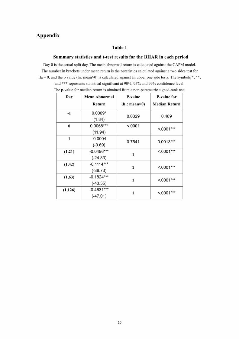
Table 1 Here

In table 1 we listed the summary statistics and t-test results for the BHARs. The mean

abnormal return is positive for the day before actual split day (t=-1) and the actual

split day (t=0), but it becomes statistically indifferent from 0 for t=1, and turns to

negative for t>1. The magnitudes for negative returns are large. The t-statistics shows

that other than t=1, the return numbers are statistically significant. We also applied a

non-parametric median test to test the robustness of the above results, and it supports

our results.

The abnormal return on actual split day supports the inattention theory, but the

negative returns after the actual split day remain a puzzle. Given the actual split does

not convey any new information, there should be little under- or over-reaction, thus

the abnormal return after the actual split day should remain close to zero. This review

is supported by Boehme and Danielsen (2007), who found that the abnormal return

after the announcement day failed to continue after the actual split day. Further

investigation thus is needed for the large negative abnormal returns after t=1.

3.3 Test for the influence from firm size, price before split and volume

From previous literatures we made some hypothesis for factors that may be associated

with abnormal return on actual split day. In this section we do some preliminary

analysis for each factor and get some intuition for the relationship.

 

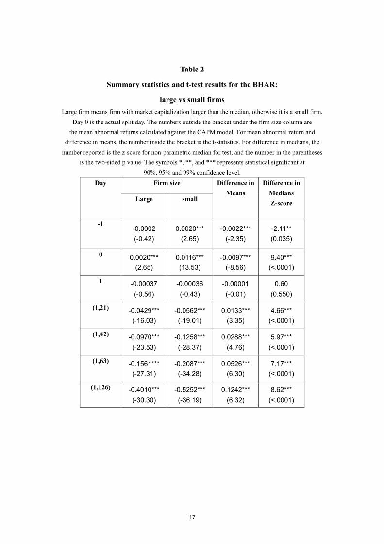
We first divided our data into two groups according to market capitalization on actual

split day. If a firm has market capitalization larger than the median, we define it as a

large capitalization firm; otherwise it is a small capitalization firm. Same statistics are

9 

calculated for the two groups. Table 2 shows the respective results.

Table 2 Here

Compared to large firm, small firm has higher mean abnormal return for t=-1 and t=0,

but lower mean negative abnormal return for the time period since t=1. The difference

in means and medians for the two groups on actual split day are also significant; the

robustness test (difference in medians) supports it as well. This result suggests that

firm size is negatively correlated with the abnormal return on actual split day. The

results are consistent with our secondary hypothesis.

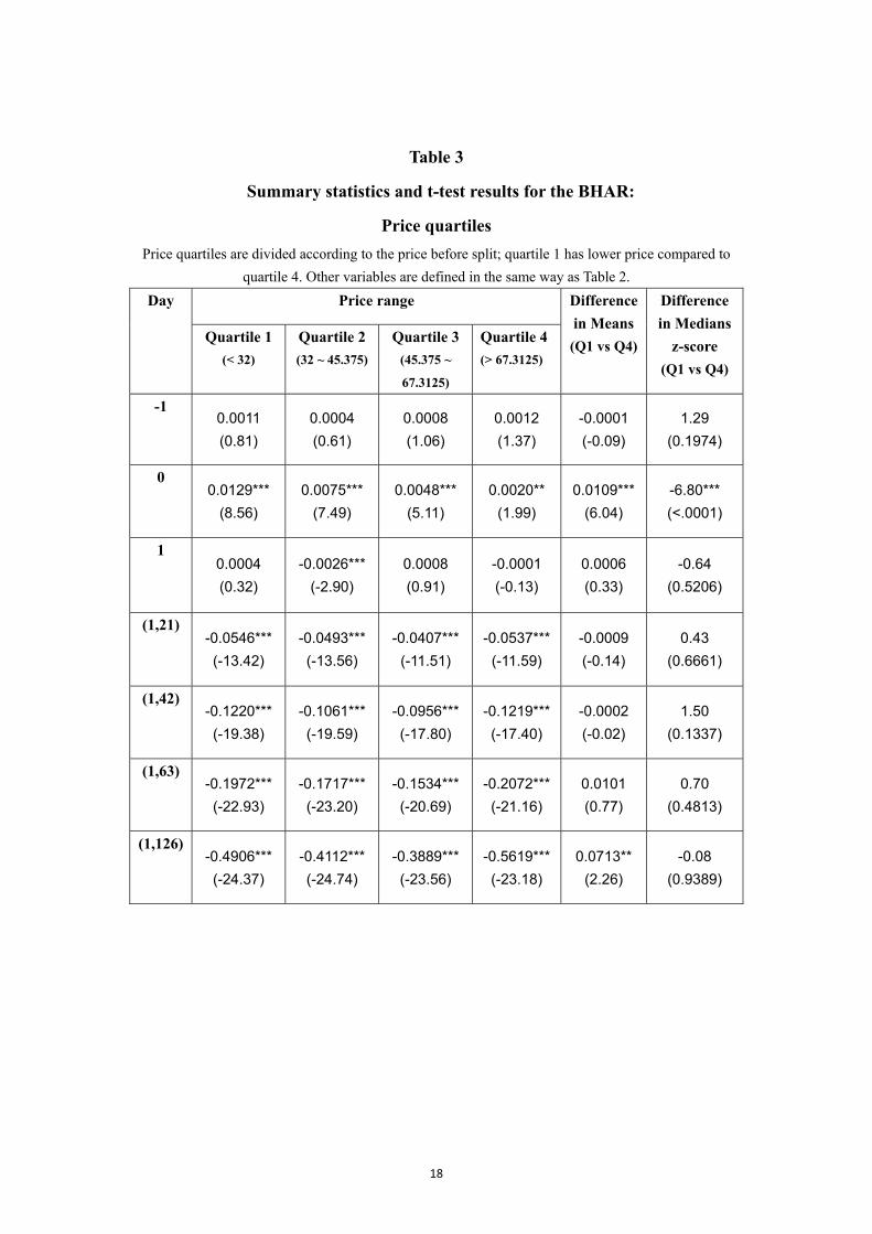
In terms of price, we rank the stocks according to their pre-split price. The mean price

is $55, median is $45.375, 75% quartile is $67.3125 and 25% quartile is $32. We

divide the stocks into four groups according to the quartiles, then compare their means

and medians. The results are summarized in table 3.

Table 3 Here

We observe some patterns for the mean abnormal return. On actual split day, the price

and mean abnormal return exhibits a negative relationship. As the price before split

increase from quartile 1 to quartile 3, the returns before t=1 decrease, but the returns

after t=1 have smaller negative values, which suggest that the quartile 3 firms have

smaller volatility compared to quartile 1 in terms of mean abnormal return. However,

firms in quartile 4 have abnormal return similar to quartile 1 after t=1, and we test the

difference in means and medians to confirm this result.

Above observations suggest that on actual split day, the mean abnormal return

decreases as price increase, which contradicts the optimal trading range hypothesis.

According to the optimal trading range theory, firms that have higher prices before

splits should receive more benefit from the split given their stocks are more affordable

to individual investors. Ikenberry et al (1996) also proposed that it would be costly for

10 

lower price stock to split because the fixed cost element of brokerage commissions

leads to a higher cost-per-share, which reduces the net benefit of splitting. Thus the

negative relationship seems counterintuitive, and we need regressions to prove

whether it is true.

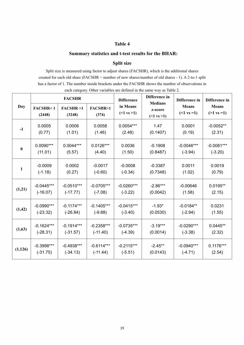
We also investigate if the stock with different split size has different mean abnormal

return. Here the factor to adjust shares (FACSHR) is used to measure split size, and it

is defined as the additional shares created after split for each old share.

1

For example, if the factor is 1 for the split, then it is a 2-to-1 split. The mean of

FACSHR of our sample is 0.89, median, mode and 75% quartile (even the 90%) are

both 1; the 25% quartile is 0.5. Thus most splits in the sample are 2-to-1 split.

We divided the data into three groups in terms of the FACSHR: (1) above 1; (2)

exactly 1; (3) below 1. Table 4 shows the results.

Table 4 Here

The return on actual split day shows a U-shape in terms of split size: the mean

abnormal return has the lowest value for FACSHR equals to 1(which is the mode,

more than 50% of our data have FACSHR of 1). For stocks with FACSHR larger than

1, its mean abnormal return has a value similar to that of stock with FACSHR smaller

than 1. The test of difference in mean as well as difference in median supports the

U-shape relationship on the actual split day. It seems market reacts more to splits with

less common split ratio. Further investigations are needed to explain the U-shape

relationship between mean abnormal return and split ratio.

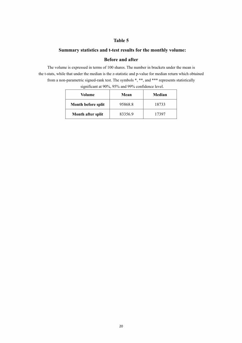
Finally, we collect monthly trading volume data before and after the split and study if

the stock split increase liquidity. The data are adjusted to reflect the equivalent

number of shares before the split. The results are summarized in Table 5.

11 

Table 5 Here

The mean and median monthly trading volume decrease after the split, implying that

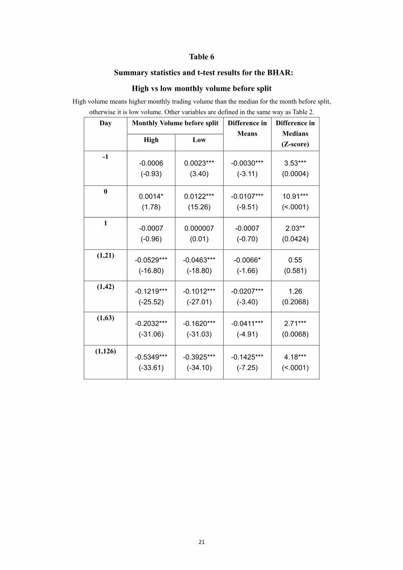
stock split decrease liquidity in the short term. We divide the stocks in two groups in

terms of trading volume one month before the split. If the volume is higher than the

median, it is defined as high volume, otherwise it is low. Table 6 is the result.

Table 6 Here

For stocks with lower trading volume before the split, the abnormal return is much

higher on actual split day, it is even positive on the day before split day (t=-1). The

difference in abnormal return between high and low trading volume is significant on

split day, and it passes robust test as well. From above results we infer that the mean

abnormal return on actual split day is negatively correlated with the trading volume

before split. The result is also consistent with our secondary hypothesis.

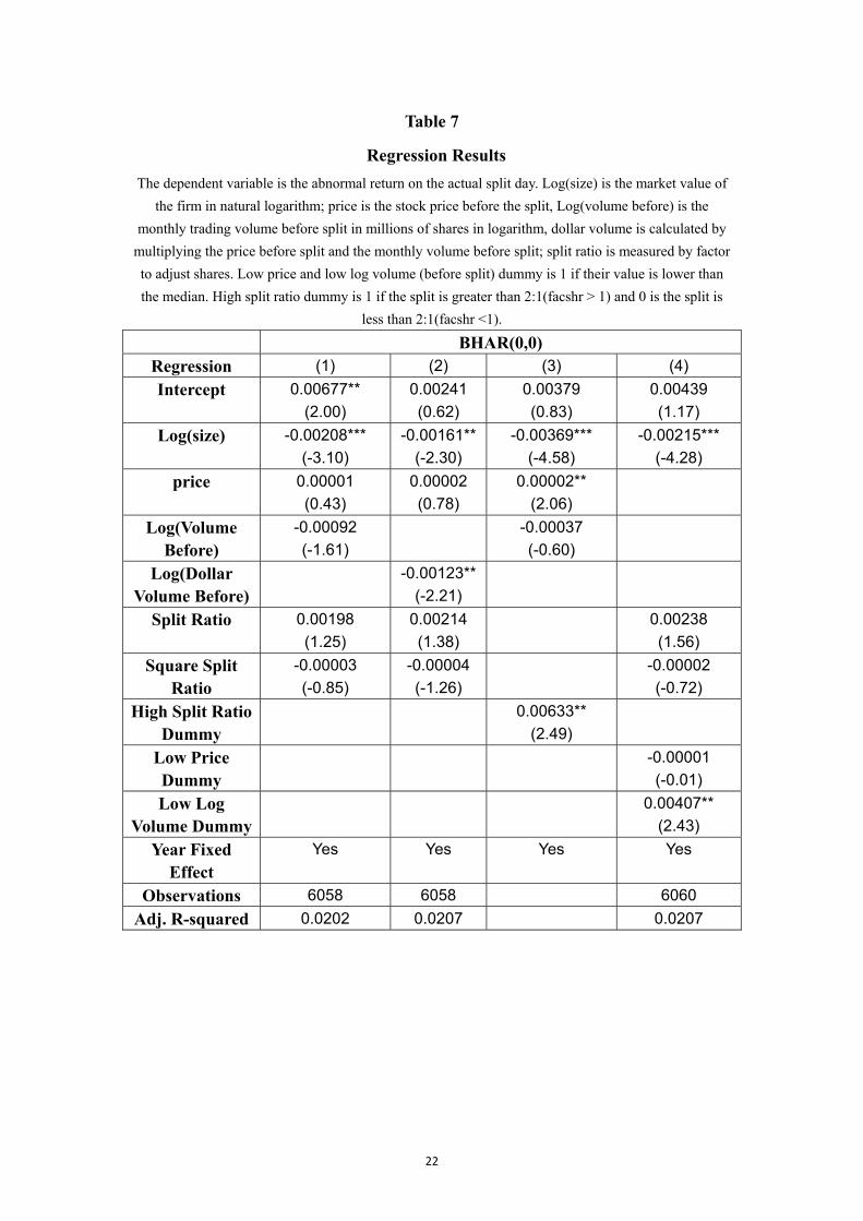
3.4 Regression

All above tables give us some clues for the influential factors of the abnormal return

on actual split day, thus next we do regressions to confirm whether these relationships

exist. We use the abnormal return at actual split day (bharMM0) as dependent

variables for all regressions, and vary the independent variables. We correct the

heteroscedasticity of errors by clustering by firms. Firm fixed effects are not

considered given there are too few splits per firm (3658 firms and 6062 splits) in our

sample, while year fixed effects are considered. Also, the split ratio (measured by

FACSHR) exhibits a U-shape relationship with abnormal return, we thus include both

split ratio and split ratio squared to avoid bias in linear coefficients. Since the variable

firm size, volume before split and dollar volume are highly skewed, we take their

natural log to make it more symmetric.

For the first two regressions, the independent variables are firm size (market

capitalization in trillions) in logarithm, price before split, monthly trading volume

12 

before split (in millions of shares) in logarithm, the split ratio (measured by factor to

adjust shares), squared split ratio, and dollar volume (monthly trading volume before

split in millions of shares times the price before split divided by 1000) in logarithm.

The result is in Table 7 regressions (1) and (2).

Table 8 Here

The size coefficient is highly significant and has negative sign, which is consistent

with the inattention theory as well as our hypothesis: larger firm that received less

attention on announcement day is associated with lower abnormal return on actual

split day. The volume coefficient is insignificant, but the log dollar volume coefficient

in regression (2) is negative and significant. The price coefficient is insignificant in

both the two regression.

In the univariate test of FACSHR (which measures split ratio), we found this variable

exhibits a U-shape relationship with the abnormal return on actual split day. In Table 7

regression (3) we create dummy for the less common splits in our sample: for stock

with split ratio higher than 2:1(FACSHR>1), the dummy is 1; if split ratio is lower

than 2:1 (FACSHR<1), the dummy is 0. The result shows that compared to stocks

with split ratio lower than 2:1, stocks with ratio higher than 2:1 will have on average

0.633% higher abnormal return on actual split day.

To further clarify if there are relationships between abnormal return and price as well

as log volume on actual split day, we create dummies for these two variables. If their

value is smaller than the median, the value of dummy will be 1; otherwise it is 0. The

result of this regression is in Table 7 regression (4).

The size still stays highly significant when dummies are applied. The log volume

dummy has positive coefficient and is significant, suggesting that firms with small

volume before split has abnormal return that is 0.411% higher than firms with larger

13 

volume. This is also consistent with the inattention theory. Firms that were ignored by

the market would tend to have a low volume before the split (or the opposite way:

firms have lower volume before the split have higher possibility to have inattention),

and Tables 6 and 7 show that these firms on average experience higher market

reaction to the split.

Finally, the price continues to be insignificant even when we create dummy; thus we

cannot find evidence to prove the optimal trading size hypothesis.

4 Conclusions

In this paper we examine the existence of abnormal return on the actual split day and

investigate factors that may contribute to the abnormal return, as well as theories that

are applicable to it. Through statistical analysis we found a negative relationship

between abnormal return and firm size as well as volume before split. The result

supports the inattention theory. However, we don’t find evidence in support of the

optimal trading range theory. The split ratio exhibits a U-shape relationship with

abnormal returns. We also found a large negative abnormal return after the actual split

day which is a puzzle. Further investigations are needed to address above two issues.

14 

References

Amihud, Y. and Mendelson, H. (1986), ‘‘Liquidity and stock returns’’, Financial

Analyst Journal, Vol. 42 No. 3, pp. 43-8.

Atiase, R(1985), Pre-disclosure information, firm capitalization, and the security price

behavior around earnings announcements. Journal of Accounting Research 23

(Spring): 21-36.

Brennan, M.J. and Copeland, T.E. (1988), Stock splits stock prices and transaction

costs, Journal of Financial Economics, Vol. 22, pp. 83-101. Desai, H and Jain P. C. (1997), Long-Run Common Stock Returns Following Stock

Splits and Reverse Splits. The Journal of Business, Vol. 70, No.3 (July 1997), pp.

409-433.

Gilbert, Thomas, Shimon Kogan, Lars Lochstoer, and Ataman Ozyildirim, 2012,

Investor Inattention and the Market Impact of Summary Statistics, Management

Science 58 (2), 336-350.

Ikenberry, D., Vermaelen T., 1996. The option to repurchase stock, Financial

Management 25, 9-24.

Kamoureux, C. and P. Poon. (1987). The Market Reaction to Stock Splits, Journal of

Finance, 42, 1347-70.

Lyroudi, K., Dasilas, A., & Varnas, A. (2006). The valuation effects of stock splits in

NASDAQ. Managerial Finance, 32(5), 401-419.

McNichols, M. and Dravid, A(1990). Stock dividends, stock splits, and signaling.

Journal of Finance 45(July): 857-79.

Muscarella, C. and Vetsuypens, M. (1996), ‘‘Stock splits: signaling or liquidity?’’,

Journal of Financial Economics, Vol. 42, pp. 3-26.

Mohammad. G Robbani (2014). The effect of stock split announcements on abnormal

returns during a financial crisis, Journal of Finance and Accountancy 15

2014-04-01 p1.

Rodney D. Boehme, Bartley R. Danielsen(2007), Stock-Split Post-Announcement

Returns: Underreaction or Market Friction? The Financial Review 42(2007)

485-506.

Raymond W. So, Yiuman Tse(2000), Rationality of Stock Splits: The Target-Price

Habit Hypothesis, Review of Quantitative Finance and Accounting

January 2000, Volume 14, Issue 1, pp 67-84

Said Elfakhani and Trevor Lung(2003), The effect of split announcements on

Canadian stocks, Global Finance Journal, Volume 14, Issue 2, July 2003, Pages

197–216

So,R., & Tse, Y. (2000). Rationality of stock splits: the Target-Price Habit Hypothesis.

Review of Quantitative Finance and Accounting, 14, 67-84.

15 

Xiaoqi Li, Philip Stork, Liping Zou (2013), An Empirical Note on US Stock Split

Announcements, 2000-2009, International Journal of Economic Perspectives.

Vol/Issue 7 (2), pp 41.

16 

Appendix

Table 1

Summary statistics and t-test results for the BHAR in each period

Day 0 is the actual split day. The mean abnormal return is calculated against the CAPM model.

The number in brackets under mean return is the t-statistics calculated against a two sides test for

H0 = 0, and the p value (h1: mean>0) is calculated against an upper one side tests. The symbols *, **,

and *** represents statistical significant at 90%, 95% and 99% confidence level.

The p-value for median return is obtained from a non-parametric signed-rank test.

Day Mean Abnormal

Return

P-value

(h1: mean>0)

P-value for

Median Return

-1 0.0009*

(1.84) 0.0329 0.489

0 0.0068***

(11.94)

<.0001 <.0001***

1 -0.0004

(-0.69) 0.7541 0.0013***

(1,21) -0.0496***

(-24.83) 1

<.0001***

(1,42) -0.1114***

(-36.73) 1 <.0001***

(1,63) -0.1824***

(-43.55) 1 <.0001***

(1,126) -0.4631***

(-47.01) 1 <.0001***

17 

Table 2

Summary statistics and t-test results for the BHAR:

large vs small firms

Large firm means firm with market capitalization larger than the median, otherwise it is a small firm.

Day 0 is the actual split day. The numbers outside the bracket under the firm size column are

the mean abnormal returns calculated against the CAPM model. For mean abnormal return and

difference in means, the number inside the bracket is the t-statistics. For difference in medians, the

number reported is the z-score for non-parametric median for test, and the number in the parentheses

is the two-sided p value. The symbols *, **, and *** represents statistical significant at

90%, 95% and 99% confidence level.

Day Firm size Difference in

Means

Difference in

Medians

Z-score

Large small

-1 -0.0002

(-0.42)

0.0020***

(2.65)

-0.0022***

(-2.35)

-2.11**

(0.035)

0 0.0020***

(2.65)

0.0116***

(13.53)

-0.0097***

(-8.56)

9.40***

(<.0001)

1 -0.00037

(-0.56)

-0.00036

(-0.43)

-0.00001

(-0.01)

0.60

(0.550)

(1,21) -0.0429***

(-16.03)

-0.0562***

(-19.01)

0.0133***

(3.35)

4.66***

(<.0001)

(1,42) -0.0970***

(-23.53)

-0.1258***

(-28.37)

0.0288***

(4.76)

5.97***

(<.0001)

(1,63) -0.1561***

(-27.31)

-0.2087***

(-34.28)

0.0526***

(6.30)

7.17***

(<.0001)

(1,126) -0.4010***

(-30.30)

-0.5252***

(-36.19)

0.1242***

(6.32)

8.62***

(<.0001)

18 

Table 3

Summary statistics and t-test results for the BHAR:

Price quartiles

Price quartiles are divided according to the price before split; quartile 1 has lower price compared to

quartile 4. Other variables are defined in the same way as Table 2.

Day Price range Difference

in Means

(Q1 vs Q4)

Difference

in Medians

z-score

(Q1 vs Q4)

Quartile 1

(< 32)

Quartile 2

(32 ~ 45.375)

Quartile 3

(45.375 ~

67.3125)

Quartile 4

(> 67.3125)

-1 0.0011

(0.81)

0.0004

(0.61)

0.0008

(1.06)

0.0012

(1.37)

-0.0001

(-0.09)

1.29

(0.1974)

0 0.0129***

(8.56)

0.0075***

(7.49)

0.0048***

(5.11)

0.0020**

(1.99)

0.0109***

(6.04)

-6.80***

(<.0001)

1 0.0004

(0.32)

-0.0026***

(-2.90)

0.0008

(0.91)

-0.0001

(-0.13)

0.0006

(0.33)

-0.64

(0.5206)

(1,21) -0.0546***

(-13.42)

-0.0493***

(-13.56)

-0.0407***

(-11.51)

-0.0537***

(-11.59)

-0.0009

(-0.14)

0.43

(0.6661)

(1,42) -0.1220***

(-19.38)

-0.1061***

(-19.59)

-0.0956***

(-17.80)

-0.1219***

(-17.40)

-0.0002

(-0.02)

1.50

(0.1337)

(1,63) -0.1972***

(-22.93)

-0.1717***

(-23.20)

-0.1534***

(-20.69)

-0.2072***

(-21.16)

0.0101

(0.77)

0.70

(0.4813)

(1,126) -0.4906***

(-24.37)

-0.4112***

(-24.74)

-0.3889***

(-23.56)

-0.5619***

(-23.18)

0.0713**

(2.26)

-0.08

(0.9389)

19 

Table 4

Summary statistics and t-test results for the BHAR:

Split size

Split size is measured using factor to adjust shares (FACSHR), which is the additional shares

created for each old share (FACSHR = number of new shares/number of old shares - 1). A 2-to-1 split

has a factor of 1. The number inside brackets under the FACSHR shows the number of observations in

each category. Other variables are defined in the same way as Table 2.

Day

FACSHR Difference

in Means

(<1 vs >1)

Difference in

Medians

z-score

(<1 vs >1)

Difference in

Means

(<1 vs =1)

Difference in

Means

(>1 vs =1) FACSHR< 1

(2448)

FACSHR =1

(3248)

FACSHR>1

(374)

-1 0.0005

(0.77)

0.0006

(1.01)

0.0058

(1.46)

0.0054***

(2.48)

1.47

(0.1407)

0.0001

(0.19)

-0.0052**

(2.31)

0 0.0090***

(11.01)

0.0044***

(5.57)

0.0126***

(4.40)

0.0036

(1.50)

-0.1908

(0.8487)

-0.0046***

(-3.94)

-0.0081***

(-3.20)

1 -0.0009

(-1.18)

0.0002

(0.27)

-0.0017

(-0.60)

-0.0008

(-0.34)

-0.3387

(0.7348)

0.0011

(1.02)

0.0019

(0.79)

(1,21) -0.0445***

(-16.07)

-0.0510***

(-17.77)

-0.0705***

(-7.08)

-0.0260***

(-3.22)

-2.86***

(0.0042)

-0.00646

(1.58)

0.0195**

(2.15)

(1,42) -0.0990***

(-23.32)

-0.1174***

(-26.84)

-0.1405***

(-9.88)

-0.0415***

(-3.40)

-1.93*

(0.0530)

-0.0184**

(-2.94)

0.0231

(1.55)

(1,63) -0.1624***

(-28.31)

-0.1914***

(-31.57)

-0.2358***

(-11.40)

-0.0735***

(-4.39)

-3.19***

(0.0014)

-0.0290***

(-3.38)

0.0445**

(2.32)

(1,126) -0.3998***

(-31.75)

-0.4938***

(-34.13)

-0.6114***

(-11.44)

-0.2115***

(-5.51)

-2.45**

(0.0143)

-0.0940***

(-4.71)

0.1176***

(2.54)

20 

 

Table 5

Summary statistics and t-test results for the monthly volume:

Before and after

The volume is expressed in terms of 100 shares. The number in brackets under the mean is

the t-stats, while that under the median is the z-statistic and p-value for median return which obtained

from a non-parametric signed-rank test. The symbols *, **, and *** represents statistically

significant at 90%, 95% and 99% confidence level.

Volume Mean Median

Month before split 95868.8 18733

Month after split 83356.9 17397

 

21 

Table 6

Summary statistics and t-test results for the BHAR:

High vs low monthly volume before split

High volume means higher monthly trading volume than the median for the month before split,

otherwise it is low volume. Other variables are defined in the same way as Table 2.

Day Monthly Volume before split Difference in

Means

Difference in

Medians

(Z-score) High Low

-1 -0.0006

(-0.93)

0.0023***

(3.40)

-0.0030***

(-3.11)

3.53***

(0.0004)

0 0.0014*

(1.78)

0.0122***

(15.26)

-0.0107***

(-9.51)

10.91***

(<.0001)

1 -0.0007

(-0.96)

0.000007

(0.01)

-0.0007

(-0.70)

2.03**

(0.0424)

(1,21) -0.0529***

(-16.80)

-0.0463***

(-18.80)

-0.0066*

(-1.66)

0.55

(0.581)

(1,42) -0.1219***

(-25.52)

-0.1012***

(-27.01)

-0.0207***

(-3.40)

1.26

(0.2068)

(1,63) -0.2032***

(-31.06)

-0.1620***

(-31.03)

-0.0411***

(-4.91)

2.71***

(0.0068)

(1,126) -0.5349***

(-33.61)

-0.3925***

(-34.10)

-0.1425***

(-7.25)

4.18***

(<.0001)

22 

Table 7

Regression Results

The dependent variable is the abnormal return on the actual split day. Log(size) is the market value of

the firm in natural logarithm; price is the stock price before the split, Log(volume before) is the

monthly trading volume before split in millions of shares in logarithm, dollar volume is calculated by

multiplying the price before split and the monthly volume before split; split ratio is measured by factor

to adjust shares. Low price and low log volume (before split) dummy is 1 if their value is lower than

the median. High split ratio dummy is 1 if the split is greater than 2:1(facshr > 1) and 0 is the split is

less than 2:1(facshr <1).

BHAR(0,0) Regression (1) (2) (3) (4)

Intercept 0.00677**

(2.00)

0.00241

(0.62)

0.00379

(0.83)

0.00439

(1.17)

Log(size) -0.00208***

(-3.10)

-0.00161**

(-2.30)

-0.00369***

(-4.58)

-0.00215***

(-4.28)

price 0.00001

(0.43)

0.00002

(0.78)

0.00002**

(2.06)

Log(Volume Before)

-0.00092

(-1.61)

-0.00037

(-0.60)

Log(Dollar Volume Before)

-0.00123**

(-2.21)

Split Ratio 0.00198

(1.25)

0.00214

(1.38)

0.00238

(1.56)

Square Split Ratio

-0.00003

(-0.85)

-0.00004

(-1.26)

-0.00002

(-0.72)

High Split Ratio Dummy

0.00633**

(2.49)

Low Price Dummy

-0.00001

(-0.01)

Low Log Volume Dummy

0.00407**

(2.43)

Year Fixed Effect

Yes Yes Yes Yes

Observations 6058 6058 6060

Adj. R-squared 0.0202 0.0207 0.0207