informed trading around stock split announcements ... annual meetings/2015-amsterdam...informed...

Informed trading around stock split announcements: Evidence from the

option market

Philip Gharghori*a, Edwin D. Maberlya and Annette Nguyenb

a Department of Banking and Finance, Monash University, Melbourne

3800, Australia

b Department of Finance, Deakin University, Melbourne 3125, Australia

*Corresponding author, phone: +61 3 9905 9247, email: [email protected]

2

Informed trading around stock split announcements: Evidence from the

option market

Abstract

Prior research shows that splitting firms earn positive abnormal returns and that they experience an

increase in stock return volatility. If they do, then the option market is an ideal venue to capitalize

on this information. By examining option-implied volatility, we assess option traders’ perceptions

on return and volatility changes arising from stock splits. We find that they do expect higher

volatility following splits. There is only weak evidence though of option traders anticipating an

abnormal increase in stock prices. In further analysis where we examine cross-sectional variation

in the option-implied volatility of splitting firms, we show that our option measures can predict

both stock volatility levels and changes after the announcement. However, there is little evidence

that they can predict the returns of splitting firms.

Key words: option traders, implied volatility, event study

JEL Classification: G11, G12, G13 and G14

3

1. Introduction

The option market is a venue for informed trading. Prior research has identified a number of reasons

why informed investors may prefer to trade equity options rather than the underlying stock. Such

reasons include higher leverage and ease of shorting (Black (1975)). An impressive amount of

recent empirical work has demonstrated evidence of informed trading in options for both the cross-

section of stocks and around firm specific events. Research that considers the cross-section of

stocks includes Cremers and Weinbaum (2010), Roll, Schwartz and Subrahmanyam (2010), Xing,

Zhang and Zhao (2010), Johnson and So (2012) and An, Ang, Bali and Cakici (2014). Earnings

announcements are studied by Diavatopoulos et al. (2012), Jin, Livnat and Zhang (2012) and

Atilgan (2014). Lastly, Hayunga and Lung (2014) and Lung and Xu (2014) consider analyst

recommendations and Chan, Ge and Lin (2014) examine M&As.

We contribute to this literature by investigating informed trading in options around stock

split announcements. There are two key reasons why stock splits are a particularly interesting event

to examine in the context of informed trading. First, unlike for example earnings announcements,

which are scheduled events, stock splits announcements are unanticipated events that the market

should not be aware of in advance. This allows us to more cleanly analyze whether informed option

investors are trading in anticipation of the impending event. Second, prior research shows that

stocks experience changes in both the level of their returns and the volatility of their returns due to

splits. This provides us with a novel opportunity to examine the expectations of option traders on

both return and volatility changes arising from the same event.

The specific observations of prior research on return and volatility changes due to splits

that inform our analysis are as follows. There is, on average, a strong positive reaction when firms

announce splits (Grinblatt, Masulis and Titman (1984), Chern, Tandon, Yu and Webb (2008) and

Lin, Singh and Yu (2009)). Positive return drift that lasts at least one year after the split

4

announcement is observed (Ikenberry, Rankine and Stice (1996), Desai and Jain (1997) and

Ikenberry and Ramnath (2002)). However, this drift is conditional on the period examined (Byun

and Rozeff (2003)) and it is driven by the relatively short period between the split announcement

date and the split effective date (Boehme and Danielsen (2007)). Stock volatility increases when

splits are announced (Ohlson and Penman (1985)), which is a common occurrence for any

unscheduled and meaningful corporate announcement. Finally, there is an increase in stock

volatility after splits are effected (Ohlson and Penman (1985), Dravid (1987) and Koski (1998)).

We examine option-implied volatility around 1,780 stock split announcements for the

period 1998 to 2012. We draw inference on option traders’ perceptions on volatility changes when

splits are announced and after they are effected, and on split announcement returns and longer-term

return drift following announcements. We document a consistent increase in implied volatility for

the most speculative short-dated options in the days preceding the split announcement. This is

indicative of informed trading in options. More pointedly, it suggests that news about impending

split announcements has leaked and that option investors are trading on this information. Implied

volatility increases in both call and put options, which indicates that the trading is driven by an

expected increase in stock volatility on and soon after the announcement. In contrast, if the increase

in implied volatility was only observed in calls, this would imply a directional bet on positive

announcement returns. After a large and expected increase in implied volatility on the

announcement date, implied volatility increases again on the next day but only in long maturity

options that expire after the effective date. This suggests that option traders expect that stock

volatility will increase after splits are effected.

To examine option traders’ expectations on return changes arising from splits, we employ

the option-implied volatility spread (Cremers and Weinbaum (2010)) and skew (Xing, Zhang and

Zhao (2010)). The spread and skew measure differences in implied volatility between suitably

5

matched calls and puts. In the days preceding the announcement, there is little in our results to

suggest that option investors are trading to exploit the well documented positive returns when splits

are announced. Given that our earlier analysis is strongly suggestive of volatility trading prior to

the announcement, we surmise that the announcement returns are not large enough to induce them

to trade. After splits are announced, there is some evidence of option trading in anticipation of

longer-term return drift, particularly in smaller stocks, but the findings are not compelling.

The analysis discussed thus far focuses on the perceptions of option investors on return and

volatility changes due to splits. We also assess informed trading in options by examining whether

various implied volatility measures can predict future stock returns and volatility. In cross-sectional

regressions of abnormal stock volatility on daily changes in implied volatility prior to the

announcement, we show that implied volatility changes significantly predict the level of stock

volatility on the day after the announcement. Thus, not only do option traders seem to be trading

in anticipation of volatility increases due to split announcements, they also demonstrate an ability

to predict stock volatility levels after the announcement. More broadly, in addition to displaying a

capacity to acquire information, option traders also appear to be processing information skillfully.

We next show that the change in implied volatility from the announcement day to the

following day significantly predicts which splitters will have the largest change in stock volatility

after splits are effected – where the effective date is on average 40 days after the announcement

date. An informed traders’ private informational advantage is likely to be low directly after major

news announcements. Thus, we contend that this specific instance of informed trading highlights

option traders’ superior ability to process public information. Finally, we run similar regressions

to Jin, Livnat and Zhang (2012) and Chan, Ge and Lin (2014) where we examine whether the

implied volatility spread and skew predict short-run announcement returns and longer-term

6

abnormal returns. We find little evidence that these option measures can predict the future returns

of splitters.

Our paper makes several contributions to the literature. The prior research on informed

trading in options around corporate events focuses on the predictability of option measures and in

particular, predictability on future returns (for example, Jin, Livnat and Zhang (2012), Chan, Ge

and Lin (2014) and Hayunga and Lung (2014)). We are the first to examine the expectations of

option traders on both return and volatility changes due to an unscheduled corporate event. More

broadly, once could argue that this is the first paper that explicitly focuses on option traders’

perceptions of a corporate event. Another key contribution is that we develop tests that disentangle

option traders’ expectations on return and volatility changes, so that we can draw inference on

each. When analyzing predictability, our novel contribution is to evaluate whether option measures

can predict both the level and change of future stock volatility due to the event. By investigating

both the perceptions of option traders and predictability in options trading, we assess both the

acquisition and skillful processing of information. This allows us to present a more complete

picture of informed trading in options.

We find that informed option traders demonstrate an ability to acquire and skillfully

interpret information prior to the event. This contributes to the body of literature that documents

informed trading in options prior to other corporate events (for example, Chan, Ge and Lin (2014)

and Hayunga and Lung (2014)). We also complement research that shows pre-event informed

trading by other market participants such as investment banks (Bodnaruk, Massa and Simonov

(2009)), short sellers (Karpoff and Lou (2010)), institutional investors (Ivashina and Sun (2011))

and hedge funds (Massoud, Nandy, Saunders and Song (2011)). After the announcement, we show

that informed option traders possess a superior ability to process public information. This builds

on similar recent evidence with options on other corporate events (Jin, Livnat and Zhang (2012))

7

and with short sellers using broader news announcements (Engelberg, Reed and Ringgenberg

(2012)).

In the context of prior research on splits, rather than focusing on the return distribution of

splitting stocks as the majority of prior studies have done1, we contribute to this literature by

assessing the perceptions of informed option traders. Our tests are quite simple and given that they

focus on the expectations of option investors, we believe that they are more forward looking than

conventional event study tests, which rely on stock returns.

The rest of the paper proceeds as follows. Section 2 outlines the research design. Section 3

discusses data, sample selection and sample characteristics. Section 4 presents the findings of the

perceptions analysis. Section 5 reports on the predictability analysis. Section 6 concludes.

2. Research design

The initial analysis considers option traders’ perceptions on future return and volatility changes

due to splits. To investigate their perceptions on stock volatility, we examine the implied volatility

of call and put options separately. With future return changes, we analyze the implied volatility of

call and put options together by examining the volatility spread and skew. Our event window is the

[-5, +5] day period around the split announcement.

In these tests, we examine the daily change in implied volatility, and the volatility spread

and skew. Given that volatility is persistent, implied volatility today is an appropriate proxy for

1 There have been three published papers on stock splits and the option market, each of limited scale and scope. Reilly

and Gustavson (1985) find that call option returns are positive prior to split announcements but negligible post

announcement. French and Dubosfky (1986) observe that the implied volatility of call options increases after the

effective date but that high bid-ask spreads would render a trading strategy based on this increase unprofitable. Sheikh

(1989) also finds that call option-implied volatility increases when splits are effected but that this increase was not

anticipated at the time of the announcement. These studies spanned the period 1976 to 1983 and Sheikh’s (1989)

sample was the largest with 83 stocks.

8

expected implied volatility tomorrow. If the volatility spread and skew are indicators of future stock

returns, in the absence of new information, these measures should be constant through time. Thus,

we assume that the expected daily change in implied volatility and the volatility spread (skew) is

zero. Our approach is consistent with Bollen and Whaley (2004) and Garleanu, Pedersen and

Poteshman (2009) who find that changes in implied volatility reflect the net buying pressure of

option investors.

2.1 Testing perceptions on volatility

Ohlson and Penman (1985) document a temporary increase in stock volatility after the split

announcement and a more permanent increase after splits are effected. In the days preceding the

announcement, if informed option traders are speculating on a volatility spike when splits are

announced, then it is likely that they will employ shorter maturity options to do so2. When firms

announce splits, they will disclose on what date the split will be effected. If option traders expect

stock volatility to change after the effective date, then post-announcement, the behavior of implied

volatility should differ depending on whether the options expire before or after the effective date.

Accordingly, we compute the implied volatility for options that expire before and after the effective

date, separately. Furthermore, if option investors are trading in anticipation of a change in the

volatility of the underlying stock, then they will likely select options that are the most sensitive to

changes in stock volatility. That is, options with the highest vega. Thus, to obtain a single estimate

of option-implied volatility for a given stock, we take the weighted average of all available implied

volatilities where the weight is the option vega.

2 Short-dated options are more exposed to changes in short-term volatility, as the mean-reversion in stock volatility

results in the implied volatility of long-dated options being more stable. Moreover, the option gamma, which reflects

jump risk(s), is greatest for short dated options.

9

To examine option traders’ expectations on future stock volatility, we calculate the daily

change in implied volatility for call and put options as follows:

. (1)

is the change in implied volatility for stock i on day t and is the weighted average of all

implied volatilities for stock i on day t where the weight is the option vega. It is calculated as:

,

, ,

1

i tN

i i

it j t j t

j

IV w IV

, (2)

where ,i tN is the number of options traded for stock i on day t and i

tjIV , is the implied volatility of

option j for stock i on day t. Thus, we study the daily movement in the aggregate implied volatility

across all options for a given stock.

2.2 Testing perceptions on returns

Although option-implied volatility reflects the demand of option investors, it may not be a reliable

predictor of future stock returns. An increase in option-implied volatility may simply be the result

of an expected increase in the volatility of the underlying stock. Recent literature including Cremers

and Weinbaum (2010) and Xing, Zhang and Zhao (2010) suggest that the behavior of implied

volatilities of call and put options together, not in isolation, reflect informed trading and predict

returns in the equity market. Specifically, Cremers and Weinbaum (2010) argue that if informed

investors are optimistic about the underlying stock, then they can either buy a call option or sell a

put option. This should increase (decrease) the price of call (put) options, which in turn induces a

higher implied volatility inverted from call options relative to put options. They refer to this as the

volatility spread.

The change in the volatility spread is calculated as follows:

1 ititit IVIVIV

itIV itIV

10

. (3)

Following Cremers and Weinbaum (2010), the volatility spread for firm i on day t is:

= puti

tj

calli

tj

N

j

i

tj IVIVwti

,

,

,

,

1

,

,

, (4)

where j represents each pair of call and put options matched on the same strike price and maturity

date, and refers to the number of valid pairs of options on stock i. We eliminate option pairs

when either the call or put has zero open interest or a bid price of zero. The volatility spread for a

given firm is computed by taking the weighted average of all the available option pairs where the

weight is the average open interest in the call and put options (Cremers and Weinbaum (2010)).

In addition to the volatility spread, we employ the volatility skew measure developed by

Xing, Zhang and Zhao (2010). Unlike the volatility spread, which is designed to capture

information in a wide range of options across different strike prices and time to maturities, the

option-implied volatility skew specifically captures information in out-of-the-money put options.

The volatility skew is calculated as the difference in implied volatility between out-of-the-money

put options and at-the-money call options. Doran, Peterson and Tarrant (2007) and Xing, Zhang

and Zhao (2010) show that an increase in demand for out-of-the-money put options relative to at-

the-money call options predicts negative stock returns. Jin, Livnat and Zhang (2012) and Chan, Ge

and Lin (2014) find that the volatility skew forecasts positive returns as well.

If option traders believe in the existence of positive abnormal returns subsequent to the split

announcement, then we should observe a reduction in the volatility skew over the event window.

The volatility skew is estimated as follows:

, (5)

1 ititit VSVSVS

itVS

puts

ti

calls

tiit IVIVVS ,,

tiN ,

ATMC

ti

OTMP

titi IVIVSKEW ,,,

11

where is the option-implied volatility skew for stock i on day t, is the implied

volatility of out-of-the-money put options for stock i on day t, and is the implied volatility

of at-the-money call options for stock i on day t. Following Jin, Livnat and Zhang (2012), we select

out-of-the-money put options by first identifying options that have a delta within the range [-0.45,

-0.15] and choose the one that has a delta closest to -0.3. At-the-money call options are those whose

delta is closest to 0.5 given that delta is higher than 0.4 and less than 0.7. In this case, as only one

call and put is chosen per day for each splitting firm, no weighting is required. Similar to the

volatility spread, we examine the change in the volatility skew. That is,

1 ititit SKEWSKEWSKEW . (6)

2.3 Testing the predictive ability of option measures

For the predictability analysis, we run cross-sectional regressions of various option measures on

future stock returns and volatility. We assess whether these option measures can predict stock

volatility at the announcement and the change in volatility after the effective date. We also test

whether they can predict the announcement returns and returns in the post-announcement period.

To examine whether option-implied volatility can predict stock volatility at the

announcement, we run the following regression:

.i i iAbVol Intercept IV (7)

AbVoli is abnormal stock volatility and is estimated as the square of the daily returns on Day 0 or

Day +1 minus the average squared returns over the [-60, -20] period. iIV is the daily change in

implied volatility in the pre-announcement period, as defined in equation (1). In the absence of new

information and given the persistence in volatility, the daily change in implied volatility should

tiSKEW,OTMP

tiIV ,

ATMC

tiIV ,

12

have no predictive power in a cross-sectional analysis. Thus, this regression allows us to test for

informed option trading on stock volatility levels after the announcement.

The regression analyzing the predictability of changes in stock volatility after the effective

date is:

, , .post effective i pre effective i i iIntercept IV (8)

The post-effective change in volatility is measured as the difference in the annualized standard

deviation of the daily returns following the effective date ( post effective ) and the annualized standard

deviation of the daily returns from the announcement date to the effective date ( pre effective ). The

number of days for which the post-split volatility is calculated is equivalent to the number of days

from the announcement date to the effective date. Given that the date on which the split is effected

is announced at the same time the split is, we consider changes in implied volatility on the

announcement date and the following few days. Thus, we are examining whether option traders

skillfully process the information in the announcement on post-split changes in stock volatility.

As implied volatility is considered a forecast of stock volatility over the life of the option,

it would be inappropriate to conduct the predictability analysis on stock volatility using the daily

level of implied volatility. For our primary tests of the predictability of future returns though, we

use the daily level of the volatility spread and skew. This is consistent with the main analyses

undertaken by Jin, Livnat and Zhang (2012) and Chan, Ge and Lin (2014).

To examine whether our option measures can predict the announcement returns, we

estimate the following regressions:

1

(0, 1) ,n

i i j ij i

j

CAR Intercept VS ControlVariables

(9)

13

1

(0, 1) .n

i i j ij i

j

CAR Intercept SKEW ControlVariables

(10)

CAR is the cumulative announcement abnormal return, VSi and SKEWi are as defined in equations

(4) and (5), and the control variables are described in Appendix 1. These regressions allows us to

test whether the level of the spread and skew in the days preceding the announcement explain the

announcement returns.

The final regressions we run consider the predictability of returns in the post-announcement

period:

1

( 7, 60) ,n

i i j ij i

j

BHAR Intercept VS ControlVariables

(11)

1

( 7, 60) .n

i i j ij i

j

BHAR Intercept SKEW ControlVariables

(12)

BHAR is the buy and hold abnormal return and the control variables are again listed in Appendix

13. As with the regressions on the post-split change in volatility, we analyze the spread and skew

on the announcement day and the following few days. In so doing, we assess option traders’ ability

to interpret the information in the split announcement on future return drift.

3. Data and sample characteristics

From the OptionMetrics Ivy database, equity option data are collected for the period January 1998

to December 2012. The dataset covers daily closing bid and ask quotes, open interest, volume,

implied volatility and the Greeks for all exchange-listed call and put options on U.S. equities. Since

options on individual stocks are American options, implied volatilities are calculated using the

3 The expected return used to calculate both the CAR and BHAR is the daily equal weighted return of the matching

size portfolio, where four size portfolios are formed based on NYSE rankings.

14

Cox-Ross-Rubinstein (1979) binomial tree model, taking into account discrete dividend payments

and the possibility of early exercise using historical LIBOR as the interest rate. Specifically,

different values of volatility are inserted into the model until the price of the option approximates

to the midpoint of the option’s best closing bid-ask prices.

The OptionMetrics data are merged with the CRSP files to identify all splitting stocks with

a split factor greater than or equal to 25% that have written options. In the period 1998 to 2012,

1,780 stock splits on 1,109 firms meet this requirement. With regard to the option data, each option

record must have information on the strike price, best closing bid and ask prices, volume, open

interest and implied volatility during the period [-10, +10] where Day 0 is the split announcement

date. To address the issues related to thinly traded options, we impose the following filters: (1)

options with an absolute value of delta less than 0.02 and more than 0.98 are excluded; (2) options

must have maturities that range between 10 to 100 days; (3) all options with a bid-ask spread that

is greater than the bid-ask mid-point are removed. There are on average 22 (23) call (put) options

available on each splitting firm.

3.1 Summary statistics on option liquidity and implied volatility

To draw an initial inference on how the option market behaves in a period outside the split

announcement window, the average implied volatility, volume and open interest of call/put options

across different levels of moneyness is examined for the 10 day period from [-60 to -50]. We

measure the degree of moneyness of an option using the option delta, which represents the risk-

neutral probability of the option being in-the-money at expiration. Table 1 reports the results.

[Insert Table 1 here]

There is a U-shaped volatility smile for both call and put options, as is typically observed.

We also see that out-of-the-money and near-the-money options tend to have higher volume and

15

open interest than in-the-money options. This is expected, as trading in the option market is

typically motivated by speculation or hedging. Since out-of/near-the-money options are relatively

cheaper, they offer investors a higher degree of leverage and a better means to achieve their

objective. This in turn makes out-of-/near-the money options more popular amongst investors

compared to in-the-money options. Finally, the median volume and open interest for both call and

put options are much lower than their means and in some cases equal to zero. This indicates that

trading activity in the option market is quite thin where a large fraction of the option trading volume

and open interest reside in the contracts of only a few stocks.

3.2 Summary statistics for market capitalization groups

Easley, O’Hara and Srinivas (1998) argue that informed investors’ decision to trade in the option

market depends on leverage and the liquidity of the option market relative to the stock market. The

advantage of a liquid market is that it offers lower trading costs and it allows informed investors to

hide their information. Another relevant consideration for informed investors when deciding

whether to trade options is the behavior of the market makers. When the market makers obtain

news, which they deem to have a material price impact, they will adjust the bid and ask prices in a

way that inhibits other informed traders from earning abnormal returns. Informed investors faced

with this situation can do one of the following. If they believe that abnormal returns cannot be

earned based on the current bid and ask prices, they will not trade. If they disagree with the market

makers, they can trade in the opposite direction. Finally, if they agree with the market makers and

they believe that abnormal returns can still be earned, their trades will drive the bid and ask prices

in the same direction initiated by the market makers. In this context, a significant change in implied

volatility or the volatility spread (skew) when option liquidity is low is more likely to reflect the

16

perception of the market makers4. Contrastingly, when option liquidity is high, changes in these

metrics are more likely to be driven by both the market makers and other informed option traders.

Thus, we contend that a significant change in implied volatility or the volatility spread (skew)

observed in liquid options is a stronger signal of informed investors’ perceptions compared with

illiquid options.

Option trading volume, open interest and bid-ask spreads are important elements of option

liquidity, but no single attribute adequately describes liquidity. Therefore, a proxy is required that

represents all three elements of option liquidity, and market cap is the proxy selected. The

classification scheme employed forms four size portfolios, where the first three groups comprise

firms that constitute the S&P 500, S&P 400 and S&P 600 indices while the last group includes

firms that do not belong to these three indices. Together, the three S&P indices constitute the S&P

1500 index, accounting for approximately 85% of U.S. market capitalization. In unreported results,

the average (median) market cap of stocks in the “other” portfolio is higher (lower) than for S&P

600 stocks. The reason for this is that although small firms dominate the “other” portfolio, this

group also contains a number of Nasdaq 100 stocks that are not members of the S&P 1500 Index.

By design, Nasdaq 100 firms have high market cap.

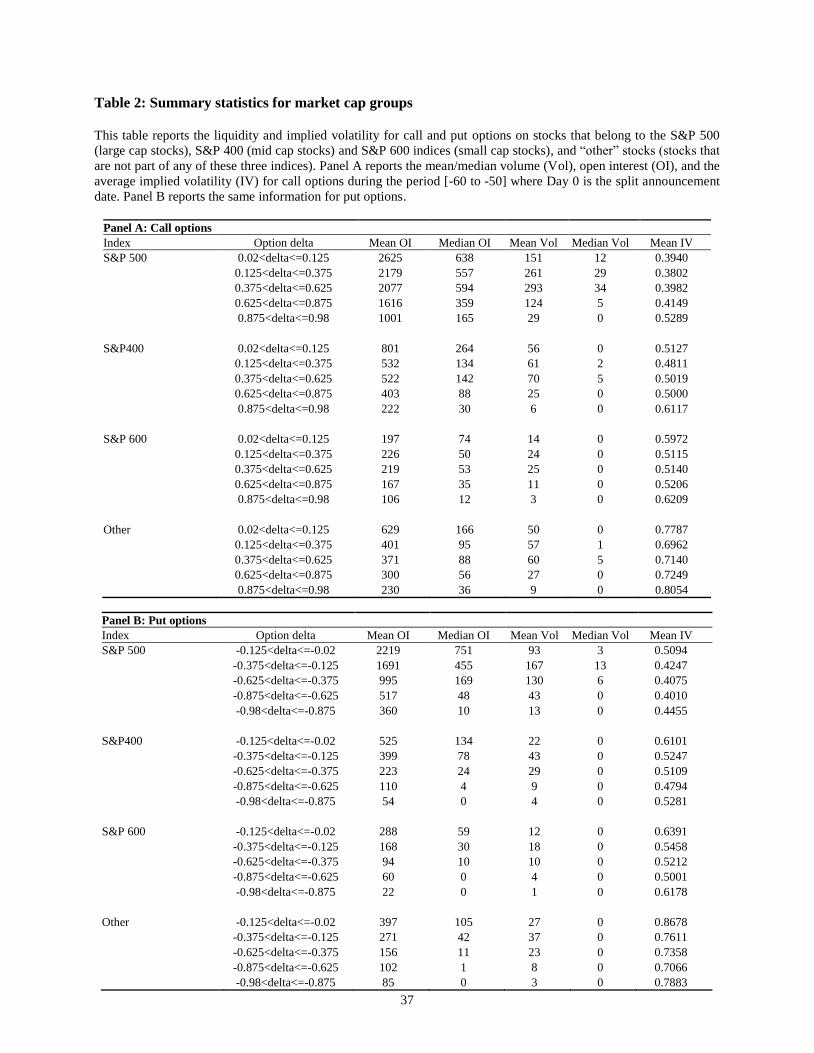
To evaluate whether market cap adequately captures option liquidity, an examination of

option trading volume and open interest is performed using options on stocks associated with the

four size portfolios, as previously identified. Table 2 documents the findings. Once again, we

observe a U-shaped volatility smile across all four capitalization groups. As for option liquidity,

there is a monotonic decline in the mean (median) option volume and open interest as one moves

4 Illiquid options suggest a low level of trading activity from option investors. This does not necessarily imply a high

degree of agreement between the market makers and other informed investors. The low trading activity may be due to

minimal interest by investors in the stock and its options.

17

from the large cap S&P 500 group to the small cap S&P 600 group. This pattern is present in both

call and put options, and at different moneyness levels. Option liquidity for stocks that belong to

the “other” group, as measured by the mean (median) trading volume and open interest, is higher

than in the S&P 600 index and marginally lower than in the S&P 400 index. The “other” portfolio

contains a number of higher capitalized Nasdaq 100 stocks, which exhibit high option liquidity.

This explains why the average liquidity of options for the “other” portfolio is higher than the S&P

600 portfolio and only slightly lower than the S&P 400 portfolio.


Overall, the results show that option liquidity is increasing in market cap, which supports

the use of market cap as a proxy for the level of option liquidity. In addition, stocks that constitute

the S&P 500 index not only exhibit the highest option liquidity compared to the other three size

groups, the mean (median) option trading volume and open interest for firms in this group is more

than triple that of the mid-cap S&P400 group. This is consistent with our earlier evidence that the

liquidity in the option market is concentrated in the contracts on a small proportion of stocks.

Another advantage of grouping stocks by market cap is that it allows us to assess the perceptions

of option traders in stocks that have varying levels of informational efficiency. As well as being

the most liquid, S&P500 stocks are also the most informationally efficient, so we are particularly

interested in the findings for this group.

3.3 Summary statistics on the volatility spread and skew

Next, we examine the volatility spread and skew over a short period preceding the split

announcement window. This forms the first reference point on which to base expectations on the

behavior of the volatility spread and skew. Table 3 reports the output. Similar to Cremers and

Weinbaum (2010) and Xing, Zhang and Zhao (2010), the mean and median volatility spread are

18

negative while for the volatility skew, these values are positive. This indicates that the implied

volatilities inverted from put options are relatively higher than those for call options, which reflects

option investors’ greater concern over downside risks. The findings for the different market cap

groups are broadly consistent with the full sample. However, it is observed that the absolute value

of the volatility spread and skew increases as market capitalization decreases. This implies that put

options are more expensive in small firms compared to large firms. This is expected, as smaller

firms are more likely to be subject to short-sale constraints, which leads to higher demand for put

options.


We also note that the absolute value of the volatility spread is lower than the volatility skew.

The volatility skew is designed to extract the information in out-of-the-money put options while

the volatility spread captures the information in both call and put options. If the difference in

implied volatility between call and put options is mainly driven by the put options, then the

magnitude of the volatility spread and skew should be similar, they should just have the opposite

sign. Thus, the lower absolute value of the volatility spread indicates that these spread differentials

are a function of price pressure in both calls and puts.

Overall, the summary statistics indicate that trading activity in the option market is quite

thin. Option liquidity does increase markedly though as one moves up through the market cap

groups. Moreover, without the effect of new information, the volatility spread and skew are not

centered on zero. Thus, to evaluate whether option traders expect positive abnormal returns

following stock split announcements, we do not study the level of the volatility spread and skew,

rather we examine the change in these two measures.

19

4. The perceptions of option traders

4.1 Perceptions on volatility

Table 4 reports implied volatility changes for both call and put options during the [-5, +5] event

window. Short (long) maturity options are those that expire before (after) the effective date. Prior

to the announcement, we observe significant increases in implied volatility in both short maturity

calls and puts. Specifically, there are significant increases on days -3, -2 and -1 in calls and on days

-2 and -1 in puts. There are also weakly significant increases on day -5 in calls and on day -4 in

puts. In contrast, long maturity options only exhibit a significant increase on day -2. As these

implied volatility increases are observed in both calls and puts but primarily in short maturity

options, they imply that option traders expect that stock volatility will increase when splits are

announced. Given that splits are unscheduled events that the market should not have foreknowledge

of, these findings are strongly suggestive of information leakage prior to the announcement.


On the announcement day and as expected, there is a very large increase in implied

volatility across all option groups. On day +1 though, there is a significant (small) reduction in

implied volatility for short maturity puts (calls). In contrast, both long maturity calls and puts

exhibit another significant increase in implied volatility on day +1. As this increase is observed in

both calls and puts but only in long maturity options, it suggests that option traders expect that

stock volatility will increase after the effective date. Given that these are post-announcement

changes, they incorporate option traders’ interpretation of the information in the event.

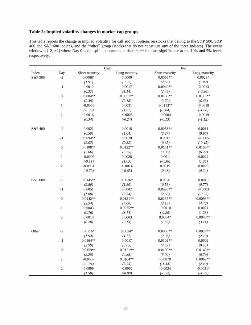
Table 5 presents the sub-sample analysis for the four market capitalization groups. The

daily change in implied volatility is only reported over the [-2, +2] period in order to conserve

20

space5. Across the four size groups, both the short maturity calls and puts consistently show a

significantly positive change in implied volatility on either day -2 or day -1, or on both days. Thus,

the pre-announcement increase in implied volatility documented in the full sample is also present

in each of the four size groups. This is a particularly strong result, as it indicates that stock volatility

is expected to increase across a broad cross-section of stocks, whose options will have varying

degrees of liquidity. The increase in implied volatility in S&P500 stocks is especially telling, as it

is more likely to be driven by completed trades rather than by market makers adjusting spreads to

inhibit the informed from profiting.


Unsurprisingly, in all market cap and option groups, there is a large and significant increase

in implied volatility on day 0. On the ensuing days though, the behavior of implied volatility varies

across the size groups. Specifically, we only observe a significant increase in implied volatility

after the announcement day for long maturity options in S&P 600 and “other” stocks. This suggests

that the inference reached from the full sample that option traders expect an increase in volatility

after the effective date manifests in smaller stocks. In un-tabulated results, the post-split change in

stock volatility, as defined in section 2.3, is 10.3% p.a. for the full sample. It is 5.4%, 7.0%, 13.3%

and 14.2% for S&P500, S&P400, S&P600 and “other” stocks, respectively. Thus, option traders’

expectation of a post-split increase in stock volatility, particularly in smaller stocks, is in line with

the actual increases observed.

If an informed investor wishes to trade on information they have acquired on an impending

event, when should they start trading to exploit that information? They will probably consider how

much trading they think they can get away with without showing their hand. They may trade by

5 Outside of the [-2, +2] window, that is for days -5, -4, -3, +3, +4 and +5, the change in implied volatility is insignificant

for all size groups.

21

stealth in smaller blocks (Anand and Chakravarty (2007)) over multiple days. It is also likely to

depend on the extent of information they have on the impending event. For example, they may

have foreknowledge of both the split announcement and when it will be made, perhaps they do not

know the exact date of the announcement, or maybe they know that some sort of meaningful

corporate announcement will be made in the near future. Regardless, it is unlikely that the

significant increases observed in implied volatility prior to the announcement are driven solely by

those with some form of inside information. Particularly given the illegality of this trading. At

some point, the informed trading by those with some knowledge of the impending split will

probably be detected by other informed traders. Once detected, market makers will likely adjust

spreads and other informed investors will consider jumping on the bandwagon. Our results show

that the critical mass in trading seems to occur a few days prior to the announcement, as this is

when implied volatility starts to significantly increase6.

This increase, which is detected in both short-dated calls and puts, indicates that option

traders expect stock volatility to increase post-announcement. Looking more closely though, we

see that the magnitude of the increase is larger in calls than puts. Specifically, in table 4, there is a

0.67%, 0.89% and 0.84% increase on days -3, -2 and -1 in calls compared with 0.19%, 0.50% and

0.67% for the corresponding days in puts. The greater buying pressure observed in calls could

imply not only an expectation of volatility increases but also of positive abnormal returns on the

announcement. In a similar fashion, table 4 shows that the implied volatility increase in long

maturity calls is 0.64% on day +1 compared with 0.26% in puts. This could suggest that there is an

6 It is possible that the observed implied volatility increases are not due to information leakage but are solely due to

superior processing of public information by informed traders. We think that this is unlikely though. Further, market

makers may adjust spreads as an informed reaction to suspicious trading or as part of their normal inventory

management processes. Even in the latter case though, the change in spreads will still have been initiated by informed

option trading.

22

expectation of both an increase in post-split volatility and of positive abnormal returns over the

longer-term. Therefore, we need to more carefully analyze whether changes in option-implied

volatility reflect a change in investors’ perceptions on the volatility or returns of the underlying

stock. This is especially pertinent given that An, Ang, Bali and Cakici (2014) find that changes in

implied volatility predict future returns. This leads to our next tests, which examine the volatility

spread and skew.

4.2 Perceptions on returns

To draw inference on option traders’ perceptions on return changes due to splits, we analyze the

change in the volatility spread and skew. Prior to the announcement, we are particularly interested

in these changes in short maturity options. There are two reasons for this. First, if option investors

are trading in anticipation of positive returns on the announcement, they are likely to employ

shorter-dated options. Second, in the preceding analysis, there were numerous instances where

implied volatility significantly increased in short maturity calls prior to day 0.

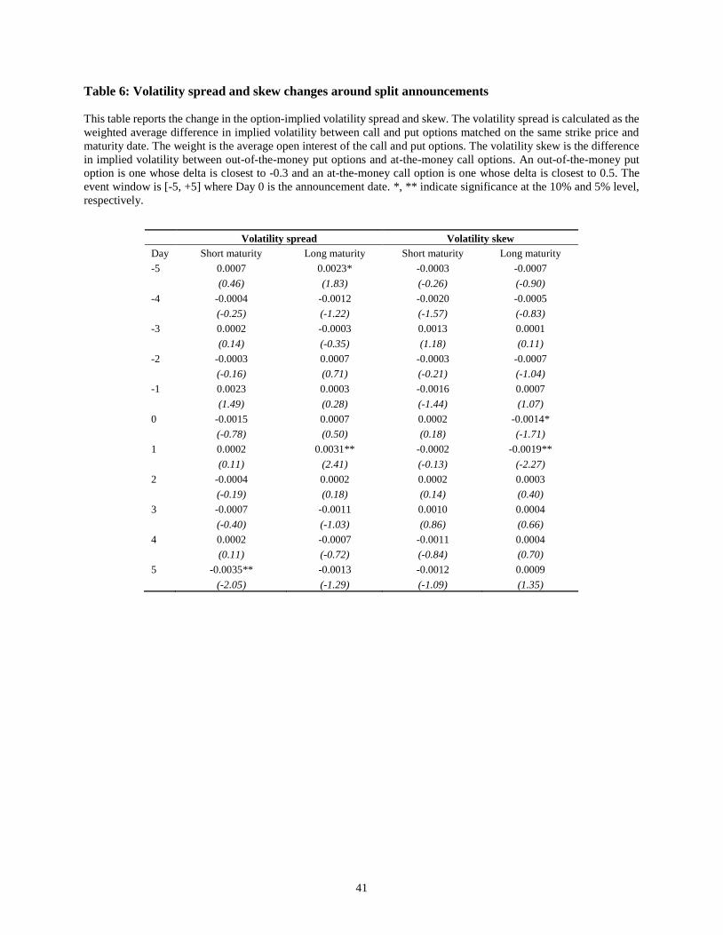
Table 6 shows that there are no significant changes in the volatility spread and skew prior

to the announcement in short maturity options. In fact, there is only one weakly significant change

observed prior to day 0 and this is on day -5 in long maturity options for the volatility spread. The

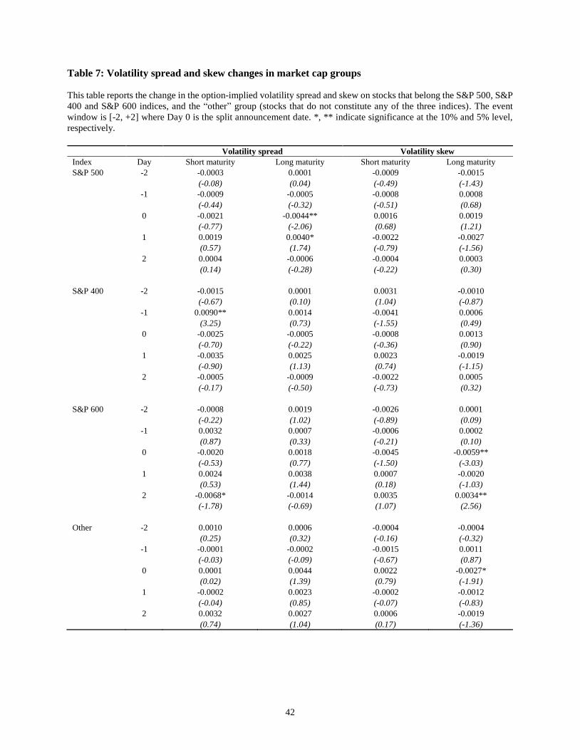
sub-sample analysis for the market cap groups in table 7 broadly corroborates these findings. The

only significant change documented is on day -1 for short maturity options in S&P400 stocks for

the volatility spread7. Prima facie, this significantly positive change implies that option traders

expect positive announcement returns in S&P400 stocks. However, it is not supported by a

7 In the broader [-5, +5] window, there are a few significant changes in spreads and skews in various market cap groups.

They do not affect the inferences reached in this section though.

23

concurrent reduction in the volatility skew. Although the skew does decrease on day -1, it does not

do so significantly (t-stat of -1.55). Further, given that this is the only instance of a significant

change prior to the announcement, we are wary of placing too much emphasis on this result. In

sum, there is little evidence in the pre-announcement spread and skew changes to support the

contention that option investors are trading in anticipation of positive announcement returns.

[Insert Tables 6 and 7 here]

Our earlier analysis of volatility perceptions is indicative of pre-announcement information

leakage. Given this, a possible interpretation of our return perception findings is that the

announcement returns are not large enough to induce option investors to trade. In un-tabulated

results, the mean CAR(0, +1) of our split sample is 2.01% (t-stat is 13.68) and the median is 1.41%.

Further, 68% of our sample had a positive CAR. Although the announcement return is clearly

statistically significant, an average return of 2% may not be deemed large enough given the risk.

Turning our attention to the post-announcement period, table 6 shows that in long maturity

options, there is a weakly significant decrease in the volatility skew on day 0 followed by a

significant decrease on day +1. This decrease in the skew on day +1 is reinforced by a significant

increase in the volatility spread on the same day. These findings suggest that option traders expect

positive longer-term return drift following split announcements. When we look at the market cap

groups in table 7 though, this inference becomes murky. The significant increase in the volatility

spread in long maturity options on day +1 in the full sample appears to be driven by S&P500 stocks.

The spread increase on day +1 is weakly significant for this group and insignificant in the other

three size groups. However, there is a significant decrease in the spread on day 0 in long maturity

options for S&P500 stocks. Given this conflict, one cannot argue that the expectation of positive

return drift in the full sample is driven by S&P500 stocks. For the volatility skew, it is insignificant

on day +1 in long maturity options in all size groups, in contrast to the full sample. There is a

24

significant decrease in the skew on day 0 in long maturity options for the S&P 600 and “other”

group, which conforms with the aggregate results. Thus, if the volatility skew findings point to an

expectation of longer-term return drift, then this drift appears to be driven by smaller stocks.

Overall, we find some evidence that option traders expect positive return drift over the longer-term,

particularly in smaller stocks, but the results are far from conclusive.

4.3 Sensitivity analysis

When splits are announced, it is common for firms to announce other information simultaneously.

As an example, for around 30 percent of our sample, stock splits and cash dividends are

concurrently announced. Given this, we repeat the analysis for firms that do not have a

simultaneous release of other information during the period [-10, +10]. Appendix A presents the

findings. The results are very similar to the analogous output in tables 4 and 6. There is evidence

of an increase in implied volatility in both call and put options prior to Day 0. Once the split is

announced, the increase in implied volatility is stronger and more persistent for options that expire

after the effective date. With regard to the volatility spread and skew, once again, we see a

significantly positive (negative) change in the volatility spread (skew) on Day +1. In unreported

results, we find that this significant change is mainly driven by stocks that belong to the S&P 600

index and the “other” group. In sum, our findings are robust to the simultaneous release of other

information.

The statistical significance of the change in implied volatility, and the volatility spread

(skew) is inferred based on the assumption that the expected daily change in these measures is zero.

To verify this condition, we examine the distribution of these changes during the period [-100, -

20]. Appendix B reports that the daily change in these measures is very small, particularly in

comparison to the changes observed during the event window of [-5, +5]. Nevertheless, to ensure

25

that our analysis is not influenced by cross-sectional variation in the expected change in implied

volatility and the volatility spread (skew), for each firm, we select a benchmark. Specifically, the

expected daily change is proxied using the average change in these measures during the period [-

100, -20]. The abnormal change is then computed by subtracting the appropriate benchmark. The

findings are presented in appendices C and D, which replicate tables 4 and 6 but with abnormal

changes. In short, the behavior of the abnormal change in implied volatility and the volatility spread

(skew) is very similar to the raw change in these metrics.

5. The predictive ability of option measures

In the analysis of option traders’ perceptions on future stock volatility, we document numerous

cases where implied volatility significantly increases in short maturity options prior to the

announcement. We interpret this as evidence that option traders are acquiring and trading on private

information prior to split announcements. We also conjecture that the significant increases

observed are unlikely to be solely due to trading on leaked information and that they also probably

entail a skillful reaction by other informed traders who are responding to the trading activity

observed. However, we cannot isolate to what extent the trading is based on leaked information or

skillful processing of public information. What we can say with a reasonable degree of certainty is

that the implied volatility increases are strongly suggestive of trading on leaked information. To

more directly address whether option traders are skillfully processing information (public or

private), we analyze whether pre-event option trading predicts future changes in the return

distribution of the underlying stocks.

Given that we have already documented informed trading using pre-announcement changes

in implied volatility, we rely on these changes again in our analysis on the predictability of

volatility. Specifically, we run cross-sectional regressions of stock volatility levels at the

26

announcement on changes in implied volatility prior to the announcement. As with all the pre-

announcement analyses, we focus on short maturity options. Our reasons for doing so are similar

to before. If option investors are trading on stock volatility levels in the near future, they are likely

to employ shorter-dated options to do so. Additionally, the significant changes in pre-

announcement implied volatility are observed in short maturity options.

Table 8 shows that implied volatility changes in short maturity options prior to the

announcement do not predict abnormal stock volatility on day 0. However, for stock volatility on

day +1, there are significantly positive coefficients in short maturity options on day -2 in calls and

on days -5, -3, -2 and -1 in puts. This indicates that pre-announcement implied volatility changes

predict stock volatility levels on the day after the announcement. A possible reason for the lack of

predictability on day 0 is noise associated with the announcement. Once this noise mitigates, the

predictability appears on the following day. These predictability findings complement our earlier

results quite nicely. Not only do we document significant increases in implied volatility prior to

the announcement, we also show that implied volatility changes predict stock volatility levels after

the announcement. More broadly, the perceptions analysis highlights option traders’ capacity to

acquire private information. Here we show that they also display an ability to process information

skillfully.

[Insert Table 8]

In the volatility perceptions analysis, when we examined implied volatility changes after

the announcement, we saw significant increases in both long maturity calls and puts on day +1. We

interpreted this as evidence that option traders expect an increase in stock volatility after splits are

effected. Now we consider whether changes in implied volatility after the announcement can

predict the post-split change in stock volatility. Here we are interested in long maturity options.

27

This is because option traders will likely employ longer-dated options that expire after the effective

date if they are trading on post-split stock volatility changes.

Table 9 shows that the coefficients on the change in implied volatility on day +1 in both

long maturity calls and puts are significantly positive. There is also a weakly significant positive

coefficient on day +5 in long maturity puts. These findings indicate that changes in implied

volatility after the announcement predict the post-split change in stock volatility. Again, the

regression findings on the predictability of volatility complement the perceptions analysis well.

Previously, we documented significant increases in implied volatility on day +1 for both long

maturity calls and puts. Now we show that the change in implied volatility for these option groups

on day +1 predicts the change in stock volatility after splits are effected. The private informational

advantage of option traders is likely to be low directly after the announcement. As such, our

interpretation of these findings is that option traders are displaying skill in processing public

information8.

[Insert Table 9]

We now turn our attention to the predictability of future returns. First, we consider the

predictability of the announcement returns. To do so, we run regressions of the CAR(0, +1) on the

pre-announcement level of the volatility spread and skew. There are no significant coefficients on

the spread or skew in Table 10. This implies that the pre-announcement spread and skew do not

predict the announcement returns. In the perceptions analysis, we find little evidence that option

8 In unreported results, we find that the regression output assessing the predictability of volatility is very similar when

we constrain the sample to only include splitters that do not have a simultaneous release of other information. When

we run the regressions on the four market cap groups, we find that the “other” portfolio tends to drive the significant

coefficients reported in tables 8 and 9. The S&P500, S&P400 and S&P600 groups also contribute to the significant

findings but to a lesser extent.

28

investors are trading to exploit the positive announcement returns. We add to this here by

documenting that our option measures do not predict the announcement returns.

[Insert Table 10]

Chan, Ge and Lin (2014) contend that even though the average announcement returns of

acquirers is close zero, there is large variation in these returns across acquirers. They find that the

spread and skew do predict the announcement returns of acquiring firms. With splits, there is much

less dispersion in the announcement returns. As discussed previously, the average (median) CAR

is 2% (1.4%) and 68% of our sample has a positive CAR. Thus, a possible explanation of our

findings is that option traders find it difficult to differentiate between the announcement returns of

splitting firms.

Lastly, we consider whether spread and skew levels after the announcement can predict

future return drift. Here we are assessing option traders’ ability to interpret information in the split

announcement on subsequent return drift. In Table 11, there is a significantly positive coefficient

on the spread in short maturity options on day +1. There is also a weakly significant positive

coefficient on the spread on day +4, again in short maturity options. These findings suggest that

post-announcement option trading predicts return drift in the shorter-term. However, the

significantly positive coefficients on the spread are not supported by significantly negative

coefficients on the skew for the corresponding days. Overall, the evidence on whether post-

announcement spread and skew levels predict future return drift is weak9.

[Insert Table 11]

9 For consistency with our earlier analyses and for completeness, we rerun the regressions on return predictability but

using the daily change in the spread and skew rather than the level. Appendices E and F report the output. There is

little in these results that would suggest that the change in spread and skew can predict either the announcement returns

or longer-term return drift.

29

6. Conclusion

This study investigates informed option trading around stock split announcements. To do so, we

assess the perceptions of option traders on future stock return and volatility changes due to splits.

We also test whether option trading around the event predicts future changes in stock returns and

volatility. By considering both perceptions and predictability, we provide a more comprehensive

picture of informed trading in options.

We find that option trading activity prior to the announcement indicates that option

investors anticipate an increase in stock volatility soon after the announcement. Given that splits

are unscheduled events that the market should not have foreknowledge of, this is suggestive of

information leakage prior to the announcement. Option trading after the announcement implies that

option investors expect stock volatility to increase after splits are effected. There is little evidence

though that option investors are trading in anticipation of positive announcement returns or return

drift in the longer-term. As a whole, the perceptions analysis indicates that option trading around

the event is largely motivated by expected changes in future stock volatility.

Next, we show that pre-event option trading predicts the level of stock volatility soon after

the announcement. This highlights option traders’ capacity to skillfully process information prior

to the announcement. It also complements the perceptions analysis nicely where we show that

option traders demonstrate an ability to acquire information on the impending event. Lastly, we

find that option trading soon after the announcement predicts the change in stock volatility after

splits are effected. Given that informed traders’ private informational advantage is likely to be low

soon after public announcements, we contend that this emphasizes option traders’ skill in

processing public information.

In sum, we show that option traders display a capacity to both acquire and skillfully process

information prior to split announcements. We also show that they are adept at analyzing public

30

information after the announcement. Collectively, we document strong evidence of informed

trading in options around split announcements.

31

References

An, B.J., Ang, A., Bali, T.G., Cakici, N., 2014. The joint cross section of stocks and options. Journal

of Finance 69, 2279-2337.

Anand, A., Chakravarty, S., 2007. Stealth trading in options markets. Journal of Financial and

Quantitative Analysis 42, 167-188.

Atilgan, Y., 2014. Volatility spreads and earnings announcement returns. Journal of Banking and

Finance 38, 205-215.

Black, F., 1975. Fact and fantasy in the use of options. Financial Analysts Journal 31, 36-41, 61-

72.

Bodnaruk, A., Massa, M., Simonov, A., 2009. Investment banks as insiders and the market for

corporate control. Review of Financial Studies 22, 4989-5026.

Boehme, R.D., Danielsen, B.R., 2007. Stock split post-announcement returns: Underreaction or

market friction. Financial Review 42, 485-506.

Bollen, N., Whaley, R., 2004. Does net buying pressure affect the shape of implied volatility

functions? Journal of Finance 59,711–753

Byun, J., Rozeff, M. S., 2003. Long-run performance after stock splits: 1927 to 1996. Journal of

Finance 58, 1063-85.

Chan, K., Ge, L., Lin, T.C., 2014. Informational content of options trading on acquirer

announcement return. Journal of Financial and Quantitative Analysis forthcoming.

Chern, K.H., Tandon, K., Yu, S., Webb, G., 2008. The information content of stock split

announcements: Do options matter? Journal of Banking and Finance 32, 930-946.

Cox, J.C., Ross, S.A., Rubinstein, M., 1979. Option pricing: A simplified approach. Journal of

Financial Economics 7, 229-63.

32

Cremers, M., Weinbaum, D., 2010. Deviations from put-call parity and stock return predictability.

Journal of Financial and Quantitative Analysis 45, 335-67.

Desai, H., Jain, P. C., 1997. Long run common stock returns following stock splits and reverse

splits. Journal of Business 70, 409-33.

Diavatopoulos, D., Doran, J.S., Fodor, A., Peterson, D.R., 2012. The information content of

implied skewness and kurtosis changes prior to earnings announcements for stock and

option returns. Journal of Banking and Finance 36, 786-802.

Doran, J., Peterson, D., Tarrant, B., 2007. Is there information in the volatility skew? Journal of

Futures Markets 27, 921-960.

Dravid, A.R., 1987. A note on the behavior of stock returns around ex-dates of stock distributions.

Journal of Finance 42, 163–168.

Easley, D., O'Hara, M., Srinivas, P. S., 1998. Option volume and stock prices: Evidence on where

informed traders trade. Journal of Finance 53, 431–65.

Engelberg, J.E., Reed, A.V., Ringgenberg, M.C., 2012. How are shorts informed? Short sellers,

news, and information processing. Journal of Financial Economics 105, 250-278.

French, D., Dubofsky, D., 1986. Stock splits and implied stock price volatility. Journal of Portfolio

Management 12, 55-59.

Garleanu, N., Pedersen, L., Poteshman, A., 2009. Demand-based option pricing. Review of

Financial Studies 22, 4259-4299

Grinblatt, M.S., Masulis, R.W., Titman, S., 1984. The valuation effects of stock splits and stock

dividends. Journal of Financial Economics 13, 461-490.

Hayunga, D., Lung, P., 2014. Trading in the option market around the financial analysts’ consensus

revision. Journal of Financial and Quantitative Analysis forthcoming.

33

Ikenberry, D.L., Rankine, G., Stice, E.K., 1996. What do stock splits really signal? Journal of

Financial and Quantitative Analysis 31, 357-75.

Ikenberry, D.L., Ramnath, S., 2002. Underreaction to self-selected news events: The case of stock

splits. Review of Financial Studies 15, 489-526.

Ivashina, V., Sun, Z., 2011. Institutional stock trading and loan market information. Journal of


Jin, W., Livnat, J., Zhang, Y., 2012. Option prices leading equity prices: Do option traders have an

information advantage? Journal of Accounting Research 50, 401-432.

Johnson, T.L., So, E.C., 2012. The option to stock volume ratio and future returns. Journal of


Karpoff, J.M., Lou, X., 2010. Short sellers and financial misconduct. Journal of Finance 65, 1879-

1913.

Koski, J., 1998. Measurement effects and the variance of returns after stock splits and stock

dividends. Review of Financial Studies 11, 143-162.

Lin, J.C., Singh, A.K., Yu, W., 2009. Stock splits, trading continuity, and the cost of equity capital.

Journal of Financial Economics 93, 474-489.

Lung, P.P., Xu, P., 2014. Tipping and option trading. Financial Management 43, 671-701.

Massoud, N., Nandy, D., Saunders, A., Song, K., 2011. Do hedge funds trade on private

information? Evidence from syndicated lending and short-selling. Journal of Financial

Economics 99, 477-499.

Ohlson, J., Penman, S., 1985. Volatility increases subsequent to stock splits: An empirical

aberration. Journal of Financial Economics 14, 251-66.

Reilly, F.K., Gustavson, S.G., 1985. Investing in options on stocks announcing splits. Financial

Review 20, 121–142.

34

Roll, R., Schwartz, E., Subrahmanyam, A., 2010. O/S: The relative trading activity in options and

stocks. Journal of Financial Economics 96, 1-17.

Sheikh, A.M., 1989. Stock splits, volatility increases, and implied volatilities. Journal of Finance

44, 1361-1372.

Xing, Y., Zhang, X., Zhao, R., 2010. What does the individual option volatility smirk tell us about

future equity returns? Journal of Financial and Quantitative Analysis 45, 641-662.

35

Appendix 1: Description of the control variables

The CAR regressions (equations (9) and (10)) and the BHAR regressions (equations (11) and (12))

employ the following control variables:

Size: is the natural logarithm of the firm’s market capitalization at the end of the month prior to the

announcement date.

Analyst: is the number of analysts following the firm for the earnings quarter before the

announcement date.

Book-to-market ratio: is the firm’s book value of equity at the end of the fiscal year preceding the

calendar year of the announcement date divided by the firm’s market capitalization at the end of

the month prior to the announcement date.

Price: is the natural logarithm of the stock’s price 20 days prior to the announcement date.

Volume: is the average dollar trading volume of the stock during the period [-250, -11].

Run-up: is the BHAR [-250, -11].

Arbitrage risk: is the standard deviation of the residuals from a market model regression using the

past 48 months of stock returns.

Market risk: is the R-square of the regression used to estimate arbitrage risk.

Split factor.

In addition, the BHAR (+7, +60) regressions also include the CAR (0, +1) as a control variable.

36

Table 1: Summary statistics on option liquidity and implied volatility

This table reports the liquidity and implied volatility for both call and put options at different levels of moneyness for

the 10 day period [-60 to -50] where Day 0 is the split announcement date. The option’s degree of moneyness is

measured using option delta, which is the risk-neutral probability of the option being in-the-money at expiration. Panel

A reports the mean/median volume (Vol), open interest (OI) and implied volatility (IV) for call options while panel B

reports the same information for put options. The sample period is 1998-2012.

Panel A: Call options

Moneyness index Option delta Mean OI Median OI Mean Vol Median Vol Mean IV

Deep out-of-the-money 0.02<delta<=0.125 1480 287 91 2 0.5521

Out-of-the-money 0.125<delta<=0.375 940 151 114 5 0.5240

Near-the-money 0.375<delta<=0.625 825 139 117 7 0.5538

In-the-money 0.625<delta<=0.875 649 89 50 0 0.5601

Deep in-the-money 0.875<delta<=0.98 444 45 13 0 0.6462

Panel B: Put options

Moneyness index Option delta Mean OI Median OI Mean Vol Median Vol Mean IV

Deep out-of-the-money -0.125<delta<=-0.02 1068 201 49 0 0.6716

Out-of-the-money -0.375<delta<=-0.125 676 80 71 0 0.5853

Near-the-money -0.625<delta<=-0.375 380 25 50 0 0.5682

In-the-money -0.875<delta<=-0.625 213 6 17 0 0.5341

Deep in-the-money -0.98<delta<=-0.875 161 0 6 0 0.5840

37

Table 2: Summary statistics for market cap groups

This table reports the liquidity and implied volatility for call and put options on stocks that belong to the S&P 500

(large cap stocks), S&P 400 (mid cap stocks) and S&P 600 indices (small cap stocks), and “other” stocks (stocks that

are not part of any of these three indices). Panel A reports the mean/median volume (Vol), open interest (OI), and the

average implied volatility (IV) for call options during the period [-60 to -50] where Day 0 is the split announcement

date. Panel B reports the same information for put options.


Index Option delta Mean OI Median OI Mean Vol Median Vol Mean IV

S&P 500 0.02<delta<=0.125 2625 638 151 12 0.3940

0.125<delta<=0.375 2179 557 261 29 0.3802

0.375<delta<=0.625 2077 594 293 34 0.3982

0.625<delta<=0.875 1616 359 124 5 0.4149

0.875<delta<=0.98 1001 165 29 0 0.5289

S&P400 0.02<delta<=0.125 801 264 56 0 0.5127

0.125<delta<=0.375 532 134 61 2 0.4811

0.375<delta<=0.625 522 142 70 5 0.5019

0.625<delta<=0.875 403 88 25 0 0.5000

0.875<delta<=0.98 222 30 6 0 0.6117

S&P 600 0.02<delta<=0.125 197 74 14 0 0.5972

0.125<delta<=0.375 226 50 24 0 0.5115

0.375<delta<=0.625 219 53 25 0 0.5140

0.625<delta<=0.875 167 35 11 0 0.5206

0.875<delta<=0.98 106 12 3 0 0.6209

Other 0.02<delta<=0.125 629 166 50 0 0.7787

0.125<delta<=0.375 401 95 57 1 0.6962

0.375<delta<=0.625 371 88 60 5 0.7140

0.625<delta<=0.875 300 56 27 0 0.7249

0.875<delta<=0.98 230 36 9 0 0.8054


Index Option delta Mean OI Median OI Mean Vol Median Vol Mean IV

S&P 500 -0.125<delta<=-0.02 2219 751 93 3 0.5094

-0.375<delta<=-0.125 1691 455 167 13 0.4247

-0.625<delta<=-0.375 995 169 130 6 0.4075

-0.875<delta<=-0.625 517 48 43 0 0.4010

-0.98<delta<=-0.875 360 10 13 0 0.4455

S&P400 -0.125<delta<=-0.02 525 134 22 0 0.6101

-0.375<delta<=-0.125 399 78 43 0 0.5247

-0.625<delta<=-0.375 223 24 29 0 0.5109

-0.875<delta<=-0.625 110 4 9 0 0.4794

-0.98<delta<=-0.875 54 0 4 0 0.5281

S&P 600 -0.125<delta<=-0.02 288 59 12 0 0.6391

-0.375<delta<=-0.125 168 30 18 0 0.5458

-0.625<delta<=-0.375 94 10 10 0 0.5212

-0.875<delta<=-0.625 60 0 4 0 0.5001

-0.98<delta<=-0.875 22 0 1 0 0.6178

Other -0.125<delta<=-0.02 397 105 27 0 0.8678

-0.375<delta<=-0.125 271 42 37 0 0.7611

-0.625<delta<=-0.375 156 11 23 0 0.7358

-0.875<delta<=-0.625 102 1 8 0 0.7066

-0.98<delta<=-0.875 85 0 3 0 0.7883

38

Table 3: Summary statistics on the volatility spread and skew

This table reports the distribution of the volatility spread and skew for the period [-60 to -50] where Day 0 is the split

announcement date. Panel A reports the summary statistics for the full sample while Panel B reports the same

information for each market capitalization group. The volatility spread is the weighted average of the difference in

implied volatility across all valid call and put option pairs matched on the same strike price and maturity date. The

weight is the average open interest of the call and put options. The volatility skew is the difference in implied volatility

of out-of-the-money put and at-the-money call options. Out-of-the-money put options are those with delta closest to -

0.3 and at-the-money call options are those with delta closest to 0.5.

Panel A: Full sample

Volatility spread Volatility skew

Mean -0.0174 0.0318

25th percentile -0.0294 0.0024

Median -0.0089 0.0214

75th percentile 0.0035 0.0440

Standard deviation 0.0556 0.0415

Panel B: Market capitalization groups

Index Volatility spread Volatility skew

S&P 500 Mean -0.0084 0.0239


Median -0.0054 0.0184



S&P 400 Mean -0.0097 0.0293


Median -0.0059 0.0215



S&P 600 Mean -0.0132 0.0327


Median -0.0073 0.0226



Other Mean -0.0258 0.0398


Median -0.0165 0.0265



39

Table 4: Implied volatility changes around split announcements

This table reports the change in implied volatility for call and put options around the split announcement date. The

event window is [-5, +5] where Day 0 is the announcement date. Short maturity options expire before the effective

date while long maturity options expire after the effective date. The sample period is 1998-2012. Numbers in

parentheses are the t-statistic of the means. *,** indicate significance at the 10% and 5% level, respectively.

Call Put

Day Short maturity Long maturity Short maturity Long maturity

-5 0.0035* 0.0014 0.0021 0.0012*

(1.75) (1.20) (1.62) (1.75)

-4 -0.0002 -0.0002 0.0023* 0.0008

(-0.08) (-0.17) (1.70) (1.03)

-3 0.0067** -0.0012 0.0019 -0.0013**

(3.08) (-1.08) (1.37) (-2.01)

-2 0.0089** 0.0025** 0.0050** 0.0020**

(3.57) (2.69) (3.52) (3.00)

-1 0.0084** 0.0015 0.0067** -0.0004

(3.54) (1.48) (4.07) (-0.61)

0 0.0124** 0.0117** 0.0156** 0.0118**

(4.51) (7.87) (7.98) (11.74)

1 -0.0025 0.0064** -0.0056** 0.0026**

(-0.94) (4.57) (-2.50) (2.41)

2 0.0030 -0.0004 0.0015 -0.0003

(1.04) (-0.34) (0.70) (-0.40)

3 0.0049 0.0000 0.0023 0.0012

(1.63) (0.04) (1.31) (1.63)

4 0.0014 -0.0009 0.0026 -0.0001

(0.56) (-0.91) (1.47) (-0.14)

5 0.0010 -0.0001 0.0016 0.0007

(0.35) (-0.14) (0.83) (1.04)

40

Table 5: Implied volatility changes in market cap groups

This table reports the change in implied volatility for call and put options on stocks that belong to the S&P 500, S&P

400 and S&P 600 indices, and the “other” group (stocks that do not constitute any of the three indices). The event

window is [-2, +2] where Day 0 is the split announcement date. *, ** indicate significance at the 10% and 5% level,

respectively.

Call Put

Index Day Short maturity Long maturity Short maturity Long maturity

S&P 500 -2 0.0068* 0.0009 0.0056** 0.0029*

(1.91) (0.52) (2.66) (1.89)

-1 0.0012 0.0017 0.0049** -0.0013

(0.37) (1.14) (2.48) (-0.96)

0 0.0084** 0.0051** 0.0138** 0.0115**

(2.39) (2.18) (3.70) (6.68)

1 -0.0058 0.0031 -0.0113** -0.0018

(-1.36) (1.37) (-3.04) (-1.08)

2 0.0016 -0.0005 -0.0004 -0.0019

(0.34) (-0.24) (-0.13) (-1.12)

S&P 400 -2 0.0021 0.0018 0.0053** 0.0011

(0.50) (1.04) (2.27) (0.96)

-1 0.0094** 0.0020 0.0012 -0.0005

(2.07) (0.82) (0.45) (-0.45)

0 0.0108** 0.0122** 0.0151** 0.0106**

(2.66) (3.75) (3.98) (6.22)

1 -0.0006 0.0028 -0.0011 0.0022

(-0.11) (1.05) (-0.36) (1.35)

2 -0.0031 -0.0014 0.0019 0.0003

(-0.79) (-0.63) (0.43) (0.24)

S&P 600 -2 0.0145** 0.0036* 0.0020 0.0010

(2.80) (1.80) (0.58) (0.77)

-1 0.0051 0.0007 0.0095** -0.0003

(1.00) (0.34) (2.68) (-0.22)

0 0.0142** 0.0131** 0.0137** 0.0093**

(2.54) (4.60) (3.19) (4.48)

1 0.0043 0.0075** -0.0010 0.0021

(0.76) (3.14) (-0.20) (1.23)

2 0.0014 0.0003 0.0084* 0.0043**

(0.20) (0.13) (1.87) (3.14)

Other -2 0.0116* 0.0034* 0.0066** 0.0029**

(1.94) (1.77) (2.06) (2.10)

-1 0.0164** 0.0017 0.0102** 0.0002

(2.99) (0.85) (2.52) (0.15)

0 0.0159** 0.0151** 0.0189** 0.0146**

(2.25) (4.88) (5.00) (6.79)

1 -0.0057 0.0104** -0.0070 0.0062**

(-1.04) (3.25) (-1.34) (2.40)

2 0.0099 -0.0002 -0.0024 -0.0031*

(1.58) (-0.09) (-0.52) (-1.79)

41

Table 6: Volatility spread and skew changes around split announcements

This table reports the change in the option-implied volatility spread and skew. The volatility spread is calculated as the

weighted average difference in implied volatility between call and put options matched on the same strike price and

maturity date. The weight is the average open interest of the call and put options. The volatility skew is the difference

in implied volatility between out-of-the-money put options and at-the-money call options. An out-of-the-money put

option is one whose delta is closest to -0.3 and an at-the-money call option is one whose delta is closest to 0.5. The

event window is [-5, +5] where Day 0 is the announcement date. *, ** indicate significance at the 10% and 5% level,

respectively.



-5 0.0007 0.0023* -0.0003 -0.0007

(0.46) (1.83) (-0.26) (-0.90)

-4 -0.0004 -0.0012 -0.0020 -0.0005

(-0.25) (-1.22) (-1.57) (-0.83)

-3 0.0002 -0.0003 0.0013 0.0001

(0.14) (-0.35) (1.18) (0.11)

-2 -0.0003 0.0007 -0.0003 -0.0007

(-0.16) (0.71) (-0.21) (-1.04)

-1 0.0023 0.0003 -0.0016 0.0007

(1.49) (0.28) (-1.44) (1.07)

0 -0.0015 0.0007 0.0002 -0.0014*

(-0.78) (0.50) (0.18) (-1.71)

1 0.0002 0.0031** -0.0002 -0.0019**

(0.11) (2.41) (-0.13) (-2.27)

2 -0.0004 0.0002 0.0002 0.0003

(-0.19) (0.18) (0.14) (0.40)

3 -0.0007 -0.0011 0.0010 0.0004

(-0.40) (-1.03) (0.86) (0.66)

4 0.0002 -0.0007 -0.0011 0.0004

(0.11) (-0.72) (-0.84) (0.70)

5 -0.0035** -0.0013 -0.0012 0.0009

(-2.05) (-1.29) (-1.09) (1.35)

42

Table 7: Volatility spread and skew changes in market cap groups

This table reports the change in the option-implied volatility spread and skew on stocks that belong the S&P 500, S&P

400 and S&P 600 indices, and the “other” group (stocks that do not constitute any of the three indices). The event

window is [-2, +2] where Day 0 is the split announcement date. *, ** indicate significance at the 10% and 5% level,

respectively.


Index Day Short maturity Long maturity Short maturity Long maturity

S&P 500 -2 -0.0003 0.0001 -0.0009 -0.0015

(-0.08) (0.04) (-0.49) (-1.43)

-1 -0.0009 -0.0005 -0.0008 0.0008

(-0.44) (-0.32) (-0.51) (0.68)

0 -0.0021 -0.0044** 0.0016 0.0019

(-0.77) (-2.06) (0.68) (1.21)

1 0.0019 0.0040* -0.0022 -0.0027

(0.57) (1.74) (-0.79) (-1.56)

2 0.0004 -0.0006 -0.0004 0.0003

(0.14) (-0.28) (-0.22) (0.30)

S&P 400 -2 -0.0015 0.0001 0.0031 -0.0010

(-0.67) (0.10) (1.04) (-0.87)

-1 0.0090** 0.0014 -0.0041 0.0006

(3.25) (0.73) (-1.55) (0.49)

0 -0.0025 -0.0005 -0.0008 0.0013

(-0.70) (-0.22) (-0.36) (0.90)

1 -0.0035 0.0025 0.0023 -0.0019

(-0.90) (1.13) (0.74) (-1.15)

2 -0.0005 -0.0009 -0.0022 0.0005

(-0.17) (-0.50) (-0.73) (0.32)

S&P 600 -2 -0.0008 0.0019 -0.0026 0.0001

(-0.22) (1.02) (-0.89) (0.09)

-1 0.0032 0.0007 -0.0006 0.0002

(0.87) (0.33) (-0.21) (0.10)

0 -0.0020 0.0018 -0.0045 -0.0059**

(-0.53) (0.77) (-1.50) (-3.03)

1 0.0024 0.0038 0.0007 -0.0020

(0.53) (1.44) (0.18) (-1.03)

2 -0.0068* -0.0014 0.0035 0.0034**

(-1.78) (-0.69) (1.07) (2.56)

Other -2 0.0010 0.0006 -0.0004 -0.0004

(0.25) (0.32) (-0.16) (-0.32)

-1 -0.0001 -0.0002 -0.0015 0.0011

(-0.03) (-0.09) (-0.67) (0.87)

0 0.0001 0.0044 0.0022 -0.0027*

(0.02) (1.39) (0.79) (-1.91)

1 -0.0002 0.0023 -0.0002 -0.0012

(-0.04) (0.85) (-0.07) (-0.83)

2 0.0032 0.0027 0.0006 -0.0019

(0.74) (1.04) (0.17) (-1.36)

43

Table 8: Regressions of announcement volatility on changes in implied volatility

This table reports the output from the cross-sectional regressions of abnormal daily stock volatility (AbVol) on the

change in option-implied volatility (∆IV) for the sample of splitting firms. Abnormal daily stock volatility is estimated

as the square of the daily returns on Day 0 (Day +1) minus the average squared returns over the [-60, -20] period. ∆IV

is defined as in equations (1) and (2). Panel A reports the coefficients on ∆IV and the associated t-statistics for call

options while panel B reports the same information for put options. Intercepts have been suppressed to conserve space.

Short maturity options expire before the effective date while long maturity options expire after the effective date. The

sample period is 1998-2012. *,** indicate significance at the 10% and 5% level, respectively.


Short maturity Long maturity

Day Day 0 AbVol Day 1 AbVol Day 0 AbVol Day 1 AbVol

-5 0.0012 -0.0058 0.0237 0.0004

(0.41) (-0.88) (1.38) (0.04)

-4 0.0027 -0.0002 0.0037 -0.0067

(1.43) (-0.03) (0.47) (-0.41)

-3 0.0035 -0.0009 0.0082 0.0079

(1.52) (-0.17) (0.96) (1.12)

-2 -0.0016 0.0103** 0.0295 0.0241**

(-0.69) (2.44) (1.10) (2.51)

-1 0.0029 0.0077 0.0111 0.0053

(1.37) (1.24) (0.63) (0.82)


Short maturity Long maturity

Day Day 0 AbVol Day 1 AbVol Day 0 AbVol Day 1 AbVol

-5 0.0171 0.0209** 0.0270* 0.0472

(1.35) (2.11) (1.70) (1.33)

-4 0.0071 -0.0136 0.0347 -0.0193

(1.61) (-1.04) (1.22) (-0.53)

-3 0.0043 0.0179** 0.0078 0.0312

(0.97) (2.43) (0.43) (1.49)

-2 0.0137 0.0223** 0.0359 0.0202

(1.21) (2.57) (1.35) (1.29)

-1 0.0520 0.0228** 0.0463 0.0204

(1.33) (2.11) (0.78) (1.07)

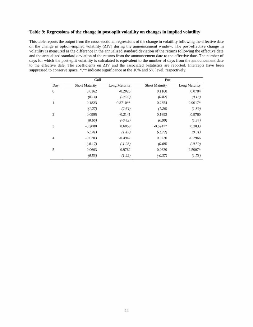
44

Table 9: Regressions of the change in post-split volatility on changes in implied volatility

This table reports the output from the cross-sectional regressions of the change in volatility following the effective date

on the change in option-implied volatility (∆IV) during the announcement window. The post-effective change in

volatility is measured as the difference in the annualized standard deviation of the returns following the effective date

and the annualized standard deviation of the returns from the announcement date to the effective date. The number of

days for which the post-split volatility is calculated is equivalent to the number of days from the announcement date

to the effective date. The coefficients on ∆IV and the associated t-statistics are reported. Intercepts have been

suppressed to conserve space. *,** indicate significance at the 10% and 5% level, respectively.

Call Put

Day Short Maturity Long Maturity Short Maturity Long Maturity

0 0.0162 -0.2025 0.1168 0.0784

(0.14) (-0.92) (0.82) (0.18)

1 0.1823 0.8710** 0.2354 0.9017*

(1.27) (2.64) (1.26) (1.89)

2 0.0995 -0.2141 0.1693 0.9760

(0.65) (-0.42) (0.90) (1.34)

3 -0.2080 0.6059 -0.5247* 0.3033

(-1.41) (1.47) (-1.72) (0.31)

4 -0.0203 -0.4942 0.0230 -0.2966

(-0.17) (-1.23) (0.08) (-0.50)

5 0.0603 0.9762 -0.0629 2.5907*

(0.53) (1.22) (-0.37) (1.73)

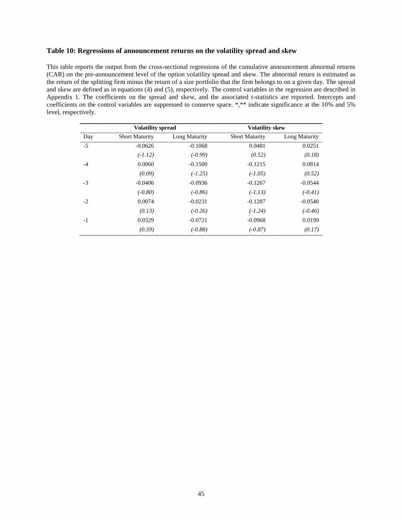
45

Table 10: Regressions of announcement returns on the volatility spread and skew

This table reports the output from the cross-sectional regressions of the cumulative announcement abnormal returns

(CAR) on the pre-announcement level of the option volatility spread and skew. The abnormal return is estimated as

the return of the splitting firm minus the return of a size portfolio that the firm belongs to on a given day. The spread

and skew are defined as in equations (4) and (5), respectively. The control variables in the regression are described in

Appendix 1. The coefficients on the spread and skew, and the associated t-statistics are reported. Intercepts and

coefficients on the control variables are suppressed to conserve space. *,** indicate significance at the 10% and 5%

level, respectively.



-5 -0.0626 -0.1068 0.0481 0.0251

(-1.12) (-0.99) (0.52) (0.18)

-4 0.0060 -0.1500 -0.1215 0.0814

(0.09) (-1.25) (-1.05) (0.52)

-3 -0.0406 -0.0936 -0.1267 -0.0544

(-0.80) (-0.86) (-1.13) (-0.41)

-2 0.0074 -0.0231 -0.1287 -0.0540

(0.13) (-0.26) (-1.24) (-0.46)

-1 0.0329 -0.0721 -0.0968 0.0199

(0.59) (-0.88) (-0.87) (0.17)

46

Table 11: Regressions of post-announcement returns on the volatility spread and skew

This table reports the output from the cross-sectional regressions of the buy and hold abnormal returns (BHAR) on the

level of the option volatility spread and skew. The BHAR is estimated during the period [+7, +60] as the return of the

splitting firm minus the return of a size portfolio that the firm belongs to on the announcement date. The control

variables in the regression are described in Appendix 1. The coefficients on the spread and skew, and the associated t-

statistics are reported. Intercepts and coefficients on the control variables are suppressed to conserve space. *,**

indicate significance at the 10% and 5% level, respectively.



0 0.2242 0.2996 -0.1959 0.1138

(1.07) (1.32) (-0.46) (0.23)

1 0.5218** 0.4424 -0.4219 -0.3162

(2.05) (1.54) (-1.27) (-0.74)

2 -0.0158 0.0418 -0.2536 -0.1058

(-0.07) (0.14) (-0.69) (-0.20)

3 0.1886 -0.0335 -0.0967 -0.0500

(0.89) (-0.10) (-0.33) (-0.10)

4 0.3996* 0.4536 -0.2773 -0.3166

(1.79) (1.43) (-0.70) (-0.68)

5 -0.2008 -0.0598 0.5075 -0.3286

(-0.85) (-0.20) (1.24) (-0.81)

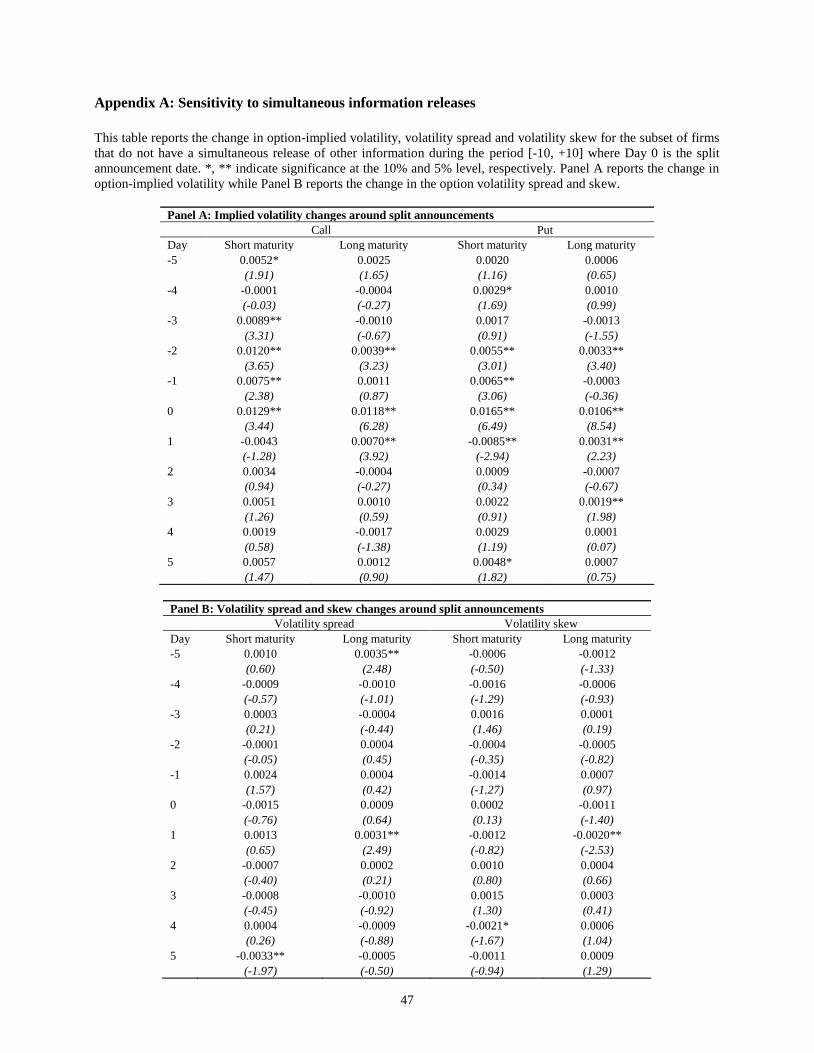
47

Appendix A: Sensitivity to simultaneous information releases

This table reports the change in option-implied volatility, volatility spread and volatility skew for the subset of firms

that do not have a simultaneous release of other information during the period [-10, +10] where Day 0 is the split

announcement date. *, ** indicate significance at the 10% and 5% level, respectively. Panel A reports the change in

option-implied volatility while Panel B reports the change in the option volatility spread and skew.

Panel A: Implied volatility changes around split announcements

Call Put


-5 0.0052* 0.0025 0.0020 0.0006

(1.91) (1.65) (1.16) (0.65)

-4 -0.0001 -0.0004 0.0029* 0.0010

(-0.03) (-0.27) (1.69) (0.99)

-3 0.0089** -0.0010 0.0017 -0.0013

(3.31) (-0.67) (0.91) (-1.55)

-2 0.0120** 0.0039** 0.0055** 0.0033**

(3.65) (3.23) (3.01) (3.40)

-1 0.0075** 0.0011 0.0065** -0.0003

(2.38) (0.87) (3.06) (-0.36)

0 0.0129** 0.0118** 0.0165** 0.0106**

(3.44) (6.28) (6.49) (8.54)

1 -0.0043 0.0070** -0.0085** 0.0031**

(-1.28) (3.92) (-2.94) (2.23)

2 0.0034 -0.0004 0.0009 -0.0007

(0.94) (-0.27) (0.34) (-0.67)

3 0.0051 0.0010 0.0022 0.0019**

(1.26) (0.59) (0.91) (1.98)

4 0.0019 -0.0017 0.0029 0.0001

(0.58) (-1.38) (1.19) (0.07)

5 0.0057 0.0012 0.0048* 0.0007

(1.47) (0.90) (1.82) (0.75)

Panel B: Volatility spread and skew changes around split announcements



-5 0.0010 0.0035** -0.0006 -0.0012

(0.60) (2.48) (-0.50) (-1.33)

-4 -0.0009 -0.0010 -0.0016 -0.0006

(-0.57) (-1.01) (-1.29) (-0.93)

-3 0.0003 -0.0004 0.0016 0.0001

(0.21) (-0.44) (1.46) (0.19)

-2 -0.0001 0.0004 -0.0004 -0.0005

(-0.05) (0.45) (-0.35) (-0.82)

-1 0.0024 0.0004 -0.0014 0.0007

(1.57) (0.42) (-1.27) (0.97)

0 -0.0015 0.0009 0.0002 -0.0011

(-0.76) (0.64) (0.13) (-1.40)

1 0.0013 0.0031** -0.0012 -0.0020**

(0.65) (2.49) (-0.82) (-2.53)

2 -0.0007 0.0002 0.0010 0.0004

(-0.40) (0.21) (0.80) (0.66)

3 -0.0008 -0.0010 0.0015 0.0003

(-0.45) (-0.92) (1.30) (0.41)

4 0.0004 -0.0009 -0.0021* 0.0006

(0.26) (-0.88) (-1.67) (1.04)

5 -0.0033** -0.0005 -0.0011 0.0009

(-1.97) (-0.50) (-0.94) (1.29)

48

Appendix B: Summary statistics for the change in implied volatility, volatility spread and volatility

skew

This table reports the mean, median, standard deviation, skewness and kurtosis of the change in option-implied

volatility, volatility spread and volatility skew during the period [-100, -20] where Day 0 is the split announcement

date. Numbers in parentheses are the t-statistic of the means.

∆IV Call ∆IV Put ∆VS ∆SKEW

Mean -0.000036 -0.000060 -0.000016 -0.000041

(-0.24) (-0.57) (-0.11) (-0.35)

Median -0.000330 -0.000311 0.000046 0.000032

Standard Deviation 0.054 0.038 0.051 0.038

Skewness -0.086 0.810 0.066 0.811

Kurtosis 64 102 128 146

Appendix C: Abnormal change in implied volatility around split announcements

This table reports the abnormal change in implied volatility for call and put options around the split announcement

date. The abnormal change in implied volatility is the change in implied volatility during the event window less the

expected change in implied volatility. The expected change in implied volatility is estimated using the average change

in implied volatility during the period [-100, -20] where Day 0 is the announcement date. Short maturity options expire

before the effective date while long maturity options expire after the effective date. The sample period is 1998-2012.

Numbers in parentheses are the t-statistic of the means. *,** indicate significance at the 10% and 5% level, respectively.

Call Put


-5 0.0037* 0.0016 0.0019 0.0009

(1.79) (1.31) (1.46) (1.34)

-4 -0.0003 -0.0001 0.0025* 0.0012

(-0.16) (-0.10) (1.83) (1.60)

-3 0.0069** -0.0008 0.0020 -0.0010

(3.14) (-0.71) (1.43) (-1.51)

-2 0.0090** 0.0027** 0.0052** 0.0023**

(3.55) (2.76) (3.65) (3.34)

-1 0.0081** 0.0018* 0.0062** -0.0004

(3.38) (1.69) (3.79) (-0.60)

0 0.0124** 0.0115** 0.0152** 0.0116**

(4.42) (7.53) (7.76) (11.41)

1 -0.0016 0.0065** -0.0056** 0.0025**

(-0.61) (4.58) (-2.49) (2.35)

2 0.0032 -0.0005 0.0016 -0.0003

(1.10) (-0.40) (0.78) (-0.37)

3 0.0041 0.0001 0.0023 0.0014*

(1.40) (0.10) (1.28) (1.88)

4 0.0011 -0.0009 0.0031* 0.0001

(0.45) (-0.86) (1.68) (0.13)

5 0.0020 0.0004 0.0016 0.0006

(0.69) (0.35) (0.81) (0.95)

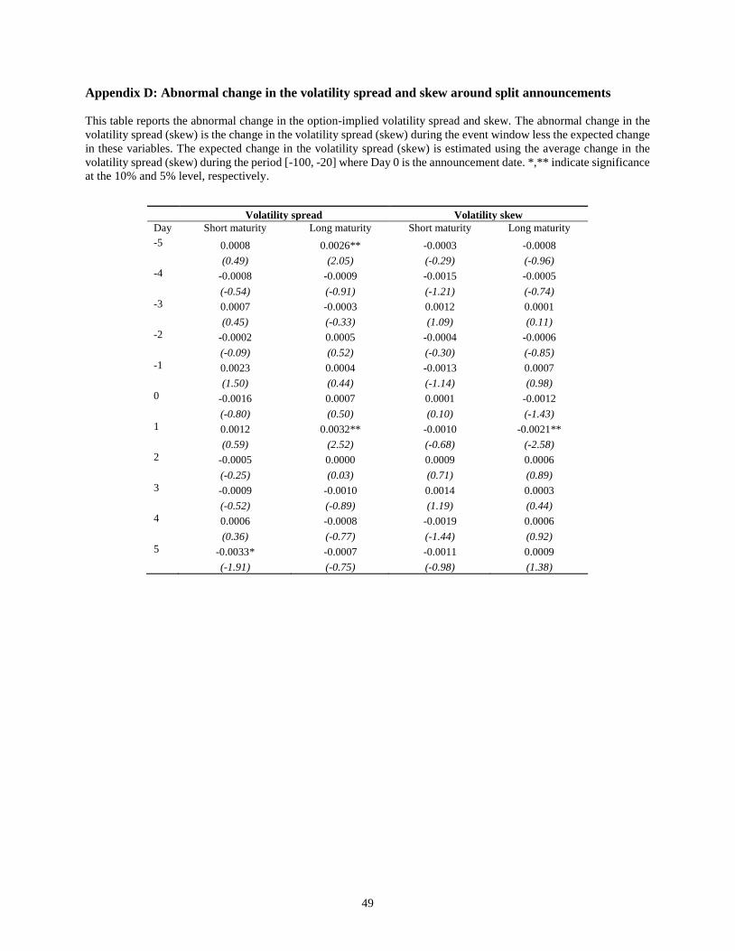
49

Appendix D: Abnormal change in the volatility spread and skew around split announcements

This table reports the abnormal change in the option-implied volatility spread and skew. The abnormal change in the

volatility spread (skew) is the change in the volatility spread (skew) during the event window less the expected change

in these variables. The expected change in the volatility spread (skew) is estimated using the average change in the

volatility spread (skew) during the period [-100, -20] where Day 0 is the announcement date. *,** indicate significance

at the 10% and 5% level, respectively.



-5 0.0008 0.0026** -0.0003 -0.0008

(0.49) (2.05) (-0.29) (-0.96)

-4 -0.0008 -0.0009 -0.0015 -0.0005

(-0.54) (-0.91) (-1.21) (-0.74)

-3 0.0007 -0.0003 0.0012 0.0001

(0.45) (-0.33) (1.09) (0.11)

-2 -0.0002 0.0005 -0.0004 -0.0006

(-0.09) (0.52) (-0.30) (-0.85)

-1 0.0023 0.0004 -0.0013 0.0007

(1.50) (0.44) (-1.14) (0.98)

0 -0.0016 0.0007 0.0001 -0.0012

(-0.80) (0.50) (0.10) (-1.43)

1 0.0012 0.0032** -0.0010 -0.0021**

(0.59) (2.52) (-0.68) (-2.58)

2 -0.0005 0.0000 0.0009 0.0006

(-0.25) (0.03) (0.71) (0.89)

3 -0.0009 -0.0010 0.0014 0.0003

(-0.52) (-0.89) (1.19) (0.44)

4 0.0006 -0.0008 -0.0019 0.0006

(0.36) (-0.77) (-1.44) (0.92)

5 -0.0033* -0.0007 -0.0011 0.0009

(-1.91) (-0.75) (-0.98) (1.38)

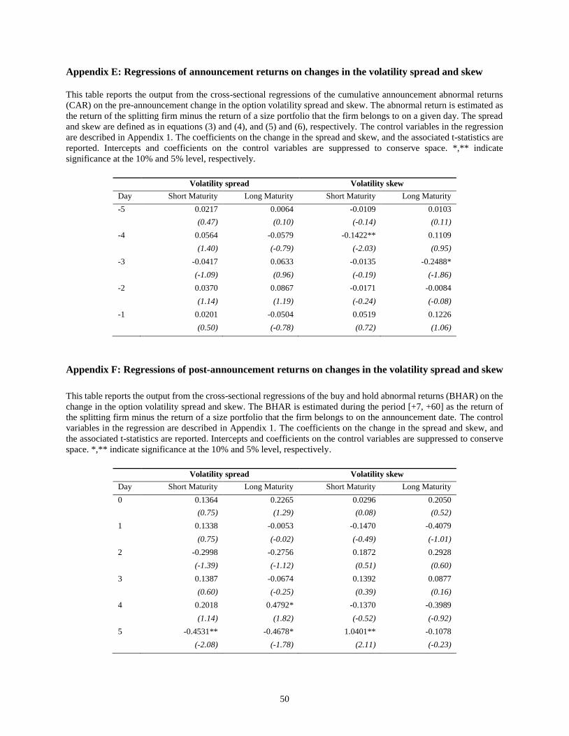
50

Appendix E: Regressions of announcement returns on changes in the volatility spread and skew

This table reports the output from the cross-sectional regressions of the cumulative announcement abnormal returns

(CAR) on the pre-announcement change in the option volatility spread and skew. The abnormal return is estimated as

the return of the splitting firm minus the return of a size portfolio that the firm belongs to on a given day. The spread

and skew are defined as in equations (3) and (4), and (5) and (6), respectively. The control variables in the regression

are described in Appendix 1. The coefficients on the change in the spread and skew, and the associated t-statistics are

reported. Intercepts and coefficients on the control variables are suppressed to conserve space. *,** indicate

significance at the 10% and 5% level, respectively.



-5 0.0217 0.0064 -0.0109 0.0103

(0.47) (0.10) (-0.14) (0.11)

-4 0.0564 -0.0579 -0.1422** 0.1109

(1.40) (-0.79) (-2.03) (0.95)

-3 -0.0417 0.0633 -0.0135 -0.2488*

(-1.09) (0.96) (-0.19) (-1.86)

-2 0.0370 0.0867 -0.0171 -0.0084

(1.14) (1.19) (-0.24) (-0.08)

-1 0.0201 -0.0504 0.0519 0.1226

(0.50) (-0.78) (0.72) (1.06)

Appendix F: Regressions of post-announcement returns on changes in the volatility spread and skew

This table reports the output from the cross-sectional regressions of the buy and hold abnormal returns (BHAR) on the

change in the option volatility spread and skew. The BHAR is estimated during the period [+7, +60] as the return of

the splitting firm minus the return of a size portfolio that the firm belongs to on the announcement date. The control

variables in the regression are described in Appendix 1. The coefficients on the change in the spread and skew, and

the associated t-statistics are reported. Intercepts and coefficients on the control variables are suppressed to conserve

space. *,** indicate significance at the 10% and 5% level, respectively.



0 0.1364 0.2265 0.0296 0.2050

(0.75) (1.29) (0.08) (0.52)

1 0.1338 -0.0053 -0.1470 -0.4079

(0.75) (-0.02) (-0.49) (-1.01)

2 -0.2998 -0.2756 0.1872 0.2928

(-1.39) (-1.12) (0.51) (0.60)

3 0.1387 -0.0674 0.1392 0.0877

(0.60) (-0.25) (0.39) (0.16)

4 0.2018 0.4792* -0.1370 -0.3989

(1.14) (1.82) (-0.52) (-0.92)

5 -0.4531** -0.4678* 1.0401** -0.1078

(-2.08) (-1.78) (2.11) (-0.23)

informed trading around stock split announcements ... annual meetings/2015-amsterdam...informed...

Documents