tabu assisted guided local search approaches for freight service network design

Information Sciences 189 (2012) 266–281

Contents lists available at SciVerse ScienceDirect

Information Sciences

journal homepage: www.elsevier .com/locate / ins

Tabu assisted guided local search approaches for freight servicenetwork design

Ruibin Bai a,⇑, Graham Kendall b, Rong Qu b, Jason A.D. Atkin b

a Division of Computer Science, University of Nottingham Ningbo, Chinab School of Computer Science, University of Nottingham, Nottingham, UK

a r t i c l e i n f o a b s t r a c t

Article history:Received 16 November 2010Received in revised form 12 October 2011Accepted 15 November 2011Available online 23 November 2011

Keywords:LogisticsFreight transportationGuided local searchService network designLinear programming

0020-0255/$ - see front matter � 2011 Elsevier Incdoi:10.1016/j.ins.2011.11.028

⇑ Corresponding author. Tel.: +86 574 88180278;E-mail addresses: [email protected]

The service network design problem (SNDP) is a core problem in freight transportation. Itinvolves the determination of the most cost-effective transportation network and the char-acteristics of the corresponding services, subject to various constraints. The scale of theproblem in real-world applications is usually very large, especially when the network con-tains both the geographical information and the temporal constraints which are necessaryfor modelling multiple service-classes and dynamic events. The development of time-effi-cient algorithms for this problem is, therefore, crucial for successful real-world applica-tions. Earlier research indicated that guided local search (GLS) was a promising solutionmethod for this problem. One of the advantages of GLS is that it makes use of both theinformation collected during the search as well as any special structures which are presentin solutions. Building upon earlier research, this paper carries out in-depth investigationsinto several mechanisms that could potentially speed up the GLS algorithm for the SNDP.Specifically, the mechanisms that we have looked at in this paper include a tabu list (asused by tabu search), short-term memory, and an aspiration criterion. An efficient hybridalgorithm for the SNDP is then proposed, based upon the results of these experiments. Thealgorithm combines a tabu list within a multi-start GLS approach, with an efficient feasi-bility-repairing heuristic. Experimental tests on a set of 24 well-known service networkdesign benchmark instances have shown that the proposed algorithm is superior to a pre-viously proposed tabu search method, reducing the computation time by over a third. Inaddition, we also show that far better results can be obtained when a faster linear programsolver is adopted for the sub-problem solution. The contribution of this paper is an efficientalgorithm, along with detailed analyses of effective mechanisms which can help to increasethe speed of the GLS algorithm for the SNDP.

� 2011 Elsevier Inc. All rights reserved.

1. Introduction

The service network design problem (SNDP) involves the determination of the most cost-effective transportation networkand the services which it will provide. Solutions must satisfy both geographical and temporal constraints, reflecting the de-mands of customers, network availability and capacity, and transport fleet assignments. Recent advances in service networkdesign are playing a significant role in the development of the next generation freight transportation systems. These systemsautomate the design and operation of transportation networks, providing solutions that not only allocate expensive

. All rights reserved.

fax: +86 574 88180125.(R. Bai), [email protected] (G. Kendall), [email protected] (R. Qu), [email protected] (J.A.D. Atkin).

http://dx.doi.org/10.1016/j.ins.2011.11.028

mailto:[email protected]




http://dx.doi.org/10.1016/j.ins.2011.11.028

http://www.sciencedirect.com/science/journal/00200255

http://www.elsevier.com/locate/ins

R. Bai et al. / Information Sciences 189 (2012) 266–281 267

resources in an optimal (or near optimal) fashion but are also able to cope with the uncertain events which happen in thereal world, such as disturbances in demands, traffic congestion, and vehicle breakdowns.

There have been only limited reports of successful real-life SNDP applications in the scientific literature. These include theearly work by Crainic and Rousseau [16] and later work by Armacost et al. [5] and Jansen et al. [20]. One of the commonfeatures of the previous work has been the static nature of the test problem instances, in the sense that all of the data whichcaptures the characteristics of the SNDP problem has been assumed to be unchanging over time. In addition, a significantcomputational time was also permitted in previous work, allowing methods to achieve higher quality solutions. Althoughreasonable for an off-line solution method where the problem only has to be solved once, these computational times areperhaps unrealistic given the dynamic on-line nature of the real world problems. In a more realistic scenario, a plannerhas to solve SNDP more frequently, needing to obtain a solution very quickly, potentially even in real-time, to cope withchanges as they happen, thus the computational times can become an impediment for the adoption of these methods. Com-putational time has remained a major issue for the last twenty years or so in the development of solution methods for large-scale service network design, despite rapid developments in computing power.

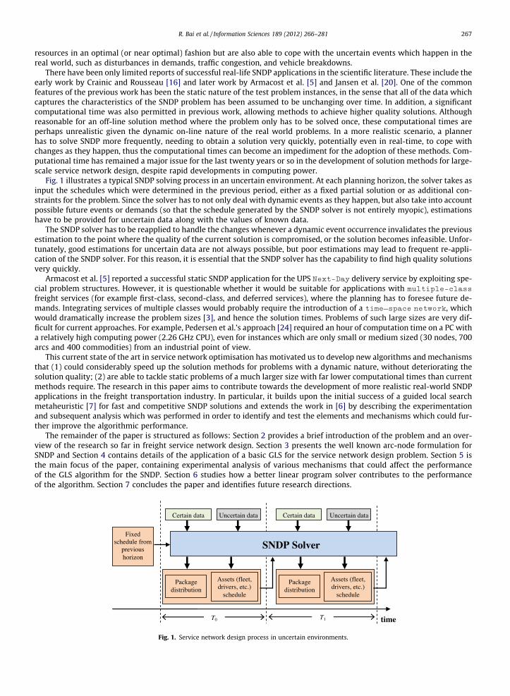
Fig. 1 illustrates a typical SNDP solving process in an uncertain environment. At each planning horizon, the solver takes asinput the schedules which were determined in the previous period, either as a fixed partial solution or as additional con-straints for the problem. Since the solver has to not only deal with dynamic events as they happen, but also take into accountpossible future events or demands (so that the schedule generated by the SNDP solver is not entirely myopic), estimationshave to be provided for uncertain data along with the values of known data.

The SNDP solver has to be reapplied to handle the changes whenever a dynamic event occurrence invalidates the previousestimation to the point where the quality of the current solution is compromised, or the solution becomes infeasible. Unfor-tunately, good estimations for uncertain data are not always possible, but poor estimations may lead to frequent re-appli-cation of the SNDP solver. For this reason, it is essential that the SNDP solver has the capability to find high quality solutionsvery quickly.

Armacost et al. [5] reported a successful static SNDP application for the UPS Next-Day delivery service by exploiting spe-cial problem structures. However, it is questionable whether it would be suitable for applications with multiple-class

freight services (for example first-class, second-class, and deferred services), where the planning has to foresee future de-mands. Integrating services of multiple classes would probably require the introduction of a time–space network, whichwould dramatically increase the problem sizes [3], and hence the solution times. Problems of such large sizes are very dif-ficult for current approaches. For example, Pedersen et al.’s approach [24] required an hour of computation time on a PC witha relatively high computing power (2.26 GHz CPU), even for instances which are only small or medium sized (30 nodes, 700arcs and 400 commodities) from an industrial point of view.

This current state of the art in service network optimisation has motivated us to develop new algorithms and mechanismsthat (1) could considerably speed up the solution methods for problems with a dynamic nature, without deteriorating thesolution quality; (2) are able to tackle static problems of a much larger size with far lower computational times than currentmethods require. The research in this paper aims to contribute towards the development of more realistic real-world SNDPapplications in the freight transportation industry. In particular, it builds upon the initial success of a guided local searchmetaheuristic [7] for fast and competitive SNDP solutions and extends the work in [6] by describing the experimentationand subsequent analysis which was performed in order to identify and test the elements and mechanisms which could fur-ther improve the algorithmic performance.

The remainder of the paper is structured as follows: Section 2 provides a brief introduction of the problem and an over-view of the research so far in freight service network design. Section 3 presents the well known arc-node formulation forSNDP and Section 4 contains details of the application of a basic GLS for the service network design problem. Section 5 isthe main focus of the paper, containing experimental analysis of various mechanisms that could affect the performanceof the GLS algorithm for the SNDP. Section 6 studies how a better linear program solver contributes to the performanceof the algorithm. Section 7 concludes the paper and identifies future research directions.

time T0 T1

Fixed schedule from

previous horizon

SNDP Solver

Certain data Uncertain data

Assets (fleet, drivers, etc.)

schedule

Package distribution

Assets (fleet, drivers, etc.)

schedule

Package distribution

Certain data Uncertain data

Fig. 1. Service network design process in uncertain environments.

268 R. Bai et al. / Information Sciences 189 (2012) 266–281

2. Problem description and literature review

The service network design problem (SNDP) is an important tactical/operational freight transportation planning problem.It is of particular interest for less-than-truckload (LTL) transportation and express delivery services, where consolidation ofdeliveries is widely adopted in order to maximise the utilisation of freight resources [12]. The problem is usually concernedwith finding a cost-minimising transportation network configuration that satisfies the delivery requirements for all of thecommodities, each of which is defined by a source node, target node, and quantity of demand. More specifically, the servicenetwork design problem involves the search for optimal decisions in terms of the service characteristics (for example, theselection of routes to utilise and the vehicle types for each route, the service frequency and the delivery timetables), the flowdistribution paths for each commodity, the consolidation policies, and the idle vehicle re-positioning, so that legal, social andtechnical requirements are met [27].

The service network design problem is similar to the capacitated multicommodity network design (CMND) problem ex-cept that the SNDP has an extra degree of complexity due to the required balance constraint for freight assets (for example,ensuring that vehicle routes are contiguous and that vehicles are in the correct positions after each planning cycle), whichdoes not apply to the standard CMND. Both the CMND and the SNDP are known to be NP-Hard problems [18]. The remainderof this section provides a brief overview of the previous research into service network design. More comprehensive reviewscan be found in [12,15,27].

Service network design is closely related to the classic network flow problems [1]. Early work in this field includes[16,25,17]. Crainic et al. [14] applied a tabu search metaheuristic to the container allocation/positioning problem and Crainicet al. [13] investigated a hybrid approach for CMND, combining a tabu search method with pivot-like neighbourhood movesand column generation. Ghamlouche et al. [18] continued the work and proposed a more efficient cycle-based neighbour-hood structure for CMND. Experimental tests, within a simple tabu search framework, demonstrated the superiority ofthe method to the earlier pivot-like neighbourhood moves in [13]. This approach was later enhanced by adopting a path-relinking mechanism [19].

Barnhart and her research team [9,21] addressed a real-life air cargo express delivery service network design problem.The problem is characterised by its large problem sizes and the addition of further complex constraints to those whichare in existence in the general SNDP model. A tree formulation was introduced and the problem was solved heuristicallyusing a method based upon column generation. Armacost et al. [4] introduced a new mathematical model based on an inno-vative concept called the composite variable, which has a better LP bound than other models. A column generation meth-od using this new model was able to solve the problem successfully within a reasonable computational time, takingadvantage of the specific problem details. However, it may be difficult to generalise the model to other freight transportationapplications, especially when there are several classes of services being planned simultaneously.

Recent work by Pederson et al. [24] studied more generic service network design models in which the asset balance con-straint was present. A multi-start metaheuristic, based on tabu search, was developed and tested on a set of benchmark in-stances. The tabu search method outperformed a commercial MIP solver when computational time was limited to one hourper instance on a test PC with a Pentium IV 2.26 GHz CPU. Andersen et al. [3] compared the node-arc based formulation, thepath-based formulation and a cycle-based formulation for SNDP problems. Computational results on a set of small randomlygenerated instances indicated that the cycle-based formulation gave significantly stronger bounds than the other two andhence may lead to much faster solution of problems. More recent work by Bai et al. [7] attempted to further reduce the com-putational time and investigated a guided local search approach. The computational study, based on a set of popular bench-mark instances, showed that the guided local search, if configured appropriately, was able to obtain solutions of a similarquality level to the tabu search but with only two thirds of the computational time, even when executed on a slightly slowermachine. Barcos et al. [8] investigated an ant colony optimization (ACO) approach to address a variant (simplified) freightservice network design problem. The algorithm was able to obtain solutions better than those adopted in the real-worldwithin a reasonable computational time. Andersen et al. [2] studied a branch and price method for the service network de-sign problem. Although the proposed algorithm was able to find solutions of higher quality than the previous methods, the10-hour computational time required by the algorithm poses a great challenge for its practical applications. Chiou [11] pro-posed a two-level mathematical programming model for the logistics network design. The upper level model is concernedwith optimising the network configuration while the lower level optimises the flow distribution with flow-dependent mar-ginal costs. However, the model does not take into account the asset balance constraints.

The research mentioned above primarily dealt with problems of a static nature. However, service network planning in-volves several uncertain aspects, such as unpredictable demands, traffic congestion, delays, and vehicle breakdowns. Opti-mal solutions for a static problem may turn out to have poor quality or even lose feasibility as a result of the unpredictabledynamic events. Liu et al. [22] proposed a two-stage approach based on stochastic programming to model the interdepen-dencies between transportation assets and potential uncertainties. Bock [10] proposed a dynamic scheduling like approachto deal with uncertainties. From an initial plan, which was generated using estimated data, the system dynamically re-solvedthe current plan in order to adapt to the evolving problem, so the SNDP had to be solved repeatedly. Due to the lack of pre-dictability for the data, we have adopted the latter type of approach, focusing upon speed of execution to allow the algorithmto be re-executed as the situation changes, however introducing some elements of stochastic programming would be aninteresting area for future research.


The goal of this paper is to develop a much more efficient algorithm which could be utilised in conjunction with existingtechnologies, such as parallel computing, to allow the solution of much larger scale SNDP instances (of the type which oftenoccur when using the time–space network formulation) or of dynamic SNDP problems where the computational time is crit-ical. This paper contributes to the literature not only a more efficient hybrid metaheuristic approach for the SNDP, but moreimportantly, an experimental evaluation of the behaviour and performance of several effective components and mechanismswithin a GLS framework. We expect that these findings will also be useful for other researchers working on similaralgorithms.

3. Freight service network design problem (SNDP) model

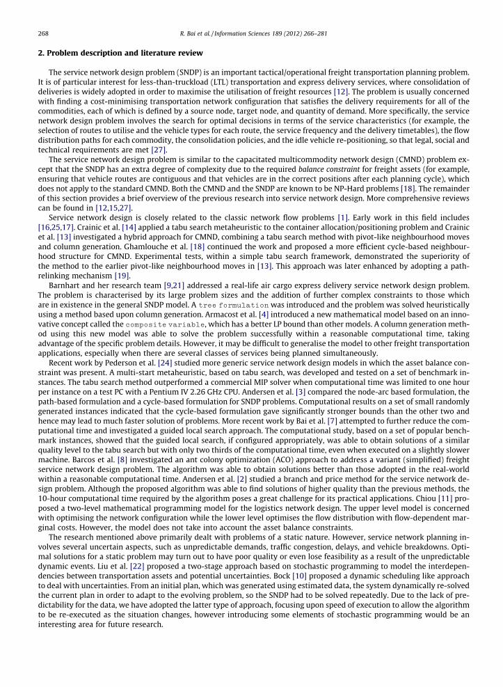
We focus on a specific, recently studied service network design formulation which was described in [24] and which wealso present here for completeness. A summary list of the notations used in the model is provided in Table 1 and the model isdiscussed below.

Let G ¼ ðN;AÞ denote a directed graph with nodes N and arcs A. Let (i, j) denote the arc from node i to node j. Let K bethe set of commodities. For each commodity k 2K, let o(k) and s(k) denote its origin and destination nodes, respectively. Letyij be boolean decision variables, where yij = 1 if arc(i, j) is used in the final design and 0 otherwise. Let xk

ij denote the flow ofcommodity k on arc(i, j). Let uij and fij be the capacity and fixed cost, respectively, for arc(i, j). Finally, let ck

ij denote the variablecost of moving one unit of commodity k along arc(i, j).

The service network design problem can then be formulated as follows:

Table 1List of n

Nota

N

A

G ¼ði; jÞuij

fij

K

o(k)s(k)dk

ckij

xkij

yij

x

yNþðN�ðbk

i

z(x,yg(s),

minimise zðx; yÞ ¼Xði;jÞ2A

fijyij þXk2K

Xði;jÞ2A

ckijx

kij ð1Þ

subject toXk2K

xkij 6 uijyij 8ði; jÞ 2A ð2Þ

Xj2NþðiÞ

xkij �

Xj2N�ðiÞ

xkji ¼ bk

i 8i 2N; 8k 2K ð3Þ

Xj2N�ðiÞ

yji �X

j2NþðiÞyij ¼ 0 8i 2N ð4Þ

where xkij P 0 and yij 2 {0,1} are the decision variables. The network capacity constraint (2) ensures that the maximum flow

along each arc(i, j) is limited by the arc capacity. The flow conservation constraint (3) ensures that the entire flow of eachcommodity is delivered to its destination, where NþðiÞ denotes the set of outward neighbours of node i and N�ðiÞ theset of inward neighbours. bk

i is the outward flow of commodity k for node i, so we set bki ¼ dk if i ¼ oðkÞ; bk

i ¼ �dk ifi = s(k), and bk

i ¼ 0 otherwise. Constraint (4) is the asset-balance constraint, which is missing from the standard CMND formu-lation, as previously discussed, and which ensures the balance of transportation assets (i.e. vehicles) at the end of each plan-ning period.

otations used in the SNDP model.

tion Meaning

The set of nodesThe set of arcs in the network

ðN;AÞ Directed graph with nodes N and arcs A

2A The arc from node i to jCapacity of arc(i, j)The fixed cost of arc(i, j)The set of commoditiesThe origin for commodity k 2K

The sink (destination) for commodity kThe flow demand of commodity kThe variable cost for shipping a unit of commodity k on the arc(i, j)

The amount of flow of commodity k on the arc (i, j) in a solution

The network design variables. yij = 1 if arc(i, j) is open in a solution and 0 otherwiseThe vector of all flow decision variables, i.e. x ¼ hx0

00 ; . . . ; xkij; . . .i

The vector of all design variables, i.e. y = hy00, . . . ,yij, . . .iiÞ The set of outward neighbouring nodes of node iiÞ The set of incoming neighbouring nodes of node i

The outward flow of commodity k:bki ¼ dk if i ¼ oðkÞ; bk

i ¼ �dk if i = s(k) and 0 otherwise) The objective of SNDP model, which represents the sum of the fixed cost and the variable cost for given solution vectors x and yg(x,y) A transformed objective function for the SNDP problem, containing a penalty term for solution infeasibility, expressed in terms of

potential solution s or the decision variable component vectors x and y of s


For a given set of design variables �y ¼ hy00; . . . ; yij; . . .i, the problem becomes one of finding the optimal flow distributionvariables. Constraint (4) is no longer relevant and the flow must be zero on all closed arcs, so only open arcs have to be con-

sidered in the model. Let A denote the set of open arcs in the design vector �y, then flow distribution variables xkij

� �for all

open arcs (ði; jÞ 2A) can be obtained by solving the following capacitated multicommodity min-cost flow problem (CMMCF),where xk

ij P 0 8ði; jÞ 2A; k:

minimise �zðxÞ ¼Xk2K

Xði;jÞ2A

ckijx

kij ð5Þ

subject toXk2K

xkij 6 uij 8ði; jÞ 2A ð6Þ

Xj2NþðiÞ

xkij �

Xj2N�ðiÞ

xkji ¼ bk

i ; 8i 2N; 8k 2K ð7Þ

It was shown in [7] that a multi-start guided local search (GLS) approach performed well on this problem, producing re-sults which were competitive with a recently proposed tabu search method [24], but in a much lower computational time.Based upon this initial success, this research aims to investigate, in detail, what contributed to this success and whetherthere are components and mechanisms that may lead to further improvement either in terms of computational time or solu-tion quality. In particular, we have investigated: (a) how effectively the current GLS explores the search space rather thangetting stuck in a set of locally optimal solutions; (b) whether more efficient mechanisms can be found and integrated withinGLS; (c) other factors which could potentially reduce the search time.

4. Guided local search for SNDP

4.1. Guided local search

Guided local search (GLS) is a metaheuristic which was designed for constraint satisfaction and combinatorial optimisa-tion problems [26]. Like tabu search, GLS makes use of information gathered during the search to guide it and enable it toescape locally optimal regions, rather than cycling between a few locally good solutions. In addition, GLS also exploits do-main knowledge by penalising ‘‘unpopular’’ features in a candidate solution. The core of the guided local search methodis the identification of a set of features and the determination of a transformed evaluation function. For a given solutions, the transformed evaluation function will have the following form:

EðsÞ ¼ gðsÞ þ GLS pen ¼ gðsÞ þ k�X

r

ðpr � IrðsÞÞ ð8Þ

where g(s) is the original objective function. The formulations g(s) and g(x,y) are used interchangeably in this paper, sincefunction g could be expressed in terms of the entire solution s or in terms of the vectors x and y of decision variables, as in Eq.(9).

The variable pr is the current penalty for the presence of a given feature r in the current solution s, and Ir(s) is an indicatorvariable such that Ir(s) = 1 if the candidate solution s contains feature r and Ir(s) = 0 otherwise. GLS_pen is, therefore, thescaled (by k) penalty summation which is applied by the GLS. k is a control parameter which is often estimated byk ¼ a� gðs�Þ

PrIrðs�Þ

�where s⁄ is the current best solution and a is a parameter that is less problem-dependent than k.

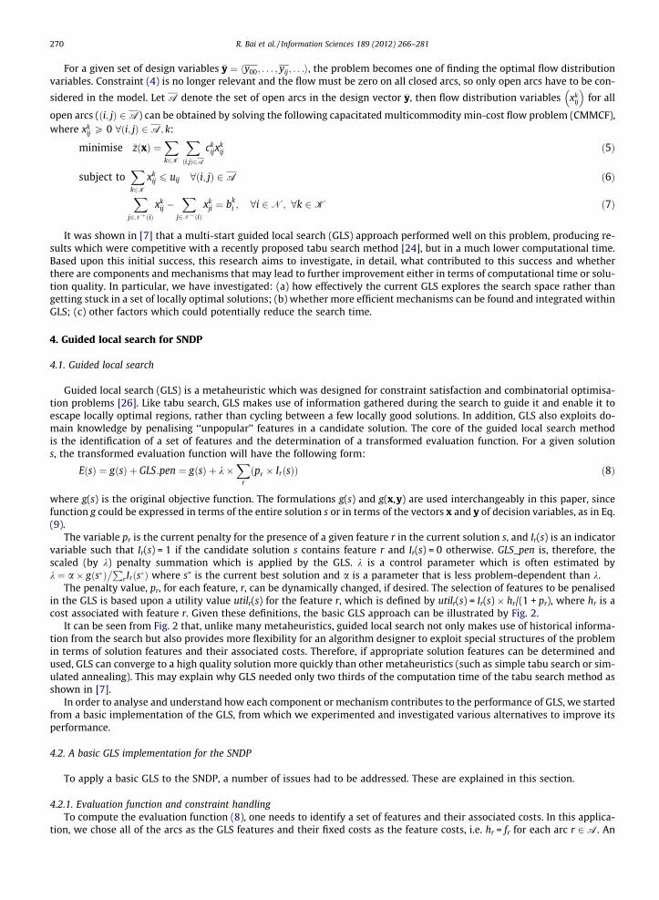
The penalty value, pr, for each feature, r, can be dynamically changed, if desired. The selection of features to be penalisedin the GLS is based upon a utility value utilr(s) for the feature r, which is defined by utilr(s) = Ir(s) � hr/(1 + pr), where hr is acost associated with feature r. Given these definitions, the basic GLS approach can be illustrated by Fig. 2.

It can be seen from Fig. 2 that, unlike many metaheuristics, guided local search not only makes use of historical informa-tion from the search but also provides more flexibility for an algorithm designer to exploit special structures of the problemin terms of solution features and their associated costs. Therefore, if appropriate solution features can be determined andused, GLS can converge to a high quality solution more quickly than other metaheuristics (such as simple tabu search or sim-ulated annealing). This may explain why GLS needed only two thirds of the computation time of the tabu search method asshown in [7].

In order to analyse and understand how each component or mechanism contributes to the performance of GLS, we startedfrom a basic implementation of the GLS, from which we experimented and investigated various alternatives to improve itsperformance.

4.2. A basic GLS implementation for the SNDP

To apply a basic GLS to the SNDP, a number of issues had to be addressed. These are explained in this section.

4.2.1. Evaluation function and constraint handlingTo compute the evaluation function (8), one needs to identify a set of features and their associated costs. In this applica-

tion, we chose all of the arcs as the GLS features and their fixed costs as the feature costs, i.e. hr = fr for each arc r 2A. An

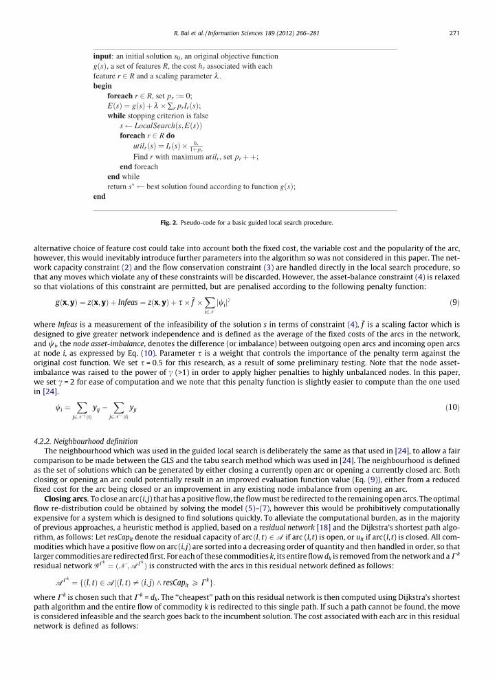
Fig. 2. Pseudo-code for a basic guided local search procedure.


alternative choice of feature cost could take into account both the fixed cost, the variable cost and the popularity of the arc,however, this would inevitably introduce further parameters into the algorithm so was not considered in this paper. The net-work capacity constraint (2) and the flow conservation constraint (3) are handled directly in the local search procedure, sothat any moves which violate any of these constraints will be discarded. However, the asset-balance constraint (4) is relaxedso that violations of this constraint are permitted, but are penalised according to the following penalty function:

gðx; yÞ ¼ zðx; yÞ þ Infeas ¼ zðx; yÞ þ s� �f �Xi2Njwij

c ð9Þ

where Infeas is a measurement of the infeasibility of the solution s in terms of constraint (4), �f is a scaling factor which isdesigned to give greater network independence and is defined as the average of the fixed costs of the arcs in the network,and wi, the node asset-imbalance, denotes the difference (or imbalance) between outgoing open arcs and incoming open arcsat node i, as expressed by Eq. (10). Parameter s is a weight that controls the importance of the penalty term against theoriginal cost function. We set s = 0.5 for this research, as a result of some preliminary testing. Note that the node asset-imbalance was raised to the power of c (>1) in order to apply higher penalties to highly unbalanced nodes. In this paper,we set c = 2 for ease of computation and we note that this penalty function is slightly easier to compute than the one usedin [24].

wi ¼X

j2NþðiÞyij �

Xj2N�ðiÞ

yji ð10Þ

4.2.2. Neighbourhood definitionThe neighbourhood which was used in the guided local search is deliberately the same as that used in [24], to allow a fair

comparison to be made between the GLS and the tabu search method which was used in [24]. The neighbourhood is definedas the set of solutions which can be generated by either closing a currently open arc or opening a currently closed arc. Bothclosing or opening an arc could potentially result in an improved evaluation function value (Eq. (9)), either from a reducedfixed cost for the arc being closed or an improvement in any existing node imbalance from opening an arc.

Closing arcs. To close an arc(i, j) that has a positive flow, the flow must be redirected to the remaining open arcs. The optimalflow re-distribution could be obtained by solving the model (5)–(7), however this would be prohibitively computationallyexpensive for a system which is designed to find solutions quickly. To alleviate the computational burden, as in the majorityof previous approaches, a heuristic method is applied, based on a residual network [18] and the Dijkstra’s shortest path algo-rithm, as follows: Let resCaplt denote the residual capacity of arcðl; tÞ 2A if arc (l, t) is open, or ult if arc(l, t) is closed. All com-modities which have a positive flow on arc(i, j) are sorted into a decreasing order of quantity and then handled in order, so thatlarger commodities are redirected first. For each of these commodities k, its entire flow dk is removed from the network and a Ck

residual network GCk ¼ ðN;ACk Þ is constructed with the arcs in this residual network defined as follows:

ACk ¼ fðl; tÞ 2Ajðl; tÞ – ði; jÞ ^ resCaplt P Ckg:

where Ck is chosen such that Ck = dk. The ‘‘cheapest’’ path on this residual network is then computed using Dijkstra’s shortestpath algorithm and the entire flow of commodity k is redirected to this single path. If such a path cannot be found, the moveis considered infeasible and the search goes back to the incumbent solution. The cost associated with each arc in this residualnetwork is defined as follows:

1 In tin the C


cClt ¼

flt þ clt � dk if ðl; tÞ 2ACkis closed;

clt � dk if ðl; tÞ 2ACkis open:

(ð11Þ

The above flow redistribution is performed in turn for each commodity that has a positive flow on arc(i, j). If the proce-dure fails to redistribute the flow for any of them then the arc closing procedure is terminated and the move is consideredinfeasible.

Opening arcs. Although opening an arc will increase the objective value due to the addition of the fixed cost for the addedarc, it could potentially reduce the node imbalance penalty and hence lead to more feasible solutions. The optimal flow dis-tribution probably changes when a closed arc is opened. However, re-solving the CMMCF model in order to determine theoptimal flow distribution would be computationally prohibitive. Therefore, in this research the flow distribution is main-tained when an arc is opened, with the only change being the addition of the incurred fixed cost of this arc and the potentialfor increased feasibility.

4.2.3. Algorithm overviewStarting from the current incumbent solution, the algorithm considers every neighbouring solution which can be gener-

ated using the opening and closing arc moves. The best solution in terms of GLS evaluation function (8) from this neighbour-hood is then adopted as the new current solution, even if it is worse than the current incumbent solution. One of theproblems which has to be faced by this kind of algorithm is that it is possible to cycle within a limited number of solutionswithin the search space, for instance a sequence of solutions such that each solution in the sequence is the best solution inthe neighbourhood of the previous solution and the first and last solutions are identical. In particular, it is important to avoidtwo-solution cycles where each is the best solution in the neighbourhood of the other.

Since opening or closing a path involves opening or closing several arcs and in each case the flow is heuristically re-allo-cated (as in [24], which this work extends), the resulting solutions provide only approximations (although they are upperbounds) for the optimal cost for that network configuration. Before proceeding with the next iteration, the CMMCF modelis solved.1 for the adopted solution, in order to find the optimal flows. The ways in which this algorithm has been adaptedand extended will be seen in more detail later.

5. Analysis of the GLS extensions

In this section, we analyse and investigate various mechanisms for extending and improving the basic GLS algorithms, inisolation, in order to understand which of these elements contributes to the superior performance of the GLS against themulti-start tabu search method utilised in [24]. The mechanisms that we consider here are the aspiration criterion, memorylength and tabu list for cycling prevention. We describe them one by one in the following subsections.

To be clear, the feasibility repair procedure, which is described later in this paper, is not applied at this stage, since thepurpose of this section is primarily to study the behaviour of each mechanism. Since there is no random element to any ofthese GLS extensions, each instance only had to be executed once.

5.1. Aspiration criteria in GLS

One of the strengths of the guided local search is its ability to use a penalty function to take advantage of domain specificinformation as well as information gathered during the search. The penalty function punishes ‘‘unpopular’’ features presentin a candidate solution. The popularity of a feature is determined by a combination of the pre-determined associated cost(utilising domain specific information) and the accumulated penalty values during the search, as explained in Section 4.2.1.

Although this penalty function is, in general, effective in guiding the search to escape from locally optimal regions, con-flicts between the objective function and the penalty function mean that it could miss some high quality solutions, since agood solution with respect to the original objective (1) is not necessarily so with respect to the evaluation function (8). Wetherefore incorporated an aspiration criterion into the basic GLS method so that the search will adopt a candidate solution ifit improves the current best solution in terms of the evaluation function g(x,y), even if its augmented objective (i.e. E(s)) isworse than that of other neighbouring solutions. Fig. 3 plots the values of the solutions which were adopted at each iterationfor the test instance C50 for both the basic GLS and the GLS with the aspiration criterion. It appears that, when given a longerexecution time, the GLS with the aspiration criterion was able to perform better than the basic GLS on average at the middleand later stages of the search, while the GLS without aspiration criteria was able to find a better overall-best-solution. How-ever, both versions of GLS found a best solution at an early stage in the search and failed to improve upon it later. This sug-gests that the penalty assignments used in the guided local search become ineffective after a certain number of iterations.

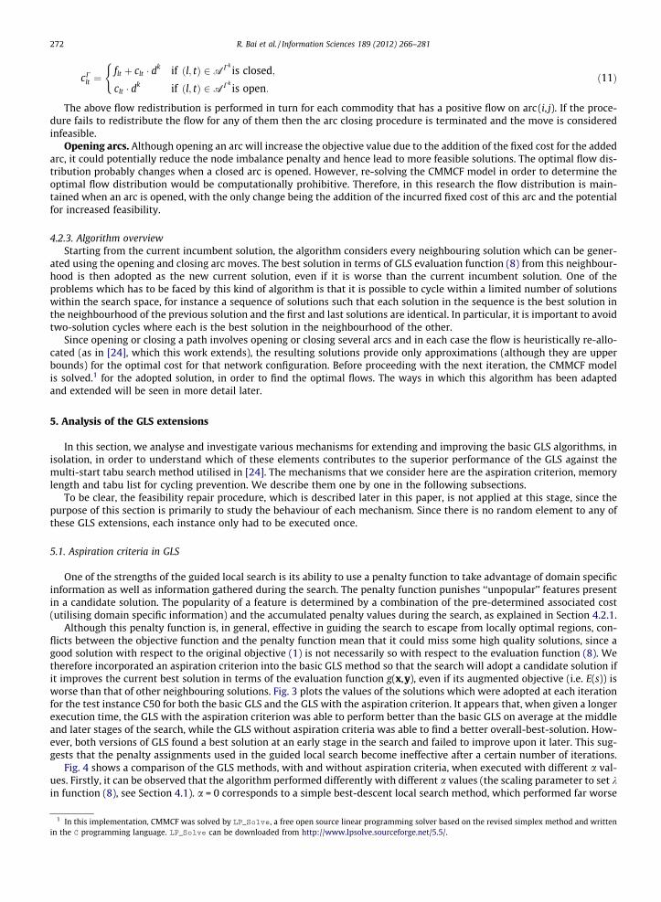
Fig. 4 shows a comparison of the GLS methods, with and without aspiration criteria, when executed with different a val-ues. Firstly, it can be observed that the algorithm performed differently with different a values (the scaling parameter to set kin function (8), see Section 4.1). a = 0 corresponds to a simple best-descent local search method, which performed far worse

his implementation, CMMCF was solved by LP_Solve, a free open source linear programming solver based on the revised simplex method and writtenprogramming language. LP_Solve can be downloaded from http://www.lpsolve.sourceforge.net/5.5/.

http://www.lpsolve.sourceforge.net/5.5/

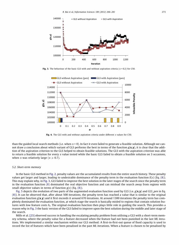
Fig. 3. The behaviour of the basic GLS with and without aspiration criteria (a = 0.2) for C50.

Fig. 4. The GLS with and without aspiration criteria under different a values for C50.


than the guided local search methods (i.e. when a > 0). In fact it even failed to generate a feasible solution. Although we can-not draw a conclusion about which variant of GLS performs the best in terms of the function g(x,y), it is clear that the addi-tion of the aspiration criterion to the GLS helped to obtain feasible solutions. The GLS with the aspiration criterion was ableto return a feasible solution for every a value tested while the basic GLS failed to obtain a feasible solution on 3 occasions,when a was relatively large (a P 0.7).

5.2. Short-term memory

In the basic GLS method in Fig. 2, penalty values are the accumulated results from the entire search history. These penaltyvalues get larger and larger, leading to undesirable dominance of the penalty term in the evaluation function E(s) (Eq. (8)).This may explain why, in Fig. 3, GLS failed to improve the best solution in the later stages of the search since the penalty termin the evaluation function (8) dominated the real objective function and can mislead the search away from regions withsmall objective values in terms of function g(s) (Eq. (8)).

Fig. 5 depicts the evolution of two parts of the augmented evaluation function used by GLS (i.e. g(x,y) and GLS_pen in Eq.(8)). It can be observed that, after about 500 iterations, the penalty term has reached a value that is similar to the originalevaluation function g(x,y) and it first exceeds it around 670 iterations. At around 1300 iterations the penalty term has com-pletely dominated the evaluation function, at which stage the search is basically misled to regions that contain solution fea-tures with low feature costs hr. The original evaluation function then plays little role in guiding the search. This provides areason why in Fig. 3 the basic version of the GLS failed to improve upon the best solution during the middle and later stage ofthe search.

Mills et al. [23] observed success in handling the escalating penalty problem from utilising a GLS with a short-term mem-ory schema, where the penalty value for a feature decreased when the feature had not been punished in the last ML itera-tions. We implemented a similar mechanism within our GLS method: A first-in-first-out queue of fixed capacity is used torecord the list of features which have been penalised in the past ML iterations. When a feature is chosen to be penalised by

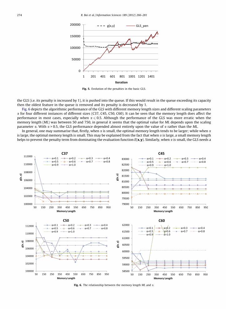
Fig. 5. Evolution of the penalties in the basic GLS.


the GLS (i.e. its penalty is increased by 1), it is pushed into the queue. If this would result in the queue exceeding its capacitythen the oldest feature in the queue is removed and its penalty is decreased by 1.

Fig. 6 depicts the algorithmic performance of the GLS with different memory length sizes and different scaling parametersa for four different instances of different sizes (C37, C45, C50, C60). It can be seen that the memory length does affect theperformance in most cases, especially when a 6 0.5. Although the performance of the GLS was more erratic when thememory length (ML) was between 50 and 750, in general it seems that the optimal value for ML depends upon the scalingparameter a. With a > 0.5, the GLS performance depended almost entirely upon the value of a rather than the ML.

In general, one may summarise that, firstly, when a is small, the optimal memory length tends to be larger; while when ais large, the optimal memory length is small. This may be explained from the fact that when a is large, a small memory lengthhelps to prevent the penalty term from dominating the evaluation function E(x,y). Similarly, when a is small, the GLS needs a

Fig. 6. The relationship between the memory length ML and a.

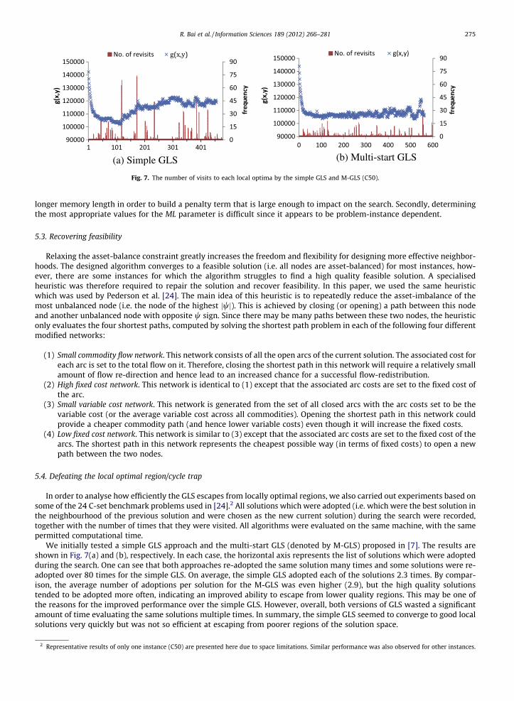
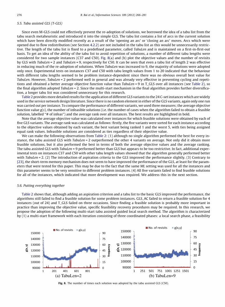
Fig. 7. The number of visits to each local optima by the simple GLS and M-GLS (C50).


longer memory length in order to build a penalty term that is large enough to impact on the search. Secondly, determiningthe most appropriate values for the ML parameter is difficult since it appears to be problem-instance dependent.

5.3. Recovering feasibility

Relaxing the asset-balance constraint greatly increases the freedom and flexibility for designing more effective neighbor-hoods. The designed algorithm converges to a feasible solution (i.e. all nodes are asset-balanced) for most instances, how-ever, there are some instances for which the algorithm struggles to find a high quality feasible solution. A specialisedheuristic was therefore required to repair the solution and recover feasibility. In this paper, we used the same heuristicwhich was used by Pederson et al. [24]. The main idea of this heuristic is to repeatedly reduce the asset-imbalance of themost unbalanced node (i.e. the node of the highest jwj). This is achieved by closing (or opening) a path between this nodeand another unbalanced node with opposite w sign. Since there may be many paths between these two nodes, the heuristiconly evaluates the four shortest paths, computed by solving the shortest path problem in each of the following four differentmodified networks:

(1) Small commodity flow network. This network consists of all the open arcs of the current solution. The associated cost foreach arc is set to the total flow on it. Therefore, closing the shortest path in this network will require a relatively smallamount of flow re-direction and hence lead to an increased chance for a successful flow-redistribution.

(2) High fixed cost network. This network is identical to (1) except that the associated arc costs are set to the fixed cost ofthe arc.

(3) Small variable cost network. This network is generated from the set of all closed arcs with the arc costs set to be thevariable cost (or the average variable cost across all commodities). Opening the shortest path in this network couldprovide a cheaper commodity path (and hence lower variable costs) even though it will increase the fixed costs.

(4) Low fixed cost network. This network is similar to (3) except that the associated arc costs are set to the fixed cost of thearcs. The shortest path in this network represents the cheapest possible way (in terms of fixed costs) to open a newpath between the two nodes.

5.4. Defeating the local optimal region/cycle trap

In order to analyse how efficiently the GLS escapes from locally optimal regions, we also carried out experiments based onsome of the 24 C-set benchmark problems used in [24].2 All solutions which were adopted (i.e. which were the best solution inthe neighbourhood of the previous solution and were chosen as the new current solution) during the search were recorded,together with the number of times that they were visited. All algorithms were evaluated on the same machine, with the samepermitted computational time.

We initially tested a simple GLS approach and the multi-start GLS (denoted by M-GLS) proposed in [7]. The results areshown in Fig. 7(a) and (b), respectively. In each case, the horizontal axis represents the list of solutions which were adoptedduring the search. One can see that both approaches re-adopted the same solution many times and some solutions were re-adopted over 80 times for the simple GLS. On average, the simple GLS adopted each of the solutions 2.3 times. By compar-ison, the average number of adoptions per solution for the M-GLS was even higher (2.9), but the high quality solutionstended to be adopted more often, indicating an improved ability to escape from lower quality regions. This may be one ofthe reasons for the improved performance over the simple GLS. However, overall, both versions of GLS wasted a significantamount of time evaluating the same solutions multiple times. In summary, the simple GLS seemed to converge to good localsolutions very quickly but was not so efficient at escaping from poorer regions of the solution space.

2 Representative results of only one instance (C50) are presented here due to space limitations. Similar performance was also observed for other instances.


5.5. Tabu assisted GLS (T-GLS)

Since even M-GLS could not effectively prevent the re-adoption of solutions, we borrowed the idea of a tabu list from thetabu search metaheuristic and introduced it into the simple GLS. The tabu list contains a list of arcs in the current solutionwhich have been directly modified recently as a result of the ‘opening an arc’ or ‘closing an arc’ moves. Arcs which wereopened due to flow redistribution (see Section 4.2.2) are not included in the tabu list as this would be unnecessarily restric-tive. The length of the tabu list is fixed to a predefined parameter, called TabuLen and is maintained on a first-in-first-outbasis. To get an idea of the ability of the tabu list to avoid repetition of solutions, a number of different tabu lengths wereconsidered for two sample instances (C37 and C50). Fig. 8(a) and (b) plot the objective values and the number of revisitsby GLS with TabuLen = 2 and TabuLen = 9, respectively for C50. It can be seen that even a tabu list of length 2 was effectivein reducing much of the re-adoption of solutions. When TabuLen was increased to 9, the majority of solutions were adoptedonly once. Experimental tests on instances C37 and C50 with tabu length values from 1 to 20 indicated that the behaviourwith different tabu lengths seemed to be problem instance-dependent since there was no obvious overall best value forTabuLen. However, TabuLen = 2 performed well in general and was already very effective in preventing cycling and repeti-tions and obtained a better average objective function value than TabuLen = 9 in T_GLS over all instances (see Table 2), sothe final algorithm adopted TabuLen = 2. Since the multi-start mechanism in the final algorithm provides further diversifica-tion, a longer tabu list was considered unnecessary for this research.

Table 2 provides more detailed results for the application of different GLS variants to the 24 C-set instances which are widelyused in the service network design literature. Since there is no random element in either of the GLS variants, again only one runwas carried out per instance. To compare the performance of different variants, we used three measures; the average objectivefunction value g(s), the number of infeasible solutions (i.e. the number of cases when the algorithm failed to obtain a feasiblesolution, labelled ‘‘# of infeas’’) and the average rank over all instances. The best results are highlighted in bold.

Note that the average objective value was calculated over instances for which feasible solutions were obtained by each offive GLS variants. The average rank was calculated as follows: firstly, the five variants were sorted for each instance accordingto the objective values obtained by each variant, the best variant being ranked 1 and the worst 5, with ties being assignedequal rank values. Infeasible solutions are considered as ties regardless of their objective value.

We can make the following observations from Table 2: (1) although no single algorithm performed the best for every in-stance, the tabu assisted GLS with TabuLen = 2 outperformed the other 4 variants on average. Not only did it obtain morefeasible solutions, but it also performed the best in terms of both the average objective values and the average ranking.The tabu assisted GLS with TabuLen = 9 performed better than GLS but appears to be too restrictive. In fact, additional exper-imental tests on instances C37 and C50 with other tabu length values showed that the algorithm generally performed betterwith TabuLen = 2. (2) The introduction of aspiration criteria to the GLS improved the performance slightly. (3) Contrary to[23], the short-term memory mechanism does not seem to have improved the performance of the GLS, at least for the param-eters that were tested for this paper. This may be due to the fact that the same ML setting was used for all the instances andthis parameter seems to be very sensitive to different problem instances. (4) All five variants failed to find feasible solutionsfor all of the instances, which indicated that more development was required. We address this in the next section.

5.6. Putting everything together

Table 2 shows that, although adding an aspiration criterion and a tabu list to the basic GLS improved the performance, thealgorithms still failed to find a feasible solution for some problem instances. GLS_AC failed to return a feasible solution for 4instances (out of 24) and T_GLS failed on three occasions. Since finding a feasible solution is probably more important inpractice than improving the objective value, specific feasibility recovery procedures may be required. In this research, wepropose the adoption of the following multi-start tabu assisted guided local search method. The algorithm is characterizedby (1) a multi-start framework with each iteration consisting of three coordinated phases: a local search phase, a feasibility

Fig. 8. The number of times each solution was adopted by the tabu assisted GLS (C50).

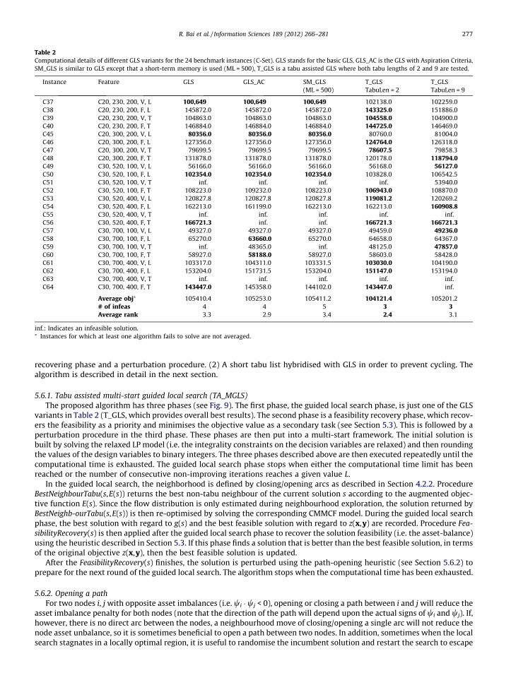
Table 2Computational details of different GLS variants for the 24 benchmark instances (C-Set). GLS stands for the basic GLS, GLS_AC is the GLS with Aspiration Criteria,SM_GLS is similar to GLS except that a short-term memory is used (ML = 500), T_GLS is a tabu assisted GLS where both tabu lengths of 2 and 9 are tested.

Instance Feature GLS GLS_AC SM_GLS T_GLS T_GLS(ML = 500) TabuLen = 2 TabuLen = 9

C37 C20, 230, 200, V, L 100,649 100,649 100,649 102138.0 102259.0C38 C20, 230, 200, F, L 145872.0 145872.0 145872.0 143325.0 151886.0C39 C20, 230, 200, V, T 104863.0 104863.0 104863.0 104558.0 104900.0C40 C20, 230, 200, F, T 146884.0 146884.0 146884.0 144725.0 146469.0C45 C20, 300, 200, V, L 80356.0 80356.0 80356.0 80760.0 81004.0C46 C20, 300, 200, F, L 127356.0 127356.0 127356.0 124764.0 126318.0C47 C20, 300, 200, V, T 79699.5 79699.5 79699.5 78607.5 79858.3C48 C20, 300, 200, F, T 131878.0 131878.0 131878.0 120178.0 118794.0C49 C30, 520, 100, V, L 56166.0 56166.0 56166.0 56168.0 56127.0C50 C30, 520, 100, F, L 102354.0 102354.0 102354.0 103828.0 106542.5C51 C30, 520, 100, V, T inf. inf. inf. inf. 53940.0C52 C30, 520, 100, F, T 108223.0 109232.0 108223.0 106943.0 108870.0C53 C30, 520, 400, V, L 120827.8 120827.8 120827.8 119081.2 120269.2C54 C30, 520, 400, F, L 162213.0 161199.0 162213.0 162213.0 160908.8C55 C30, 520, 400, V, T inf. inf. inf. inf. inf.C56 C30, 520, 400, F, T 166721.3 inf. inf. 166721.3 166721.3C57 C30, 700, 100, V, L 49327.0 49327.0 49327.0 49459.0 49236.0C58 C30, 700, 100, F, L 65270.0 63660.0 65270.0 64658.0 64367.0C59 C30, 700, 100, V, T inf. 48365.0 inf. 48125.0 47857.0C60 C30, 700, 100, F, T 58927.0 58188.0 58927.0 58603.0 58428.0C61 C30, 700, 400, V, L 103317.0 104311.0 103331.5 103030.0 104190.0C62 C30, 700, 400, F, L 153204.0 151731.5 153204.0 151147.0 153194.0C63 C30, 700, 400, V, T inf. inf. inf. inf. inf.C64 C30, 700, 400, F, T 143447.0 145358.0 144102.0 143447.0 inf.

Average obj⁄ 105410.4 105253.0 105411.2 104121.4 105201.2# of infeas 4 4 5 3 3Average rank 3.3 2.9 3.4 2.4 3.1

inf.: Indicates an infeasible solution.⁄ Instances for which at least one algorithm fails to solve are not averaged.


recovering phase and a perturbation procedure. (2) A short tabu list hybridised with GLS in order to prevent cycling. Thealgorithm is described in detail in the next section.

5.6.1. Tabu assisted multi-start guided local search (TA_MGLS)The proposed algorithm has three phases (see Fig. 9). The first phase, the guided local search phase, is just one of the GLS

variants in Table 2 (T_GLS, which provides overall best results). The second phase is a feasibility recovery phase, which recov-ers the feasibility as a priority and minimises the objective value as a secondary task (see Section 5.3). This is followed by aperturbation procedure in the third phase. These phases are then put into a multi-start framework. The initial solution isbuilt by solving the relaxed LP model (i.e. the integrality constraints on the decision variables are relaxed) and then roundingthe values of the design variables to binary integers. The three phases described above are then executed repeatedly until thecomputational time is exhausted. The guided local search phase stops when either the computational time limit has beenreached or the number of consecutive non-improving iterations reaches a given value L.

In the guided local search, the neighborhood is defined by closing/opening arcs as described in Section 4.2.2. ProcedureBestNeighbourTabu(s,E(s)) returns the best non-tabu neighbour of the current solution s according to the augmented objec-tive function E(s). Since the flow distribution is only estimated during neighbourhood exploration, the solution returned byBestNeighb-ourTabu(s,E(s)) is then re-optimised by solving the corresponding CMMCF model. During the guided local searchphase, the best solution with regard to g(s) and the best feasible solution with regard to z(x,y) are recorded. Procedure Fea-sibilityRecovery(s) is then applied after the guided local search phase to recover the solution feasibility (i.e. the asset-balance)using the heuristic described in Section 5.3. If this phase finds a solution that is better than the best feasible solution, in termsof the original objective z(x,y), then the best feasible solution is updated.

After the FeasibilityRecovery(s) finishes, the solution is perturbed using the path-opening heuristic (see Section 5.6.2) toprepare for the next round of the guided local search. The algorithm stops when the computational time has been exhausted.

5.6.2. Opening a pathFor two nodes i, j with opposite asset imbalances (i.e. wi � wj < 0), opening or closing a path between i and j will reduce the

asset imbalance penalty for both nodes (note that the direction of the path will depend upon the actual signs of wi and wj). If,however, there is no direct arc between the nodes, a neighbourhood move of closing/opening a single arc will not reduce thenode asset unbalance, so it is sometimes beneficial to open a path between two nodes. In addition, sometimes when the localsearch stagnates in a locally optimal region, it is useful to randomise the incumbent solution and restart the search to escape

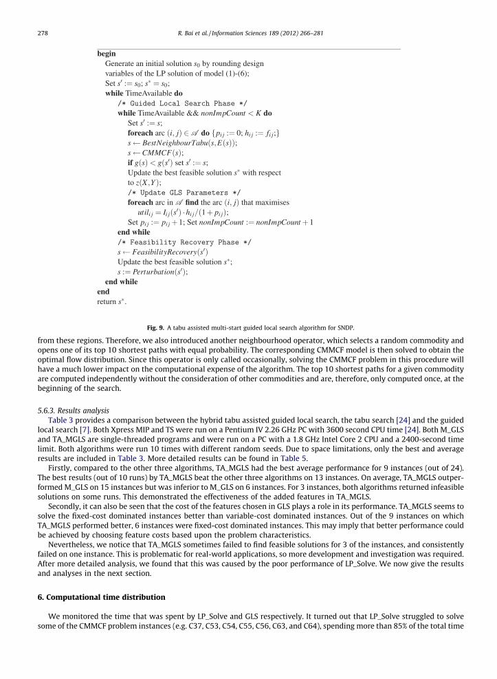
Fig. 9. A tabu assisted multi-start guided local search algorithm for SNDP.


from these regions. Therefore, we also introduced another neighbourhood operator, which selects a random commodity andopens one of its top 10 shortest paths with equal probability. The corresponding CMMCF model is then solved to obtain theoptimal flow distribution. Since this operator is only called occasionally, solving the CMMCF problem in this procedure willhave a much lower impact on the computational expense of the algorithm. The top 10 shortest paths for a given commodityare computed independently without the consideration of other commodities and are, therefore, only computed once, at thebeginning of the search.

5.6.3. Results analysisTable 3 provides a comparison between the hybrid tabu assisted guided local search, the tabu search [24] and the guided

local search [7]. Both Xpress MIP and TS were run on a Pentium IV 2.26 GHz PC with 3600 second CPU time [24]. Both M_GLSand TA_MGLS are single-threaded programs and were run on a PC with a 1.8 GHz Intel Core 2 CPU and a 2400-second timelimit. Both algorithms were run 10 times with different random seeds. Due to space limitations, only the best and averageresults are included in Table 3. More detailed results can be found in Table 5.

Firstly, compared to the other three algorithms, TA_MGLS had the best average performance for 9 instances (out of 24).The best results (out of 10 runs) by TA_MGLS beat the other three algorithms on 13 instances. On average, TA_MGLS outper-formed M_GLS on 15 instances but was inferior to M_GLS on 6 instances. For 3 instances, both algorithms returned infeasiblesolutions on some runs. This demonstrated the effectiveness of the added features in TA_MGLS.

Secondly, it can also be seen that the cost of the features chosen in GLS plays a role in its performance. TA_MGLS seems tosolve the fixed-cost dominated instances better than variable-cost dominated instances. Out of the 9 instances on whichTA_MGLS performed better, 6 instances were fixed-cost dominated instances. This may imply that better performance couldbe achieved by choosing feature costs based upon the problem characteristics.

Nevertheless, we notice that TA_MGLS sometimes failed to find feasible solutions for 3 of the instances, and consistentlyfailed on one instance. This is problematic for real-world applications, so more development and investigation was required.After more detailed analysis, we found that this was caused by the poor performance of LP_Solve. We now give the resultsand analyses in the next section.

6. Computational time distribution

We monitored the time that was spent by LP_Solve and GLS respectively. It turned out that LP_Solve struggled to solvesome of the CMMCF problem instances (e.g. C37, C53, C54, C55, C56, C63, and C64), spending more than 85% of the total time

Table 3A comparison of TA_MGLS against Xpress MIP solver, Tabu Search (TS) and Multi-start GLS (M_GLS). Results by Xpress MIP and Tabu Search were drawn from[24]. Results by M_GLS were drawn from [7]. The best results are in bold.

Inst. Feature Xpress MIP TS (1 run) M_GLS (10 runs) TA_MGLS (10 runs)

Best Average Best Average

C37 C20, 230, 200, V, L 101,112 102,919 100,771 102,311 98,798 100,774C38 C20, 230, 200, F, L 153,534 150,764 143,017 145,763 142,216 144,699C39 C20, 230, 200, V, T 105,840 103,371 103,428 104,030 103,063 104,198C40 C20, 230, 200, F, T 154,026 149,942 143,446 145,401 141,853 143,690C45 C20, 300, 200, V, L 81,184 82,533 79,020 80,764 78,787 79,692C46 C20, 300, 200, F, L 131,876 128,757 125,290 127,791 124,580 125,362C47 C20, 300, 200, V, T 78,675 78,571 77,839 78,906 77,209 78,837C48 C20, 300, 200, F, T 127,412 116,338 116,712 119,092 114,601 117,156C49 C30, 520, 100, V, L 55,138 55,981 55,437 55,806 55,422 55,869C50 C30, 520, 100, F, L n/a 104,533 99,821 102,732 100,342 102,497C51 C30, 520, 100, V, T 53,125 54,493 53,644 54,073 53,744 54,027C52 C30, 520, 100, F, T 106,761 105,167 104,753 105,924 103,996 105,451C53 C30, 520, 400, V, L n/a 119,735 119,344 121,214 117,562 118,551C54 C30, 520, 400, F, L n/a 162,360 161,731 162,373 160,339 162,480C55 C30, 520, 400, V, T n/a 120,421 122,877 593,677⁄ 4,366,710⁄ 814,149⁄

C56 C30, 520, 400, F, T n/a 161,978 165,894 552,913⁄ 165,757 1,002,886⁄

C57 C30, 700, 100, V, L 48,849 49,429 49,451 49,575 49,221 49,269C58 C30, 700, 100, F, L 65,516 63,889 63,516 64,102 62,205 63,143C59 C30, 700, 100, V, T 47,052 48,202 47,518 47,833 47,518 47,859C60 C30, 700, 100, F, T 57,447 58,204 58,017 58,563 57,673 57,938C61 C30, 700, 400, V, L n/a 103,932 103,136 103,577 103,352 103,621C62 C30, 700, 400, F, L n/a 157,043 150,449 596,588⁄ 148,809 150,867C63 C30, 700, 400, V, T n/a 103,085 103,581 537,477⁄ 103,323 784,872⁄

C64 C30, 700, 400, F, T n/a 141,917 142,575 144,135 143,717 144,368

⁄ Indicates an infeasible solution.


allowed, leaving very little time for the GLS and the feasibility recovery heuristic to search for high quality feasible solutions.To further confirm the conjecture that this was the problem, we replaced LP_Solve with CPLEX12 as the CMMCF solver andkept the remaining configuration the same. To ensure a fair comparison, the CPLEX thread count was set to 1 to prevent itusing more than one CPU core. Table 4 shows a comparison of the two variants for the benchmark instance set. It can be seenthat not only was the proposed algorithm able to find a feasible solution for every instance in every run, but in addition, boththe average and best results were considerably improved.

Table 4A comparison of LP_Solve and CPLEX as LP solvers. The best results are in bold.

Inst. TS (1 run) TA_MGLS with LP_Solve TA_MGLS with CPLEX

Best Average Lptime (%) Best Average LPtime (%)

C37 102,919 98797.8 100,774 85 98760.0 99622.2 31C38 150,764 142,216 144,699 81 142113.0 143867.0 30C39 103,371 103,063 104,198 86 102137.3 102833.1 31C40 149,942 141,853 143,690 87 141802.0 143839.5 37C45 82,533 78,787 79,692 86 79029.5 79895.4 34C46 128,757 124,580 125,362 84 121773.0 124454.3 34C47 78,571 77209.3 78,837 85 77066.0 78302.5 30C48 116,338 114,601 117,156 86 114465.0 115836.2 31C49 55,981 55,422 55,869 48 55732.0 55985.6 9C50 104,533 100,342 102,497 58 100290.0 102016.9 12C51 54,493 53,744 54027.2 58 54372.0 54707.7 11C52 105,167 103,996 105,451 61 104574.0 105422.8 11C53 119,735 117561.71 118,551 87 116196.0 116915.4 47C54 162,360 160,339 162,480 83 154941.0 156008.5 37C55 120,421 436679.8⁄ 814149.1⁄ 86 118335.7 118894.1 42C56 161,978 165757.3 1002886.0⁄ 80 157939.6 159426.5 47C57 49,429 49,221 49,269 33 49385.0 49456.9 6C58 63,889 62,205 63,143 37 62055.0 62773.6 7C59 48,202 47,518 47,859 49 47519.0 47727.8 7C60 58,204 57,673 57938.0 46 57571.0 58046.0 7C61 103,932 103352.2 103,621 75 101609.5 102215.9 21C62 157,043 148809.3 150,867 78 142563.2 144754.7 36C63 103,085 103,323 784871.7⁄ 90 98656.8 99726.1 28C64 141,917 143,717 144,368 78 135777.5 136727.1 29

⁄ Indicates an infeasible solution being returned by the algorithm.

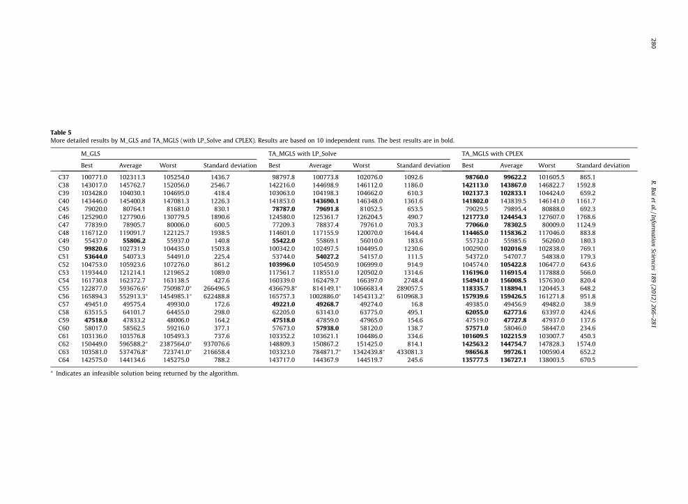
Table 5More detailed results by M_GLS and TA_MGLS (with LP_Solve and CPLEX). Results are based on 10 independent runs. The best results are in bold.

M_GLS TA_MGLS with LP_Solve TA_MGLS with CPLEX

Best Average Worst Standard deviation Best Average Worst Standard deviation Best Average Worst Standard deviation

C37 100771.0 102311.3 105254.0 1436.7 98797.8 100773.8 102076.0 1092.6 98760.0 99622.2 101605.5 865.1C38 143017.0 145762.7 152056.0 2546.7 142216.0 144698.9 146112.0 1186.0 142113.0 143867.0 146822.7 1592.8C39 103428.0 104030.1 104695.0 418.4 103063.0 104198.3 104662.0 610.3 102137.3 102833.1 104424.0 659.2C40 143446.0 145400.8 147081.3 1226.3 141853.0 143690.1 146348.0 1361.6 141802.0 143839.5 146141.0 1161.7C45 79020.0 80764.1 81681.0 830.1 78787.0 79691.8 81052.5 653.5 79029.5 79895.4 80888.0 692.3C46 125290.0 127790.6 130779.5 1890.6 124580.0 125361.7 126204.5 490.7 121773.0 124454.3 127607.0 1768.6C47 77839.0 78905.7 80006.0 600.5 77209.3 78837.4 79761.0 703.3 77066.0 78302.5 80009.0 1124.9C48 116712.0 119091.7 122125.7 1938.5 114601.0 117155.9 120070.0 1644.4 114465.0 115836.2 117046.0 883.8C49 55437.0 55806.2 55937.0 140.8 55422.0 55869.1 56010.0 183.6 55732.0 55985.6 56260.0 180.3C50 99820.6 102731.9 104435.0 1503.8 100342.0 102497.5 104495.0 1230.6 100290.0 102016.9 102838.0 769.1C51 53644.0 54073.3 54491.0 225.4 53744.0 54027.2 54157.0 111.5 54372.0 54707.7 54838.0 179.3C52 104753.0 105923.6 107276.0 861.2 103996.0 105450.9 106999.0 914.9 104574.0 105422.8 106477.0 643.6C53 119344.0 121214.1 121965.2 1089.0 117561.7 118551.0 120502.0 1314.6 116196.0 116915.4 117888.0 566.0C54 161730.8 162372.7 163138.5 427.6 160339.0 162479.7 166397.0 2748.4 154941.0 156008.5 157630.0 820.4C55 122877.0 593676.6⁄ 750987.0⁄ 266496.5 436679.8⁄ 814149.1⁄ 1066683.4 289057.5 118335.7 118894.1 120445.3 648.2C56 165894.3 552913.3⁄ 1454985.1⁄ 622488.8 165757.3 1002886.0⁄ 1454313.2⁄ 610968.3 157939.6 159426.5 161271.8 951.8C57 49451.0 49575.4 49930.0 172.6 49221.0 49268.7 49274.0 16.8 49385.0 49456.9 49482.0 38.9C58 63515.5 64101.7 64455.0 298.0 62205.0 63143.0 63775.0 495.1 62055.0 62773.6 63397.0 424.6C59 47518.0 47833.2 48006.0 164.2 47518.0 47859.0 47965.0 154.6 47519.0 47727.8 47937.0 137.6C60 58017.0 58562.5 59216.0 377.1 57673.0 57938.0 58120.0 138.7 57571.0 58046.0 58447.0 234.6C61 103136.0 103576.8 105493.3 737.6 103352.2 103621.1 104486.0 334.6 101609.5 102215.9 103007.7 450.3C62 150449.0 596588.2⁄ 2387564.0⁄ 937076.6 148809.3 150867.2 151425.0 814.1 142563.2 144754.7 147828.3 1574.0C63 103581.0 537476.8⁄ 723741.0⁄ 216658.4 103323.0 784871.7⁄ 1342439.8⁄ 433081.3 98656.8 99726.1 100590.4 652.2C64 142575.0 144134.6 145275.0 788.2 143717.0 144367.9 144519.7 245.6 135777.5 136727.1 138003.5 670.5

⁄ Indicates an infeasible solution being returned by the algorithm.

280R

.Baiet

al./Information

Sciences189

(2012)266–

281


7. Discussion and future work

In this research, we carried out experiments to look at several components and aspects that could potentially speedup theGLS approach for service network design problems. These include a tabu list, short-term memory and aspiration criteria. Inparticular, we found that in both the simple GLS and its multi-start version, time was wasted due to the repeated re-adoptionof the same solutions. We proposed a tabu assisted GLS schema within a multi-start framework to prevent this problem.Results have demonstrated the superiority of the method.

In addition, our observations showed that LP_Solve struggled on some problem instances, for which the majority ofcomputational time (more than 85%) was used when solving CMMCF problems. Our tests with CPLEX12 showed that a fasterLP solver was able to further improve the performance of our proposed method.

In future, we will investigate more neighbourhood structures in the GLS approach. In particular, we will consider multipleways for flow redirection on opening/closing an arc. In addition, if certain criteria are met, more accurate neighbourhoodevaluations may be used by applying CPLEX to solve the CMMCF problem. Another potential research direction is adoptingstochastic programming to address some of uncertainties in SNDP.

Acknowledgement

This research is supported by the National Natural Science Foundation of China (NSFC 71001055) and Ningbo S&T Inter-national Collaboration Programme (2008B10040).

References

[1] R. Ahuja, T. Magnanti, J. Orlin, Network Flows: Theory, Algorithms and Applications, Prentice Hall, 1993.[2] J. Andersen, M. Christiansen, T.G. Crainic, R. Gronhaug, Branch and price for service network design with asset management constraints, Transportation

Science 45 (1) (2011) 33–49.[3] J. Andersen, T.G. Crainic, M. Christiansen, Service network design with management and coordination of multiple fleets, European Journal of

Operational Research 193 (2) (2009) 377–389.[4] A.P. Armacost, C. Barnhart, K.A. Ware, Composite variable formulations for express shipment service network design, Transportation Science 36 (1)

(2002) 1–20.[5] A.P. Armacost, C. Barnhart, K.A. Ware, A.M. Wilson, UPS optimizes its air network, Interfaces 34 (1) (2004) 15–25.[6] R. Bai, G. Kendall, Tabu assisted guided local search approaches for freight service network design, in: In the CD Proceedings of the 8th International

Conference on the Practice and Theory of Automated Timetabling, 10–13th August, 2010, Belfast, Northern Ireland, Belfast, Northern Ireland, 2010, pp.468–471.

[7] R. Bai, G. Kendall, J. Li, A guided local search approach for service network design problem with asset balancing, in: 2010 International Conference onLogistics Systems and Intelligent Management (ICLSIM 2010), January 9–10, Harbin, China, 2010, pp. 110–115.

[8] L. Barcos, V. Rodriguez, M. Alvarez, F. Robuste, Routing design for less-than-truckload motor carriers using ant colony optimization, TransportationResearch Part E 46 (2010) 367–383.

[9] C. Barnhart, N. Krishnan, D. Kim, K. Ware, Network design for express shipment delivery, Computational Optimization and Application 21 (2002) 239–262.

[10] S. Bock, Real-time control of freight frowarder transportation networks by integrating multimodal transport chains, European Journal of OperationalResearch 200 (2010) 733–746.

[11] S. Chiou, A bi-level programming for logistics network design with system-optimized flows, Information Sciences 179 (2009) 2434–2441.[12] T.G. Crainic, Service network design in freight transportation, European Journal of Operational Research 122 (2) (2000) 272–288.[13] T.G. Crainic, M. Gendreau, J.M. Farvolden, A simplex-based tabu search method for capacitated network design, INFORMS Journal on Computing 12 (3)

(2000) 223–236.[14] T.G. Crainic, M. Gendreau, P. Soriano, M. Toulouse, A tabu search procedure for multicommodity location/allocation with balancing requirements,

Annals of Operations Research 41 (1–4) (1993) 359–383.[15] T.G. Crainic, K.H. Kim, Intermodal transportation, in: C. Barnhart, G. Laporte (Eds.), Transportation, Handbooks in Operations Research and

Management Science, vol. 14, Elsevier, 2007, pp. 467–537 (Chapter 8).[16] T.G. Crainic, J.-M. Rousseau, Multicommodity, multimode freight transportation: a general modeling and algorithmic framework for the service

network design problem, Transportation Research Part B: Methodological 20 (3) (1986) 225–242.[17] T.G. Crainic, J. Roy, OR tools for tactical freight transportation planning, European Journal of Operational Research 33 (3) (1988) 290–297.[18] I. Ghamlouche, T.G. Crainic, M. Gendreau, Cycle-based neighbourhoods for fixed-charge capacitated multicommodity network design, Operations

Research 51 (4) (2003) 655–667.[19] I. Ghamlouche, T.G. Crainic, M. Gendreau, Path relinking, cycle-based neighbourhoods and capacitated multicommodity network design, Annals of

Operations Research 131 (2004) 109–133.[20] B. Jansen, P.C.J. Swinkels, G.J.A. Teeuwen, B. van Antwerpen de Fluiter, H.A. Fleuren, Operational planning of a large-scale multi-modal transportation

system, European Journal of Operational Research 156 (1) (2004) 41–53. eURO Excellence in Practice Award 2001.[21] D. Kim, C. Barnhart, K. Ware, G. Reinhardt, Multimodal express package delivery: a service network design application, Transportation Science 33 (4)

(1999) 391–407.[22] C. Liu, Y. Fan, F. Ordonez, A two-stage stochastic programming model for transportation network protection, Computers and Operations Research 36

(5) (2009) 1582–1590. selected papers presented at the Tenth International Symposium on Locational Decisions (ISOLDE X).[23] P. Mills, E.P. Tsang, J. Ford, Applying an extended guided local search to the quadratic assignment problem, Annals of Operations Research 118 (2003)

121–135.[24] M.B. Pedersen, T.G. Crainic, O.B. Madsen, Models and tabu search metaheuristics for service network design with asset-balance requirements,

Transportation Science 43 (4) (2009) 432–454.[25] W.B. Powell, A local improvement heuristic for the design of less-than-truckload motor carrier networks, Transportation Science 20 (4) (1986) 246–

257.[26] C. Voudouris, E.P. Tsang, Guided local search, in: F. Glover, G. Kochenberger (Eds.), Handbook of Metaheuristics, Kluwer, 2003, pp. 185–218.[27] N. Wieberneit, Service network design for freight transportation: a review, OR Spectrum 30 (2008) 77–112.

tabu assisted guided local search approaches for freight service network design

Documents