system identiﬁcation of distributed-parameter marine ... · can be found in the technical book by...

Ocean Engineering 30 (2003) 1387–1415www.elsevier.com/locate/oceaneng

System identification of distributed-parametermarine riser models

J.M. Niedzwecki∗, P.-Y.F. Liagre1

Department of Civil Engineering, Texas A&M University, College Station, Texas, USA

Received 17 April 2002; accepted 24 July 2002

Abstract

Modeling engineering problems of interest often requires some type of discretization modelof the physical system and quite naturally leads to a mathematical description involving partialdifferential equations whose coefficients are dependent on both time and spatial location. Inthis study a reverse system identification approach is presented that utilizes generalized coordi-nate and force functions to recover the value of the key system parameters for each mode ofvibration. To illustrate the analysis procedures, a single marine riser with general damping-restoring types of non-linearities subject to random wave excitation is considered. Analyticalexpressions as functions of the modes for bending stiffness and tension are derived and usedfor comparison with the results obtained using system identification. Numerical simulationsincluding band-limited white noise and random wave excitation are used to explore theadequacy of the methodology and the benefits of using modal analysis in the system identifi-cation procedure. Finally, the use of and comparison with experimental data is presented andthe frequency variation of parameters obtained resulting from system identification proceduresdiscussed. Collectively, the examples demonstrate that this system identification methodologyaccurately identifies system parameters over portions of the frequency range of interest. 2003 Elsevier Science Ltd. All rights reserved.

1. Introduction

Many engineering problems are best modeled as distributed-parameter systems.The governing equations describing the dynamic behavior of these systems requirederivatives of the response with respect to two or more independent variables usually

∗ Corresponding author. Tel.: 001-979-845-2438; fax: 001-979-845-6156.1 Submitted for review to the Journal of Ocean Engineering April 16, 2002.

0029-8018/03/$ - see front matter 2003 Elsevier Science Ltd. All rights reserved.doi:10.1016/S0029-8018(02)00110-5

1388 J.M. Niedzwecki, P.-Y.F. Liagre / Ocean Engineering 30 (2003) 1387–1415

time and position or angle. Mathematically describing their behavior leads to eithera single partial differential equation or to a coupled system of partial differentialequations with constant coefficients. The objective of system identification is evalu-ation of the key problem parameters from time series data, based upon the form ofthe governing equation or equations. Linear and nonlinear system identification isan extensively developed subject where very efficient methods combining time andfrequency domain methods have been developed to extract information about keysystem parameters from measured records of excitation and response data (see forexample Imai et al., 1989; Bendat, 1990; Rice and Fitzpatrick, 1991; Bendat, 1998).

A reverse dynamic nonlinear systems identification technique for multiple-input/single-output (MI/SO) problems described by means of ordinary differentialequations was presented by Bendat (1990, 1993, 1998). The power of the remarkablereverse MI/SO technique is that a nonlinear system model with feedback can betransformed into an equivalent reverse dynamic MI/SO linear model without feed-back. The resulting system is then decomposed into a number of linear sub-systemsthat involve the computation of various conditioned (residual) spectral density func-tions that successively eliminate the linear contents between the inputs and the out-put. Using this procedure typical system parameters including, the mass, stiffnessand damping, as well as, the coefficients associated with a general nonlinear damp-ing-restoring term can be evaluated from the frequency domain results. Applicationof this approach to investigate a variety of two-degree of freedom nonlinear systemcan be found in the technical book by Bendat and Piersol (1992). Later Bendat andPiersol (1993) pointed out that estimation procedures based on frequency responsefunctions for single-input/single-output (SI/SO) systems can easily be extended toarbitrary distributed-parameter systems subjected to distributed inputs if the systemcan be described in terms of its normal modes. In 1998 Bendat showed how toreplace six degree of freedom (DOF) nonlinear models for ocean engineering appli-cations with equivalent reverse linear models that can be solved by the linear dataanalysis procedures.

The parameters of physical systems and engineering problems of interest are gen-erally distributed in space, and thus system identification methods must be extendedto deal with distributed-parameter systems. Banks and Kunisch (1989) published amonograph, which summarized their development efforts on parameter identificationanalyses of distributed-parameter systems. The monograph focus is on approximationmethods for least squares inverse problems governed by partial differential equationsand addresses issues of the identifiably and stability of the estimated parameters.Specific results dealing with the approximation and estimation of coefficients in lin-ear elliptic equations were presented and discussed.

Some previous studies have addressed aspects that are connected with the approachtaken in this study of marine riser dynamics. Stansby et al. (1992) investigated differ-ent forms of the extended Morison equation including extra terms such as Duffingtype force. The inclusion of the extra terms in the force was used to address specificconsideration of vortices rather than the more general view of non-linearities takenin this present study. Jones et al. (1995) indicated that standard decay tests for theevaluation of the damping are not readily available for large structures and that the

1389J.M. Niedzwecki, P.-Y.F. Liagre / Ocean Engineering 30 (2003) 1387–1415

only economical approach is to use ambient vibration data. Based upon similar logic,it seems reasonable that the system identification approach presented herein addressesthe use of field or laboratory excitation of marine risers by ocean wave and currents.A compliant single degree of freedom system was studied by Panneer-Selvam andBhattacharyya (2001). They considered four different data combination scenarios anddeveloped an iterative scheme for the identification of the hydrodynamic coefficientsin a Morison type excitation model and included in their analysis a non-linear stiff-ness parameter (Duffing coefficient). Their analysis procedure used reverse MI/SOtechnique and their findings showed that the approach was robust for both weak andstrongly nonlinear systems.

In this study, a production riser for a deepwater structure is considered andBendat’s MI/SO reverse identification technique is extended to address distributed-parameter multi-DOF systems that include general nonlinear damping-restoringterms. It is assumed that the physical properties of the marine riser, e.g. mass, stiff-ness, etc., are constant along the length of the riser. Thus, the resulting coupledpartial differential equations involve two independent variables, time and locationalong the axis. The discretization of the marine riser is carried out with the objectiveof accurately modeling the excitation and obtaining accurate modal responses tocompare with data that measured displacement at a single elevation in the laboratorytests. The analysis illustrates the use of modal analysis and the nature of the conver-gence of modal parameter estimates for random ocean wave excitation of the mar-ine riser.

2. Mathematical model

2.1. Derivation of the governing equation

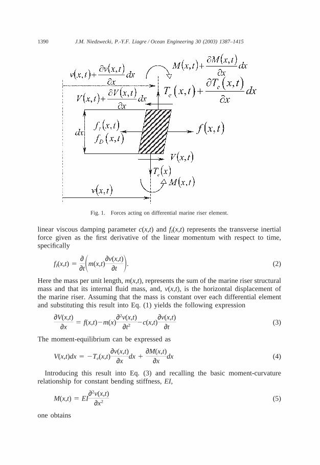
The partial differential equation for the riser motion can be developed from firstprinciples. Because of the symmetry of the marine riser cross-section, the equationsof motions in the two principal vertical planes are identical and can be derivedindependently for each plane. The coupling in the direction of the wave excitationoriginates from relative motion between the response and the excitation. Theresulting non-linear hydrodynamic drag forces are calculated using the modifiedMorison equation with a correction for the variation in free surface elevation as thewaves pass the marine riser. As shown on Fig. 1, the length of the differential elementis dx. At both end of the segment, the internal member forces are shown, and theseinclude the shear, V, the moment, M, and axial forces, Te. The resultant of all theexternal loads f(x,t) and inertia forces fI(x,t) are shown at the midpoint of the segment.

Summing the forces acting on the differential element in the horizontal planeyields

∂V(x,t)∂x

� f(x,t)�fI(x,t)�fD(x,t), (1)

where, fD(x,t) represents the medium (air or water) resistance associated with the


Fig. 1. Forces acting on differential marine riser element.

linear viscous damping parameter c(x,t) and fI(x,t) represents the transverse inertialforce given as the first derivative of the linear momentum with respect to time,specifically

fI(x,t) �∂∂t�m(x,t)

∂v(x,t)∂t �. (2)

Here the mass per unit length, m(x,t), represents the sum of the marine riser structuralmass and that its internal fluid mass, and, v(x,t), is the horizontal displacement ofthe marine riser. Assuming that the mass is constant over each differential elementand substituting this result into Eq. (1) yields the following expression

∂V(x,t)∂x

� f(x,t)�m(x)∂2v(x,t)

∂t2�c(x,t)

∂v(x,t)∂t

(3)

The moment-equilibrium can be expressed as

V(x,t)dx � �Te(x,t)∂v(x,t)

∂xdx �

∂M(x,t)∂x

dx (4)

Introducing this result into Eq. (3) and recalling the basic moment-curvaturerelationship for constant bending stiffness, EI,

M(x,t) � EI∂2v(x,t)

∂x2 (5)

one obtains


EI∂4v(x,t)

∂x4 �Te(x,t)∂2v(x,t)

∂x2 �∂Te(x,t)

∂x∂v(x,t)

∂x� m(x)

∂2v(x,t)∂t2

� c(x,t)∂v(x,t)

∂t(6)

� f(x,t)

As described in McIver and Olson (1981), for most purposes the axial tension canbe computed from the weight per unit length w, assuming that the riser remainsnearly vertical. Each segment of the riser is subjected to an effective tensionTe(x,t) of the form

Te(x,t) � Ttop��L

x

w(e,t)de (7)

where, Ttop, is the applied tension at the top of the riser and, w, is equal to theproduct of the mass per unit length and acceleration of gravity for the elementslocated above the free surface of the waves and the buoyant weight for totally sub-merged elements. In the numerical simulations this problem variable is allowed tovary with position and time in order to address the undulation of the wave freesurface in the wave zone.

Finally, substituting Eq. (7) into Eq. (6) yields

EI∂4v(x,t)

∂x4 � Te(x,t)∂2v(x,t)

∂x2 �w(x,t)∂v(x,t)

∂x� m(x)

∂2v(x,t)∂t2

� c(x,t)∂v(x,t)

∂t(8)

� f(x,t)

This quasi-linear fourth order partial differential equation governs the riser responseto a general dynamic and distributed external excitation f(x,t). Discretization of themariner riser along the spatial coordinate, x, leads to the development of a coupledsystem of governing equations.

2.2. Wave force excitation: classical approach

The primary environmental loading addressed in this study is due to ocean surfacewaves, although it is straightforward to consider ocean currents as well. Because amarine riser is basically a slender body, the in-line wave force can be computedusing the well-known Morison equation that is the sum of the drag and inertia forcecomponents. Also it is assumed that in the sub-sea region near the marine riser, thekinematics of the flow do not change in the incident wave direction. Taking intoaccount the relative motion between the marine riser and the flow-induced kinemat-ics, the drag force per unit length can be expressed as

fD(x,t) � CD(Re(x,t))rwD

2 �u(x,t)�∂v(x,t)

∂t � | u(x,t)�∂v(x,t)

∂t | (9)

where, u(x,t) is taken as the horizontal component of the water particle velocity,


D is the outer marine riser diameter, rw, the water density and, CD, the drag coef-ficient function which is a function of the local Reynolds number Re(x,t). Correspond-ingly, the inertia force per unit length is of the form

fM(x,t) � CM

rwpD2

4∂u(x,t)

∂t�CA

rwpD2

4∂2v(x,t)

∂t2 (10)

where, CM is the inertia coefficient, herein assumed to be constant. The relationshipbetween the inertia coefficient and the hydrodynamic added-mass coefficient is givenas, CM � CA � 1.

Moving the hydrodynamic added-mass, to the left side of governing equationyields

EI∂4v(x,t)

∂x4 � Te(x,t)∂2v(x,t)

∂x2 �w(x,t)∂v(x,t)

∂x� M(x)

∂2v(x,t)∂t2

� c(x,t)∂v(x,t)

∂t(11)

� f(x,t)

where,

M(x) � m(x) � CA

rwpD2

4(12)

and the wave force excitation, f(x,t), per unit length is then

f(x,t) � CM

rwpD2

4∂u(x,t)

∂t� CD(Re(x,t))

rwD2 �u(x,t)�

∂v(x,t)∂t �| u(x,t) (13)

�∂v(x,t)

∂t |The last term in this equation represents the nonlinear drag force due to the relative

motion between the fluid and the structural response, and it acts effectively to reduce,i.e. dampen, the motion response of the marine riser. Often in practice the nonlineardrag force is linearized resulting in the separation of the kinematic contributions.For example, Sarpkaya and Isaacson (1981) consider an approach where the quad-ratic term of the drag force due to the relative fluid velocity is replaced by a linearexpression involving the root mean square value of the relative velocity, sr. Thenintroducing this approximation and combining Eqs. (11) and (13) one obtains

EI∂4v(x,t)

∂x4 � Te(x,t)∂2v(x,t)

∂x2 �w(x,t)∂v(x,t)

∂x(14)

� M(x)∂2v(x,t)

∂t2 � �c(x,t) � CD

rwD2 �8

psr�∂v(x,t)

∂t� fL(x,t),


with the applied loading of the form

fL(x,t) � CM

rwpD2

4∂u(x,t)

∂t� CD

rwD2 �8

psr u(x,t). (15)

Often as a first approximation, the wave damping due to the relative motion can besimplified assuming that sr�su. Other approximations are available in the openliterature such as that proposed by Krolikowsky and Gay (1980) for dealing withwaves and currents.

2.3. Wave force excitation: non-classical approach

As one begins to think about the range of sources for non-linear behavior that arepossible, other approaches to modeling the non-linear response behavior need to beconsidered. In this study, it is suggested that the nonlinear drag force be treated moregenerally following the approach suggested in nonlinear system identification where,

EI∂4v(x,t)

∂x4 � Te(x,t)∂2v(x,t)

∂x2 �w(x,t)∂v(x,t)

∂x� M(x)

∂2v(x,t)∂t2

� c(x,t)∂v(x,t)

∂t(16)

� p(x,x,…,t) � fL(x,t)

where, p(x,x,…,t) can take on classical forms such as the Duffing, Van der Pol orpolynomial types of non-linearities. In this study a general non-linear damping-restoring term based upon the combination of classic Duffing and Van der Pol nonlin-earities is used, specifically,

p(x,x,...,t) � k3 v3(x,t) �c3

3∂v3(x,t)

∂t, (17)

where, k3, is the Duffing coefficient and, c3, is the Van der Pol coefficient. TheDuffing non-linearity acts as an artificial spring with variable positive stiffness,k3(x) v2(x,t), that increases as the displacement, v(x,t), gets larger. Such a springgrows stiffer as the riser differential elements moves away from its equilibrium pos-ition, but it recovers its original value when the segments return to their originalposition. Thus, high-amplitude excursions should oscillate faster than low-amplitudeones, and the sinusoidal shapes should be “pinched in” at their peaks. The Van derPol non-linearity acts as an additional damper. The nature of Eq. (17) will becomemore evident in the derivation of the system identification approach.

2.4. Modeling the wave kinematics

Linear wave theory is adopted as the basis for modeling regular and random wavetrains used in this study. It should be noted that the system identification approachto be presented in the next section is not limited by this assumption, and any wavetheory of choice can be utilized. Here the wave kinematics are modified usingWheeler stretching technique (Wheeler, 1970) to obtain the wave kinematics up to


the actual free surface. It is assumed that the wave scattering due to the wave-riserinteraction is negligible.

A standard random phase approach is taken to describe a uni-directional randomseaway, in particular the random sea surface elevation is assumed of the form

h(t) � �j � 1

Ajcos(wjt � fj), (18)

where, Aj, is the wave component amplitude obtained based upon a particular randomsea model, wj is the corresponding wave frequency and fj is the random phase angleassumed to be uniformly distributed over the interval [0,2p]. Consistent with linearwave theory, the horizontal water particle velocity and acceleration are expressedrespectively as

u(x,t) � �j � 1

Ajwj

cosh(kjx)sinh(kjd)

cos(wjt � fj) (19)

∂u(x,t)∂t

� �j � 1

Ajw2j

cosh(kjx)sinh(kjd)

sin(wjt � fj) (20)

where, kj is the wave number and is related to wj through the linear dispersion relationfor a specified water depth d, as

w2j � gkjtanh(kjd). (21)

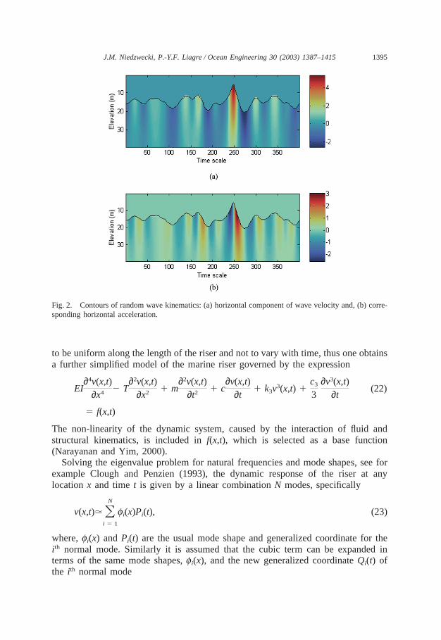
A snapshot of the horizontal wave kinematics, velocity and acceleration, computedfrom the wave elevation recorded during a uni-directional random wave test ispresented in Fig. 2.

3. System identification

System identification procedures for non-linear systems with feedback can be canbe computationally laborious and the procedures can have difficulty in distinguishingbetween linear and non-linear contributions. Bendat (1990) developed an interestingalternative procedure for nonlinear system identification. In his procedure, the rolesof the physical input f(x,t) and physical output v(x,t) are first to be inverted to createa reverse dynamic nonlinear model with no feedback. For this study, an equivalentreverse dynamic two-input/single-output linear model is presented and is based uponthe mathematical marine partial differential equations previously discussed.

3.1. Two-input/single-output reverse dynamic linear model

Consider the partial differential Eq. (16) that governs the riser response for anygiven applied force f(x,t). The physical properties as well as the tension are assumed


Fig. 2. Contours of random wave kinematics: (a) horizontal component of wave velocity and, (b) corre-sponding horizontal acceleration.

to be uniform along the length of the riser and not to vary with time, thus one obtainsa further simplified model of the marine riser governed by the expression

EI∂4v(x,t)

∂x4 � T∂2v(x,t)

∂x2 � m∂2v(x,t)

∂t2� c

∂v(x,t)∂t

� k3v3(x,t) �c3

3∂v3(x,t)

∂t(22)

� f(x,t)

The non-linearity of the dynamic system, caused by the interaction of fluid andstructural kinematics, is included in f(x,t), which is selected as a base function(Narayanan and Yim, 2000).

Solving the eigenvalue problem for natural frequencies and mode shapes, see forexample Clough and Penzien (1993), the dynamic response of the riser at anylocation x and time t is given by a linear combination N modes, specifically

v(x,t)�Ni � 1

fi(x)Pi(t), (23)

where, fi(x) and Pi(t) are the usual mode shape and generalized coordinate for theith normal mode. Similarly it is assumed that the cubic term can be expanded interms of the same mode shapes, fi(x), and the new generalized coordinate Qi(t) ofthe ith normal mode


v3(x,t)Ni � 1

fi(x)Qi(t). (24)

Introducing Eqs. (23) and (24) into Eq. (22) leads to the following expression

Ni � 1

m fi(x)Pi(t) � Ni � 1

c fi(x) Pi(t) � Ni � 1

(EIfivi (x)�Tf�i(x))Pi(t) (25)

� Ni � 1

k3 fi(x) Qi(t) � Ni � 1

c3

3fi(x) Qi(t) � f(x,t)

where, the primes denote space derivatives and the overdots indicate time derivatives.Multiplying each term by fn(x), integrating over the length of the riser and inter-

changing the order of integration and summation yields

Ni � 1

Pi(t)�L

0

m fi(x)fn(x)dx � Ni � 1

Pi(t)�L

0

c fi(x)fn(x)dx � Ni � 1

Pi(t)�L

0

(EIfivi (x)

�Tf�i(x))fn(x)dx � Ni � 1

Qi(t)�L

0

k3 fi(x)fn(x) dx (26)

� Ni � 1

Qi(t)�L

0

c3

3fi(x)fn(x) dx � �

L

0

f(x,t)fn(x) dx

By virtue of the orthogonal properties of the modes, all terms in each of thesummations vanish except the one term for which i � n. Consequently for eachmode n, Eq. (26) can be rewritten as

MnPn(t) � CnPn(t) � KnPn(t) � DnQn(t) � VnQn(t) � Fn(t) (27)

n � 1,2,...,N

where, the generalized mass, damping, stiffness, nonlinear contributions and forceare of the form

Mn � �L

0

m f2n(x)dx (28)

Cn � �L

0

c f2n(x) dx (29)


Kn � �L

0

(EIfivn (x)�Tf�n(x))fn(x)dx (30)

Dn � �L

0

k3 f2n(x)dx (31)

Vn � �L

0

c3

3f2

n(x) dx (32)

Fn(t) � �L

0

f(x,t) fn(x)dx (33)

This set of partial differential equations constitutes the equivalent reverse dynamictwo-input/single-output (TI/SO) linear model from which frequency domain relationscan be derived.

For a upon pin-pin connected beam or string, the vibration shape of the nth modecan be expressed as (Clough and Penzien, 1993)

fn(x) � sin�npxL � (34)

where, L, represents the length of the marine riser. Substituting this result into Eq.(28) through (32) one obtains

Mn �mL2

(35)

Cn �cL2

(36)

Kn �EIL2 �np

L �4

�TL2 �np

L �2

n � 1,2,3,... (37)

Dn �k3L2

(38)

Vn �c3L6

(39)

Finally, since the dynamic response, v(x,t), is known, the generalized coordinatesPn(t) and Qn(t) can be evaluated

Pn(t) �2L�

L

0

v(x,t)sin�npxL �dx (40)


Qn(t) �2L�

L

0

v3(x,t)sin�npxL �dx (41)

In the reverse dynamic model, Fn(t) is the mathematical output, and Pn(t) andQn(t) are the required inputs to the system. The two inputs are computed from thedynamic response of this nonlinear system, and can be non-Gaussian and correlatedto some extent. From knowledge of Pn(t), Qn(t) and Fn(t), without restrictions ontheir probability or spectral properties, the TI/SO linear system can be solved usingthe reverse MI/SO technique to identify the two frequency response functions, fromwhich the system parameters can be recovered. Thus, all that remains in the formu-lation is the development of the frequency domain equations.

3.2. Frequency domain identification

The equivalence between the SI/SO nonlinear system and reverse dynamic TI/SOlinear model featuring a linear sub-system in parallel with a nonlinear sub-systemhas a great significance because the frequency transfer functions between inputsPn(t) and Qn(t) and output Fn(t) can be identified by MI/SO linear technique(Bendat, 1990).

Taking the Fourier Transform of both sides of Eq. (27) gives the frequencydomain relation

En(f)Xn(f) � Fn(f)Yn(f) � Z(f) (42)

where,

Xn(f) � I[Pn(t)] (43)

Yn(f) � I[Qn(t)] (44)

Zn(f) � I[Fn(t)] (45)

and, I[] indicates a Fourier transform.Based on the computation of these three quantities, it is straightforward to compute

the two frequency response functions En(f) and Fn(f)

En(f) � Kn�(2pf)2Mn � j(2pf)Cn (46)

Fn(f) � Dn � j(2pf)Vn (47)

The generalized stiffness, mass and damping for the nth mode of vibration aregiven by

Kn � limf→0

Re(En(f)) (48)

Mn �Kn�Re(En(f))

(2pf)2 (49)

Cn �Im(En(f))

2pf(50)


Dn � Re(Fn(f)) (51)

Vn �Im(Fn(f))

2pf. (52)

Recalling Eqs. (35), (36), (38) and (39), the mass, damping, Duffing and Van derPol terms can be computed from any mode of vibration

m �2L

Mn ∀ n � 1,2,3,... (53)

c �2L

Cn ∀ n � 1,2,3,... (54)

k3 �2L

Dn ∀ n � 1,2,3,... (55)

c3 �6L

Vn ∀ n � 1,2,3,.... (56)

On the other hand, the determination and partition of the flexural stiffness andtension require the value of the generalized stiffness for at least two different modesof vibration. Knowing the generalized stiffness for two different modes of vibrationp and q and recalling Eq. (37), we get a linear system with two equations and twounknowns. Solving for the tension and the flexural, or bending, stiffness are ofthe form

T �q4Kp�p4Kq

L2�q4�pp

L �2

�p4�qpL �2� ∀ p � q (57)

EI �q2Kp�p2Kq

L2�q2�pp

L �4

�p2�qpL �4� ∀ p � q. (58)

4. Numerical examples

A series of numerical examples is presented that explore the adequacy of thenumerical implementation of the formulation to predict response behavior of a marineriser and to demonstrate the applicability of the reverse system identification tech-nique to distributed-parameter systems. The examples utilize numerical simulationsand experimental data as would be expected to be available in design practice.Emphasis is placed on motions in-line with the wave propagation and transversevibrations, set up by vortices shedding from the cylinder, were not considered.


4.1. White noise excitation

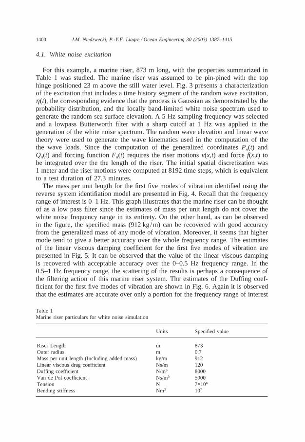
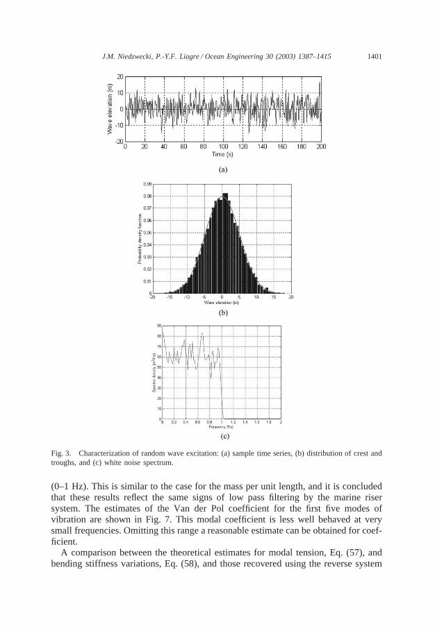
For this example, a marine riser, 873 m long, with the properties summarized inTable 1 was studied. The marine riser was assumed to be pin-pined with the tophinge positioned 23 m above the still water level. Fig. 3 presents a characterizationof the excitation that includes a time history segment of the random wave excitation,h(t), the corresponding evidence that the process is Gaussian as demonstrated by theprobability distribution, and the locally band-limited white noise spectrum used togenerate the random sea surface elevation. A 5 Hz sampling frequency was selectedand a lowpass Butterworth filter with a sharp cutoff at 1 Hz was applied in thegeneration of the white noise spectrum. The random wave elevation and linear wavetheory were used to generate the wave kinematics used in the computation of thethe wave loads. Since the computation of the generalized coordinates Pn(t) andQn(t) and forcing function Fn(t) requires the riser motions v(x,t) and force f(x,t) tobe integrated over the the length of the riser. The initial spatial discretization was1 meter and the riser motions were computed at 8192 time steps, which is equivalentto a test duration of 27.3 minutes.

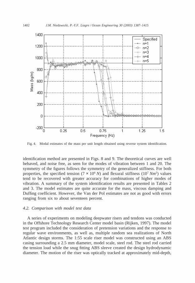
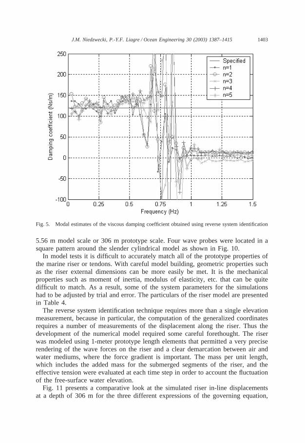
The mass per unit length for the first five modes of vibration identified using thereverse system identifiation model are presented in Fig. 4. Recall that the frequencyrange of interest is 0–1 Hz. This graph illustrates that the marine riser can be thoughtof as a low pass filter since the estimates of mass per unit length do not cover thewhite noise frequency range in its entirety. On the other hand, as can be observedin the figure, the specified mass (912 kg/m) can be recovered with good accuracyfrom the generalized mass of any mode of vibration. Moreover, it seems that highermode tend to give a better accuracy over the whole frequency range. The estimatesof the linear viscous damping coefficient for the first five modes of vibration arepresented in Fig. 5. It can be observed that the value of the linear viscous dampingis recovered with acceptable accuracy over the 0–0.5 Hz frequency range. In the0.5–1 Hz frequency range, the scattering of the results is perhaps a consequence ofthe filtering action of this marine riser system. The estimates of the Duffing coef-ficient for the first five modes of vibration are shown in Fig. 6. Again it is observedthat the estimates are accurate over only a portion for the frequency range of interest

Table 1Marine riser particulars for white noise simulation

Units Specified value

Riser Length m 873Outer radius m 0.7Mass per unit length (Including added mass) kg/m 912Linear viscous drag coefficient Ns/m 120Duffing coefficient N/m3 8000Van de Pol coefficient Ns/m3 5000Tension N 7×106

Bending stiffness Nm2 107


Fig. 3. Characterization of random wave excitation: (a) sample time series, (b) distribution of crest andtroughs, and (c) white noise spectrum.

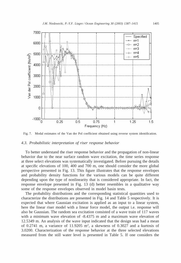
(0–1 Hz). This is similar to the case for the mass per unit length, and it is concludedthat these results reflect the same signs of low pass filtering by the marine risersystem. The estimates of the Van der Pol coefficient for the first five modes ofvibration are shown in Fig. 7. This modal coefficient is less well behaved at verysmall frequencies. Omitting this range a reasonable estimate can be obtained for coef-ficient.

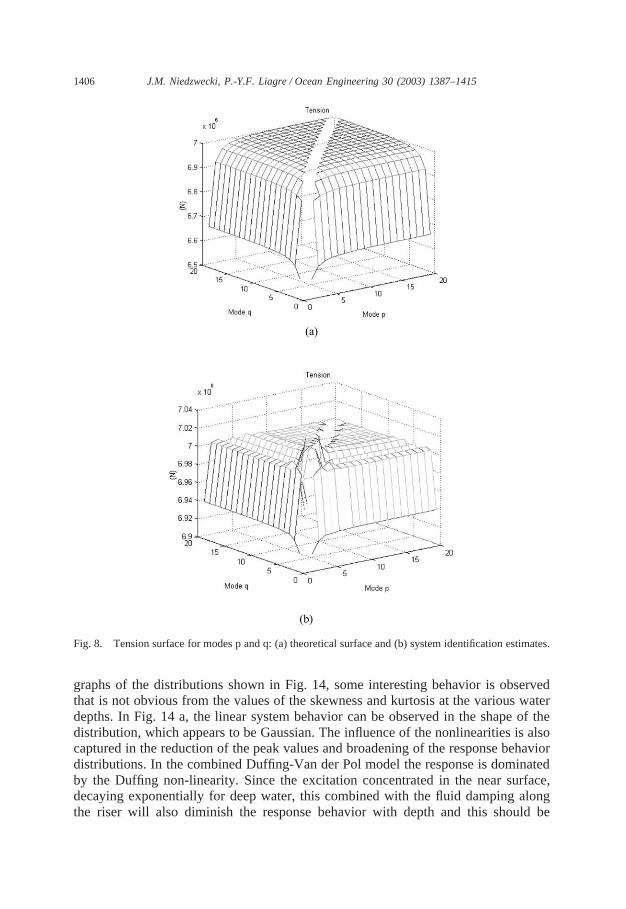
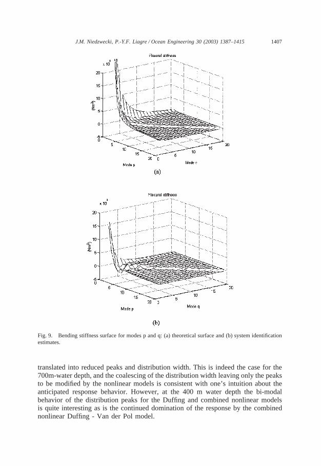
A comparison between the theoretical estimates for modal tension, Eq. (57), andbending stiffness variations, Eq. (58), and those recovered using the reverse system


Fig. 4. Modal estimates of the mass per unit length obtained using reverse system identification.

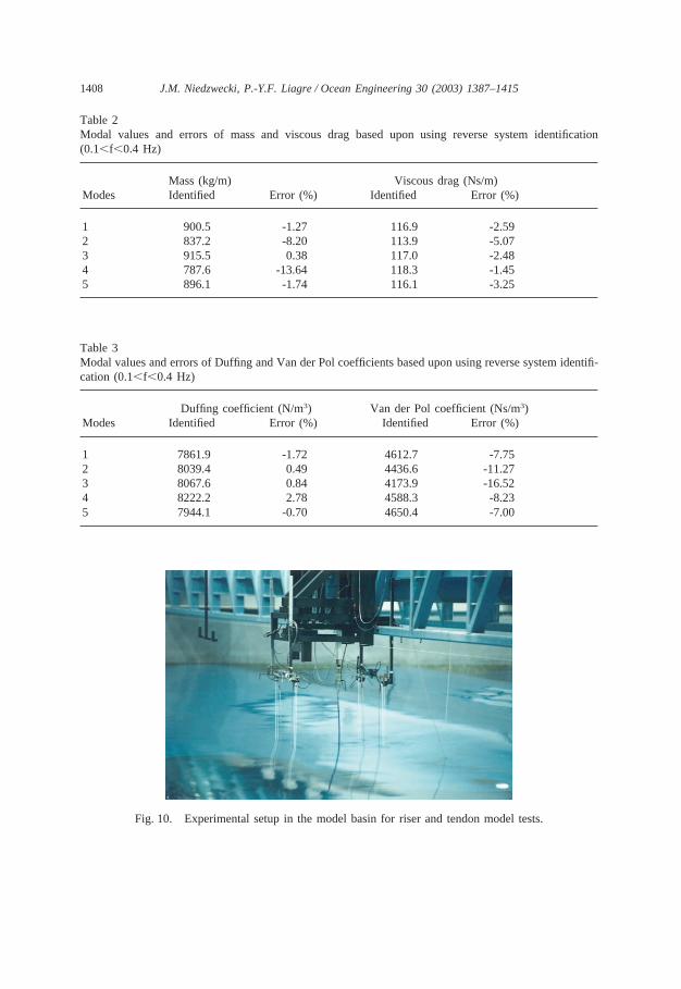
identification method are presented in Figs. 8 and 9. The theoretical curves are wellbehaved, and noise free, as seen for the modes of vibration between 1 and 20. Thesymmetry of the figures follows the symmetry of the generalized stiffness. For bothproperties, the specified tension (7 × 106 N) and flexural stiffness (107 Nm2) valuestend to be recovered with greater accuracy for combinations of higher modes ofvibration. A summary of the system identification results are presented in Tables 2and 3. The model estimates are quite accurate for the mass, viscous damping andDuffing coefficient. However, the Van der Pol estimates are not as good with errorsranging from six to about seventeen percent.

4.2. Comparison with model test data

A series of experiments on modeling deepwater risers and tendons was conductedin the Offshore Technology Research Center model basin (Rijken, 1997). The modeltest program included the consideration of pretension variations and the response toregular wave environments, as well as, multiple random sea realizations of NorthAtlantic design storms. The 1:55 scale riser model was constructed using an ABScasing surrounding a 2.5 mm diameter, model scale, steel rod. The steel rod carriedthe tension load while the snug fitting ABS sleeve created the design hydrodynamicdiameter. The motion of the riser was optically tracked at approximately mid-depth,


Fig. 5. Modal estimates of the viscous damping coefficient obtained using reverse system identification

5.56 m model scale or 306 m prototype scale. Four wave probes were located in asquare pattern around the slender cylindrical model as shown in Fig. 10.

In model tests it is difficult to accurately match all of the prototype properties ofthe marine riser or tendons. With careful model building, geometric properties suchas the riser external dimensions can be more easily be met. It is the mechanicalproperties such as moment of inertia, modulus of elasticity, etc. that can be quitedifficult to match. As a result, some of the system parameters for the simulationshad to be adjusted by trial and error. The particulars of the riser model are presentedin Table 4.

The reverse system identification technique requires more than a single elevationmeasurement, because in particular, the computation of the generalized coordinatesrequires a number of measurements of the displacement along the riser. Thus thedevelopment of the numerical model required some careful forethought. The riserwas modeled using 1-meter prototype length elements that permitted a very preciserendering of the wave forces on the riser and a clear demarcation between air andwater mediums, where the force gradient is important. The mass per unit length,which includes the added mass for the submerged segments of the riser, and theeffective tension were evaluated at each time step in order to account the fluctuationof the free-surface water elevation.

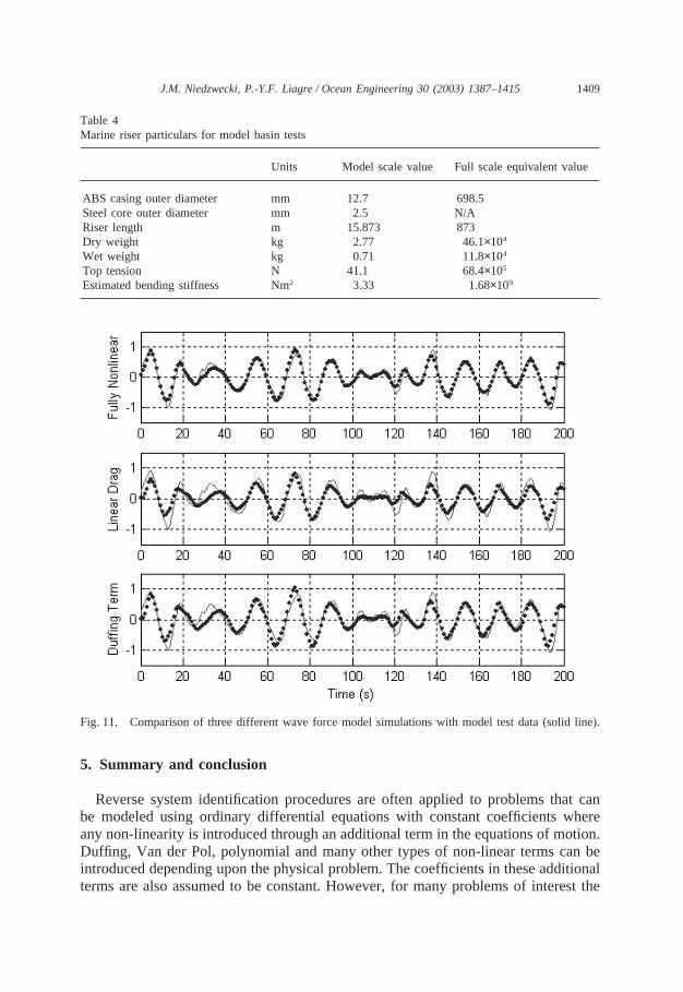
Fig. 11 presents a comparative look at the simulated riser in-line displacementsat a depth of 306 m for the three different expressions of the governing equation,


Fig. 6. Modal estimates of the Duffing coefficient obtained using reverse system identification.

specifically for the fully nonlinear model, the equivalent linear drag force model,the non-linear Duffing coefficient model, and the experimental data. The experi-mental signal (red solid line), over which the simulations are superimposed (bluedots), was extracted from the beginning of a random wave test. It was noticed thatin some cases the experimental response exhibited chaotic behavior a few minutesinto the test. This observed chaotic behavior is an outward sign of vortex-inducedvibrations, which were not modeled in the present study. The simulation using thefully nonlinear governing equation shows very good agreement with the experimentaldata but this success was achieved at the expense of the tedious work of fine-tuningof the parameters. The agreement for the two other simulations can be described asgood and easier to obtain.

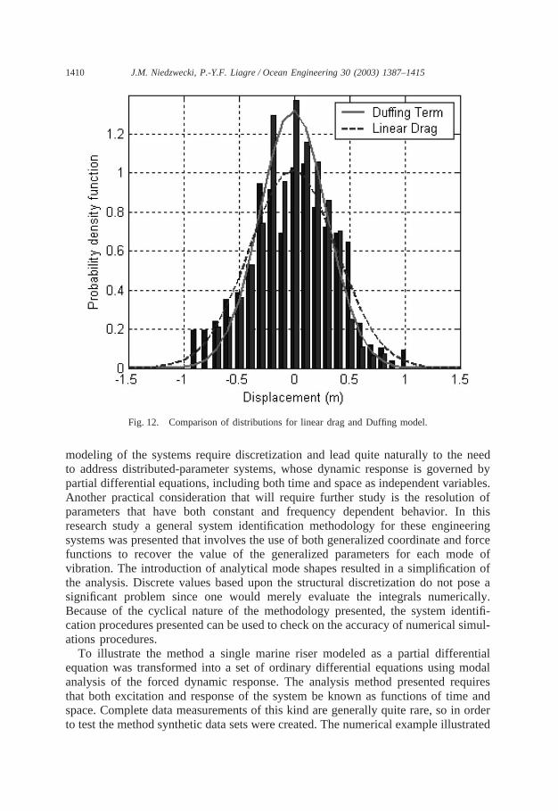
The superposition of histogram and fitted normal distributions of the numericalsimulations for riser displacement at 306 m are presented in Fig. 12, for the lineardrag force model and the Duffing model. The effects of the Duffing coefficient modelare clearly recognizable here in this figure. There are more low amplitude and fewerhigh amplitude oscillations than for the linear drag force simulation. This corrobor-ates the notion that, when including the Duffing coefficient model, high amplitudeexcursions oscillate faster than low amplitude ones, and the sinusoidal shapes are“pinched in” at their peaks. Fine-tuning of the parameters lead to good agreementof the numerical model with the single depth measurement obtained in the labora-tory testing.


Fig. 7. Modal estimates of the Van der Pol coefficient obtained using reverse system identification.

4.3. Probabilistic interpretation of riser response behavior

To better understand the riser response behavior and the propagation of non-linearbehavior due to the near surface random wave excitation, the time series responseat three select elevations was systematically investigated. Before pursuing the detailsat specific elevations of 100, 400 and 700 m, one should consider the more globalperspective presented in Fig. 13. This figure illustrates that the response envelopesand probability density functions for the various models can be quite differentdepending upon the type of nonlinearity that is considered appropriate. In fact, theresponse envelope presented in Fig. 13 (d) better resembles in a qualitative waysome of the response envelopes observed in model basin tests.

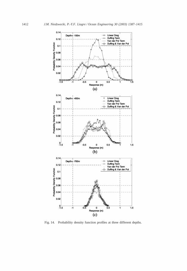
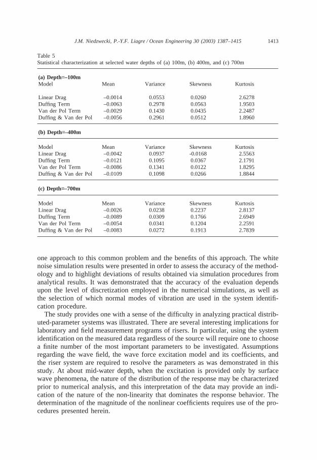
The probability distributions and the corresponding statistical quantities used tocharacterize the distributions are presented in Fig. 14 and Table 5 respectively. It isexpected that where Gaussian excitation is applied as an input to a linear system,here the linear riser model with a linear force model, the output i.e. response willalso be Gaussian. The random sea excitation consisted of a wave train of 117 waveswith a minimum wave elevation of -8.4375 m and a maximum wave elevation of12.5349 m. An analysis of the wave input indicated that the design seas had a meanof 0.2741 m, a variance of 11.9205 m2, a skewness of 0.3027 and a kurtosis of3.0200. Characterization of the response behavior at the three selected elevationsmeasured from the still water level is presented in Table 5. If one considers the


Fig. 8. Tension surface for modes p and q: (a) theoretical surface and (b) system identification estimates.

graphs of the distributions shown in Fig. 14, some interesting behavior is observedthat is not obvious from the values of the skewness and kurtosis at the various waterdepths. In Fig. 14 a, the linear system behavior can be observed in the shape of thedistribution, which appears to be Gaussian. The influence of the nonlinearities is alsocaptured in the reduction of the peak values and broadening of the response behaviordistributions. In the combined Duffing-Van der Pol model the response is dominatedby the Duffing non-linearity. Since the excitation concentrated in the near surface,decaying exponentially for deep water, this combined with the fluid damping alongthe riser will also diminish the response behavior with depth and this should be


Fig. 9. Bending stiffness surface for modes p and q: (a) theoretical surface and (b) system identificationestimates.

translated into reduced peaks and distribution width. This is indeed the case for the700m-water depth, and the coalescing of the distribution width leaving only the peaksto be modified by the nonlinear models is consistent with one’s intuition about theanticipated response behavior. However, at the 400 m water depth the bi-modalbehavior of the distribution peaks for the Duffing and combined nonlinear modelsis quite interesting as is the continued domination of the response by the combinednonlinear Duffing - Van der Pol model.


Table 2Modal values and errors of mass and viscous drag based upon using reverse system identification(0.1�f�0.4 Hz)

Mass (kg/m) Viscous drag (Ns/m)Modes Identified Error (%) Identified Error (%)

1 900.5 -1.27 116.9 -2.592 837.2 -8.20 113.9 -5.073 915.5 0.38 117.0 -2.484 787.6 -13.64 118.3 -1.455 896.1 -1.74 116.1 -3.25

Table 3Modal values and errors of Duffing and Van der Pol coefficients based upon using reverse system identifi-cation (0.1�f�0.4 Hz)

Duffing coefficient (N/m3) Van der Pol coefficient (Ns/m3)Modes Identified Error (%) Identified Error (%)

1 7861.9 -1.72 4612.7 -7.752 8039.4 0.49 4436.6 -11.273 8067.6 0.84 4173.9 -16.524 8222.2 2.78 4588.3 -8.235 7944.1 -0.70 4650.4 -7.00

Fig. 10. Experimental setup in the model basin for riser and tendon model tests.


Table 4Marine riser particulars for model basin tests

Units Model scale value Full scale equivalent value

ABS casing outer diameter mm 12.7 698.5Steel core outer diameter mm 2.5 N/ARiser length m 15.873 873Dry weight kg 2.77 46.1×104

Wet weight kg 0.71 11.8×104

Top tension N 41.1 68.4×105

Estimated bending stiffness Nm2 3.33 1.68×109

Fig. 11. Comparison of three different wave force model simulations with model test data (solid line).

5. Summary and conclusion

Reverse system identification procedures are often applied to problems that canbe modeled using ordinary differential equations with constant coefficients whereany non-linearity is introduced through an additional term in the equations of motion.Duffing, Van der Pol, polynomial and many other types of non-linear terms can beintroduced depending upon the physical problem. The coefficients in these additionalterms are also assumed to be constant. However, for many problems of interest the


Fig. 12. Comparison of distributions for linear drag and Duffing model.

modeling of the systems require discretization and lead quite naturally to the needto address distributed-parameter systems, whose dynamic response is governed bypartial differential equations, including both time and space as independent variables.Another practical consideration that will require further study is the resolution ofparameters that have both constant and frequency dependent behavior. In thisresearch study a general system identification methodology for these engineeringsystems was presented that involves the use of both generalized coordinate and forcefunctions to recover the value of the generalized parameters for each mode ofvibration. The introduction of analytical mode shapes resulted in a simplification ofthe analysis. Discrete values based upon the structural discretization do not pose asignificant problem since one would merely evaluate the integrals numerically.Because of the cyclical nature of the methodology presented, the system identifi-cation procedures presented can be used to check on the accuracy of numerical simul-ations procedures.

To illustrate the method a single marine riser modeled as a partial differentialequation was transformed into a set of ordinary differential equations using modalanalysis of the forced dynamic response. The analysis method presented requiresthat both excitation and response of the system be known as functions of time andspace. Complete data measurements of this kind are generally quite rare, so in orderto test the method synthetic data sets were created. The numerical example illustrated


Fig. 13. Probability density functions for (a) linear drag force, (b) linear drag force with the Duffingnonlinear model included, (c) linear drag force with the Van der Pol nonlinear model included, (d) lineardrag force with the Duffing and Van der Pol nonlinear models included.


Fig. 14. Probability density function profiles at three different depths.


Table 5Statistical characterization at selected water depths of (a) 100m, (b) 400m, and (c) 700m

(a) Depth=–100mModel Mean Variance Skewness Kurtosis

Linear Drag –0.0014 0.0553 0.0260 2.6278Duffing Term –0.0063 0.2978 0.0563 1.9503Van der Pol Term –0.0029 0.1430 0.0435 2.2487Duffing & Van der Pol –0.0056 0.2961 0.0512 1.8960

(b) Depth=–400m

Model Mean Variance Skewness KurtosisLinear Drag –0.0042 0.0937 -0.0168 2.5563Duffing Term –0.0121 0.1095 0.0367 2.1791Van der Pol Term –0.0086 0.1341 0.0122 1.8295Duffing & Van der Pol –0.0109 0.1098 0.0266 1.8844

(c) Depth=–700m

Model Mean Variance Skewness KurtosisLinear Drag –0.0026 0.0238 0.2237 2.8137Duffing Term –0.0089 0.0309 0.1766 2.6949Van der Pol Term –0.0054 0.0341 0.1204 2.2591Duffing & Van der Pol –0.0083 0.0272 0.1913 2.7839

one approach to this common problem and the benefits of this approach. The whitenoise simulation results were presented in order to assess the accuracy of the method-ology and to highlight deviations of results obtained via simulation procedures fromanalytical results. It was demonstrated that the accuracy of the evaluation dependsupon the level of discretization employed in the numerical simulations, as well asthe selection of which normal modes of vibration are used in the system identifi-cation procedure.

The study provides one with a sense of the difficulty in analyzing practical distrib-uted-parameter systems was illustrated. There are several interesting implications forlaboratory and field measurement programs of risers. In particular, using the systemidentification on the measured data regardless of the source will require one to choosea finite number of the most important parameters to be investigated. Assumptionsregarding the wave field, the wave force excitation model and its coefficients, andthe riser system are required to resolve the parameters as was demonstrated in thisstudy. At about mid-water depth, when the excitation is provided only by surfacewave phenomena, the nature of the distribution of the response may be characterizedprior to numerical analysis, and this interpretation of the data may provide an indi-cation of the nature of the non-linearity that dominates the response behavior. Thedetermination of the magnitude of the nonlinear coefficients requires use of the pro-cedures presented herein.


Acknowledgements

The writers gratefully acknowledge the partial financial support of the OffshoreTechnology Research Center and the Minerals Management Service during thisstudy. The first writer also would like to thank the Wofford Cain foundation fortheir support during this study.

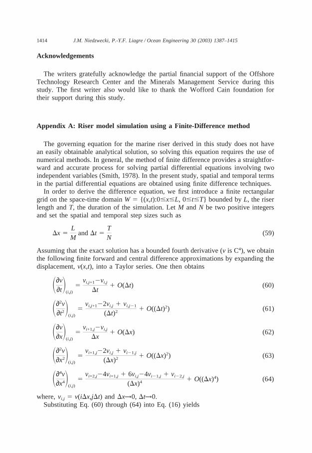
Appendix A: Riser model simulation using a Finite-Difference method

The governing equation for the marine riser derived in this study does not havean easily obtainable analytical solution, so solving this equation requires the use ofnumerical methods. In general, the method of finite difference provides a straightfor-ward and accurate process for solving partial differential equations involving twoindependent variables (Smith, 1978). In the present study, spatial and temporal termsin the partial differential equations are obtained using finite difference techniques.

In order to derive the difference equation, we first introduce a finite rectangulargrid on the space-time domain W � {(x,t):0�x�L, 0�t�T} bounded by L, the riserlength and T, the duration of the simulation. Let M and N be two positive integersand set the spatial and temporal step sizes such as

x �LM

and t �TN

(59)

Assuming that the exact solution has a bounded fourth derivative (v is C4), we obtainthe following finite forward and central difference approximations by expanding thedisplacement, v(x,t), into a Taylor series. One then obtains

�∂v∂t�(i,j)

�vi,j+1�vi,j

t� O(t) (60)

�∂2v∂t2�(i,j)

�vi,j+1�2vi,j � vi,j�1

(t)2 � O((t)2) (61)

�∂v∂x�(i,j)

�vi+1,j�vi,j

x� O(x) (62)

�∂2v∂x2�

(i,j)

�vi+1,j�2vi,j � vi�1,j

(x)2 � O((x)2) (63)

�∂4v∂x4�

(i,j)

�vi+2,j�4vi+1,j � 6vi,j�4vi�1,j � vi�2,j

(x)4 � O((x)4) (64)

where, vi,j � v(ix,jt) and x→0, t→0.Substituting Eq. (60) through (64) into Eq. (16) yields


vi,j+1 � �fL�EIvi+2,j�4vi+1,j � 6vi,j�4vi�1,j � vi�2,j

(x)4 � Ti,j

vi+1,j�2vi,j � vi�1,j

(x)2 � wi,j

vi+1,j�vi,j

x

�Mi,j

�2vi,j � vi,j�1

(t)2 � ci,j

vi,j

t� �c3

i,j

3t�k3i,j�v3

i,j� /� Mi,j

(t)2 �ci,j

t�

c3i,j

3tv2

i,j�. (65)

This implicit finite difference formula for the marine riser allows for the evaluationof the displacement at the specified node at time tj � 1 � (j � 1)t, once the displace-ments at times tj�1 and tj have been determined. The stability of this method dependson the temporal and spatial step sizes.

References

Banks, H.T., Kunisch, K., 1989. Estimation techniques for distribut parameter systems. In: Systems &Control: Foundations & Applications. Vol. 1. Birkhauser, Boston, MA.

Bendat, J.S., 1990. Nonlinear System Analysis and Identification from Random Data. John Wiley & Sons,New York, NY.

Bendat, J.S., 1993. Spectral techniques for nonlinear system analysis and identification. Shock andVibration 1 (1), 21–31.

Bendat, J.S., 1998. Nonlinear Systems Techniques and Applications. John Wiley & Sons, New York, NY.Bendat, J.S., Piersol, A.G., 1993. Engineering Applications of Correlation and Spectral Analysis, second

ed. John Wiley & Sons, New York, NY.Clough, R.W., Penzien, J., 1993. Dynamics of Structures, second ed. McGraw-Hill, Inc, New York, NY.Imai, H., Yun, C.-B., Maruyama, O., Shinozuka, M., 1989. Fundamentals of system identification in

structural dynamics. Probabilistic Engineering Mechanics 4 (4), 162–173.Jones, N.P., Shi, T., Ellis, J.H., Scanlan, R.H., 1995. System identification procedure for system and input

parameters in ambient vibration surveys. Journal of Wind Engineering and Industrial Aerodynamics54/55, 91–99.

Krolikowsky, L.P., Gay, T.A., 1980. An improved linearization technique for frequency domain riseranalysis. Offshore Technology Conference, OTC 3777, pp. 341–353.

McIver, D.B., Olson, R.J., 1981. Riser Effective Tension—Now You See It, Now You Don’ t! ASMEProceedings of the 37th Petroleum Mechanical Engineering Workshop & Conference, pp. 177–187.

Narayanan, S., Yim, S.C.S., 2000. Nonlinear model evaluation via system identification of a mooredstructural system. Proceedings tenth International Offshore and Polar Engineering Conference.

Panneer-Selvam, R., Bhattacharyya, S.K., 2001. Parameter identification of a compliant nonlinear sdofsystem in random ocean waves by reverse MISO method. Ocean Engineering 28, 1199–1223.

Rice, H.J., Fitzpatrick, J.A., 1991. A procedure for the identification of linear and nonlinear multi-degree-of-freedom systems. Journal of Sound and Vibration 149 (3), 397–411.

Rijken, O.R., 1997. Dynamic Response of Marine Risers and Tendons. Ph.D. Dissertation, Departmentof Civil Engineering, Texas A&M University.

Sarpkaya, T., Isaacson, M., 1981. Mechanics of Wave Forces on Offshore Structures. Van NostrandReinhold, New York, NY.

Smith, G.D., 1978. Numerical Solution of Partial Differential Equations: Finite Difference Method. Clar-endon Press, Oxford, England.

Stansby, P.K., Worden, K., Tomlinson, G.R., Billings, S.A., 1992. Improved wave force classificationusing system identification. Applied Ocean Research 14, 107–118.

Wheeler, J.D., 1970. Method for calculating forces produced by irregular waves. Journal of PetroleumTechnology, 359–367.

system identiﬁcation of distributed-parameter marine ... · can be found in the technical book by...

Documents