1

Ambient Noise Levels in the Continental United States

Daniel E. McNamara and Raymond P. Buland

USGS, Golden, CO

manuscript in review: BSSA, September 2003: PREPRINT

Correspondence to:

Daniel E. McNamaraUSGS1711 Illinois St.

Golden, CO 80401(303) 273-8550 VOICE(303) 273-8600 FAXmcnamara@usgs.gov

ABSTRACTWe present a new approach to characterize the background seismic noise across the

continental United States. Using this approach, power spectral density (PSD) is estimatedat broadband seismic stations for frequencies ranging from ~0.01 to 16 Hz. We selected alarge number of one-hour waveform segments during a 3 year period, from 2001 to 2003,from continuous data collected by the United States National Seismograph Network

(USNSN) and the Advanced National Seismic System (ANSS).For each 1 our segment of continuous data, PSD is estimated and smoothed in full

octave averages at 1/8 octave intervals. Powers for each 1/8 period interval were thenaccumulated in one dB power bins. A statistical analysis of power bins yields probabilitydensity functions (PDFs) as a function of noise power for each of the octave bands ateach station and component. There is no need to account for earthquakes since they mapinto a background probability level. A comparison of day and night PDFs and anexamination of artifacts related to station operation and episodic cultural noise allow usto estimate both the overall station quality and the level of earth noise at each site.Percentage points of the PDFs have been derived to form the basis for noise maps of thecontiguous US at body wave frequencies.

The results of our noise analysis are useful for characterizing the performance ofexisting broadband stations, for detecting operational problems, and should be relevant tothe future siting of Advanced National Seismic System (ANSS) backbone stations. Thenoise maps at body wave frequencies should be useful for estimating the magnitudethreshold for the ANSS backbone and regional networks or conversely for optimizing thedistribution of regional network stations.

2

Introduction

The main function of a seismic network, such as the Advanced National Seismic

System (ANSS), is to provide high quality data for earthquake monitoring, source studies

and Earth structure research. The utility of seismic data is greatly increased when noise

levels are reduced. A good quantification and understanding of seismic noise is a first

step at reducing noise levels in seismic data.

We have two main objectives in presenting this study. One, we intend to provide and

document a standard method to calculate ambient seismic background noise. For direct

comparison to the standard low and high noise models (NLNM and NHNM; Peterson,

1993) we employ the algorithm used to develop the Albuquerque Seismological

Laboratory (ASL) NLNM to compute power spectral density functions (PSDs). We also

present a new statistical approach where we compute probability density functions

(PDFs) to evaluate the full range of noise at a given seismic station. Our approach allows

us to estimate noise levels over a broad range of frequencies from 0.01-16 Hz (100-

0.0625s period). Using this new method it is relatively easy to compare seismic noise

characteristics between different networks in different regions.

Two, we will characterize the variation of ambient background seismic noise levels

across the United States as a function of geography, season and time of day. To

accomplish this objective the USNSN, Global Seismic Network (GSN) and regional

seismograph networks (RSN) broadband stations contributed to the NEIC in real-time are

used to characterize the frequency dependent seismic background noise across the US.

Many of these stations will be integrated into the backbone of the ANSS (Figure 1).

Characterizing the frequency dependent noise levels across the US is the first

essential step in quantifying the theoretical performance of seismic networks. Theoretical

studies provide some guidance in designing networks to optimize earthquake locations.

3

However, in the real world, station performance is highly non-uniform and is determined

by considerations of available power, communications, security, and land usage in

addition to seismic coupling and cultural noise.

Data Processing and Power Spectral Density Method

The USNSN, GSN and RSN broadband stations contributed to the NEIC are well

distributed (Figure 1). For this reason they have been used to obtain seismic spectral

information to characterize seismic noise across the US. Our approach differs from

previous noise studies (Peterson, 1993; Stutzman, et al., 2000; Wilson et al., 2002) in that

we make no attempt to screen the continuous waveforms for quiet data. In most noise

studies, body and surface waves from earthquakes, or system transients and instrumental

glitches such as data gaps, clipping, spikes, mass re-centers or calibration pulses are

removed. These signals are included in our processing because they are generally low

probability occurrences that do not contaminate high probability ambient seismic noise

observed in the PDFs (see below for details). In fact, transient signals are often useful for

evaluating station performance. Also, eliminating this event triggering and removal stage

has the benefit of significantly reducing the PSD computation time by simplifying data

pre-processing.

The algorithm used to develop the ASL NLNM and NHNM (Peterson, 1993; Bendat

and Piersol, 1971) is used to calculate PSDs for all stations in this study. The processing

steps are detailed below.

Pre-processing. For our analysis, we parse continuous time series, for each station

component, into one-hour time series segments, overlapping by 50%, and distributed

continuously throughout the day, week, month. Overlapping time series segments are

used to reduce variance in the PSD estimate (Cooley and Tukey, 1965). The PSD pre-

processing of each one-hour time segment consists of several operations. First, in order to

further reduce the variance of the final PSD estimates, each one-hour time series record is

4

divided into 13 segments, overlapping by 75%. Second, to significantly improve the Fast

Fourier Transform (FFT) speed ratio, by reducing the number of operations, the number

of samples in each of the 13 time series segments is truncated to the next lowest power of

two. Third, in order to minimize long-period contamination, the data are transformed to a

zero mean value such that any long period linear trend is removed by the average slope

method. If trends are not eliminated in the data, large distortions can occur in spectral

processing by nullifying the estimation of low frequency spectral quantities. Fourth, to

suppress side lobe leakage in the resulting FFT, a 10% cosine taper is applied to the ends

of each truncated and detrended time series segment. Tapering the time series has the

effect of smoothing the FFT and minimizing the effect of the discontinuity between the

beginning and end of the time series. The time series variance reduction can be quantified

by the ratio of the total power in the raw FFT to the total power in the smoothed filter

(1.142857) and will be used to correct absolute power in the final spectrum (Bendat and

Piersol, 1973).

Power Spectral Density. The standard method for quantifying seismic background

noise is to calculate the noise power spectral density (PSD). The most common method

for estimating the PSD for stationary random seismic data is called the direct Fourier

transform or Cooley-Tukey method (Cooley and Tukey, 1965). The method computes the

PSD via a finite-range fast Fourier transform (FFT) of the original data and is

advantageous for its computational efficiency.

The finite-range Fourier transform of a periodic time series y(t) is given by:

(1)

where Tr = length of time series segment, 215 = 819.2s,

f = frequency.

Y f T y t e dtr

Tri ft( , ) ( )= ∫ −

0

2π

5

For discrete frequency values, fk, the Fourier components are defined as:

(2)

for , fk=k/N∆t when k = 1, 2, …, N-1,

where ∆t = sample interval (0.025s),

N = number of samples in each time-series segment, N= Tr/∆t.

Hence, using the Fourier components defined above, the total power spectral density

estimate is defined as:

(3)

As is apparent from (3), the total power, Pk, is simply the square of the amplitude

spectrum with a normalization factor of 2∆t/N. It is critical to apply this standard

normalization when comparing PSD estimates with the Albuquerque Seismic Laboratory

new low noise model (NLNM) (Peterson, 1993).

At this point the PSD estimate is corrected by a factor of 1.142857 to account for the

10% cosine taper applied earlier in the processing. Finally, the seismometer instrument

response is removed by dividing the PSD estimate by the instrument transfer function to

acceleration, in the frequency domain. For direct comparison to the NLNM, the PSD

estimate is converted into decibels (dB) with respect to acceleration (m/s2)2/Hz.

The PSD process is repeated for each of the 13 separate overlapping time segments

within the one-hour record. The final PSD estimate for the full hour is calculated as the

average of the 13 segment PSDs. Due to segment averaging, the final PSD estimate has a

YY f T

tk

k r= ( , )∆

Pt

NYk k= 2 2∆

6

95% level of confidence that the spectral point lies within –2.14 dB to +2.87 dB of the

estimate (Peterson, 1993).

Limitations. The PSD technique described above provides stable spectra estimates

over a broad range of periods (0.05-100s) however, it suffers from poor time resolution

due to the long transforms (3600s) and requires many hours of data to compile reliable

statistics. For better resolution at shorter periods, a larger number of shorter records

should be analyzed.

Probability Density Functions

To estimate the true variation of noise at a given station we generate seismic noise

probability density functions (PDFs) from thousands of PSDs processed using the

methods discussed in the previous section. In order to adequately sample the PSDs, full

octave averages are taken in 1/8 octave intervals. This procedure reduces the number of

frequencies by a factor of 169. Thus, power is averaged between a short period (high

frequency) corner, Ts, and a long period (low frequency) corner of Tl=2*Ts, with a center

period, Tc, such that Tc=sqrt(Ts*Tl) is the geometric mean period within the octave. The

geometric means are then evenly spaced in log space. The average power for that octave

is stored with the center period of the octave, Tc, for future analysis. Ts is then

incremented by one 1/8 octave such that Ts = Ts*20.125, to compute the average power for

the next period bin. Tl and Tc are recomputed, powers are averaged within the next period

range Ts to Tl, and the process continues until we reach the longest resolvable period

given the time series window length of the original data, roughly Tr/10 (Figure 2). This

process is repeated for every one-hour PSD estimate, resulting in thousands of smooth

PSD estimates for each station-component pair. Powers are then accumulated in 1 dB

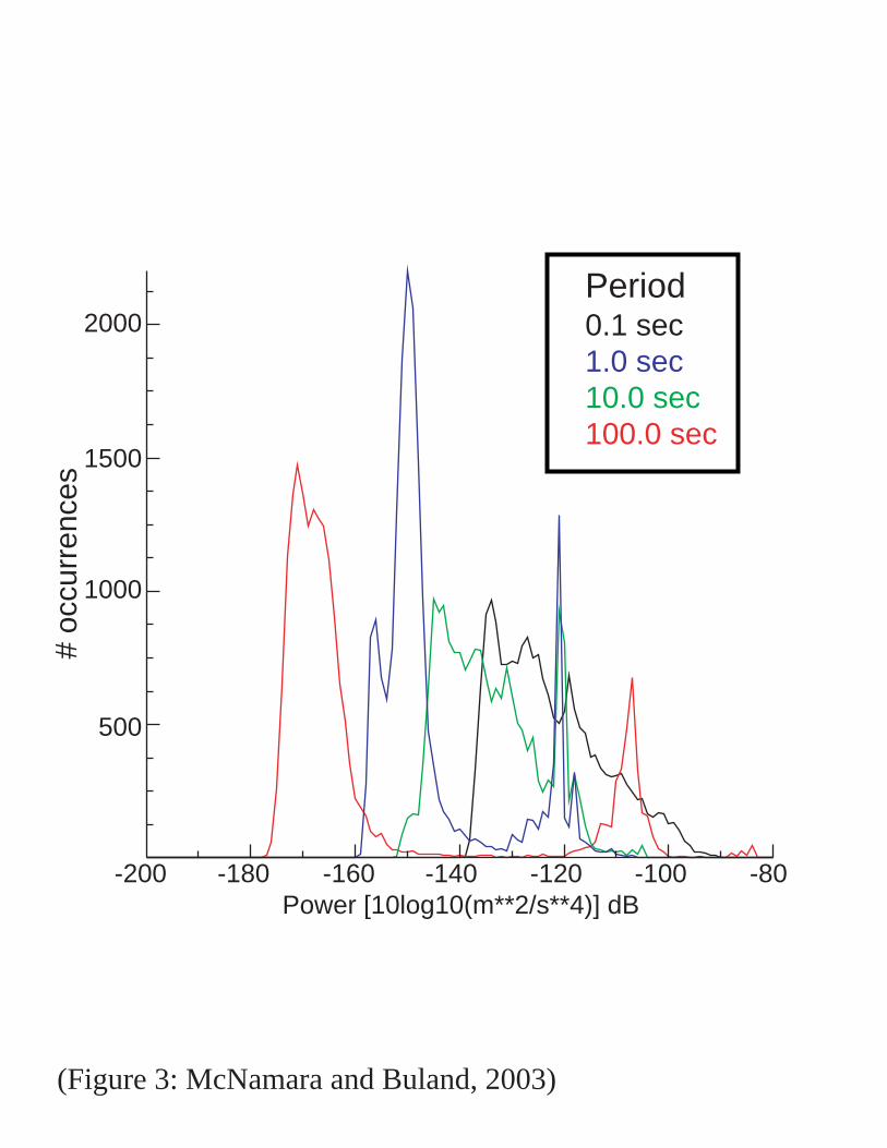
bins to produce frequency distribution plots (histograms), for each period (Figure 3).

Note that each period has a well define low power noise floor while at higher periods we

observe secondary peaks due to system transient and natural noise sources.

7

The probability density function, for a given center period, Tc, can be estimated as:

P(Tc) = NPTc/NTc (4)

where NPTc is the number of spectral estimates that fall into a 1 dB power bin, P, with a

range from –200 to –80 dB, and a center period, Tc. NTc is the total number of spectral

estimates over all powers with a center period, Tc. We then plot the probability of

occurrence of a given power at a particular period for direct comparison to the high and

low noise models (Figure 4). We also compute and plot the minimum, mean, median,

mode, 90th percentile and maximum powers for each period bin. A wealth of seismic

noise information can be obtained from this statistical view of broadband PDFs, as

detailed in the following section (Figure 4).

Characterizing Seismic Noise Sources. Broadband seismograms will always contain

noise. The dominant sources are either from the instrumentation itself or from ambient

Earth vibrations. Normally, seismometer self noise will be well below the seismic noise

so seismologists concentrate on characterizing the latter. For our purposes, we assume

that seismic noise is a stationary process. Specifically, the statistical characteristics of the

seismic noise signal are not strongly time-dependent. The first thing we note about noise

power probability is that the minimum power (red line Figure 4), average (yellow line)

and median (light blue line) closely track the peak noise power probability. This

compression of the observations into a narrow power range suggests to us that each

station can have a characteristic minimum level of background Earth noise. We also note

that the mode (white line) and 90th percentile (green line) are often affected by system

transients such as telemetry drop-outs. The effect of system transients will be discussed

later.

It is interesting to note that the minimum noise levels (red line Figure 4) are generally

very low probability (1-2%) suggesting that the minimum does not represent common

station noise levels. At higher powers, noise power estimates are spread over a wide

8

range of powers at all periods. This region of the PDF is dominated by high power

occurrences of naturally occurring earthquakes, cultural noise, and recording system

transients. Given this, we will detail several sources of seismic noise observed in the

PDFs.

Cultural noise. The most common source of seismic noise is from the actions of

human beings at or near the surface of the Earth. This is often referred to as “cultural

noise” and originates primarily from the coupling of traffic and machinery energy into

the earth. Cultural noise propagates mainly as high-frequency surface waves (>1-10Hz,1-

0.1s) that attenuate within several kilometers in distance and depth. For this reason

cultural noise will generally be significantly reduced in boreholes, deep caves and

tunnels. Cultural noise shows very strong diurnal variations and has characteristic

frequencies depending on the source of the disturbance. For example, automobile traffic

along a dirt road only 20 meters from station AHID, in Auburn Hills Idaho, creates a 30-

35dB increase in power in the10Hz frequency range (Figure 5). This type of cultural

noise is also observable in the PDFs (AHID Figure 4) as a region of low probability at

high frequencies (1-10Hz, 0.1-1s).

Wind, water and geologic noise. Objects move when responding to wind and this

movement, when coupled into the ground can be major source of seismic noise. In

general, wind turbulence around topography irregularities and the coupling of tree motion

to the ground through its roots will generate high frequency noise signals. In addition,

wind acting on large objects such as towers and telephone poles can cause ground tilt that

appears as longer period noise. Additional sources of significant seismic noise may

include running water, surf, volcanic activity or long period tilt due to thermal

instabilities from poor station design. Smearing at long periods may be associated with

this class of noise (Figure 4).

9

Microseisms. There are two dominant peaks in the seismic noise spectrum that are

both widespread and easily recognizable at all broadband seismic stations worldwide.

The lower amplitude, longer period peak (T=10-16s) is known as the single-frequency

peak. It is generated in shallow coastal waters where ocean wave energy is converted

directly into seismic energy either through vertical pressure variations or from the

crashing of surf on shore (Hasselmann, 1963). The higher amplitude, shorter period peak

(T=4-8s), known as the double-frequency peak, is generated by the superposition of

ocean waves of equal period traveling in opposite directions, thus generating standing

gravity waves of half the period of a standard water wave (Longuet-Higgens, 1950). The

standing gravity waves cause perturbations in the water column that propagate to the

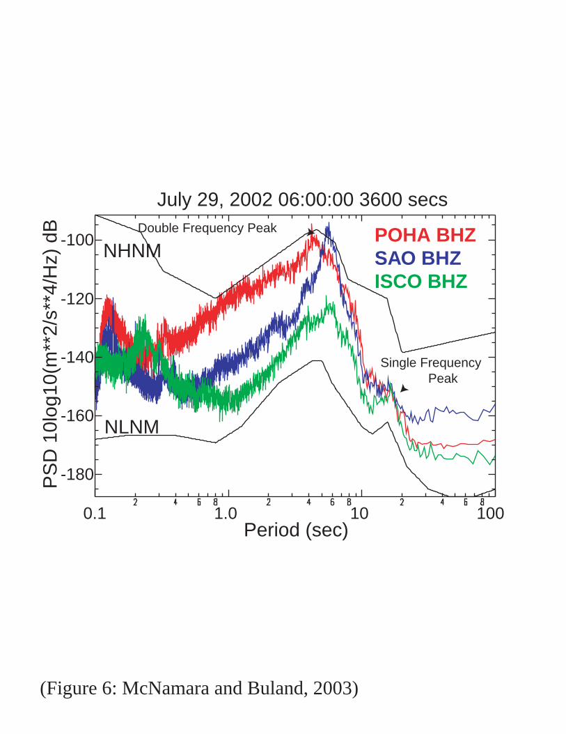
ocean floor and increase significantly during large oceanic storms. An example of

individual PSD estimates, at three unique locations, is shown in Figure 6. Station POHA

is located in the center of the Pacific Ocean on the Island of Hawaii, SAO is <50km from

the coast of northern California and ISCO is located in a mine shaft in the mountains near

Idaho Springs Colorado. Although the microseism noise peak (~4-8s) is readily

observable at all three stations, it is roughly 30db higher at the island station (POHA) and

California (SAO) than in the continental interior (ISCO). We also observe a shift in the

double frequency peak to shorter period for the island station POHA. Microseismic noise

is readily observable in the PDFs. An example for station AHID is seen in figure 4, where

the peak is slightly smeared due to our averaging techniques and to diurnal and/or

seasonal variations.

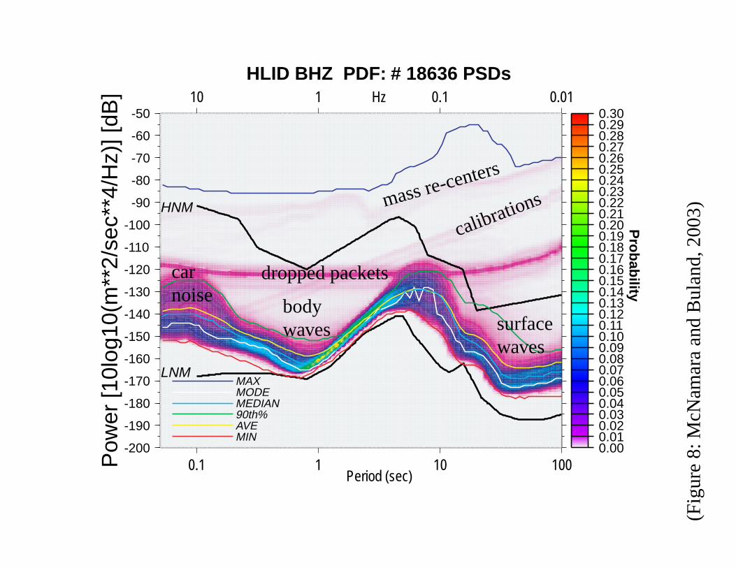
System artifacts in the PDF noise field. Since we make no attempt to screen

waveforms for system transients such as data gaps and sensor glitches, the PDF plots

contain numerous system generated artifacts that can be very useful for network quality

control purposes. We have attempted to determine the source of several coherent, high

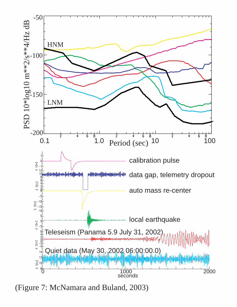
power, low probability noise artifacts in the PDF plots. Figure 7 shows smoothed PSDs

10

and corresponding time series for several system transients and naturally occurring

earthquakes. By comparing with the PDF for HLID BHZ, in Hailey Idaho, (Figure 8),

several artifacts are easily explained and may be useful to the network operator. For

example, data-gaps (due to telemetry drop-outs) and automatic mass re-centers

(necessitated by “drift” in sensor mass position) are easily identifiable in the PSD (Figure

7). When the USNSN satellite telemetry system drops a data packet the data is zero-

filled. Power levels, in the subsequent PSD, reflects the step down from the data to zero.

From the PDF example for HLID we can determine that mass re-centers are

automatically issued less than 1% of the time and that telemetry dropouts are slightly

more common (~1-2%). However, it is easy to imagine that should the probability of

mass re-centering drastically increase the remote network operator could easily diagnose

the problem.

Earthquakes. Our approach differs from many previous noise studies in that we make

no attempt to screen the continuous waveforms to eliminate body and surface waves from

naturally occurring earthquakes. Earthquake signals are included in our processing

because they are generally low probability occurrences even at low power levels (small

magnitude events) (Figure 8). We are interested in the true noise that a given station will

experience, thus we include all signals. For example, including events tells us something

about the probability of teleseismic signals being obscured by small local events as well

as various noise sources. Large teleseismic earthquakes can produce powers above

ambient noise levels across the entire spectrum and are dominated by surface waves

>10s, while small events dominate the short period, <1s (Figure 7). This is also readily

observed in the PDFs as low probability smeared signal at short and long periods (Figure

4 and 8).

11

Diurnal Variations

We analyzed the diurnal variation of seismic noise by accumulating the PSDs in

hourly bins and computing a PDF for each hour of the day over a three-year period at all

stations in our study. We then compute the statistical mode at all periods (Figures 4 and

8), which is the highest probability power level for each hour of the day. Figure 9a is a

plot of the variation in the PDF mode as a function of hour of the day at station BINY,

Binghamton, New York using 19181 hourly PSDs computed from September 2000 to

September 2003. BINY is a surface vault installation in the eastern US and has mode

power variations on the order of 50dB at long periods (50-100s) throughout the day. The

single-frequency microseism peak at ~8s has little variation while in the cultural noise

band, 0.01-1 sec, we observe powers that vary by 15-20dB. This pattern of increased

noise during the daylight working hours is observed at every station, though the

amplitude of the power varies by station and period. For comparison, station ANMO in

Albuquerque, New Mexico (Figure 9b) is sited in a borehole and shows a weaker, ~10dB,

power variation in the cultural noise band, 0.01-1 sec, and virtually nonexistent variation

at longer periods. The difference between these two stations is most likely due to

installation type. Since high frequency cultural noise attenuates rapidly over short

distances, the borehole site ANMO, displays a weaker diurnal variation. Also, the surface

vault at BINY is likely susceptible to daily thermal variations causing the large power

variations at the longest periods (50-100s).

Seasonal Variations

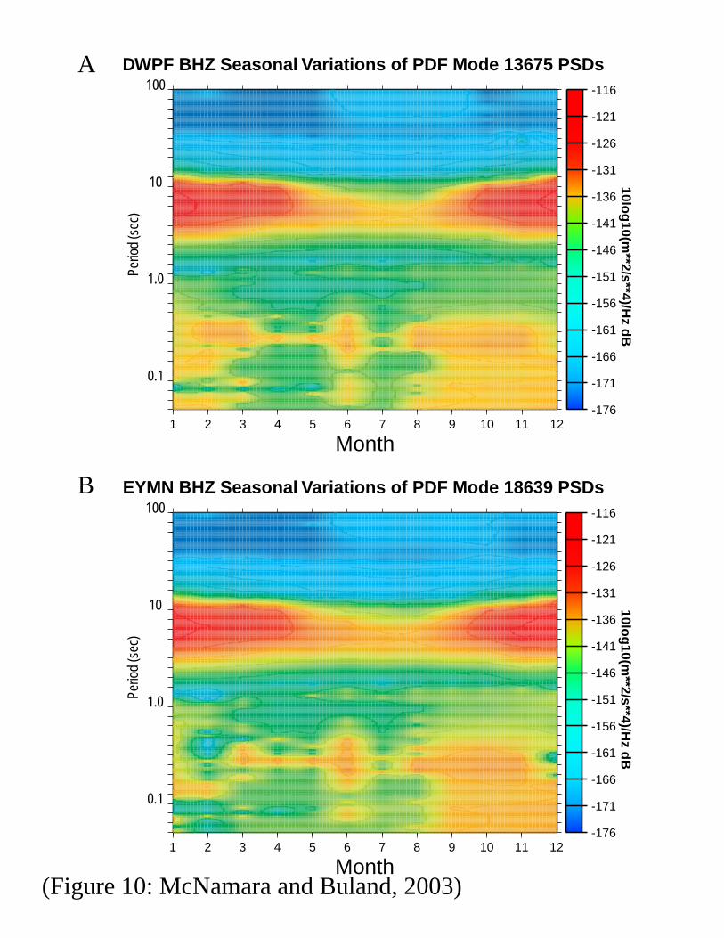
Seasonal variations are computed in the same manner as diurnal variations. We

compute a separate PDF for each month of the year over a three-year period. We then

compute the statistical mode for all periods for each monthly PDF. Figure 10a is a plot of

the seasonal noise variation at station DWPF in Florida. The seasonal variation displays

several interesting patterns. In the microseism band (~8s) there is a strong power increase

12

(~15-20dB) during the winter months and a shift of the microseism peak to slightly

longer periods. These variations are due the increase in the intensity of Atlantic and

Pacific storms during the fall and winter. At longer periods (50-100s) noise increases

during the spring and summer months and decreases during the winter. A number of

mechanisms could contribute to this behavior. Most likely it is due to larger amplitude

daily thermal variations during the warmer months. Short period “cultural” noise appears

to track the microseisms but is much less clear. This pattern is very consistent for all

North American stations. For example, we also observe very similar noise patterns well

into the continental interior at station EYMN in Ely Minnesota (Figure 10b).

Geographic Variations

In order to study the variation of seismic noise as a function of geographic location

we have mapped the average PDF mode for stations in the continental United States. The

mode was chosen since it represents the highest probability power for a given period. We

observe the strongest geographical variations for periods <1s. At these short periods,

cultural noise dominates the signal and the eastern US has significantly higher noise than

the mid-west and western US (Figure 11a). Stations along the eastern coast are as high as

50dB above the NLNM due to their proximity to large population centers. At microseism

periods (Figure 11b) the coastal areas have higher powers relatively to the mid-continent.

At longer periods (Figure 11c) the variation due to geography decreases as individual

station installation type and behavior of the recording system becomes the dominant

factor. In some cases vault design can strongly effect long period response. For example

borehole installations generally produce much lower noise levels at long periods. At all

periods, stations within the continental interior exhibit the lowest noise levels.

Continental stations tend to be above the NLNM by only 10dB or less with the quietest

regions located in the southwestern US.

13

PDF Mode Noise Model

For every station-component, we computed the statistical mode for noise levels from

the PDFs. The PDF mode represents the highest probability noise level for a given station

(Figures 4 and 8). We then computed a new noise model based on the mode levels

(MLNM Figure 12). The MLNM was constructed from the minimum PDF mode noise

values observed per octave and is shown relative to the standard high and low noise of

Peterson (1993) (Figure 12). As is readily observable, the MLNM is on the order of 10-

15 dB higher than the NLNM from 0.01-20s (10-0.05Hz). As we have shown, very few

stations in the US ever reach the low noise levels of the NLNM and the few that do on

occasion (e.g. ISCO, BOZ) have roughly a 1-2% probability of occurrence for a very

narrow band of periods.

Earth noise models have been used as baselines for evaluating seismic site

characteristics since the published high and low seismic background displacement curves

of Brune and Oliver (1959). The NLNM of Peterson (1993) was constructed from

representative quite periods at continental interior stations distributed around the world.

Dominant contributors to the NLNM were LTX, BOSA and ANMO. Today we find that

many of these stations are now surrounded by urban areas with considerably higher noise

levels than was present 20-30 years ago. This is the principle reason that the noise levels

of the NLNM have such low probabilities of occurrence within the continental US. For a

vast majority of stations within the US such low levels of noise are unattainable

suggesting that for routine monitoring purposes our MLNM represents a more realistic

noise threshold. We also expect the MLNM to change with time as population increases

and technology evolves.

Conclusions

We have presented a new method for more realistically evaluating seismic noise

levels at a station based on the power spectral density methods used to generate the

14

NLNM of Peterson (1993). Stations in our analysis exhibit considerable variations in

noise levels as a function of time of day, season, location and installation type. Finally,

we have computed a new MLNM that represents a more realistic noise floor for

earthquake monitoring networks within the United States. The results of our background

noise analysis are useful for characterizing the performance of existing USNSN stations,

for detecting operational problems, and should be relevant to the future siting of ANSS

backbone stations. The noise maps at body wave frequencies should be useful for

estimating the magnitude threshold for the ANSS backbone and regional networks or

conversely for optimizing the distribution of regional network stations.

Acknowledgements

We would like to thank Harold Bolton for detailed discussions and original codes on the

ASL methods used to develop the NLNM. This paper benefited from comments by J. J.

Love and two anonymous reviewers. We also thank Paul Earle for original display of the

PDFs. Maps and PDF plots were creating using the GMT software [Wessel and Smith,

1991].

15

References

Bendat, J.S. and A.G. Piersol (1971). Random data: analysis and measurementprocedures. John wiley and Sons, New York, 407p.

Brune, J.N , and J. Oliver (1959), The seismic noise of the Earth’s surface, Bull. Seism.

Soc. Am., 49, 349-353.Cooley, J.W., and J. W. Tukey (1965), An algorithm for machine calculation of complex

Fourier series, Math. Comp., 19, 297-301.Hasselmann, K. (1963). A statistical analysis of the generation of microsiesms, Rev.

Geophys., 1, 177-209.Longuet-Higgens, M.S. (1950). A theory of the origin of microseisms, Phil. Trans. Roy.

Soc., 243, 1-35.Perterson, Observation and modeling of seismic background noise, U.S. Geol. Surv. Tech.

Rept., 93-322, 1-95, 1993.Stutzman, E., G. Roult, and L. Astiz (2000), Geoscope station noise levels, Bull. Seism.

Soc. Am., 90, 690-701.Wilson, D., J. Leon, R. Aster, J. Ni, J. Schlue, S. Grand, S. Semken, and S. Baldridge

(2002), Broadband seismic background noise at temporary seismic stations observedon a regioanal scale in the southwestern United States, in prep.

Wessel, P. and W. Smith, Free software helps display data, EOS, 72, 445-446, 1991.

16

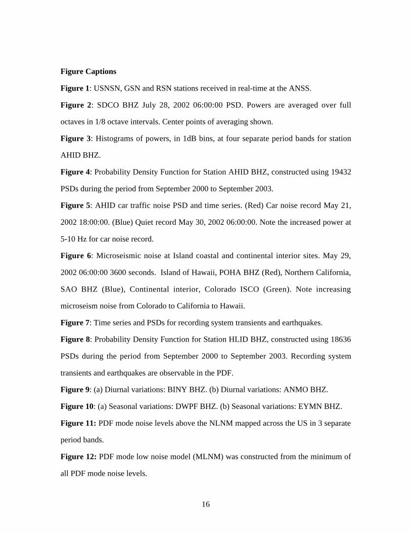
Figure Captions

Figure 1: USNSN, GSN and RSN stations received in real-time at the ANSS.

Figure 2: SDCO BHZ July 28, 2002 06:00:00 PSD. Powers are averaged over full

octaves in 1/8 octave intervals. Center points of averaging shown.

Figure 3: Histograms of powers, in 1dB bins, at four separate period bands for station

AHID BHZ.

Figure 4: Probability Density Function for Station AHID BHZ, constructed using 19432

PSDs during the period from September 2000 to September 2003.

Figure 5: AHID car traffic noise PSD and time series. (Red) Car noise record May 21,

2002 18:00:00. (Blue) Quiet record May 30, 2002 06:00:00. Note the increased power at

5-10 Hz for car noise record.

Figure 6: Microseismic noise at Island coastal and continental interior sites. May 29,

2002 06:00:00 3600 seconds. Island of Hawaii, POHA BHZ (Red), Northern California,

SAO BHZ (Blue), Continental interior, Colorado ISCO (Green). Note increasing

microseism noise from Colorado to California to Hawaii.

Figure 7: Time series and PSDs for recording system transients and earthquakes.

Figure 8: Probability Density Function for Station HLID BHZ, constructed using 18636

PSDs during the period from September 2000 to September 2003. Recording system

transients and earthquakes are observable in the PDF.

Figure 9: (a) Diurnal variations: BINY BHZ. (b) Diurnal variations: ANMO BHZ.

Figure 10: (a) Seasonal variations: DWPF BHZ. (b) Seasonal variations: EYMN BHZ.

Figure 11: PDF mode noise levels above the NLNM mapped across the US in 3 separate

period bands.

Figure 12: PDF mode low noise model (MLNM) was constructed from the minimum of

all PDF mode noise levels.

130ßW

130ßW

120ßW

120ßW

110ßW

110ßW

100ßW

100ßW

90ßW

90ßW

80ßW

80ßW

70ßW

70ßW

60ßW

60ßW

30ßN 30ßN

40ßN 40ßN

50ßN 50ßN

AAMAHID BINY

BLA

BW06

CBKSCBN

DUG

EYMN

GOGA

HAWA

HLID

HWUTISCO

JFWS LBNH

LSCT

LTX

MCWV

MIARMYNC

NEW

NHSC

OCWA

OXF

SDCOTPNV

WMOKWUAZ

WVOR

ANMO

CCM

COR

DWPF

HKT

HRV

PFO

SSPA

TUC

ACSOBMN

BOZ

CMB

DAC

ELKHUMO

ISA

JCT

KNB

LKWY

LRAL

MNV

MSO

MVU

NCB

PLAL

RSSD

TPHWCI

WDC

WVT

USNSN Stations GSN and RSN Stations

(Figure 1: McNamara and Buland, 2003)

Period (sec)

(Figure 2: McNamara and Buland, 2003)

PSD

10*

log1

0 m

**2/

s**4

/Hz

dB

-180

-160

-140

-120

-100

NLNM

NHNM

SDCO BHZ July 28, 2002 06:00:00 PSD

-200 -180 -160 -140 -120 -100 -80Power [10log10(m**2/s**4)] dB

# oc

curr

ence

s

0.1 sec1.0 sec10.0 sec100.0 sec

Period

(Figure 3: McNamara and Buland, 2003)

500

1000

1500

2000

-200

-190

-180

-170

-160

-150

-140

-130

-120

-110

-100

-90

-80

-70

-60

-50P

ower

[10l

og10

(m**

2/se

c**4

/Hz)

] [dB

]

HNM

LNM

AHID BHZ PDF: # 19432 PSDsHz10 1 0.1 0.01

Period (sec)0.1 1 10 100

Pro

bab

ility

MAXMODEMEDIAN90th%AVEMIN

0.000.010.020.030.040.050.060.070.080.090.100.110.120.130.140.150.160.170.180.190.200.210.220.230.240.250.260.270.280.290.30

(Fig

ure

4: M

cNam

ara

and

Bul

and,

200

3)

0.1 1.0 10 100Period (sec)P

SD

10l

og10

(m**

2/s*

*4/H

z) d

BCar Noise

HNM

LNM

-100

-120

-140

-180

-160

0 200 400 600 800 1000seconds

Car Noise

(Figure 5: McNamara and Buland, 2003)

Quiet record

AHID BHZ

May 21, 2002 18:00:00

May 30, 2002 06:00:00

July 29, 2002 06:00:00 3600 secs

POHA BHZSAO BHZISCO BHZ

NHNM

NLNM

0.1 1.0 10 100Period (sec)

PS

D 1

0log

10(m

**2/

s**4

/Hz)

dB

-100

-120

-140

-180

-160

(Figure 6: McNamara and Buland, 2003)

Single Frequency Peak

Double Frequency Peak

(Figure 7: McNamara and Buland, 2003)

Period (sec)

PSD

10*

log1

0 m

**2/

s**4

/Hz

dB

-150

-100

LNM

HNM

-50

0.1 1.0 10 100-200

auto mass re-center

calibration pulse

data gap, telemetry dropout

local earthquake

Teleseism (Panama 5.9 July 31, 2002)

Quiet data (May 30, 2002 06:00:00.0)

0 1000 2000seconds

-200

-190

-180

-170

-160

-150

-140

-130

-120

-110

-100

-90

-80

-70

-60

-50P

ower

[10l

og10

(m**

2/se

c**4

/Hz)

] [dB

]

HNM

LNM

HLID BHZ PDF: # 18636 PSDsHz10 1 0.1 0.01

Period (sec)0.1 1 10 100

Pro

bab

ility

MAXMODEMEDIAN90th%AVEMIN

0.000.010.020.030.040.050.060.070.080.090.100.110.120.130.140.150.160.170.180.190.200.210.220.230.240.250.260.270.280.290.30

mass re-centers

calibrations

dropped packets

bodywaves

carnoise

surfacewaves

(Fig

ure

8: M

cNam

ara

and

Bul

and,

200

3)

0 1 2 3 4 5 6 7 8 9 10 11 12 13 14 15 16 17 18 19 20 21 22 23

GMT hour

-175

-170

-165

-160

-155

-150

-145

-140

-135

-130

-125

-120

-115

-110

-105

BINY BHZ Diurnal Variations of PDF Mode 19181 PSDs

10log

10(m**2/s**4)/H

z dB

100

10

1.0

0.1

Perio

d (s

ec)

(Figure 9: Mcnamara and Buland, 2003)

A

0 1 2 3 4 5 6 7 8 9 10 11 12 13 14 15 16 17 18 19 20 21 22 23

GMT hour

-176

-171

-166

-161

-156

-151

-146

-141

-136

-131

-126

-121

ANMO BHZ Diurnal Variations of PDF Mode 15390 PSDs

10log

10(m**2/s**4)/H

z dB

100

10

1.0

0.1

Perio

d (s

ec)

B

(Figure 10: McNamara and Buland, 2003)

A

B

1 2 3 4 5 6 7 8 9 10 11 12

Month

-176

-171

-166

-161

-156

-151

-146

-141

-136

-131

-126

-121

-116

DWPF BHZ Seasonal Variations of PDF Mode 13675 PSDs

10log

10(m**2/s**4)/H

z dB

100

10

1.0

0.1

Perio

d (s

ec)

1 2 3 4 5 6 7 8 9 10 11 12

Month

-176

-171

-166

-161

-156

-151

-146

-141

-136

-131

-126

-121

-116

EYMN BHZ Seasonal Variations of PDF Mode 18639 PSDs

10log

10(m**2/s**4)/H

z dB

100

10

1.0

0.1

Perio

d (s

ec)

(Figure 11: McNamara and Buland, 2003)

0.125-0.0625 sec Band [8-16 Hz]

120˚W

120˚W

110˚W

110˚W

100˚W

100˚W

90˚W

90˚W

80˚W

80˚W

70˚W

70˚W

60˚W

60˚W

30˚N 30˚N

40˚N 40˚N

50˚N 50˚N

1217222732374247525762

dB

8-4.0 sec Band [0.125-0.25 Hz]

120˚W

120˚W

110˚W

110˚W

100˚W

100˚W

90˚W

90˚W

80˚W

80˚W

70˚W

70˚W

60˚W

60˚W

30˚N 30˚N

40˚N 40˚N

50˚N 50˚N

17

22

27

32

dB

64-32 sec Band [0.015625-0.03125 Hz]

120˚W

120˚W

110˚W

110˚W

100˚W

100˚W

90˚W

90˚W

80˚W

80˚W

70˚W

70˚W

60˚W

60˚W

30˚N 30˚N

40˚N 40˚N

50˚N 50˚N

6111621263136414651566166

dB

A

C

B

(Figure 12: McNamara and Buland, 2003)

Period (sec)

NLNM

NHNM

PS

D 1

0*lo

g10

M**

2/s*

*4/H

z dB

-180

-160

-100

-120

-140

MLNM