eﬀectofschmidtnumberonthevelocity–scalar ...pog/src/schmidt_number_cospec_2005.pdf · 114 p. a....

J. Fluid Mech. (2005), vol. 532, pp. 111–140. c© 2005 Cambridge University Press

doi:10.1017/S0022112005003903 Printed in the United Kingdom

111

Effect of Schmidt number on the velocity–scalarcospectrum in isotropic turbulence with

a mean scalar gradient

By P. A. O’GORMAN AND D. I. PULLINGraduate Aeronautical Laboratories 105-50, California Institute of Technology,

Pasadena, CA 91125, USA

(Received 29 June 2004 and in revised form 14 December 2004)

We consider transport of a passive scalar by an isotropic turbulent velocity field inthe presence of a mean scalar gradient. The velocity–scalar cospectrum measures thedistribution of the mean scalar flux across scales. An inequality is shown to boundthe magnitude of the cospectrum in terms of the shell-summed energy and scalarspectra. At high Schmidt number, this bound limits the possible contribution of thesub-Kolmogorov scales to the scalar flux. At low Schmidt number, we derive anasymptotic result for the cospectrum in the inertial–diffusive range, with a −11/3power law wavenumber dependence, and a comparison is made with results fromlarge-eddy simulation. The sparse direct-interaction perturbation (SDIP) is used tocalculate the cospectrum for a range of Schmidt numbers. The Lumley scaling resultis recovered in the inertial–convective range and the constant of proportionality wascalculated. At high Schmidt numbers, the cospectrum is found to decay exponentiallyin the viscous–convective range, and at low Schmidt numbers, the −11/3 power lawis observed in the inertial–diffusive range. Results are reported for the cospectrumfrom a direct numerical simulation at a Taylor Reynolds number of 265, and acomparison is made at Schmidt number order unity between theory, simulation andexperiment.

1. IntroductionThe problem of turbulent mixing of a passive scalar in the presence of a mean

scalar gradient has been the subject of extensive study, with recent theoretical workfocusing on anomalous scaling of the scalar at small scales (Shraiman & Siggia 2000).As discussed in the review by Warhaft (2000), a number of open issues remain forbehaviour of passive scalar statistics in general, many of them related to the issue oflocal isotropy. The reason for the ubiquity of a mean scalar gradient in studies ofpassive scalar mixing is that the mean gradient acts as a source of scalar variance,allowing a statistical steady state to be reached. The mean gradient makes the scalarfield non-isotropic, and so a mean scalar flux arises. The velocity–scalar cospectrummeasures how this flux is distributed across wavenumbers. If, as is thought, thecospectrum decays faster than the scalar or energy spectra, then this is a measureof the approach to isotropy at the smaller scales. Calculation of the scalar flux is ofpractical importance, and the contribution to the flux from small scales is of relevanceto subgrid modelling and large-eddy simulation (Pullin 2000). Also of interest is theeffect of the Schmidt number, Sc, on the cospectrum, and hence the scalar flux, whereSc is defined as the ratio of viscosity to the scalar diffusivity. The effect of Sc on

112 P. A. O’Gorman and D. I. Pullin

scalar mixing remains a subject of ongoing research, see, for example, the experi-mental work of Miller & Dimotakis (1996), and the simulations of Yeung, Xu &Sreenivasan (2002).

The shell-summed velocity–scalar cospectrum, C(k), is defined so that the meanscalar flux is given by

u1θ =

∫ ∞

0

dk C(k). (1.1)

where θ is the scalar fluctuation, u1 is the component of velocity in the direction of themean scalar gradient, and k is the wavenumber. Shell-summed spectra are sometimesreferred to as three-dimensional spectra and are calculated using an integration overa spherical shell in wavenumber space. Lumley (1967) used a similarity hypothesis topredict the shell-summed cospectrum of the velocity and potential temperature. Forthe case of passive scalar mixing, Lumley’s equation (12) for the cospectrum in theinertial–convective range becomes

C(k) ∼ µε1/3k−7/3, (1.2)

where µ is the mean scalar gradient, and ε is the energy dissipation rate. Mydlarski &Warhaft (1998) measured the one-dimensional velocity–temperature cospectrum in awind tunnel under conditions for which the temperature was a passive scalar. Theyfound a wavenumber dependence of approximately k−2 in the inertial–convectiverange for a Taylor Reynolds numbers, Rλ, of 582; see also Mydlarski (2003). Boset al. (2004) studied the importance of the pressure term in the evolution equation forthe cospectrum and found a k−2 scaling range for the cospectrum using large-eddysimulation (LES). Herr, Wang & Collins (1996) performed an EDQNM calculationof the cospectrum and compared it with direct numerical simulation (DNS) at an Rλ

of 81, although it should be noted that two constants were chosen in the EDQNMcalculation by matching the EDQNM and DNS cospectra. There has also beenwork by Kaneda & Yoshida (2004) and Gargett, Merryfield & Holloway (2003) onthe related problem of the buoyancy flux spectrum in stably stratified turbulence,although here we will exclusively consider the case of a passive scalar.

The velocity–scalar cospectrum was studied by O’Gorman & Pullin (2003) usingthe stretched-spiral vortex model introduced by Lundgren (1982). They found that thecontribution to the cospectrum from the velocity directed parallel to the vortex tubeaxes had a k−5/3 wavenumber-dependence to leading order. The next-order term hada k−7/3 dependence, but its sign depended on the initial conditions. The contributionfrom the velocity in the plane of the vortex structure depended on the choice ofvortex core. In addition, exact relations were derived relating the shell-summed andone-dimensional cospectra, and the quadrature spectrum was shown to be zero.

Here we utilize the sparse direct-interaction perturbation (SDIP) introduced byKida & Goto (1997, hereinafter referred to as KG) with the name Lagrangiandirect-interaction approximation. It is a renormalized closure theory for second-orderturbulent statistics, and applies a similar procedure to Kraichnan’s direct-interactionapproximation (DIA), (Kraichnan 1959), in a Lagrangian framework. The SDIP issimpler than the Lagrangian history DIA of Kraichnan (1965), and yields the sameintegro-differential equations as the Lagrangian renormalized approximation (LRA)obtained earlier by Kaneda (1981). This latter closure has been applied to passivescalar mixing in two and three dimensions, see Kaneda (1986), Gotoh (1989) andGotoh, Nagaki & Kaneda (2000). The SDIP has been used to calculate the energyspectrum (KG), and the scalar spectrum (Goto & Kida 1999), and the resultingscaling exponents were found to be in agreement with classical phenomenology.

Velocity–scalar cospectrum 113

Goto & Kida (2002) applied the SDIP to a simpler model to understand betterthe basis of the approximation. In light of the importance of sparse coupling inthe approximation, the name sparse direct-interaction perturbation was then chosenin place of Lagrangian direct-interaction approximation. There are other two-pointclosures that have been successfully used to calculate turbulent energy and scalarspectra, for example, the local energy-transfer (LET) theory of McComb, Filipiak &Shanmugasundaram (1992). The SDIP is particularly promising for use here sinceGoto & Kida (1999) were able to use it to recover a number of classical scalingresults for the scalar spectrum at different Sc.

In this paper we study the velocity–scalar cospectrum using a combination of theoryand simulation. The cospectrum is defined in § 2, and the form of the cospectrum atdifferent Sc is considered in § 3. An inequality is derived that bounds the magnitudeof the cospectrum, and this is shown to have implications for the cospectrum at highSc. This inequality is an extension of the one-dimensional cross-spectrum inequalityto the shell-summed case, and applied in particular to the velocity–scalar cospectrum.At low Sc, the asymptotic form of the cospectrum in the inertial-diffusive range isderived. The derivation is similar to the argument of Batchelor, Howells & Townsend(1959) for the form of the scalar spectrum in the inertial–diffusive range. The use ofthe SDIP closure to calculate the cospectrum is described in § 4. The Lumley (1967)form is recovered in the inertial–convective range, and the closed equations are solvednumerically for a range of Sc. Finally, in § 5, we report results for the cospectrumfrom both DNS and LES. The DNS was performed at Rλ of 265 and Sc of 0.7, and acomparison is made with theory and experiment at this Sc. The LES was performedat low Sc and agreement is found with the asymptotic form for the cospectrum inthe inertial–diffusive range.

2. The velocity–scalar cospectrumWe consider a passive scalar mixed by an incompressible, statistically homogeneous

and isotropic velocity field, ui(x, t). The scalar is assumed to have a uniformmean scalar gradient, µ, in the 1 direction, so that we can decompose the scalaras µx1 + θ(x, t). The scalar fluctuation θ(x, t) is statistically homogeneous, andaxisymmetric about the x1 axis, but not isotropic. By definition it has zero mean,θ(x, t)= 0, where the overbar indicates an ensemble average.

If we define the velocity–scalar correlation by

Ruiθ (r) = ui(x, t) θ(x + r, t), (2.1)

then the shell-summed cospectrum of the scalar and the velocity component u1 isdefined by

C(k) =1

(2π)3

∫dSk

∫dr Ru1θ (r) exp(−i k · r). (2.2)

Here the∫

dSk integral is a surface integral over a spherical shell in wavenumber

space, and may be written as k2∫ π

0dψk

∫ 2π

0dφk sinψk . The

∫dr integral is a volume

integral over all space. The shell-summed cospectrum has no imaginary part, as maybe seen by performing the shell integral of exp(−i k · r). An important property of thecospectrum is that it integrates to the scalar flux, as given by (1.1). The shell-summedcospectrum is thus a measure of the distribution of the scalar flux across scales.

One-dimensional spectra are often more convenient for experimental measurement,and so we also define a one-dimensional velocity–scalar cospectrum,

C1d(k3) =1

π

∫ ∞

−∞Ru1θ (0, 0, r3) cos(k3r3) dr3, (2.3)


see Bendat & Piersol (1986). The one-dimensional cospectrum also integrates to thescalar flux,

u1θ =

∫ ∞

0

C1d(k3) dk3. (2.4)

It was shown in O’Gorman & Pullin (2003) that only the cospectrum of the scalarand the velocity component in the direction of the mean scalar gradient is non-zero,where this holds for both the shell-summed and one-dimensional cospectra.

3. The cospectrum at small and large Schmidt numberWe consider the effects of Schmidt number on the cospectrum, where the Schmidt

number is defined as the ratio of viscosity to scalar diffusivity, Sc = ν/κ . In latersections we will calculate the cospectrum using turbulence theory and DNS, but wecan use some simpler analysis to limit the possible behaviour of the cospectrum, andin the case of low Sc to predict its asymptotic form.

3.1. The cospectrum inequality

Here we will derive an upper bound for the magnitude of the shell-summed velocity–scalar cospectrum in terms of the energy and scalar spectra. This bound has close tiesto the one-dimensional cross-spectrum inequality and coherence function, discussedin Bendat & Piersol (1986). In effect, we are extending the one-dimensional cross-spectrum inequality to the three-dimensional shell-summed case, and applying it inparticular to the velocity–scalar cospectrum.

It is convenient to use the formulation of the SDIP calculation of § 4, where wefirst work in a periodic box of side L, and then take the limit L → ∞. The velocityfield ui(x, t) can be decomposed as

ui(x, t) =

(2π

L

)3 ∑k

ui(k, t) exp(i k · x), (3.1)

where ki = 2π ni/L, and ni ∈ �. The inverse Fourier transform is given by

ui(k, t) =

(1

2π

)3 ∫d3x ui(x, t) exp(−i k · x), (3.2)

and a similar transformation is defined for the scalar fluctuation, θ(x, t). We thendefine the second-order statistical quantities

Vij (k, t, t) =

(2π

L

)3

ui(k, t) uj (−k, t), (3.3)

Z(k, t, t) =

(2π

L

)3

θ (k, t) θ(−k, t), (3.4)

Wi(k, t, t) =

(2π

L

)3

θ (k, t) ui(−k, t). (3.5)

The double reference to the time t is included to be consistent with the definition ofmore complicated Lagrangian quantities in § 4.

For a given instance in the ensemble, we have

Re(θ (k, t) u1(−k, t)) � |θ(k, t)| |u1(k, t)|, (3.6)


where we have used u(−k, t) = u(k, t)∗. Taking an ensemble average we find that

Re(θ (k, t) u1(−k, t)) � | θ(k, t) | | u1(k, t) | � (| θ (k, t) |2 | u1(k, t) |2)1/2. (3.7)

The second inequality can be derived by considering the expression

(| θ (k, t) | + ξ | u1(k, t) |)2, (3.8)

as a quadratic in the real number ξ , and requiring that it be non-negative.Taking the limit L → ∞, we can relate Vij (k, t, t), Z(k, t, t) and Wi(k, t, t) to power

spectral density functions. The shell-summed energy spectrum, E(k), scalar spectrum,Θ(k), and velocity–scalar cospectrum, C(k), are given by

E(k) = 12

∫dSk Vii(k, t, t), (3.9)

Θ(k) =

∫dSk Z(k, t, t), (3.10)

C(k) =

∫dSk W1(k, t, t), (3.11)

where∫

dSk again denotes a surface integral over a shell in wavenumber space. Wewill now use the fact that the shell-summed cospectrum has no imaginary part. Notingthat the isotropy of the velocity field implies that V 11(k, t, t) =E(k)/(6πk2), and usinginequality (3.7), we deduce that

C(k) �1

k

(∫dSkZ(k, t, t)1/2

)(E(k)

6π

)1/2

. (3.12)

Similarly we can show that inequality (3.12) holds for −C(k), and so it also holds forthe magnitude |C(k)|. The scalar spectrum is anisotropic, and so we cannot performthe surface integral without further knowledge of Z(k, t, t). Nonetheless, we can finda bound in terms of the shell-summed scalar spectrum. Using the Cauchy–Schwartzinequality we have∫

dSkZ(k, t, t)1/211/2 �

(∫dSkZ(k, t, t)

)1/2 (∫dSk

)1/2

= (4π k2 Θ(k))1/2, (3.13)

and so,

|C(k)| �

(2 E(k) Θ(k)

3

)1/2

. (3.14)

A tighter bound might be deduced with more detailed knowledge of the scalaranisotropy.

3.2. Implications of the bound

From (3.14) we see that the magnitude of the cospectrum is bounded by the geometricmean of the scalar and energy spectra multiplied by a constant of order unity. Todiscuss the implications of this, we first briefly review the phenomenology of thescalar spectrum at different Sc.

We assume that the Reynolds number is sufficiently large for an inertial–convective range to exist. We define kP as the wavenumber at the peak of theenergy spectrum or the scalar spectrum, whichever wavenumber is greater. TheKolmogorov wavenumber is defined by kK =(ε/ν3)1/4, the Batchelor wavenumber isgiven by kB =(ε/ν κ2)1/4 = S1/2

c kK , and the Obukhov–Corrsin wavenumber is given by


kC = (ε/κ3)1/4 = S3/4c kK . Then, for wavenumbers in the inertial–convective range, the

scalar spectrum has the form

Θ(k) ∝ εθε−1/3k−5/3, kP � k � min(kK, kC), (3.15)

where εθ is the scalar dissipation and the constant of proportionality is known as theObukhov–Corrsin constant (see Tennekes & Lumley 1974). For large Sc a differentpower law behavior is thought to exist in the viscous–convective range (Batchelor1959),

Θ(k) ∝ εθν1/2ε−1/2k−1, kK � k � kB, Sc 1. (3.16)

For very small Sc, in the inertial–diffusive range,

Θ(k) = 13κ−3Kε2/3εθk

−17/3

(1 +

2κµ2

εθ

), kC � k � kK, Sc � 1, (3.17)

where K is the Kolmogorov constant. We show this in Appendix A, using a directre-derivation of a result of Batchelor et al. (1959), modified for the case of amean scalar gradient. As noted by Chasnov (1991), the effect of the mean scalargradient can be captured by replacing the scalar dissipation with εθ + 2κµ2 in theBatchelor et al. (1959) result. There are other theoretical predictions for the scalarspectrum in the inertial–diffusive range; for example, Gibson (1968) found a k−3

wavenumber dependence. Finally, in the viscous–diffusive range, the scalar spectrumdecays exponentially.

Now consider the velocity–scalar cospectrum for the case of large Sc in the viscous–convective range. According to (3.16), the scalar spectrum has a k−1 wavenumberdependence, whereas the energy spectrum will be decaying exponentially withwavenumber because k kK . Therefore, the bound given by inequality (3.14) willdecay exponentially in this range, and we expect that the cospectrum will also decayexponentially. This would imply that the contribution to the mean scalar flux at lengthscales smaller than the Kolmogorov lengthscale is very small, even if Sc is very large.It should be noted that if the scaling law given by (3.16) is correct, then as Sc → ∞the scalar variance is unbounded; see Dimotakis & Miller (1990) for a discussion ofthis issue.

In contrast, for the case of small Sc in the inertial–diffusive range, the scalarspectrum has a wavenumber dependence of k−17/3 according to (3.17), the energyspectrum has a k−5/3 wavenumber dependence because kP � k � kK , and so the boundgiven by inequality (3.14) has a k−11/3 dependence. Therefore, in this wavenumberrange we cannot exclude either exponential or power law behaviour of the cospectrumbased on the inequality alone. However, we will be able to derive an asymptotic formfor the inertial–diffusive range in the next subsection.

3.3. Asymptotic form in the inertial–diffusive range

We consider the case of low Sc, and wavenumbers in the inertial–diffusive range,kC � k � kK . The advection–diffusion equation for the scalar fluctuation is given by

∂

∂tθ(x, t) + uj (x, t)

∂

∂xj

θ(x, t) = κ∂2

∂xj∂xj

θ(x, t) − µu1(x, t), (3.18)

where we note the gradient forcing term. This can be written in Fourier space as[∂

∂t+ κk2

]θ (k, t) = −µu1(k, t) − i

(2π

L

)3 ∑q

qj uj (k − q, t)θ(q, t). (3.19)


Following the argument of Batchelor et al. (1959), we note that the convolution sumin (3.19) is dominated by wavenumbers q smaller than kC , that is |q| <kC . This isjustified because the scalar spectrum drops off rapidly for higher wavenumbers. Then,assuming that k kC , implies that |k − q| k. We now argue that the time scales ofu1(k, t), uj (k − q, t) and θ(q, t) are much longer that that of θ (k, t). This can be seenin the case of u1(k, t) and uj (k − q, t) by comparing the inertial time scale ε−1/3 k−2/3

with the diffusive time scale κ−1 k−2 and using k kC . Therefore, we can view theright-hand side of (3.19) as a quasi-stationary source term and make a stationarybalance approximation by neglecting the time derivative. Multiplying by u1(−k, t),taking an ensemble average, and using the definition (3.5) of Wi(k, t, t) we find

W1(k, t, t) = − µ

κk2

(2π

L

)3

u1(−k, t)u1(k, t)

− i

κk2

(2π

L

)6 ∑q

qj uj (k − q, t)θ (q, t)u1(−k, t). (3.20)

We have already argued that |q| � |k −q| k, and so we make the further approxima-tion that θ(q, t) is statistically independent of uj (k − q, t) and u1(−k, t). The mean

θ (q, t) is zero, and so

W1(k, t, t) = − µ

κ k2V 11(k, t, t). (3.21)

Taking the limit L → ∞, and using (3.9) and (3.11) to make contact with shell-summedspectra we find

C(k) = − 2µ

3κk2E(k). (3.22)

The wavenumber k is in the inertial range, and so

E(k) = Kε2/3k−5/3, (3.23)

where K is the Kolmogorov constant, with the result

C(k) = −2µK

3κk−11/3ε2/3. (3.24)

Thus the cospectrum has a k−11/3 power law wavenumber-dependence in the inertial–diffusive range. The asymptotic form (3.24) is found to be in agreement with theSDIP result in § 4.4, and with results from LES in § 5.3.

We can also compare our asymptotic result for the cospectrum in the inertial–diffusive range with the bound given by the cospectrum inequality. Substituting (3.23)and (3.17) into (3.14) we find

|C(k)| � 23µKε2/3k−11/3κ−1

(εθ

2κµ2+ 1

)1/2

. (3.25)

Thus the bound exceeds the magnitude of our asymptotic result for the cospectrumby a factor (εθ/(2 κ µ2) + 1)1/2.

In summary, we have used some simple analyses to characterize the behaviour ofthe cospectrum at both large and small Sc. We have mainly discussed inequality (3.14)in the context of the viscous–convective range at large Sc, but it also applies moregenerally. To learn more about the cospectrum in the inertial–convective range, andfor a more detailed characterization of the cospectrum at all scales we turn now tothe SDIP and numerical simulation.


4. SDIP calculationIn this section, we will discuss the use of the SDIP to calculate the velocity–scalar

cospectrum for a range of Sc. We emphasize that we consider a statistically isotropicvelocity field, but a statistically non-isotropic scalar field. Fortunately, we will be ableto use incompressibility of the velocity field and the statistical axisymmetry of thescalar field to describe the cospectrum using a single isotropic function. The resultingSDIP equations are still considerably more complicated than those derived for thescalar spectrum in the isotropic case (Goto & Kida 1999).

The basic formulation is described in § 4.1. The SDIP is applied in Appendix B andthe resulting equations are summarized in § 4.2. In § 4.3, we solve the equations in theinertial–convective range, and in § 4.4 we find the asymptotic solution in the limit oflow Sc. Lastly, in § 4.5, we solve the equations numerically for a range of Sc.

4.1. Basic formulation

The notation we use is consistent with that of Goto & Kida (1999). A more detailedaccount of some of the basic equations can be found in Section II of that paper,although it should be noted that they deal with a statistically isotropic scalar fieldwithout a mean gradient.

The velocity field evolves according to the Navier–Stokes equations,

∂

∂tui(x, t) + uj (x, t)

∂

∂xj

ui(x, t) = − ∂

∂xi

π(x, t) + ν∂2

∂xj∂xj

ui(x, t), (4.1)

where π(x, t) is the pressure–density ratio, and the continuity condition,

∂

∂xi

ui(x, t) = 0. (4.2)

The scalar fluctuation evolves according to the advection–diffusion equation given by(3.18). It is convenient to make use of a Lagrangian position function, ψ(x, t |x ′, t ′),defined by

ψ(x, t |x′, t ′) = δ3(x − y(t |x ′, t ′)), (4.3)

where a fluid element that is located at x ′ at time t ′, is located at y(t |x ′, t ′) at timet � t ′. The Lagrangian position function evolves according to

∂

∂tψ(x, t |x ′, t ′) + uj (x, t)

∂

∂xj

ψ(x, t |x ′, t ′) = 0 (4.4)

with initial condition

ψ(x, t |x ′, t) = δ3(x − x ′). (4.5)

We can then define Lagrangian velocity and scalar fields as

vi(t |x, t ′) =

∫d3x ′ui(x ′, t) ψ(x ′, t |x, t ′), (4.6)

and

θ (L)(t |x, t ′) =

∫d3x ′θ(x ′, t)ψ(x ′, t |x, t ′). (4.7)

The Lagrangian velocity autocorrelation function is given by

Vij (r, t, t ′) = vi(t |x + r, t ′)uj (x, t ′). (4.8)


We wish to calculate the velocity–scalar cospectrum, and so define Lagrangian cross-correlation functions,

Wi(r, t, t ′) = θ (L)(t |x + r, t ′)ui(x, t ′), (4.9)

and

Yi(r, t, t ′) = vi(t |x + r, t ′)θ(x, t ′). (4.10)

The SDIP is formulated in Fourier space by first assuming that the flow is in aperiodic box of side L. The velocity field ui(x, t) can then be decomposed as in (3.1),and the inverse Fourier transform is given by (3.2). Similar transforms are defined forthe other variables. The limit L → ∞ is taken at a later stage. The Fourier transformsof the two-point statistics are given by

V ij (k, t, t ′) =

(2π

L

)3

vi(t |k, t ′)uj (−k, t ′), (4.11)

Wi(k, t, t ′) =

(2π

L

)3

θ (L)(t |k, t ′)ui(−k, t ′), (4.12)

Yi(k, t, t ′) =

(2π

L

)3

vi(t |k, t ′)θ (−k, t ′). (4.13)

It is often more convenient to work with incompressible projections of V ij (k, t, t ′)

and Y i(k, t, t ′), and so we define

Qij (k, t, t ′) = P im(k)V mj (k, t, t ′), (4.14)

Xi(k, t, t ′) = P im(k)Y m(k, t, t ′), (4.15)

where P ij (k) = δij − kikj/k2. After taking the limit L → ∞ we can relate V ii(k, t, t)

to the shell-summed energy spectrum, E(k), and W 1(k, t, t) to the shell-summedvelocity–scalar cospectrum, C(k), see (3.9) and (3.11), respectively. The shell-summedcospectrum can also be related to Y by noting that W 1(k, t, t) = Y 1(−k, t, t).

4.2. Closed equations

The application of the SDIP closure is given in Appendix B. Here, we will summarizethe resulting equations for the case of an isotropic velocity field and a scalar with amean gradient in the ‘1’ direction. We also assume statistical stationarity. With theseassumptions it is shown in Appendix B that we can write

Qij (k, t, t ′) = 12P ij (k)Q†(k, t − t ′), (4.16)

and

Wi(k, t, t ′) = P i1(k)µW †(k, t − t ′), (4.17)

for some functions Q†(k, t − t ′) and W †(k, t − t ′).The closed SDIP equations are then given by

W †(k, t) =

(− 1

2

∫ t

0

Q†(k, t ′) exp[κk2t ′] dt ′ + W †(k, 0)

)exp[−κk2 t], (4.18)

and

2k2(ν + κ)W †(k, 0) + Q†(k, 0) = 12

∫ ∫�k

dpdqπpq

k

σ (k, p, q)

q2

∫ ∞

0

dtM(k, p, q, t),

(4.19)


where

M(k, p, q, t) = (k2 − q2)(k2 − p2 + q2)Q†(k, t)W †(q, t)Q†(p, t)Q†(p, 0)−1

+ ((p2 − q2)2 − k2(p2 − 3q2))Q†(p, t)W †(q, t)Q†(k, t)Q†(k, 0)−1

+ exp[−κq2t]Q†(k, t)Q†(p, t)q2(−4k2W †(k, 0)Q†(k, 0)−1

− (k2 + p2 − q2)W †(p, 0)Q†(p, 0)−1) + (2p2(q2 + k2 − p2)

− 4q2k2)Q†(p, t)W †(k, t)Q†(q, t)Q†(q, 0)−1 + exp[−κk2t]((p2 − q2)2

− k2(p2 − 3q2))Q†(p, t)W †(q, 0)Q†(q, t)Q†(q, 0)−1, (4.20)

and

σ (k, p, q) =(k + p + q)(k + p − q)(k − p + q)(−k + p + q)

4 p2 k2. (4.21)

The wavenumber integral is given by∫ ∫�k

dpdq =

∫ ∞

0

dp

∫ k+p

|k−p|dq.

The linear integral equation (4.19), together with (4.18), are sufficient to determineW †(k, 0) when Q†(k, t) has been specified.

4.3. Inertial–convective range

Here we will solve (4.18) and (4.19) for W †(k, 0) in the inertial–convective range,that is in the wavenumber range where viscosity and diffusivity are unimportant.We introduce a non-dimensional wavenumber k = k/kK , and a non-dimensional timeτ = tε1/3k2/3, where kK = (ε/ν3)1/4 is the Kolmogorov wavenumber. It was shown inKG that according to the SDIP, the velocity correlation function Q†(k, t) can bewritten as

Q†(k, t) =1

2πKε2/3k−11/3Q(k, τ ), (4.22)

where K = 1.722 is the Kolmogorov constant. In particular, in the inertial range wehave

Q†(k, t) =1

2πKε2/3k−11/3Q(0, τ ). (4.23)

Assuming we are in the inertial–convective range means that we can effectively set ν

and κ to zero in (4.18), (4.19) and (4.20). Thus, there are no characteristic scales, andwe can look for solutions of the form

W †(k, 0) = − 1

2πγ ε1/3k−13/3, (4.24)

where γ is a constant to be determined. Then, by (4.18),

W †(k, t) = W †(k, 0)

(1 +

K

2γR

(0, k2/3ε1/3t

)), (4.25)

where R(k, τ ) is given by

R(k, τ ) = exp[−k4/3τ/Sc

] ∫ τ

0

dτ ′Q(k, τ ′) exp[k4/3τ ′/Sc

]. (4.26)

Note that we will use R(k, τ ) for non-zero k in § 4.4.


Substituting (4.23), (4.24) and (4.25), into (4.19), the powers of k factor out, and wefind after some changes of integration variables that

γ = −1

a(1 + bK), (4.27)

where

a = 14

∫ ∫�1

dpdqσ (1, p, q)

q2pq

[(1 − q2)(1 − p2 + q2)q−13/3f (p)

− (1 + p2 − q2)q2p−13/3f (p) − 4q2p−11/3f (p) + ((p2 − q2)2

− (p2 − 3q2))p−11/3q−13/3f (p) + (2p2(q2 + 1 − p2) − 4q2)p−13/3f

(q

p

)

+ ((p2 − q2)2 − (p2 − 3q2))p−13/3q−13/3f

(q

p

) ], (4.28)

b = 18

∫ ∫�1

dpdqσ (1, p, q)

q2pq

[(1 − q2)(1 − p2 + q2)q−13/3g(p, q)

+ ((p2 − q2)2 − (p2 − 3q2))p−11/3q−13/3g(p, q)

+ (2p2(q2 + 1 − p2) − 4q2)p−11/3h(p, q)], (4.29)

and

f (p) =

∫ ∞

0

dτQ(0, τ )Q(0, p2/3τ

), (4.30)

g(p, q) =

∫ ∞

0

dτQ(0, τ )Q(0, p2/3τ

)R

(0, q2/3τ

), (4.31)

h(p, q) =

∫ ∞

0

dτQ(0, p2/3τ

)Q

(0, q2/3τ

)R(0, τ ). (4.32)

Several of the terms in (4.28) and (4.29) contain non-integrable singularities, but thesecan be shown to cancel each other to give finite values for a and b. It is such cancella-tions of singularities that allow Lagrangian reformulations of the DIA to give an en-ergy spectrum with a k−5/3 wavenumber dependence in the inertial range; see McComb(1990) and Leslie (1973). To evaluate the constant γ we must specify Q(0, τ ). Compar-ing with KG we find that their function Q†(τ ) is given by Q†(τ ) = Q(0, K−1/2 τ ), andwe repeated their numerical calculation to determine Q†(τ ). Performing the integrals in(4.28) and (4.29), we found a = −0.44 and b = 0.070, implying γ = 2.6. The numericalintegrations in this paper were carried out using adaptive Gauss–Konrod integrationroutines from the GNU Scientific Library (Galassi et al. 2001).

The shell-summed cospectrum can be evaluated using (3.11) and (4.17) to give

C(k) = − 43µγ ε1/3k−7/3. (4.33)

Thus, the SDIP agrees with the Lumley (1967) form for the cospectrum in theinertial–convective range (1.2), and also gives the constant of proportionality.


4.4. The SDIP equations at low Sc

Here we will derive the asymptotic form of the SDIP equations for Sc � 1. We willthen compare it with the non-SDIP asymptotic result of § 3. It will be useful, both hereand when obtaining numerical solutions, to write (4.18) and (4.19) in non-dimensionalform. We introduce the non-dimensional function W (k) defined by

W †(k, 0) = − 1

2πγ ε1/3k−13/3W (k). (4.34)

The limit k → 0 represents the inertial–convective range, and so from (4.24) we findthat W (0) = 1. Some changes of integration variables result in the following linearintegral equation for W (k),

N1(k)W (k) + N2(k) +

∫ ∞

0

dqN3(k, q)W (kq) = 0, (4.35)

where

N1(k) = 2k4/3

(1 +

1

Sc

)γ

− Kγ

∫ ∞

0

dq

∫ 1+q

|1−q|dp

∫ ∞

0

dτp

qσ (1, p, q)p−11/3Q

(kp, τp2/3

)×

[− exp

[− k4/3q2τ/Sc

]q2Q(k, τ )Q(k, 0)−1

+ exp[−k4/3τ/Sc

](12p2(q2 + 1 − p2) − q2

)Q

(kq, τq2/3

)Q(kq, 0)−1

], (4.36)

N2(k) = −KQ(k, 0) − 18K2

∫ ∞

0

dq

∫ 1+q

|1−q|dp

∫ ∞

0

dτp

qσ (1, p, q)Q

(kp, τp2/3

)×

[(1 − q2)(1 − p2 + q2)Q(k, τ )Q

(kp, 0)−1R(kq, τq2/3

)q−13/3

+ ((p2 − q2)2 − p2 + 3q2)Q(k, τ )Q(k, 0)−1R(kq, τq2/3

)p−11/3q−13/3

+ (2p2(q2 + 1 − p2) − 4q2)Q(kq, τq2/3

)Q(kq, 0)−1R(k, τ )p−11/3

], (4.37)

N3(k, q) = − 14γKq−13/3

∫ 1+q

|1−q|dp

∫ ∞

0

dτp

qσ (1, p, q)

×[(1 − q2)(1 − p2 + q2)Q(k, τ )Q

(kp, τp2/3

)Q(kp, 0)−1 exp

[− k4/3q2τ/Sc

]+((p2 − q2)2 − p2 + 3q2)p−11/3Q

(kp, τp2/3

)× (Q(k, τ )Q(k, 0)−1 exp

[− k4/3q2τ/Sc

]+Q

(kq, τq2/3

)Q(kq, 0)−1 exp

[− k4/3τ/Sc

])− p2(1+q2 −p2)Q(k, τ )Q

(kq, τq2/3

)Q(kq, 0)−1exp

[−k4/3p2τ/Sc

]]. (4.38)

Note that R(k, τ ) is defined by (4.26), and that we have effectively combined (4.18)and (4.19) into one equation for W (k).

For clarity of analysis when taking the small Sc limit we follow Goto & Kida (1999)by introducing the rescaled quantities k = ksS

αc and W (k) = Ws(ks)S

βc , where ks and

Ws are assumed to be order unity as Sc → 0. The Kolmogorov wavenumber and theObukhov–Corrsin wavenumber then correspond to α = 0 and α = 3/4, respectively.We wish to consider wavenumbers k kC and so α < 3/4. Typical exponential factorsinvolving Sc are rewritten as

exp[−k4/3τ/Sc

]= exp

[−k4/3

s τS4α/3−1c

] 0, (4.39)


because 4α/3 − 1 < 0. Therefore in (4.35) we can neglect N3, and N1 is approximatedby

N1 2k4/3s S4α/3−1

c γ . (4.40)

Care must be taken with the function R(k, τ ), which is written using the rescaledquantities as

R(k, τ ) =

∫ τ

0

dτ ′Q(k, τ ′) exp[

− k4/3s S4α/3−1

c (τ − τ ′)]. (4.41)

Noting that τ � τ ′ we have

N2 −KQ(ksS

αc , 0

). (4.42)

The relevant scaling for Ws(ks) is then β = −4α/3 + 1, with the result

Ws(ks) =KQ

(ksS

αc , 0

)2k

4/3s γ

. (4.43)

Returning to unscaled variables, we have

W (k) =KQ(k, 0)Sc

2k4/3γ, k kC. (4.44)

The corresponding form for the shell-summed cospectrum is

C(k) = − 2µ

3κk2E(k), k kC, (4.45)

and for kC � k � kK we recover (3.24). Therefore the SDIP equation is consistent withthe asymptotic result of § 3.3 for the inertial–diffusive range that was derived usingthe simpler Batchelor et al. (1959) type analysis. The SDIP asymptotic form (4.45) ismore general since it applies in the viscous–diffusive range also. The SDIP equationsare solved numerically in § 4.5 and the asymptotic form (4.45) is verified.

4.5. Numerical solution

Here we will solve (4.35) numerically for a range of values of Sc. Equation (4.35)is an inhomogeneous Fredholm integral equation of the second kind. As written,the integrals giving N1(k)W (k) and

∫ ∞0

dqN3(k, q)W (k q) do not converge, becauseof a non-integrable singularity as (p → 0, q → 1). These singularities do cancel eachother, but involve the unknown function W (k) in a way that makes adding andsubtracting the singularity difficult. Therefore, the method of solution chosen was touse a Newton–Raphson solver. This simplifies the problem because calculation of theresiduals requires finding the left-hand side of the equation, but not each individualterm. Although the equation is linear, in practice two iterations were required forgood accuracy.

The q integration was performed using a Gauss–Jacobi rule, and the p and τ

integrations were performed using adaptive Gauss–Konrod integration. The Jacobianrequired for the Newton–Raphson solver was calculated using finite differences, andinterpolations were performed using cubic and bicubic spline interpolation for W (k)and Q(k, τ ), respectively.

The results were found to be converged when the integral equation was evaluatedat twenty points, and when for the q integration the integrand was evaluated attwenty-four points. The integral equation was evaluated at the same points as whereW (k) was stored, but these points were chosen to be different from the quadrature


10–2 10–1 100

10–2

10–1

100

101(a)

–C(k

) µ

–1 ε

1/4 ν

–7/4

(k/

k K)7/

3

k/kK

10–4 10–3 10–2 10–1 100

k/kK

10–6

10–1

10–2

10–3

10–4

10–5

100

101(b)

Figure 1. SDIP results for the compensated shell-summed velocity–scalar cospectrum:(a) Sc = 1 (solid), 2 (dashed), 10 (dotted), and 100 (dash-dotted). (b) Sc = 1 (solid), 10−1

(dashed), 10−2 (dash-dotted), 10−3 (dotted), and 10−4 (dash-dot-dotted).

points for the q integration. This was necessary because W enters the q integral asW (kq), and so, for small k, the q integration must extend to large values for accuracy.A rescaling to a form with W (q) was not possible without the undesirable effect ofmaking the location of the singular points a function of k.

Solving (4.35) obviously requires knowledge of the two-time two-point velocitystatistics through the function Q(k, τ ). This was obtained by repeating the SDIPcalculation of KG, involving the solution of a coupled system of a nonlinear integralequation, and a second-order integro-differential equation. Our results for Q(k, 0)were found to match their reported results to within graphing accuracy.

The shell-summed cospectrum is related to W (k) by

C(k) = − 43µγ ε1/3k−7/3W (k), (4.46)

and figure 1(a) shows the results for the compensated shell-summed cospectrum fora range of Sc > 1. As might be expected, the cospectrum decays more slowly forincreasing Sc, but nonetheless smoothly approaches the inertial–convective limit ineach case. Note that we did not enforce the inertial–convective limit, W (0) = 1, so thatthis condition is a check on the consistency of our results with the inertial–convectivecalculation. There is a characteristic bump structure, which is located at approximately0.3 kK for Sc = 1. The cospectrum quickly reaches an asymptotic form for large Sc,and when graphed there was no visible difference between the cospectra at Sc =100and 1000. As was discussed in § 3, there seems to be no power-law behaviour inthe viscous–convective range. The compensated shell-summed cospectrum is shownin figure 1(b) for a range of small Sc. Again there is a smooth approach to theinertial–convective limit in each case.

In figure 2 we compare the numerical solution to the SDIP equation at a range ofSc � 1 with the inertial–diffusive power law form (3.24). In contrast to figure 1(b), wehave scaled the wavenumber with the Obukhov–Corrsin wavenumber rather than theKolmogorov wavenumber, so that the normalized inertial–diffusive asymptotic resultis independent of Sc. The approach to the power law form is evident for the lowerSc cospectra. In figure 3 we make a comparison at Sc =10−4 of the SDIP asymptotic


10–2 10–1 100 101 102 103

10–6

10–5

10–4

10–3

10–2

10–1

100

k/kC

101

–C(k

) µ

–1 ε

1/4 ν

–7/4

(k/

k K)7/

3

Figure 2. SDIP results for the compensated shell-summed velocity–scalar cospectrum atlow Sc (same key as figure 1b). Here the wavenumber has been normalized with theObukhov–Corrsin wavenumber, and the thick solid line shows the inertial–diffusive asymptoticresult given by (3.24).

10–4 10–3 10–2 10–1 100

10–6

10–5

10–4

10–3

10–2

10–1

100

k/kK

101

10–7

–C(k

) µ

–1 ε

1/4 ν

–7/4

(k/

k K)7/

3

Figure 3. SDIP result for the compensated shell-summed velocity–scalar cospectrum atSc = 10−4 (solid) compared with the SDIP asymptotic form given by (4.45) (dashed).


k –7/3

k –11/3

10–3 10–2 10–1 100

10–6

10–4

10–2

106

104

102

100

k/kK

1010

108

–C(k

) µ

–1 ε

1/4 ν

–7/4

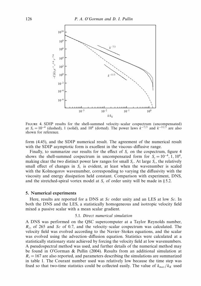
Figure 4. SDIP results for the shell-summed velocity–scalar cospectrum (uncompensated)at Sc = 10−4 (dashed), 1 (solid), and 104 (dotted). The power laws k−7/3 and k−11/3 are alsoshown for reference.

form (4.45), and the SDIP numerical result. The agreement of the numerical resultwith the SDIP asymptotic form is excellent in the viscous–diffusive range.

Finally, to summarize our results for the effect of Sc on the cospectrum, figure 4shows the shell-summed cospectrum in uncompensated form for Sc = 10−4, 1, 104,making clear the two distinct power law ranges for small Sc. At large Sc, the relativelysmall effect of changes in Sc is evident, at least when the wavenumber is scaledwith the Kolmogorov wavenumber, corresponding to varying the diffusivity with theviscosity and energy dissipation held constant. Comparison with experiment, DNS,and the stretched-spiral vortex model at Sc of order unity will be made in § 5.2.

5. Numerical experimentsHere, results are reported for a DNS at Sc order unity and an LES at low Sc. In

both the DNS and the LES, a statistically homogeneous and isotropic velocity fieldmixed a passive scalar with a mean scalar gradient.

5.1. Direct numerical simulation

A DNS was performed on the QSC supercomputer at a Taylor Reynolds number,Rλ, of 265 and Sc of 0.7, and the velocity–scalar cospectrum was calculated. Thevelocity field was evolved according to the Navier–Stokes equations, and the scalarwas evolved using the advection–diffusion equation. Statistics were calculated at astatistically stationary state achieved by forcing the velocity field at low wavenumbers.A pseudospectral method was used, and further details of the numerical method maybe found in O’Gorman & Pullin (2004). Results from an additional simulation atRλ = 167 are also reported, and parameters describing the simulations are summarizedin table 1. The Courant number used was relatively low because the time step wasfixed so that two-time statistics could be collected easily. The value of kmax/kK used


Grid Rλ Tstat/Teddy Sc kmax/kK Rl θ 2/(µlε)2 k0 l C

5123 265 10.5 0.7 1.05 1901 0.45 1.00 0.482563 167 9.3 0.7 1.00 779 0.38 0.99 0.51

Table 1. Simulation parameters for the stationary period of the DNS. Teddy is the eddy turnovertime, Tstat is the time over which the statistics are collected, kmax is the largest dynamicallyimportant wavenumber, Rl is the Reynolds number based on the integral length scale l, theturbulent length scale is lε = u3

rms/ε where urms is the root-mean-square velocity, k0 is thesmallest wavenumber, and C is the Courant number.

10–2 10–1 100

1

2

34(a) (b)

k/kK

10–2 10–1 100

k/kK

E(k

) ε–1

/4 ν

–5/4

(k/

k K)5/

3

Θ(k

) ε3/

4 ν–5

/4 ε

θ–1 (

k/k K

)5/3

0.2

0.4

0.6

0.81.01.21.4

Figure 5. Compensated spectra from the DNS at 5123 (solid line) and 2563 (dashed line):(a) energy spectra, (b) scalar spectra.

is at the low end of the range of commonly used values when passive scalar statisticsare collected at Sc = 0.7.

For both simulations, the shell-summed energy spectra are shown in figure 5(a), andthe shell-summed scalar spectra are shown in figure 5(b). These spectra are shown incompensated form, and are useful as a reference when considering the velocity–scalarcospectrum. A small inertial range and a bump in the dissipation range are apparentfor the energy spectra. The slope of the scalar spectra in the convective range isshallower than k−5/3, although it could be argued that a true inertial–convective rangeis not apparent at these Reynolds numbers.

The shell-summed velocity–scalar cospectra for the two simulations are shown incompensated form in figure 6(a). The cospectral slope is shallower than k−7/3 in theinertial–convective range. Note that the cospectra for the simulations at Rλ of 265 and167 do not exactly coincide for intermediate or large wavenumber, at least with thenormalization used. This is in contrast to the energy and scalar spectra in figures 5(a)and 5(b) which appear to show a universal (Rλ independent) wavenumber range.Mydlarski (2003) also found a dependence on Rλ for the related one-dimensionalheat flux structure function in the inertial–convective range. Further investigation ata range of different Rλ seems warranted.

The one-dimensional cross-spectrum inequality is closely related to the spectralcoherence, see Bendat & Piersol (1986). Similarly, using the the cospectral inequality


10–2 10–1 100 10–2 10–1 100

1

2

3

4(a) (b)–C

(k) µ

–1 ε

1/4 ν

–7/4

(k/

k K)7/

3

k/kKk/kK

H(k

)

10–3

10–2

10–1

100

k–4/3

Figure 6. DNS results at 5123 (solid line) and 2563 (dashed line): (a) compensatedshell-summed velocity–scalar cospectra, (b) shell-summed spectral coherence compared with ak−4/3 power law.

(3.14) as a guide, we can define a shell-summed spectral coherence,

H (k) =3C(k)2

2E(k)Θ(k), (5.1)

so that H (k) � 1. We note that whereas the definition of the one-dimensional spectralcoherence involves the quadrature spectrum, the shell-summed cross-spectrum is realby definition. The magnitude of H (k) is a measure of how correlated the scalar andvelocity Fourier components are at a given wavenumber, and is clearly a measureof the approach to isotropy at small scales. In figure 6(b), we plot H (k) from theDNS, noting that if the Lumley scaling form (1.2) holds, then H (k) will have a k−4/3

wavenumber-dependence in the inertial–convective range. The slope in the inertial–convective range is shallower than k−4/3. The maximum value of H (k) is approximately0.6 and this occurs at the lowest wavenumber. Note that we have omitted the lowestwavenumber for each simulation in figures 5(a), 5(b) and 6(a) for readability.

Unlike for the normalized cospectra in figure 6(a), we do not expect the spectralcoherence functions to coincide at different Rλ. Assume for the moment that thenormalization used in figure 6(a), namely C(k)µ−1ε1/4ν−7/4, gives an approximatelyuniversal form for the cospectrum when plotted against k/kK . We can also use thestandard universal forms for the energy and scalar spectra as these give good collapseof the energy and scalar spectra in figures 5(a) and 5(b). Then the shell-summedspectral coherence should vary in the same way with Rλ as the non-dimensionalnumber ε−1

θ µ2ν, and this can be expected to have a strong Rλ dependence.

5.2. Comparison of DNS results with theory and experiment

We make a comparison of the DNS results for the cospectrum with the SDIPresult of § 4, the stretched-spiral vortex model of O’Gorman & Pullin (2003), andthe experimental result of Mydlarski & Warhaft (1998). We take Sc = 0.7, except inthe case of the stretched-spiral vortex model where Sc is restricted to be unity. Forthis model we also consider only the component of the cospectrum owing to axialmotion in the vortex structures, see O’Gorman & Pullin (2003) for further details.The experimental result was for the one-dimensional cospectrum of the velocity u1


10–2

100

101

10–2

10–3

10–1

10–3 10–1

k3/kK

100

–C1d

(k3)

µ–1

ε1/

4 ν–7

/4 (

k 3/k

K)7/

4

Figure 7. Comparison of one-dimensional velocity–scalar cospectra from the stretched-spiralvortex model (dashed), experimental data from Mydlarski & Warhaft (1998) at Rλ =582 (solid),DNS at Rλ = 265 (dash-dot-dotted), SDIP inertial-convective (dotted), and SDIP (dash-dotted).

and temperature, C1d(k3), at Rλ of 582. Note that in the experiment, the direction ofthe scalar gradient, and hence the scalar flux, was perpendicular to the direction inwhich the cospectrum was measured. The experimental data were rather noisy, andso we have applied a one-third octave smoothing filter. To make the comparison,we convert the SDIP and stretched-spiral vortex model shell-summed cospectra toone-dimensional cospectra using the following formula derived in O’Gorman & Pullin(2003),

C1d(k3) = 34

∫ ∞

k3

k2 + k23

k3C(k) dk. (5.2)

The one-dimensional cospectrum was calculated directly in the DNS.The cospectra are shown in figure 7 in compensated form, where we have also

shown a straight line representing the inertial–convective SDIP result. The DNScospectrum was calculated by time-averaging a sequence of normalized spectra, andso a rough estimate of the error is given by the time variation at a given wavenumber.At k/kk = 0.05 we found that the standard deviation of the compensated cospectrumC1d(k3)µ

−1ε1/4ν−7/4(k3/kK )7/3 was 0.14. It is difficult to estimate the error in theexperimental cospectrum, but we note that the unfiltered compensated cospectrumhad excursions of the order of half a decade in the inertial–convective range.

The shapes of the cospectra are similar in all cases, although the SDIP cospectrumis closer than the other cospectra to a k−7/3 power law in the inertial–convectiverange. The DNS has a similar spectral slope to that of the experimental result whichwas reported as k−2. The SDIP cospectrum seems to be too large in the inertial–convective range, and in this context it is worth noting that the SDIP value for theObukhov–Corrsin differs from experimental values by a factor of about a half. The


discrepancy may be related to the strong assumption used in the SDIP closure ofstatistical independence between the position function and several other variables.

5.3. Large-eddy simulation at low Sc

A large-eddy simulation (LES) was performed to verify the asymptotic results (3.17)and (3.24) for the scalar spectrum and velocity–scalar cospectrum, respectively, at lowSc in the inertial–diffusive range. Our simulation is similar to the LES of Chasnov(1991), where a comparison was made with the asymptotic form (3.17) for the scalarspectrum. Chasnov found excellent agreement in the far inertial–diffusive range, butthe agreement in the near inertial–diffusive range was not as good. As was the casefor Chasnov, we do not need a subgrid model for the scalar because we resolve thediffusive range. Our subgrid model for the velocity is different from that used byChasnov.

A statistically stationary state was reached in the same way as in the DNS by forcingthe velocity at the low wavenumbers, and with a mean scalar gradient acting as thesource for the scalar variance. The resolution used was 643 gridpoints, at an Rλ of1500, and with Sc = 2 × 10−4. Statistics were collected over thirty large-eddy turnovertimes, and time-averaged spectra are reported. The details of the velocity forcing andthe pseudospectral method are the same as in Pullin (2000). We used the stretched-vortex SGS model of Misra & Pullin (1997), with vortex alignment according to thelocally resolved strain rates (model 1a), and a spiral-vortex-type energy spectrum atthe subgrid scales. Evaluation of the second-order velocity structure function was usedto calculate the subgrid energy, see Voelkl, Pullin & Chan (2000) and Pullin (2000)for further details. This LES method has the advantage of dynamically giving a valuefor the Kolmogorov constant. The time-averaged value was K = 1.40 with a standarddeviation of 0.05, which may be compared with the more commonly accepted valueof K = 1.6 (Sreenivasan 1995) We evaluate expressions (3.17) and (3.24) using thevalue for K dynamically calculated by the LES because we need a value of K that isconsistent with the energy spectrum in the LES in order to test the validity of theseasymptotic expressions fairly.

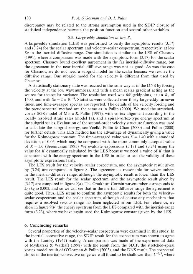
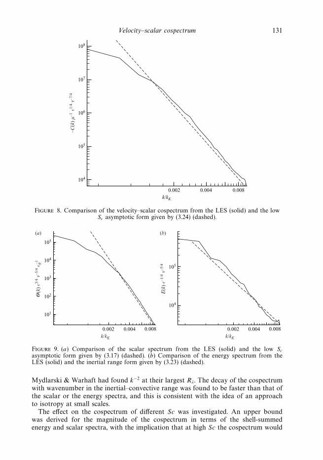
The LES result for the velocity–scalar cospectrum, and the asymptotic result givenby (3.24) are compared in figure 8. The agreement is reasonable for wavenumbersin the inertial–diffusive range, although the asymptotic result is lower than the LESresult. The LES result for the scalar spectrum, and the asymptotic result given by(3.17) are compared in figure 9(a). The Obukhov–Corrsin wavenumber corresponds tokC/kK 0.002, and so we can see that in the inertial–diffusive range the agreement isquite good. Thus, LES seems to confirm the asymptotic results for both the velocity–scalar cospectrum and the scalar spectrum, although of course any mechanism thatrequires a resolved viscous range has been neglected in our LES. For reference, weshow in figure 9(b) the energy spectrum from the LES compared with the inertial-rangeform (3.23), where we have again used the Kolmogorov constant given by the LES.

6. Concluding remarksSeveral properties of the velocity–scalar cospectrum were examined in this study. In

the inertial–convective range, the SDIP result for the cospectrum was shown to agreewith the Lumley (1967) scaling. A comparison was made of the experimental dataof Mydlarski & Warhaft (1998) with the result from the SDIP, the stretched-spiralvortex model result of O’Gorman & Pullin (2003), and the DNS result. The cospectralslopes in the inertial–convective range were all found to be shallower than k−7/3, where


k/kK

0.0040.002 0.008

104

105

106

107

108

–C(k

) µ

–1 ε

1/4 ν

–7/4

Figure 8. Comparison of the velocity–scalar cospectrum from the LES (solid) and the lowSc asymptotic form given by (3.24) (dashed).

101

102

103

104

105

Θ(k

) ε3/

4 ν–5

/4 ε

θ–1

0.0040.002 0.008

E(k

) ε–1

/4 ν

–5/4

104

105

k/kK

0.0040.002 0.008k/kK

(a) (b)

Figure 9. (a) Comparison of the scalar spectrum from the LES (solid) and the low Sc

asymptotic form given by (3.17) (dashed). (b) Comparison of the energy spectrum from theLES (solid) and the inertial range form given by (3.23) (dashed).

Mydlarski & Warhaft had found k−2 at their largest Rλ. The decay of the cospectrumwith wavenumber in the inertial–convective range was found to be faster than that ofthe scalar or the energy spectra, and this is consistent with the idea of an approachto isotropy at small scales.

The effect on the cospectrum of different Sc was investigated. An upper boundwas derived for the magnitude of the cospectrum in terms of the shell-summedenergy and scalar spectra, with the implication that at high Sc the cospectrum would


decay exponentially with wavenumber in the viscous–convective range. This limitsthe possible contribution of sub-Kolmogorov length scales to the mean scalar flux, aresult that may be important in subgrid modelling of the scalar flux. At low Sc, a newasymptotic form was found for the velocity–scalar cospectrum, with a k−11/3 powerlaw wavenumber-dependence in the inertial-diffusive range. The inertial–diffusiveasymptotic forms for the cospectrum and the scalar spectrum were confirmed usingLES, and are in principle subject to experimental verification, perhaps using a liquidmetal. At least in this regime, the forcing of the scalar fluctuation by the meanscalar gradient is important at large wavenumber for both the scalar spectrum andthe velocity–scalar cospectrum. Although the derivation of the SDIP equation forthe cospectrum was complicated, one advantage of the method is that it was thenrelatively inexpensive to investigate a wide range of Sc. Using the SDIP equation,the asymptotic form of the cospectrum in the inertial–diffusive range was confirmedand extended to the viscous–diffusive range. At high Sc, the SDIP result for thecospectrum was indeed found to decay exponentially in the viscous–convective range,as was expected from the cospectrum inequality.

One possibility for future work, suggested by the DNS results described here, is aninvestigation of the Reynolds-number dependence of the cospectrum when plottedusing Kolmogorov scaling. Another possibility for future work is the calculationof the scalar spectrum using the SDIP in the case of a mean scalar gradient. TheSDIP equation for the passive scalar spectrum would then involve the velocity–scalarcospectrum, so that in a sense some of the work has already been done.

P.A.OG. and D.I.P. were supported in part by the National Science Foundationunder Grant CTS-0227881. The DNS was performed on the QSC supercomputer,and was supported by the Academic Strategic Alliances Program of the AcceleratedStrategic Computing Initiative (ASCI/ASAP) under subcontract no. B341492 of DOEcontract W-7405-ENG-48.

Appendix AHere we will show how the Batchelor et al. (1959) result for the scalar spectrum in

the inertial–diffusive range is modified by the presence of a mean scalar gradient. Inthe inertial–diffusive range, we have shown in § 3.3 that an approximate equation forθ(k, t) is given by neglecting the time derivative in (3.19). Multiplying by a similarexpression for θ (−k, t), and taking an ensemble average gives

θ(k, t)θ(−k, t)κ2k4 = µ2u1(k, t)u1(−k, t)

−(

2π

L

)6 ∑p

∑q

pjqiuj (−k − p, t)ui(k − q, t)θ( p, t)θ(q, t)

+ 2µ

(2π

L

)3

Re

(i∑

q

qiui(−k − q, t)θ(q, t)u1(k, t)

). (A 1)

Again using |q| � k, | p| � k, and assuming the statistical independence of modes atwavenumber q or p with modes at k − q, k, or k − p, we find

θ (k, t)θ (−k, t)κ2k4 = µ2u1(k, t)u1(−k, t)

−(

2π

L

)6 ∑p

∑q

pjqiuj (−k − p, t)ui(k − q, t)θ( p, t)θ(q, t).

(A 2)


This may be simplified to

κ2k4Z(k, t, t) = µ2V 11(k, t, t) + V 11(k, t, t)

(2π

L

)3 ∑q

qjqj Z(q, t, t). (A 3)

The sum over q can be related to the scalar dissipation. Taking the limit L → ∞, andperforming a surface integral in wavenumber space leads to

Θ(k) = 23E(k)κ−2k−4

(µ2 +

εθ

2κ

). (A 4)

We are in the inertial range, and so using the appropriate form of the energy spectrum(3.23) gives the result (3.17), which reduces to the Batchelor et al. (1959) result whenthe mean scalar gradient, µ, is set to zero.

Appendix BThis Appendix outlines the derivation of the closed SDIP equations for the velocity–

scalar cospectrum. Further details of the derivation are given in Appendices C, D,and E.† The exact evolution equations for one-and two-point statistics are derivedin Fourier space in §§ B.1 and B.2. The direct-interaction decompositions are made in§ B.3, and the closed equations are derived in § B.4. Finally, the simplification of theequations for the statistically stationary and axisymmetric case is described in § B.5.

B.1. Equations in Fourier space

We begin by writing the governing equations in Fourier space. The incompressibilityof the velocity field implies that kiui(k, t) = 0. The Navier–Stokes equations (4.1)become[

∂

∂t+ νk2

]ui(k, t) = − i

2

(2π

L

)3

P ijm(k)∑

p

∑q

(k+ p+q=0)

uj (− p, t)um(−q, t), (B 1)

where P ijm(k) = kmP ij (k) + kj P im(k), and the incompressible projection operator is

given by P ij (k) = δij − kikj/k2. The scalar advection–diffusion equation (3.18) becomes(3.19) in Fourier space, but here we will use the equivalent symmetric form,[

∂

∂t+ κk2

]θ (k, t) = −µu1(k, t) − ikj

(2π

L

)3 ∑p

∑q

(k+ p+q=0)

uj (− p, t)θ(−q, t). (B 2)

The evolution equation for the Lagrangian position function (4.4) becomes

∂

∂tψ(k, t |k′, t ′) = −ikj

(2π

L

)3 ∑p

∑q

(k+ p+q=0)

uj (− p, t)ψ(−q, t |k′, t ′), (B 3)

with initial condition

ψ(k, t |k′, t ′) =L3

(2π)6δ3

k+k′, (B 4)

† These are available as a supplement to the online version or from the JFM Editorial Office.Cambridge.


where δ3k + k′ = 1 if k = −k′, and δ3

k + k′ = 0 otherwise. The Fourier transforms of theLagrangian velocity and scalar fields evolve according to

∂

∂tvi(t |k, t ′) = − (2π)6

L3ν

∑p

p2ui( p, t)ψ(− p, t |k, t ′)

− i(2π)9

L6

∑p

∑q

∑r

( p+q+r=0)

rirmrn

r2um( p, t)un(q, t)ψ(r, t |k, t ′), (B 5)

and

∂

∂tθ (L)(t |k, t ′) = −µv1(t |k, t ′) − (2π)6

L3κ

∑p

p2θ ( p, t)ψ(− p, t |k, t ′). (B 6)

This may be seen by taking a time derivative of the Fourier space counterparts of(4.6) and (4.7),

vi(t |k, t ′) =(2π)6

L3

∑k′

ui(k′, t)ψ(−k′, t |k, t ′), (B 7)

and

θ (L)(t |k, t ′) =(2π)6

L3

∑k′

θ(k′, t)ψ(−k′, t |k, t ′). (B 8)

The diffusive term in (B 6) is written incorrectly in the paper by Goto & Kida (1999),although this makes no difference after the SDIP approximations are made.

B.2. Two-point statistics

We will need evolution equations for the two-point quantities Wi(k, t, t ′) and Yi(k, t, t ′),defined by (4.12) and (4.13), respectively. For one-time correlations we have[

∂

∂t+ (ν + κ)k2

]Wi(k, t, t) = −µV 1i(k, t, t)

− ikj

(2π

L

)6 ∑p

∑q

(k+ p+q=0)

uj (− p, t)θ(−q, t)ui(−k, t)

+i

2

(2π

L

)6

P ijm(k)∑

p

∑q

(−k+ p+q=0)

uj (− p, t)um(−q, t)θ(k, t),

(B 9)

and Yi(k, t, t) = Wi(−k, t, t). For two-time correlations we have that

∂

∂tWi(k, t, t ′) = −µV 1i(k, t, t ′) − κ

(2π)9

L6

∑p

p2 θ ( p, t)ψ(− p, t |k, t ′)ui(−k, t ′), (B 10)

∂

∂tYi(k, t, t ′) = −i

(2π)12

L9

∑p

∑q

∑r

( p+q+r=0)

rirmrn

r2um( p, t)un(q, t)ψ(r, t |k, t ′)θ (−k, t ′)

− ν(2π)9

L6

∑p

p2ui( p, t)ψ(− p, t |k, t ′)θ (−k, t ′). (B 11)


It will be necessary to make use of linear response functions in the SDIP calculation.The Eulerian and Lagrangian scalar response functions are defined as

G(k, t |k′, t ′) =δθ (k, t)

δθ (k′, t ′), (B 12)

G(L)(t |k, k′, t ′) =δθ (L)(t |k, t ′)

δθ (k′, t ′), (B 13)

with evolution equations[∂

∂t+ κk2

]G(k, t |k′, t ′) = −ikj

(2π

L

)3 ∑p

∑q

(k+ p+q=0)

uj (− p, t)G(−q, t |k′, t ′), (B 14)

∂

∂tG(L)(t |k, k′, t ′) = −κ

(2π)6

L3

∑p

p2G( p, t |k′, t ′)ψ(− p, t |k, t ′), (B 15)

and initial conditions

G(k, t ′|k′, t ′) = G(L)(t ′|k, k′, t ′) =L3

(2π)6δ3

k+k′ . (B 16)

Here δ is a functional derivative, and our notation is consistent so that, forexample, δθ (k, t)/δθ (k′, t ′) is a Fourier transform with respect to x, followed by aFourier transform with respect to x ′ of δθ(x, t)/δθ(x ′, t ′). Similarly, we define Eulerianand Lagrangian velocity response functions as

G(E)ij (k, t |k′, t ′) =

δui(k, t)

δuj (k′, t ′)

, (B 17)

G(L)ij (t |k, k′, t ′) =

δvi(t |k, t ′)

δuj (k′, t ′)

, (B 18)

with initial conditions

G(E)ij (k, t ′|k′, t ′) = G

(L)ij (t ′|k, k′, t ′) =

L3

(2π)6δij δ

3k+k′ . (B 19)

Details of the evolution equations for G(E)ij (k, t |k′, t ′) and G

(L)ij (t |k, k′, t ′) may be found

in KG.We will mostly work with the incompressible projection of G

(L)ij (t |k, k′, t ′), and so

we define

Gij (k, t, t ′) =(2π)6

L3G

(L)im (t |k, −k, t ′)P mj (k). (B 20)

B.3. DIA decompositions

The basis of the SDIP is the decomposition of the field variables into the sum ofnon-direct-interaction (NDI) fields, denoted by the superscript (0), and the deviationfields, denoted with the superscript (1). For example, we decompose the scalar fieldas

θ(k, t) = θ (0)(k, t‖k0, p0, q0) + θ (1)(k, t‖k0, p0, q0), (B 21)

where k0, p0 and q0 are a triad of wavevectors such that k0 + p0 + q0 = 0. The initialconditions for this decomposition are given at time t0 as

θ (0)(k, t0‖k0, p0, q0) = θ (k, t0), θ (1)(k, t0‖k0, p0, q0) = 0. (B 22)


The evolution of θ (0) is governed by[∂

∂t+ κk2

]θ (0)(k, t‖k0, p0, q0) = −ikj

(2π

L

)3 ∑p

∑q

′

(k+ p+q=0)

uj (− p, t)θ (0)(−q, t‖k0, p0, q0)

− µu1(k, t), (B 23)

where∑ ∑ ′

denotes a summation that excludes interactions between the triad k0,p0, and q0. Subtracting (B 23) from (B 2) we find[

∂

∂t+ κk2

]θ (1)(k, t‖k0, p0, q0) = −ikj

(2π

L

)3 ∑p

∑q

′

(k+ p+q=0)

uj (− p, t)θ (1)(−q, t‖k0, p0, q0)

− iδ3k−k0

k0j uj (− p0, t)θ(0)(−q0, t‖k0, p0, q0)

− iδ3k−k0

k0j uj (−q0, t)θ(0)(− p0, t‖k0, p0, q0)

+ iδ3k+k0

k0j uj ( p0, t)θ(0)(q0, t‖k0, p0, q0)

+ iδ3k+k0

k0j uj (q0, t)θ(0)( p0, t‖k0, p0, q0)

+ (k0 → p0 → q0 → k0). (B 24)

Similar decompositions are made for the Eulerian velocity field, u(k, t), the positionfunction, ψ(k, t |k′, t ′), the Eulerian velocity response function G

(E)ij (k, t |k′, t ′), and the

Lagrangian velocity response function G(L)ij (t |k, k′, t ′), see KG. We also decompose

the Eulerian scalar response function, G(k, t |k′, t ′), see Goto & Kida (1999). Thedeviation fields can then be expressed in terms of the NDI fields and the responsefunctions. For example, the scalar deviation field is given by

θ (1)(k, t‖k0, p0, q0) = −ikj

(2π)9

L6

∫ t

t0

dt ′G(0)(k, t | − k, t ′‖k0, p0, q0)

×[δ3

k−k0uj (− p0, t

′)θ (0)(−q0, t′‖k0, p0, q0)

+ δ3k−k0

uj (−q0, t′)θ (0)(− p0, t

′‖k0, p0, q0)

+ δ3k+k0

uj ( p0, t′)θ (0)(q0, t

′‖k0, p0, q0)

+ δ3k+k0

uj (q0, t′)θ (0)( p0, t

′‖k0, p0, q0)

+ (k0 → p0 → q0 → k0)]. (B 25)

B.4. Evolution equations for W (k, t, t), W (k, t, t ′) and X(k, t, t ′)

The main purpose of the SDIP is to express third-order correlations in termsof second-order correlations so that closed evolution equations for second-orderquantities can be derived. There are three main assumptions in the SDIP procedure:(i) The magnitude of the deviation field is smaller than that of the NDI field for times(t−t0) within the correlation time scale of the velocity field. (ii) Any two Fourier modesof the NDI fields without direct interaction are statistically independent of each other.For example, θ (0)(k0, t‖k0, p0, q0), θ (0)( p0, t

′‖k0, p0, q0) and u(0)k (q0, t

′′‖k0, p0, q0) arestatistically independent. (iii) The NDI position function field, ψ (0), is statisticallyindependent of the other Eulerian quantities, such as u

(0)i and θ (0). Additional statistical

assumptions were required in KG involving the position response function, but thisfunction is not used here.


Assumptions (i) and (ii) were tested for a model system in Goto & Kida (1998,2002), but assumption (iii) is difficult to justify. Assumption (iii) will be used severaltimes throughout the derivation to reduce Lagrangian averages, expressed using theposition function, to simpler Eulerian averages. It could be argued that this crudetreatment of the statistics of the position function means that the SDIP is not a trulyLagrangian closure theory. We nonetheless proceed with this assumption as it leadsto a tractable closure.

SDIP approximations to (B 9) and (B 10) are derived in Appendix C using theDIA decompositions and the above three assumptions, and following the methodintroduced by KG and Goto & Kida (1999). The results are[

∂

∂t+ (ν + κ)k2

]Wi(k, t, t) =

(2π

L

)3 ∑p

∑q

(k+ p+q=0)

∫ t

t0

dt ′Li(k, p, q, t, t ′)

− µV 1i(k, t, t), (B 26)

where

Li(k, p, q, t, t ′)

= kj (Qib(−k, t, t ′)Wc(−q, t, t ′)[pcGjb(− p, t, t ′) + pbGjc(− p, t, t ′)]

+ (i ↔ j, k ↔ p)) + kjql exp[−κq2(t − t ′)][Qjl(− p, t, t ′)Xi(−k, t, t ′)

+ Qil(−k, t, t ′)Xj (− p, t, t ′)] + P ijm(k)(Qmc(q, t, t ′)Wb(k, t, t ′)[pcGjb( p, t, t ′)

+ pbGjc( p, t, t ′)] + 12klP ijm(k)exp[−κk2(t − t ′)][Qjl( p, t, t ′)Xm(q, t, t ′)

+ Qml(q, t, t ′)Xj ( p, t, t ′)], (B 27)

and [∂

∂t+ κk2

]Wi(k, t, t ′) = −µV 1i(k, t, t ′). (B 28)

It is easier to work with Xi(k, t, t ′), defined by (4.15), rather than Y i(k, t, t ′), andso the SDIP approximation to the incompressible projection of (B 11) is derived inAppendix D,[

∂

∂t+ νk2

]Xi(k, t, t ′)

= −2

(2π

L

)3 ∑p

∑q

(k+ p+q=0)

P il(k)qlqmqnqj

q2Xn(k, t, t ′)

∫ t

t ′dt ′′Qmj ( p, t, t ′′). (B 29)

Taking the L → ∞ limit, the system of integro-differential equations to be solved canbe summarized as[

∂

∂t+ (ν + κ)k2

]Wi(k, t, t) =

∫d p

∫dqδ3

k+ p+q

∫ t

t0

dt ′Li(k, p, q, t, t ′)

− µV 1i(k, t, t), (B 30)[∂

∂t+ νk2

]Xi(k, t, t ′)

= −2P il(k)

∫d p

∫dqδ3

k+ p+qqlqmqnqj

q2Xn(k, t, t ′)

∫ t

t ′dt ′′Qmj ( p, t, t ′′), (B 31)


together with (B 28) for Wi(k, t, t ′) and the initial condition,

Xi(k, t, t) = Wi(−k, t, t). (B 32)

This is a closed system of equations for Wi(k, t, t ′) and Xi(k, t, t ′) once the velocityfield statistics V ij (k, t, t ′), Qij (k, t, t ′) and Gij (k, t, t ′) are specified.

B.5. Spatial symmetries and stationarity

We now use the spatial symmetries and stationarity of the problem to simplify ourequations. The velocity field is isotropic and stationary, and so we can write (4.16)and

Gij (k, t, t ′) = P ij (k)G†(k, t − t ′). (B 33)

Note that although Gij (k, t, t ′) does not satisfy kiGij (k, t, t ′) = 0 in the general case,

the incompressible property kj Gij (k, t, t ′) = 0 is sufficient to give the form (B 33) in

the isotropic case. Similarly, the condition kj V ij (k, t, t ′) = 0 together with isotropy issufficient to ensure that

V ij (k, t, t ′) = 12P ij (k)V †(k, t − t ′). (B 34)

The definition (4.1.4) of Qij (k, t, t ′) then implies that V †(k, t) = Q†(k, t).We turn now to statistical quantities involving the scalar. It will be convenient to

generalize briefly to the case of an arbitrary mean scalar gradient µi . Axisymmetryand the condition kiWi(k, t, t ′) = 0 imply that,

Wi(k, t, t ′) = f (k, t, t ′, µ, kjµj )

(µi − ki

ksµs

k2

). (B 35)

The scalar, and therefore Wi(k, t, t ′), depend linearly on the mean scalar gradient µi

after initial fluctuations decay, and so we can write Wi(k, t, t ′) = P ij (k)µjW†(k, t − t ′).

In our case, the mean scalar gradient is in the ‘1’ direction and so we find (4.17).Using a similar argument for the form of Xi(k, t, t ′), we find

Xi(k, t, t ′) = P i1(k)µX†(k, t − t ′). (B 36)

Substituting into (B 28) leads to[∂

∂t+ κk2

]W †(k, t) = − 1

2Q†(k, t), (B 37)

and this may be solved to give (4.18).Making a comparison between the evolution equation for Qij (k, t, t ′) in KG, and

the evolution equation (B 29) for Xi(k, t, t ′) here, it is easy to show that X†(k, t) andQ†(k, t) have the same evolution equation. This can be written as[

∂

∂t+ νk2 + η(k, t)

]X†(k, t) = 0, (B 38)

where

η(k, t) =4π

3k5

∫ ∞

0

dpp10/3J(p2/3

) ∫ t

0

dt ′Q†(kp, t ′), (B 39)

and

J (p) =3

32p5

((1 − p3)4

2p3/2log

[1 + p3/2∣∣1 − p3/2

∣∣]

− 1 + p3

3(3p6 − 14p3 + 3)

). (B 40)


Therefore,

X†(k, t) =Q†(k, t)

Q†(k, 0)W †(k, 0), (B 41)

where we have used (B 32). Finally, we substitute the isotropic forms into theintegro-differential equation (B 30) for Wi(k, t, t). The calculation is made easierby recasting (B 30) in the form Lijµj = 0, for a general scalar gradient µj , and thenproceeding by setting Lii = 0. Using (B 41), and the important relation derived inKG, Q†(k, t) = G†(k, t)Q†(k, 0), and after considerable algebra, we find the integralequation (4.19). Note that we have let (t − t0) → ∞, and this is justified by theexponential decay of Q†(k, t) with respect to t . Extensive use has been made ofrelations between geometric factors such as k2σ (k, p, q) = kjkmP jm( p).

REFERENCES

Batchelor, G. K. 1959 Small-scale variation of convected quantities like temperature in turbulentfluid. Part 1. General discussion and the case of small conductivity. J. Fluid Mech. 5, 113–133.

Batchelor, G. K., Howells, I. D. & Townsend, A. A. 1959 Small-scale variation of convectedquantities like temperature in turbulent fluid. Part 2. The case of large conductivity. J. FluidMech. 5, 134–139.

Bendat, J. & Piersol, A. 1986 Random Data – Analysis and Measurement Procedures, 2nd edn.Wiley.

Bos, W. J. T., Touil, H., Shao, L. & Bertoglio, J. P. 2004 On the behaviour of the velocity–scalarcross-correlation spectrum in the inertial range. Phys. Fluids 16, 3818–3823.

Chasnov, J. R. 1991 Simulation of the inertial–conductive subrange. Phys. Fluids A 3, 1164–1168.

Dimotakis, P. E. & Miller, P. L. 1990 Some consequences of the boundedness of scalar fluctuations.Phys. Fluids A 2, 1919–1920.

Galassi, M., Davies, J., Theiler, J., Gough, B., Jungman, G., Booth, M. & Rossi, F. 2001 GNUScientific Library Reference Manual – 2nd. edn. Network Theory.

Gargett, A. E., Merryfield, W. J. & Holloway, G. 2003 Direct numerical simulation of differentialscalar diffusion in three-dimensional stratified turbulence. J. Phys. Oceanogr. 33, 1758–1782.

Gibson, C. H. 1968 Fine structure of scalar fields mixed by turbulence II. Spectral theory. Phys.Fluids 11, 2316–2327.

Goto, S. & Kida, S. 1998 Direct-interaction approximation and Reynolds-number reversedexpansion for a dynamical system. Physica D 117, 191–214.

Goto, S. & Kida, S. 1999 Pasive scalar spectrum in isotropic turbulence: prediction by theLagrangian direct-interaction approximation. Phys. Fluids 11, 1936–1952.

Goto, S. & Kida, S. 2002 Sparseness of nonlinear coupling: importance in sparse direct-interactionperturbation. Nonlinearity 15, 1499–1520.

Gotoh, T. 1989 Passive scalar diffusion in two-dimensional turbulence in the Lagrangian renor-malized approximation. J. Phys. Soc. Japan 58, 2365–2379.

Gotoh, T., Nagaki, J. & Kaneda, Y. 2000 Passive scalar spectrum in the viscous-convective rangein two-dimensional steady turbulence. Phys. Fluids 12, 155–168.

Herr, S., Wang, L. & Collins, L. R. 1996 EDQNM model of a passive scalar with a uniformmean gradient. Phys. Fluids 8, 1588–1608.

Kaneda, Y. 1981 Renormalized expansions in the theory of turbulence with the use of the Lagrangianposition function. J. Fluid Mech. 107, 131–145.

Kaneda, Y. 1986 Inertial range structure of turbulent velocity and scalar fields in a Lagrangianrenormalized approximation. Phys. Fluids 29, 701–708.

Kaneda, Y. & Yoshida, K. 2004 Small-scale anisotropy in stably stratified turbulence. New J. Phys.6, article 34.

Kida, S. & Goto, S. 1997 A Lagrangian direct-interaction approximation for homogeneous isotropicturbulence. J. Fluid Mech. 345, 307–345.

Kraichnan, R. H. 1959 The structure of isotropic turbulence at very high Reynolds number.J. Fluid Mech. 5, 497–543.


Kraichnan, R. H. 1965 Lagrangian-history closure approximation for turbulence. Phys. Fluids 8,575–598.

Leslie, D. 1973 Developments in the Theory of Turbulence. Oxford University Press.

Lumley, J. L. 1967 Similarity and the turbulent energy spectrum. Phys. Fluids 10, 855–858.

Lundgren, T. S. 1982 Strained spiral vortex model for turbulent fine structure. Phys. Fluids 25,2193–2203.

McComb, W. D. 1990 The Physics of Fluid Turbulence. Oxford University Press.

McComb, W. D., Filipiak, M. J. & Shanmugasundaram, V. 1992 Rederivation and furtherassessment of the LET theory of isotropic turbulence, as applied to passive scalar convection.J. Fluid Mech. 245, 279–300.

Miller, P. L. & Dimotakis, P. E. 1996 Measurements of scalar power spectra in high Schmidtnumber turbulent jets. J. Fluid Mech 308, 129–146.

Misra, A. & Pullin, D. I. 1997 A vortex-based subgrid stress model for large-eddy simulation.Phys. Fluids 9, 2443–2454.

Mydlarski, L. 2003 Mixed velocity–passive scalar statistics in high-Reynolds-number turbulence.J. Fluid Mech. 475, 173–203.

Mydlarski, L. & Warhaft, Z. 1998 Passive scalar statistics in high-Peclet-number grid turbulence.J. Fluid Mech. 358, 135–175.

O’Gorman, P. A. & Pullin, D. I. 2003 The velocity–scalar cross spectrum of stretched spiralvortices. Phys. Fluids 15, 280–291.

O’Gorman, P. A. & Pullin, D. I. 2004 On modal time correlations of turbulent velocity and scalarfields. J. Turbulence 5, article 35.

Pullin, D. I. 2000 A vortex-based model for the subgrid flux of a passive scalar. Phys. Fluids 12,2311–2319.

Shraiman, B. L. & Siggia, E. D. 2000 Scalar turbulence. Nature 405, 639–646.

Sreenivasan, K. R. 1995 On the universality of the Kolmogorov constant. Phys. Fluids 7, 2778–2784.

Tennekes, H. & Lumley, J. L. 1974 A First Course in Turbulence. MIT Press.

Voelkl, T., Pullin, D. I. & Chan, D. C. 2000 A physical-space version of the stretched-vortexsubgrid-stress model for large-eddy simulation. Phys. Fluids 12, 1810–1825.

Warhaft, Z. 2000 Passive scalars in turbulent flows. Annu. Rev. Fluid Mech. 32, 203–240.

Yeung, P. K., Xu, S. & Sreenivasan, K. R. 2002 Schmidt number effects on turbulent transportwith uniform mean scalar gradient. Phys. Fluids 14, 4178–4191.

eﬀectofschmidtnumberonthevelocity–scalar ...pog/src/schmidt_number_cospec_2005.pdf · 114 p. a....

Documents