Regression: Predicting and Relating Quantitative

Features

36-402, Advanced Data Analysis

11 January 2011

Reading: Chapter 1 in Faraway, especially up to p. 17.Optional Readings: chapter 1 of Berk; ch. 20 in Adler (through

p. 386).

Contents

1 Statistics, Data Analysis, Regression 1

2 Guessing the Value of a Random Variable 32.1 Estimating the Expected Value . . . . . . . . . . . . . . . . . . . 3

3 The Regression Function 43.1 Some Disclaimers . . . . . . . . . . . . . . . . . . . . . . . . . . . 4

4 Estimating the Regression Function 74.1 The Bias-Variance Tradeoff . . . . . . . . . . . . . . . . . . . . . 84.2 The Bias-Variance Trade-Off in Action . . . . . . . . . . . . . . . 104.3 Ordinary Least Squares Linear Regression as Smoothing . . . . . 10

5 Linear Smoothers 135.1 k-Nearest-Neighbor Regression . . . . . . . . . . . . . . . . . . . 135.2 Kernel Smoothers . . . . . . . . . . . . . . . . . . . . . . . . . . . 15

1 Statistics, Data Analysis, Regression

Statistics is the science which uses mathematics to study and improve ways ofdrawing reliable inferences from incomplete, noisy, corrupt, irreproducible andotherwise imperfect data.

The subject of most sciences is some aspect of the world around us, orwithin us. Psychology studies minds; geology studies the Earth’s compositionand form; economics studies production, distribution and exchange; mycologystudies mushrooms. Statistics does not study the world, but some of the ways

1

we try to understand the world — some of the intellectual tools of the othersciences. Its utility comes indirectly, through helping those other sciences.

This utility is very great, because all the sciences have to deal with imperfectdata. Data may be imperfect because we can only observe and record a smallfraction of what is relevant; or because we can only observe indirect signs ofwhat is truly relevant; or because, no matter how carefully we try, our dataalways contain an element of noise. Over the last two centuries, statistics hascome to model all such imperfections by modeling them as random processes,and probability has become so central to statistics that we introduce randomevents deliberately (as in sample surveys).1

Statistics, then, uses probability to model inference from data. We try tomathematically understand the properties of different procedures for drawinginferences: Under what conditions are they reliable? What sorts of errors dothey make, and how often? What can they tell us when they work? Whatare signs that something has gone wrong? Like some other sciences, such asengineering, medicine and economics, statistics aims not just at understandingbut also at improvement: we want to analyze data better, more reliably, withfewer and smaller errors, under broader conditions, faster, and with less mentaleffort. Sometimes some of these goals conflict — a fast, simple method mightbe very error-prone, or only reliable under a narrow range of circumstances.

One of the things that people most often want to know about the world ishow different variables are related to each other, and one of the central toolsstatistics has for learning about relationships is regression.2 In 36-401, youlearned how to do linear regression, learned about how it could be used in dataanalysis, and learned about its properties. In this class, we will build on thatfoundation, extending beyond simple linear regression in many directions, toanswer many questions about how variables are related to each other.

This is intimately related to prediction. Being able to make predictionsisn’t the only reason we want to understand relations between variables, butprediction tests our knowledge of relations. (If we misunderstand, we might stillbe able to predict, but it’s hard to see how we could understand and not beable to predict.) So before we go beyond linear regression, we will first look atprediction, and how to predict one variable from nothing at all. Then we willlook at predictive relationships between variables, and see how linear regressionis just one member of a big family of smoothing methods, all of which areavailable to us.

1Two excellent, but very different, histories of statistics are Hacking (1990) and Porter(1986).

2The origin of the name is instructive. It comes from 19th century investigations intothe relationship between the attributes of parents and their children. People who are taller(heavier, faster, . . . ) than average tend to have children who are also taller than average, butnot quite as tall. Likewise, the children of unusually short parents also tend to be closer tothe average, and similarly for other traits. This came to be called “regression towards themean”, or even “regression towards mediocrity”, and the word stuck.

2

2 Guessing the Value of a Random Variable

We have a quantitative, numerical variable, which we’ll imaginatively call Y .We’ll suppose that it’s a random variable, and try to predict it by guessing asingle value for it. (Other kinds of predictions are possible — we might guesswhether Y will fall within certain limits, or the probability that it does so, oreven the whole probability distribution of Y . But some lessons we’ll learn herewill apply to these other kinds of predictions as well.) What is the best valueto guess? Or, more formally, what is the optimal point forecast for Y ?

To answer this question, we need to pick a function to be optimized, whichshould measure how good our guesses are — or equivalently how bad they are,how big an error we’re making. A reasonable start point is the mean squarederror:

MSE(a) ≡ E[(Y − a)2

](1)

So we’d like to find the value r where MSE(a) is smallest.

MSE(a) = E[(Y − a)2

](2)

= (E [Y − a])2 + Var [Y − a] (3)

= (E [Y − a])2 + Var [Y ] (4)

= (E [Y ]− a)2 + Var [Y ] (5)dMSEda

= 2 (E [Y ]− a) + 0 (6)

2(E [Y ]− r) = 0 (7)r = E [Y ] (8)

So, if we gauge the quality of our prediction by mean-squared error, the bestprediction to make is the expected value.

2.1 Estimating the Expected Value

Of course, to make the prediction E [Y ] we would have to know the expectedvalue of Y . Typically, we do not. However, if we have sampled values, y1, y2, . . . yn,we can estimate the expectation from the sample mean:

r ≡ 1n

n∑i=1

yi (9)

If the samples are IID, then the law of large numbers tells us that

r → E [Y ] = r (10)

and the central limit theorem tells us something about how fast the convergenceis (namely the squared error will typically be about Var [Y ] /n).

Of course the assumption that the yi come from IID samples is a strongone, but we can assert pretty much the same thing if they’re just uncorrelated

3

with a common expected value. Even if they are correlated, but the correlationsdecay fast enough, all that changes is the rate of convergence. So “sit, wait, andaverage” is a pretty reliable way of estimating the expectation value.

3 The Regression Function

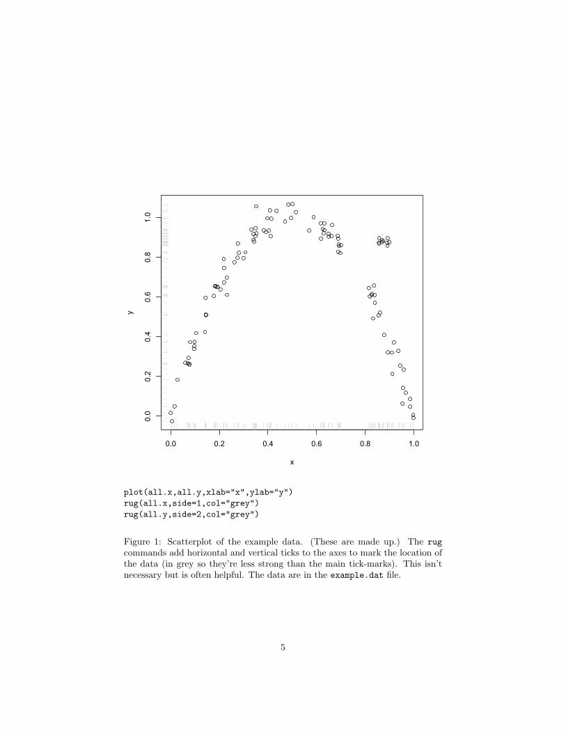
Of course, it’s not very useful to predict just one number for a variable. Typ-ically, we have lots of variables in our data, and we believe they are relatedsomehow. For example, suppose that we have data on two variables, X and Y ,which might look like Figure 1. The feature Y is what we are trying to predict,a.k.a. the dependent variable or output or response, and X is the predic-tor or independent variable or covariate or input. Y might be somethinglike the profitability of a customer and X their credit rating, or, if you wanta less mercenary example, Y could be some measure of improvement in bloodcholesterol and X the dose taken of a drug. Typically we won’t have just oneinput feature X but rather many of them, but that gets harder to draw anddoesn’t change the points of principle.

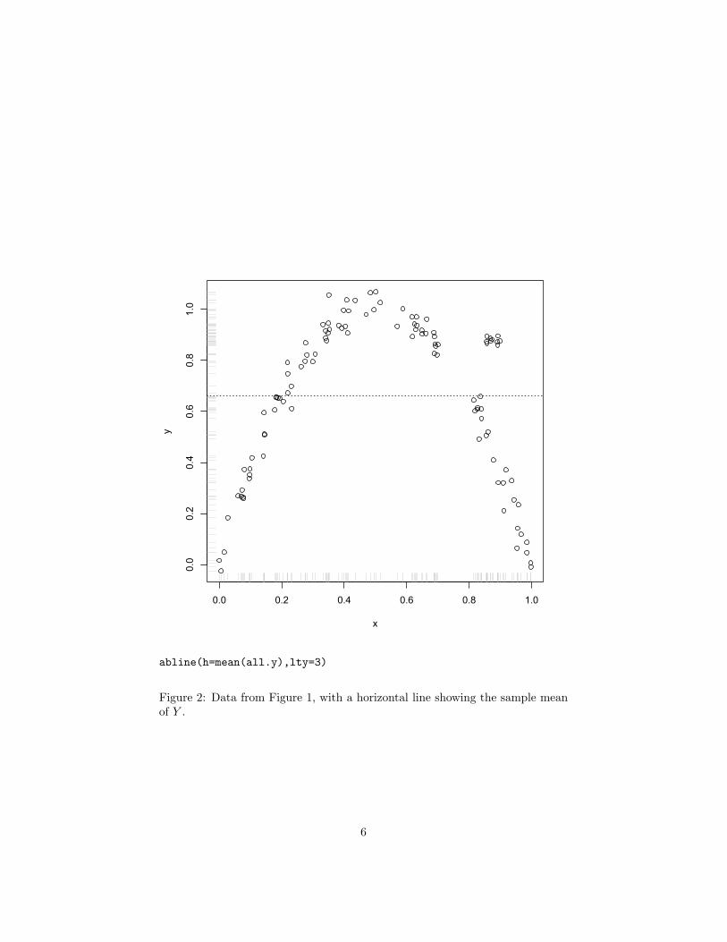
Figure 2 shows the same data as Figure 1, only with the sample mean addedon. This clearly tells us something about the data, but also it seems like weshould be able to do better — to reduce the average error — by using X, ratherthan by ignoring it.

Let’s say that the we want our prediction to be a function of X, namelyf(X). What should that function be, if we still use mean squared error? Wecan work this out by using the law of total expectation, i.e., the fact thatE [U ] = E [E [U |V ]] for any random variables U and V .

MSE(f(X)) = E[(Y − f(X))2

](11)

= E[E[(Y − f(X))2|X

]](12)

= E[Var [Y |X] + (E [Y − f(X)|X])2

](13)

When we want to minimize this, the first term inside the expectation doesn’tdepend on our prediction, and the second term looks just like our previousoptimization only with all expectations conditional on X, so for our optimalfunction r(x) we get

r(x) = E [Y |X = x] (14)

In other words, the (mean-squared) optimal conditional prediction is just theconditional expected value. The function r(x) is called the regression func-tion. This is what we would like to know when we want to predict Y .

3.1 Some Disclaimers

It’s important to be clear on what is and is not being assumed here. Talkingabout X as the “independent variable” and Y as the “dependent” one suggests

4

0.0 0.2 0.4 0.6 0.8 1.0

0.0

0.2

0.4

0.6

0.8

1.0

x

y

plot(all.x,all.y,xlab="x",ylab="y")rug(all.x,side=1,col="grey")rug(all.y,side=2,col="grey")

Figure 1: Scatterplot of the example data. (These are made up.) The rugcommands add horizontal and vertical ticks to the axes to mark the location ofthe data (in grey so they’re less strong than the main tick-marks). This isn’tnecessary but is often helpful. The data are in the example.dat file.

5

0.0 0.2 0.4 0.6 0.8 1.0

0.0

0.2

0.4

0.6

0.8

1.0

x

y

abline(h=mean(all.y),lty=3)

Figure 2: Data from Figure 1, with a horizontal line showing the sample meanof Y .

6

a causal model, which we might write

Y ← r(X) + ε (15)

where the direction of the arrow, ←, indicates the flow from causes to effects,and ε is some noise variable. If the gods of inference are very, very kind, thenε would have a fixed distribution, independent of X, and we could without lossof generality take it to have mean zero. (“Without loss of generality” becauseif it has a non-zero mean, we can incorporate that into r(X) as an additiveconstant.) This is the kind of thing we saw with the factor model. However,no such assumption is required to get Eq. 14. It works when predicting effectsfrom causes, or the other way around when predicting (or “retrodicting”) causesfrom effects, or indeed when there is no causal relationship whatsoever betweenX and Y . It is always true that

Y |X = r(X) + η(X) (16)

where η(X) is a noise variable with mean zero, but as the notation indicatesthe distribution of the noise generally depends on X.

It’s also important to be clear that when we find the regression functionis a constant, r(x) = r0 for all x, that this does not mean that X and Y areindependent. If they are independent, then the regression function is a constant,but turning this around is the logical fallacy of “affirming the consequent”.3

4 Estimating the Regression Function

We want to find the regression function r(x) = E [Y |X = x], and what we’vegot is a big set of training examples, of pairs (x1, y1), (x2, y2), . . . (xn, yn). Howshould we proceed?

If X takes on only a finite set of values, then a simple strategy is to use theconditional sample means:

r(x) =1

# {i : xi = x}∑

i:xi=x

yi (17)

By the same kind of law-of-large-numbers reasoning as before, we can be confi-dent that r(x)→ E [Y |X = x].

Unfortunately, this only works if X has only a finite set of values. If Xis continuous, then in general the probability of our getting a sample at anyparticular value is zero, is the probability of getting multiple samples at exactlythe same value of x. This is a basic issue with estimating any kind of functionfrom data — the function will always be undersampled, and we need to fill

3As in combining the fact that all human beings are featherless bipeds, and the observationthat a cooked turkey is a featherless biped, to conclude that cooked turkeys are human beings.An econometrician stops there; an econometrician who wants to be famous writes a best-sellingbook about how this proves that Thanksgiving is really about cannibalism.

7

in between the values we see. We also need to somehow take into account thefact that each yi is a sample from the conditional distribution of Y |X = xi, andso is not generally equal to E [Y |X = xi]. So any kind of function estimation isgoing to involve interpolation, extrapolation, and smoothing.

Different methods of estimating the regression function — different regres-sion methods, for short — involve different choices about how we interpolate,extrapolate and smooth. This involves our making a choice about how to ap-proximate r(x) by a limited class of functions which we know (or at least hope)we can estimate. There is no guarantee that our choice leads to a good ap-proximation in the case at hand, though it is sometimes possible to say thatthe approximation error will shrink as we get more and more data. This is anextremely important topic and deserves an extended discussion, coming next.

4.1 The Bias-Variance Tradeoff

Suppose that the true regression function is r(x), but we use the function rto make our predictions. Let’s look at the mean squared error at X = x ina slightly different way than before, which will make it clearer what happenswhen we can’t use r to make predictions. We’ll begin by expanding (Y − r(x))2,since the MSE at x is just the expectation of this.

(Y − r(x))2 (18)= (Y − r(x) + r(x)− r(x))2

= (Y − r(x))2 + 2(Y − r(x))(r(x)− r(x)) + (r(x)− r(x))2 (19)

We saw above (Eq. 16) that Y − r(x) = η, a random variable which has ex-pectation zero (and is uncorrelated with x). When we take the expectation ofEq. 19, nothing happens to the last term (since it doesn’t involve any randomquantities); the middle term goes to zero (because E [Y − r(x)] = E [η] = 0),and the first term becomes the variance of η. This depends on x, in general, solet’s call it σ2

x. We have

MSE(r(x)) = σ2x + ((r(x)− r(x))2 (20)

The σ2x term doesn’t depend on our prediction function, just on how hard it is,

intrinsically, to predict Y at X = x. The second term, though, is the extra errorwe get from not knowing r. (Unsurprisingly, ignorance of r cannot improve ourpredictions.) This is our first bias-variance decomposition: the total MSEat x is decomposed into a (squared) bias r(x) − r(x), the amount by whichour predictions are systematically off, and a variance σ2

x, the unpredictable,“statistical” fluctuation around even the best prediction.

All of the above assumes that r is a single fixed function. In practice, ofcourse, r is something we estimate from earlier data. But if those data are ran-dom, the exact regression function we get is random too; let’s call this randomfunction Rn, where the subscript reminds us of the finite amount of data weused to estimate it. What we have analyzed is really MSE(Rn(x)|Rn = r), the

8

mean squared error conditional on a particular estimated regression function.What can we say about the prediction error of the method, averaging over allthe possible training data sets?

MSE(Rn(x)) = E[(Y − Rn(X))2|X = x

](21)

= E[E[(Y − Rn(X))2|X = x, Rn = r

]|X = x

](22)

= E[σ2

x + (r(x)− Rn(x))2|X = x]

(23)

= σ2x + E

[(r(x)− Rn(x))2|X = x

](24)

= σ2x + E

[(r(x)−E

[Rn(x)

]+ E

[Rn(x)

]− Rn(x))2

](25)

= σ2x + (r(x)−E

[Rn(x)

])2 + Var

[Rn(x)

](26)

This is our second bias-variance decomposition — I pulled the same trick asbefore, adding and subtract a mean inside the square. The first term is justthe variance of the process; we’ve seen that before and isn’t, for the moment,of any concern. The second term is the bias in using Rn to estimate r — theapproximation bias or approximation error. The third term, though, is thevariance in our estimate of the regression function. Even if we have an unbiasedmethod (r(x) = E

[Rn(x)

]), if there is a lot of variance in our estimates, we can

expect to make large errors.The approximation bias has to depend on the true regression function. For

example, if E[Rn(x)

]= 42 + 37x, the error of approximation will be zero if

r(x) = 42 + 37x, but it will be larger and x-dependent if r(x) = 0. However,there are flexible methods of estimation which will have small approximationbiases for all r in a broad range of regression functions. The catch is that, atleast past a certain point, decreasing the approximation bias can only comethrough increasing the estimation variance. This is the bias-variance trade-off. However, nothing says that the trade-off has to be one-for-one. Sometimeswe can lower the total error by introducing some bias, since it gets rid of morevariance than it adds approximation error. The next section gives an example.

In general, both the approximation bias and the estimation variance dependon n. A method is consistent4 when both of these go to zero as n→ 0 — thatis, if we recover the true regression function as we get more and more data.5

4To be precise, consistent for r, or consistent for conditional expectations. Moregenerally, an estimator of any property of the data, or of the whole distribution, is consistentif it converges on the truth.

5You might worry about this claim, especially if you’ve taken more probability theory

— aren’t we just saying something about average performance of the R, rather than anyparticular estimated regression function? But notice that if the estimation variance goes to

zero, then by Chebyshev’s inequality each Rn(x) comes arbitrarily close to E

[Rn(x)

]with

arbitrarily high probability. If the approximation bias goes to zero, therefore, the estimatedregression functions converge in probability on the true regression function, not just in mean.

9

Again, consistency depends on how well the method matches the actual data-generating process, not just on the method, and again, there is a bias-variancetrade-off. There can be multiple consistent methods for the same problem, andtheir biases and variances don’t have to go to zero at the same rates.

4.2 The Bias-Variance Trade-Off in Action

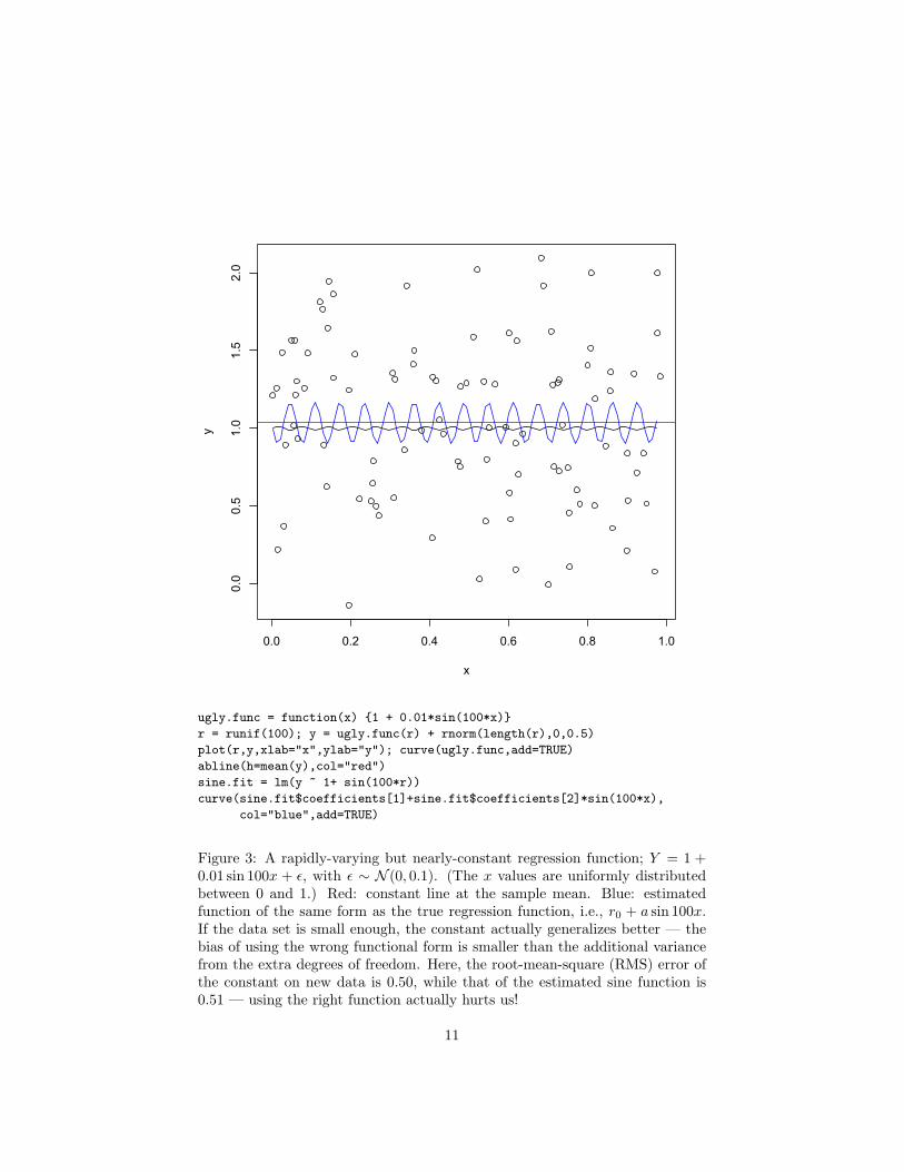
Let’s take an extreme example: we could decide to approximate r(x) by a con-stant r0. The implicit smoothing here is very strong, but sometimes appropri-ate. For instance, it’s appropriate when r(x) really is a constant! Then tryingto estimate any additional structure in the regression function is just so muchwasted effort. Alternately, if r(x) is nearly constant, we may still be better offapproximating it as one. For instance, suppose the true r(x) = r0 + a sin (νx),where a � 1 and ν � 1 (Figure 3 shows an example). With limited data, wecan actually get better predictions by estimating a constant regression functionthan one with the correct functional form.

4.3 Ordinary Least Squares Linear Regression as Smooth-ing

Let’s revisit ordinary least-squares linear regression from this point of view.Let’s assume that the independent variable X is one-dimensional, and that bothX and Y are centered (i.e. have mean zero) — neither of these assumptions isreally necessary, but they reduce the book-keeping.

We choose to approximate r(x) by α + βx, and ask for the best values a, bof those constants. These will be the ones which minimize the mean-squarederror.

MSE(α, β) = E[(Y − α− βX)2

](27)

= E[(Y − α− βX)2|X

](28)

= E[Var [Y |X] + (E [Y − α− βX|X])2

](29)

= E [Var [Y |X]] + E[(E [Y − α− βX|X])2

](30)

The first term doesn’t depend on α or β, so we can drop it for purposes ofoptimization. Taking derivatives, and then brining them inside the expectations,

∂MSE

∂α= E [2(Y − α− βX)(−1)] (31)

E [Y − a− bX] = 0 (32)a = E [Y ]− bE [X] = 0 (33)

using the fact that X and Y are centered; and,

∂MSE

∂β= E [2(Y − α− βX)(−X)] (34)

10

0.0 0.2 0.4 0.6 0.8 1.0

0.0

0.5

1.0

1.5

2.0

x

y

ugly.func = function(x) {1 + 0.01*sin(100*x)}

r = runif(100); y = ugly.func(r) + rnorm(length(r),0,0.5)

plot(r,y,xlab="x",ylab="y"); curve(ugly.func,add=TRUE)

abline(h=mean(y),col="red")

sine.fit = lm(y ~ 1+ sin(100*r))

curve(sine.fit$coefficients[1]+sine.fit$coefficients[2]*sin(100*x),

col="blue",add=TRUE)

Figure 3: A rapidly-varying but nearly-constant regression function; Y = 1 +0.01 sin 100x + ε, with ε ∼ N (0, 0.1). (The x values are uniformly distributedbetween 0 and 1.) Red: constant line at the sample mean. Blue: estimatedfunction of the same form as the true regression function, i.e., r0 + a sin 100x.If the data set is small enough, the constant actually generalizes better — thebias of using the wrong functional form is smaller than the additional variancefrom the extra degrees of freedom. Here, the root-mean-square (RMS) error ofthe constant on new data is 0.50, while that of the estimated sine function is0.51 — using the right function actually hurts us!

11

E [XY ]− bE[X2]

= 0 (35)

b =Cov [X,Y ]

Var [X](36)

again using the centering of X and Y . That is, the mean-squared optimal linearprediction is

r(x) = xCov [X,Y ]

Var [X](37)

Now, if we try to estimate this from data, there are (at least) two approaches.One is to replace the true population values of the covariance and the variancewith their sample values, respectively

1n

∑i

yixi (38)

and1n

∑i

x2i (39)

(again, assuming centering). The other is to minimize the residual sum ofsquares,

RSS(α, β) ≡∑

i

(yi − α− βxi)2 (40)

You may or may not find it surprising that both approaches lead to the sameanswer:

a = 0 (41)

b =∑

i yixi∑i x

2i

(42)

Provided that Var [X] > 0, this will converge with IID samples, so we have aconsistent estimator.6

We are now in a position to see how the least-squares linear regression modelis really a smoothing of the data. Let’s write the estimated regression functionexplicitly in terms of the training data points.

r(x) = bx (43)

= x

∑i yixi∑i x

2i

(44)

=∑

i

yixi∑j x

2j

x (45)

=∑

i

yixi

ns2Xx (46)

6Eq. 41 may look funny, but remember that we’re assuming X and Y have been centered.Centering doesn’t change the slope of the least-squares line but does change the intercept; if

we go back to the un-centered variables the intercept becomes Y − bX, where the bar denotesthe sample mean.

12

where s2X is the sample variance of X. In words, our prediction is a weightedaverage of the observed values yi of the dependent variable, where the weightsare proportional to how far xi is from the center, relative to the variance, andproportional to the magnitude of x. If xi is on the same side of the center asx, it gets a positive weight, and if it’s on the opposite side it gets a negativeweight.

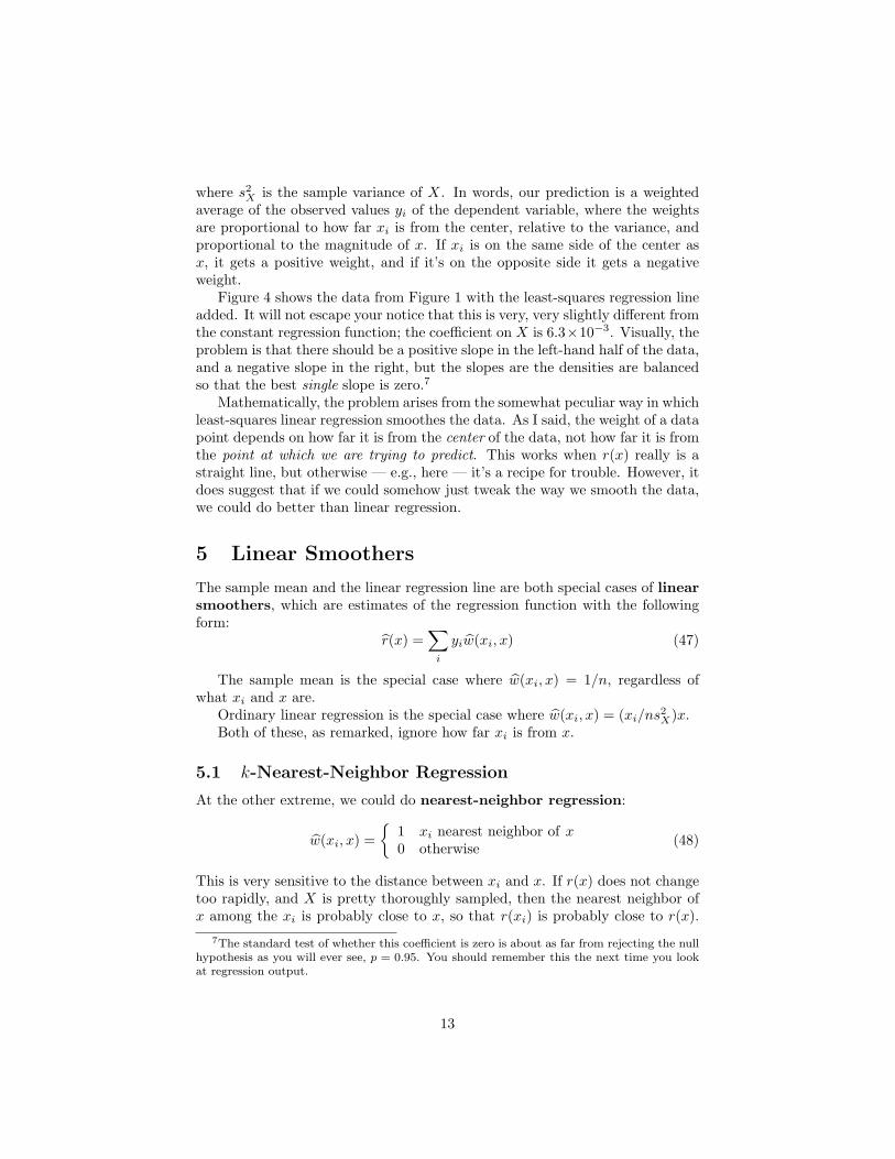
Figure 4 shows the data from Figure 1 with the least-squares regression lineadded. It will not escape your notice that this is very, very slightly different fromthe constant regression function; the coefficient on X is 6.3×10−3. Visually, theproblem is that there should be a positive slope in the left-hand half of the data,and a negative slope in the right, but the slopes are the densities are balancedso that the best single slope is zero.7

Mathematically, the problem arises from the somewhat peculiar way in whichleast-squares linear regression smoothes the data. As I said, the weight of a datapoint depends on how far it is from the center of the data, not how far it is fromthe point at which we are trying to predict. This works when r(x) really is astraight line, but otherwise — e.g., here — it’s a recipe for trouble. However, itdoes suggest that if we could somehow just tweak the way we smooth the data,we could do better than linear regression.

5 Linear Smoothers

The sample mean and the linear regression line are both special cases of linearsmoothers, which are estimates of the regression function with the followingform:

r(x) =∑

i

yiw(xi, x) (47)

The sample mean is the special case where w(xi, x) = 1/n, regardless ofwhat xi and x are.

Ordinary linear regression is the special case where w(xi, x) = (xi/ns2X)x.

Both of these, as remarked, ignore how far xi is from x.

5.1 k-Nearest-Neighbor Regression

At the other extreme, we could do nearest-neighbor regression:

w(xi, x) ={

1 xi nearest neighbor of x0 otherwise (48)

This is very sensitive to the distance between xi and x. If r(x) does not changetoo rapidly, and X is pretty thoroughly sampled, then the nearest neighbor ofx among the xi is probably close to x, so that r(xi) is probably close to r(x).

7The standard test of whether this coefficient is zero is about as far from rejecting the nullhypothesis as you will ever see, p = 0.95. You should remember this the next time you lookat regression output.

13

0.0 0.2 0.4 0.6 0.8 1.0

0.0

0.2

0.4

0.6

0.8

1.0

x

y

fit.all = lm(all.y~all.x)abline(fit.all)

Figure 4: Data from Figure 1, with a horizontal line at the mean (dotted) andthe ordinary least squares regression line (solid). If you zoom in online you willsee that there really are two lines there. (The abline adds a line to the currentplot with intercept a and slope b; it’s set up to take the appropriate coefficientsfrom the output of lm.

14

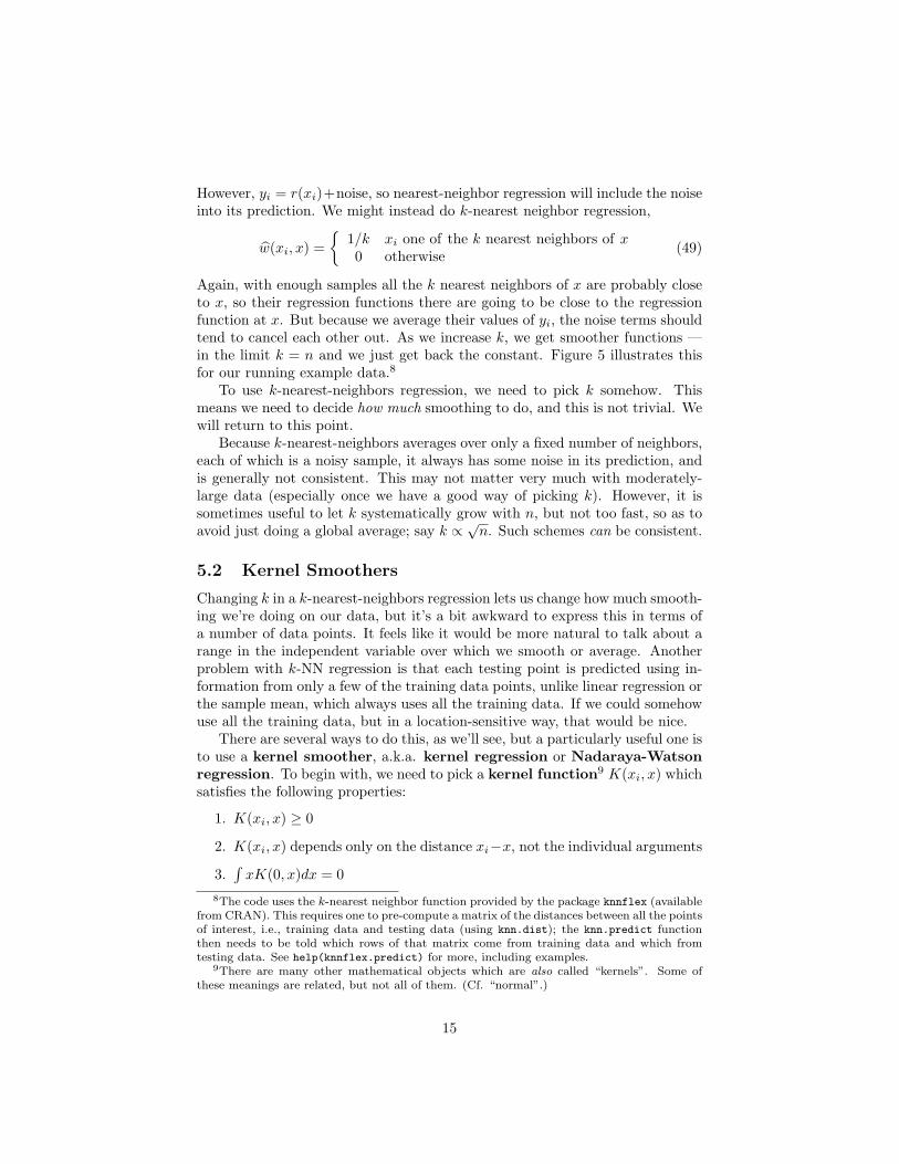
However, yi = r(xi)+noise, so nearest-neighbor regression will include the noiseinto its prediction. We might instead do k-nearest neighbor regression,

w(xi, x) ={

1/k xi one of the k nearest neighbors of x0 otherwise (49)

Again, with enough samples all the k nearest neighbors of x are probably closeto x, so their regression functions there are going to be close to the regressionfunction at x. But because we average their values of yi, the noise terms shouldtend to cancel each other out. As we increase k, we get smoother functions —in the limit k = n and we just get back the constant. Figure 5 illustrates thisfor our running example data.8

To use k-nearest-neighbors regression, we need to pick k somehow. Thismeans we need to decide how much smoothing to do, and this is not trivial. Wewill return to this point.

Because k-nearest-neighbors averages over only a fixed number of neighbors,each of which is a noisy sample, it always has some noise in its prediction, andis generally not consistent. This may not matter very much with moderately-large data (especially once we have a good way of picking k). However, it issometimes useful to let k systematically grow with n, but not too fast, so as toavoid just doing a global average; say k ∝

√n. Such schemes can be consistent.

5.2 Kernel Smoothers

Changing k in a k-nearest-neighbors regression lets us change how much smooth-ing we’re doing on our data, but it’s a bit awkward to express this in terms ofa number of data points. It feels like it would be more natural to talk about arange in the independent variable over which we smooth or average. Anotherproblem with k-NN regression is that each testing point is predicted using in-formation from only a few of the training data points, unlike linear regression orthe sample mean, which always uses all the training data. If we could somehowuse all the training data, but in a location-sensitive way, that would be nice.

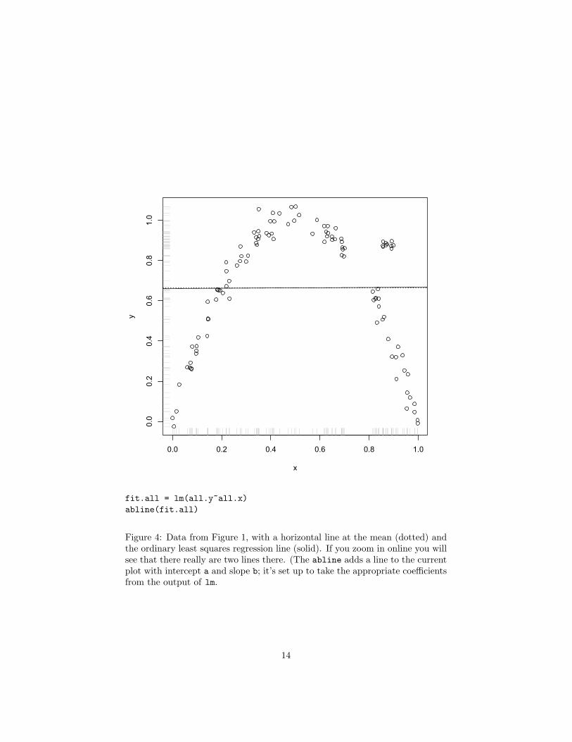
There are several ways to do this, as we’ll see, but a particularly useful one isto use a kernel smoother, a.k.a. kernel regression or Nadaraya-Watsonregression. To begin with, we need to pick a kernel function9 K(xi, x) whichsatisfies the following properties:

1. K(xi, x) ≥ 0

2. K(xi, x) depends only on the distance xi−x, not the individual arguments

3.∫xK(0, x)dx = 0

8The code uses the k-nearest neighbor function provided by the package knnflex (availablefrom CRAN). This requires one to pre-compute a matrix of the distances between all the pointsof interest, i.e., training data and testing data (using knn.dist); the knn.predict functionthen needs to be told which rows of that matrix come from training data and which fromtesting data. See help(knnflex.predict) for more, including examples.

9There are many other mathematical objects which are also called “kernels”. Some ofthese meanings are related, but not all of them. (Cf. “normal”.)

15

0.0 0.2 0.4 0.6 0.8 1.0

0.0

0.2

0.4

0.6

0.8

1.0

x

y

library(knnflex)

all.dist = knn.dist(c(all.x,seq(from=0,to=1,length.out=100)))

all.nn1.predict = knn.predict(1:110,111:210,all.y,all.dist,k=1)

abline(h=mean(all.y),lty=2)

lines(seq(from=0,to=1,length.out=100),all.nn1.predict,col="blue")

all.nn3.predict = knn.predict(1:110,111:210,all.y,all.dist,k=3)

lines(seq(from=0,to=1,length.out=100),all.nn3.predict,col="red")

all.nn5.predict = knn.predict(1:110,111:210,all.y,all.dist,k=5)

lines(seq(from=0,to=1,length.out=100),all.nn5.predict,col="green")

all.nn20.predict = knn.predict(1:110,111:210,all.y,all.dist,k=20)

lines(seq(from=0,to=1,length.out=100),all.nn20.predict,col="purple")

Figure 5: Data points from Figure 1 with horizontal dashed line at the meanand the k-nearest-neighbor regression curves for k = 1 (blue), k = 3 (red),k = 5 (green) and k = 20 (purple). Note how increasing k smoothes out theregression line, and pulls it back towards the mean. (k = 100 would give usback the dashed horizontal line.)

16

4. 0 <∫x2K(0, x)dx <∞

These conditions together (especially the last one) imply that K(xi, x) → 0as |xi − x| → ∞. Two examples of such functions are the density of theUnif(−h/2, h/2) distribution, and the density of the standard GaussianN (0,

√h)

distribution. Here h can be any positive number, and is called the bandwidth.The Nadaraya-Watson estimate of the regression function is

r(x) =∑

i

yiK(xi, x)∑j K(xj , x)

(50)

i.e., in terms of Eq. 47,

w(xi, x) =K(xi, x)∑j K(xj , x)

(51)

(Notice that here, as in k-NN regression, the sum of the weights is always 1.Why?)10

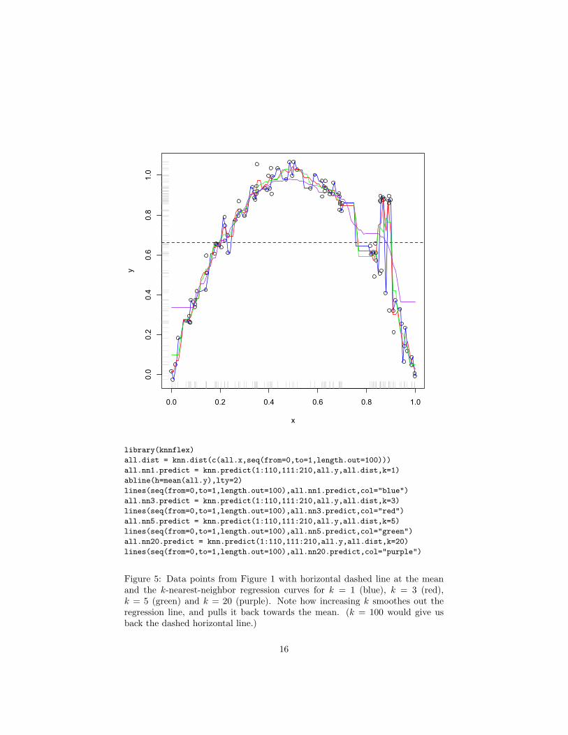
What does this achieve? Well, K(xi, x) is large if xi is close to x, so thiswill place a lot of weight on the training data points close to the point wherewe are trying to predict. More distant training points will have smaller weights,falling off towards zero. If we try to predict at a point x which is very far fromany of the training data points, the value of K(xi, x) will be small for all xi,but it will typically be much, much smaller for all the xi which are not thenearest neighbor of x, so w(xi, x) ≈ 1 for the nearest neighbor and ≈ 0 forall the others.11 That is, far from the training data, our predictions will tendtowards nearest neighbors, rather than going off to ±∞, as linear regression’spredictions do. Whether this is good or bad of course depends on the true r(x)— and how often we have to predict what will happen very far from the trainingdata.

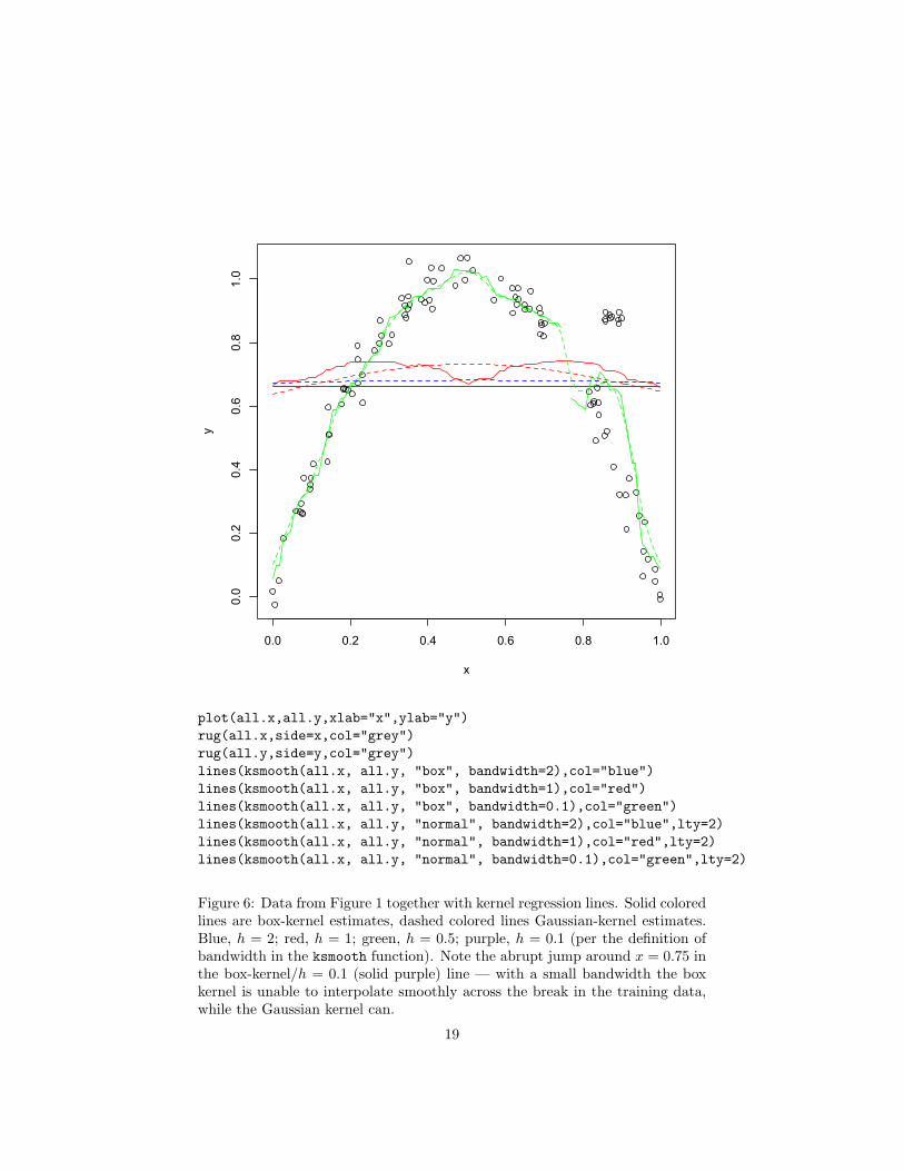
Figure 6 shows our running example data, together with kernel regressionestimates formed by combining the uniform-density, or box, and Gaussian ker-nels with different bandwidths. The box kernel simply takes a region of widthh around the point x and averages the training data points it finds there. TheGaussian kernel gives reasonably large weights to points within h of x, smallerones to points within 2h, tiny ones to points within 3h, and so on, shrinkinglike e−(x−xi)

2/2h. As promised, the bandwidth h controls the degree of smooth-ing. As h → ∞, we revert to taking the global mean. As h → 0, we tend to

10What do we do if K(xi, x) is zero for some xi? Nothing; they just get zero weight inthe average. What do we do if all the K(xi, x) are zero? Different people adopt differentconventions; popular ones are to return the global, unweighted mean of the yi, to do somesort of interpolation from regions where the weights are defined, and to throw up our handsand refuse to make any predictions (computationally, return NA).

11Take a Gaussian kernel in one dimension, for instance, so K(xi, x) ∝ e−(xi−x)2/2h2. Say

xi is the nearest neighbor, and |xi − x| = L, with L � h. So K(xi, x) ∝ e−L2/2h2, a small

number. But now for any other xj , K(xi, x) ∝ e−L2/2h2e−(xj−xi)L/2h2

e−(xj−xi)2/2h2

�e−L2/2h2

. — This assumes that we’re using a kernel like the Gaussian, which never quitegoes to zero, unlike the box kernel.

17

get spikier functions — with the Gaussian kernel at least it tends towards thenearest-neighbor regression.

If we want to use kernel regression, we need to choose both which kernel touse, and the bandwidth to use with it. Experience, like Figure 6, suggests thatthe bandwidth usually matters a lot more than the kernel. This puts us back toroughly where we were with k-NN regression, needing to control the degree ofsmoothing, without knowing how smooth r(x) really is. Similarly again, witha fixed bandwidth h, kernel regression is generally not consistent. However, ifh→ 0 as n→∞, but doesn’t shrink too fast, then we can get consistency.

Next time, we’ll look more at linear regression and some extensions, andthen come back to nearest-neighbor and kernel regression, and say somethingabout how to handle things like the blob of data points around (0.9, 0.9) in thescatter-plot.

References

Hacking, Ian (1990). The Taming of Chance, vol. 17 of Ideas in Context . Cam-bridge, England: Cambridge University Press.

Porter, Theodore M. (1986). The Rise of Statistical Thinking, 1820–1900 .Princeton, New Jersey: Princeton University Press.

18

0.0 0.2 0.4 0.6 0.8 1.0

0.0

0.2

0.4

0.6

0.8

1.0

x

y

plot(all.x,all.y,xlab="x",ylab="y")rug(all.x,side=x,col="grey")rug(all.y,side=y,col="grey")lines(ksmooth(all.x, all.y, "box", bandwidth=2),col="blue")lines(ksmooth(all.x, all.y, "box", bandwidth=1),col="red")lines(ksmooth(all.x, all.y, "box", bandwidth=0.1),col="green")lines(ksmooth(all.x, all.y, "normal", bandwidth=2),col="blue",lty=2)lines(ksmooth(all.x, all.y, "normal", bandwidth=1),col="red",lty=2)lines(ksmooth(all.x, all.y, "normal", bandwidth=0.1),col="green",lty=2)

Figure 6: Data from Figure 1 together with kernel regression lines. Solid coloredlines are box-kernel estimates, dashed colored lines Gaussian-kernel estimates.Blue, h = 2; red, h = 1; green, h = 0.5; purple, h = 0.1 (per the definition ofbandwidth in the ksmooth function). Note the abrupt jump around x = 0.75 inthe box-kernel/h = 0.1 (solid purple) line — with a small bandwidth the boxkernel is unable to interpolate smoothly across the break in the training data,while the Gaussian kernel can.

19

Exercises

These are for you to think through, not to hand in.

1. Suppose we use the mean absolute error instead of the mean squarederror:

MAE(a) = E [|Y − a|] (52)

Is this also minimized by taking a = E [Y ]? If not, what value r minimizesthe MAE? Should we use MSE or MAE to measure error?

2. Derive Eqs. 41 and 42 by minimizing Eq. 40.

3. What does it mean for Gaussian kernel regression to approach nearest-neighbor regression as h → 0? Why does it do so? Is this true for allkinds of kernel regression?

20