using categorical variables in regression analysis€¦ · · 2014-10-30using categorical...
TRANSCRIPT

Using Categorical Variables in
Regression Analysis
Jonas V. Bilenas
Barclays UK&E RBB
PhilaSUG
June 12, 2013
1

Outline
• Quick Review Of Linear Regression Models
• What are Categorical Variables?• Coding up Categorical Variables.• Simple Case Studies:
1. Continuous variable and 2-level categorical variable
2. 2 Continuous variables and a categorical variable with more than 2 levels.
2

Linear Regression Models
3
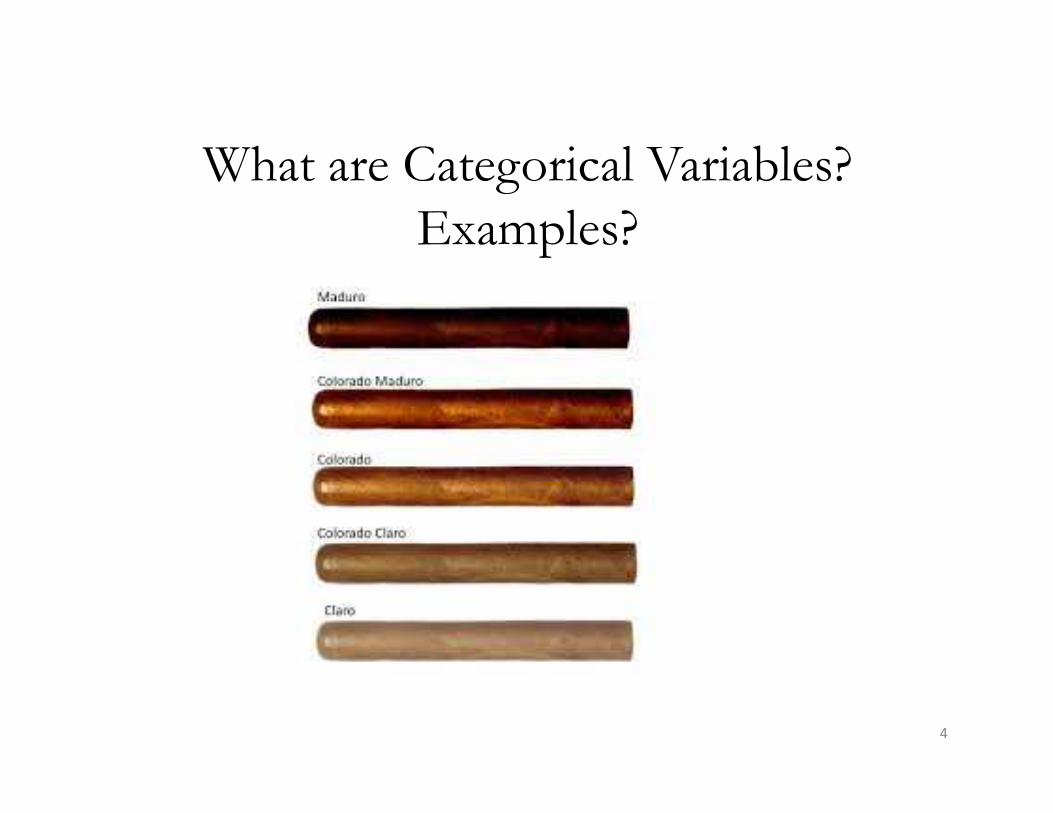
What are Categorical Variables?
Examples?
4
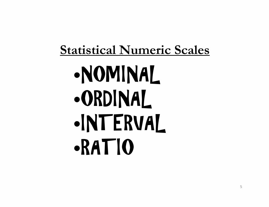
Statistical Numeric Scales
5
•NOMINAL
•ORDINAL•INTERVAL•RATIO

Coding up Categorical Variables?
Most typical coding is called Dummy Coding or Binary Coding. The number of Dummy variables you need is 1 less than the number of levels in the categorical level.
Example: Sex: MALE, FEMALE. You have 2 levels, in the regression model you need 1 dummy variable to code up the categories.
LEVEL SEX
‘MALE’ 1
‘FEMALES’ 0
6

Coding up Categorical Variables? More
than 2 LevelsExample: Sex: MALE, FEMALE, OTHER.
You have 3 levels, in the regression model you need 2 dummy variable to code up the categories.
LEVEL MALE FEMALE
‘MALE’ 1 0
‘FEMALES’ 0 1
OTHER? 0 0
7

CASE STUDY #1:
Predicting Weight of Children as a
function of Height and Sex
8

Regression with continuous and
categorical variables
proc sgplot data=class;REG x=height y=weight/group=sex;xaxis grid;yaxis grid;title Regression Fit of Weight as a Function of Height and Sex;
run;
9
Note: data set CLASS is a modification of SASHELP.CLASS

10

11

Regression with continuous and
categorical variables
proc genmod data=class;class sex;model weight=height | sex
/dist=NOR wald type3 ;run;
12
CLASS: Sets up the coding for you. Be careful that you understand the coding. It may not be DUMMY coding.
TYPE3: Test of the significance of the term after all other terms in the model are added.
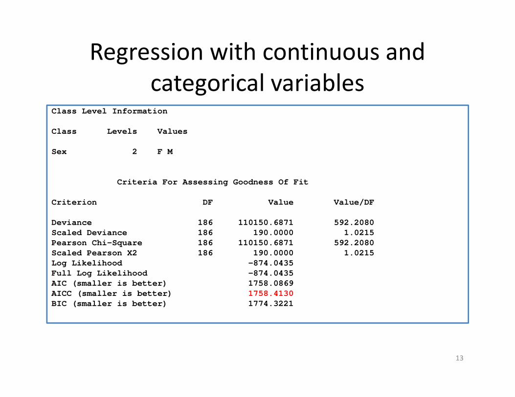
Regression with continuous and
categorical variablesClass Level Information
Class Levels Values
Sex 2 F M
Criteria For Assessing Goodness Of Fit
Criterion DF Value Value/DF
Deviance 186 110150.6871 592.2080Scaled Deviance 186 190.0000 1.0215Pearson Chi-Square 186 110150.6871 592.2080Scaled Pearson X2 186 190.0000 1.0215Log Likelihood -874.0435Full Log Likelihood -874.0435AIC (smaller is better) 1758.0869AICC (smaller is better) 1758.4130BIC (smaller is better) 1774.3221
13

Regression with continuous and
categorical variables
Analysis Of Maximum Likelihood Parameter Estimates
Standard Wald 95% Confidence Wald
Parameter DF Estimate Error Limits Chi-Square Pr > ChiSq
Intercept 1 -215.951 32.9369 -2 80.506 -151.396 42.99 <.0001
Height 1 5.1804 0.5140 4.1730 6.1878 101.58 <.0001
Sex F 1 62.0376 46.3426 -2 8.7923 152.8674 1.79 0.1807
Sex M 0 0.0000 0.0000 0.0000 0.0000 . .
Height*Sex F 1 -1.4834 0.7429 - 2.9395 -0.0273 3.99 0.0459
Height*Sex M 0 0.0000 0.0000 0.0000 0.0000 . .
Scale 1 24.0778 1.2352 2 1.7746 26.6246
2 Regression Equations:
For Males: Weight = -215.951 + 5.1804*Height + e
For Females: Weight = (-215.051+62.0376) +(5.1804 + -1.4834)*Height + e
14

Effect Plots
proc genmod data=class;class sex;model weight = Height | Sex
/ dist=nor link=IDENTITY type3 wald;effectplot fit(x=Height plotby=sex);
run; quit;
15

Regression with continuous and
categorical variables
16

Graphical View
proc sgplot data=class;loess x=height y=weight/group=sex
smooth=0.6;xaxis grid;yaxis grid;title Loess Fit of Weight as a
Function of Height and Sex;run;
Note: data set CLASS is a modification of SASHELP.CLASS
17

Graphical View
18

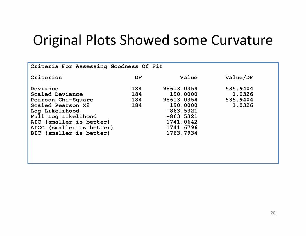
Original Plots Showed some Curvature
proc genmod data=class;
class sex;
model weight = Height | Sex
Height*Height | sex
/ dist=nor link=IDENTITY type3 wald;
effectplot fit(x=Height plotby=sex);
run; quit;
19
Original Plots Showed some Curvature
Criteria For Assessing Goodness Of Fit
Criterion DF Value Value/DF
Deviance 184 98613.0354 535.9404Scaled Deviance 184 190.0000 1.0326Pearson Chi-Square 184 98613.0354 535.9404Scaled Pearson X2 184 190.0000 1.0326Log Likelihood -863.5321Full Log Likelihood -863.5321AIC (smaller is better) 1741.0642AICC (smaller is better) 1741.6796BIC (smaller is better) 1763.7934
20

Original Plots Showed some Curvature
Analysis Of Maximum Likelihood Parameter Estimates
Standard Wald 95% Confidence Wald
Parameter DF Estimate Error Limits Chi-Square Pr > ChiSq
Intercept 1 -1265.20 440.8444 -2129.24 -401.161 8.24 0.0041
Height 1 38.1508 13.8265 11.0514 65.2503 7.61 0.0058
Sex F 1 -523.122 597.3555 -1693.92 647.6737 0.77 0.3812
Sex M 0 0.0000 0.0000 0.0000 0.0000 . .
Height*Sex F 1 21.1722 19.4562 -16.9614 59.3057 1.18 0.2765
Height*Sex M 0 0.0000 0.0000 0.0000 0.0000 . .
Height*Height 1 -0.2576 0.1080 -0.4692 -0.0460 5.69 0.0170
Height*Height*Sex F 1 -0.2124 0.1582 -0.5224 0.0976 1.80 0.1793
Height*Height*Sex M 0 0.0000 0.0000 0.0000 0.0000 . .
Wald Statistics For Type 3 Analysis
Chi-
Source DF Square Pr > ChiS q
Height 1 25.10 <.000 1
Sex 1 0.77 0.381 2
Height*Sex 1 1.18 0.276 5
Height*Height 1 5.69 0.017 0
Height*Height*Sex 1 1.80 0.179 321

Original Plots Showed some Curvature
proc genmod data=class;
class sex;
model weight = Height
Height*Height | sex
/ dist=nor link=IDENTITY type3 wald;
effectplot fit(x=Height plotby=sex);
run; quit;
22
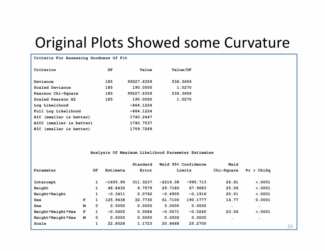
Original Plots Showed some CurvatureCriteria For Assessing Goodness Of Fit
Criterion DF Value Value/DF
Deviance 185 99227.6359 536.3656
Scaled Deviance 185 190.0000 1.0270
Pearson Chi-Square 185 99227.6359 536.3656
Scaled Pearson X2 185 190.0000 1.0270
Log Likelihood -864.1224
Full Log Likelihood -864.1224
AIC (smaller is better) 1740.2447
AICC (smaller is better) 1740.7037
BIC (smaller is better) 1759.7269
Analysis Of Maximum Likelihood Parameter Estimates
Standard Wald 95% Confidence Wald
Parameter DF Estimate Error Limits Chi-Square Pr > ChiSq
Intercept 1 -1605.90 311.3237 -2216.08 -995.713 26.61 <.0001
Height 1 48.8432 9.7579 29.7180 67.9683 25.06 <.0001
Height*Height 1 -0.3411 0.0762 -0.4905 -0.1916 20.01 <.0001
Sex F 1 125.9438 32.7730 61.7100 190.1777 14.77 0.0001
Sex M 0 0.0000 0.0000 0.0000 0.0000 . .
Height*Height*Sex F 1 -0.0405 0.0084 -0.0571 -0.0240 23.04 <.0001
Height*Height*Sex M 0 0.0000 0.0000 0.0000 0.0000 . .
Scale 1 22.8528 1.1723 20.6668 25.270023

Original Plots Showed some Curvature
24

CASE STUDY #2:
Predicting Weight of Children as a
function of Height, Age, and Sex.
Sex at 3 levels
25

Slide 26
What about more than 2 levels. Does it make a difference which level to zero out?
proc genmod data=test2;
class sex;
model weight = height age sex
/ dist=nor link=IDENTITY type3 wald;
run; quit;
The GENMOD Procedure
Model Information
Data Set WORK.TEST2Distribution NormalLink Function IdentityDependent Variable Weight
Number of Observations Read 958Number of Observations Used 958
Class Level Information
Class Levels Values
Sex 3 F M X

Slide 27
Code for PROC GENMOD using GLM coding:
Analysis Of Maximum Likelihood Parameter Estimates
Standard Wald 95% Confidence WaldParameter DF Estimate Error Limits Chi-Square Pr > ChiSq
Intercept 1 -140.323 24.1995 -18 7.754 -92.8933 33.62 <.0001Height 1 2.2739 0.3129 1 .6606 2.8871 52.81 <.0001Age 1 0.8877 1.0815 -1 .2321 3.0074 0.67 0.4118Sex F 1 83.4821 15.9398 52 .2406 114.7236 27.43 <.0001Sex M 1 86.7539 15.2784 56 .8088 116.6990 32.24 <.0001Sex X 0 0.0000 0.0000 0 .0000 0.0000 . . Scale 1 29.7687 0.6801 28 .4651 31.1319
NOTE: The scale parameter was estimated by maximum likelihood.
Wald Statistics For Type 3 Analysis
Chi-Source DF Square Pr > ChiSq
Height 1 52.81 <.0001Age 1 0.67 0.4118Sex 2 41.45 <.0001

Slide 28
• Read documentation for DEFAULT CLASS CODING!
On Tue, 25 Sep 2007 17:01:01 -0700, Richard <[email protected]>
wrote:
>Does anyone know why SAS didn't choose param=ref as the default? It >seems
the obvious choice. >
Maybe because SAS wants you to read the documentation? There is even no
consistency across PROCS. Looking at online documentation for the CLASS
statement, here are the DEFAULT PARAM= codings depending on the PROC:
PROC DEFAULT PARAM
SURVEYLOGISTIC EFFECT
LOGISTIC EFFECT
TPHREG REF
GENMOD GLM
Even if you think you know what you are doing it pays to read the documentation.
Jonas V. Bilenas
http://listserv.uga.edu/cgi-bin/wa?A2=ind0709D&L=sas-l&P=R11996
Slide 29
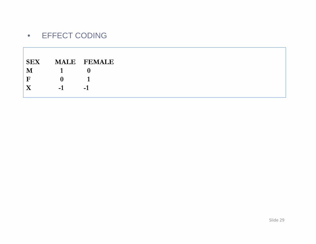
• EFFECT CODING
SEX MALE FEMALE
M 1 0
F 0 1
X -1 -1

Slide 30
Which level of the categorical variable to make the reference?
I like to make it the level with the highest frequency.
The FREQ Procedure
Cumulative CumulativeSex Frequency Percent Frequency Percent--------------------------------------------------------M 500 52.19 500 52.19 F 450 46.97 950 99.16 X 8 0.84 958 100.00
Why? To decrease potential collinearity:

Slide 31
Which level of the categorical variable to make the reference?
To make the highest frequency the reference in GENMOD:
proc genmod data=test2;
class sex/order=freq param=ref ref=first missing;
model weight = height age sex
/ dist=nor link=IDENTITY type3 wald;
run; quit;

Slide 32
Which level of the categorical variable to make the reference in GENMOD?
The GENMOD Procedure
Wald Statistics For Type 3 Analysis
Chi-Source DF Square Pr > ChiSq
Height 1 52.81 <.0001Age 1 0.67 0.4118Sex 2 41.45 <.0001
Analysis Of Maximum Likelihood Parameter Estimates
Standard Wald 95% Confidence WaldParameter DF Estimate Error Limits Chi-Square Pr > ChiSq
Intercept 1 -53.5695 12.3692 -77 .8127 -29.3264 18.76 <.0001Height 1 2.2739 0.3129 1 .6606 2.8871 52.81 <.0001Age 1 0.8877 1.0815 -1 .2321 3.0074 0.67 0.4118Sex F 1 -3.2718 2.1313 -7 .4490 0.9054 2.36 0.1247Sex X 1 -86.7539 15.2784 -11 6.699 -56.8088 32.24 <.0001Scale 1 29.7687 0.6801 28 .4651 31.1319

Slide 33
Additional Reference mentioned during the presentation:
http://www.nesug.org/proceedings/nesug07/sa/sa07.pdf, P.L. Flom, D.L. Cassell, Stopping stepwise: Why stepwise and similar selecti on methods are bad, and what you should use , NESUG 2007.

Slide 34
SAS® is a registered trademark of SAS Institute.
The contents of this paper are the work of the author and do not necessarily represent the
opinions, recommendations, or practices of Barclays or any other company I worked for.
Contact Information:
Email: