logistic regression - · pdf filechapter 11 logistic regression logistic regression analysis...
TRANSCRIPT
Chapter 11
Logistic Regression
Logistic regression analysis is used for predicting the outcome of a categorical
dependent variable based on one or more predictor variables. The probabilities
describing the possible outcomes of a single trial are modeled, as a function of
the explanatory (predictor) variables, using a logistic function. Logistic regres-
sion is frequently used to refer to the problem in which the dependent variable
is binary — that is, the number of available categories is two — and problems
with more than two categories are referred to as multinomial logistic regression
or, if the multiple categories are ordered, as ordered logistic regression.
Logistic regression measures the relationship between a categorical depen-
dent variable and usually (but not necessarily) one or more continuous indepen-
dent variables, by converting the dependent variable to probability scores. As
such it treats the same set of problems as does probit regression using similar
techniques.
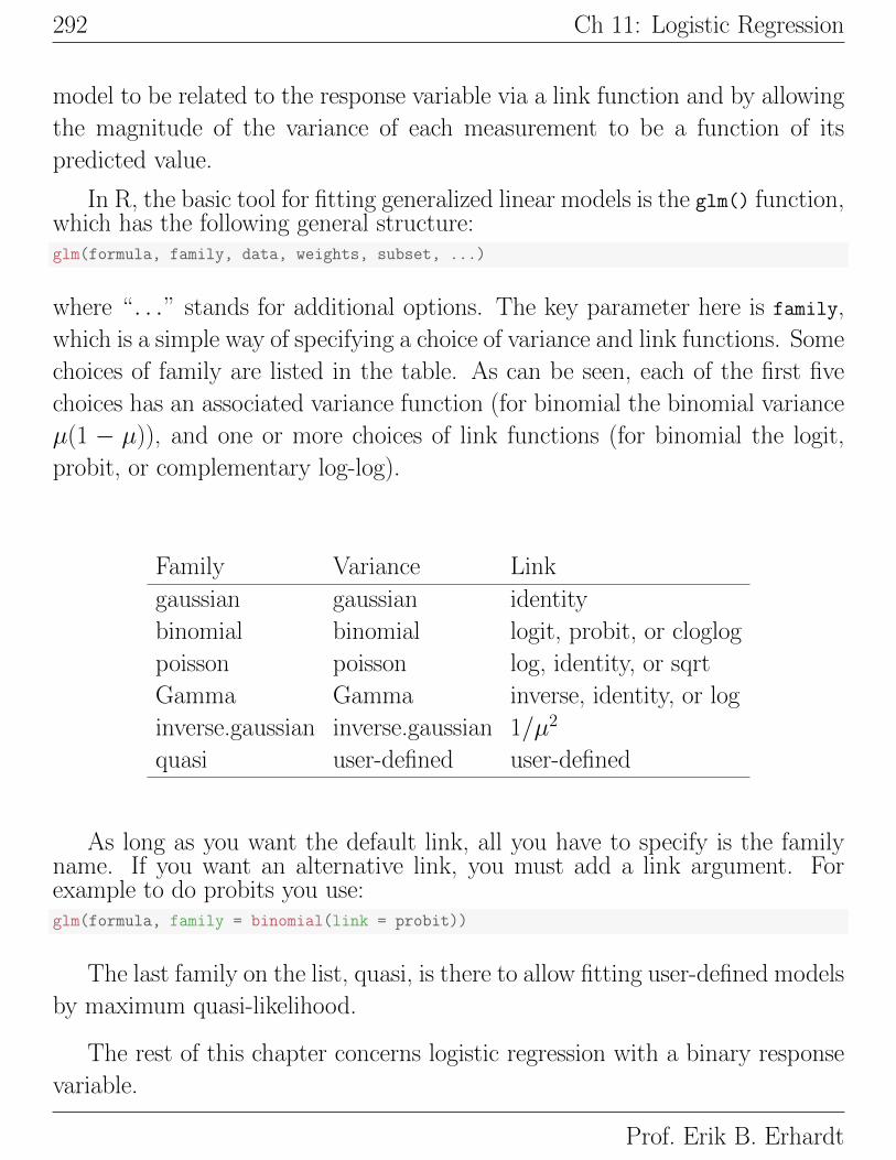
11.1 Generalized linear model variance andlink families
The generalized linear model (GLM) is a flexible generalization of ordinary
linear regression that allows for response variables that have other than a normal
distribution. The GLM generalizes linear regression by allowing the linear
UNM, Stat 428/528 ADA2
292 Ch 11: Logistic Regression
model to be related to the response variable via a link function and by allowing
the magnitude of the variance of each measurement to be a function of its
predicted value.
In R, the basic tool for fitting generalized linear models is the glm() function,which has the following general structure:glm(formula, family, data, weights, subset, ...)
where “...” stands for additional options. The key parameter here is family,
which is a simple way of specifying a choice of variance and link functions. Some
choices of family are listed in the table. As can be seen, each of the first five
choices has an associated variance function (for binomial the binomial variance
µ(1 − µ)), and one or more choices of link functions (for binomial the logit,
probit, or complementary log-log).
Family Variance Link
gaussian gaussian identity
binomial binomial logit, probit, or cloglog
poisson poisson log, identity, or sqrt
Gamma Gamma inverse, identity, or log
inverse.gaussian inverse.gaussian 1/µ2
quasi user-defined user-defined
As long as you want the default link, all you have to specify is the familyname. If you want an alternative link, you must add a link argument. Forexample to do probits you use:glm(formula, family = binomial(link = probit))
The last family on the list, quasi, is there to allow fitting user-defined models
by maximum quasi-likelihood.
The rest of this chapter concerns logistic regression with a binary response
variable.
Prof. Erik B. Erhardt

11.2: Example: Age of Menarche in Warsaw 293
11.2 Example: Age of Menarche in Warsaw
The data1 below are from a study conducted by Milicer and Szczotka on pre-teen
and teenage girls in Warsaw, Poland in 1965. The subjects were classified into
25 age categories. The number of girls in each group (Total) and the number
that reached menarche (Menarche) at the time of the study were recorded. The
age for a group corresponds to the midpoint for the age interval.#### Example: Menarche
# menarche dataset is available in MASS package
# (remove previous instance if it exists, important if rerunning code)
rm(menarche)
library(MASS)
# these frequencies look better in the table as integers
menarche$Total <- as.integer(menarche$Total)
menarche$Menarche <- as.integer(menarche$Menarche)
str(menarche)
## 'data.frame': 25 obs. of 3 variables:
## $ Age : num 9.21 10.21 10.58 10.83 11.08 ...
## $ Total : int 376 200 93 120 90 88 105 111 100 93 ...
## $ Menarche: int 0 0 0 2 2 5 10 17 16 29 ...
# create estimated proportion of girls reaching menarche for each age group
menarche$p.hat <- menarche$Menarche / menarche$Total
1Milicer, H. and Szczotka, F. (1966) Age at Menarche in Warsaw girls in 1965. Human Biology 38,199–203.
UNM, Stat 428/528 ADA2

294 Ch 11: Logistic Regression
Age Total Menarche p.hat1 9.21 376 0 0.002 10.21 200 0 0.003 10.58 93 0 0.004 10.83 120 2 0.025 11.08 90 2 0.026 11.33 88 5 0.067 11.58 105 10 0.108 11.83 111 17 0.159 12.08 100 16 0.16
10 12.33 93 29 0.3111 12.58 100 39 0.3912 12.83 108 51 0.4713 13.08 99 47 0.4714 13.33 106 67 0.6315 13.58 105 81 0.7716 13.83 117 88 0.7517 14.08 98 79 0.8118 14.33 97 90 0.9319 14.58 120 113 0.9420 14.83 102 95 0.9321 15.08 122 117 0.9622 15.33 111 107 0.9623 15.58 94 92 0.9824 15.83 114 112 0.9825 17.58 1049 1049 1.00
The researchers were curious about how the proportion of girls that reached
menarche (p̂ = Menarche/Total) varied with age. One could perform a test
of homogeneity (Multinomial goodness-of-fit test) by arranging the data as a
2-by-25 contingency table with columns indexed by age and two rows: ROW1
= Menarche, and ROW2 = number that have not reached menarche = (Total
− Menarche). A more powerful approach treats these as regression data, using
the proportion of girls reaching menarche as the response and age as a predictor.
A plot of the observed proportion p̂ of girls that have reached menarche
shows that the proportion increases as age increases, but that the relationship
is nonlinear. The observed proportions, which are bounded between zero and
one, have a lazy S-shape (a sigmoidal function) when plotted against age.
The change in the observed proportions for a given change in age is much
smaller when the proportion is near 0 or 1 than when the proportion is near
1/2. This phenomenon is common with regression data where the response is
a proportion.
The trend is nonlinear so linear regression is inappropriate. A sensible al-
ternative might be to transform the response or the predictor to achieve near
linearity. A common transformation of response proportions following a sig-
Prof. Erik B. Erhardt

11.2: Example: Age of Menarche in Warsaw 295
moidal curve is to the logit scale µ̂ = loge{p̂/(1− p̂)}. This transformation
is the basis for the logistic regression model. The natural logarithm (base
e) is traditionally used in logistic regression.
The logit transformation is undefined when p̂ = 0 or p̂ = 1. To overcome this
problem, researchers use the empirical logits, defined by log{(p̂+0.5/n)/(1−p̂+ 0.5/n)}, where n is the sample size or the number of observations on which
p̂ is based.
A plot of the empirical logits against age is roughly linear, which supports
a logistic transformation for the response.library(ggplot2)
p <- ggplot(menarche, aes(x = Age, y = p.hat))
p <- p + geom_point()
p <- p + labs(title = paste("Observed probability of girls reaching menarche,\n","Warsaw, Poland in 1965", sep=""))
print(p)
# emperical logits
menarche$emp.logit <- log(( menarche$p.hat + 0.5/menarche$Total) /
(1 - menarche$p.hat + 0.5/menarche$Total))
library(ggplot2)
p <- ggplot(menarche, aes(x = Age, y = emp.logit))
p <- p + geom_point()
p <- p + labs(title = "Empirical logits")
print(p)
● ● ●● ●
●
●
● ●
●
●
● ●
●
●●
●
●●
●
● ●● ●
●
0.00
0.25
0.50
0.75
1.00
10 12 14 16Age
p.ha
t
Observed probability of girls reaching menarche,Warsaw, Poland in 1965
●
●
●
●●
●
●
● ●
●
●● ●
●
● ●●
●●
●
● ●
●●
●
−4
0
4
8
10 12 14 16Age
emp.
logi
t
Empirical logits
UNM, Stat 428/528 ADA2

296 Ch 11: Logistic Regression
11.3 Simple logistic regression model
The simple logistic regression model expresses the population proportion p of
individuals with a given attribute (called the probability of success) as a function
of a single predictor variable X . The model assumes that p is related to X
through
log
(p
1− p
)= β0 + β1X
or, equivalently, as
p =exp(β0 + β1X)
1 + exp(β0 + β1X).
The logistic regression model is a binary response model, where the re-
sponse for each case falls into one of two exclusive and exhaustive categories,
success (cases with the attribute of interest) and failure (cases without the
attribute of interest).
The odds of success are p/(1 − p). For example, when p = 1/2 the odds
of success are 1 (or 1 to 1). When p = 0.9 the odds of success are 9 (or 9 to
1). The logistic model assumes that the log-odds of success is linearly related
to X . Graphs of the logistic model relating p to X are given below. The sign
of the slope refers to the sign of β1.
I should write p = p(X) to emphasize that p is the proportion of all indi-
viduals with score X that have the attribute of interest. In the menarche data,
p = p(X) is the population proportion of girls at age X that have reached
menarche.
Prof. Erik B. Erhardt

11.3: Simple logistic regression model 297
X
Log-
Odd
s
-5 0 5
-50
5
- slope
+ slope
0 slope
Logit Scale
XP
roba
bilit
y
-5 0 5
0.0
0.2
0.4
0.6
0.8
1.0
0 slope
+ slope - slope
Probability Scale
The data in a logistic regression problem are often given in summarized or
aggregate form:
X n y
X1 n1 y1
X2 n2 y2... ... ...
Xm nm ymwhere yi is the number of individuals with the attribute of interest among nirandomly selected or representative individuals with predictor variable value
Xi. For raw data on individual cases, yi = 1 or 0, depending on whether the
case at Xi is a success or failure, and the sample size column n is omitted with
raw data.
For logistic regression, a plot of the sample proportions p̂i = yi/ni against
Xi should be roughly sigmoidal, and a plot of the empirical logits against Xi
should be roughly linear. If not, then some other model is probably appropriate.
I find the second plot easier to calibrate, but neither plot is very informative
when the sample sizes are small, say 1 or 2. (Why?).
There are a variety of other binary response models that are used in practice.
The probit regression model or the complementary log-log regression
UNM, Stat 428/528 ADA2

298 Ch 11: Logistic Regression
model might be appropriate when the logistic model does fit the data.
The following section describes the standard MLE strategy for estimating
the logistic regression parameters.
11.3.1 Estimating Regression Parameters via LS ofempirical logits
(This is a naive method; we will discuss a better way in the next section.)
There are two unknown population parameters in the logistic regression
model
log
(p
1− p
)= β0 + β1X.
A simple way to estimate β0 and β1 is by least squares (LS), using the empirical
logits as responses and the Xis as the predictor values.Below we use standard regression to calculate the LS fit between the empir-
ical logits and age.lm.menarche.e.a <- lm(emp.logit ~ Age, data = menarche)
# LS coefficients
coef(lm.menarche.e.a)
## (Intercept) Age
## -22.027933 1.676395
The LS estimates for the menarche data are b0 = −22.03 and b1 = 1.68,
which gives the fitted relationship
log
(p̃
1− p̃
)= −22.03 + 1.68 Age
or
p̃ =exp(−22.03 + 1.68 Age)
1 + exp(−22.03 + 1.68 Age),
where p̃ is the predicted proportion (under the model) of girls having reached
menarche at the given age. I used p̃ to identify a predicted probability, in
contrast to p̂ which is the observed proportion at a given age.
The power of the logistic model versus the contingency table analysis dis-
cussed earlier is that the model gives estimates for the population proportion
Prof. Erik B. Erhardt

11.3: Simple logistic regression model 299
reaching menarche at all ages within the observed age range. The observed pro-
portions allow you to estimate only the population proportions at the observed
ages.
11.3.2 Maximum Likelihood Estimation for LogisticRegression Model
There are better ways to the fit the logistic regression model than LS which
assumes that the responses are normally distributed with constant variance.
A deficiency of the LS fit to the logistic model is that the observed counts
yi have a Binomial distribution under random sampling. The Binomial
distribution is a discrete probability model associated with counting the number
of successes in a fixed size sample, and other equivalent experiments such as
counting the number of heads in repeated flips of a coin. The distribution of the
empirical logits depend on the yis so they are not normal (but are approximately
normal in large samples), and are extremely skewed when the sample sizes niare small. The response variability depends on the population proportions, and
is not roughly constant when the observed proportions or the sample sizes vary
appreciably across groups.
The differences in variability among the empirical logits can be accounted
for using weighted least squares (WLS) when the sample sizes are large.
An alternative approach called maximum likelihood uses the exact Binomial
distribution of the responses yi to generate optimal estimates of the regression
coefficients. Software for maximum likelihood estimation is widely available, so
LS and WLS methods are not really needed.
In maximum likelihood estimation (MLE), the regression coefficients
are estimated iteratively by minimizing the deviance function (also called the
likelihood ratio chi-squared statistic)
D = 2
m∑i=1
{yi log
(yinipi
)+ (ni − yi) log
(ni − yini − nipi
)}UNM, Stat 428/528 ADA2

300 Ch 11: Logistic Regression
over all possible values of β0 and β1, where the pis satisfy the logistic model
log
(pi
1− pi
)= β0 + β1Xi.
The ML method also gives standard errors and significance tests for the regres-
sion estimates.
The deviance is an analog of the residual sums of squares in linear regression.
The choices for β0 and β1 that minimize the deviance are the parameter values
that make the observed and fitted proportions as close together as possible in
a “likelihood sense”.
Suppose that b0 and b1 are the MLEs of β0 and β1. The deviance evaluated
at the MLEs,
D = 2
m∑i=1
{yi log
(yinip̃i
)+ (ni − yi) log
(ni − yini − nip̃i
)},
where the fitted probabilities p̃i satisfy
log
(p̃i
1− p̃i
)= b0 + b1Xi,
is used to test the adequacy of the model. The deviance is small when the
data fits the model, that is, when the observed and fitted proportions are close
together. Large values of D occur when one or more of the observed and fitted
proportions are far apart, which suggests that the model is inappropriate.
If the logistic model holds, then D has a chi-squared distribution
with m− r degrees of freedom, where m is the the number of groups and
r (here 2) is the number of estimated regression parameters. A p-value for the
deviance is given by the area under the chi-squared curve to the right of D. A
small p-value indicates that the data does not fit the model.
Alternatively, the fit of the model can be evaluated using the chi-squared
approximation to the Pearson X2 statistic:
X2 =
m∑i=1
{(yi − nip̃i)2
nip̃i+
((ni − yi)− ni(1− p̃i))2
ni(1− p̃i)
}=
m∑i=1
(yi − nip̃i)2
nip̃i(1− p̃i).
Prof. Erik B. Erhardt

11.3: Simple logistic regression model 301
11.3.3 Fitting the Logistic Model by Maximum Like-lihood, Menarche
# For our summarized data (with frequencies and totals for each age)
# The left-hand side of our formula binds two columns together with cbind():
# the columns are the number of "successes" and "failures".
# For logistic regression with logit link we specify family = binomial,
# where logit is the default link function for the binomial family.
glm.m.a <- glm(cbind(Menarche, Total - Menarche) ~ Age, family = binomial, menarche)
The glm() statement creates an object which we can use to create the fit-
ted probabilities and 95% CIs for the population proportions at the ages in
menarche. The fitted probabilities and the limits are stored in columns la-
beled fitted.values, fit.lower, and fit.upper, respectively.# put the fitted values in the data.frame
menarche$fitted.values <- glm.m.a$fitted.values
pred <- predict(glm.m.a, data.frame(Age = menarche$Age), type = "link", se.fit = TRUE)
menarche$fit <- pred$fit
menarche$se.fit <- pred$se.fit
# CI for fitted values
menarche <- within(menarche, {fit.lower = exp(fit - 1.96 * se.fit) / (1 + exp(fit - 1.96 * se.fit))
fit.upper = exp(fit + 1.96 * se.fit) / (1 + exp(fit + 1.96 * se.fit))
})#round(menarche, 3)
This printed summary information is easily interpreted. For example, the
estimated population proportion of girls aged 15.08 (more precisely, among girls
in the age interval with midpoint 15.08) that have reached menarche is 0.967.
You are 95% confident that the population proportion is between 0.958 and
0.975. A variety of other summaries and diagnostics can be produced.
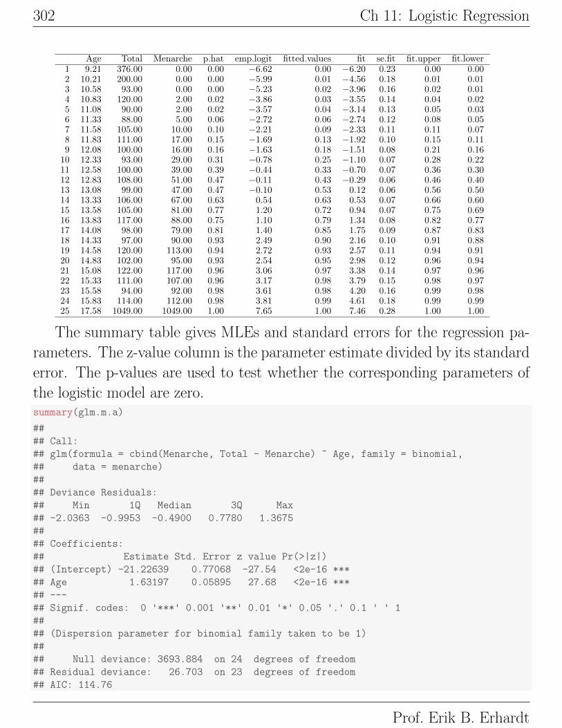
Age Total Menarche p.hat emp.logit fitted.values fit se.fit fit.upper fit.lower21 15.08 122.00 117.00 0.96 3.06 0.97 3.38 0.14 0.97 0.96
UNM, Stat 428/528 ADA2
302 Ch 11: Logistic Regression
Age Total Menarche p.hat emp.logit fitted.values fit se.fit fit.upper fit.lower1 9.21 376.00 0.00 0.00 −6.62 0.00 −6.20 0.23 0.00 0.002 10.21 200.00 0.00 0.00 −5.99 0.01 −4.56 0.18 0.01 0.013 10.58 93.00 0.00 0.00 −5.23 0.02 −3.96 0.16 0.02 0.014 10.83 120.00 2.00 0.02 −3.86 0.03 −3.55 0.14 0.04 0.025 11.08 90.00 2.00 0.02 −3.57 0.04 −3.14 0.13 0.05 0.036 11.33 88.00 5.00 0.06 −2.72 0.06 −2.74 0.12 0.08 0.057 11.58 105.00 10.00 0.10 −2.21 0.09 −2.33 0.11 0.11 0.078 11.83 111.00 17.00 0.15 −1.69 0.13 −1.92 0.10 0.15 0.119 12.08 100.00 16.00 0.16 −1.63 0.18 −1.51 0.08 0.21 0.16
10 12.33 93.00 29.00 0.31 −0.78 0.25 −1.10 0.07 0.28 0.2211 12.58 100.00 39.00 0.39 −0.44 0.33 −0.70 0.07 0.36 0.3012 12.83 108.00 51.00 0.47 −0.11 0.43 −0.29 0.06 0.46 0.4013 13.08 99.00 47.00 0.47 −0.10 0.53 0.12 0.06 0.56 0.5014 13.33 106.00 67.00 0.63 0.54 0.63 0.53 0.07 0.66 0.6015 13.58 105.00 81.00 0.77 1.20 0.72 0.94 0.07 0.75 0.6916 13.83 117.00 88.00 0.75 1.10 0.79 1.34 0.08 0.82 0.7717 14.08 98.00 79.00 0.81 1.40 0.85 1.75 0.09 0.87 0.8318 14.33 97.00 90.00 0.93 2.49 0.90 2.16 0.10 0.91 0.8819 14.58 120.00 113.00 0.94 2.72 0.93 2.57 0.11 0.94 0.9120 14.83 102.00 95.00 0.93 2.54 0.95 2.98 0.12 0.96 0.9421 15.08 122.00 117.00 0.96 3.06 0.97 3.38 0.14 0.97 0.9622 15.33 111.00 107.00 0.96 3.17 0.98 3.79 0.15 0.98 0.9723 15.58 94.00 92.00 0.98 3.61 0.98 4.20 0.16 0.99 0.9824 15.83 114.00 112.00 0.98 3.81 0.99 4.61 0.18 0.99 0.9925 17.58 1049.00 1049.00 1.00 7.65 1.00 7.46 0.28 1.00 1.00
The summary table gives MLEs and standard errors for the regression pa-
rameters. The z-value column is the parameter estimate divided by its standard
error. The p-values are used to test whether the corresponding parameters of
the logistic model are zero.summary(glm.m.a)
##
## Call:
## glm(formula = cbind(Menarche, Total - Menarche) ~ Age, family = binomial,
## data = menarche)
##
## Deviance Residuals:
## Min 1Q Median 3Q Max
## -2.0363 -0.9953 -0.4900 0.7780 1.3675
##
## Coefficients:
## Estimate Std. Error z value Pr(>|z|)
## (Intercept) -21.22639 0.77068 -27.54 <2e-16 ***
## Age 1.63197 0.05895 27.68 <2e-16 ***
## ---
## Signif. codes: 0 '***' 0.001 '**' 0.01 '*' 0.05 '.' 0.1 ' ' 1
##
## (Dispersion parameter for binomial family taken to be 1)
##
## Null deviance: 3693.884 on 24 degrees of freedom
## Residual deviance: 26.703 on 23 degrees of freedom
## AIC: 114.76
Prof. Erik B. Erhardt
11.3: Simple logistic regression model 303
##
## Number of Fisher Scoring iterations: 4
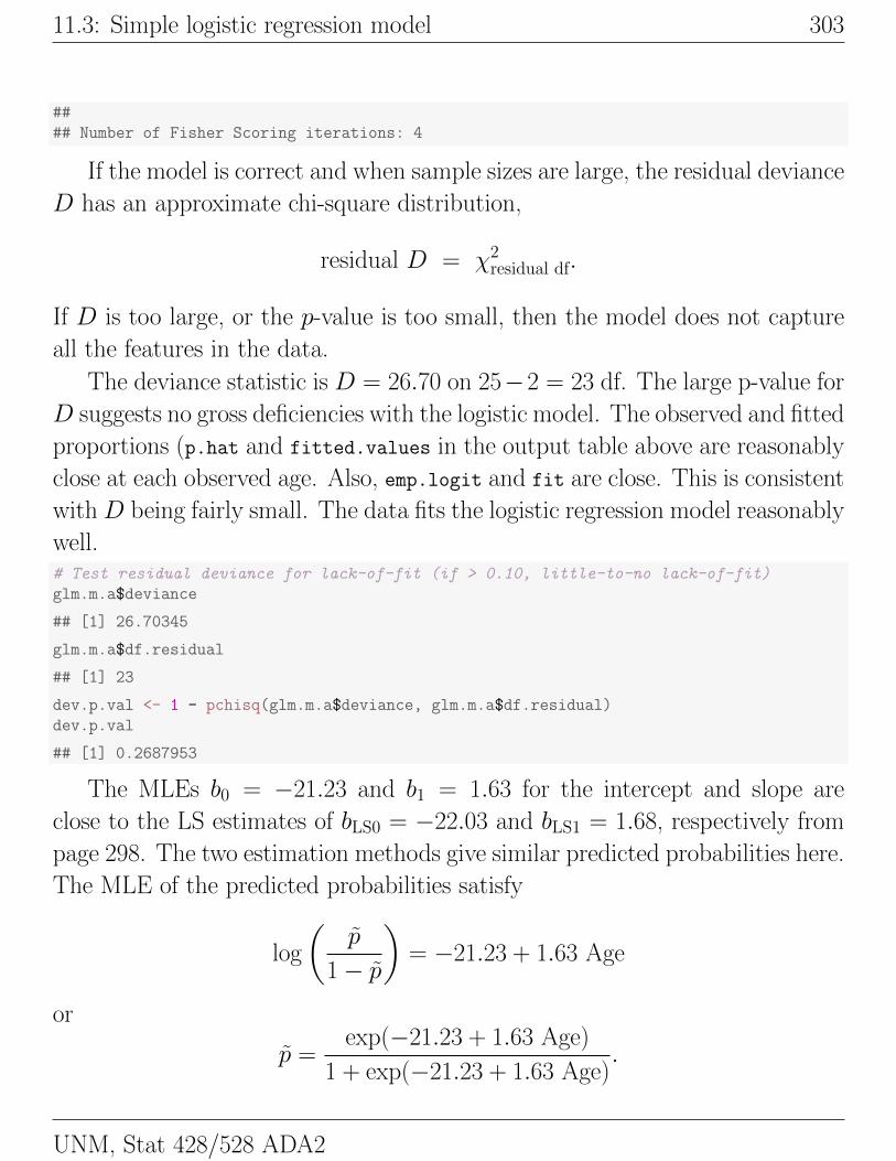
If the model is correct and when sample sizes are large, the residual deviance
D has an approximate chi-square distribution,
residual D = χ2residual df.
If D is too large, or the p-value is too small, then the model does not capture
all the features in the data.
The deviance statistic is D = 26.70 on 25−2 = 23 df. The large p-value for
D suggests no gross deficiencies with the logistic model. The observed and fitted
proportions (p.hat and fitted.values in the output table above are reasonably
close at each observed age. Also, emp.logit and fit are close. This is consistent
with D being fairly small. The data fits the logistic regression model reasonably
well.# Test residual deviance for lack-of-fit (if > 0.10, little-to-no lack-of-fit)
glm.m.a$deviance
## [1] 26.70345
glm.m.a$df.residual
## [1] 23
dev.p.val <- 1 - pchisq(glm.m.a$deviance, glm.m.a$df.residual)
dev.p.val
## [1] 0.2687953
The MLEs b0 = −21.23 and b1 = 1.63 for the intercept and slope are
close to the LS estimates of bLS0 = −22.03 and bLS1 = 1.68, respectively from
page 298. The two estimation methods give similar predicted probabilities here.
The MLE of the predicted probabilities satisfy
log
(p̃
1− p̃
)= −21.23 + 1.63 Age
or
p̃ =exp(−21.23 + 1.63 Age)
1 + exp(−21.23 + 1.63 Age).
UNM, Stat 428/528 ADA2
304 Ch 11: Logistic Regression
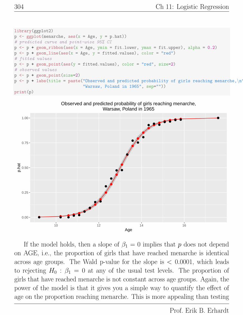
library(ggplot2)
p <- ggplot(menarche, aes(x = Age, y = p.hat))
# predicted curve and point-wise 95% CI
p <- p + geom_ribbon(aes(x = Age, ymin = fit.lower, ymax = fit.upper), alpha = 0.2)
p <- p + geom_line(aes(x = Age, y = fitted.values), color = "red")
# fitted values
p <- p + geom_point(aes(y = fitted.values), color = "red", size=2)
# observed values
p <- p + geom_point(size=2)
p <- p + labs(title = paste("Observed and predicted probability of girls reaching menarche,\n","Warsaw, Poland in 1965", sep=""))
print(p)
● ● ● ●●
●●
●
●
●
●
●
●
●
●
●
●
●
●●
● ● ● ● ●
● ● ●● ●
●
●
● ●
●
●
● ●
●
●●
●
●● ●
● ●● ●
●
0.00
0.25
0.50
0.75
1.00
10 12 14 16Age
p.ha
t
Observed and predicted probability of girls reaching menarche,Warsaw, Poland in 1965
If the model holds, then a slope of β1 = 0 implies that p does not depend
on AGE, i.e., the proportion of girls that have reached menarche is identical
across age groups. The Wald p-value for the slope is < 0.0001, which leads
to rejecting H0 : β1 = 0 at any of the usual test levels. The proportion of
girls that have reached menarche is not constant across age groups. Again, the
power of the model is that it gives you a simple way to quantify the effect of
age on the proportion reaching menarche. This is more appealing than testing
Prof. Erik B. Erhardt

11.4: Example: Leukemia white blood cell types 305
homogeneity across age groups followed by multiple comparisons.
Wald tests can be performed to test the global null hypothesis, that all
non-intercept βs are equal to zero. This is the logistic regression analog of the
overall model F-test in ANOVA and regression. The only predictor is AGE, so
the implied test is that the slope of the regression line is zero. The Wald test
statistic and p-value reported here are identical to the Wald test and p-value
for the AGE effect given in the parameter estimates table. The Wald test can
also be used to test specific contrasts between parameters.# Testing Global Null Hypothesis
library(aod)
coef(glm.m.a)
## (Intercept) Age
## -21.226395 1.631968
# specify which coefficients to test = 0 (Terms = 2:4 would be terms 2, 3, and 4)
wald.test(b = coef(glm.m.a), Sigma = vcov(glm.m.a), Terms = 2:2)
## Wald test:
## ----------
##
## Chi-squared test:
## X2 = 766.3, df = 1, P(> X2) = 0.0
11.4 Example: Leukemia white blood celltypes
Feigl and Zelen2 reported the survival time in weeks and the white cell blood
count (WBC) at time of diagnosis for 33 patients who eventually died of acute
leukemia. Each person was classified as AG+ or AG−, indicating the presence
or absence of a certain morphological characteristic in the white cells. Four
variables are given in the data set: WBC, a binary factor or indicator vari-
able AG (1 for AG+, 0 for AG−), NTOTAL (the number of patients with
2Feigl, P., Zelen, M. (1965) Estimation of exponential survival probabilities with concomitant informa-tion. Biometrics 21, 826–838. Survival times are given for 33 patients who died from acute myelogenousleukaemia. Also measured was the patient’s white blood cell count at the time of diagnosis. The pa-tients were also factored into 2 groups according to the presence or absence of a morphologic characteristicof white blood cells. Patients termed AG positive were identified by the presence of Auer rods and/orsignificant granulation of the leukaemic cells in the bone marrow at the time of diagnosis.
UNM, Stat 428/528 ADA2

306 Ch 11: Logistic Regression
the given combination of AG and WBC), and NRES (the number of NTOTAL
that survived at least one year from the time of diagnosis).
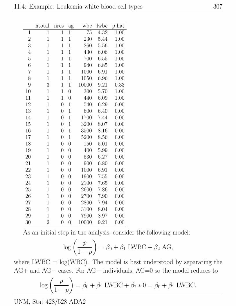
The researchers are interested in modelling the probability p of surviving at
least one year as a function of WBC and AG. They believe that WBC should
be transformed to a log scale, given the skewness in the WBC values.#### Example: Leukemia
## Leukemia white blood cell types example
# ntotal = number of patients with IAG and WBC combination
# nres = number surviving at least one year
# ag = 1 for AG+, 0 for AG-
# wbc = white cell blood count
# lwbc = log white cell blood count
# p.hat = Emperical Probability
leuk <- read.table("http://statacumen.com/teach/ADA2/ADA2_notes_Ch11_leuk.dat"
, header = TRUE)
leuk$ag <- factor(leuk$ag)
leuk$lwbc <- log(leuk$wbc)
leuk$p.hat <- leuk$nres / leuk$ntotal
str(leuk)
## 'data.frame': 30 obs. of 6 variables:
## $ ntotal: int 1 1 1 1 1 1 1 1 3 1 ...
## $ nres : int 1 1 1 1 1 1 1 1 1 1 ...
## $ ag : Factor w/ 2 levels "0","1": 2 2 2 2 2 2 2 2 2 1 ...
## $ wbc : int 75 230 260 430 700 940 1000 1050 10000 300 ...
## $ lwbc : num 4.32 5.44 5.56 6.06 6.55 ...
## $ p.hat : num 1 1 1 1 1 ...
Prof. Erik B. Erhardt
11.4: Example: Leukemia white blood cell types 307
ntotal nres ag wbc lwbc p.hat1 1 1 1 75 4.32 1.002 1 1 1 230 5.44 1.003 1 1 1 260 5.56 1.004 1 1 1 430 6.06 1.005 1 1 1 700 6.55 1.006 1 1 1 940 6.85 1.007 1 1 1 1000 6.91 1.008 1 1 1 1050 6.96 1.009 3 1 1 10000 9.21 0.33
10 1 1 0 300 5.70 1.0011 1 1 0 440 6.09 1.0012 1 0 1 540 6.29 0.0013 1 0 1 600 6.40 0.0014 1 0 1 1700 7.44 0.0015 1 0 1 3200 8.07 0.0016 1 0 1 3500 8.16 0.0017 1 0 1 5200 8.56 0.0018 1 0 0 150 5.01 0.0019 1 0 0 400 5.99 0.0020 1 0 0 530 6.27 0.0021 1 0 0 900 6.80 0.0022 1 0 0 1000 6.91 0.0023 1 0 0 1900 7.55 0.0024 1 0 0 2100 7.65 0.0025 1 0 0 2600 7.86 0.0026 1 0 0 2700 7.90 0.0027 1 0 0 2800 7.94 0.0028 1 0 0 3100 8.04 0.0029 1 0 0 7900 8.97 0.0030 2 0 0 10000 9.21 0.00
As an initial step in the analysis, consider the following model:
log
(p
1− p
)= β0 + β1 LWBC + β2 AG,
where LWBC = log(WBC). The model is best understood by separating the
AG+ and AG− cases. For AG− individuals, AG=0 so the model reduces to
log
(p
1− p
)= β0 + β1 LWBC + β2 ∗ 0 = β0 + β1 LWBC.
UNM, Stat 428/528 ADA2

308 Ch 11: Logistic Regression
For AG+ individuals, AG=1 and the model implies
log
(p
1− p
)= β0 + β1 LWBC + β2 ∗ 1 = (β0 + β2) + β1 LWBC.
The model without AG (i.e., β2 = 0) is a simple logistic model where the
log-odds of surviving one year is linearly related to LWBC, and is independent
of AG. The reduced model with β2 = 0 implies that there is no effect of the
AG level on the survival probability once LWBC has been taken into account.
Including the binary predictor AG in the model implies that there is
a linear relationship between the log-odds of surviving one year and LWBC,
with a constant slope for the two AG levels. This model includes an effect for
the AG morphological factor, but more general models are possible. A natural
extension would be to include a product or interaction effect, a point that I will
return to momentarily.
The parameters are easily interpreted: β0 and β0 + β2 are intercepts for
the population logistic regression lines for AG− and AG+, respectively. The
lines have a common slope, β1. The β2 coefficient for the AG indicator is the
difference between intercepts for the AG+ and AG− regression lines. A picture
of the assumed relationship is given below for β1 < 0. The population regression
lines are parallel on the logit scale only, but the order between AG groups is
preserved on the probability scale.
Prof. Erik B. Erhardt

11.4: Example: Leukemia white blood cell types 309
LWBC
Log-
Odd
s
-5 0 5
-10
-50
5
IAG=1
IAG=0
Logit Scale
LWBC
Pro
babi
lity
-5 0 5
0.0
0.2
0.4
0.6
0.8
1.0
IAG=0
IAG=1
Probability Scale
Before looking at output for the equal slopes model, note that the data
set has 30 distinct AG and LWBC combinations, or 30 “groups” or samples.
Only two samples have more than 1 observation. The majority of the observed
proportions surviving at least one year (number surviving ≥ 1 year/group
sample size) are 0 (i.e., 0/1) or 1 (i.e., 1/1). This sparseness of the data makes
it difficult to graphically assess the suitability of the logistic model (because
the estimated proportions are almost all 0 or 1). Although significance tests
on the regression coefficients do not require large group sizes, the chi-squared
approximation to the deviance statistic is suspect in sparse data settings. With
small group sizes as we have here, most researchers would not interpret the
p-value for D literally. Instead, they would use the p-values to informally check
the fit of the model. Diagnostics would be used to highlight problems with the
model.glm.i.l <- glm(cbind(nres, ntotal - nres) ~ ag + lwbc, family = binomial, leuk)
# Test residual deviance for lack-of-fit (if > 0.10, little-to-no lack-of-fit)
dev.p.val <- 1 - pchisq(glm.i.l$deviance, glm.i.l$df.residual)
dev.p.val
UNM, Stat 428/528 ADA2
310 Ch 11: Logistic Regression
## [1] 0.6842804
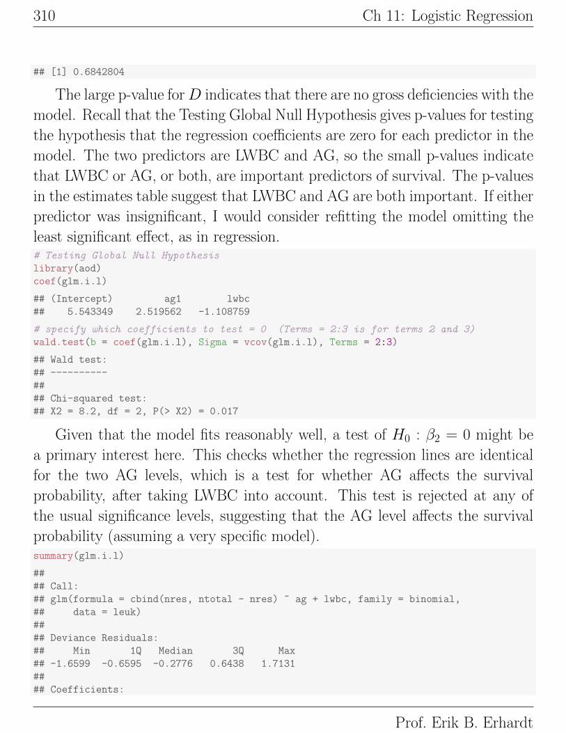
The large p-value forD indicates that there are no gross deficiencies with the
model. Recall that the Testing Global Null Hypothesis gives p-values for testing
the hypothesis that the regression coefficients are zero for each predictor in the
model. The two predictors are LWBC and AG, so the small p-values indicate
that LWBC or AG, or both, are important predictors of survival. The p-values
in the estimates table suggest that LWBC and AG are both important. If either
predictor was insignificant, I would consider refitting the model omitting the
least significant effect, as in regression.# Testing Global Null Hypothesis
library(aod)
coef(glm.i.l)
## (Intercept) ag1 lwbc
## 5.543349 2.519562 -1.108759
# specify which coefficients to test = 0 (Terms = 2:3 is for terms 2 and 3)
wald.test(b = coef(glm.i.l), Sigma = vcov(glm.i.l), Terms = 2:3)
## Wald test:
## ----------
##
## Chi-squared test:
## X2 = 8.2, df = 2, P(> X2) = 0.017
Given that the model fits reasonably well, a test of H0 : β2 = 0 might be
a primary interest here. This checks whether the regression lines are identical
for the two AG levels, which is a test for whether AG affects the survival
probability, after taking LWBC into account. This test is rejected at any of
the usual significance levels, suggesting that the AG level affects the survival
probability (assuming a very specific model).summary(glm.i.l)
##
## Call:
## glm(formula = cbind(nres, ntotal - nres) ~ ag + lwbc, family = binomial,
## data = leuk)
##
## Deviance Residuals:
## Min 1Q Median 3Q Max
## -1.6599 -0.6595 -0.2776 0.6438 1.7131
##
## Coefficients:
Prof. Erik B. Erhardt
11.4: Example: Leukemia white blood cell types 311
## Estimate Std. Error z value Pr(>|z|)
## (Intercept) 5.5433 3.0224 1.834 0.0666 .
## ag1 2.5196 1.0907 2.310 0.0209 *
## lwbc -1.1088 0.4609 -2.405 0.0162 *
## ---
## Signif. codes: 0 '***' 0.001 '**' 0.01 '*' 0.05 '.' 0.1 ' ' 1
##
## (Dispersion parameter for binomial family taken to be 1)
##
## Null deviance: 38.191 on 29 degrees of freedom
## Residual deviance: 23.014 on 27 degrees of freedom
## AIC: 30.635
##
## Number of Fisher Scoring iterations: 5
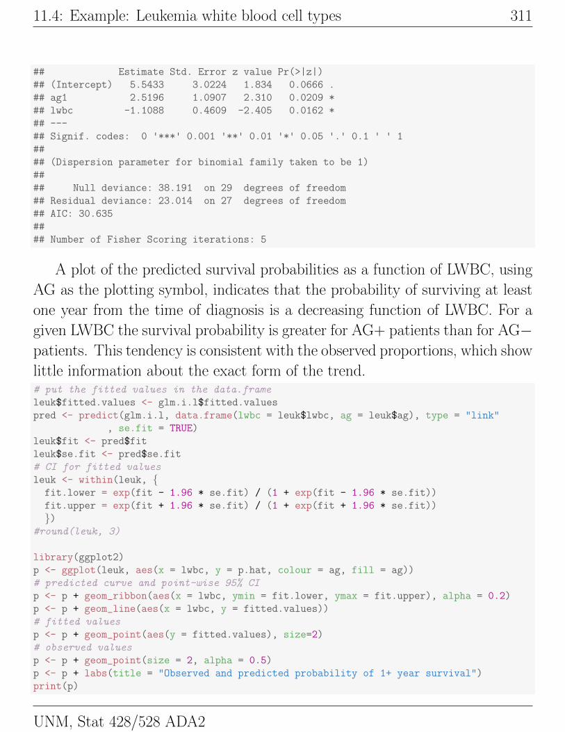
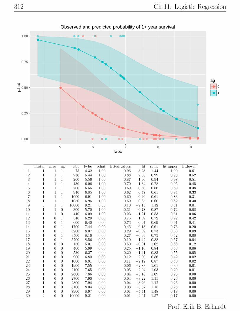
A plot of the predicted survival probabilities as a function of LWBC, using
AG as the plotting symbol, indicates that the probability of surviving at least
one year from the time of diagnosis is a decreasing function of LWBC. For a
given LWBC the survival probability is greater for AG+ patients than for AG−patients. This tendency is consistent with the observed proportions, which show
little information about the exact form of the trend.# put the fitted values in the data.frame
leuk$fitted.values <- glm.i.l$fitted.values
pred <- predict(glm.i.l, data.frame(lwbc = leuk$lwbc, ag = leuk$ag), type = "link"
, se.fit = TRUE)
leuk$fit <- pred$fit
leuk$se.fit <- pred$se.fit
# CI for fitted values
leuk <- within(leuk, {fit.lower = exp(fit - 1.96 * se.fit) / (1 + exp(fit - 1.96 * se.fit))
fit.upper = exp(fit + 1.96 * se.fit) / (1 + exp(fit + 1.96 * se.fit))
})#round(leuk, 3)
library(ggplot2)
p <- ggplot(leuk, aes(x = lwbc, y = p.hat, colour = ag, fill = ag))
# predicted curve and point-wise 95% CI
p <- p + geom_ribbon(aes(x = lwbc, ymin = fit.lower, ymax = fit.upper), alpha = 0.2)
p <- p + geom_line(aes(x = lwbc, y = fitted.values))
# fitted values
p <- p + geom_point(aes(y = fitted.values), size=2)
# observed values
p <- p + geom_point(size = 2, alpha = 0.5)
p <- p + labs(title = "Observed and predicted probability of 1+ year survival")
print(p)
UNM, Stat 428/528 ADA2
312 Ch 11: Logistic Regression
●
●●
●
●
●●
●
●
●
●
●●
●
●●
●
●
●
●
● ●
● ● ●●● ●● ●0.00
0.25
0.50
0.75
1.00
5 6 7 8 9lwbc
p.ha
t
ag●
●
0
1
Observed and predicted probability of 1+ year survival
ntotal nres ag wbc lwbc p.hat fitted.values fit se.fit fit.upper fit.lower1 1 1 1 75 4.32 1.00 0.96 3.28 1.44 1.00 0.612 1 1 1 230 5.44 1.00 0.88 2.03 0.99 0.98 0.523 1 1 1 260 5.56 1.00 0.87 1.90 0.94 0.98 0.514 1 1 1 430 6.06 1.00 0.79 1.34 0.78 0.95 0.455 1 1 1 700 6.55 1.00 0.69 0.80 0.66 0.89 0.386 1 1 1 940 6.85 1.00 0.62 0.47 0.61 0.84 0.337 1 1 1 1000 6.91 1.00 0.60 0.40 0.61 0.83 0.318 1 1 1 1050 6.96 1.00 0.59 0.35 0.60 0.82 0.309 3 1 1 10000 9.21 0.33 0.10 −2.15 1.12 0.51 0.01
10 1 1 0 300 5.70 1.00 0.31 −0.78 0.87 0.72 0.0811 1 1 0 440 6.09 1.00 0.23 −1.21 0.83 0.61 0.0612 1 0 1 540 6.29 0.00 0.75 1.09 0.72 0.92 0.4213 1 0 1 600 6.40 0.00 0.73 0.97 0.69 0.91 0.4114 1 0 1 1700 7.44 0.00 0.45 −0.18 0.61 0.73 0.2015 1 0 1 3200 8.07 0.00 0.29 −0.89 0.73 0.63 0.0916 1 0 1 3500 8.16 0.00 0.27 −0.99 0.75 0.62 0.0817 1 0 1 5200 8.56 0.00 0.19 −1.42 0.88 0.57 0.0418 1 0 0 150 5.01 0.00 0.50 −0.01 1.02 0.88 0.1219 1 0 0 400 5.99 0.00 0.25 −1.10 0.84 0.63 0.0620 1 0 0 530 6.27 0.00 0.20 −1.41 0.83 0.55 0.0521 1 0 0 900 6.80 0.00 0.12 −2.00 0.86 0.42 0.0222 1 0 0 1000 6.91 0.00 0.11 −2.12 0.87 0.40 0.0223 1 0 0 1900 7.55 0.00 0.06 −2.83 1.01 0.30 0.0124 1 0 0 2100 7.65 0.00 0.05 −2.94 1.03 0.29 0.0125 1 0 0 2600 7.86 0.00 0.04 −3.18 1.09 0.26 0.0026 1 0 0 2700 7.90 0.00 0.04 −3.22 1.11 0.26 0.0027 1 0 0 2800 7.94 0.00 0.04 −3.26 1.12 0.26 0.0028 1 0 0 3100 8.04 0.00 0.03 −3.37 1.15 0.25 0.0029 1 0 0 7900 8.97 0.00 0.01 −4.41 1.48 0.18 0.0030 2 0 0 10000 9.21 0.00 0.01 −4.67 1.57 0.17 0.00
Prof. Erik B. Erhardt
11.4: Example: Leukemia white blood cell types 313
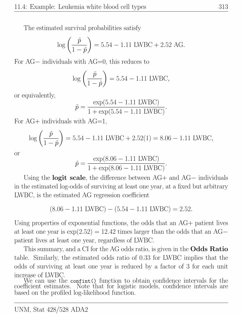
The estimated survival probabilities satisfy
log
(p̃
1− p̃
)= 5.54− 1.11 LWBC + 2.52 AG.
For AG− individuals with AG=0, this reduces to
log
(p̃
1− p̃
)= 5.54− 1.11 LWBC,
or equivalently,
p̃ =exp(5.54− 1.11 LWBC)
1 + exp(5.54− 1.11 LWBC).
For AG+ individuals with AG=1,
log
(p̃
1− p̃
)= 5.54− 1.11 LWBC + 2.52(1) = 8.06− 1.11 LWBC,
or
p̃ =exp(8.06− 1.11 LWBC)
1 + exp(8.06− 1.11 LWBC).
Using the logit scale, the difference between AG+ and AG− individuals
in the estimated log-odds of surviving at least one year, at a fixed but arbitrary
LWBC, is the estimated AG regression coefficient
(8.06− 1.11 LWBC)− (5.54− 1.11 LWBC) = 2.52.
Using properties of exponential functions, the odds that an AG+ patient lives
at least one year is exp(2.52) = 12.42 times larger than the odds that an AG−patient lives at least one year, regardless of LWBC.
This summary, and a CI for the AG odds ratio, is given in the Odds Ratio
table. Similarly, the estimated odds ratio of 0.33 for LWBC implies that the
odds of surviving at least one year is reduced by a factor of 3 for each unit
increase of LWBC.We can use the confint() function to obtain confidence intervals for the
coefficient estimates. Note that for logistic models, confidence intervals arebased on the profiled log-likelihood function.
UNM, Stat 428/528 ADA2

314 Ch 11: Logistic Regression
## CIs using profiled log-likelihood
confint(glm.i.l)
## Waiting for profiling to be done...
## 2.5 % 97.5 %
## (Intercept) 0.1596372 12.4524409
## ag1 0.5993391 5.0149271
## lwbc -2.2072275 -0.3319512
We can also get CIs based on just the standard errors by using the defaultmethod.## CIs using standard errors
confint.default(glm.i.l)
## 2.5 % 97.5 %
## (Intercept) -0.3804137 11.467112
## ag1 0.3818885 4.657236
## lwbc -2.0121879 -0.205330
You can also exponentiate the coefficients and confidence interval boundsand interpret them as odds-ratios.## coefficients and 95% CI
cbind(OR = coef(glm.i.l), confint(glm.i.l))
## Waiting for profiling to be done...
## OR 2.5 % 97.5 %
## (Intercept) 5.543349 0.1596372 12.4524409
## ag1 2.519562 0.5993391 5.0149271
## lwbc -1.108759 -2.2072275 -0.3319512
## odds ratios and 95% CI
exp(cbind(OR = coef(glm.i.l), confint(glm.i.l)))
## Waiting for profiling to be done...
## OR 2.5 % 97.5 %
## (Intercept) 255.5323676 1.1730851 2.558741e+05
## ag1 12.4231582 1.8209149 1.506452e+02
## lwbc 0.3299682 0.1100052 7.175224e-01
Although the equal slopes model appears to fit well, a more general model
might fit better. A natural generalization here would be to add an interaction,
or product term, AG × LWBC to the model. The logistic model with an AG
effect and the AG× LWBC interaction is equivalent to fitting separate logistic
regression lines to the two AG groups. This interaction model provides an easy
way to test whether the slopes are equal across AG levels. I will note that the
interaction term is not needed here.
Prof. Erik B. Erhardt
11.4: Example: Leukemia white blood cell types 315
Interpretting odds ratios in logistic regression Let’s begin with
probability3. Let’s say that the probability of success is 0.8, thus p = 0.8.
Then the probability of failure is q = 1 − p = 0.2. The odds of success are
defined as odds(success) = p/q = 0.8/0.2 = 4, that is, the odds of success are
4 to 1. The odds of failure would be odds(failure) = q/p = 0.2/0.8 = 0.25,
that is, the odds of failure are 1 to 4. Next, let’s compute the odds ratio
by OR = odds(success)/odds(failure) = 4/0.25 = 16. The interpretation of
this odds ratio would be that the odds of success are 16 times greater than
for failure. Now if we had formed the odds ratio the other way around with
odds of failure in the numerator, we would have gotten something like this,
OR = odds(failure)/odds(success) = 0.25/4 = 0.0625.
Another example This example is adapted from Pedhazur (1997). Sup-
pose that seven out of 10 males are admitted to an engineering school while
three of 10 females are admitted. The probabilities for admitting a male are,
p = 7/10 = 0.7 and q = 1 − 0.7 = 0.3. Here are the same probabilities
for females, p = 3/10 = 0.3 and q = 1 − 0.3 = 0.7. Now we can use
the probabilities to compute the admission odds for both males and females,
odds(male) = 0.7/0.3 = 2.33333 and odds(female) = 0.3/0.7 = 0.42857. Next,
we compute the odds ratio for admission, OR = 2.3333/0.42857 = 5.44. Thus,
the odds of a male being admitted are 5.44 times greater than for a female.
Leukemia example In the example above, the OR of surviving at least
one year increases 12.43 times for AG+ vs AG−, and increases 0.33 times
(that’s a decrease) for every unit increase in lwbc.
Example: Mortality of confused flour beetles This example illus-
trates a quadratic logistic model.
3Borrowed graciously from UCLA Academic Technology Services at http://www.ats.ucla.edu/stat/sas/faq/oratio.htm
UNM, Stat 428/528 ADA2
316 Ch 11: Logistic Regression
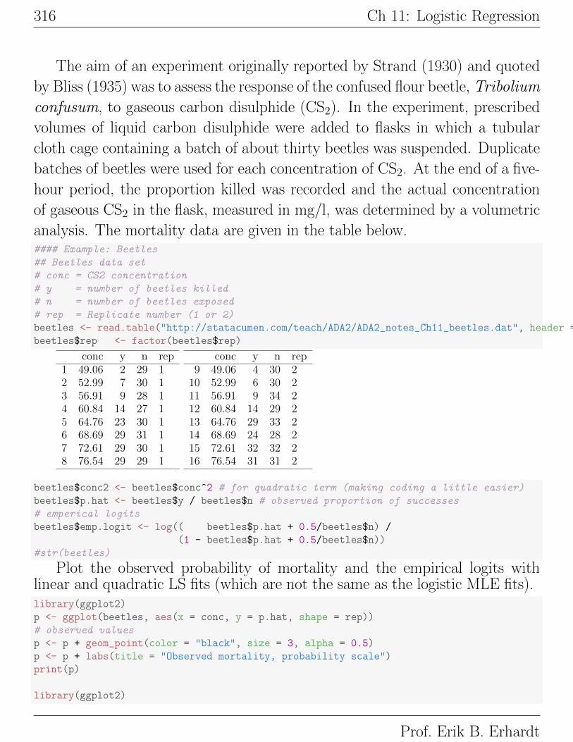
The aim of an experiment originally reported by Strand (1930) and quoted
by Bliss (1935) was to assess the response of the confused flour beetle, Tribolium
confusum, to gaseous carbon disulphide (CS2). In the experiment, prescribed
volumes of liquid carbon disulphide were added to flasks in which a tubular
cloth cage containing a batch of about thirty beetles was suspended. Duplicate
batches of beetles were used for each concentration of CS2. At the end of a five-
hour period, the proportion killed was recorded and the actual concentration
of gaseous CS2 in the flask, measured in mg/l, was determined by a volumetric
analysis. The mortality data are given in the table below.#### Example: Beetles
## Beetles data set
# conc = CS2 concentration
# y = number of beetles killed
# n = number of beetles exposed
# rep = Replicate number (1 or 2)
beetles <- read.table("http://statacumen.com/teach/ADA2/ADA2_notes_Ch11_beetles.dat", header = TRUE)
beetles$rep <- factor(beetles$rep)
conc y n rep1 49.06 2 29 12 52.99 7 30 13 56.91 9 28 14 60.84 14 27 15 64.76 23 30 16 68.69 29 31 17 72.61 29 30 18 76.54 29 29 1
conc y n rep9 49.06 4 30 2
10 52.99 6 30 211 56.91 9 34 212 60.84 14 29 213 64.76 29 33 214 68.69 24 28 215 72.61 32 32 216 76.54 31 31 2
beetles$conc2 <- beetles$conc^2 # for quadratic term (making coding a little easier)
beetles$p.hat <- beetles$y / beetles$n # observed proportion of successes
# emperical logits
beetles$emp.logit <- log(( beetles$p.hat + 0.5/beetles$n) /
(1 - beetles$p.hat + 0.5/beetles$n))
#str(beetles)
Plot the observed probability of mortality and the empirical logits withlinear and quadratic LS fits (which are not the same as the logistic MLE fits).library(ggplot2)
p <- ggplot(beetles, aes(x = conc, y = p.hat, shape = rep))
# observed values
p <- p + geom_point(color = "black", size = 3, alpha = 0.5)
p <- p + labs(title = "Observed mortality, probability scale")
print(p)
library(ggplot2)
Prof. Erik B. Erhardt
11.4: Example: Leukemia white blood cell types 317
p <- ggplot(beetles, aes(x = conc, y = emp.logit))
p <- p + geom_smooth(method = "lm", colour = "red", se = FALSE)
p <- p + geom_smooth(method = "lm", formula = y ~ poly(x, 2), colour = "blue", se = FALSE)
# observed values
p <- p + geom_point(aes(shape = rep), color = "black", size = 3, alpha = 0.5)
p <- p + labs(title = "Empirical logit with `naive' LS fits (not MLE)")
print(p)
0.25
0.50
0.75
1.00
50 60 70conc
p.ha
t
rep
1
2
Observed mortality, probability scale
−2
0
2
4
50 60 70conc
emp.
logi
t rep
1
2
Empirical logit with `naive' LS fits (not MLE)
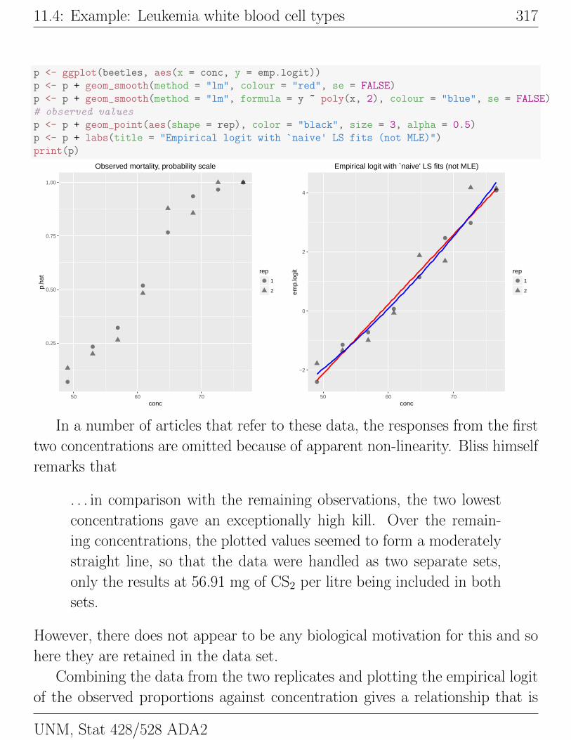
In a number of articles that refer to these data, the responses from the first
two concentrations are omitted because of apparent non-linearity. Bliss himself
remarks that
. . . in comparison with the remaining observations, the two lowest
concentrations gave an exceptionally high kill. Over the remain-
ing concentrations, the plotted values seemed to form a moderately
straight line, so that the data were handled as two separate sets,
only the results at 56.91 mg of CS2 per litre being included in both
sets.
However, there does not appear to be any biological motivation for this and so
here they are retained in the data set.
Combining the data from the two replicates and plotting the empirical logit
of the observed proportions against concentration gives a relationship that is
UNM, Stat 428/528 ADA2

318 Ch 11: Logistic Regression
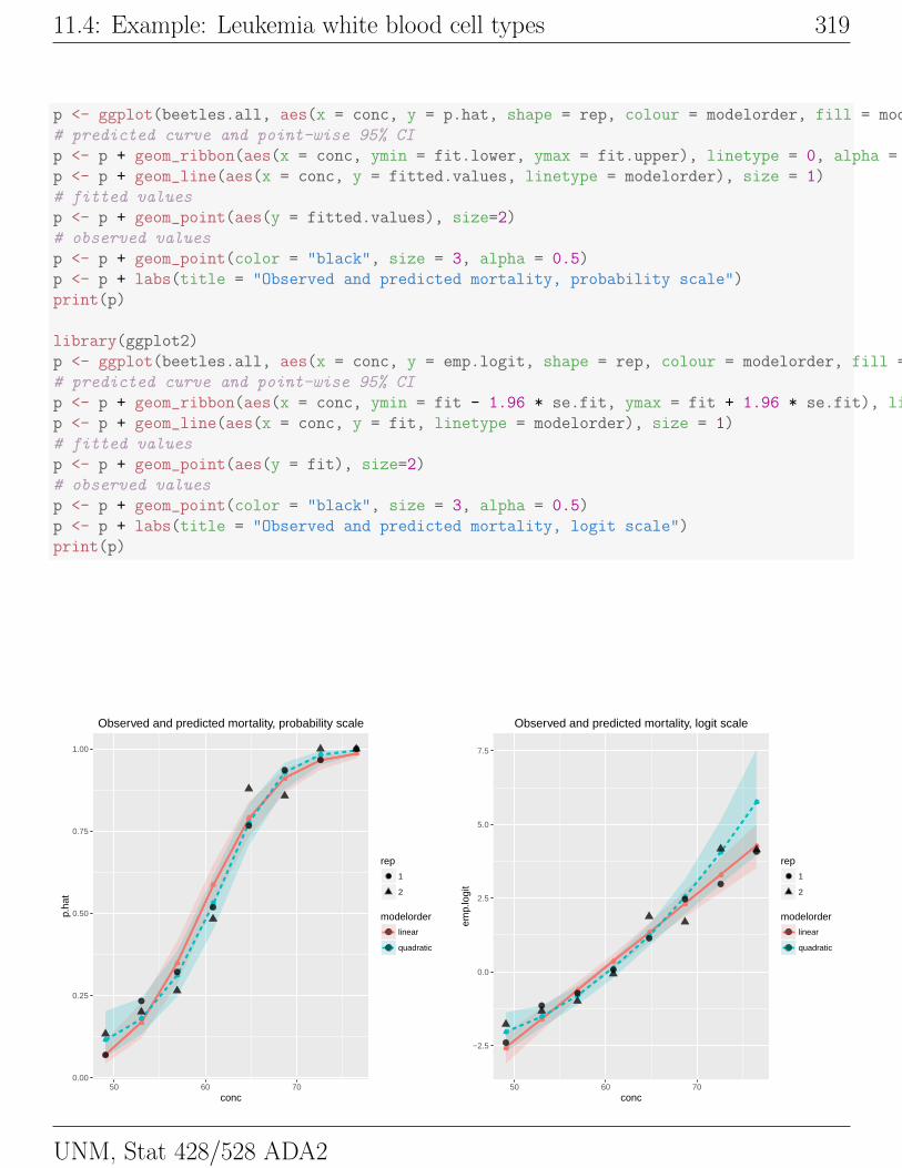
better fit by a quadratic than a linear relationship,
log
(p
1− p
)= β0 + β1X + β2X
2.
The right plot below shows the linear and quadratic model fits to the observed
values with point-wise 95% confidence bands on the logit scale, and on the left
is the same on the proportion scale.# fit logistic regression to create lines on plots below
# linear
glm.beetles1 <- glm(cbind(y, n - y) ~ conc, family = binomial, beetles)
# quadratic
glm.beetles2 <- glm(cbind(y, n - y) ~ conc + conc2, family = binomial, beetles)
## put model fits for two models together
beetles1 <- beetles
# put the fitted values in the data.frame
beetles1$fitted.values <- glm.beetles1$fitted.values
pred <- predict(glm.beetles1, data.frame(conc = beetles1$conc), type = "link", se.fit = TRUE) #£
beetles1$fit <- pred$fit
beetles1$se.fit <- pred$se.fit
# CI for fitted values
beetles1 <- within(beetles1, {fit.lower = exp(fit - 1.96 * se.fit) / (1 + exp(fit - 1.96 * se.fit))
fit.upper = exp(fit + 1.96 * se.fit) / (1 + exp(fit + 1.96 * se.fit))
})beetles1$modelorder <- "linear"
beetles2 <- beetles
# put the fitted values in the data.frame
beetles2$fitted.values <- glm.beetles2$fitted.values
pred <- predict(glm.beetles2, data.frame(conc = beetles2$conc, conc2 = beetles2$conc2), type = "link", se.fit = TRUE)
beetles2$fit <- pred$fit
beetles2$se.fit <- pred$se.fit
# CI for fitted values
beetles2 <- within(beetles2, {fit.lower = exp(fit - 1.96 * se.fit) / (1 + exp(fit - 1.96 * se.fit))
fit.upper = exp(fit + 1.96 * se.fit) / (1 + exp(fit + 1.96 * se.fit))
})beetles2$modelorder <- "quadratic"
beetles.all <- rbind(beetles1, beetles2)
beetles.all$modelorder <- factor(beetles.all$modelorder)
# plot on logit and probability scales
library(ggplot2)
Prof. Erik B. Erhardt
11.4: Example: Leukemia white blood cell types 319
p <- ggplot(beetles.all, aes(x = conc, y = p.hat, shape = rep, colour = modelorder, fill = modelorder))
# predicted curve and point-wise 95% CI
p <- p + geom_ribbon(aes(x = conc, ymin = fit.lower, ymax = fit.upper), linetype = 0, alpha = 0.1)
p <- p + geom_line(aes(x = conc, y = fitted.values, linetype = modelorder), size = 1)
# fitted values
p <- p + geom_point(aes(y = fitted.values), size=2)
# observed values
p <- p + geom_point(color = "black", size = 3, alpha = 0.5)
p <- p + labs(title = "Observed and predicted mortality, probability scale")
print(p)
library(ggplot2)
p <- ggplot(beetles.all, aes(x = conc, y = emp.logit, shape = rep, colour = modelorder, fill = modelorder))
# predicted curve and point-wise 95% CI
p <- p + geom_ribbon(aes(x = conc, ymin = fit - 1.96 * se.fit, ymax = fit + 1.96 * se.fit), linetype = 0, alpha = 0.1)
p <- p + geom_line(aes(x = conc, y = fit, linetype = modelorder), size = 1)
# fitted values
p <- p + geom_point(aes(y = fit), size=2)
# observed values
p <- p + geom_point(color = "black", size = 3, alpha = 0.5)
p <- p + labs(title = "Observed and predicted mortality, logit scale")
print(p)
●
●
●
●
●
●
●●
●
●
●
●
●
●
●●
0.00
0.25
0.50
0.75
1.00
50 60 70conc
p.ha
t
rep● 1
2
modelorder●
●
linear
quadratic
Observed and predicted mortality, probability scale
●
●
●
●
●
●
●
●
●
●
●
●
●
●
●
●
−2.5
0.0
2.5
5.0
7.5
50 60 70conc
emp.
logi
t
rep● 1
2
modelorder●
●
linear
quadratic
Observed and predicted mortality, logit scale
UNM, Stat 428/528 ADA2

320 Ch 11: Logistic Regression
11.5 Example: The UNM Trauma Data
The data to be analyzed here were collected on 3132 patients admitted to The
University of New Mexico Trauma Center between the years 1991 and 1994. For
each patient, the attending physician recorded their age, their revised trauma
score (RTS), their injury severity score (ISS), whether their injuries were blunt
(i.e., the result of a car crash: BP=0) or penetrating (i.e., gunshot/knife wounds:
BP=1), and whether they eventually survived their injuries (SURV=0 if not,
SURV=1 if survived). Approximately 10% of patients admitted to the UNM
Trauma Center eventually die from their injuries.
The ISS is an overall index of a patient’s injuries, based on the approximately
1300 injuries cataloged in the Abbreviated Injury Scale. The ISS can take on
values from 0 for a patient with no injuries to 75 for a patient with 3 or more
life threatening injuries. The ISS is the standard injury index used by trauma
centers throughout the U.S. The RTS is an index of physiologic injury, and
is constructed as a weighted average of an incoming patient’s systolic blood
pressure, respiratory rate, and Glasgow Coma Scale. The RTS can take on
values from 0 for a patient with no vital signs to 7.84 for a patient with normal
vital signs.
Champion et al. (1981) proposed a logistic regression model to estimate
the probability of a patient’s survival as a function of RTS, the injury severity
score ISS, and the patient’s age, which is used as a surrogate for physiologic
reserve. Subsequent survival models included the binary effect BP as a means
to differentiate between blunt and penetrating injuries.
We will develop a logistic model for predicting survival from ISS, AGE,
BP, and RTS, and nine body regions. Data on the number of severe injuries
in each of the nine body regions is also included in the database, so we will also
assess whether these features have any predictive power. The following labels
were used to identify the number of severe injuries in the nine regions: AS =
head, BS = face, CS = neck, DS = thorax, ES = abdomen, FS = spine, GS =
upper extremities, HS = lower extremities, and JS = skin.
Prof. Erik B. Erhardt

11.5: Example: The UNM Trauma Data 321
#### Example: UNM Trauma Data
trauma <- read.table("http://statacumen.com/teach/ADA2/ADA2_notes_Ch11_trauma.dat"
, header = TRUE)
## Variables
# surv = survival (1 if survived, 0 if died)
# rts = revised trauma score (range: 0 no vital signs to 7.84 normal vital signs)
# iss = injury severity score (0 no injuries to 75 for 3 or more life threatening injuries)
# bp = blunt or penetrating injuries (e.g., car crash BP=0 vs gunshot/knife wounds BP=1)
# Severe injuries: add the severe injuries 3--6 to make summary variables
trauma <- within(trauma, {as = a3 + a4 + a5 + a6 # as = head
bs = b3 + b4 + b5 + b6 # bs = face
cs = c3 + c4 + c5 + c6 # cs = neck
ds = d3 + d4 + d5 + d6 # ds = thorax
es = e3 + e4 + e5 + e6 # es = abdomen
fs = f3 + f4 + f5 + f6 # fs = spine
gs = g3 + g4 + g5 + g6 # gs = upper extremities
hs = h3 + h4 + h5 + h6 # hs = lower extremities
js = j3 + j4 + j5 + j6 # js = skin
})# keep only columns of interest
names(trauma)
## [1] "id" "surv" "a1" "a2" "a3" "a4" "a5" "a6" "b1" "b2"
## [11] "b3" "b4" "b5" "b6" "c1" "c2" "c3" "c4" "c5" "c6"
## [21] "d1" "d2" "d3" "d4" "d5" "d6" "e1" "e2" "e3" "e4"
## [31] "e5" "e6" "f1" "f2" "f3" "f4" "f5" "f6" "g1" "g2"
## [41] "g3" "g4" "g5" "g6" "h1" "h2" "h3" "h4" "h5" "h6"
## [51] "j1" "j2" "j3" "j4" "j5" "j6" "iss" "iciss" "bp" "rts"
## [61] "age" "prob" "js" "hs" "gs" "fs" "es" "ds" "cs" "bs"
## [71] "as"
trauma <- subset(trauma, select = c(id, surv, as:js, iss:prob))
head(trauma)
## id surv as bs cs ds es fs gs hs js iss iciss bp rts age prob
## 1 1238385 1 0 0 0 1 0 0 0 0 0 13 0.8612883 0 7.8408 13 0.9909890
## 2 1238393 1 0 0 0 0 0 0 0 0 0 5 0.9421876 0 7.8408 23 0.9947165
## 3 1238898 1 0 0 0 0 0 0 2 0 0 13 0.7251130 0 7.8408 43 0.9947165
## 4 1239516 1 1 0 0 0 0 0 0 0 0 16 1.0000000 0 5.9672 17 0.9615540
## 5 1239961 1 1 0 0 0 0 0 0 0 1 9 0.9346634 0 4.8040 20 0.9338096
## 6 1240266 1 0 0 0 0 0 0 0 1 0 13 0.9004691 0 7.8408 32 0.9947165
#str(trauma)
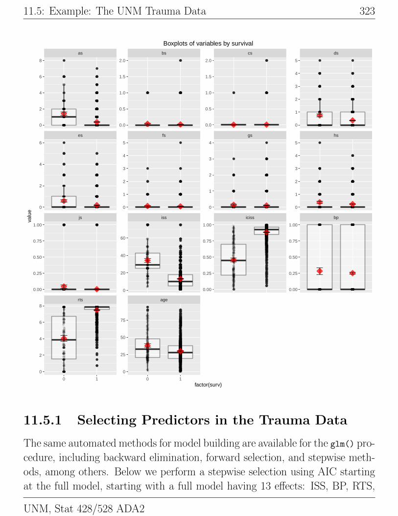
I made side-by-side boxplots of the distributions of ISS, AGE, RTS, and
AS through JS for the survivors and non-survivors. In several body regions
the number of injuries is limited, so these boxplots are not very enlightening.
Survivors tend to have lower ISS scores, tend to be slightly younger, tend to
UNM, Stat 428/528 ADA2

322 Ch 11: Logistic Regression
have higher RTS scores, and tend to have fewer severe head (AS) and abdomen
injuries (ES) than non-survivors. The importance of the effects individually
towards predicting survival is directly related to the separation between the
survivors and non-survivors scores.# Create boxplots for each variable by survival
library(reshape2)
trauma.long <- melt(trauma, id.vars = c("id", "surv", "prob"))
# Plot the data using ggplot
library(ggplot2)
p <- ggplot(trauma.long, aes(x = factor(surv), y = value))
# boxplot, size=.75 to stand out behind CI
p <- p + geom_boxplot(size = 0.75, alpha = 0.5)
# points for observed data
p <- p + geom_point(position = position_jitter(w = 0.05, h = 0), alpha = 0.1)
# diamond at mean for each group
p <- p + stat_summary(fun.y = mean, geom = "point", shape = 18, size = 6,
alpha = 0.75, colour = "red")
# confidence limits based on normal distribution
p <- p + stat_summary(fun.data = "mean_cl_normal", geom = "errorbar",
width = .2, alpha = 0.8)
p <- p + facet_wrap( ~ variable, scales = "free_y", ncol = 4)
p <- p + labs(title = "Boxplots of variables by survival")
print(p)
Prof. Erik B. Erhardt
11.5: Example: The UNM Trauma Data 323
●●●●●
●
●●
●●●●●●
●
●●
●
●
●
●●●●
●
●●●●●●●
●
●●●●●●
●
●●
●●●
●●
●
●
●
●
●
●●
●
●
●●●
●
●
●●●
●
●
●
●
●
●●
●
●
●
●
●●
●●●
●
●
●
●●●
●
●
●
●
●
●●●
●●
●
●
●
●
●●●
●
●
●
●
●
●
●
●
●
●
●
●
●
●●●●
●
●
●
●●
●
●●
●●
●●
●
●●
●
●●
●
●
●
●●
●
●
●
●●
●
●●
●
●
●
●●
●
●●●
●●
●
●●●●●
●
●
●
●●
●
●●●●
●
●
●
●●●●
●
●●●
●
●
●
●
●
●●
●
●
●
●
●
●
●●●
●
●
●
●
●●
●
●●●
●
●
●
●●●
●
●
●
●●●
●
●●●●●●
●
●
●
●
●●
●
●
●
●
●●●●●
●
●
●
●
●
●
●
●●
●
●
●
●
●
●
●●
●
●●●●
●●
●
●●
●
●●
●
●●
●
●
●
●
●●
●
●
●
●●
●
●●
●●
●●●
●
●●
●
●
●
●
●
●
●
●
●
●
●
●
●
●●●
●
●●●●●●●●
●●
●
●●●●
●●●
●
●
●●
●
●
●
●
●
●●
●
●
●
●
●
●●
●●
●
●●
●
●
●
●
●
●
●
●
●
●
●
●
●●
●
●●●
●
●●●●●
●
●
●
●
●●
●●●
●
●●
●
●
●
●●
●
●●
●●
●
●●
●
●
●
●
●●●●
●
●
●
●●
●
●
●
●
●
●
●●
●●●
●
●
●
●
●
●●●
●
●
●
●
●●
●●●
●
●
●
●
●●
●
●●
●
●●
●●
●
●
●●●
●
●
●
●●
●●
●
●
●
●
●●
●
●●●●
●
●●●
●
●
●
●●
●●
●●●●
●
●●●●●●
●
●●●
●
●
●
●●●
●●
●
●●●●
●
●
●
●
●
●
●●
●
●
●
●
●
●
●
●●●●
●●
●
●
●
●
●
●
●●
●
●
●
●
●
●
●
●●
●
●●●
●
●●●
●
●●●●●●●●●● ●●●●●●●●
●
●●●●●●●●●●●●●●
●
●●●●●●●●●●●●●●●●●●●●●●●●●●●● ●● ●●
●
●
●
●●●●●●●●●
●
●●●●●●●●●
●
●
●●●
●
●
●
●●●●●
●●
●
●
●
●
●
●● ●●●●
●
●●●●●●●●●●●●
●
●●●●●
●●
●●●●●●●●●●●●●●●●●●●
●
●
●
●●●
●
●●
●
●
●
●
●●●
●
●
●
●
●
●
●●●●●
●
●
●
●●●
●
●●
●
●
●
●
●●●
●
●●●●●●●●●●●●
●
●●●●●
●
●●●
●
●●●
●
●
●
●●●●
●
●
●
●●●●
●●
●
●●
●
●●●●●●●●●
●
●
●
●
●●●●●●●
●
●
●
●●
●
●●●
●
●
●
●●●●●
●
●●●
●
●●●●●●
●
●
●
●
●
●●●
●
●
●●
●
●
●
●
●●
●
●●
●
●●●●●
●●
●
●
●
●
●
●●●●●●●●
●
●
●
●●●
●
●●●●●●●●●●●●●
●
●
●
●
●
●
●
●●●●●●
●●●
●●
●●
●
●●
●
●
●
●●
●
●●●●
●
●●●
●●
●
●
●
●
●
●
●
●●●
●
●●●●
●●
●●
●●●
●
●●●●●●●●
●
●●●●●
●
●●
●
●
●
●●●●
●
●●
●
●●●
●●
●
●
●
●
●
●●●
●
●●
●●
●
●
●
●●●●●●●●●
●
●●
●
●●●
●●
●
●
●
●
●
●●
●
●
●●
●●
●
●
●
●●
●
●
●●
●
●●●
●
●
●
●●●●
●
●●●●●●●●●●●
●
●
●●
●
●
●●●
●●
●●
●●
●
●●
●
●●●●●●●●●●●●
●
●
●
●●
●
●
●
●●● ●●●
●
●●●●●●●●●●●●●
●
●
●●●
●●●●●●●●●●●●●●●●●●●●●●●●●●●●●●●●●●●●●●●●●●●●●
●
●●●●●●●●●●
●
●●●●●●●●●●●●●●●
●
●●●●●●●●●●
●
●●●●
●
●●●
●
●●●●●●●●
●
●●●●●●
●
●
●
●●●
●
●●●●●●●●●●●●
●
●●●●●●●
●
●
●
●●●●●●
●●●●
●●●●
●●●●●●●
●
●●
●
●●●●●
●●●●
●●
●●●●●
●
●
●●●●
●
●
●●
●●●●●●●●
●●
●●●●
●
●●
●●
●
●●
●
●●●●●●●●●
●
●●
●
●
●
●●●
●
●●●●●●
●
●
●
●●
●
●
●●
●
●
●●
●●●
●●●●
●
●●●●●
●
●
●
●●●●●
●●
●●●●●
●
●●
●
●●
●
●●●●●●
●●
●●●●●
●
●●●
●
●
●
●
●
●●●
●
●●
●
●●●
●
●●
●
●●●●●●
●
●●●●●
●
●●●●●●●●●●●●●●●●
●
●
●
●●●●●●●●●●●●
●
●
●
●
●
●
●
●●●●●
●
●
●
●●
●
●
●●
●●
●
●
●●●●●
●
●
●●
●●
●●
●
●●
●●
●
●●
●
●
●●●●
●●
●
●
●
●●
●●
●
●
●
●●
●
●
●
●●
●
●
●
●●●●
●●
●●●
●
●
●●●●●
●
●●
●●
●
●
●●●●●
●
● ●●●●●●●●●●●●●●
●
●●●●●●●●●
●
●
●●
●
●●●●
●
●
●
●●
●
●
●
●
●●●●●●
●
●
●
●●
●
●
●
●
●●●
●
●●
●
●
●●
●
●●●●
●
●●
●
●
●●
●
●●
●
●
●
●●
●●●
●
●
●●●●●
●
●
●●
●●
●
●
●●
●
●
●
●
●
●
●
●
●●
●
●●●
●
●●●●●
●
●●●●
●●
●●●●●●●●●●●●●●●●
●
●●●●●
●
●●
●
●●●●●●●
●
●●
●
●●●
●
●●●
●
●●●●●
●
●
●
●●●
●●
●●
●
●●●●●
●
●●
●
●●●●●●
●
●
●●
●
●●●●
●
●●●
●
●
●
●
●
●●
●
●
●●
●●●●●●●●●●●
●
●
●
●
●●●
●●●
●
●●●●●●●●
●
●●●●●●●●
●
●●●●●●●●●
●
●●●●●●●●●●●●●●●●●●
●
●●●
●
●
●
●●
●
●
●●
●
●●
●
●●
●●
●●
●
●●
●
●
●●●●
●●
●
●
●
●●
●
●●
●
●
●●●●
●
●●●●
●●
●●●●
●
●●
●
●●●●●●
●
●●●●
●
●●
●
●●●
●
●●●●●●●●●●●●●●●●●●
●
●●
●
●
●●●
●
●●●●●●●●●●
●
●●●●●
●
●●
●
●●
●
●
●
●●
●
●●●●●
●
●●●
●
●●
●
●●●●●
●
●●●●
●
●●●
●
●
●●●●
●
●
●
●●●●●
●
●●●●●●●●
●
●●●●●
●
●●●●
●
●●
●●
●
●●
●●●●●
●
●
●●
●
●●
●●●●
●
●
●
●●●●●●●●●●●● ●●●●●●●●●●● ●●●●●●●●●●●●●●●●●●●●●●●●●●
●●●●●●
●
●
●●●●
●
●
●●●
●
●
●
●
●●
●●●●
●
●
●
●
●
●
●
●●●●
●●
●
●
●
●
●●
●●
●
●
●
●
●
●
●●●●
●
●
●
●
●
●●
●
●
●●
●
●
●
●
●
●
●
●●●●●
●
●
●
●
●●
●
●
●
●
●
●●
●
●
●
●●
●
●
●
●
●
●
●
●
●
●●
●
●●
●
●●
●
●
●●●●
●
●
●
●●
●
●●
●
●
●
●
●
●
●
●
●
●
●
●
●●
●
●
●
●
●●
●
●
●
●
●●
●
●
●
●●
●
●●●
●●
●
●
●●
●●
●
●
●
●●●
●
●
●
●
●●●
●
●
●
●
●
●
●
●
●
●
●
●
●
●
●
●
●
●
●
●
●
●
●
●
●
●
●●●
●
●
●
●
●
●
●
●
●
●●
●
●●●●
●
●
●
●
●
●●
●
●●●
●
●●
●
●
●●
●
●
●
●
●
●
●
●
●●●●
●
●
●
●
●
●
●●
●
●
●
●
●
●●
●
●
●
●
●●●
●●
●●●
●
●●
●
●
●
●
●
●
●
●
●●●
●●●
●
●
●
●●
●
●
●
●
●
●●
●●
●●
●
●
●
●
●●●
●
●
●
●
●
●
●
●
●●
●
●
●
●
●
●
●
●●
●●●
●
●
●
●●
●
●●●
●
●
●●
●
●
●
●●
●●
●●●
●
●
●●
●
●
●●
●
●
●●●
●
●●
●
●●
●
●
●●
●
●
●
●●
●●
●
●●
●
●
●
●
●
●●●
●
●●●
●
●
●
●
●
●
●●
●
●
●●
●
●
●
●
●
●
●
●
●
●●
●
●
●●●●
●
●
●
●
●●
●
●
●
●
●
●
●
●
●
●
●
●●●
●
●
●●
●
●
●●
●
●●
●●
●
●
●●
●
●
●
●●●●●●
●
●
●
●
●
●●
●
●●●
●
●
●
●
●●
●
●
●●●
●
●●
●
●
●
●
●●
●
●
●●
●
●
●
●
●●
●
●
●
●●●
●
●
●
●
●
●
●●
●●
●
●●●●●
●
●
●
●●
●
●
●
●
●
●●●
●
●●
●
●●●
●
●●●
●
●
●
●
●
●
●
●
●
●●
●●
●
●●
●●●●
●●
●
●
●
●●
●●
●
●●●
●●●●
●
●
●
●
●
●
●
●●
●●
●
●
●
●●
●
●
●
●
●
●●●
●
●
●●●
●
●●●
●
●
●
●
●
●●
●
●
●
●
●
●
●
●
●
●
●
●●
●
●
●
●
●
●
●
●
●
●
●
●
●
●
●●
●●
●
●●
●
●
●
●●
●
●
●
●
●
●
●
●●
●●
●
●●
●
●
●
●
●
●
●
●
●
●
●
●●
●
●
●●
●●
●●
●
●
●
●
●
●●
●
●
●
●
●
●
●
●
●
●
●
●
●
●
●●
●
●
●
●●●●
●●●
●
●
●
●
●
●
●
●
●
●●
●
●
●
●
●
●●
●
●●
●
●●●●
●
●
●●
●●
●●
●●
●
●
●
●●
●
●
●
●
●●●●
●●●●●
●
●
●●●
●●
●●●
●
●
●
●
●
●
●●●●●
●●●●●
●
●●●●●
●
●●●
●
●
●
●●
●
●
●
●
●
●
●
●●
●
●
●●
●
●
●●
●
●
●●●●●●
as bs cs ds
es fs gs hs
js iss iciss bp
rts age
0
2
4
6
8
0.0
0.5
1.0
1.5
2.0
0.0
0.5
1.0
1.5
2.0
0
1
2
3
4
5
0
2
4
6
0
1
2
3
4
5
0
1
2
3
4
0
1
2
3
4
5
0.00
0.25
0.50
0.75
1.00
0
20
40
60
0.00
0.25
0.50
0.75
1.00
0.00
0.25
0.50
0.75
1.00
0
2
4
6
8
0
25
50
75
0 1 0 1factor(surv)
valu
e
Boxplots of variables by survival
11.5.1 Selecting Predictors in the Trauma Data
The same automated methods for model building are available for the glm() pro-
cedure, including backward elimination, forward selection, and stepwise meth-
ods, among others. Below we perform a stepwise selection using AIC starting
at the full model, starting with a full model having 13 effects: ISS, BP, RTS,
UNM, Stat 428/528 ADA2
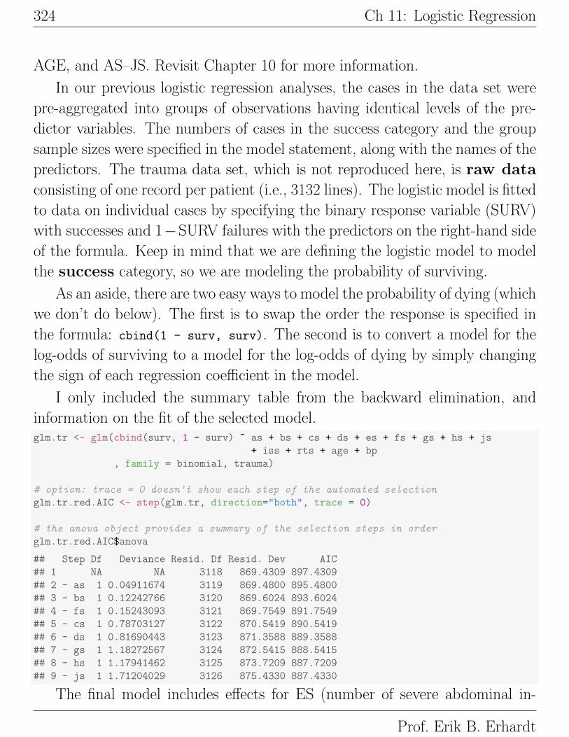
324 Ch 11: Logistic Regression
AGE, and AS–JS. Revisit Chapter 10 for more information.
In our previous logistic regression analyses, the cases in the data set were
pre-aggregated into groups of observations having identical levels of the pre-
dictor variables. The numbers of cases in the success category and the group
sample sizes were specified in the model statement, along with the names of the
predictors. The trauma data set, which is not reproduced here, is raw data
consisting of one record per patient (i.e., 3132 lines). The logistic model is fitted
to data on individual cases by specifying the binary response variable (SURV)
with successes and 1−SURV failures with the predictors on the right-hand side
of the formula. Keep in mind that we are defining the logistic model to model
the success category, so we are modeling the probability of surviving.
As an aside, there are two easy ways to model the probability of dying (which
we don’t do below). The first is to swap the order the response is specified in
the formula: cbind(1 - surv, surv). The second is to convert a model for the
log-odds of surviving to a model for the log-odds of dying by simply changing
the sign of each regression coefficient in the model.
I only included the summary table from the backward elimination, and
information on the fit of the selected model.glm.tr <- glm(cbind(surv, 1 - surv) ~ as + bs + cs + ds + es + fs + gs + hs + js
+ iss + rts + age + bp
, family = binomial, trauma)
# option: trace = 0 doesn't show each step of the automated selection
glm.tr.red.AIC <- step(glm.tr, direction="both", trace = 0)
# the anova object provides a summary of the selection steps in order
glm.tr.red.AIC$anova
## Step Df Deviance Resid. Df Resid. Dev AIC
## 1 NA NA 3118 869.4309 897.4309
## 2 - as 1 0.04911674 3119 869.4800 895.4800
## 3 - bs 1 0.12242766 3120 869.6024 893.6024
## 4 - fs 1 0.15243093 3121 869.7549 891.7549
## 5 - cs 1 0.78703127 3122 870.5419 890.5419
## 6 - ds 1 0.81690443 3123 871.3588 889.3588
## 7 - gs 1 1.18272567 3124 872.5415 888.5415
## 8 - hs 1 1.17941462 3125 873.7209 887.7209
## 9 - js 1 1.71204029 3126 875.4330 887.4330
The final model includes effects for ES (number of severe abdominal in-
Prof. Erik B. Erhardt

11.5: Example: The UNM Trauma Data 325
juries), ISS, RTS, AGE, and BP. All of the effects in the selected model aresignificant at the 5% level.summary(glm.tr.red.AIC)
##
## Call:
## glm(formula = cbind(surv, 1 - surv) ~ es + iss + rts + age +
## bp, family = binomial, data = trauma)
##
## Deviance Residuals:
## Min 1Q Median 3Q Max
## -3.1546 0.0992 0.1432 0.2316 3.4454
##
## Coefficients:
## Estimate Std. Error z value Pr(>|z|)
## (Intercept) 0.355845 0.442943 0.803 0.4218
## es -0.461317 0.110098 -4.190 2.79e-05 ***
## iss -0.056920 0.007411 -7.680 1.59e-14 ***
## rts 0.843143 0.055339 15.236 < 2e-16 ***
## age -0.049706 0.005291 -9.394 < 2e-16 ***
## bp -0.635137 0.249597 -2.545 0.0109 *
## ---
## Signif. codes: 0 '***' 0.001 '**' 0.01 '*' 0.05 '.' 0.1 ' ' 1
##
## (Dispersion parameter for binomial family taken to be 1)
##
## Null deviance: 1825.37 on 3131 degrees of freedom
## Residual deviance: 875.43 on 3126 degrees of freedom
## AIC: 887.43
##
## Number of Fisher Scoring iterations: 7
The p-value for D is large, indicating no gross deficiencies with the selectedmodel.# Test residual deviance for lack-of-fit (if > 0.10, little-to-no lack-of-fit)
dev.p.val <- 1 - pchisq(glm.tr.red.AIC$deviance, glm.tr.red.AIC$df.residual)
dev.p.val
## [1] 1
Letting p be the probability of survival, the estimated survival probability
is given by
log
(p̃
1− p̃
)= 0.3558− 0.4613 ES− 0.6351 BP− 0.0569 ISS
+0.8431 RTS− 0.0497 AGE.
Let us interpret the sign of the coefficients, and the odds ratios, in terms of the
UNM, Stat 428/528 ADA2

326 Ch 11: Logistic Regression
impact that individual predictors have on the survival probability.## coefficients and 95% CI
cbind(OR = coef(glm.tr.red.AIC), confint(glm.tr.red.AIC))
## Waiting for profiling to be done...
## OR 2.5 % 97.5 %
## (Intercept) 0.35584499 -0.51977300 1.21869015
## es -0.46131679 -0.67603693 -0.24307991
## iss -0.05691973 -0.07159539 -0.04249502
## rts 0.84314317 0.73817886 0.95531089
## age -0.04970641 -0.06020882 -0.03943822
## bp -0.63513735 -1.12051508 -0.14005288
## odds ratios and 95% CI
exp(cbind(OR = coef(glm.tr.red.AIC), confint(glm.tr.red.AIC)))
## Waiting for profiling to be done...
## OR 2.5 % 97.5 %
## (Intercept) 1.4273863 0.5946555 3.3827539
## es 0.6304529 0.5086287 0.7842088
## iss 0.9446699 0.9309075 0.9583952
## rts 2.3236592 2.0921220 2.5994786
## age 0.9515087 0.9415679 0.9613293
## bp 0.5298627 0.3261118 0.8693123
11.5.2 Checking Predictions for the Trauma Model
To assess the ability of the selected model to accurately predict survival, assume
that the two types of errors (a false positive prediction of survival, and a false
negative prediction) have equal costs. Under this assumption, the optimal
classification rule is to predict survival for an individual with an estimated
survival probability of 0.50 or larger.
In the below script, a table is generated that gives classifications for cutoff
probabilities thresh= 0.0, 0.1, . . . , 1.0 based on the selected model. While I do
not do this below, it is common to use the jackknife method for assessing
classification accuracy. To implement the jackknife method, each observation
is temporarily held out and the selected model is fitted to the remaining (3131)
cases. This leads to an estimated survival probability for the case, which is
compared to the actual result. The results are summarized in terms of total
number of correct and incorrect classifications for each possible outcome. In the
table below, the columns labeled Event (a survival) and Non-Event (a death)
Prof. Erik B. Erhardt

11.5: Example: The UNM Trauma Data 327
refer to the classification of observations, and not to the actual outcomes. The
columns labeled Correct and Incorrect identify whether the classifications
are accurate.# thresholds for classification given model proportion predictions for each observation
thresh <- seq(0,1,by=0.1)
# predicted probabilities
Yhat <- fitted(glm.tr.red.AIC)
# Name: lower (0) = NonEvent, higher (1) = Event
YObs <- cut(trauma$surv, breaks = c(-Inf, mean(trauma$surv), Inf)
, labels = c("NonEvent", "Event"))
classify.table <- data.frame(Thresh = rep(NA, length(thresh))
, Cor.Event = rep(NA, length(thresh))
, Cor.NonEv = rep(NA, length(thresh))
, Inc.Event = rep(NA, length(thresh))
, Inc.NonEv = rep(NA, length(thresh))
, Cor.All = rep(NA, length(thresh))
, Sens = rep(NA, length(thresh))
, Spec = rep(NA, length(thresh))
, Fal.P = rep(NA, length(thresh))
, Fal.N = rep(NA, length(thresh)))
for (i.thresh in 1:length(thresh)) {# choose a threshold for dichotomizing according to predicted probability
YhatPred <- cut(Yhat, breaks = c(-Inf, thresh[i.thresh], Inf)
, labels = c("NonEvent", "Event"))
# contingency table and marginal sums
cTab <- table(YhatPred, YObs)
addmargins(cTab)
# Classification Table
classify.table$Thresh [i.thresh] <- thresh[i.thresh] # Prob.Level
classify.table$Cor.Event[i.thresh] <- cTab[2,2] # Correct.Event
classify.table$Cor.NonEv[i.thresh] <- cTab[1,1] # Correct.NonEvent
classify.table$Inc.Event[i.thresh] <- cTab[2,1] # Incorrect.Event
classify.table$Inc.NonEv[i.thresh] <- cTab[1,2] # Incorrect.NonEvent
classify.table$Cor.All [i.thresh] <- 100 * sum(diag(cTab)) / sum(cTab) # Correct.Overall
classify.table$Sens [i.thresh] <- 100 * cTab[2,2] / sum(cTab[,2]) # Sensitivity
classify.table$Spec [i.thresh] <- 100 * cTab[1,1] / sum(cTab[,1]) # Specificity
classify.table$Fal.P [i.thresh] <- 100 * cTab[2,1] / sum(cTab[2,]) # False.Pos
classify.table$Fal.N [i.thresh] <- 100 * cTab[1,2] / sum(cTab[1,]) # False.Neg
}round(classify.table, 1)
## Thresh Cor.Event Cor.NonEv Inc.Event Inc.NonEv Cor.All Sens Spec Fal.P Fal.N
UNM, Stat 428/528 ADA2
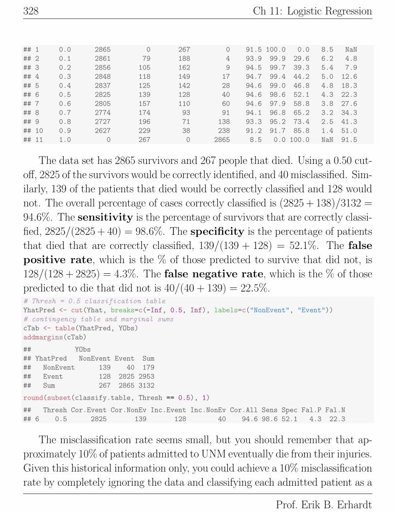
328 Ch 11: Logistic Regression
## 1 0.0 2865 0 267 0 91.5 100.0 0.0 8.5 NaN
## 2 0.1 2861 79 188 4 93.9 99.9 29.6 6.2 4.8
## 3 0.2 2856 105 162 9 94.5 99.7 39.3 5.4 7.9
## 4 0.3 2848 118 149 17 94.7 99.4 44.2 5.0 12.6
## 5 0.4 2837 125 142 28 94.6 99.0 46.8 4.8 18.3
## 6 0.5 2825 139 128 40 94.6 98.6 52.1 4.3 22.3
## 7 0.6 2805 157 110 60 94.6 97.9 58.8 3.8 27.6
## 8 0.7 2774 174 93 91 94.1 96.8 65.2 3.2 34.3
## 9 0.8 2727 196 71 138 93.3 95.2 73.4 2.5 41.3
## 10 0.9 2627 229 38 238 91.2 91.7 85.8 1.4 51.0
## 11 1.0 0 267 0 2865 8.5 0.0 100.0 NaN 91.5
The data set has 2865 survivors and 267 people that died. Using a 0.50 cut-
off, 2825 of the survivors would be correctly identified, and 40 misclassified. Sim-
ilarly, 139 of the patients that died would be correctly classified and 128 would
not. The overall percentage of cases correctly classified is (2825 + 138)/3132 =
94.6%. The sensitivity is the percentage of survivors that are correctly classi-
fied, 2825/(2825 + 40) = 98.6%. The specificity is the percentage of patients
that died that are correctly classified, 139/(139 + 128) = 52.1%. The false
positive rate, which is the % of those predicted to survive that did not, is
128/(128 + 2825) = 4.3%. The false negative rate, which is the % of those
predicted to die that did not is 40/(40 + 139) = 22.5%.# Thresh = 0.5 classification table
YhatPred <- cut(Yhat, breaks=c(-Inf, 0.5, Inf), labels=c("NonEvent", "Event"))
# contingency table and marginal sums
cTab <- table(YhatPred, YObs)
addmargins(cTab)
## YObs
## YhatPred NonEvent Event Sum
## NonEvent 139 40 179
## Event 128 2825 2953
## Sum 267 2865 3132
round(subset(classify.table, Thresh == 0.5), 1)
## Thresh Cor.Event Cor.NonEv Inc.Event Inc.NonEv Cor.All Sens Spec Fal.P Fal.N
## 6 0.5 2825 139 128 40 94.6 98.6 52.1 4.3 22.3
The misclassification rate seems small, but you should remember that ap-
proximately 10% of patients admitted to UNM eventually die from their injuries.
Given this historical information only, you could achieve a 10% misclassification
rate by completely ignoring the data and classifying each admitted patient as a
Prof. Erik B. Erhardt
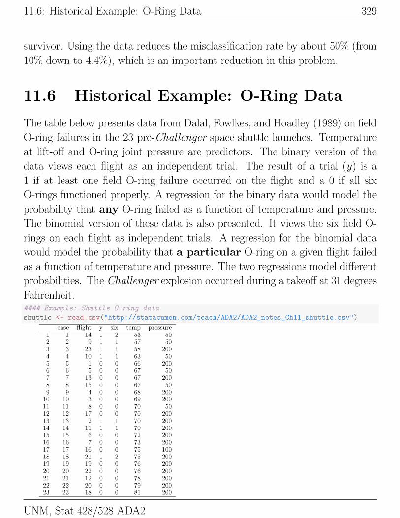
11.6: Historical Example: O-Ring Data 329
survivor. Using the data reduces the misclassification rate by about 50% (from
10% down to 4.4%), which is an important reduction in this problem.
11.6 Historical Example: O-Ring Data
The table below presents data from Dalal, Fowlkes, and Hoadley (1989) on field
O-ring failures in the 23 pre-Challenger space shuttle launches. Temperature
at lift-off and O-ring joint pressure are predictors. The binary version of the
data views each flight as an independent trial. The result of a trial (y) is a
1 if at least one field O-ring failure occurred on the flight and a 0 if all six
O-rings functioned properly. A regression for the binary data would model the
probability that any O-ring failed as a function of temperature and pressure.
The binomial version of these data is also presented. It views the six field O-
rings on each flight as independent trials. A regression for the binomial data
would model the probability that a particular O-ring on a given flight failed
as a function of temperature and pressure. The two regressions model different
probabilities. The Challenger explosion occurred during a takeoff at 31 degrees
Fahrenheit.#### Example: Shuttle O-ring data
shuttle <- read.csv("http://statacumen.com/teach/ADA2/ADA2_notes_Ch11_shuttle.csv")
case flight y six temp pressure1 1 14 1 2 53 502 2 9 1 1 57 503 3 23 1 1 58 2004 4 10 1 1 63 505 5 1 0 0 66 2006 6 5 0 0 67 507 7 13 0 0 67 2008 8 15 0 0 67 509 9 4 0 0 68 200
10 10 3 0 0 69 20011 11 8 0 0 70 5012 12 17 0 0 70 20013 13 2 1 1 70 20014 14 11 1 1 70 20015 15 6 0 0 72 20016 16 7 0 0 73 20017 17 16 0 0 75 10018 18 21 1 2 75 20019 19 19 0 0 76 20020 20 22 0 0 76 20021 21 12 0 0 78 20022 22 20 0 0 79 20023 23 18 0 0 81 200
UNM, Stat 428/528 ADA2

330 Ch 11: Logistic Regression
The regression model for the binomial data (i.e., six trials per launch) is
suspect on substantive grounds. The binomial model makes no allowance for
an effect due to having the six O-rings on the same flight. If these data were
measurements rather than counts, they would almost certainly be treated as
dependent repeated measures. If interest is focused on whether one or more
O-rings failed, the simplest, most direct data are the binary data.
Consider fitting a logistic regression model using temperature and pressure
as predictors. Let pi be the probability that any O-ring fails in case i and model
this as
log
(pi
1− pi
)= β0 + β1 Tempi + β2 Pressurei.
Logistic histogram plots of the data show a clear marginal relationship offailure with temp but not with pressure. We still need to assess the model withboth variables together.# plot logistic plots of response to each predictor individually
library(popbio)
logi.hist.plot(shuttle$temp, shuttle$y, boxp=FALSE, type="hist"
, rug=TRUE, col="gray", ylabel = "Probability", xlabel = "Temp")
logi.hist.plot(shuttle$pressure, shuttle$y, boxp=FALSE, type="hist"
, rug=TRUE, col="gray", ylabel = "Probability", xlabel = "Pressure")
55 60 65 70 75 80
0.0
0.2
0.4
0.6
0.8
1.0
Temp
Pro
babi
lity
0
5
10
10
5
0
Fre
quen
cy
0.0
0.2
0.4
0.6
0.8
1.0 ● ● ● ●
● ●●● ● ● ●●
●●
● ● ●
●
●● ● ● ●
50 100 150 200
0.0
0.2
0.4
0.6
0.8
1.0
Pressure
Pro
babi
lity
0
10
20
20
10
0
Fre
quen
cy
0.0
0.2
0.4
0.6
0.8
1.0 ●● ●●
●● ●● ●●● ●
●●
●●●
●
●●●●●
We fit the logistic model below using Y = 1 if at least one O-ring failed,
and 0 otherwise. We are modelling the chance of one or more O-ring failures
as a function of temperature and pressure.
The D goodness-of-fit statistic suggest no gross deviations from the model.
Prof. Erik B. Erhardt

11.6: Historical Example: O-Ring Data 331
Furthermore, the test of H0 : β1 = β2 = 0 (no regression effects) based on
the Wald test has a p-value of 0.1, which suggests that neither temperature or
pressure, or both, are useful predictors of the probability of O-ring failure. The
z-test test p-values for testing H0 : β1 = 0 and H0 : β2 = 0 individually are
0.037 and 0.576, respectively, which indicates pressure is not important (when
added last to the model), but that temperature is important. This conclusion
might be anticipated by looking at data plots above.glm.sh <- glm(cbind(y, 1 - y) ~ temp + pressure, family = binomial, shuttle)
# Test residual deviance for lack-of-fit (if > 0.10, little-to-no lack-of-fit)
dev.p.val <- 1 - pchisq(glm.sh$deviance, glm.sh$df.residual)
dev.p.val
## [1] 0.4589415
# Testing Global Null Hypothesis
library(aod)
coef(glm.sh)
## (Intercept) temp pressure
## 16.385319489 -0.263404073 0.005177602
# specify which coefficients to test = 0 (Terms = 2:3 is for terms 2 and 3)
wald.test(b = coef(glm.sh), Sigma = vcov(glm.sh), Terms = 2:3)
## Wald test:
## ----------
##
## Chi-squared test:
## X2 = 4.6, df = 2, P(> X2) = 0.1
# Model summary
summary(glm.sh)
##
## Call:
## glm(formula = cbind(y, 1 - y) ~ temp + pressure, family = binomial,
## data = shuttle)
##
## Deviance Residuals:
## Min 1Q Median 3Q Max
## -1.1928 -0.7879 -0.3789 0.4172 2.2031
##
## Coefficients:
## Estimate Std. Error z value Pr(>|z|)
## (Intercept) 16.385319 8.027474 2.041 0.0412 *
## temp -0.263404 0.126371 -2.084 0.0371 *
## pressure 0.005178 0.009257 0.559 0.5760
## ---
## Signif. codes: 0 '***' 0.001 '**' 0.01 '*' 0.05 '.' 0.1 ' ' 1
##
UNM, Stat 428/528 ADA2
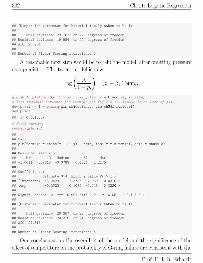
332 Ch 11: Logistic Regression
## (Dispersion parameter for binomial family taken to be 1)
##
## Null deviance: 28.267 on 22 degrees of freedom
## Residual deviance: 19.984 on 20 degrees of freedom
## AIC: 25.984
##
## Number of Fisher Scoring iterations: 5
A reasonable next step would be to refit the model, after omitting pressure
as a predictor. The target model is now
log
(pi
1− pi
)= β0 + β1 Tempi.
glm.sh <- glm(cbind(y, 1 - y) ~ temp, family = binomial, shuttle)
# Test residual deviance for lack-of-fit (if > 0.10, little-to-no lack-of-fit)
dev.p.val <- 1 - pchisq(glm.sh$deviance, glm.sh$df.residual)
dev.p.val
## [1] 0.5013827
# Model summary
summary(glm.sh)
##
## Call:
## glm(formula = cbind(y, 1 - y) ~ temp, family = binomial, data = shuttle)
##
## Deviance Residuals:
## Min 1Q Median 3Q Max
## -1.0611 -0.7613 -0.3783 0.4524 2.2175
##
## Coefficients:
## Estimate Std. Error z value Pr(>|z|)
## (Intercept) 15.0429 7.3786 2.039 0.0415 *
## temp -0.2322 0.1082 -2.145 0.0320 *
## ---
## Signif. codes: 0 '***' 0.001 '**' 0.01 '*' 0.05 '.' 0.1 ' ' 1
##
## (Dispersion parameter for binomial family taken to be 1)
##
## Null deviance: 28.267 on 22 degrees of freedom
## Residual deviance: 20.315 on 21 degrees of freedom
## AIC: 24.315
##
## Number of Fisher Scoring iterations: 5
Our conclusions on the overall fit of the model and the significance of the
effect of temperature on the probability of O-ring failure are consistent with the
Prof. Erik B. Erhardt

11.6: Historical Example: O-Ring Data 333
results for two predictor model. The model estimates the log-odds of (at least
one) O-ring failure to be
log
(p̃
1− p̃
)= 15.043− 0.2322 Temp.
The estimated probability of (at least one) O-ring failure is
p̃ =exp(15.043− 0.2322 Temp)
1 + exp(15.043− 0.2322 Temp).
This is an decreasing function of temperature.
The Challenger was set to launch on a morning where the predicted tem-
perature at lift-off was 31 degrees. Given that temperature appears to affect
the probability of O-ring failure (a point that NASA missed), what can/should
we say about the potential for O-ring failure?
Clearly, the launch temperature is outside the region for which data were
available. Thus, we really have no prior information about what is likely to
occur. If we assume the logistic model holds, and we can extrapolate back to
31 degrees, what is the estimated probability of O-ring failure?
The following gives the answer this question. I augmented the original data
set to obtain predicted probabilities for temperatures not observed in the data
set. Note that the fitted model to data with missing observations gives the same
model fit because glm() excludes observations with missing values. Predictions
are then made for all temperatures in the dataset and the resulting table and
plot are reported.# append values to dataset for which we wish to make predictions
shuttle.pred <- data.frame( case = rep(NA, 5)
, flight = rep(NA, 5)
, y = rep(NA, 5)
, six = rep(NA, 5)
, temp = c(31, 35, 40, 45, 50) # temp values to predict
, pressure = rep(NA, 5)
)
shuttle <- rbind(shuttle.pred, shuttle)
# fit model
glm.sh <- glm(cbind(y, 1 - y) ~ temp, family = binomial, shuttle)
# Note: same model fit as before since glm() does not use missing values
UNM, Stat 428/528 ADA2

334 Ch 11: Logistic Regression
round(summary(glm.sh)$coefficients, 3)
## Estimate Std. Error z value Pr(>|z|)
## (Intercept) 15.043 7.379 2.039 0.041
## temp -0.232 0.108 -2.145 0.032
# put the fitted values in the data.frame
shuttle$fitted.values <- c(rep(NA, 5), glm.sh$fitted.values)
# predict() uses all the temp values in dataset, including appended values
pred <- predict(glm.sh, data.frame(temp = shuttle$temp), type = "link", se.fit = TRUE)
shuttle$fit <- pred$fit
shuttle$se.fit <- pred$se.fit
# CI for fitted values
shuttle <- within(shuttle, {# added "fitted" to make predictions at appended temp values
fitted = exp(fit) / (1 + exp(fit))
fit.lower = exp(fit - 1.96 * se.fit) / (1 + exp(fit - 1.96 * se.fit))
fit.upper = exp(fit + 1.96 * se.fit) / (1 + exp(fit + 1.96 * se.fit))
})
case flight y six temp pressure fitted.values fit se.fit fit.upper fit.lower fitted1 31.00 7.85 4.04 1.00 0.48 1.002 35.00 6.92 3.61 1.00 0.46 1.003 40.00 5.76 3.08 1.00 0.43 1.004 45.00 4.60 2.55 1.00 0.40 0.995 50.00 3.43 2.02 1.00 0.37 0.976 1.00 14.00 1.00 2.00 53.00 50.00 0.94 2.74 1.71 1.00 0.35 0.947 2.00 9.00 1.00 1.00 57.00 50.00 0.86 1.81 1.31 0.99 0.32 0.868 3.00 23.00 1.00 1.00 58.00 200.00 0.83 1.58 1.21 0.98 0.31 0.839 4.00 10.00 1.00 1.00 63.00 50.00 0.60 0.42 0.77 0.87 0.25 0.60
10 5.00 1.00 0.00 0.00 66.00 200.00 0.43 −0.28 0.59 0.71 0.19 0.4311 6.00 5.00 0.00 0.00 67.00 50.00 0.38 −0.51 0.56 0.64 0.17 0.3812 7.00 13.00 0.00 0.00 67.00 200.00 0.38 −0.51 0.56 0.64 0.17 0.3813 8.00 15.00 0.00 0.00 67.00 50.00 0.38 −0.51 0.56 0.64 0.17 0.3814 9.00 4.00 0.00 0.00 68.00 200.00 0.32 −0.74 0.55 0.58 0.14 0.3215 10.00 3.00 0.00 0.00 69.00 200.00 0.27 −0.98 0.56 0.53 0.11 0.2716 11.00 8.00 0.00 0.00 70.00 50.00 0.23 −1.21 0.59 0.49 0.09 0.2317 12.00 17.00 0.00 0.00 70.00 200.00 0.23 −1.21 0.59 0.49 0.09 0.2318 13.00 2.00 1.00 1.00 70.00 200.00 0.23 −1.21 0.59 0.49 0.09 0.2319 14.00 11.00 1.00 1.00 70.00 200.00 0.23 −1.21 0.59 0.49 0.09 0.2320 15.00 6.00 0.00 0.00 72.00 200.00 0.16 −1.67 0.70 0.43 0.05 0.1621 16.00 7.00 0.00 0.00 73.00 200.00 0.13 −1.90 0.78 0.40 0.03 0.1322 17.00 16.00 0.00 0.00 75.00 100.00 0.09 −2.37 0.94 0.37 0.01 0.0923 18.00 21.00 1.00 2.00 75.00 200.00 0.09 −2.37 0.94 0.37 0.01 0.0924 19.00 19.00 0.00 0.00 76.00 200.00 0.07 −2.60 1.03 0.36 0.01 0.0725 20.00 22.00 0.00 0.00 76.00 200.00 0.07 −2.60 1.03 0.36 0.01 0.0726 21.00 12.00 0.00 0.00 78.00 200.00 0.04 −3.07 1.22 0.34 0.00 0.0427 22.00 20.00 0.00 0.00 79.00 200.00 0.04 −3.30 1.32 0.33 0.00 0.0428 23.00 18.00 0.00 0.00 81.00 200.00 0.02 −3.76 1.51 0.31 0.00 0.02
library(ggplot2)
p <- ggplot(shuttle, aes(x = temp, y = y))
# predicted curve and point-wise 95% CI
p <- p + geom_ribbon(aes(x = temp, ymin = fit.lower, ymax = fit.upper), alpha = 0.2)
p <- p + geom_line(aes(x = temp, y = fitted), colour="red")
# fitted values
Prof. Erik B. Erhardt
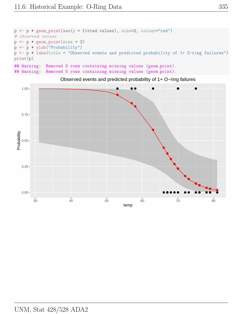
11.6: Historical Example: O-Ring Data 335
p <- p + geom_point(aes(y = fitted.values), size=2, colour="red")
# observed values
p <- p + geom_point(size = 2)
p <- p + ylab("Probability")
p <- p + labs(title = "Observed events and predicted probability of 1+ O-ring failures")
print(p)
## Warning: Removed 5 rows containing missing values (geom point).
## Warning: Removed 5 rows containing missing values (geom point).
●
●
●
●
●
●●●
●
●
●●●●
●●
●●●●
● ●●
● ● ● ●
● ●●● ● ● ●●
●●
● ● ●
●
●● ● ● ●0.00
0.25
0.50
0.75
1.00
30 40 50 60 70 80temp
Pro
babi
lity
Observed events and predicted probability of 1+ O−ring failures
UNM, Stat 428/528 ADA2