1 

 

Predicting Charitable Contributions

By Lauren Meyer

Executive Summary Charitable contributions depend on many factors from financial security to personal characteristics. This report will focus on demographic and financial information from 2000 families who participated in the 2004 Survey of Consumer Finance. Specifically, two regression models are introduced. The first serves to indicate whether or not a family will make any charitable contribution, while the second serves to predict the amount of the contribution. The models pinpoint certain financial and demographic information to be important determinants of charitable contributions. Among other things, both models find that older, more educated families with greater incomes, savings, and inheritances are likely to contribute more money to charity. Section 1. Introduction Charitable contributions are one thing that society values. As a society, we almost expect people making over some threshold to contribute large amounts to charity. Many ask: “why does one person need all that wealth?” Even your average citizen usually enjoys contributing to a cause in which they believe. Yet people’s behaviors tend to vary a great deal, even in similar situations. Despite this, is it possible to accurately predict charitable contributions of individuals and families? It is logical to think that one’s personal values will influence the amount they contribute to charity. There are some very generous people who find ways to donate even when they themselves are not in the best financial position. Personal characteristics, such as generosity, selflessness, and the degree to which one is materialistic, could all be influential in predicting charitable contributions. However, there must be some more objective financial evidence that can serve as a better predictor of charitable contributions. Personal characteristics aside, we would expect a billionaire to contribute more to charity than someone with an income of $30,000 per year. Income, along with numerous other financial measures, could be considered important predictors of charitable contributions. This report serves to use data from the 2004 Survey of Consumer Finance (SCF) in order to estimate charitable contributions of families, given that we know some demographic and financial information about them. The SCF is conducted by the Federal Reserve Board and collects information concerning the balance sheet, pension, income, and other demographic characteristics of U.S. families. One question asked of these U.S. families is the amount of their charitable contributions in 2003, which will be the key variable of interest for this report.

The remainder of the report will be organized as follows. Section 2 will explain important characteristics of the data. Section 3 will explore the model chosen to represent the data in hopes of explaining charitable contributions as best as possible. Section 4 will have concluding thoughts. Finally, more detailed analysis is provided in the appendices. Section 2. Data Characteristics The SCF is a cross-sectional survey that is nationally representative. Observational data is collected every three years by the National Opinion Research Center, a national organization for research and computing at the University of Chicago, via on-site and phone interviews. In order to study the factors affecting charitable contributions, two thousand observations were randomly selected from the SCF database. Two thousand observations are enough to ensure a representative sample, yet are easier to work with than the original forty-five hundred observations. When examining charitable contributions, it is expected that many families will not contribute anything to charity. On the other hand, for those who do contribute to charity, there are a wide range of amounts contributed. Based on this understanding, I found it best to first predict whether or not the family made a charitable contribution using all two thousand data points. Next, I would predict how much a given charitable contribution would be, using only observations with positive charitable contributions. Out of the two thousand observations from the SCF, one thousand fifty households contributed something to charity. The smallest contribution amount reported was five hundred dollars, while the largest amount contributed to charity was $9,070,000. Figure 1 below shows the distribution of charitable contributions, after removing the observations with no contribution. The numbers above the bars indicate how many observations fell into that range.

Figure 1.

2 

 

From Figure 1, notice that 1032 of the 1050 observations, or more than 98% of positive charitable contributions, were for amounts of $1000 or less. This graph indicates that the data is skewed to the right. A logarithmic transformation will be used for charitable contributions in order to symmetrize this skewed distribution. This transformation is useful, as it will pull-in extreme contribution values, yet will retain the original ordering, such that the largest contribution amounts are still the largest amounts on the logarithmic scale. Figure 2 shows the new distribution of charitable contributions, after performing a logarithmic transformation. While this transformation does not perfectly symmetrize the data, it does serve well in spreading out the observations.

Figure 2.

Distribution of Logarithmic Charitable Contributions

Logarithmic Charitable Contribution

6 8 10 12 14 16

0

50

100

150

200

250

300304

190

210

125

97

5237

218 4 2

Up to this point, I have not yet introduced the variables that will be used to predict charitable contributions. The SCF has more than 5,000 questions that were answered by participating families. Of these variables, there are many which could impact charitable contributions. The details of variable selection for this report will be discussed more in section three.

3 

 

There are, of course, some variables that we expect to have a great influence on charitable contributions. For example, it seems reasonable that income would be a strong predictor of charitable contributions. Figure 3 identifies the relationship between income and logarithmic charitable contributions, which was decided upon as the dependent variable of

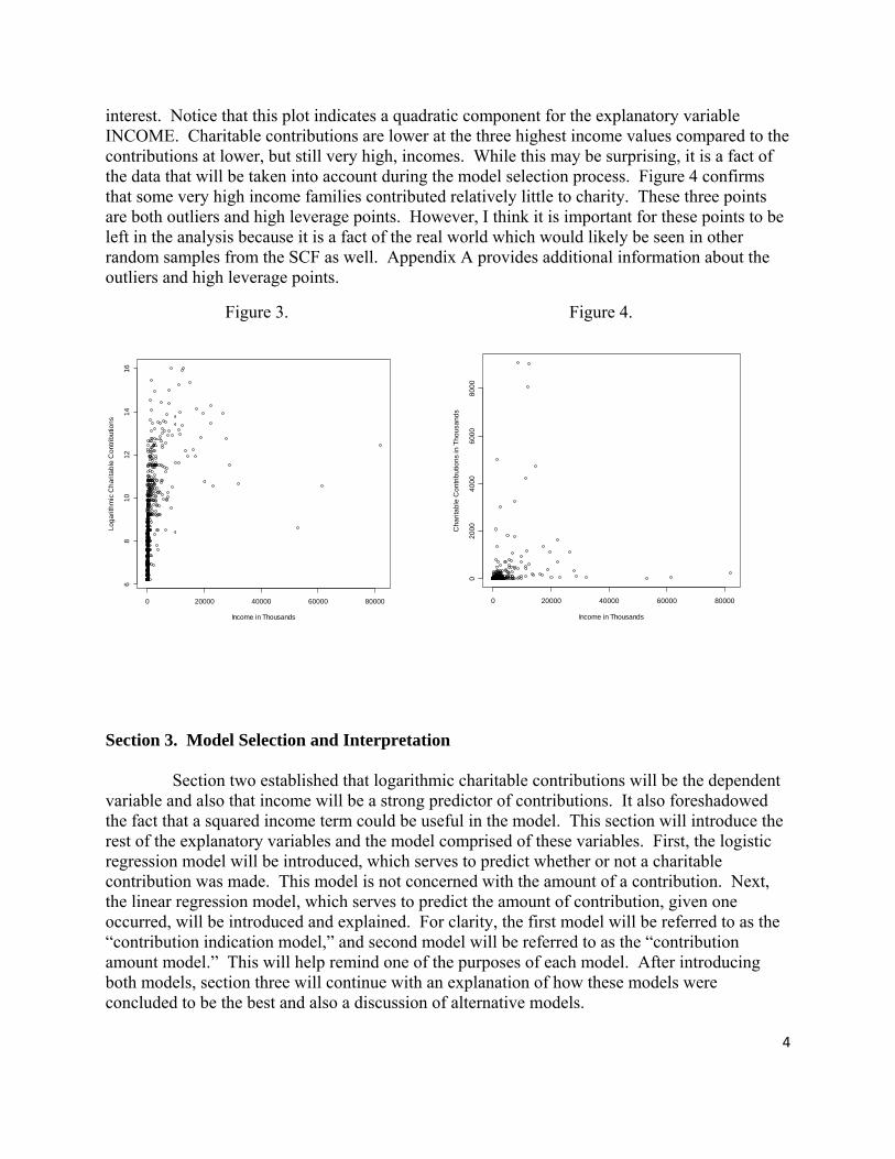
interest. Notice that this plot indicates a quadratic component for the explanatory variable INCOME. Charitable contributions are lower at the three highest income values compared to the contributions at lower, but still very high, incomes. While this may be surprising, it is a fact of the data that will be taken into account during the model selection process. Figure 4 confirms that some very high income families contributed relatively little to charity. These three points are both outliers and high leverage points. However, I think it is important for these points to be left in the analysis because it is a fact of the real world which would likely be seen in other random samples from the SCF as well. Appendix A provides additional information about the outliers and high leverage points.

Figure 3. Figure 4.

0 20000 40000 60000 80000

68

1012

1416

Income in Thousands

Loga

rithm

ic C

harit

able

Con

tribu

tions

0 20000 40000 60000 80000

020

0040

0060

0080

00

Income in Thousands

Cha

ritab

le C

ontri

butio

ns in

Tho

usan

ds

Section 3. Model Selection and Interpretation Section two established that logarithmic charitable contributions will be the dependent variable and also that income will be a strong predictor of contributions. It also foreshadowed the fact that a squared income term could be useful in the model. This section will introduce the rest of the explanatory variables and the model comprised of these variables. First, the logistic regression model will be introduced, which serves to predict whether or not a charitable contribution was made. This model is not concerned with the amount of a contribution. Next, the linear regression model, which serves to predict the amount of contribution, given one occurred, will be introduced and explained. For clarity, the first model will be referred to as the “contribution indication model,” and second model will be referred to as the “contribution amount model.” This will help remind one of the purposes of each model. After introducing both models, section three will continue with an explanation of how these models were concluded to be the best and also a discussion of alternative models.

4 

 

5 

 

Contribution Indication Model The contribution indication model is a nonlinear, logistic regression model with the following dependent variables and regression coefficients:

Explanatory Variables  Coefficient   Z‐Value   

   ‐1.990 ‐8.514 *** Income  1.327E‐06 3.161 ** Age  1.537E‐02 3.472 *** Pension, Annuities Income  1.005E‐05 2.092 * Life Insurance (FACE AMT)  7.622E‐07 3.407 *** Spouse Age  1.054E‐02 4.353 *** # Businesses Managed  4.700E‐01 3.904 *** Savings Bond Value  6.252E‐05 2.824 ** Support to Family/Friends  2.485E‐05 2.131 * Spouse Education (=Bachelors)  6.145E‐01 4.681 *** Spouse Education (=Masters)  1.355E+00 5.585 *** Amount Owed on Mortgages  3.136E‐06 4.857 *** Total Savings  1.939E‐06 1.937 . Total Inherited  4.717E‐07 1.352   Assets  ‐7.811E‐08 ‐2.467 * Saving Habits (Not regularly)  ‐5.326E‐01 ‐4.554 *** 

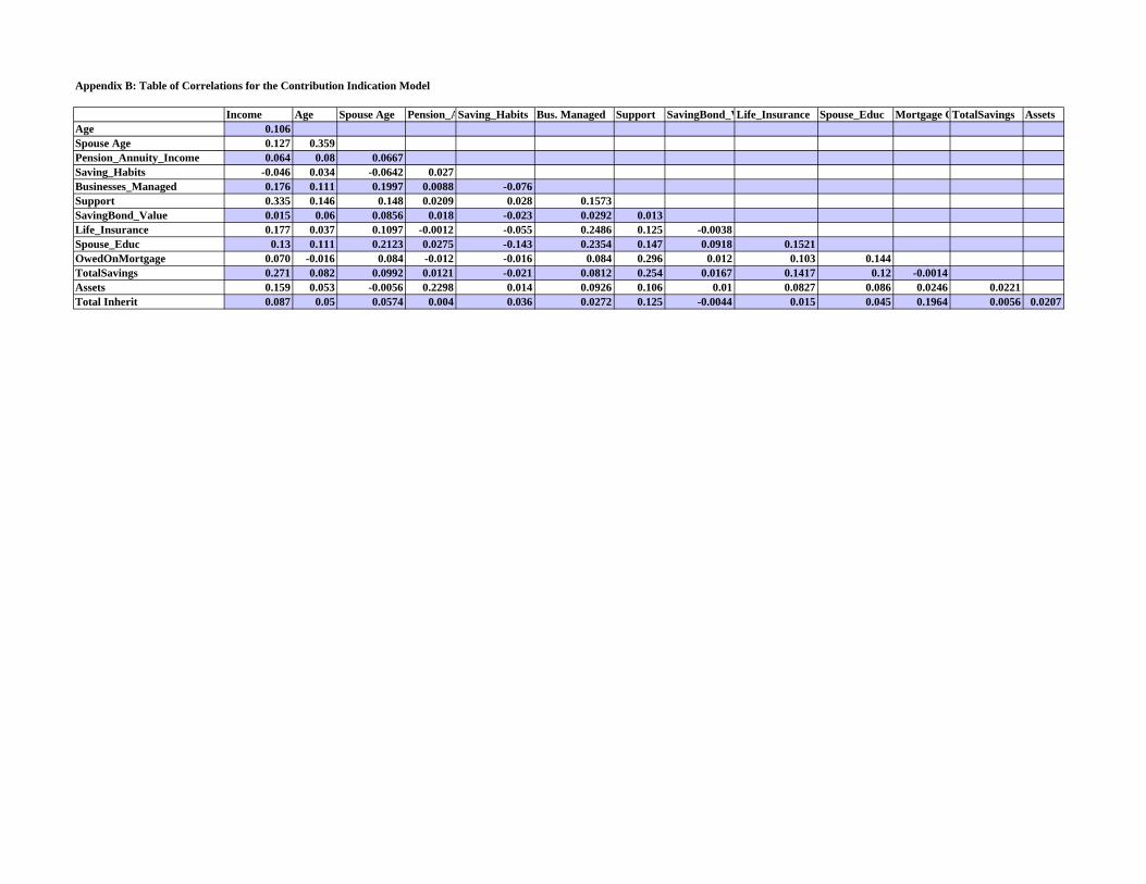
The coefficients in the above table provide information about how the explanatory variables will affect the dependent variable, which is a binary variable with a value of 1 if a charitable contribution occurred. For instance, the negative coefficient associated with saving habits indicates that a family who does not save regularly will be less likely to make a charitable contribution. The z-values are another important statistics associated with each variable. The larger the z-value, the more significant that variable is in explaining charitable contributions. The asterisks also serve as a significance indicator. For example, the *** indicates that the variable is significant at the one-tenth of a percent level. Many of the variables and coefficients in this model seem reasonable, maybe even expected. It makes sense that a family with more income would be more likely to make a charitable contribution. Other variables such as AGE and SPOUSE AGE have a positive coefficient indicating that older families are more likely to contribute to charity. This could be true because older households do not need to support children anymore. LIFE INSURANCE amount and number of BUSINESSES_MANAGED are also positively related to charitable contributions. This is partly because they are positively correlated with income. Appendix B contains a table of correlation coefficients for the contribution indication model. Also, business managers may be more likely to contribute to charity because it creates a good image for their company.

6 

 

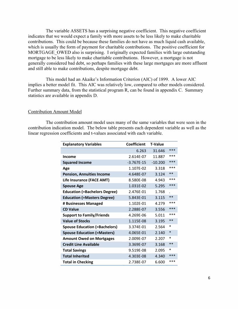
The variable ASSETS has a surprising negative coefficient. This negative coefficient indicates that we would expect a family with more assets to be less likely to make charitable contributions. This could be because these families do not have as much liquid cash available, which is usually the form of payment for charitable contributions. The positive coefficient for MORTGAGE_OWED also is surprising. I originally expected families with large outstanding mortgage to be less likely to make charitable contributions. However, a mortgage is not generally considered bad debt, so perhaps families with these large mortgages are more affluent and still able to make contributions, despite mortgage debt. This model had an Akaike’s Information Criterion (AIC) of 1899. A lower AIC implies a better model fit. This AIC was relatively low, compared to other models considered. Further summary data, from the statistical program R, can be found in appendix C. Summary statistics are available in appendix D. Contribution Amount Model The contribution amount model uses many of the same variables that were seen in the contribution indication model. The below table presents each dependent variable as well as the linear regression coefficients and t-values associated with each variable.

Explanatory Variables  Coefficient  T‐Value    

   6.263  31.646 *** Income  2.614E‐07  11.887 *** Squared Income  ‐3.767E‐15  ‐10.200 *** Age  1.107E‐02  3.318 *** Pension, Annuities Income  4.648E‐07  3.124 ** Life Insurance (FACE AMT)  8.580E‐08  4.943 *** Spouse Age  1.031E‐02  5.295 *** Education (=Bachelors Degree)  2.476E‐01  1.768 . Education (=Masters Degree)  5.843E‐01  3.115 ** # Businesses Managed  1.102E‐01  4.279 *** CD Value  2.288E‐07  3.556 *** Support to Family/Friends  4.269E‐06  5.011 *** Value of Stocks  1.115E‐08  3.195 ** Spouse Education (=Bachelors)  3.374E‐01  2.564 * Spouse Education (=Masters)  4.065E‐01  2.140 * Amount Owed on Mortgages  2.009E‐07  2.207 * Credit Line Available  3.369E‐07  3.168 ** Total Savings  9.519E‐08  2.095 * Total Inherited  4.303E‐08  4.340 *** Total in Checking  2.738E‐07  6.600 *** 

7 

 

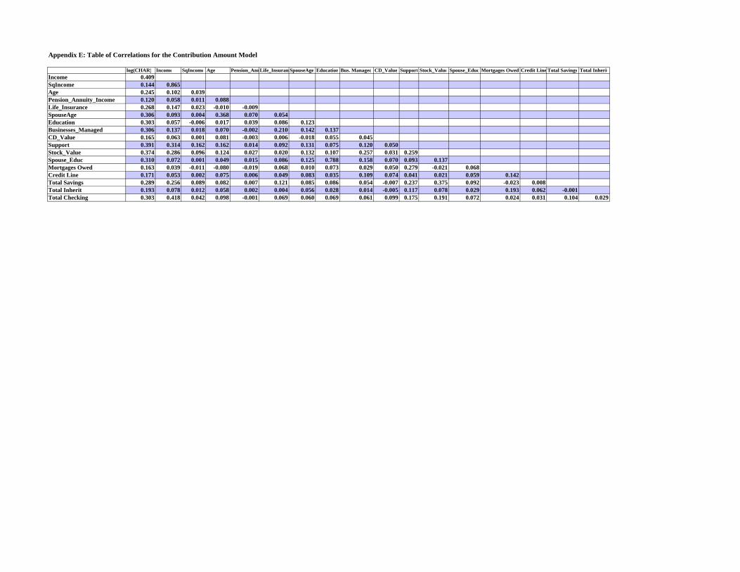
One important variable in the model is SQUARED INCOME. This variable was added based on the plot of LOG(CHARITABLE_CONT) vs. INCOME that was shown in section two. SQUARED INCOME has a negative coefficient, as expected, indicating that as INCOME is increasing, LOG(CHARITABLE_CONT) is increasing at a decreasing rate. This squared term also explains the decreasing contribution amounts at very large income levels. Interestingly, CD_VALUE and STOCK_VALUE were useful in predicting a contribution amount, rather than BOND_VALUE, which was important in the contribution indication model. Both CD and stock value have positive coefficients indicating higher amounts in CDs and stocks is generally associated with a larger charitable contribution. In this model, EDUCATION of the respondent was now an important explanatory variable in addition to SPOUSE _EDUCATION, which was seen in the contribution indication model. Higher education levels are generally associated with high income levels, although the correlation coefficients between education and income for this data set were not strong. Appendix E has correlation coefficients for the contribution amount model. T-values, like z-values, indicate how significant each variable is in predicting LOG(CHARITABLE_CONT). Every variable except EDUCATION (=BACHELORS) has a t-value greater than two in absolute value. The coefficient of determination for this model, R2 = .554, indicates that the model explains 55.4% of the variability in charitable contributions. The coefficient of determination adjusted for degrees of freedom, Ra

2 = .5458, was not much lower. The size of the typical error, s, was 1.33. Further summary data from the statistical program R can be found in appendix F. Summary statistics for this model are in appendix G. One concern with this model was related to the presence of collinearity, which occurs when one explanatory variable is nearly a linear combination of the other explanatory variables. To examine the presence of collinearity, variance inflation factors (VIF) were calculated for each variable. The highest VIF was that of INCOME with a value of 6.14. While this is somewhat large, it is not greater than 10, at which point severe collinearity would exist. The VIF for the other variables can be found in appendix H.

8 

 

An Example using these Models An example will help clarify how to use the two aforementioned models. Suppose we have the following information about the Smith family:

• Mr. Smith was the survey respondent. • Family income is $140,000 per year. • The family is receiving no pension or annuity income. • The family holds a life insurance policy on Mr. Smith with FACE amount of $500,000. • Mr. Smith is 46 and Mrs. Smith is 42. • Both Mr. and Mrs. Smith have earned bachelor’s degrees. • They do not manage any businesses and do not support family or friends, monetarily. • They have CDs worth $15,000, Stocks worth $20,000, and Savings Bonds for $10,000. • They still owe $100,000 on their mortgage. • They own a yacht worth $40,000 – which is considered ASSETS. • Their available credit line is $50,000. • The Smiths have $50,000 in savings and $25,000 in checking. • They recently inherited $100,000 when Mr. Smith’s father passed away. • Their savings habits are defined as regular by the SCF.

First, using the contribution indication model, we can find the probability that the Smiths

make a charitable contribution. Π(z) will be used to denote the logit regression case.

Π(z) = -1.990 + (1.327E-06)(140,000) + (1.537E-02 )(46) + (7.622E-07)(500,000) + (1.054E-02)(42) + (6.252E-05)(10,000) + 6.145E-01 + (3.136E-06)(100,000) + (1.939E-06)(50,000) + (4.717E-07)(100,000) + (-7.811E-08)(40,000) = 1.42071

For the logit case, Π(z) = ez/(1+ez) or in this case e(1.42071)/(1+e(1.42071)). The probability that the Smiths make some contribution to charity is .805.

Next let’s see how much we would expect the Smiths to contribute to charity, given they make a contribution.

Log(Contribution) = 6.263 + (2.614E-07)(140,000) + (-3.767E-15)(140,000^2) + (1.107E-02)(46) + (8.580E-08)(500,000) + (1.031E-02)(42) + (2.476E-01) + (2.288E-07)(15,000) + (1.115E-08)(20,000) + 3.374E-01 + (2.009E-07)(100,000) + (3.369E-07)(50,000) + (9.519E-08)(50,000) + (4.303E-08)(100,000) + (2.738E-07)(25,000) = 7.925521

Since log(Contributions) = 7.92, we expect the Smiths to contribute $2,767 to charity.

9 

 

Determining the Final Models Both models are fairly complex due to the large number of variables. However, this was expected, as charitable contributions are a complex prediction to make. Many other models were considered, but the two chosen models provide the best estimates. Goodness of fit measures were already discussed in section two. Stepwise regression was used as a first step in determining both models. This was important to use because the original data set had over five thousand variables. After narrowing these down to 70 variables, which can been seen in appendix I, stepwise regression was run for the logistic and linear regression models. The final model is not exactly what was recommended from the stepwise regression. After looking at scatter plots, correlations, and variable coefficients, the final model was created. As section two demonstrated, the scatter plot of log(CHARITABLE CONT) vs. INCOME indicated the squared income term, which would not be identified by stepwise regression. In section two, it was also noted that three points were both outliers and high leverage points. After removing the three most unusual points, as identified in the residuals vs. leverages plot, the Ra

2 increased to 56.2% from 54.6%. Appendix J has more information about the regression model after removing these three points. These points were left in the data during model selection. One drawback of the contribution amount model is evident after looking at the residuals vs. fitted plot in appendix K. This plot indicates that heteroscedasticity is present. The variance of the residuals starts out relatively small, grows, and then slightly decreases. The plot also shows residuals becoming more consistently negative as fitted values increase. In other words, the model is overestimating charitable contributions for observations with large fitted values. Despite this, the chosen model is still the best, as all other models considered had this same problem. I feel more qualitative variables are necessary to solve this issue. This idea will be expanded upon in the recommendations portion of section four. Also relating to residuals, the histogram of standardized residuals appears normally distributed. Alternative Models One alternative model to be considered involves adding an INCOME^3 term. Doing this increases the Ra

2 to 59.7% and also improves the residual versus fitted plot discussed earlier. I did not use this term because it increases the model complexity. Also, I questioned whether an INCOME^3 term made economical sense and whether the term would be significant if a different data sample from the SCF was taken. As mentioned earlier, the data used for this report was a subset of 2000 from the 4500 observations in the SCF. I would suggest rerunning the contribution amount model introduced above with all 4500 observations. At this point, it would easier to consider whether INCOME^3 would actually be useful. The reason is that my subset of 2000 had only three data points with

10 

 

INCOME well over $40,000,000. These data points are influential in the analysis, and it would be useful to have more data points with such extremely high INCOME. Section 4. Summary and Concluding Remarks Despite the wide range of variability associated with charitable contributions, we know that it is possible to predict both whether a family will make a contribution and also how much that contribution would be. The recommended explanatory variables for indicating the probability that a contribution will be made are: the family’s income level, the age of the respondent and their spouse, amount of life insurance purchased, amount of income from pensions or annuities, number of businesses managed, amount of support provided to others, amount of money in bonds, savings, and assets, total amount inherited, spouse’s education level, amount owed on mortgages, and saving habits of the family. To predict the amount of money likely to be contributed to charity, the following additional variables are recommended: Income squared, education level of the respondent, value of CDs and stocks, the total amount in checking, and the credit line available to the family. The study looked at cross-sectional data from the Survey of Consumer Finance, which mainly has demographic and financial information about families. I believe the coefficient of determination, R2, could be dramatically improved if additional data sources could be brought into the study. Mainly, subjective information would improve the study, such as how important one feels it is to donate to charity and other personal attributes that reflect how caring, giving, and materialistic the respondent is. It would also be interesting to consider a more longitudinal study, by looking at how much charitable contributions change for the same families year after year. This would allow personal characteristics to be held steadier, and the focus could be turned to financial variables, as we would expect salary and net worth to be increasing with time.

11 

 

Appendices: Table of Contents

Appendix A: Standardized residuals vs. Leverages for the Contribution Amount Model Appendix B: Table of Correlations for the Contribution Indication Model Appendix C: Summary data for predicting whether a contribution was made Appendix D: Summary Statistics for the Contribution Indication Model Appendix E: Table of Correlations for the Contribution Amount Model Appendix F: Summary data for predicting the amount of a charitable contribution Appendix G: Summary Statistics for the Contribution Amount Model Appendix H: Variance Inflation Factors Appendix I: Variables Considered from the SCF and Variables Created from the SCF Appendix J: R output after removing three unusual points Appendix K: Residuals vs. Fitted Values for the Contribution Amount Model

Appendix A: Residuals vs. Leverage for the Contribution Amount Model

Observation Number Standardized Residual Leverage

1185 5.40 .773 1683 -4.22 .517 1956 -4.22 .389

Appendix B: Table of Correlations for the Contribution Indication Model

Income Age Spouse Age Pension_ASaving_Habits Bus. Managed Support SavingBond_VLife_Insurance Spouse_Educ Mortgage OTotalSavings AssetsAge 0.106Spouse Age 0.127 0.359Pension_Annuity_Income 0.064 0.08 0.0667Saving_Habits -0.046 0.034 -0.0642 0.027Businesses_Managed 0.176 0.111 0.1997 0.0088 -0.076Support 0.335 0.146 0.148 0.0209 0.028 0.1573SavingBond_Value 0.015 0.06 0.0856 0.018 -0.023 0.0292 0.013Life_Insurance 0.177 0.037 0.1097 -0.0012 -0.055 0.2486 0.125 -0.0038Spouse_Educ 0.13 0.111 0.2123 0.0275 -0.143 0.2354 0.147 0.0918 0.1521OwedOnMortgage 0.070 -0.016 0.084 -0.012 -0.016 0.084 0.296 0.012 0.103 0.144TotalSavings 0.271 0.082 0.0992 0.0121 -0.021 0.0812 0.254 0.0167 0.1417 0.12 -0.0014Assets 0.159 0.053 -0.0056 0.2298 0.014 0.0926 0.106 0.01 0.0827 0.086 0.0246 0.0221Total Inherit 0.087 0.05 0.0574 0.004 0.036 0.0272 0.125 -0.0044 0.015 0.045 0.1964 0.0056 0.0207

Appendix C. Summary Data for Model 1: Predicting whether a contribution was made Call: glm(formula = CharityInd ~ AGE + SPOUSEAGE + INCOME + Pension_Annuity_Income + factor(Saving_Habits) + Businesses_Managed + Support + SavingBond_Value + Life_Insurance + factor(Spouse_Educ) + OwedOnMortgages + TotalSavings + Assets + TotalInherit, family = binomial(link = logit), data = mydata) Deviance Residuals: Min 1Q Median 3Q Max -4.248e+00 -7.664e-01 6.672e-05 7.566e-01 2.131e+00 Coefficients: Estimate Std. Error z value Pr(>|z|) (Intercept) -1.990e+00 2.337e-01 -8.514 < 2e-16 *** AGE 1.537e-02 4.427e-03 3.472 0.000516 *** SPOUSEAGE 1.054e-02 2.422e-03 4.353 1.34e-05 *** INCOME 1.327e-06 4.198e-07 3.161 0.001574 ** Pension_Annuity_Income 1.005e-05 4.806e-06 2.092 0.036480 * factor(Saving_Habits)5 -5.326e-01 1.170e-01 -4.554 5.27e-06 *** Businesses_Managed 4.700e-01 1.204e-01 3.904 9.46e-05 *** Support 2.485e-05 1.166e-05 2.131 0.033081 * SavingBond_Value 6.252e-05 2.214e-05 2.824 0.004744 ** Life_Insurance 7.622e-07 2.237e-07 3.407 0.000657 *** factor(Spouse_Educ)2 6.145e-01 1.313e-01 4.681 2.85e-06 *** factor(Spouse_Educ)3 1.355e+00 2.427e-01 5.585 2.34e-08 *** OwedOnMortgages 3.136e-06 6.455e-07 4.857 1.19e-06 *** TotalSavings 1.939e-06 1.001e-06 1.937 0.052755 . Assets -7.811e-08 3.165e-08 -2.467 0.013608 * TotalInherit 4.717e-07 3.488e-07 1.352 0.176242 Null deviance: 2767.6 on 1999 degrees of freedom Residual deviance: 1867.6 on 1984 degrees of freedom AIC: 1899.6 Number of Fisher Scoring iterations: 9 Appendix D:  Summary Statistics for the Contribution Indication Model   Variable  Mean  Median  SD  Min  Max 

INCOME  701,000.00  54,000.00 3,440,000.00 ‐250,000.00 82,000,000.00 AGE  50.90  51.00  15.80  18.00  95.00 Pension_Annuity_Income  13,300.00  0.00  204,000.00  0.00  9,000,000.00 Life_Insurance  459,000.00  7,250.00  1,880,000.00 0.00  30,000,000.00 SPOUSEAGE  32.60  39.00  25.40  0.00  89.00 Businesses_Managed  0.48  0.00  1.34  0.00  25.00 Support  8,390.00  0.00  41,400.00  0.00  560,000.00 SavingBond_Value  2,120.00  0.00  17,700.00  0.00  40,000.00 OwedOnMortgages  106,000.00  50.00  753,000.00  0.00  20,000,000.00 Total Savings  100,000.00  50.00  753,000.00  0.00  20,000,000.00 Assets  251,000.00  0.00  4,070,000.00 ‐315,000.00 165,000,000.00 

TotalInherit  196,000.00  0.00  3,120,000.00 0.00  115,000,000.00 

Appendix E: Table of Correlations for the Contribution Amount Model

log(CHAR) Income SqIncome Age Pension_AnnLife_Insuran SpouseAge Education Bus. Managed CD_Value Support Stock_Value Spouse_Educ Mortgages Owed Credit Line Total Savings Total InheritIncome 0.409SqIncome 0.144 0.865Age 0.245 0.102 0.039Pension_Annuity_Income 0.120 0.058 0.011 0.088Life_Insurance 0.268 0.147 0.023 -0.010 -0.009SpouseAge 0.306 0.093 0.004 0.368 0.070 0.054Education 0.303 0.057 -0.006 0.017 0.039 0.086 0.123Businesses_Managed 0.306 0.137 0.018 0.070 -0.002 0.210 0.142 0.137CD_Value 0.165 0.063 0.001 0.081 -0.003 0.006 -0.018 0.055 0.045Support 0.391 0.314 0.162 0.162 0.014 0.092 0.131 0.075 0.120 0.050Stock_Value 0.374 0.286 0.096 0.124 0.027 0.020 0.132 0.107 0.257 0.031 0.259Spouse_Educ 0.310 0.072 0.001 0.049 0.015 0.086 0.125 0.788 0.158 0.070 0.093 0.137Mortgages Owed 0.163 0.039 -0.011 -0.080 -0.019 0.068 0.010 0.073 0.029 0.050 0.279 -0.021 0.068Credit Line 0.171 0.053 0.002 0.075 0.006 0.049 0.083 0.035 0.109 0.074 0.041 0.021 0.059 0.142Total Savings 0.289 0.256 0.089 0.082 0.007 0.121 0.085 0.086 0.054 -0.007 0.237 0.375 0.092 -0.023 0.008Total Inherit 0.193 0.078 0.012 0.058 0.002 0.004 0.056 0.028 0.014 -0.005 0.117 0.078 0.029 0.193 0.062 -0.001Total Checking 0.303 0.418 0.042 0.098 -0.001 0.069 0.060 0.069 0.061 0.099 0.175 0.191 0.072 0.024 0.031 0.104 0.029

Appendix F. Summary Data for Model 2: Predicting the amount of a charitable contribution Call: lm(formula = lnCHAR ~ INCOME + SqIncome + AGE + Pension_Annuity_Income + Life_Insurance + SPOUSEAGE + factor(EDUCATION) + Businesses_Managed + CD_Value + Support + Stock_Value + factor(Spouse_Educ) + OwedOnMortgages + CreditLine + TotalSavings + TotalInherit + TotalChecking, data = PositiveCont) Residuals: Min 1Q Median 3Q Max

-4.5196 -0.9091 -0.1534 0.8874 5.8488 Coefficients: Estimate Std. Error t value Pr(>|t|) (Intercept) 6.263e+00 1.979e-01 31.646 < 2e-16 *** INCOME 2.614e-07 2.199e-08 11.887 < 2e-16 *** SqIncome -3.767e-15 3.694e-16 -10.200 < 2e-16 *** AGE 1.107e-02 3.336e-03 3.318 0.000939 *** Pension_Annuity_Income 4.648e-07 1.488e-07 3.124 0.001835 ** Life_Insurance 8.580e-08 1.736e-08 4.943 9.00e-07 *** SPOUSEAGE 1.031e-02 1.947e-03 5.295 1.45e-07 *** factor(EDUCATION)2 2.476e-01 1.400e-01 1.768 0.077315 . factor(EDUCATION)3 5.843e-01 1.875e-01 3.115 0.001887 ** Businesses_Managed 1.102e-01 2.575e-02 4.279 2.05e-05 *** CD_Value 2.288e-07 6.435e-08 3.556 0.000393 *** Support 4.269e-06 8.519e-07 5.011 6.36e-07 *** Stock_Value 1.115e-08 3.489e-09 3.195 0.001441 ** factor(Spouse_Educ)2 3.374e-01 1.316e-01 2.564 0.010474 * factor(Spouse_Educ)3 4.065e-01 1.899e-01 2.140 0.032563 * OwedOnMortgages 2.009e-07 9.102e-08 2.207 0.027549 * CreditLine 3.369e-07 1.064e-07 3.168 0.001582 ** TotalSavings 9.519e-08 4.544e-08 2.095 0.036422 * TotalInherit 4.303e-08 9.915e-09 4.340 1.56e-05 *** TotalChecking 2.738e-07 4.149e-08 6.600 6.59e-11 *** Residual standard error: 1.337 on 1030 degrees of freedom Multiple R-Squared: 0.5541, Adjusted R-squared: 0.5458 F-statistic: 67.35 on 19 and 1030 DF, p-value: < 2.2e-16 Appendix G:  Summary Statistics for the Contribution Indication Model   Variable  Mean  Median  SD  Min  Max 

CHARITYCONT  89,900.00  3,000.00 567,000.00 500.00 9,070,000.00lnCHAR  8.52  8.00 1.98 6.21 1.60INCOME  1,290,000.00  130,000.00 4,670,000.00 ‐250,000.00 82,000,000.00AGE  54.40  55.00 13.80 19.00 91.00Pension_Annuity_Income  20,900.00  0.00 281,000.00 0.00 900,000.00Life_Insurance  808,000.00  50,000.00 2,530,000.00 0.00 30,000,000.00SPOUSEAGE  40.90  47.00 23.40 0.00 89.00Businesses_Managed  0.81  0.00 1.74 0.00 25.00Support  15,400.00  0.00 56,100.00 0.00 560,000.00CD_Value  81,100.00  0.00 657,000.00 0.00 16,000,000.00OwedOnMortgages  167,000.00  42,500.00 495,000.00 0.00 11,500,000.00CreditLine  83,500.00  0.00 398,000.00 0.00 8,000,000.00Total Savings  184,000.00  2,000.00 103,000.00 0.00 20,000,000.00TotalInherit  358,000.00  0.00 4,300,000.00 0.00 115,000,000.00TotalChecking  199,000.00  9,300.00 1,130,000.00 0.00 23,500,000.00

Appendix H: Variance Inflation Factors Variable Variance Inflation Factor INCOME 6.145404 SqIncome 5.415598 AGE 1.227739 Pension_Annuity_Income 1.023333 Life_Insurance 1.132951 SPOUSEAGE 1.215440 EDUCATION 2.661519 Businesses_Managed 1.177912 CD_Value 1.048720 Support 1.339334 Stock_Value 1.430551 Spouse_Educ 2.682658 OwedOnMortgages 1.188891 CreditLine 1.052086 TotalSavings 1.286778 TotalInherit 1.067156 TotalChecking 1.283582 Appendix I: Variables created from the Survey of Consumer Finance OwedOnMortgages = X805 + X905+ X1005 + X1044

CreditLine = X1104 + X1115 + X1126

PBusIncome = X3132 + X3232 + X3332+ X3337+ X3410 + X3414 + X3418 + X3422 + X3426 + X3430

CurrentPensionBal = X6462 + X6467 +X6472 + X6477 + X6482 + X6487

TotalSavings = X3730 + X3736 + X3742 + X3748 + X3754 + X3760 + X3765

Assets = X4022+X4026+X4030+X4018-X4032

CashSettle = X5504+X5507+X5510+X5513+X5516+X5519

FuturePensionAMT = X5608+X5616+X5624+X5632+X5640+X5648

TotalInherit = X5804+X5809+X5814+X5818

TotalChecking = X3506+X3510+X3514+X3518+X3522+X3526+X3529

TotalAnnuities = X6578 + X6580

PropertyWorth = X1706 + X1806 + X1906 + X2002+ X2012

OtherLoans = X2723 + X2740 + X2823 + X2840 + X2923 + X2940

PensionReceived = X5318 + X5326 + X5334 + X5418 + X5426 + X5434

X3015

Appendix I:Variables Considered: From the SCF

Age X14Spouse Age X19Income (as Wage or Salary) X5702Number of people in Household X101Gender X8021Education Level X5901EXpectations for Economy X301Amt Business Income X5704Nontax Investment Income X5706Interest income X5708Dividend Income X5710Stock, Bond, Real Estate Income X5712Rent, Trust, Royalties Income X5714Pension, Annuities Income X5722Child Support, Alimony Income X5718Credit: Turned down in last 5 years X407CC Bank: Amount of new charges X412CC Bank: Amount still owed X413CC Bank: Credit Limit X414Mortgage1: # years X806# Lines of Credit X1102# Loans owed to Respondant X1403# vehicles owned X2202Foreseeable Major EXpenses X3010How Much Financial Risk will they take on X3014D ' S d h iDon't Save- spend more than income X3015Save regularly X3020# business actively managed X3105Total Value of CDs X3721# of Savings/Money Market accounts X3728Value of Cash/Call Money Account X3930Total MKT Value of Stock funds X3822Respondent AMT Earned before TaXes X4112Respondent: Any pensions through jobs X4135Amt to support friends/relatives X5734EXpected to Inherit X5821Respondent Race X6809# people in PEU X7001Respondent Marital Status X8023Use Computer to Manage $ X6497Currently Smoke? X7380R: How old you'll live to be? X7381How they Rate Retirement Income X3023Total Number Mutual Funds X3820Value of Savings Bonds X3902Total MKT Value Bonds X6706Total Value Mutual Funds X6704Total MKT Value Stocks X3915Currently Receiving Pension PMTs X4140Face AMT of Life Insurance Policies X4003Spouse earnings before taXes X4712Spouse grade completed X6101Spouse year of birth X6108NPEU: Total Amount Owed on Mortgages X6437NPEU: Amt in Debt X6439Number of Properties X6688Number of Checking Accounts X6695

Appendix J: R output after removing three unusual points. Call: lm(formula = lnCHAR ~ INCOME + SqIncome + AGE + Pension_Annuity_Income + Life_Insurance + SPOUSEAGE + factor(EDUCATION) + Businesses_Managed + CD_Value + Support + Stock_Value + factor(Spouse_Educ) + OwedOnMortgages + CreditLine + TotalSavings + TotalInherit + TotalChecking, data = PositiveCont, subset = -c(1008, 775, 424)) Residuals: Min 1Q Median 3Q Max -4.838 -0.899 -0.152 0.871 5.853 Coefficients: Estimate Std. Error t value Pr(>|t|) (Intercept) 6.26e+00 1.93e-01 32.38 < 2e-16 *** INCOME 3.15e-07 2.59e-08 12.15 < 2e-16 *** SqIncome -5.76e-15 5.74e-16 -10.04 < 2e-16 *** AGE 1.06e-02 3.26e-03 3.26 0.00115 ** Pension_Annuity_Income 4.34e-07 1.45e-07 2.98 0.00292 ** Life_Insurance 7.23e-08 1.70e-08 4.25 2.4e-05 *** SPOUSEAGE 1.07e-02 1.90e-03 5.64 2.2e-08 *** factor(EDUCATION)2 2.74e-01 1.37e-01 2.01 0.04520 * factor(EDUCATION)3 6.23e-01 1.83e-01 3.40 0.00069 *** Businesses_Managed 9.56e-02 2.52e-02 3.79 0.00016 *** CD_Value 1.98e-07 6.32e-08 3.13 0.00177 ** Support 3.88e-06 8.34e-07 4.66 3.6e-06 *** Stock_Value 1.21e-08 3.45e-09 3.51 0.00046 *** factor(Spouse_Educ)2 2.67e-01 1.29e-01 2.07 0.03851 * factor(Spouse_Educ)3 3.44e-01 1.86e-01 1.85 0.06420 . OwedOnMortgages 1.97e-07 8.89e-08 2.22 0.02670 * CreditLine 3.16e-07 1.04e-07 3.05 0.00238 ** TotalSavings 2.05e-07 5.32e-08 3.86 0.00012 *** TotalInherit 4.00e-08 9.69e-09 4.13 3.9e-05 *** TotalChecking 3.63e-07 6.88e-08 5.28 1.6e-07 *** --- Signif. codes: 0 ‘***’ 0.001 ‘**’ 0.01 ‘*’ 0.05 ‘.’ 0.1 ‘ ’ 1 Residual standard error: 1.3 on 1027 degrees of freedom Multiple R-Squared: 0.57, Adjusted R-squared: 0.562 F-statistic: 71.6 on 19 and 1027 DF, p-value: <2e-16

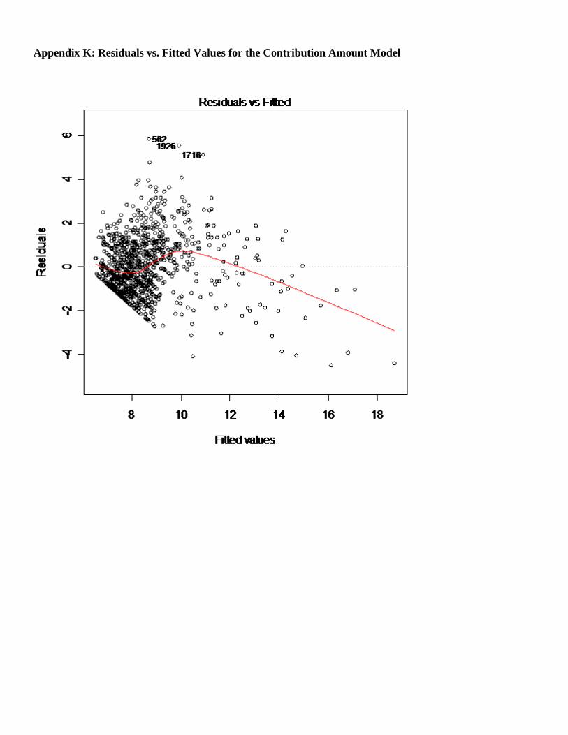
Appendix K: Residuals vs. Fitted Values for the Contribution Amount Model