regression: predicting and relating quantitative featurescshalizi/uada/13/lectures/ch01.pdf ·...

10:25 Wednesday 30th January, 2013

Chapter 1

Regression: Predicting andRelating Quantitative Features

1.1 Statistics, Data Analysis, Regression

Statistics is the branch of mathematical engineering which designs and analyses meth-ods for drawing reliable inferences from imperfect data.

The subject of most sciences is some aspect of the world around us, or withinus. Psychology studies minds; geology studies the Earth’s composition and form;economics studies production, distribution and exchange; mycology studies mush-rooms. Statistics does not study the world, but some of the ways we try to under-stand the world — some of the intellectual tools of the other sciences. Its utility comesindirectly, through helping those other sciences.

This utility is very great, because all the sciences have to deal with imperfectdata. Data may be imperfect because we can only observe and record a small fractionof what is relevant; or because we can only observe indirect signs of what is trulyrelevant; or because, no matter how carefully we try, our data always contain anelement of noise. Over the last two centuries, statistics has come to handle all suchimperfections by modeling them as random processes, and probability has becomeso central to statistics that we introduce random events deliberately (as in samplesurveys).1

Statistics, then, uses probability to model inference from data. We try to math-ematically understand the properties of different procedures for drawing inferences:Under what conditions are they reliable? What sorts of errors do they make, andhow often? What can they tell us when they work? What are signs that somethinghas gone wrong? Like other branches of engineering, statistics aims not just at un-derstanding but also at improvement: we want to analyze data better, more reliably,with fewer and smaller errors, under broader conditions, faster, and with less mental

1Two excellent, but very different, histories of how statistics came to this understanding are Hacking(1990) and Porter (1986).

17

1.2. GUESSING THE VALUE OF A RANDOM VARIABLE 18

effort. Sometimes some of these goals conflict — a fast, simple method might be veryerror-prone, or only reliable under a narrow range of circumstances.

One of the things that people most often want to know about the world is howdifferent variables are related to each other, and one of the central tools statistics hasfor learning about relationships is regression.2 In your linear regression class, youlearned about how it could be used in data analysis, and learned about its properties.In this class, we will build on that foundation, extending beyond basic linear regres-sion in many directions, to answer many questions about how variables are related toeach other.

This is intimately related to prediction. Being able to make predictions isn’t theonly reason we want to understand relations between variables, but prediction testsour knowledge of relations. (If we misunderstand, we might still be able to predict,but it’s hard to see how we could understand and not be able to predict.) So beforewe go beyond linear regression, we will first look at prediction, and how to predictone variable from nothing at all. Then we will look at predictive relationships be-tween variables, and see how linear regression is just one member of a big family ofsmoothing methods, all of which are available to us.

1.2 Guessing the Value of a Random Variable

We have a quantitative, numerical variable, which we’ll imaginatively call Y . We’llsuppose that it’s a random variable, and try to predict it by guessing a single valuefor it. (Other kinds of predictions are possible — we might guess whether Y will fallwithin certain limits, or the probability that it does so, or even the whole probabilitydistribution of Y . But some lessons we’ll learn here will apply to these other kindsof predictions as well.) What is the best value to guess? More formally, what is theoptimal point forecast for Y ?

To answer this question, we need to pick a function to be optimized, whichshould measure how good our guesses are — or equivalently how bad they are, howbig an error we’re making. A reasonable start point is the mean squared error:

MSE(a)⌘ Eî(Y � a)2ó

(1.1)

2The origin of the name is instructive. It comes from 19th century investigations into the relationshipbetween the attributes of parents and their children. People who are taller (heavier, faster, . . . ) thanaverage tend to have children who are also taller than average, but not quite as tall. Likewise, the childrenof unusually short parents also tend to be closer to the average, and similarly for other traits. This came tobe called “regression towards the mean”, or even “regression towards mediocrity”; hence the line relatingthe average height (or whatever) of children to that of their parents was “the regression line”, and the wordstuck.


19 1.3. THE REGRESSION FUNCTION

So we’d like to find the value r where MSE(a) is smallest.

MSE(a) = Eî(Y � a)2ó

(1.2)

= (E[Y � a])2+Var[Y � a] (1.3)= (E[Y � a])2+Var[Y ] (1.4)= (E[Y ]� a)2+Var[Y ] (1.5)

dMSEda

= �2 (E[Y ]� a)+ 0 (1.6)

2(E[Y ]� r ) = 0 (1.7)r = E[Y ] (1.8)

So, if we gauge the quality of our prediction by mean-squared error, the best predic-tion to make is the expected value.

1.2.1 Estimating the Expected ValueOf course, to make the prediction E[Y ] we would have to know the expected valueof Y . Typically, we do not. However, if we have sampled values, y1, y2, . . . yn , we canestimate the expectation from the sample mean:

br ⌘ 1n

nXi=1

yi (1.9)

If the samples are independent and identically distributed (IID), then the law of largenumbers tells us that

br ! E[Y ] = r (1.10)

and the central limit theorem tells us something about how fast the convergence is(namely the squared error will typically be about Var[Y ]/n).

Of course the assumption that the yi come from IID samples is a strong one, butwe can assert pretty much the same thing if they’re just uncorrelated with a commonexpected value. Even if they are correlated, but the correlations decay fast enough, allthat changes is the rate of convergence. So “sit, wait, and average” is a pretty reliableway of estimating the expectation value.

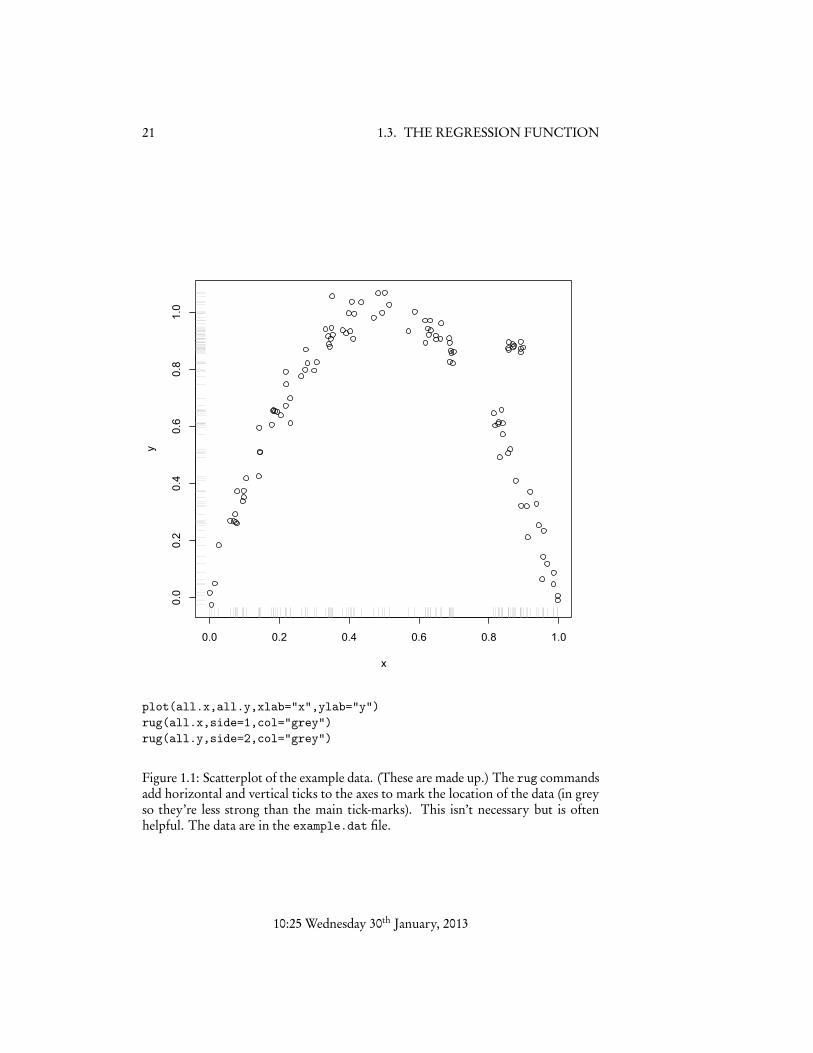
1.3 The Regression FunctionOf course, it’s not very useful to predict just one number for a variable. Typically,we have lots of variables in our data, and we believe they are related somehow. Forexample, suppose that we have data on two variables, X and Y , which might looklike Figure 1.1. The feature Y is what we are trying to predict, a.k.a. the dependentvariable or output or response, and X is the predictor or independent variableor covariate or input. Y might be something like the profitability of a customerand X their credit rating, or, if you want a less mercenary example, Y could besome measure of improvement in blood cholesterol and X the dose taken of a drug.


1.3. THE REGRESSION FUNCTION 20

Typically we won’t have just one input feature X but rather many of them, but thatgets harder to draw and doesn’t change the points of principle.

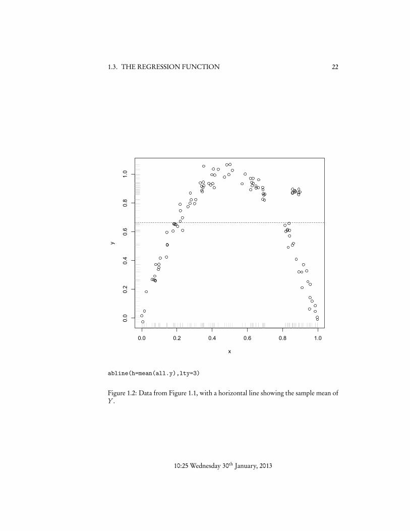
Figure 1.2 shows the same data as Figure 1.1, only with the sample mean addedon. This clearly tells us something about the data, but also it seems like we should beable to do better — to reduce the average error — by using X , rather than by ignoringit.

Let’s say that the we want our prediction to be a function of X , namely f (X ).What should that function be, if we still use mean squared error? We can work thisout by using the law of total expectation, i.e., the fact that E[U ] = E[E[U |V ]] forany random variables U and V .

MSE( f (X )) = Eî(Y � f (X ))2ó

(1.11)

= Eî

Eî(Y � f (X ))2|Xóó

(1.12)

= Eî

Var[Y |X ]+ (E[Y � f (X )|X ])2ó

(1.13)

When we want to minimize this, the first term inside the expectation doesn’t dependon our prediction, and the second term looks just like our previous optimizationonly with all expectations conditional on X , so for our optimal function r (x) we get

r (x) = E[Y |X = x] (1.14)

In other words, the (mean-squared) optimal conditional prediction is just the condi-tional expected value. The function r (x) is called the regression function. This iswhat we would like to know when we want to predict Y .

1.3.1 Some DisclaimersIt’s important to be clear on what is and is not being assumed here. Talking about Xas the “independent variable” and Y as the “dependent” one suggests a causal model,which we might write

Y r (X )+ ✏ (1.15)

where the direction of the arrow, , indicates the flow from causes to effects, and✏ is some noise variable. If the gods of inference are very, very kind, then ✏ wouldhave a fixed distribution, independent of X , and we could without loss of generalitytake it to have mean zero. (“Without loss of generality” because if it has a non-zeromean, we can incorporate that into r (X ) as an additive constant.) However, no suchassumption is required to get Eq. 1.14. It works when predicting effects from causes,or the other way around when predicting (or “retrodicting”) causes from effects, orindeed when there is no causal relationship whatsoever between X and Y 3. It isalways true that

Y |X = r (X )+ ⌘(X ) (1.16)

where ⌘(X ) is a noise variable with mean zero, but as the notation indicates thedistribution of the noise generally depends on X .

3We will cover causal inference in considerable detail in Part III.


21 1.3. THE REGRESSION FUNCTION

0.0 0.2 0.4 0.6 0.8 1.0

0.0

0.2

0.4

0.6

0.8

1.0

x

y

plot(all.x,all.y,xlab="x",ylab="y")rug(all.x,side=1,col="grey")rug(all.y,side=2,col="grey")

Figure 1.1: Scatterplot of the example data. (These are made up.) The rug commandsadd horizontal and vertical ticks to the axes to mark the location of the data (in greyso they’re less strong than the main tick-marks). This isn’t necessary but is oftenhelpful. The data are in the example.dat file.


1.3. THE REGRESSION FUNCTION 22

0.0 0.2 0.4 0.6 0.8 1.0

0.0

0.2

0.4

0.6

0.8

1.0

x

y

abline(h=mean(all.y),lty=3)

Figure 1.2: Data from Figure 1.1, with a horizontal line showing the sample mean ofY .


23 1.4. ESTIMATING THE REGRESSION FUNCTION

It’s also important to be clear that when we find the regression function is a con-stant, r (x) = r0 for all x, that this does not mean that X and Y are statisticallyindependent. If they are independent, then the regression function is a constant, butturning this around is the logical fallacy of “affirming the consequent”4.

1.4 Estimating the Regression FunctionWe want to find the regression function r (x) = E[Y |X = x], and what we’ve gotis a big set of training examples, of pairs (x1, y1), (x2, y2), . . . (xn , yn). How should weproceed?

If X takes on only a finite set of values, then a simple strategy is to use the condi-tional sample means:

br (x) = 1#{i : xi = x}X

i :xi=xyi (1.17)

By the same kind of law-of-large-numbers reasoning as before, we can be confidentthat br (x)! E[Y |X = x].

Unfortunately, this only works if X has only a finite set of values. If X is contin-uous, then in general the probability of our getting a sample at any particular valueis zero, is the probability of getting multiple samples at exactly the same value of x.This is a basic issue with estimating any kind of function from data — the functionwill always be undersampled, and we need to fill in between the values we see. Wealso need to somehow take into account the fact that each yi is a sample from theconditional distribution of Y |X = xi , and so is not generally equal to E

⇥Y |X = xi⇤

.So any kind of function estimation is going to involve interpolation, extrapolation,and smoothing.

Different methods of estimating the regression function — different regressionmethods, for short — involve different choices about how we interpolate, extrapolateand smooth. This involves our making a choice about how to approximate r (x) bya limited class of functions which we know (or at least hope) we can estimate. Thereis no guarantee that our choice leads to a good approximation in the case at hand,though it is sometimes possible to say that the approximation error will shrink aswe get more and more data. This is an extremely important topic and deserves anextended discussion, coming next.

1.4.1 The Bias-Variance Tradeoff

Suppose that the true regression function is r (x), but we use the function br to makeour predictions. Let’s look at the mean squared error at X = x in a slightly differentway than before, which will make it clearer what happens when we can’t use r to

4As in combining the fact that all human beings are featherless bipeds, and the observation that acooked turkey is a featherless biped, to conclude that cooked turkeys are human beings. An econome-trician stops there; an econometrician who wants to be famous writes a best-selling book about how thisproves that Thanksgiving is really about cannibalism.


1.4. ESTIMATING THE REGRESSION FUNCTION 24

make predictions. We’ll begin by expanding (Y � br (x))2, since the MSE at x is justthe expectation of this.

(Y � br (x))2 (1.18)= (Y � r (x)+ r (x)� br (x))2= (Y � r (x))2+ 2(Y � r (x))(r (x)� br (x))+ (r (x)� br (x))2 (1.19)

We saw above (Eq. 1.16) that Y � r (x) = ⌘, a random variable which has expectationzero (and is uncorrelated with x). When we take the expectation of Eq. 1.19, nothinghappens to the last term (since it doesn’t involve any random quantities); the middleterm goes to zero (because E[Y � r (x)] = E[⌘] = 0), and the first term becomes thevariance of ⌘. This depends on x, in general, so let’s call it �2

x . We have

MSE(br (x)) = �2x + ((r (x)� br (x))2 (1.20)

The �2x term doesn’t depend on our prediction function, just on how hard it is, in-

trinsically, to predict Y at X = x. The second term, though, is the extra error weget from not knowing r . (Unsurprisingly, ignorance of r cannot improve our pre-dictions.) This is our first bias-variance decomposition: the total MSE at x is de-composed into a (squared) bias r (x)� br (x), the amount by which our predictionsare systematically off, and a variance �2

x , the unpredictable, “statistical” fluctuationaround even the best prediction.

All of the above assumes that br is a single fixed function. In practice, of course,br is something we estimate from earlier data. But if those data are random, the exactregression function we get is random too; let’s call this random function cRn , wherethe subscript reminds us of the finite amount of data we used to estimate it. What wehave analyzed is really MSE(cRn(x)|cRn = br ), the mean squared error conditional on aparticular estimated regression function. What can we say about the prediction errorof the method, averaging over all the possible training data sets?

MSE(cRn(x)) = Eh(Y �cRn(X ))

2|X = xi

(1.21)

= Eh

Eh(Y �cRn(X ))

2|X = x,cRn = bri|X = xi

(1.22)

= Eh�2

x + (r (x)�cRn(x))2|X = xi

(1.23)

= �2x +Eh(r (x)�cRn(x))

2|X = xi

(1.24)

= �2x +Eh(r (x)�EhcRn(x)i+EhcRn(x)i�cRn(x))

2i

(1.25)

= �2x +⇣

r (x)�EhcRn(x)i⌘2+VarhcRn(x)i

(1.26)

This is our second bias-variance decomposition — I pulled the same trick as before,adding and subtract a mean inside the square. The first term is just the varianceof the process; we’ve seen that before and isn’t, for the moment, of any concern.The second term is the bias in using cRn to estimate r — the approximation bias or



approximation error. The third term, though, is the variance in our estimate of theregression function. Even if we have an unbiased method (r (x) = E

hcRn(x)i

), if thereis a lot of variance in our estimates, we can expect to make large errors.

The approximation bias has to depend on the true regression function. For ex-ample, if EhcRn(x)i= 42+ 37x, the error of approximation will be zero if r (x) =

42+ 37x, but it will be larger and x-dependent if r (x) = 0. However, there are flexi-ble methods of estimation which will have small approximation biases for all r in abroad range of regression functions. The catch is that, at least past a certain point,decreasing the approximation bias can only come through increasing the estimationvariance. This is the bias-variance trade-off. However, nothing says that the trade-off has to be one-for-one. Sometimes we can lower the total error by introducingsome bias, since it gets rid of more variance than it adds approximation error. Thenext section gives an example.

In general, both the approximation bias and the estimation variance depend on n.A method is consistent5 when both of these go to zero as n! 0 — that is, if we re-cover the true regression function as we get more and more data.6 Again, consistencydepends on how well the method matches the actual data-generating process, not juston the method, and again, there is a bias-variance trade-off. There can be multipleconsistent methods for the same problem, and their biases and variances don’t haveto go to zero at the same rates.

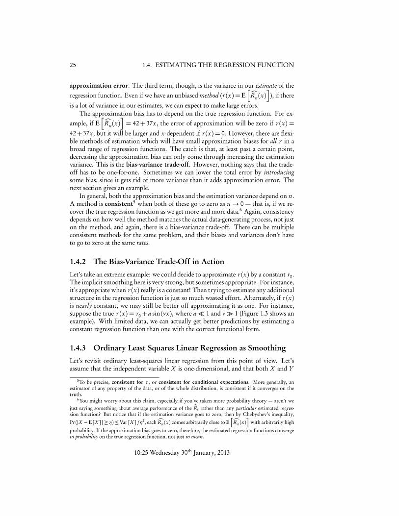
1.4.2 The Bias-Variance Trade-Off in ActionLet’s take an extreme example: we could decide to approximate r (x) by a constant r0.The implicit smoothing here is very strong, but sometimes appropriate. For instance,it’s appropriate when r (x) really is a constant! Then trying to estimate any additionalstructure in the regression function is just so much wasted effort. Alternately, if r (x)is nearly constant, we may still be better off approximating it as one. For instance,suppose the true r (x) = r0+ a sin (⌫x), where a⌧ 1 and ⌫ � 1 (Figure 1.3 shows anexample). With limited data, we can actually get better predictions by estimating aconstant regression function than one with the correct functional form.

1.4.3 Ordinary Least Squares Linear Regression as SmoothingLet’s revisit ordinary least-squares linear regression from this point of view. Let’sassume that the independent variable X is one-dimensional, and that both X and Y

5To be precise, consistent for r , or consistent for conditional expectations. More generally, anestimator of any property of the data, or of the whole distribution, is consistent if it converges on thetruth.

6You might worry about this claim, especially if you’ve taken more probability theory — aren’t wejust saying something about average performance of the bR, rather than any particular estimated regres-sion function? But notice that if the estimation variance goes to zero, then by Chebyshev’s inequality,Pr (|X �E[X ] |� ⌘)Var[X ]/⌘2, each”Rn (x) comes arbitrarily close to E

h”Rn (x)i

with arbitrarily highprobability. If the approximation bias goes to zero, therefore, the estimated regression functions convergein probability on the true regression function, not just in mean.



0.0 0.2 0.4 0.6 0.8 1.0

0.0

0.5

1.0

1.5

2.0

x

y

ugly.func = function(x) {1 + 0.01*sin(100*x)}

r = runif(100); y = ugly.func(r) + rnorm(length(r),0,0.5)

plot(r,y,xlab="x",ylab="y"); curve(ugly.func,add=TRUE)

abline(h=mean(y),col="red")

sine.fit = lm(y ~ 1+ sin(100*r))

curve(sine.fit$coefficients[1]+sine.fit$coefficients[2]*sin(100*x),

col="blue",add=TRUE)

Figure 1.3: A rapidly-varying but nearly-constant regression function; Y = 1 +0.01 sin100x + ✏, with ✏ ⇠ N (0,0.1). (The x values are uniformly distributed be-tween 0 and 1.) Red: constant line at the sample mean. Blue: estimated function ofthe same form as the true regression function, i.e., r0 + a sin100x. If the data set issmall enough, the constant actually generalizes better — the bias of using the wrongfunctional form is smaller than the additional variance from the extra degrees of free-dom. Here, the root-mean-square (RMS) error of the constant on new data is 0.50,while that of the estimated sine function is 0.51 — using the right function actuallyhurts us!



are centered (i.e. have mean zero) — neither of these assumptions is really necessary,but they reduce the book-keeping.

We choose to approximate r (x) by ↵+�x, and ask for the best values a, b of thoseconstants. These will be the ones which minimize the mean-squared error.

M SE(↵,�) = Eî(Y �↵��X )2ó

(1.27)

= Eî(Y �↵��X )2|X

ó(1.28)

= Eî

Var[Y |X ]+ (E[Y �↵��X |X ])2ó

(1.29)

= E[Var[Y |X ]]+Eî(E[Y �↵��X |X ])2

ó(1.30)

The first term doesn’t depend on ↵ or �, so we can drop it for purposes of optimiza-tion. Taking derivatives, and then brining them inside the expectations,

@ M SE@ ↵

= E[2(Y �↵��X )(�1)] (1.31)

E[Y � a� bX ] = 0 (1.32)a = E[Y ]� bE[X ] = 0 (1.33)

using the fact that X and Y are centered; and,

@ M SE@ �

= E[2(Y �↵��X )(�X )] (1.34)

E[X Y ]� bEî

X 2ó= 0 (1.35)

b =Cov[X ,Y ]

Var[X ](1.36)

again using the centering of X and Y . That is, the mean-squared optimal linear pre-diction is

r (x) = xCov[X ,Y ]

Var[X ](1.37)

Now, if we try to estimate this from data, there are (at least) two approaches. Oneis to replace the true population values of the covariance and the variance with theirsample values, respectively

1n

Xi

yi xi (1.38)

and1n

Xi

x2i (1.39)

(again, assuming centering). The other is to minimize the residual sum of squares,

RSS(↵,�)⌘X

i

�yi �↵��xi�2 (1.40)



You may or may not find it surprising that both approaches lead to the same answer:

ba = 0 (1.41)

bb =P

i yi xiPi x2

i

(1.42)

Provided that Var[X ] > 0, this will converge with IID samples, so we have a consis-tent estimator.7

We are now in a position to see how the least-squares linear regression model isreally a smoothing of the data. Let’s write the estimated regression function explicitlyin terms of the training data points.

br (x) = bb x (1.43)

= xP

i yi xiPi x2

i

(1.44)

=X

iyi

xiPj x2

j

x (1.45)

=X

iyi

xi

ns2X

x (1.46)

where s2X is the sample variance of X . In words, our prediction is a weighted average

of the observed values yi of the dependent variable, where the weights are propor-tional to how far xi is from the center (relative to the variance), and proportionalto the magnitude of x. If xi is on the same side of the center as x, it gets a positiveweight, and if it’s on the opposite side it gets a negative weight.

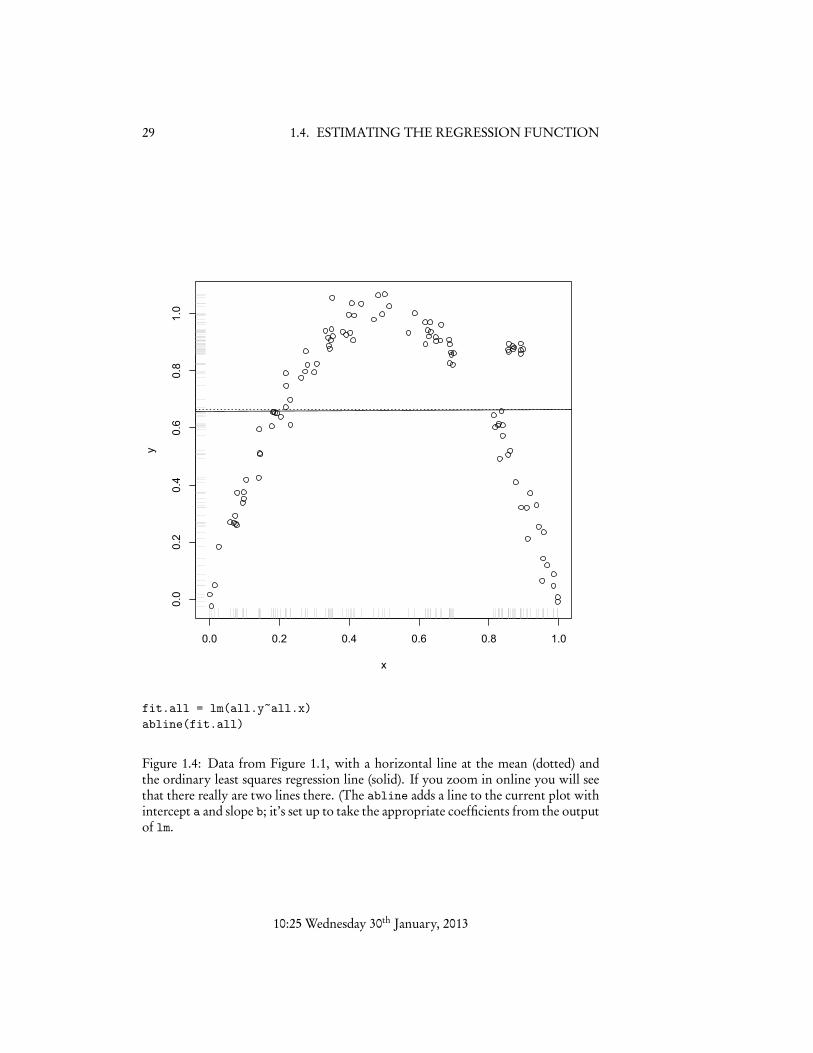
Figure 1.4 shows the data from Figure 1.1 with the least-squares regression lineadded. It will not escape your notice that this is very, very slightly different from theconstant regression function; the coefficient on X is 6.3⇥10�3. Visually, the problemis that there should be a positive slope in the left-hand half of the data, and a negativeslope in the right, but the slopes are the densities are balanced so that the best singleslope is zero.8

Mathematically, the problem arises from the peculiar way in which least-squareslinear regression smoothes the data. As I said, the weight of a data point depends onhow far it is from the center of the data, not how far it is from the point at which we aretrying to predict. This works when r (x) really is a straight line, but otherwise — e.g.,here — it’s a recipe for trouble. However, it does suggest that if we could somehowjust tweak the way we smooth the data, we could do better than linear regression.

7Eq. 1.41 may look funny, but remember that we’re assuming X and Y have been centered. Centeringdoesn’t change the slope of the least-squares line but does change the intercept; if we go back to the un-centered variables the intercept becomes Y � bbX , where the bar denotes the sample mean.

8The standard test of whether this coefficient is zero is about as far from rejecting the null hypothesisas you will ever see, p = 0.95. Remember this the next time you look at regression output.



0.0 0.2 0.4 0.6 0.8 1.0

0.0

0.2

0.4

0.6

0.8

1.0

x

y

fit.all = lm(all.y~all.x)abline(fit.all)

Figure 1.4: Data from Figure 1.1, with a horizontal line at the mean (dotted) andthe ordinary least squares regression line (solid). If you zoom in online you will seethat there really are two lines there. (The abline adds a line to the current plot withintercept a and slope b; it’s set up to take the appropriate coefficients from the outputof lm.


1.5. LINEAR SMOOTHERS 30

1.5 Linear SmoothersThe sample mean and the linear regression line are both special cases of linear smoothers,which are estimates of the regression function with the following form:

br (x) =X

iyi bw(xi , x) (1.47)

The sample mean is the special case where bw(xi , x) = 1/n, regardless of what xiand x are.

Ordinary linear regression is the special case where bw(xi , x) = (xi/ns2X )x.

Both of these, as remarked, ignore how far xi is from x.

1.5.1 k-Nearest-Neighbor RegressionAt the other extreme, we could do nearest-neighbor regression:

bw(xi , x) =⇢

1 xi nearest neighbor of x0 otherwise (1.48)

This is very sensitive to the distance between xi and x. If r (x) does not change toorapidly, and X is pretty thoroughly sampled, then the nearest neighbor of x amongthe xi is probably close to x, so that r (xi ) is probably close to r (x). However, yi =r (xi )+noise, so nearest-neighbor regression will include the noise into its prediction.We might instead do k-nearest neighbor regression,

bw(xi , x) =⇢

1/k xi one of the k nearest neighbors of x0 otherwise (1.49)

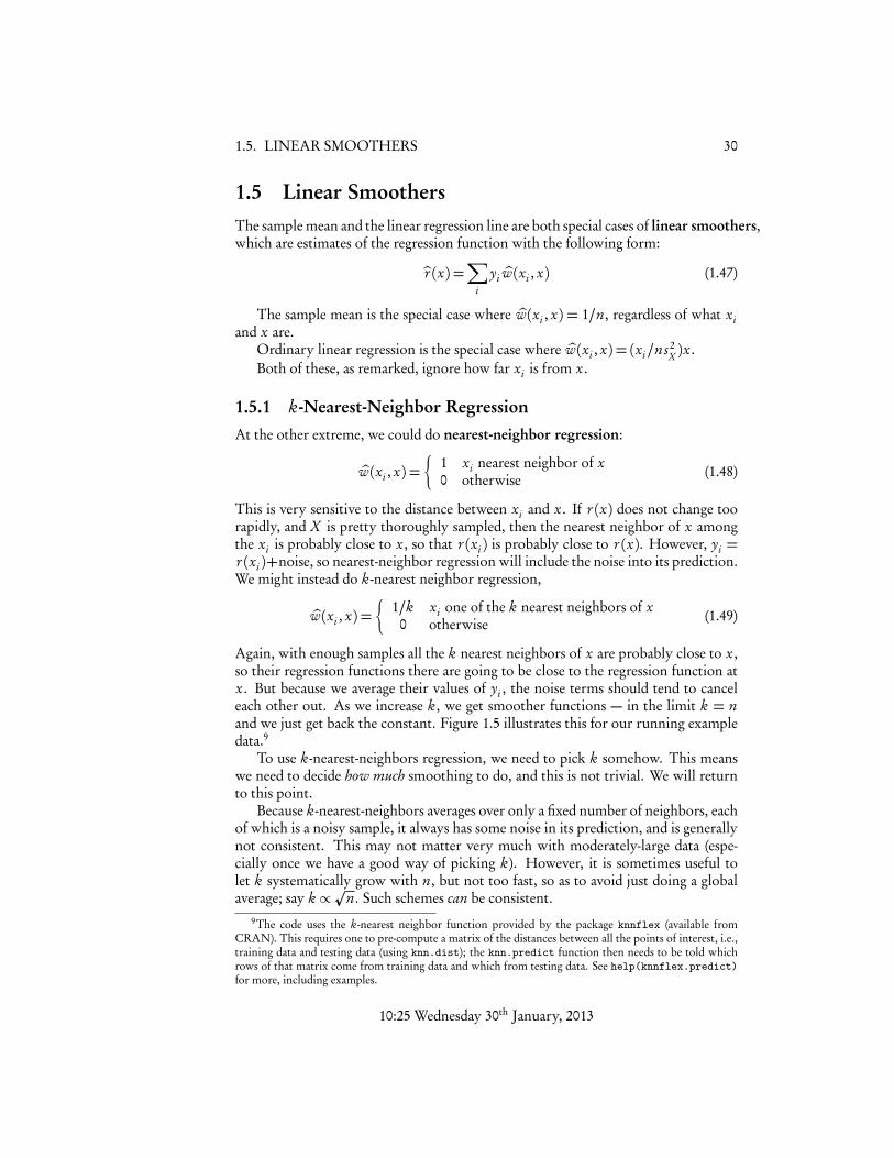
Again, with enough samples all the k nearest neighbors of x are probably close to x,so their regression functions there are going to be close to the regression function atx. But because we average their values of yi , the noise terms should tend to canceleach other out. As we increase k, we get smoother functions — in the limit k = nand we just get back the constant. Figure 1.5 illustrates this for our running exampledata.9

To use k-nearest-neighbors regression, we need to pick k somehow. This meanswe need to decide how much smoothing to do, and this is not trivial. We will returnto this point.

Because k-nearest-neighbors averages over only a fixed number of neighbors, eachof which is a noisy sample, it always has some noise in its prediction, and is generallynot consistent. This may not matter very much with moderately-large data (espe-cially once we have a good way of picking k). However, it is sometimes useful tolet k systematically grow with n, but not too fast, so as to avoid just doing a globalaverage; say k /pn. Such schemes can be consistent.

9The code uses the k-nearest neighbor function provided by the package knnflex (available fromCRAN). This requires one to pre-compute a matrix of the distances between all the points of interest, i.e.,training data and testing data (using knn.dist); the knn.predict function then needs to be told whichrows of that matrix come from training data and which from testing data. See help(knnflex.predict)for more, including examples.


31 1.5. LINEAR SMOOTHERS

0.0 0.2 0.4 0.6 0.8 1.0

0.0

0.2

0.4

0.6

0.8

1.0

x

y

library(knnflex)

all.dist = knn.dist(c(all.x,seq(from=0,to=1,length.out=100)))

all.nn1.predict = knn.predict(1:110,111:210,all.y,all.dist,k=1)

abline(h=mean(all.y),lty=2)

lines(seq(from=0,to=1,length.out=100),all.nn1.predict,col="blue")


lines(seq(from=0,to=1,length.out=100),all.nn3.predict,col="red")


lines(seq(from=0,to=1,length.out=100),all.nn5.predict,col="green")


lines(seq(from=0,to=1,length.out=100),all.nn20.predict,col="purple")

Figure 1.5: Data points from Figure 1.1 with horizontal dashed line at the mean andthe k-nearest-neighbor regression curves for k = 1 (blue), k = 3 (red), k = 5 (green)and k = 20 (purple). Note how increasing k smoothes out the regression line, andpulls it back towards the mean. (k = 100 would give us back the dashed horizontalline.)



1.5.2 Kernel SmoothersChanging k in a k-nearest-neighbors regression lets us change how much smoothingwe’re doing on our data, but it’s a bit awkward to express this in terms of a numberof data points. It feels like it would be more natural to talk about a range in theindependent variable over which we smooth or average. Another problem with k-NN regression is that each testing point is predicted using information from only afew of the training data points, unlike linear regression or the sample mean, whichalways uses all the training data. If we could somehow use all the training data, butin a location-sensitive way, that would be nice.

There are several ways to do this, as we’ll see, but a particularly useful one is to usea kernel smoother, a.k.a. kernel regression or Nadaraya-Watson regression. Tobegin with, we need to pick a kernel function10 K(xi , x)which satisfies the followingproperties:

1. K(xi , x)� 0

2. K(xi , x) depends only on the distance xi � x, not the individual arguments

3.R

xK(0, x)d x = 0

4. 0<R

x2K(0, x)d x <1These conditions together (especially the last one) imply that K(xi , x)! 0 as |xi �x| ! 1. Two examples of such functions are the density of the Unif(�h/2, h/2)distribution, and the density of the standard Gaussian N (0,

ph) distribution. Here

h can be any positive number, and is called the bandwidth.The Nadaraya-Watson estimate of the regression function is

br (x) =X

iyi

K(xi , x)Pj K(xj , x)

(1.50)

i.e., in terms of Eq. 1.47,

bw(xi , x) =K(xi , x)Pj K(xj , x)

(1.51)

(Notice that here, as in k-NN regression, the sum of the weights is always 1. Why?)11

What does this achieve? Well, K(xi , x) is large if xi is close to x, so this will placea lot of weight on the training data points close to the point where we are trying topredict. More distant training points will have smaller weights, falling off towardszero. If we try to predict at a point x which is very far from any of the trainingdata points, the value of K(xi , x) will be small for all xi , but it will typically be much,

10There are many other mathematical objects which are also called “kernels”. Some of these meaningsare related, but not all of them. (Cf. “normal”.)

11What do we do if K(xi , x) is zero for some xi ? Nothing; they just get zero weight in the average.What do we do if all the K(xi , x) are zero? Different people adopt different conventions; popular onesare to return the global, unweighted mean of the yi , to do some sort of interpolation from regions wherethe weights are defined, and to throw up our hands and refuse to make any predictions (computationally,return NA).


33 1.5. LINEAR SMOOTHERS

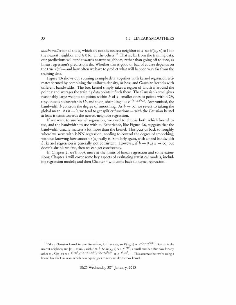
much smaller for all the xi which are not the nearest neighbor of x, so bw(xi , x)⇡ 1 forthe nearest neighbor and ⇡ 0 for all the others.12 That is, far from the training data,our predictions will tend towards nearest neighbors, rather than going off to ±1, aslinear regression’s predictions do. Whether this is good or bad of course depends onthe true r (x)— and how often we have to predict what will happen very far from thetraining data.

Figure 1.6 shows our running example data, together with kernel regression esti-mates formed by combining the uniform-density, or box, and Gaussian kernels withdifferent bandwidths. The box kernel simply takes a region of width h around thepoint x and averages the training data points it finds there. The Gaussian kernel givesreasonably large weights to points within h of x, smaller ones to points within 2h,tiny ones to points within 3h, and so on, shrinking like e�(x�xi )2/2h . As promised, thebandwidth h controls the degree of smoothing. As h !1, we revert to taking theglobal mean. As h! 0, we tend to get spikier functions — with the Gaussian kernelat least it tends towards the nearest-neighbor regression.

If we want to use kernel regression, we need to choose both which kernel touse, and the bandwidth to use with it. Experience, like Figure 1.6, suggests that thebandwidth usually matters a lot more than the kernel. This puts us back to roughlywhere we were with k-NN regression, needing to control the degree of smoothing,without knowing how smooth r (x) really is. Similarly again, with a fixed bandwidthh, kernel regression is generally not consistent. However, if h ! 0 as n !1, butdoesn’t shrink too fast, then we can get consistency.

In Chapter 2, we’ll look more at the limits of linear regression and some exten-sions; Chapter 3 will cover some key aspects of evaluating statistical models, includ-ing regression models; and then Chapter 4 will come back to kernel regression.

12Take a Gaussian kernel in one dimension, for instance, so K(xi , x) / e�(xi�x)2/2h2. Say xi is the

nearest neighbor, and |xi � x|= L, with L� h. So K(xi , x)/ e�L2/2h2, a small number. But now for any

other xj , K(xi , x) / e�L2/2h2 e�(x j�xi )L/2h2e�(x j�xi )2/2h2 ⌧ e�L2/2h2

. — This assumes that we’re using akernel like the Gaussian, which never quite goes to zero, unlike the box kernel.



0.0 0.2 0.4 0.6 0.8 1.0

0.0

0.2

0.4

0.6

0.8

1.0

x

y

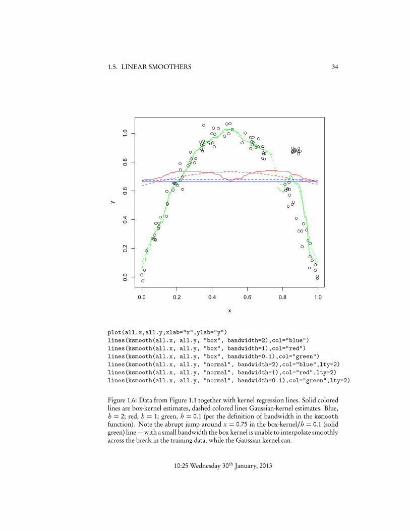
plot(all.x,all.y,xlab="x",ylab="y")lines(ksmooth(all.x, all.y, "box", bandwidth=2),col="blue")lines(ksmooth(all.x, all.y, "box", bandwidth=1),col="red")lines(ksmooth(all.x, all.y, "box", bandwidth=0.1),col="green")lines(ksmooth(all.x, all.y, "normal", bandwidth=2),col="blue",lty=2)lines(ksmooth(all.x, all.y, "normal", bandwidth=1),col="red",lty=2)lines(ksmooth(all.x, all.y, "normal", bandwidth=0.1),col="green",lty=2)

Figure 1.6: Data from Figure 1.1 together with kernel regression lines. Solid coloredlines are box-kernel estimates, dashed colored lines Gaussian-kernel estimates. Blue,h = 2; red, h = 1; green, h = 0.1 (per the definition of bandwidth in the ksmoothfunction). Note the abrupt jump around x = 0.75 in the box-kernel/h = 0.1 (solidgreen) line — with a small bandwidth the box kernel is unable to interpolate smoothlyacross the break in the training data, while the Gaussian kernel can.


35 1.6. EXERCISES

1.6 ExercisesNot to hand in.

1. Suppose we use the mean absolute error instead of the mean squared error:

MAE(a) = E[|Y � a|] (1.52)

Is this also minimized by taking a = E[Y ]? If not, what value r̃ minimizes theMAE? Should we use MSE or MAE to measure error?

2. Derive Eqs. 1.41 and 1.42 by minimizing Eq. 1.40.

3. What does it mean for Gaussian kernel regression to approach nearest-neighborregression as h ! 0? Why does it do so? Is this true for all kinds of kernelregression?

4. COMPUTING The file ckm.csv on the class website13 contains data from a fa-mous study on the “diffusion of innovations”, in this case, the adoption of tetra-cycline, a then-new antibiotic, among doctors in four cities in Illinois in the1950s. In particular, the column adoption_date records how many monthsafter the beginning of the study each doctor surveyed began prescribing tetra-cycline. Note that some doctors did not do so before the study ended (thesehave an adoption date of Inf, infinity), and this information is not availablefor others (NA).

(a) Load the data as a data-frame called ckm.(b) What does

adopters <- sapply(1:17, function(y) { sum(na.omit(ckm$adoption_date) <= y) } )

do? Why 17?(c) Plot the number of doctors who have already adopted tetracycline at the

start of each month against the number of new adopters that month. Thisshould look somewhat like a sparser version of the scatter-plot used as arunning example in this chapter. Hints: diff, plot.

(d) Linearly regress the number of new adopters against the number of adopters.Add the regression line to your scatterplot. It should suggest that increas-ing the number of doctors who have adopted the drug strictly decreasesthe number who will adopt.

(e) Add Gaussian kernel smoothing lines to your scatterplot, as in Figure 1.6.Do these suggest that the relationship is monotonic?

(f) Plot the residuals of the linear regression against the predictor variable.(Hint: residuals.) Do the residuals look independent of the predictor?What happens if you kernel smooth the residuals?

13Slightly modified from http://moreno.ss.uci.edu/data.html to fit R conventions.


regression: predicting and relating quantitative featurescshalizi/uada/13/lectures/ch01.pdf ·...

Documents