HAL Id: hal-01081557https://hal.archives-ouvertes.fr/hal-01081557

Submitted on 9 Nov 2014

HAL is a multi-disciplinary open accessarchive for the deposit and dissemination of sci-entific research documents, whether they are pub-lished or not. The documents may come fromteaching and research institutions in France orabroad, or from public or private research centers.

L’archive ouverte pluridisciplinaire HAL, estdestinée au dépôt et à la diffusion de documentsscientifiques de niveau recherche, publiés ou non,émanant des établissements d’enseignement et derecherche français ou étrangers, des laboratoirespublics ou privés.

PREDICTING HOSPITAL LENGTH OF STAY USINGREGRESSION MODELS: APPLICATION TO

EMERGENCY DEPARTMENTCatherine Combes, Farid Kadri, Sondès Chaabane

To cite this version:Catherine Combes, Farid Kadri, Sondès Chaabane. PREDICTING HOSPITAL LENGTH OF STAYUSING REGRESSION MODELS: APPLICATION TO EMERGENCY DEPARTMENT. 10ème Con-férence Francophone de Modélisation, Optimisation et Simulation- MOSIM’14, Nov 2014, Nancy,France. �hal-01081557�

PREDICTING HOSPITAL LENGTH OF STAY USING REGRESSION MODELS: APPLICATION TO EMERGENCY DEPARTMENT

Catherine COMBES1

Farid KADRI 2,3, Sondès CHAABANE2,3

ABSTRACT: Increasing healthcare costs motivate the search for ways to increase care efficiency. In this paper, we present a novel methodological framework based on predictive data mining approach to estimate the LOS (Length Of Stay) in an emergency department (ED). We use supervised learning that the goal is to build concise models in terms of predictor features. The aim is to identify the factors (variables) characterizing the LOS in EDs in order to propose models to predict the LOS. We identified two models based on linear regression. These models are validated and were successfully applied to the classification and prediction of the LOS in the pediatric emergency department (PED) at Lille regional hospital centre, France. KEYWORDS: Emergency department, healthcare modelling, regressions, LOS forecast

1 INTRODUCTION

Nowadays, with the growing demand for emergency medical care (Kadri et al., 2014a,b), emergency depart-ments (EDs) need information to manage this patient influx and make decisions (Kadri et al., 2014c). The objective is to propose a Decision Support System (DSS) based on a data mining approaches, in order to support operational and tactical decisions. For planning and logistic purposes, it is of interest to see prediction esti-mates, to forecast the class of new clients; to have time-based forecasts and to find the variables that explain the ED behavior. For management, it is relevant to find patterns among care consumption, available from the care services. Organizations must systematically acquire the information needed to make decisions and to evalu-ate the effects and consequences of these decisions. To fully explore the opportunities for our approach, we propose a modelling environment based on data ware-housing and data mining approaches (Figure 1). This allows one to manage the resources, to elaborate medico-social resource planning and to eventually simulate them in order to evaluate their performances.

The main aim of the proposed DSS is to improve the decisional performances by discovering some links be-tween data and checking hypotheses (observations).

The objective is to prove the contribution of data mining approach for health care management. The application concerns the prediction of the length of stay (LOS) for patients admitted to hospital emergency department.

Data are been collected from the database of Pediatric Emergency Department in Lille regional hospital centre, France, The dataset includes 12,498 patients on a period of 6 months.

Figure 1: Modelling environment.

During the last decades, several applications for Machine Learning (ML) are used and the most significant of which is predictive data mining and concerns classifica-tion problems. Classification is one of the most common learning models in data mining. The aim is to identify a model in order to predict future behaviors through classi-fying database records into a number of predefined clas-ses/groups based on certain criteria. The resulting classi-fier is then used to assign class labels to the testing in-stances where the values of the predictor features are known, but the value of the class label is unknown. The most common tools used for classification are linear regression, neural networks, decision trees, if-then-else rules, Bayesian networks, Naive Bayes classifiers, neural networks, Super vectors machines and regression (tree regression, logistic regression, support vector regres-sion…). Using regression includes curve fitting, prediction (fore-casting), modeling of causal relationships, and testing

1PRES Lyon, Hubert Curien Laboratory - University Jean-Monnet, Saint-Etienne, France catherine.combes@univ-st-etienne.fr

2Univ. Lille Nord de France, F-59000 Lille, France 3TEMPO Lab., PSI Team, F-59313 Valenciennes, France

Farid.kadri@univ-valenciennes.fr sondes.chaabane@univ-valenciennes.fr

scientific hypotheses about relationships between varia-bles. Regression analysis is a method for investigating func-tional relationships among variables that is expressed in the form of an equation or a model connecting the re-sponse or dependent variable and one or more explanato-ry or predictor variables. The structure of the rest of this paper is as follows. Sec-tion 2 gives an overview of the contribution of data min-ing and presents related works. The methodological approach is described in section 3. We test the different algorithms based on regressions from data and identify the relevant variables. The proposed models and the experiments with a real case study from French Emer-gency Department are described. Conclusions and an outlook are finally presented in Section 4.

2 RELATED WORK

Data mining allows finding models and patterns from the available data. Data mining is a discipline at the interface of statistics and information technologies: databases, artificial intelligence, machine learning. Data mining includes descriptive data mining algorithms for finding interesting patterns in the data, like associations, clusters and subgroups, but also predictive data mining algo-rithms, which result in models that can be used for pre-diction and classification.

The aim of data mining is to automatically find useful information in large quantities of data. Data mining can be both predictive and descriptive: in the first case, the objective is to predict the value of a particular attribute given existing data, in the latter case the objective is to derive patterns that summarize the underlying relation-ships in the data. Data mining hence is an integral part of knowledge discovery, which is the overall process of converting raw data into knowledge through obtaining useful information from the data. In (Tan, 2007), four core data mining tasks are identi-fied:

1. Predictive modelling. The task is to build a pre-dictive model for a target variable, based of ex-planatory variables. Classification and regression are methods to predict a discrete outcome (eg. whether or not somebody will do something) cq. an extrapolation of continuous output (eg. what the future value of a measurement will be).

2. Attribute selection. Most machine learning algo-rithms allows us to learn which are the most ap-propriate attributes (predictor variables) to use for making their decisions. Most methods for attrib-ute selection involve the space of attributes for the subset that is most likely to predict the class best.

3. Association analysis. The goal is to discover pat-terns that describe strongly associated features in the data. Typically, one tries to find implication rules. An example application is the understand-ing relationships between different goods bought simultaneously in a supermarket, e.g. the pattern

that people buying milk also buy bread, or people buying beer also buy snacks.

4. Cluster analysis. The goal is to group similar ob-servations such that observations within one group are more similar to each other, and obser-vations of different groups are less similar to each other. For example, this way it is possible to find groups of customers with related behavior.

5. Anomaly detection. The task is to detect outliers, i.e. whose characteristics are significantly differ-ent from the rest of the data. A good anomaly de-tector should have a low error rate and a high de-tection rate. An example application domain is the detection of spam email.

Since last decade, many works deals with the contribu-tion of implementing information systems in health care organizations (Berg, 2001; Duan et al., 2011) in order to analyze healthcare quality indicator (Chae et al., 2003; Kadri et al., 2013).

Theoretical models are based on statistical pattern recog-nition well-described in (Jain et al., 2000; Kotsiantis, 2007; Kotsiantis et al., 2006) present interesting reviews of classification methods and combining techniques. Recently, (Esfandiari et al., 2014) present a state of art concerning 291 papers published between 1999 and 2013 from wide variety of journals such as data mining and medicine. The authors clarify medical data mining and its main goals. Five data mining approaches are considered: classification, regression, clustering, associa-tion and hybrid. We observe regarding this article that there is wide variety of applications that covered most of the medicine field but the authors focused only on a structural data.

Our paper focuses on predictive modelling. The objec-tive is to predict the LOS in the emergency department. But what are the “best” methods? Decision Trees are considered to be one of the most popular approaches and easily understood tools for rep-resenting classifiers. They can handle both nominal and numeric input attributes. Most of the algorithms (like ID3 and C4.5) require that the target attribute will have only discrete values and are less appropriate for estima-tion tasks where the goal is to predict the value of a con-tinuous attribute. Regression tree also works in a very similar fashion than classification tree. But regression trees are needed when the response variable is numeric or continuous (case of surgery duration or LOS in the emergency department). Thus regression trees are applicable for prediction type of problems as opposed to some classification tree. It might be interesting is to compare different methods (regression trees, SVM regression, logistic regression) regarding other approaches (such that decision tree, multi-layer perceptron, Bayesian networks, neural net-works…) and to study the limits of each of them regard-ing the data raw. In fact, the approach concerns the class of nonlinear predictive model which at first seems too simple to possible work, namely prediction trees. Predic-tors like linear or polynomial regression are global mod-

els, where a single predictive formula is supposed to hold over the entire data space. When the data has lots of features which interact in complicated, nonlinear ways, assembling a single global model can be very difficult and hopelessly confusing when you do succeed.

In (Austin et al., 2010), the authors compare the perfor-mances of classification techniques in order to predict the presence of coronary artery disease (CAD). The authors compared performances of logistic regression (LR), classification and regression tree (CART), multi-layer perceptron (MLP), radial basis function (RBF), and self-organizing feature maps (SOFM). Performances of classification techniques were compared using ROC curve, Hierarchical Cluster Analysis (HCA), and Multi-dimensional Scaling (MDS). The results of the classifi-cation of the top of 5 (best to worst) are:

1. MLP, 2. LR, 3. CART, 4. RBF, 5. SOFM.

Many applications show that the logistic regression gives excellent results.

(Mazzocco and Hussain, 2012) proposed prediction models based on logistic regression algorithm (Landwehr et al., 2003) to predict the diagnosis of de-mentia using variables selected either by domain experts or by a statistical driven procedure. The aim of this study is to improve on the performance of a recent application of Bayesian belief networks using an alternative ap-proach based on logistic regression.

In (Kurt et al., 2008), the authors compared the predic-tive accuracy of regression trees with that of logistic regression models for predicting in-hospital mortality in patients hospitalized with heart failure. The main conclu-sion is that Logistic regression predicted in-hospital mortality in patients hospitalized with heart failure more accurately than did the regression trees. Regression trees grown in random samples from the same data set can differ substantially from one another. The authors under-line logistic regression can take into account for the underlying linear relationships between key continuous covariates and the log-odds of in-hospital mortality.

The state of the art shows that logistic regression is a good model. In fact, logistic regression models produce probabilities rather than predictions. For each class val-ue, this technique estimates the probability that a given instance belongs to that class. It can be interesting but the main problem is the target variable should be dis-crete. But in our case, the target variable is continued. Conse-quently if we want to use logistic regression for example, we should discretize the target variable. But our objec-tive is to predict length-of-stay in the ED and not an interval of LOS. Regression analysis methods allows investigating func-tional relationships among variables that is expressed in the form of an equation or a model connecting the re-

sponse or dependent variable and one or more explanato-ry or predictor variables. But the problems caused by noisy data or outliers have been known in linear regres-sion for years. In the case of linear regression, outliers can be identified visually but it is never completely clear whether an outlier is an error or a correct value (for ex-ample in our study, the patient absconded of the Emer-gency department, and we do not have this information in our data). Although outliers dramatically affect the usual least-squares regression because the squared distance measures accentuates the influence of points far away the regression line, we decide to explore ordinary least squares (OLS) regression in order to obtain a very sim-ple model. In fact, one way of making regression more robust is to use an absolute-value measure instead of usual squared one. However, we will explore all the classification/prediction techniques in order to identify what is the “best” tech-nique.

3 METHODOLOGY

The proposed methodological framework is based on predictive modelling to approximate the LOS of a new patient at the ED. The goal is to enable prediction with a very useful model, easily understandable and usable by the hospital staff. The methodology adopted to achieve this objective is outlined Figure 2. Each step is described in the next subsections.

Figure 2: Proposed methodology.

3.1 Data description

First, the data is collected, prepared in the right format, eventually pre-visualized and fit to appropriate dimen-sions. Based on objective, we use discrete event simula-tion in order to create new variable such as “the number of patient in the system when a new patient arrived”. We want to prove the contribution in coupling simulation

Data Warehouse

Interface - queries

StatisticsReporting

OLAP Cubes Raw

Data

Data Pre-treatment

Learning set

PredictingModelling

Classification and regression

Models

Data previsualizationDeduction of new variablesIdentification of new variablesBy using Monte Carlo simulation

1. Continue target variables => Regression

2. Discretization of the targetvariable

3. Discrete Target variables => Classification

Experts’ validation

No

Motivations:Models not easily to use by the medical staffQuality of the performances of the modelsChoice: target variable to be continue value

ExploratoryData Mining

Identification relevant variables

Hierarchical analysis on variablesAttribute selectionPrincipal component analysis

Data analysisVariable analysisEmpirical distribution of the target variable

LinearRegression

models

Continue prediction by Linear regression

and data mining in order to discover new variable that it can explain the explicative variable.

3.1.1 Raw data The table 1 describes the raw data. The data come from the PED data base and concern 12, 498 patients (period January-June, 2012).

Variables Meaning Type Definition X1 Arrival Date Date Date of patient arrival

X2 Arrival time Hours Hour of patient arrival

X3 Arrival mean Numeric Arrival mean of patients (personal, fireman, mobile emergency)

X4 Adressed by

Character

Who addressed the patient to the emergency department (attending physician, internal emergency, SAMU, Centre 15...)

X5

Destination

Numeric

Destination/Orientation of patient at the end of emergency management (come back at home, hospitalization…)

X6 Age Numeric Age of patients (in months)

X7 Sex Numeric Sex of patients (1 = boy, 2 = girl)

X8 Statut Numeric 1=medical, 2= surgery

X9 CAC Numeric 3091: external care 3092: Short-term Hospitalization Unit

X10 CCMU Numeric

Clinical classification of emergency patients called CCMU (1-6)

X11 GEMSA Numeric

Multicentric Emergency Department Study Group called GEMSA (1-6)

X12 Accident Boolean 1 = yes, 0 = no

X10 Echography Boolean 1 = an echography and 0 = no echography

X11 Scanner Boolean 1= a scanner and 0 = No scanner

X12 X-Ray Boolean 1 = radiology and 0 = no radiology

X13 Comp. X-ray Boolean 1 = yes, 0 = no

X14 Biology Boolean 1 = biology test and 0 = no biology test

X15 AvisSpe Boolean Specialised advice

X16 Departure Date

Date Date of patient leaving the PED

X17 Departure time

Hours Time (hour of day) of Patient leaving the PED

Table 1. Variable description from data records coming from the emergency data base

From the raw data, we deduce news variables: � X18: Day on the week (Monday, Tuesday….), � X19: Month of the year, � X20: Season regarding the date, � X21: Period of the day (morning, afternoon,

night…) � X22: Patient’s Length of stay in the PED including

the waiting times (in minutes): LOS calculate with the variables (X1,X2) and (X14,X15).

3.1.2 Monte Carlo simulation In using Monte Carlo simulation, a model computes the number of patients present in the emergency department allowing us to deduce a new variable:

� X23: the number of patients inside of PED when a new patient arrives.

If we directly used data mining approach without previ-ously data analysis, we observe in the next paragraph that the classification by using regression methods is not easy. 3.2 Classification analysis

Our objective is to identify linear correlation between variable regarding a target variable called LOS (corre-sponding to X22). Robust estimation of LOS fluctuations is a challenging problem. The accuracy of statistical extrapolation is fairly sensitive to both model and sampling error.

3.2.1 Techniques for continue target value Only regression allows us to use continue variable of the target variable. Nine methods available in Weka1 (Hall et al., 2009) are used:

1. LR: Linear regression 2. DS (Decision Stump): Class for building and us-

ing a decision stump. Usually used in conjunction with a boosting algorithm regression (based on mean-squared error) or classification (based on entropy)

3. M5P: Induction of model trees for predicting con-tinuous classes

4. REPTree: Builds a decision/regression tree using information gain/variance and prunes it using re-duced-error pruning (with backfitting).

5. SMOreg: SVM Regression 6. IRM: Isotonic regression model 7. MLP: MultiLayer perceptron 8. PRLM: Pace regression linear models 9. KStar: K-nearest neighbors classifier (lazy)

The results are given table 2.

Methods Correla-

tion coefficient

Mean absolute

error

Root mean squared

error

Relative absolute

error (%)

Root relative squared

error (%) LR 0.5823 143.932 250.372 77.83% 81.29% DS 0.5092 155.126 265.057 83.88% 86.06% M5P 0.5893 141.762 249.004 76.66% 80.85% REPTree 0.5664 144.869 254.27 78.34% 82.56% SMOreg 0.5777 129.776 270.472 70.17% 80.56% IRM 0.5092 155.126 265.057 83.88% 86.06% MLP 0.4993 180.291 281.782 97.49% 91.49% PRLM 0.5824 143.945 250.357 77.84% 81.29% KStar 0.5438 138.687 259.180 74.99% 84.15%

Table 2: Comparisons of classifier methods with continue target variable. Total Number of Instances 12,498

1 But others free softwares can be used such as R [R, 2008], Tana-

gra [Rakotomalala, 2005]…

Classification models are not very useful when the target values are continuous. We also observe that inde-pendently of the used algorithms, we obtain quasi the same performances, but how to improve theses perfor-mances?

3.2.2 Classification with methods needing discrete target variable

Although many interesting real world domains demand for regression tools, machine learning researchers have traditionally concentrated their efforts on classification problems. They showed that it is possible to obtain ex-cellent predictive results by transforming regression problems into classification ones. Classification algorithms only deal with nominal varia-ble and cannot handle ones measured on a numeric scale. To use them, numeric attributes must first be “discre-tized” into smaller number of distinct ranges. Discretization processes exist to convert continuous target values into a discrete set of classes. There are different popular discretization methods, e.g. equal-width, equal-frequency...(Dougherty et al., 1995; Filzmoser, 2008) and new methods such as Extreme Randomized Discretization (Ahmad et al., 2012). The obtained intervals are not realistic for the medical staff. So we decide to take into account the intuitive staff’s experience in order to estimate the intervals. We discretize with intervals of 1 hour 30 minutes (with all LOS > 12h are in the same class) more realistic than the values obtained by Weka tools for discretization.

Eight methods are compared in order to identify the most appropriate approach:

1. Logistic Model Tree (LMT) 2. Multi-class alternating decision tree using the

LogitBoost strategy (LADTree) 3. Decision tree (C4.5 - J48), 4. Decision tree with naive Bayes classifiers at the

leaves (NBTree) 5. Random Forest (RF), 6. Decision/regression tree using information

gain/variance and prunes it using reduced-error pruning (REPTree)

7. Multilayer Perceptron (MP), 8. SVM (SMO).

For these eight methods, the first step corresponds to the discretization of the target variable LOS in order to apply some of these methods. The model valuation is carried out using 10-fold cross validation on the PED data set.

The software is Weka (Hall et al., 2009). The corre-sponding results are presented in table 3. We obtain the best performances in using logistic regression.

Methods Correctly classi-fied instances

Incorrectly classi-fied instances

Kappa

LMT 47.2316 % 52.7684 % 0.2744 LADTree 46.4314 % 53.5686 % 0.2765 C4.5 40.9185 % 59.0815 % 0.2249 NBTree 42.6388 % 57.3612 % 0.2387 RF 43.447 % 56.553 % 0.2483 REPTree 45.6233 % 54.3767 % 0.2663 MP 43.2869 % 56.7131 % 0.2272 SMO 42.1267 % 57.8733 % 0.1723

Table 3: Comparisons of classifier methods

We note that when we get an important number of varia-bles and observations, data mining tools for classifica-tion are not able to extract knowledge on all of the data therefore a prior step of data analysis is essential. In fact, the model can predict the correct interval of LOS in less than one case over 2.

3.2.3 Synthesis The directive such as to discretize the target variable in order to use the methods is tested in the previous para-graph. We observe that logistic regression model obtains the best percentage of correctly classified instances (47.2316 %) such as described in the related works (par-agraph 2). We reminder logistic regression models pro-duce probabilities rather than predictions. Our objective is to identify a very useful model easy to use by the med-ical staff. 3.3 Exploratory data mining by using data analysis

In the previous paragraph, we show that if we use all the variables, it is impossible to identify very simple model (for example, with C 4.5, the tree size is 227 levels). So it is necessary to propose a methodology based on data analysis. Figure 3 propose a methodological framework permit-ting to initiate the data mining analysis process. We present the contribution of our approach on a real case study concerning 12,499 patients (the six first months of 2012). The objective is to predict the LOS regarding the availa-ble data. The first step, it could be interesting to analyze the dis-tribution of the LOS in the PED (Figure 4) and after, the similarities between the variables. The objective is to determine what are the variables most correlated to the LOS variable. The main challenge in high-dimensional regression is to identify the relevant variables.

Figure 3. Explanatory data mining processes

The technique used is the hierarchical variable analysis, the attribute selection, and/or the Principal Component Analysis (PCA) in order to reduce the number of varia-bles.

Figure 4: LOS at the Emergency department in 2012

The empirical probability distribution of LOS is lepto-kurtic, i.e. the shape is asymmetrical, with on the one hand, a center peak much higher than Normal law and, on the other hand, “heavy” or “long” tail. When we ob-serve this, the predicted models are not easy to identify because there are many outliers (Data points that diverge in a big way from the overall pattern). 3.4 Identification of the relevant variables

We explore three approaches:

1. Hierarchical cluster analysis on the variables, 2. Attribute selection, 3. Principal component analysis.

3.4.1 Hierarchical cluster analysis on variables It is possible to cluster variables in terms of their correla-tions, or distances based on their correlations. Two variables have a pair of values for each sample, and we can consider measures of distance and dissimilarity between these two column vectors. More often, however, the similarity between variables is measured: this can be in the form of correlation coefficients or other measures of association. The results of a cluster analysis is a binary tree, or dendrogram, with n–1 nodes (see Figure 5). The branch-es of this tree are cut at a level of similarities obtained in our case by using correlation. From Figure 5, we observe that the LOS is linked with biology tests. After three variables linked to the couple (LOS, Biology) are X-ray, Comp X-ray and echography. With data analysis, it is possible to deduce the variables that explain a predictive model for the target variable, in the study: LOS. With a cut to 64.84 of similarity level, the retained vari-ables regarding the LOS are:

− Comp X-Ray,

− X-Ray,

− Echo (echography),

− Biology,

− LOS.

But also, with a cut to 60.71 of similarity level, the fol-lowing variables can explained the target variable LOS:

− Age, − Statut, − AvisSpe, − Scanner.

Figure 5: Similarities between the variables observed

3.4.2 Attribute selection Now we verify if we obtain the same variable by using attribute selection methods with LOS as target variables.

In Weka, regarding the target attribute type (continue), the used methods can be “CFS Subset Evaluator” (see Witten et al., (2011) for more information) with search methods:

1. BestFirst, 2. LinearForwardSelection (Extension of BestFirst), 3. ExhaustiveSearch, 4. Random search.

The selected attributes are: � NbOfPatients � AdressedBy � CAC � Echo � Scanner � X-Ray � AvisSpe � Biology

3.4.3 Principal component analysis Principal Component Analysis (PCA) is a powerful tool for analyzing data. It is a common technique for finding patterns in data of high dimension. If we use PCA on the retained variables, and we observe that we have important link between the five variables: Comp X-Ray, X-Ray, Echo (echography), Biology, LOS (see the Pearson’s correlation matrix presented in Figure 6). For the selected attribute by using Weka, the contribu-tion of the first two components is given Figure 7.

Figure 6: Contribution of the first two components of PCA and the corresponding Pearson’s correlation matrix

Figure 7: Contribution of the first two components of PCA and the corresponding Pearson’s correlation matrix

We observe that the linearity is stronger on the first two principal components with the four variables selected (Figure 6) than the seven attributes identified by Weka (Figure 7).

3.4.4 Synthesis We observe that there exist linear links between the five variables and it can be interesting to see the contribution of linear regression with:

� The target variable: LOS,

� The four predictor variables: Comp X-Ray, X-Ray, Echo (echography), Biology.

But also, the predictor variables obtained from selection attribute methods, can be:

� NbOfPatients, � AdressedBy, � CAC, � Echo, � Scanner, � X-Ray, � AvisSpe, � Biology.

The second approach based on attribute selection identi-fies 3 against 4 attributes identified by using hierarchical clustering analysis on the variables. Other attributes are identified such that “number of patients inside of PED”, CAC… 3.5 The proposed models

When the outcome or class is numeric and all the attrib-utes are numeric, linear regression is a natural technique to consider.

3.5.1 Linear models The classic way of dealing with continuous prediction is to write the outcome as a linear sum of attribute value with appropriate weights such that: ypure = w0+w1x1+ w2x2+…+ wnxn

where � ypure is the class

� x1,x2,…,xn are the attribute values of the vari-

able X1,X2,…and Xn

� w1,w2,…,wn are the weights of each variable X1,X2,…and Xn

We obtain a formula called regression equation and the objective is to determine the corresponding weights for each variable, a well-known procedure in statistics. The weights are calculated from the training data. The methods for calculating wj (j=1..n) is based on the minimization of the sum of the squares of the difference between observed ypure and the observed value called yobs over all the training set instances. Suppose that you have n variables and k training instanc-es. Denote the ith one with a superscript (i), the sum of the squares of the differences is the following:

� �����(�) − � �� �(�)���� �

�����

Where

� ∑ �� �(�)���� = ��(�) �(�) + ��(�) �(�) + ��(�) �(�) + ⋯ + ��(�) �(�) corresponds to the pre-

dicted for the first instance class with ��(�) �(�) is

in fact w0.

� ����(�) is the first actual instance which corresponds the first observation.

The model minimizes this sum of squares by choosing the coefficients appropriately. Linear is an excellent, simple method for numeric pre-diction and it has been widely used in statistical applica-tions but very sensitive to outliers.

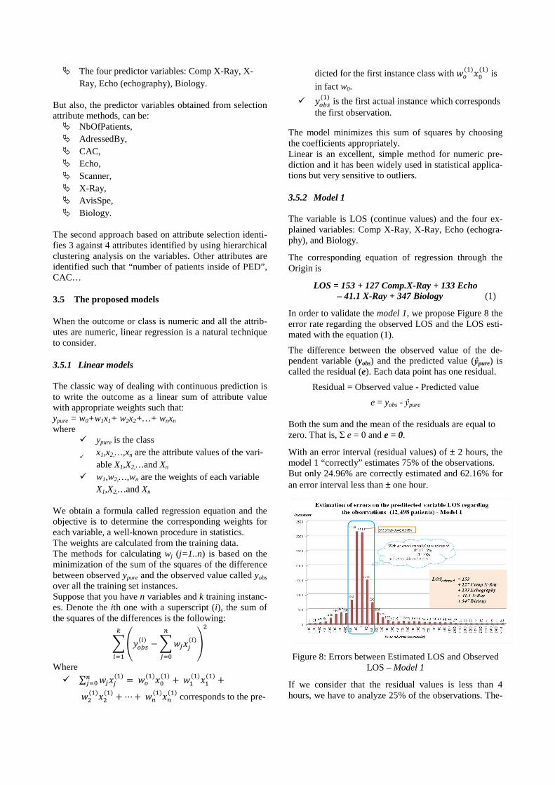
3.5.2 Model 1 The variable is LOS (continue values) and the four ex-plained variables: Comp X-Ray, X-Ray, Echo (echogra-phy), and Biology.

The corresponding equation of regression through the Origin is

LOS = 153 + 127 Comp.X-Ray + 133 Echo – 41.1 X-Ray + 347 Biology (1)

In order to validate the model 1, we propose Figure 8 the error rate regarding the observed LOS and the LOS esti-mated with the equation (1).

The difference between the observed value of the de-pendent variable (yobs) and the predicted value (ŷpure) is called the residual (e). Each data point has one residual.

Residual = Observed value - Predicted value

e = yobs - ŷpure

Both the sum and the mean of the residuals are equal to zero. That is, Σ e = 0 and e = 0.

With an error interval (residual values) of ± 2 hours, the model 1 “correctly” estimates 75% of the observations. But only 24.96% are correctly estimated and 62.16% for an error interval less than ± one hour.

Figure 8: Errors between Estimated LOS and Observed LOS – Model 1

If we consider that the residual values is less than 4 hours, we have to analyze 25% of the observations. The-

se Data points (called outliers) diverge in a big way from the overall pattern and we have to identify it. The main problem is that outlier greatly affects the slope of the regression line. It is absolutely necessary to test the influence of outliers; one way is to compute the re-gression equation without the outliers. 1) All the observations generating residual greater than

±180 minutes, 2) Analysis of all the observations considered outliers.

The regression equation through the Origin without outliers is:

LOS = 126 + 135 Comp.X-Ray + 91.6 Echo – 71.7 X-Ray + 323 Biology (2)

In this case, we guarantee that with a residual ±3h, we can found the duration of the 4 exams in minutes and we can estimate the LOS with an error of ± 3h. The sample is constituted of 9,719 patients (77.66% of the observed population). With respect to regression, outliers are influential only if they have a big effect on the regression equation. The difference between equation 1 and equation 2 shows that the substantial number of outliers has a relatively minor influence:

- 153-126, 27 minutes, - 127-137, -10 minutes, - 133-96.6, 36.4 minutes, - 41.1-71.7, -30.6 minutes, - 347-323, 24 minutes,

This is meaning that the model 1 overestimates at most than two hours compared to the model 2.

Sometimes, outliers do not have big effects when the data set is very large. It depends on the number of outiliers. The outliers represent 22.34% of the population but should be analyzed in order to try to identify patterns explaining the LOS.

3.5.3 Model 2 The target variable is LOS (continue values) and the eight predictor variables are:

� NbOfPatients � AdressedBy � CAC � Echo � Scanner � X-Ray � AvisSpe � Biology

LOS = - 2436 + 3.59 NbOfPatients + 17.8 AdressedBy + 0.816 CAC + 206 Echo + 171 Scanner + 75.2 X-Ray

+ 176 AvisSpe + 322 Biology (3)

Figure 8 presents the error rate regarding the observed LOS and the LOS estimated with the equation (3).

With a residual of ± 2 hours, the model 2 “correctly” estimates 73.76% of the observations. But only 28.24% are correctly estimated and 61.83% for an error interval less than ± one hour. For this model, the influence of outliers is not presented.

Figure 9: Errors between Estimated LOS and Observed LOS – Model 2

3.5.4 Discussion Two different models can predict the LOS. The first one is very easy to use for the medical staff. In fact it ex-plains the factor (corresponding to the variable) which increase or decrease the LOS. The meaning of the equation 1 (LOS = 153 + 127 Comp.X-Ray + 133 Echo – 41.1 X-Ray + 347 Biology) is the following regarding that the explained variables are Boolean:

If the patient does not need Comp.X-Ray, Echo, X-Ray and Biology, the LOS is around 153 minutes.

If the patient only needs Biology the LOS around 153 minutes increases of 347 minutes... The second model allows us to be more accurate in LOS estimation (28.24% regarding 24.96% for the model 1). But the use of the model 2 is more complex because it requires counting the number of people present in the PED for example, and requires taking into account more variables (8 against 4 for the model 1). The model 2 gives information such that the multiplica-tive factor of crowd whose value is 3.59 and corresponds to the weight of the variable NbOfPatients regarding LOS. We also observe that the weight of the variable Biology is quasi the same (323 for the model 1 without outliers and 322 for the model 2).

With the proposed approach, we illustrate that is possible to identify a very simple model. In this case, contrary to what is advocating in data mining, it is not always easy to discretize the variable target for classification and prediction.

Probably, these two models are dedicated to the PED of Lille’s Hospital, because the results are linked to the management of the hospital. It is not possible to general-ize to all the hospital Emergencies.

4 CONCLUSIONS AND FUTURE WORKS

We showed that different data mining techniques can be used beneficially in classification and prediction by using linear regression and we obtain a very “simple” model that it can easily use by the medical staff in order to estimate the LOS.

We experiment and validate the approach on real data concerning 12,498 patients. Data are collected from the database of the Pediatric Emergency unit located in France.

Given the presented care system and the methodological framework based on linear regression methods have been presented for LOS prediction. We identify two models. We retain the model 1 because it is very simple to under-stand and to use by the medical staff. We observe that the variable “number of patients inside of PED” deduced by using Monte-Carlo simulation does not have an important linear relationship with the LOS. Consequently, it is possible to estimate the LOS without taking into account “number of patients inside of PED” in the model 1. Only four variables allow us to explain LOS: The predictor variables are: Comp X-Ray, X-Ray, Echo (echography) and Biology. At the present time, we have to analyze the outliers representing approximately 25% of the observations for the model 1.

Of course, linear regression suffers from the disad-vantage of, well, linearity. Maybe the data exhibits a non-linear dependency, the best-fit straight line will be found, where “best” is interpreted as the least mean-square difference. So we analyze the interval error com-mitted with the obtained linear regression equation. In 75% of cases, we correctly fit with an error of ± 2 hours.

But the basic regression method is not able to discover nonlinear relationships between the others variables. Three issues are interesting to proceed in advancing this direction: a practical one, and two research issues. Firstly, it could be interesting to identify if there exist correlations but not necessary linear between the varia-bles. Secondly, we have to test the contribution of prob-abilistic view of the problem. Thirdly, we have to pro-pose a probabilistic model taking into account the non-linearity between variables.

References

Ahmad, A., Halawani, S.M., Albidewi, I.A., 2012. Novel ensemble methods for regression via classifica-tion problems. Expert Syst. Appl. 39, 6396–6401.

Austin, P.C., Tu, J.V., Lee, D.S., 2010. Logistic regres-sion had superior performance compared with regression trees for predicting in-hospital mor-tality in patients hospitalized with heart failure. J. Clin. Epidemiol. 63, 1145–1155.

Berg, M., 2001. Implementing information systems in health care organizations: myths and chal-lenges. Int. J. Med. Inf. 64, 143–156.

Chae, Y.M., Kim, H.S., Tark, K.C., Park, H.J., Ho, S.H., 2003. Analysis of healthcare quality indicator using data mining and decision support system. Expert Syst. Appl. 24, 167–172.

Dougherty, J., Kohavi, R., Sahami, M., 1995. Supervised and Unsupervised Discretization of Continuous Features. Presented at the Machine learning: proceedings of the twelfth international confe-rence, Morgan Kaufmann, pp. 194–202.

Duan, L., Street, W.N., Xu, E., 2011. Healthcare infor-mation systems: data mining methods in the creation of a clinical recommender system. En-terp. Inf. Syst. 5, 169–181.

Esfandiari, N., Babavalian, M.R., Moghadam, A.-M.E., Tabar, V.K., 2014. Knowledge discovery in medicine: Current issue and future trend. Expert Syst. Appl. 41, 4434–4463.

Filzmoser, P., 2008. Linear and nonlinear methods for regression and classification and applications in R. Institut f. Statistik u. Wahrscheinlichkeits-theorie 1040 Wien, Wiedner Hauptstr. 8-10/107 AUSTRIA http://www.statistik.tuwien.ac.at.

Hall, M., Frank, E., Holmes, G., Pfahringer, B., Reute-mann, P., Witten, I.H., 2009. The WEKA data mining software: an update. ACM SIGKDD Explor. Newsl. 11, 10.

Jain, A.K., Duin, R.P.W., Mao, J., 2000. Statistical pat-tern recognition: a review. IEEE Trans. Pattern Anal. Mach. Intell. 22, 4–37.

Kadri, F., Chaabane, S., Harrou, F., Tahon, C., 2014a. Modélisation et prévision des flux quotidiens des patients aux urgences hospitalières en utili-sant l’analyse de séries chronologiques, in: 7ème Conférence de Gestion et Ingénierie Des Systèmes Hospitaliers (GISEH), pp. 8.

Kadri, F., Chaabane, S., Harrou, F., Tahon, C., 2014b. Time series modelling and forecasting of emer-gency department overcrowding. J. Med. Syst., 38(9):107. doi: 10.1007/s10916-014-0107-0.

Kadri, F., Chaabane, S., Tahon, C., 2014c. A simulation-based decision support system to prevent and predict strain situations in emergency depart-ment systems. Simul. Model. Pract. Theory 42, 32–52.

Kadri, F., Pach, C., Chaabane, S., Berger, T., Trente-saux, D., Tahon, C., Sallez, Y., 2013. Modelling and management of the strain situations in hos-pital systems using un ORCA approach, IEEE IESM, 28-30 October. RABAT - MOROCCO, p. 10.

Kotsiantis, S.B., 2007. Supervised Machine Learning: A Review of Classification Techniques, in: Pro-ceedings of the 2007 Conference on Emerging Artificial Intelligence Applications in Computer Engineering: Real Word AI Systems with Ap-plications in eHealth, HCI, Information Retrie-val and Pervasive Technologies. IOS Press,

Amsterdam, The Netherlands, The Netherlands, pp. 3–24.

Kotsiantis, S.B., Zaharakis, I.D., Pintelas, P.E., 2006. Machine learning: a review of classification and combining techniques. Artif. Intell. Rev. 26, 159–190.

Kurt, I., Ture, M., Kurum, A.T., 2008. Comparing per-formances of logistic regression, classification and regression tree, and neural networks for predicting coronary artery disease. Expert Syst. Appl. 34, 366–374.

Landwehr, N., Hall, M., Frank, E., 2003. Logistic Model Trees, in: Lavrač, N., Gamberger, D., Blockeel, H., Todorovski, L. (Eds.), Machine Learning: ECML 2003, Lecture Notes in Computer Science. Springer Berlin Heidelberg, pp. 241–252.

Mazzocco, T., Hussain, A., 2012. Novel logistic regres-sion models to aid the diagnosis of dementia. Expert Syst. Appl. 39, 3356–3361.

Tan, P.., 2007. Introduction To Data Mining. Pearson Education.

Witten, I.H., Frank, E., Hall, M.A., more, & 0, 2011. Data Mining: Practical Machine Learning Tools and Techniques, Third Edition, 3 edition. ed. Morgan Kaufmann, Burlington, Mass.