correlation and regression measuring and predicting relationships

8/3/2019 Correlation and Regression Measuring and Predicting Relationships

http://slidepdf.com/reader/full/correlation-and-regression-measuring-and-predicting-relationships 1/25

Slide

11-1

2/10/2012

Chapter 11

Correlation and Regression:

Measuring and Predicting

Relationships



Slide

11-2

2/10/2012

Bivariate Data: Relationships

Examples of relationships:

Sales and earnings

Cost and number produced

Microsoft and the stock market

Effort and results

Scatterplot

± A picture to ex plore the relationship in bivariate data

Correlation r

± Measures strength of the relationship (from ±1 to 1)

Regression

± Predicting one variable from the other



Slide

11-3

2/10/2012

Interpreting Correlation

r = 1

± A perfect straight line

tilting up to the right

r = 0

± No overall tilt

± No relationship?

r = ± 1 ± A perfect straight line

tilting down to the right

X

Y

X

Y

X

Y

X

Y

X

Y

X

Y



Slide

11-4

2/10/2012

Example: Internet Site Ratings

Time Spent vs. Internet Pages Viewed

± Two measures of the abilities of 25 Internet sites

At the top right are eBay, Yahoo!, and MSN

± Correlation is r = 0.964

Very strong positive association (since r is close to 1)

± Linear relationship

Straight line

with scatter

± Increasing relationship Tilts up and to the right

Fig 11.1.3

0

30

60

90

0 100 200Pages per person

M i n u t e s

p e r p e r s o n

eBay

Yahoo!

MSN

0 100 200Pages per person

Yahoo!



Slide

11-5

2/10/2012

Example: Merger Deals

Dollars vs. Deals

± For mergers and acquisitions by investment bankers

244 deals worth $756 billion by Goldman Sachs

± Correlation is r = 0.419

Positive association


Straight line

with scatter

± Increasing relationship Tilts up and to the right

Fig 11.1.4

$0

$500

$1,000

0 100 200 300 400Deals

D o l l a r s ( b i l l i o n s )



Slide

11-6

2/10/2012

Example: Mortgage Rates & Fees

Interest Rate vs. Loan Fee

± For mortgages

If the interest rate is lower, does the bank make it up with a

higher loan fee?

± Correlation is r = ± 0.890 Strong negative association


Straight line

with scatter ± Decreasing relationship

Tilts down and to the right

Fig 11.1.5

5.0%

5.5%

6.0%

0% 1% 2% 3% 4%Loan fee

I n t e r

e s t r a t e



Slide

11-7

2/10/2012

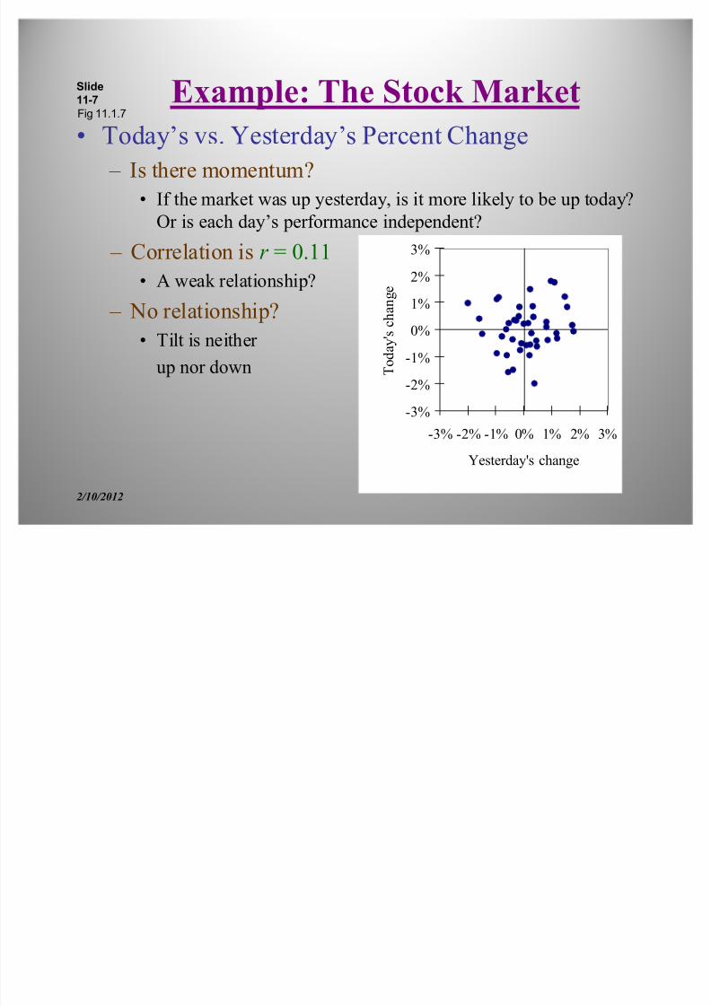
Example: The Stock Mark et

Today¶s vs. Yesterday¶s Percent Change

± Is there momentum?

If the market was up yesterday, is it more likely to be up today?

Or is each day¶s performance independent?

± Correlation is r = 0.11 A weak relationship?

± No relationship?

Tilt is neither

up nor down

Fig 11.1.7

-3%

-2%

-1%

0%

1%

2%

3%

-3% -2% -1% 0% 1% 2% 3%

Yesterday's change

T

o d a y ' s c h a n g e



Slide

11-8

2/10/2012

$0

$25

$50

$75

$100

$450 $500 $550 $600 $650

Strike Price

C a l l P r i c e

Call Price vs. Strike Price

± For stock options

³Call Price´ is the price of the option contract to buy stock at

the ³Strike Price´

The right to buy at a lower strike price has more value

± A nonlinear relationship

Not a straight line:

A curved relationship

± Correlation r =

± 0.895 A negative relationship:

Higher strike price goes

with lower call price

Example: Stock OptionsFig 11.1.10



Slide

11-9

2/10/2012

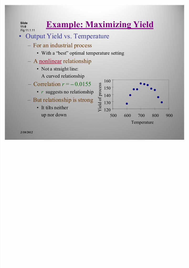
Example: Maximizing Yield

Output Yield vs. Temperature

± For an industrial process

With a ³best´ optimal temperature setting

± A nonlinear relationship

Not a straight line:

A curved relationship

± Correlation r = ± 0.0155

r suggests no relationship

± But relationship is strong It tilts neither

up nor down120

130

140

150

160

500 600 700 800 900

Temperature

Y i e l d o f p r o c e s s

Fig 11.1.11



Slide

11-10

2/10/2012

Example: Telecommunications

Circuit Miles vs. Investment (lower left)

± For telecommunications firms

± A relationship with unequal variability

More vertical variation at the right than at the left

Variability is stabilized by taking logarithms (lower right)

± Correlation r = 0.820

0

1,000

2,000

0 1,000 2,000Investment

($millions)

C i r c u i t m i l e s

( m i l l i o n

s )

15

20

15 20

Log of investment

L o g o f m i l e s

Fig 11.1.12,14

r = 0.957



Slide

11-11

2/10/2012

Example: Bond Coupon and Price

Price vs. Coupon Payment

± For trading in the bond market

Bonds paying a higher coupon generally cost more

± Two clusters are visible

Ordinary bonds (value is from coupon)

Inflation-indexed bonds (payout rises with inflation)


for all bonds

± Correlation r = 0.994 Ordinary bonds only

Fig 11.1.15

$100

$150

0% 5% 10%

B i d

p r i c e

0% 5% 10%Coupon rate



Slide

11-12

2/10/2012

Example: Cost and Quantity

Cost vs. Number Produced

± For a production facility

It usually costs more to produce more

± An outlier is visible

A disaster (a fire at the factory)

High cost, but few produced

3,000

4,000

5,000

20 30 40 50

Number produced

C o s t

0

10,000

0 20 40 60

Number produced

C o s t

Outlier removed:More details,

r = 0.869

r = ± 0.623

Fig 11.1.16,17



Slide

11-13

2/10/2012

Example: Salary and Experience

Salary vs. Years Ex perience

± For n = 6 employees

± Linear (straight line) relationship

± Increasing relationship

higher salary generally goes with higher ex perience


20

30

40

50

60

0 10 20 Ex perience S a l a r y ( $ t h o u s a n d )

Ex perience

15

1020

5

15

5

Salary

30

3555

22

40

27



Slide

11-14

2/10/2012

The Least-Squares Line Y =a+bX

Summarizes bivariate data: Predicts Y from X

± with smallest errors (in vertical direction, for Y axis)

± Intercept is 15.32 salary (at 0 years of ex perience)

± Slope is 1.673 salary (for each additional year of

ex perience, on average)

10

20

30

40

50

60

0 10 20Ex perience ( X )

S a l a

r y ( Y )



Slide

11-15

2/10/2012

Predicted Values and Residuals

Predicted Value comes from Least-Squares Line

± For example, Mary (with 20 years of ex perience)

has predicted salary 15.32+1.673(20) = 48.8

So does anyone with 20 years of ex perience

Residual is actual Y minus predicted Y

± Mary¶s residual is 55 ± 48.8 = 6.2

She earns about $6,200 more than the predicted salary for a

person with 20 years of ex perience

A person who earns less than predicted will have a negative

residual



Slide

11-16

2/10/2012

Predicted and Residual (continued)

10

20

30

40

50

60

0 10 20Ex perience

S a l a r y

Mary earns 55 thousand

Mary¶s predicted value is 48.8

Mary¶s residual is 6.2



Slide

11-17

2/10/2012

Standard Error of Estimate

Approximate size of prediction errors (residuals)

Actual Y minus predicted Y : Y ±[a+bX ]

Example (Salary vs. Ex perience)

Predicted salaries are about 6.52 (i.e., $6,520) away

from actual salaries

2

11

2

!

n

nr S S Y e

52.6

26

168667.01686.11

2 !

!

eS



Slide

11-18

2/10/2012

S e (continued)

Interpretation: similar to standard deviation

Can move Least-Squares Line up and down by S e ± About 68% of the data are within one ³standard error of

estimate´ of the least-squares line

(For a bivariate normal distribution)

20

30

40

50

60

0 10 20Ex perience

S a l a

r y



Slide

11-19

2/10/2012

Regression and Prediction Error

Predicting Y as Y (not using regression)

± Errors are approximately S Y = 11.686

Predicting Y as a+bX (using regression)

± E

rrors are approx

imately S e=

6.52 ± Errors are smaller when regression is used!

This is often the t rue payoff for using regression

Coefficient of Determination R2

± Tells what percent of the variability (variance) of Y isex plained by X

± Example: R2= 0.86672

= 0.751

Ex perience ex plains 75.1% of the variation in salaries



Slide

11-20

2/10/2012

Linear Model

Linear Model for the Population

± The foundation for statistical inference in regression

± Observed Y is a straight line, plus randomness

Y =

E+ F X +I

Randomness of individuals

Population relationship, on average {

X

Y

I



Slide

11-21

2/10/2012

Why Statistical Inf erence?

Because there can seem to be a relationship

± when, in fact, the population is just random

Samples of size n = 10

± from a po pul ation with no r el ationshi p (correlation 0) ± S am pl e correlations are not zero!

Due to the randomness of sampling

r = ± 0.471 r = 0.089 r = 0.395



Slide

11-22

2/10/2012

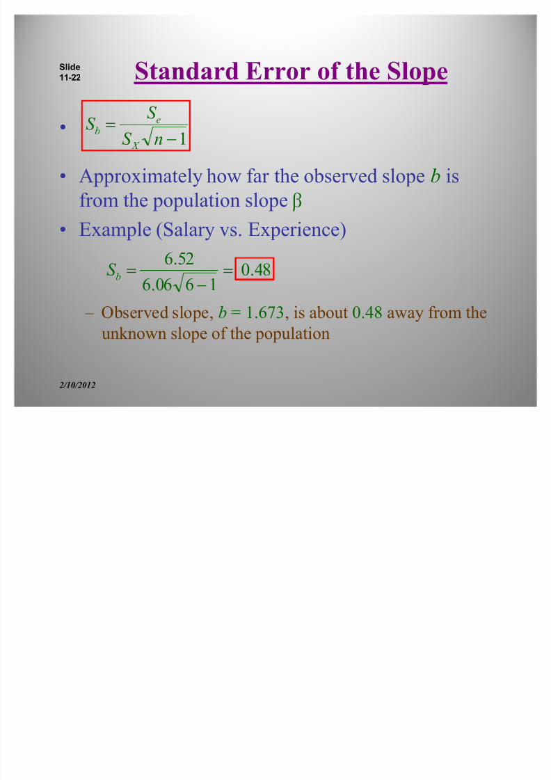
Standard Error of the Slope

Approximately how far the observed slope b is

from the population slope F

Example (Salary vs. Ex perience)

± Observed slope, b = 1.673, is about 0.48 away from the

unknown slope of the population

1!

nS

S S

X

eb

48.0

1606.6

52.6!

!bS



Slide

11-23

2/10/2012

Statistical Inf erence

Confidence Interval for the Slope

where t has n ± 2 degrees of freedom

Hypothesis Test Is F different from F0 = 0?

Is the regression significant?

Are X and Y significantly related?

± YES

If 0 is not in the confidence interval

± Or if |t st ati stic| = |b/S b| > t t able

± NO

Otherwise

bt S b s



Slide

11-24

2/10/2012

Example (Salary and Ex perience)

95% confidence interval for population slope F

use t = 2.776 from t table, 6 ± 2=4 degrees of freedom

± From 0.34 to 3.00 We are 95% sure that the po pul ation sl o pe is somewhere

between 0.34 and 3.00 ($thousand per year of ex perience)

Hypothesis test result

± S ignificant because 0 is not in the confidence interval

Ex per ience and S al ar y ar e significant l y r el ated

48.0776.2673.1 vs



Slide

11-25

2/10/2012

Regression Can Be Misleading

Linear Model May Be Wrong

± Nonlinear? Unequal variability? Clustering?

Predicting Intervention from Ex perience is Hard

± Relationship may become different if you intervene Intercept May Not Be Meaningful

± if there are no data near X = 0

Ex plaining Y from X vs. Ex plaining X from Y

± Use care in selecting the Y variable to be predicted

Is there a hidden ³Third Factor´?

± Use it to predict better with multiple regression?

correlation and regression measuring and predicting relationships

Documents