Xuhua Xia

Correlation and Regression

• Introduction to linear correlation and regression• Numerical illustrations• SAS and linear correlation/regression

– CORR

– REG

– GLM

• Assumptions of linear correlation/regression• Model II regression

Xuhua Xia

Introduction

• Correlation– Bivariate correlation

– Multiple correlation

– Partial correlation

– Canonical correlation

• Regression– Simple regression

– Multiple regression

– Nonlinear regression

(1857-1936)

(1822-1911)(1890-1962)

Xuhua Xia

Regression Coefficient

2

( )( ) 101

10( )

X X Y Yb

X X

, 2 2

( )( ) 101

10 10( ) ( )X Y

X X Y Yr

X X Y Y

2( )XSS X X 2( )YSS Y Y ( )( )XYS X X Y Y

3 1 3 0a Y bX

Y a bX X

1 1 4 4 4

2 2 1 1 1

3 3 0 0 0

4 4 1 1 1

5 5 4 4 4

Sum 15 15 10 10 10

X Y

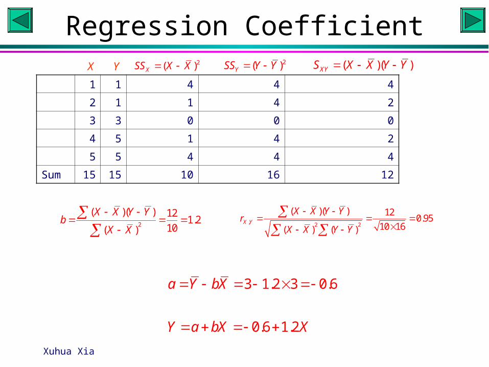
Change Y to 3, 4, 5, 6, 7 for students to recompute a and b.

Xuhua Xia

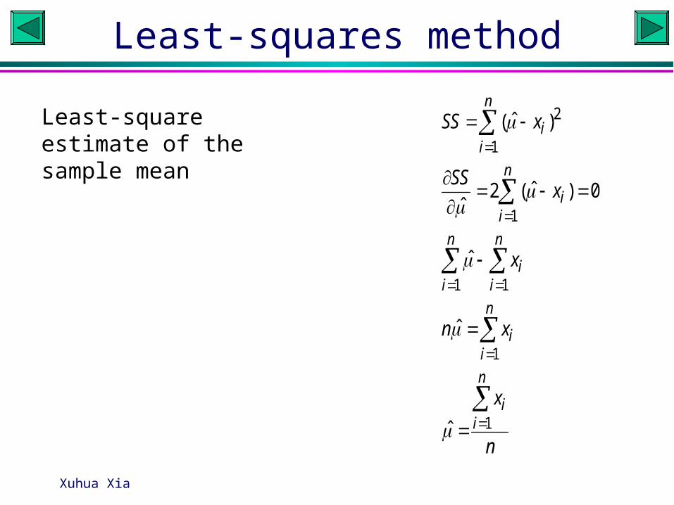
Least-squares method

2

1

1

1 1

1

1

ˆ( )

ˆ2 ( ) 0ˆ

ˆ

ˆ

ˆ

n

ii

n

ii

n n

ii i

n

ii

n

ii

SS x

SSx

x

n x

x

n

Least-square estimate of the sample mean

y x

ŷ a b x x

Q y y a b x x

Q

ay a b x x

Q

by a b x x x x

y a b x x

y a b x x x x

y a b x x

i i i

i i

i i i

i i

i i i

i i

i i i

i i

( )

( ) [ ( )]

[ ( )]

[ ( )]( )

[ ( )]

[ ( )]( )

( )

2 2

2 0

2 0

0

0

0

0

02

2

y n a ay

ny

y y b x x x x

y y x x b x x

by y x x

x x

ii

i i i

i i i

i i

i

;

[ ( )]( )

( )( ) ( )

( )( )

( )

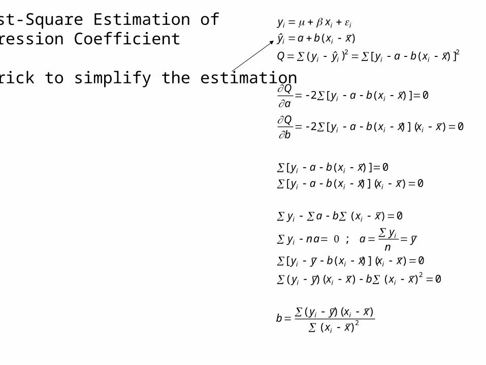
Least-Square Estimation ofRegression Coefficient

A trick to simplify the estimation

ŷi

Xuhua Xia

Maximum Likelihood Method

R. A. Fisher

Estimation of proportion of males (p) of a fish species in a pond:

Two samples are taken, one with 10 fish with 5 males and other with 12 fish but only 3 males

5 5 5 3 3 9 5 3 8 1410 12 10 12

5 310 12

(1 )

ln ln( ) 8ln 14ln(1 )

ln 8 140

1

8 5 3

22 10 12

L C p q C p q C C p p

L C C p p

L

p p p

p

Xuhua Xia

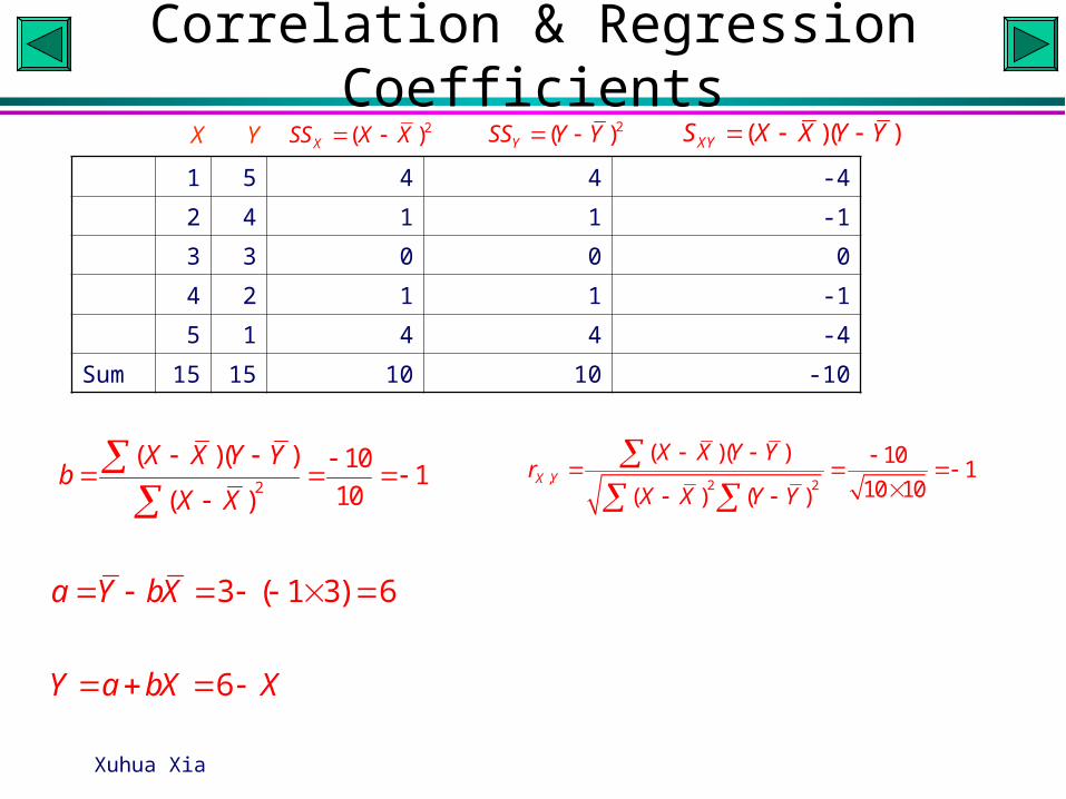
Correlation & Regression Coefficients

2

( )( ) 101

10( )

X X Y Yb

X X

, 2 2

( )( ) 101

10 10( ) ( )X Y

X X Y Yr

X X Y Y

3 ( 1 3) 6

6

a Y bX

Y a bX X

2( )XSS X X 2( )YSS Y Y ( )( )XYS X X Y Y

1 5 4 4 -4

2 4 1 1 -1

3 3 0 0 0

4 2 1 1 -1

5 1 4 4 -4

Sum 15 15 10 10 -10

X Y

Xuhua Xia

Regression Coefficient

2

( )( ) 121.2

10( )

X X Y Yb

X X

, 2 2

( )( ) 120.95

10 16( ) ( )X Y

X X Y Yr

X X Y Y

3 1.2 3 0.6

0.6 1.2

a Y bX

Y a bX X

2( )XSS X X 2( )YSS Y Y ( )( )XYS X X Y Y

1 1 4 4 4

2 1 1 4 2

3 3 0 0 0

4 5 1 4 2

5 5 4 4 4

Sum 15 15 10 16 12

X Y

Xuhua Xia

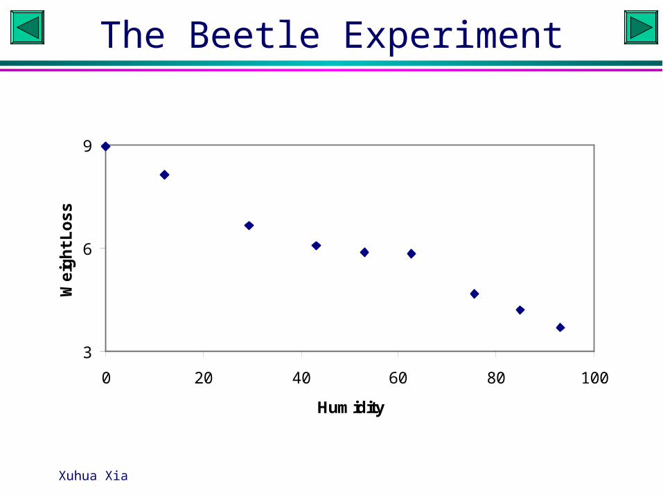
3

6

9

0 20 40 60 80 100

Humidity

We

igh

t L

os

sThe Beetle Experiment

Xuhua Xia

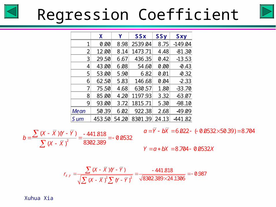
Regression Coefficient

2

( )( ) 441.8180.0532

8302.389( )

X X Y Yb

X X

, 2 2

( )( ) 441.8180.987

8302.389 24.1306( ) ( )X Y

X X Y Yr

X X Y Y

6.022 ( 0.0532 50.39) 8.704

8.704 0.0532

a Y bX

Y a bX X

X Y SSx SSy Sxy1 0.00 8.98 2539.04 8.75 -149.042 12.00 8.14 1473.71 4.48 -81.303 29.50 6.67 436.35 0.42 -13.534 43.00 6.08 54.60 0.00 -0.435 53.00 5.90 6.82 0.01 -0.326 62.50 5.83 146.68 0.04 -2.337 75.50 4.68 630.57 1.80 -33.708 85.00 4.20 1197.93 3.32 -63.079 93.00 3.72 1815.71 5.30 -98.10

Mean 50.39 6.02 922.38 2.68 -49.09Sum 453.50 54.20 8301.39 24.13 -441.82

Xuhua Xia

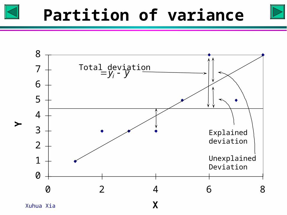
0

1

2

3

4

5

6

7

8

0 2 4 6 8

X

Y

Total deviation y yi

Explaineddeviation

Unexplained Deviation

Partition of variance

Xuhua Xia

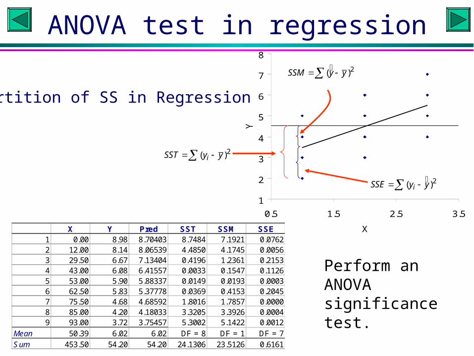
ANOVA test in regression

1

2

3

4

5

6

7

8

0.5 1.5 2.5 3.5

X

Y

2( )iSST y y

2( )SSM y y

2( )iSSE y y

X Y Pred SST SSM SSE1 0.00 8.98 8.70403 8.7484 7.1921 0.07622 12.00 8.14 8.06539 4.4850 4.1745 0.00563 29.50 6.67 7.13404 0.4196 1.2361 0.21534 43.00 6.08 6.41557 0.0033 0.1547 0.11265 53.00 5.90 5.88337 0.0149 0.0193 0.00036 62.50 5.83 5.37778 0.0369 0.4153 0.20457 75.50 4.68 4.68592 1.8016 1.7857 0.00008 85.00 4.20 4.18033 3.3205 3.3926 0.00049 93.00 3.72 3.75457 5.3002 5.1422 0.0012

Mean 50.39 6.02 6.02 DF = 8 DF = 1 DF = 7Sum 453.50 54.20 54.20 24.1306 23.5126 0.6161

Perform an ANOVA significance test.

Partition of SS in Regression

Xuhua Xia

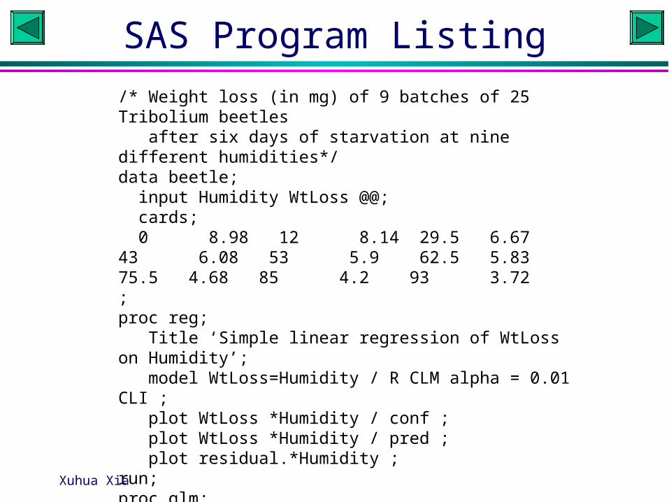
/* Weight loss (in mg) of 9 batches of 25 Tribolium beetles after six days of starvation at nine different humidities*/data beetle; input Humidity WtLoss @@; cards; 0 8.98 12 8.14 29.5 6.6743 6.08 53 5.9 62.5 5.8375.5 4.68 85 4.2 93 3.72;proc reg; Title ‘Simple linear regression of WtLoss on Humidity’; model WtLoss=Humidity / R CLM alpha = 0.01 CLI ; plot WtLoss *Humidity / conf ; plot WtLoss *Humidity / pred ; plot residual.*Humidity ;run;proc glm; model WtLoss=Humidity; Title ‘Simple linear regression of WtLoss on Humidity’;run;

SAS Program Listing

Xuhua Xia

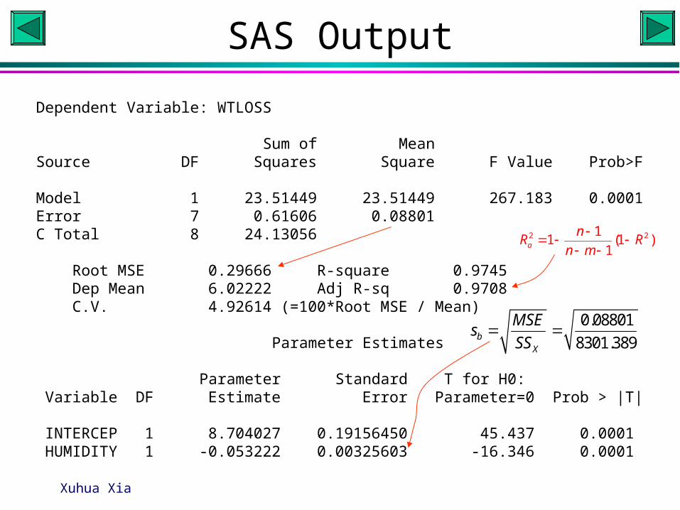
Dependent Variable: WTLOSS

Sum of MeanSource DF Squares Square F Value Prob>F

Model 1 23.51449 23.51449 267.183 0.0001Error 7 0.61606 0.08801C Total 8 24.13056

Root MSE 0.29666 R-square 0.9745 Dep Mean 6.02222 Adj R-sq 0.9708 C.V. 4.92614 (=100*Root MSE / Mean)

Parameter Estimates

Parameter Standard T for H0: Variable DF Estimate Error Parameter=0 Prob > |T|

INTERCEP 1 8.704027 0.19156450 45.437 0.0001 HUMIDITY 1 -0.053222 0.00325603 -16.346 0.0001

SAS Output

0.08801

8301.389bX

MSEs

SS

2 211 (1 )

1a

nR R

n m

Xuhua Xia

0

2

4

6

8

10

12

14

16

0 5 10 15

X

Y

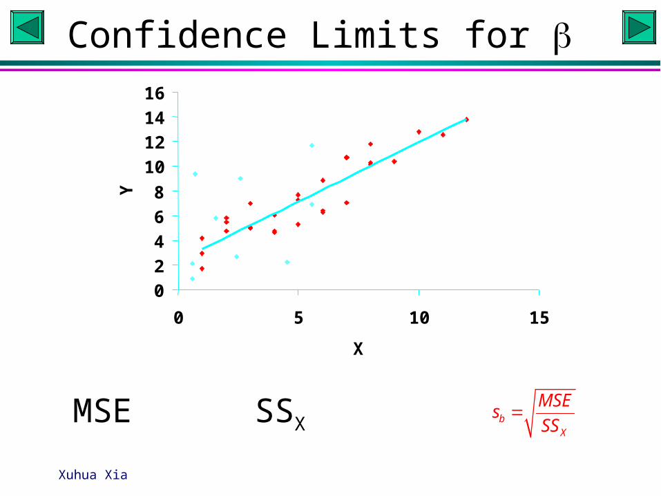
Confidence Limits for

bX

MSEs

SSMSE SSX

Xuhua Xia

0

2

4

6

8

10

12

14

16

0 5 10 15

X

Y

Confidence Limits for Y

2

ˆ

( )1i

iY

X

X Xs MSE

n SS

MSE SSXn Xi - Mean X

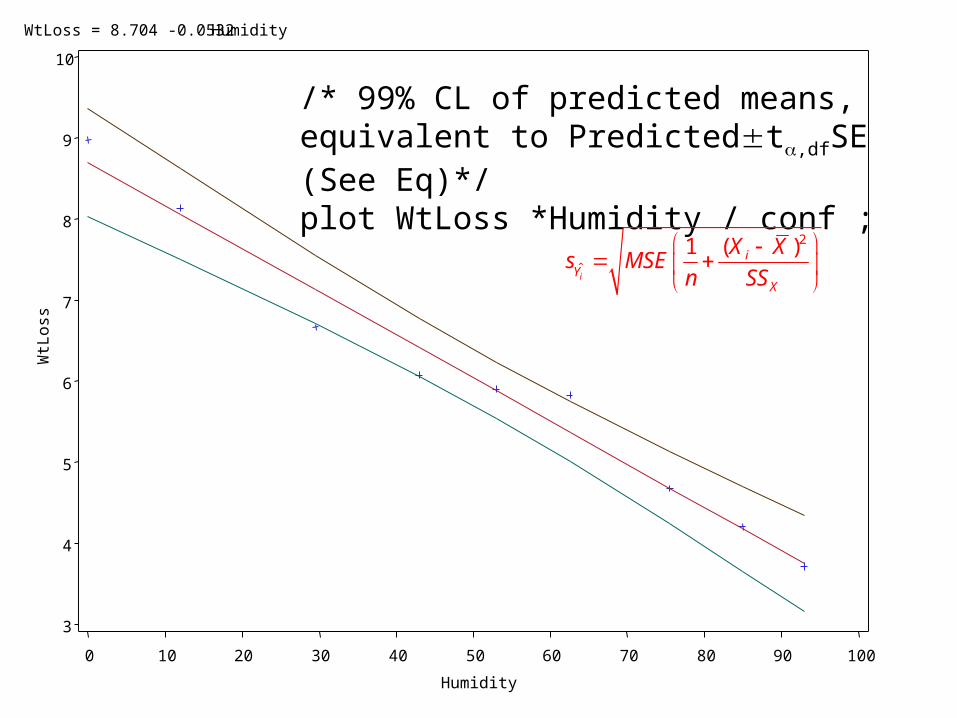
WtLoss = 8.704 -0.0532HumidityW

tLo

ss

3

4

5

6

7

8

9

10

Humidity

0 10 20 30 40 50 60 70 80 90 100

/* 99% CL of predicted means, equivalent to Predictedt,dfSE (See Eq)*/plot WtLoss *Humidity / conf ;

2

ˆ

( )1i

iY

X

X Xs MSE

n SS

WtL

oss

2

3

4

5

6

7

8

9

10

Humidity

0 10 20 30 40 50 60 70 80 90 100

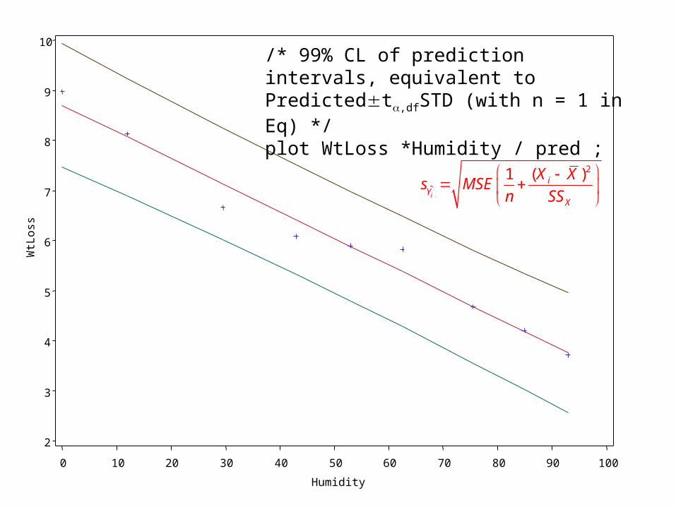
/* 99% CL of prediction intervals, equivalent to Predictedt,dfSTD (with n = 1 in Eq) */plot WtLoss *Humidity / pred ;

2

ˆ

( )1i

iY

X

X Xs MSE

n SS

Xuhua Xia

Regression summary

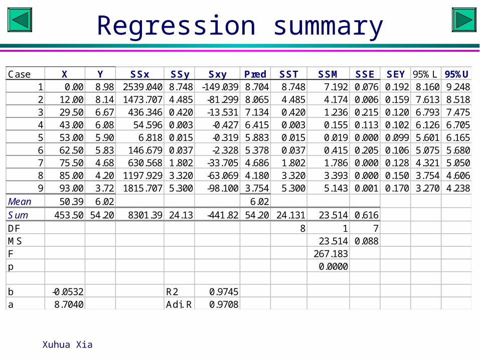
Case X Y SSx SSy Sxy Pred SST SSM SSE SEY 95%L 95%U1 0.00 8.98 2539.040 8.748 -149.039 8.704 8.748 7.192 0.076 0.192 8.160 9.2482 12.00 8.14 1473.707 4.485 -81.299 8.065 4.485 4.174 0.006 0.159 7.613 8.5183 29.50 6.67 436.346 0.420 -13.531 7.134 0.420 1.236 0.215 0.120 6.793 7.4754 43.00 6.08 54.596 0.003 -0.427 6.415 0.003 0.155 0.113 0.102 6.126 6.7055 53.00 5.90 6.818 0.015 -0.319 5.883 0.015 0.019 0.000 0.099 5.601 6.1656 62.50 5.83 146.679 0.037 -2.328 5.378 0.037 0.415 0.205 0.106 5.075 5.6807 75.50 4.68 630.568 1.802 -33.705 4.686 1.802 1.786 0.000 0.128 4.321 5.0508 85.00 4.20 1197.929 3.320 -63.069 4.180 3.320 3.393 0.000 0.150 3.754 4.6069 93.00 3.72 1815.707 5.300 -98.100 3.754 5.300 5.143 0.001 0.170 3.270 4.238

Mean 50.39 6.02 6.02Sum 453.50 54.20 8301.39 24.13 -441.82 54.20 24.131 23.514 0.616DF 8 1 7MS 23.514 0.088F 267.183p 0.0000

b -0.0532 R2 0.9745a 8.7040 Adj. R2 0.9708

Xuhua Xia

Assumptions

• The regression model Yi = + Xi + i

• Assumptions– The error term has a mean = 0, is independent and

normally distributed at each value of X, and have the same variance at each value of X (homoscedasticity).

– Y is linearly related to X

– There is negligible error (e.g., measurement error) for X. (Model II regression)

Xuhua Xia

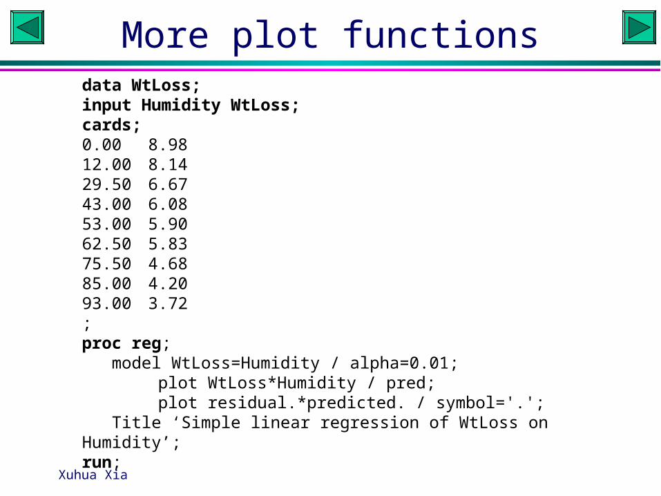
More plot functionsdata WtLoss;input Humidity WtLoss;cards;0.00 8.9812.00 8.1429.50 6.6743.00 6.0853.00 5.9062.50 5.8375.50 4.6885.00 4.2093.00 3.72;proc reg; model WtLoss=Humidity / alpha=0.01;

plot WtLoss*Humidity / pred; plot residual.*predicted. / symbol='.';

Title ‘Simple linear regression of WtLoss on Humidity’;run;

Xuhua Xia

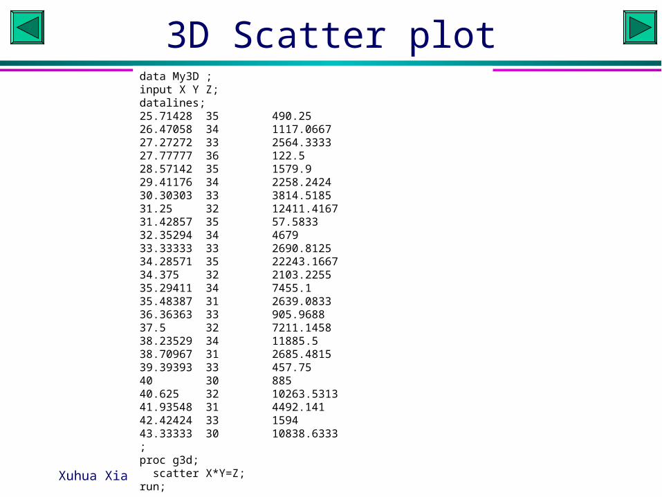
data My3D ;input X Y Z;datalines;25.71428 35 490.2526.47058 34 1117.066727.27272 33 2564.333327.77777 36 122.528.57142 35 1579.929.41176 34 2258.242430.30303 33 3814.518531.25 32 12411.416731.42857 35 57.583332.35294 34 467933.33333 33 2690.812534.28571 35 22243.166734.375 32 2103.225535.29411 34 7455.135.48387 31 2639.083336.36363 33 905.968837.5 32 7211.145838.23529 34 11885.538.70967 31 2685.481539.39393 33 457.7540 30 88540.625 32 10263.531341.93548 31 4492.14142.42424 33 159443.33333 30 10838.6333;proc g3d; scatter X*Y=Z;run;

3D Scatter plot

Xuhua Xia

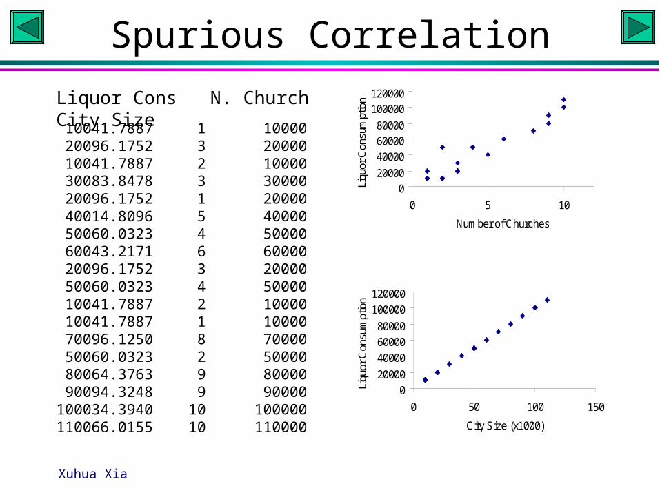
Spurious Correlation

10041.7887 1 1000020096.1752 3 2000010041.7887 2 1000030083.8478 3 3000020096.1752 1 2000040014.8096 5 4000050060.0323 4 5000060043.2171 6 6000020096.1752 3 2000050060.0323 4 5000010041.7887 2 1000010041.7887 1 1000070096.1250 8 7000050060.0323 2 5000080064.3763 9 8000090094.3248 9 90000

100034.3940 10 100000110066.0155 10 110000

Liquor Cons N. Church City Size

020000

40000

6000080000

100000120000

0 5 10

Number of Churches

Liqu

or C

onsu

mpt

ion

0

20000

40000

60000

80000

100000

120000

0 50 100 150

City Size (x1000)

Liqu

or C

onsu

mpt

ion

Xuhua Xia

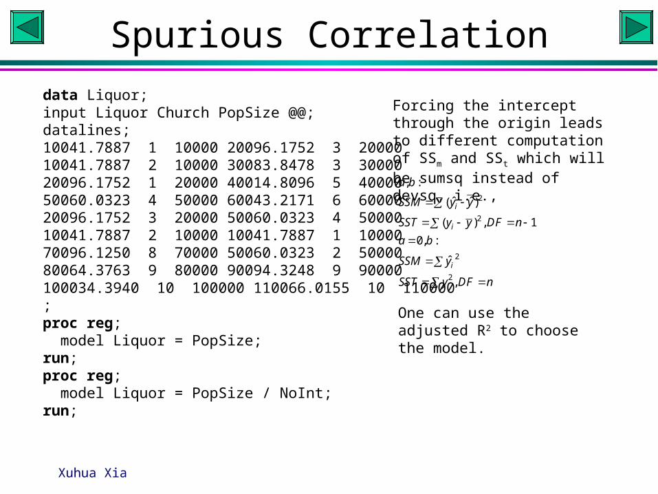
Spurious Correlation

data Liquor;input Liquor Church PopSize @@;datalines;10041.7887 1 10000 20096.1752 3 2000010041.7887 2 10000 30083.8478 3 3000020096.1752 1 20000 40014.8096 5 4000050060.0323 4 50000 60043.2171 6 6000020096.1752 3 20000 50060.0323 4 5000010041.7887 2 10000 10041.7887 1 1000070096.1250 8 70000 50060.0323 2 5000080064.3763 9 80000 90094.3248 9 90000100034.3940 10 100000 110066.0155 10 110000;proc reg; model Liquor = PopSize;run;proc reg; model Liquor = PopSize / NoInt;run;

Forcing the intercept through the origin leads to different computation of SSm and SSt which will be sumsq instead of devsq, i.e.,

2

2

2

2

, :

ˆ ˆ( )

( ) , 1

0, :

ˆ

,

i

i

i

a b

SSM y y

SST y y DF n

a b

SSM y

SST y DF n

One can use the adjusted R2 to choose the model.