performance evaluation of iscst3, adms-urban and …
TRANSCRIPT
S. Gulia et al., Int. J. Sus. Dev. Plann. Vol. 9, No. 6 (2014) 778–793
© 2014 WIT Press, www.witpress.comISSN: 1743-7601 (paper format), ISSN: 1743-761X (online), http://journals.witpress.comDOI: 10.2495/SDP-V9-N6-778-793
PERFORMANCE EVALUATION OF ISCST3, ADMS-URBAN AND AERMOD FOR URBAN AIR QUALITY MANAGEMENT IN
A MEGA CITY OF INDIA
S. GULIA1, S.M. SHIVA NAGENDRA2 & M. KHARE1
1Department of Civil Engineering, Indian Institute of Technology Delhi, New Delhi, India.2Department of Civil Engineering, Indian Institute of Technology Madras, Chennai, India.
ABSTRACTUrban air quality has deteriorated in last few decades in the mega cities of both developed and developing coun-tries. Many mathematical models have been widely used as prediction tool for urban air quality management in developed countries. However, applications of these models are limited in developing countries including India due to lack of suffi cient validation studies. In this paper, three state-of-the-art air quality models namely AERMOD, ADMS-Urban and ISCST3 have been used to predict the air quality at an intersection in Delhi city, India, followed by their performance evaluation and sensitive analysis under different meteorological condi-tions. The models have been run for different climatic conditions, i.e. summer and winter season to predict the concentration of carbon monoxide (CO), nitrogen dioxide (NO2) and PM2.5 (diameter size less than 2.5 µm). The ISCST3 has performed satisfactorily (d = 0.69) for predicting CO concentrations when compared with AERMOD (d = 0.50) and ADMS-Urban (d = 0.45) for winter period. The ADMS-Urban (d = 0.49) has per-formed satisfactorily for predicting NO2 concentration when compared with ISCST3 (d = 0.36) and AERMOD (d = 0.32). The AERMOD, ISCST3 and ADMS-Urban have performed satisfactorily for predicting PM2.5 con-centrations having d values as 0.46, 0.45 and 0.43 respectively. All three models have performed satisfactorily for predicting CO concentrations when wind speed was in the range of 0.5–3 m/s and wind direction in the range 90–180 degrees, i.e. downwind direction. The difference in model’s performance may be due to differ-ences in model formulation and the treatment of terrain features. The causal nature of these Gaussian based models may be one of the reasons for difference in performance of the models, because these are sensitive to quality and quantity of input data on meteorology and emission sources.Keywords: AERMOD, ADMS-Urban, ISCST3, input data, model evaluation, urban air quality management.
1 INTRODUCTIONUrban air quality in majority of the megacities in the world is getting deteriorated due to increasing industrialization and urbanization [1,2]. In developed countries, trends of urbanization and associated growth of cities have started to reverse due to severe levels of congestion [3]. However, in the develop-ing countries, the city’s growth is from periphery to core. Like many cities in the developed country, Indian cities are also growing at a faster rate. The motorized transport is the principle source of local urban air pollution in mega cities of developing countries because of the increased vehicular popula-tion, vehicle kilometre travelled (VKT) and lack of infrastructure development [4]. In Indian metropolitan cities, the vehicles are estimated to account for 70% of CO, 50% of HC, 30–40% of NOx, 30% of SPM and 10% of SO2 of the total air pollution load of these cities, of which two-third is con-tributed by two wheelers alone [5]. This rapid growth of motor vehicles ownership and activities in Indian cities are causing a wide range of serious health, environmental and socio-economic impacts [6]. The total motor vehicles’ population in India has also increased from 0.3 million in 1951 to 115 million in year 2009 of which, two wheelers account for 70% of the total vehicular population [7].
The success of urban air quality management plan (UAQMP) mainly depends upon the system-atic networking between its components, i.e. air quality goals, monitoring network system, air quality prediction and forecasting tools, emission control strategies, emergency alert system, public
S. Gulia et al., Int. J. Sus. Dev. Plann. Vol. 9, No. 6 (2014) 779
information system, policy implementation and evaluation. The air quality prediction and forecast-ing by air quality models plays an important role in formulating air pollution control and management strategies on ‘What If’ scenarios [8]. Air quality modelling provides the ability to assess the current and future air quality in order to enable (informed) policy decisions to be made [9]. The planning and implementation of urban air quality management practices in developing countries is a challenging task for policy makers. The major challenges are lack of government commitment and stakeholder participation, weaknesses in policies, standards and regulations, defi -ciencies in real-time air quality monitoring, lack of data management, limited scope of air quality modelling, emission inventories often absent, incomplete or inaccurate [10]. Many mathematically models have been widely used for urban air quality management in developed world [9]. However, their applications are limited in developing countries like India due to lack of readily available input data, time and cost involved in collecting the required model input data [4]. Line source dis-persion models represent essential computational tools for predicting the air quality impacts of emissions from road traffi c and are widely used in city level air quality planning [9]. They are extensively used throughout the world including India to carry out the prediction of vehicular pol-lutant concentrations along highways in both urban as well rural areas. Majumdar et al., [11] reveal that CALINE 4 with correction factors (0.37) can be applied reasonably well for the prediction of CO in the city of Kolkata. Bhanarkar et al. [12] assessed the SO2 and NO2 pollution level in Jam-shedpur region using ISCST3 model and observed that the predicted 24-h concentrations have good agreement with measured concentrations at 11 ambient air monitoring stations. The commercially available air quality models, e.g. AERMOD [13] and ADMS-Urban [14], are highly advanced and complex but user-friendly. They are performing satisfactorily with old generation line source dis-persion models such as CALINE 4, GFLSM and DFLSM [15]. Kumar et al., [16] observed that AERMOD has a tendency to under-predict both under stable and unstable conditions when the model was applied for Ohio, USA. Long et al., [17] studied that sensitivity of AERMOD to input parameters and found out that AERMOD is very sensitive to surface roughness than other input parameters like solar radiation, cloud cover and albedo. Faulkner et al., [18] observed that the ISCST3 is sensitive to changes in wind speed, temperature, solar radiation (as it affects stability class), and mixing heights below 160 m. Further, surface roughness also affected downwind con-centrations predicted by ISCST3. They also noticed that AERMOD was sensitive to changes in albedo, surface roughness, wind speed, temperature, and cloud cover. Over 70 U.K. local authori-ties [19] have extensively used the ADMS-Urban for control of air pollution at designated air quality control regions (AQCRs). In India, the application of AERMOD and ADMS-Urban models for urban air quality assessment are limited. Mohan et al., [20] found out that AERMOD has a greater tendency to over-predict when compared to ADMS-Urban. They observed that this is due to difference in treatment of atmospheric stability. The performance and accuracy of the air quality models mainly depends upon accuracy input parameters. The ISCST3 model works on the Pas-quill-Gifford stability class while AERMOD and ADMS-Urban worked on the Monin-Abukhov length. AERMOD required upper air sounding meteorological data. In this study, three state-of-the-art air quality models, i.e. ISCST3, ADMS-Urban and AERMOD have been set up and run to predict air pollutants’ concentrations at Income Tax Offi ce (ITO), intersection in Delhi city, India, followed by their performance evaluation in different meteorological condition.
2 MODELS’ DESCRIPTIONAERMOD is a replacement of the ISCST3 model which incorporates the effects on dispersion from vertical variations in the planetary boundary layer (PBL). The plume growth is determined by turbu-lence profi les that vary with height. AERMOD calculates the convective and mechanical mixing
780 S. Gulia et al., Int. J. Sus. Dev. Plann. Vol. 9, No. 6 (2014)
height. It includes the concept of dividing streamlines and the fl ume is modelled as combinations of terrain – following and terrain impacting states [13,21]. It consists of two pre-processors, i.e. AER-MET (meteorological pre-processor) and AERMAP (terrain pre-processors). Input data for AERMET includes hourly cloud cover observations, surface meteorological observations such as wind speed and direction, temperature, dew point, humidity and sea level pressure and twice-a-day upper air soundings. The AERMAP uses gridded terrain data (digital elevations model data) to cal-culate a representative terrain-infl uence height (hc). It is uniquely defi ned for each receptor location and is used to calculate the dividing streamline height.
The ADMS-Urban has been developed by Cambridge Environmental Research Consultants Ltd. UK. It is an advanced model for predicting concentrations of pollutants emitted both continuously from point, line, volume and area sources, and discretely from point sources. The model incorpo-rates parameterization of boundary layer based on Monin-Obhukov length and boundary layer height. In this model also, non-Gaussian vertical profi le of concentration is created in convective conditions, which allows for the skewed nature of turbulence within the atmospheric boundary layer that can lead to high surface concentrations near the source [18,22].
The ISCST3 model is a steady-state Gaussian plume air dispersion model [23]. It is capable of estimating pollutant concentration from point, line and area sources. It uses Brigg’s equations with stack top wind speed and vertical temperature gradient. The boundary layer parameters are mixing heights, P-G stability class and surface roughness length.
The check list of input data required by each model is given in Table 1.
3 MATERIALS AND METHODS
3.1 Site characteristics
The Income Tax Offi ce (ITO) is one of the busiest intersections in Delhi and located at 28°37’39.70” N and 77014’28.60” E. The four major roads meet at this intersection. The ITO intersection is sur-rounded by both commercial and residential area. The pollution monitoring site governed by CPCB is located 12 m from BSZ Marg outside the premises of Indian National Science Academy (INSA) (Fig. 1).
The air quality of ITO intersection has been degraded due to heavy traffi c load most probably during peak hours. Mohan and Kandya [24] has calculated AQI for Delhi city based on 9 years’ pol-lution monitoring data at seven different locations and found that air quality at ITO intersection is worst in the city amongst all monitoring stations, which may be due to high traffi c density and con-gestion at the ITO intersection. The annual average concentration of CO and PM2.5 at BSZ marg was 2469 and 102 µg/m3, respectively, during 2007, while monthly average concentration of CO and PM2.5 varied from 1688 to 4531 µg/m3 and 34 to 198 µg/m3, respectively. High levels of CO and PM2.5 concentration might be attributed to the increase in vehicular population in Delhi [25]. Goyal et al. [26] reported that 17% and 28% of total NOx and PM concentration respectively are due to vehicular pollution, which is almost the same as those from other sources such as industry, power plants and domestic uses in Delhi.
3.2 Traffi c characteristic
The traffi c data at ITO intersection has been collected from Central Road Research Institute (CRRI), New Delhi. The traffi c volume on road 3 and 4 has been observed to be greater than other two roads (road 1 and 2).

S. Gulia et al., Int. J. Sus. Dev. Plann. Vol. 9, No. 6 (2014) 781
Table 1: Check list of input data requirement for all three models.
Parameters AERMOD ADMS-Urban ISCST3
Site information (latitude, longitude, base elevation, time zone (GMT).
√ √ √
Source type √ √ √Met data Year, month, day, hour √ √ √Cloud cover (tenths) √ √* √Temperature (°c) √ √ √Relative humidity (%) √ Optional √Pressure (mbar) √ Optional √Wind direction (degrees) (north as 360 degree) √ √ √Wind speed (m/s) √ √** √Ceiling height (m) √ √Hourly precipitation (inches) √ Optional √ Global horizontal radiation (Wh/m2) √ Optional √Upper air data for AERMET (NCDC-TD 6201 variable length) – pressure (Pa), height (m), tem-perature (°C), relative humidity (%), wind direc-tion (degree), wind speed (m/s)
√ Optional
Albedo √Bowen ratio √
Surface roughness length (m) √ √ √Site map (.shp fi le) and DEM formatted terrain data (xt, yt, zt)
√ √ √
Monin-Obhukov length (m) OptionalMixing height (m) √Stability class √Emission rates (g/s) for each types of pollutant √ √ √Height of the source (m) √ √ √Background concentration of pollutants √ √ √
*Unit of cloud cover is Oktas.**Minimum threshold wind speed is 0.75 m/s.
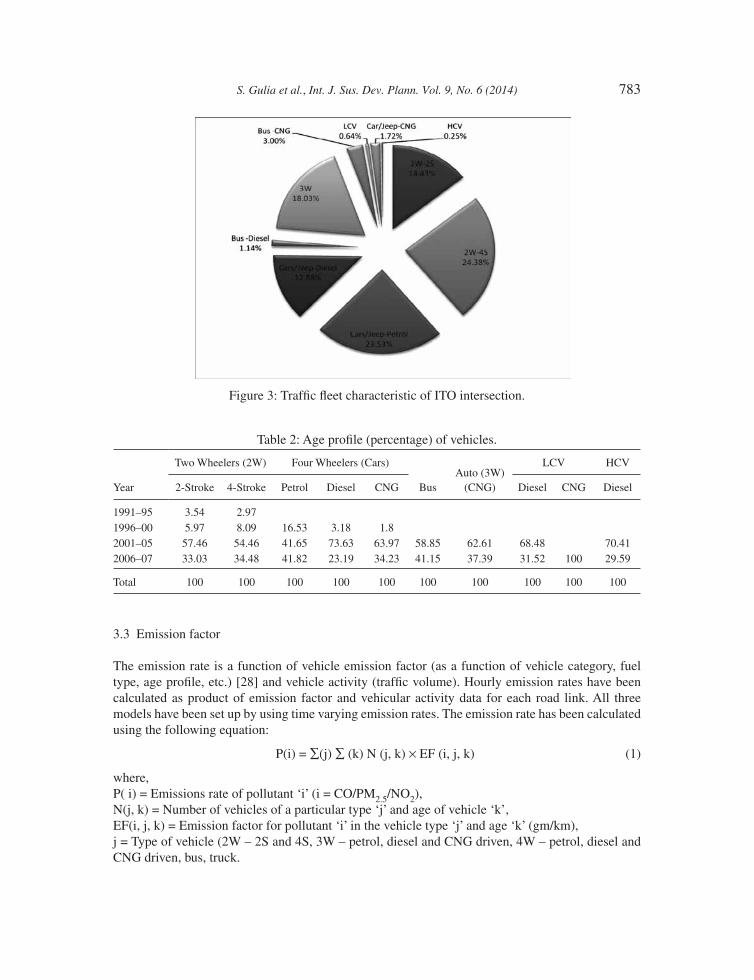
Maximum traffi c has been observed between 8:00 and 10:00 am (morning peak hour) and between 5:00 and 7:00 pm (evening peak hours) (Fig. 2). The traffi c fl eet of Delhi is composed of two wheeler (2-stroke and 4-stroke), three wheeler (CNG driven), cars/jeep (petrol, diesel and Compressed Natural Gas, CNG driven), light commercial vehicle (LCV), buses (CNG and diesel driven) and heavy commercial vehicle (HCV). The traffi c fl eet of ITO intersection is shown in Fig. 3.
The portion of two wheeler (2W) is highest, i.e. 38.8% (2W-2-stroke = 14.4% and 2W-4-stroke = 24.4%) followed by cars 36.3% (petrol driven = 23.5% and diesel driven = 12.8%). In total traffi c

782 S. Gulia et al., Int. J. Sus. Dev. Plann. Vol. 9, No. 6 (2014)
Figure 2: Diurnal traffi c pattern at the ITO intersection.
composition, the three wheeler (CNG driven) is 18.0% and bus is 4.1% (CNG driven = 3% and diesel driven = 1.1%). Age of the vehicle can affect the emission characteristic of the exhaust. An old and poorly maintained vehicle generates more emission compared to new vehicle. The assessment of vintage profi les of local traffi c is very diffi cult job especially when traffi c characteristics are het-erogeneous in nature. The vintage profi le data of traffi c was collected by fuel station survey at different petrol pumps and CNG fi lling stations along the road corridor. This included fi nding out percentage of two stroke (2S) and four stroke (4S) vehicles in two wheeler and percentage of petrol and diesel and CNG driven vehicles in four wheeler (i.e. car categories). It has been further assumed that the vehicles plying on the road, could be represented by vehicles (in terms of their age profi le, engine technology and composition) captured during the fuel station survey [27]. The vintage profi le of the vehicles of Delhi is given in Table 2.
Figure 1: Site view of ITO intersection, Delhi.
S. Gulia et al., Int. J. Sus. Dev. Plann. Vol. 9, No. 6 (2014) 783
3.3 Emission factor
The emission rate is a function of vehicle emission factor (as a function of vehicle category, fuel type, age profi le, etc.) [28] and vehicle activity (traffi c volume). Hourly emission rates have been calculated as product of emission factor and vehicular activity data for each road link. All three models have been set up by using time varying emission rates. The emission rate has been calculated using the following equation:
P(i) = ∑(j) ∑ (k) N (j, k) × EF (i, j, k) (1)
where,P( i) = Emissions rate of pollutant ‘i’ (i = CO/PM2.5/NO2), N(j, k) = Number of vehicles of a particular type ‘j’ and age of vehicle ‘k’,EF(i, j, k) = Emission factor for pollutant ‘i’ in the vehicle type ‘j’ and age ‘k’ (gm/km),j = Type of vehicle (2W – 2S and 4S, 3W – petrol, diesel and CNG driven, 4W – petrol, diesel and CNG driven, bus, truck.
Figure 3: Traffi c fl eet characteristic of ITO intersection.
Table 2: Age profi le (percentage) of vehicles.
Year
Two Wheelers (2W) Four Wheelers (Cars)
BusAuto (3W)
(CNG)
LCV HCV
2-Stroke 4-Stroke Petrol Diesel CNG Diesel CNG Diesel
1991–95 3.54 2.971996–00 5.97 8.09 16.53 3.18 1.82001–05 57.46 54.46 41.65 73.63 63.97 58.85 62.61 68.48 70.412006–07 33.03 34.48 41.82 23.19 34.23 41.15 37.39 31.52 100 29.59
Total 100 100 100 100 100 100 100 100 100 100
784 S. Gulia et al., Int. J. Sus. Dev. Plann. Vol. 9, No. 6 (2014)
3.4 Meteorological data
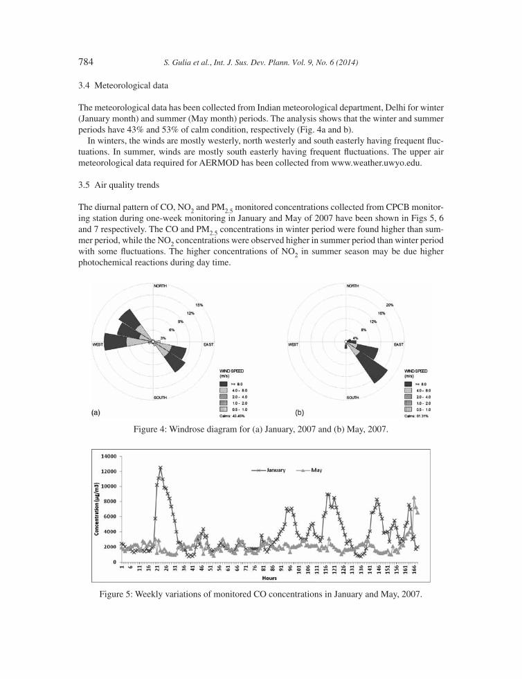
The meteorological data has been collected from Indian meteorological department, Delhi for winter (January month) and summer (May month) periods. The analysis shows that the winter and summer periods have 43% and 53% of calm condition, respectively (Fig. 4a and b).
In winters, the winds are mostly westerly, north westerly and south easterly having frequent fl uc-tuations. In summer, winds are mostly south easterly having frequent fl uctuations. The upper air meteorological data required for AERMOD has been collected from www.weather.uwyo.edu.
3.5 Air quality trends
The diurnal pattern of CO, NO2 and PM2.5 monitored concentrations collected from CPCB monitor-ing station during one-week monitoring in January and May of 2007 have been shown in Figs 5, 6 and 7 respectively. The CO and PM2.5 concentrations in winter period were found higher than sum-mer period, while the NO2 concentrations were observed higher in summer period than winter period with some fl uctuations. The higher concentrations of NO2 in summer season may be due higher photochemical reactions during day time.
Figure 4: Windrose diagram for (a) January, 2007 and (b) May, 2007.
Figure 5: Weekly variations of monitored CO concentrations in January and May, 2007.

S. Gulia et al., Int. J. Sus. Dev. Plann. Vol. 9, No. 6 (2014) 785
The background concentrations for CO for the months of January and May have been 1400 and 1250 µg/m3, respectively. The background concentrations for NO2 and PM2.5 have been taken cor-responding to the lowest point on the curve of monitored data [29]. The background concentrations of NO2 for winter and summer period have been taken as 61 µg/m3 and 40 µg/m3, respectively. The background concentration of PM2.5 for winter and summer season has been taken as 83 µg/m3 and 25 µg/m3, respectively.
4 RESULTS AND DISCUSSIONSAll three models have been set up for the prediction of CO, NO2 and PM2.5 concentrations for winter as well as summer period. The whole intersection has been divided in ten road links based on traffi c count and road alignment. All three models have been run for fl at terrain. The hourly monitored pol-lutants’ concentrations have been compared with the predicted concentrations by measuring some statistical parameters, which have been used in earlier studies related to model validation [16,20]. Statistical descriptors, mainly index of agreement ‘d’, factor of 2 (FAC2), fractional bias (FB) and normal mean square error (NMSE), have been used to evaluate the model performance. According to Kumar et al., [16] the performance of the model can be deemed acceptable if: 0.4 ≤ d ≤ 1.0, −0.5 ≤ NMSE ≤ 0.5, 0.5 ≤ FB ≤ 0.5 and FAC2 ≥ 0.8. Tables 3, 4 and 5 show the model performance results in both winter and summer season.
Figure 6: Weekly variations of monitored NO2 concentrations for January and May, 2007.
Figure 7: Weekly variations of monitored PM2.5 concentrations for January and May, 2007.
786 S. Gulia et al., Int. J. Sus. Dev. Plann. Vol. 9, No. 6 (2014)
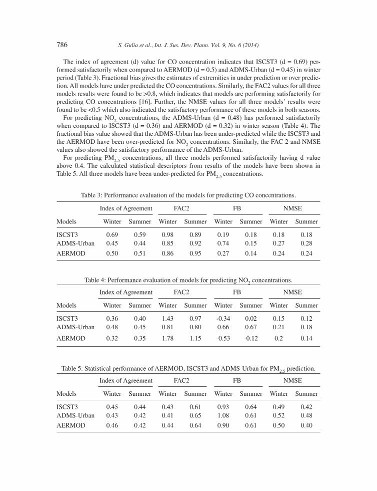
The index of agreement (d) value for CO concentration indicates that ISCST3 (d = 0.69) per-formed satisfactorily when compared to AERMOD (d = 0.5) and ADMS-Urban (d = 0.45) in winter period (Table 3). Fractional bias gives the estimates of extremities in under prediction or over predic-tion. All models have under predicted the CO concentrations. Similarly, the FAC2 values for all three models results were found to be >0.8, which indicates that models are performing satisfactorily for predicting CO concentrations [16]. Further, the NMSE values for all three models’ results were found to be <0.5 which also indicated the satisfactory performance of these models in both seasons.
For predicting NO2 concentrations, the ADMS-Urban (d = 0.48) has performed satisfactorily when compared to ISCST3 (d = 0.36) and AERMOD (d = 0.32) in winter season (Table 4). The fractional bias value showed that the ADMS-Urban has been under-predicted while the ISCST3 and the AERMOD have been over-predicted for NO2 concentrations. Similarly, the FAC 2 and NMSE values also showed the satisfactory performance of the ADMS-Urban.
For predicting PM2.5 concentrations, all three models performed satisfactorily having d value above 0.4. The calculated statistical descriptors from results of the models have been shown in Table 5. All three models have been under-predicted for PM2.5 concentrations.
Table 3: Performance evaluation of the models for predicting CO concentrations.
Models
Index of Agreement FAC2 FB NMSE
Winter Summer Winter Summer Winter Summer Winter Summer
ISCST3 0.69 0.59 0.98 0.89 0.19 0.18 0.18 0.18ADMS-Urban 0.45 0.44 0.85 0.92 0.74 0.15 0.27 0.28
AERMOD 0.50 0.51 0.86 0.95 0.27 0.14 0.24 0.24
Table 4: Performance evaluation of models for predicting NO2 concentrations.
Models
Index of Agreement FAC2 FB NMSE
Winter Summer Winter Summer Winter Summer Winter Summer
ISCST3 0.36 0.40 1.43 0.97 -0.34 0.02 0.15 0.12ADMS-Urban 0.48 0.45 0.81 0.80 0.66 0.67 0.21 0.18
AERMOD 0.32 0.35 1.78 1.15 -0.53 -0.12 0.2 0.14
Table 5: Statistical performance of AERMOD, ISCST3 and ADMS-Urban for PM2.5 prediction.
Models
Index of Agreement FAC2 FB NMSE
Winter Summer Winter Summer Winter Summer Winter Summer
ISCST3 0.45 0.44 0.43 0.61 0.93 0.64 0.49 0.42ADMS-Urban 0.43 0.42 0.41 0.65 1.08 0.61 0.52 0.48
AERMOD 0.46 0.42 0.44 0.64 0.90 0.61 0.50 0.40
S. Gulia et al., Int. J. Sus. Dev. Plann. Vol. 9, No. 6 (2014) 787
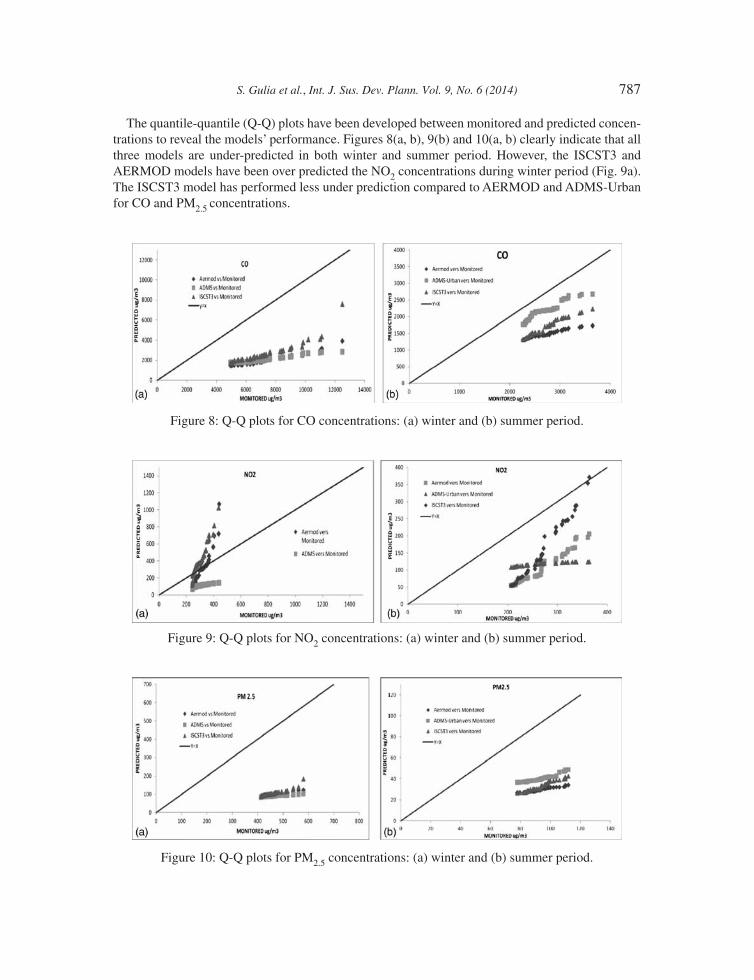
The quantile-quantile (Q-Q) plots have been developed between monitored and predicted concen-trations to reveal the models’ performance. Figures 8(a, b), 9(b) and 10(a, b) clearly indicate that all three models are under-predicted in both winter and summer period. However, the ISCST3 and AERMOD models have been over predicted the NO2 concentrations during winter period (Fig. 9a). The ISCST3 model has performed less under prediction compared to AERMOD and ADMS-Urban for CO and PM2.5 concentrations.
Figure 8: Q-Q plots for CO concentrations: (a) winter and (b) summer period.
Figure 9: Q-Q plots for NO2 concentrations: (a) winter and (b) summer period.
Figure 10: Q-Q plots for PM2.5 concentrations: (a) winter and (b) summer period.

788 S. Gulia et al., Int. J. Sus. Dev. Plann. Vol. 9, No. 6 (2014)
4.1 Models’ sensitivity
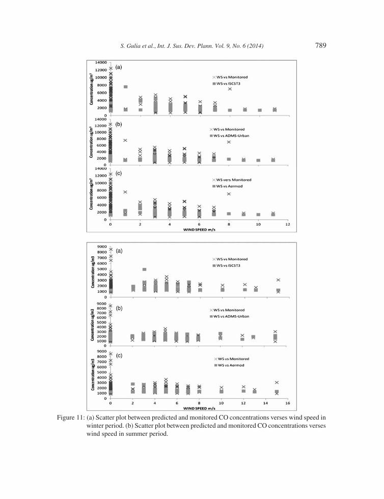
The models’ sensitivity analysis has been carried out for CO concentrations with respect to wind speed and direction. The ‘d’ value (Table 6) indicates that ISCST3 and AERMOD models have performed unsatisfactorily under calm wind condition because they failed to consider ‘lag effect’, in which CO accumulates due to worse meteorological conditions (inversions) sup-pressing the dispersion [9]. The ADMS-Urban can predict satisfactorily when compared to AERMOD and ISCST3 in calm meteorological condition, because it consider the wind speed of 0.75 m/s as threshold. All three models have performed satisfactorily when wind speed was in the range of 0.5–3 m/s. The ISCST3 model performed satisfactorily (d = 0.84) in wind speed range of 0.5–3 m/s when compared to AERMOD (d = 0.53) and ADMS-Urban (d = 0.45) in winter period.
Similarly, the scatter plot (Fig. 11a and b) indicated the performance of models for predict-ing CO concentrations with different wind speed range in winter and summer seasons, respectively.
The sensitivity of the models’ predictions for different wind direction have been analysed by cat-egorizing the wind direction into the ranges of 90–180, 180–270 and 270–360 degree. The wind direction between 360 (as North) and 90 degrees was negligible during the study period (Fig. 4a and b). The ‘d’ value (Table 7) indicates that all three models have predicted CO concentrations satisfactorily when wind direction was in range of 90–180 degrees. The satisfactory performance of models in this direction might be due to heavy traffi c volume on road 3 and road 4 in the same direc-tion (Fig. 1), i.e. receptor location is in downwind direction. The AERMOD (d = 0.49) and ADMS-Urban (d = 0.63) models have performed satisfactorily in the wind direction range of 270–360 degree in summer seasons compared to ISCST3 (d = 0.44) models.
Figures 12(a) and (b) indicated the scatter plot between wind direction and CO concentrations (predicted as well as monitored) in winter and summer seasons respectively.
The difference in model performance may be due to differences in model formulation and the treatment of terrain features. The AERMOD and ADMS-Urban models consider the vertical profi les of wind speed, temperature and turbulence parameters in the planetary boundary layer in AERMOD and ADMS-Urban unlike ISCST3 [18]. The ISCST3 has least data requirements when compared to AERMOD and ADMS-Urban, which required upper air data, surface roughnesses, Monin-Obhukov length, albedo and Bowen ratio.
Table 6: Values of index of agreement (d) with different wind speed in winter and summer period, respectively.
Models
ISCST3 ADMS-Urban AERMOD
Winter Summer Winter Summer Winter Summer
Calm 0.00 0.00 0.44 0.34 0.00 0.000.5–3 m/s 0.84 0.63 0.45 0.47 0.53 0.53
3–6 m/s 0.57 0.57 0.46 0.60 0.56 0.50
>6 m/s 0.38 0.38 0.41 0.61 0.47 0.11
S. Gulia et al., Int. J. Sus. Dev. Plann. Vol. 9, No. 6 (2014) 789
Figure 11: (a) Scatter plot between predicted and monitored CO concentrations verses wind speed in winter period. (b) Scatter plot between predicted and monitored CO concentrations verses wind speed in summer period.
790 S. Gulia et al., Int. J. Sus. Dev. Plann. Vol. 9, No. 6 (2014)
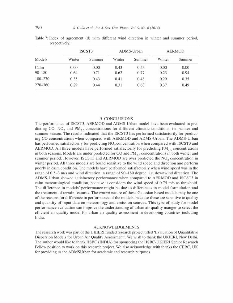
Table 7: Index of agreement (d) with different wind direction in winter and summer period, respectively.
Models
ISCST3 ADMS-Urban AERMOD
Winter Summer Winter Summer Winter Summer
Calm 0.00 0.00 0.43 0.53 0.00 0.0090–180 0.64 0.71 0.62 0.77 0.23 0.94
180–270 0.35 0.43 0.41 0.48 0.29 0.35
270–360 0.29 0.44 0.31 0.63 0.37 0.49
5 CONCLUSIONSThe performance of ISCST3, AERMOD and ADMS-Urban model have been evaluated in pre-dicting CO, NO2 and PM2.5 concentrations for different climatic conditions, i.e. winter and summer season. The results indicated that the ISCST3 has performed satisfactorily for predict-ing CO concentrations when compared with AERMOD and ADMS-Urban. The ADMS-Urban has performed satisfactorily for predicting NO2 concentration when compared with ISCST3 and AERMOD. All three models have performed satisfactorily for predicting PM2.5 concentrations in both seasons. Models are under predicted for CO and PM2.5 concentrations in both winter and summer period. However, ISCST3 and AERMOD are over predicted the NO2 concentration in winter period. All three models are found sensitive to the wind speed and direction and perform poorly in calm condition. The models have performed satisfactorily when wind speed was in the range of 0.5–3 m/s and wind direction in range of 90–180 degree, i.e. downwind direction. The ADMS-Urban showed satisfactory performance when compared to AERMOD and ISCST3 in calm meteorological condition, because it considers the wind speed of 0.75 m/s as threshold. The difference in models’ performance might be due to differences in model formulation and the treatment of terrain features. The causal nature of these Gaussian based models may be one of the reasons for difference in performance of the models, because these are sensitive to quality and quantity of input data on meteorology and emission sources. This type of study for model performance evaluation can improve the understanding of urban air quality manger to select the effi cient air quality model for urban air quality assessment in developing countries including India.
ACKNOWLEDGEMENTSThe research work was part of the UKIERI funded research project titled ‘Evaluation of Quantitative Dispersion Models for Urban Air Quality Assessment’. We wish to thank the UKIERI, New Delhi. The author would like to thank HSBC (INDIA) for sponsoring the HSBC-UKIERI Senior Research Fellow position to work on this research project. We also acknowledge with thanks the CERC, UK for providing us the ADMSUrban for academic and research purposes.
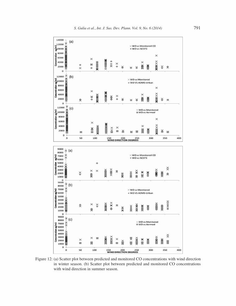
S. Gulia et al., Int. J. Sus. Dev. Plann. Vol. 9, No. 6 (2014) 791
Figure 12: (a) Scatter plot between predicted and monitored CO concentrations with wind direction in winter season. (b) Scatter plot between predicted and monitored CO concentrations with wind direction in summer season.

792 S. Gulia et al., Int. J. Sus. Dev. Plann. Vol. 9, No. 6 (2014)
REFERENCES[1] Gurjar, B.R., Butler, T.M., Lawrence, M.G. & Lelieveld, J., Evaluation of emissions and air
quality in megacities. Atmospheric Environment, 42, pp. 1593–1606, 2008. doi: http://dx.doi.org/10.1016/j.atmosenv.2007.10.048
[2] Baldasano, J.M., Valera, E. & Jimenez, P., Air quality data from large cities. The Science of the Total Environment, 307, pp. 141–165, 2003. doi: http://dx.doi.org/10.1016/s0048-9697(02)00537-5
[3] Mayer, H., Air pollution in cities. Atmospheric Environment, 33, pp. 4029–4037, 1999. doi: http://dx.doi.org/10.1016/s1352-2310(99)00144-2
[4] Nagendra, S., Khare, M., Gulia, S., Vijay, P., Chithra, V.S., Bell, M. & Namdeo, A., Applica-tion of ADMS and AERMOD models to study the dispersion of vehicular pollutants in urban areas of India and the United Kingdom. 20th WIT international conference on Air Pollution at Coruna, Spain, doi:10.2495/AIR120011, 2012. doi: http://dx.doi.org/10.2495/air120011
[5] Sharma, N., Chaudhry, K.K. & Rao, C.V.C., Vehicular pollution modelling in India. Journal of the Institution of Engineers (India), 85, pp. 46–63, 2005.
[6] Badami, M.G., Urban transport policy as if people and the environment mattered: pedestrian accessibility the fi rst step. Economic & Political Weekly, XLIV(33), pp. 43–51, 2009.
[7] CPCB, Status of vehicular pollution control program in India, Program Objective Series/PROBES/136, 2010.
[8] Longhurst, J.W.S., Lindley, S.J., Watson, A.F.R. & Conlan, D.E., The introduction of local air quality management in the United Kingdom: a review and theoretical framework. Atmospheric Environment, 30, pp. 3975–3985, 1996. doi: http://dx.doi.org/10.1016/1352-2310(96)00114-8
[9] Nagendra, S.M.S. & Khare, M., Line source emission modelling- review. Atmospheric Envi-ronment, 36(13), pp. 2083–2098, 2002. doi: http://dx.doi.org/10.1016/s1352-2310(02)00177-2
[10] CAI-Asia Centre, Country synthesis report on urban air quality management for India. Asian Development Bank and the Clean Air Initiative for Asian Cities (CAI-Asia) Center, 2006.
[11] Majumdar, B.K., Dutta, A., Chakrabarty, S. & Ray, S., Correction factors of CALINE 4: a study of automobile pollution in Kolkata. Indian Journal of Air Pollution Control, 8(1), pp. 1–7, 2008.
[12] Bhanarkar, A.D., Goyal, S.K., Sivacoumar, R. & Rao, C.V.C., Assessment of contribution of SO2 and NO2 from different sources in Jamshedpur region, India. Atmospheric Environment, 39, pp. 7745–7760, 2005. doi: http://dx.doi.org/10.1016/j.atmosenv.2005.07.070
[13] U.S. Environment Protection Agency, Federal Register, Part-III, 40 CFR Part 51, Revisions to the guideline on air quality models: Adoption of a Preferred General Purpose (Flat and Com-plex Terrain) Dispersion Model and Other Revisions; Final Rule, 2005.
[14] Carruthers, D.J., Blair, J.W. & Johnson, K.L., Validation and sensitivity study of the ADMS-Urban, TR – 0191, 2003.
[15] Khare, M., Nagendra, S. & Gulia, S., Performance evaluation of air quality dispersion mod-els at urban intersection of an Indian city: a case study of Delhi city. 20th WIT International Conference on Air Pollution at Coruna, Spain, 157, pp. 249–259, 2012. doi: http://dx.doi.org/10.2495/air120221
[16] Kumar, A., Dixit, S., Varadarajan, C., Vijayan, A. & Masuraha, A., Evaluation of the AERMOD dispersion model as a function of atmospheric stability for an urban area. Environmental Prog-ress, 25(2), pp. 141–151, 2006. doi: http://dx.doi.org/10.1002/ep.10129
[17] Long, E.L., Cordova, F.J. & Tanrikulu, S., An analysis of AERMOD sensitivity to input parameters in the San Francisco Bay Area. 13th Conference on the Applications of Air Pollu-

S. Gulia et al., Int. J. Sus. Dev. Plann. Vol. 9, No. 6 (2014) 793
tion Meteorology with the Air and Waste Management Association, American Meteorological Society, Vancouver, BC, August, 23–25, 2004.
[18] Faulkner, W.B., Shaw, B.W. & Grosch, T., Sensitivity of two dispersion models (AERMOD and ISCST3) to input parameters for a rural ground-level area source. Air & Waste Manage. Assoc., 58, pp. 1288–1296, 2008. doi: http://dx.doi.org/10.3155/1047.3289.58.10.1288
[19] Cambridge Environmental Research Consultants, ADMS-Urban model user guide, 2006.[20] Mohan, M., Bhati, S. & Marrapu, P., Performance evaluation of AERMOD and ADMS-Urban
models in a tropical urban environment. Indian Journal of Air pollution Control, 9(1), pp. 47–62, 2009.
[21] Cimorelli, A.J., Perry, S.G., Venkatram, A., Weil, J.C., Paine, R.J., Wilson, R.B., Lee, R.F., Peters, W.D. & Brod, R.W., AERMOD: a dispersion model for industrial source applications. Part I: General model formulation and boundary layer characterization. Journal of Applied Meteorology, 44, pp. 683–693, 2005. doi: http://dx.doi.org/10.1175/jam2227.1
[22] Carruthers, D.J., Blair, J.W. & Johnson, K.L., Validation and sensitivity study of the ADMS-Urban for London. Cambridge Environmental Research Consultants. FM489/R5, 2003.
[23] USEPA, User’s Guide for the Industrial Source Complex (ISC3) Dispersion Model (Revised). Volume II - Description of Model Algorithms. EPA-454/b-95-0036, 1995.
[24] Mohan, M. & Kandya, A., An analysis of annual and seasonal trends of air quality index of Delhi. Environmental Monitoring and Assessment, 131, pp. 267–277, 2007. doi: http://dx.doi.org/10.1007/s10661-006-9474-4
[25] Central Pollution Control Board, National ambient air quality status report, www.cpcb.nic.in, 2007.
[26] Goyal, P., Jaiswal, N., Kumar, A., Dadoo, J.K. & Dwarakanath, M., Air quality impact assess-ment of NOx and PM due to diesel vehicles in Delhi. Transportation Research Part D, 15, pp. 298–303, 2010. doi: http://dx.doi.org/10.1016/j.trd.2010.03.002
[27] CRRI, Multi-Scale Modelling Platform for Environment Forecasting and Management (CMM0020) (Emission Modelling Component), Central Road Research Institute: New Delhi, 2007.
[28] ARAI, Emission Factor Development for Indian Vehicles. Project Report No.AEF/2006-07/IOCL/Emission Factor Project, Automotive Research Association of India: Pune, 2007.
[29] Aneja, V.P., Agrawal, A., Roelle, P.A., Philips, S.B., Tong, Q. & Watkins, N., Measurement and analysis of criteria pollutants in New Delhi, India. Environmental Modelling & Software, 27(1), pp. 35–42, 2001. doi: http://dx.doi.org/10.1016/s0160-4120(01)00051-4