Ordinary Differential Equations

Francisco Esquembre, Universidad de Murcia, SpainWolfgang Christian, Davidson College, NC, USA

July 13, 2007

1 Introduction

Right from the invention of calculus, ordinary differential equations (ODEs)have been used to model continuous systems in all scientific and engineeringdisciplines. The idea is simple in principle and applies to physical situations inwhich information can be obtained about the continuous rate of change of thestate variables of the system. The hope is that we will be able to ascertain theevolution of the system using this information and the knowledge of its initialstate.

We first consider some examples from different disciplines.The simple pendulum. A simple pendulum is a physical abstraction in

which a point mass m oscillates in a vertical plane at the end of a rod of lengthL with negligible mass. The motion of a simple pendulum can be modeled bythe ODE:

mL2θ(t) + bθ(t) + mgL sin θ(t) = τe(t), (1)

where θ(t) is the angular position of the rod of the pendulum with respect tothe vertical, b is the friction coefficient, g is the acceleration due to gravity, andτe(t) is a time-dependent external torque which drives the motion. Typically,the pendulum starts at time t = 0 from a given angle θ0 with zero initial angularvelocity.

Dynamics of chemical reactions. The Brusselator was proposed in 1968by R. Lefever and the Nobel Prize winner I. Prigogine, as a model for an auto-catalytic, oscillating chemical reaction. The mechanism for the reaction is givenby:

Ak1−→ X (2a)

B + Xk2−→ Y + C (2b)

2X + Yk3−→ 3X (2c)

Xk4−→ D . (2d)

We are interested in the evolution of the intermediate products, X and Y . Ifwe assume that the concentration of the reactants A and B is kept constant,

1

a = [A] and b = [B], and denote x = [X] and y = [Y ], the system is describedby the differential equations:

x(t) = k1a− k2bx(t) + k3x2(t)y(t)− k4x(t) (3a)

y(t) = k2bx(t)− k3x2(t)y(t) (3b)

The initial value of x and y is zero. For appropriate values of the parameters,this system can exhibit oscillatory behavior.

Predator-prey population dynamics. ODEs are frequently used in biol-ogy to model population dynamics. The famous Lotka-Volterra model describesthe evolution of two species, one of which preys (feeds) on the other, using theODEs:

x1(t) = ax1(t)− bx1(t)x2(t) (4a)x2(t) = cx1(t)x2(t)− dx2(t) . (4b)

Here, x1 represents the number of prey and x2 is the number of predators (inappropriate units so that they take continuous values in the interval [0, 1]),and a, b, c, and d are parameters. The terms ax1 and −dx2 account for thereproduction rate of each species in the absence of interaction with the otherand the nonlinear terms represent the effects of predation on the reduction ofprey and the reproduction of the predators. This model was used in the mid1920’s to study how the intensity of fishing affected the different fish populationsin the Mediterranean Sea.

Planetary motion. Kepler discovered his three laws of planetary motionafter a titanic analysis of years of astronomical observations by Tycho Brahe.Newton’s inverse-square law of gravitation allows us to reformulate this motionin modern terms using the equations for a massless test particle about a particleof mass M located at the origin:

x(t) = −GMx(t)

(x2(t) + y2(t))3/2(5a)

y(t) = −GMy(t)

(x2(t) + y2(t))3/2(5b)

where M is the combined mass of the Sun and the planet and G is the universalgravitational constant. The xy-coordinates for the massless test particle are therelative position of the planet with respect to the Sun in this two-body approx-imation of the solar system. The initial values for x and y and its derivativesare taken from direct astronomical observation.

The examples presented here are typical. Formulating the problem withthe help of ODEs and stating the existence and uniqueness of a solution un-der reasonable regularity conditions are relatively easy tasks. But finding ananalytic solution is often difficult and might be impossible. Although analyticsolutions, such as in the case of linear ODEs, are very important theoretically,the vast majority of problems cannot be solved in this manner. In these cases,

2

we must use numerical techniques to approximate the evolution of our model.This chapter introduces some of these techniques.

The numerical algorithms we will discuss can be implemented in many dif-ferent ways, using almost any programming language. We have chosen Javato illustrate particular algorithmic implementations. Java is an object-orientedprogramming language that is designed to run on a virtual computer that canbe implemented for any modern operating system. This promise of platformindependence has become a reality, and we now can write programs that haveattractive graphical user interfaces and support common tasks such as printing,disk access, and copy-paste data exchange with other applications.

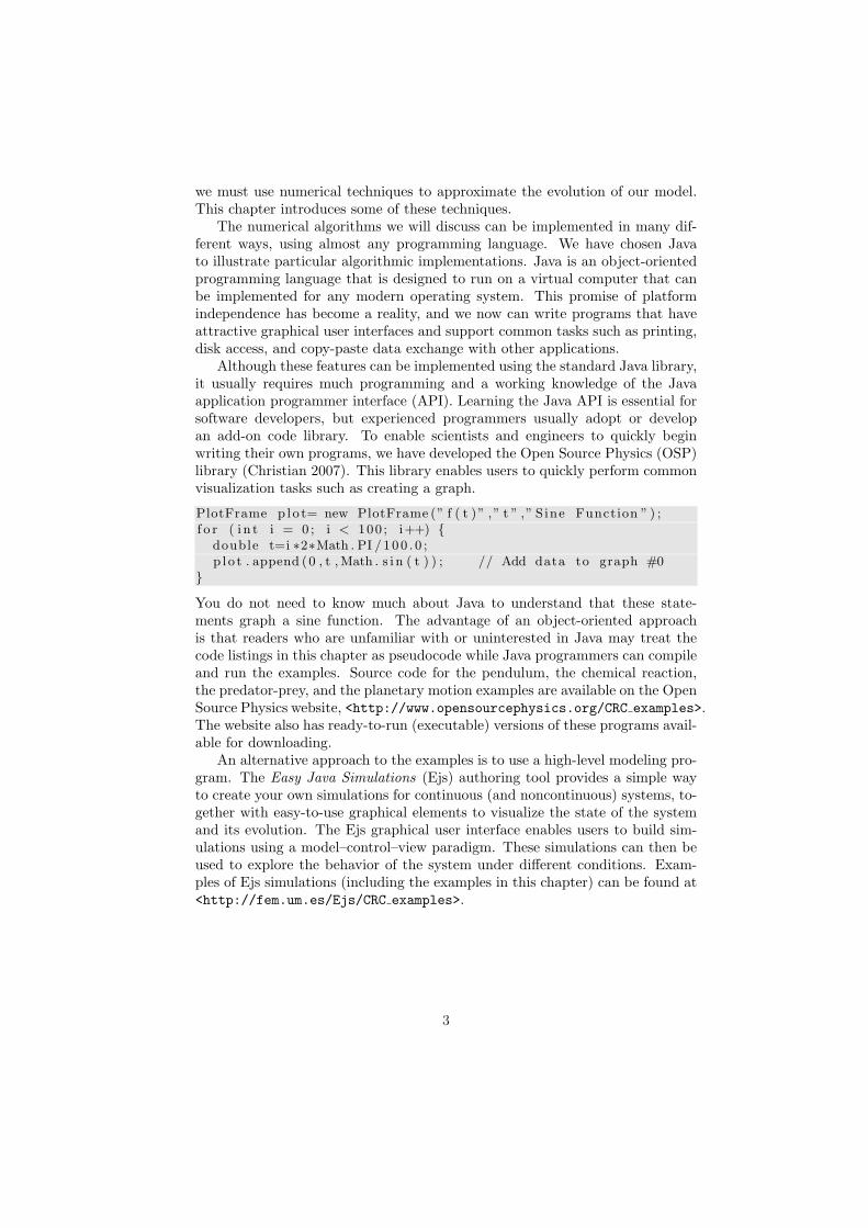
Although these features can be implemented using the standard Java library,it usually requires much programming and a working knowledge of the Javaapplication programmer interface (API). Learning the Java API is essential forsoftware developers, but experienced programmers usually adopt or developan add-on code library. To enable scientists and engineers to quickly beginwriting their own programs, we have developed the Open Source Physics (OSP)library (Christian 2007). This library enables users to quickly perform commonvisualization tasks such as creating a graph.

PlotFrame p lo t= new PlotFrame (” f ( t )” ,” t ” ,” Sine Function ” ) ;f o r ( i n t i = 0 ; i < 100 ; i++) {

double t=i ∗2∗Math . PI /100 . 0 ;p l o t . append (0 , t , Math . s i n ( t ) ) ; // Add data to graph #0

}You do not need to know much about Java to understand that these state-ments graph a sine function. The advantage of an object-oriented approachis that readers who are unfamiliar with or uninterested in Java may treat thecode listings in this chapter as pseudocode while Java programmers can compileand run the examples. Source code for the pendulum, the chemical reaction,the predator-prey, and the planetary motion examples are available on the OpenSource Physics website, <http://www.opensourcephysics.org/CRC examples>.The website also has ready-to-run (executable) versions of these programs avail-able for downloading.

An alternative approach to the examples is to use a high-level modeling pro-gram. The Easy Java Simulations (Ejs) authoring tool provides a simple wayto create your own simulations for continuous (and noncontinuous) systems, to-gether with easy-to-use graphical elements to visualize the state of the systemand its evolution. The Ejs graphical user interface enables users to build sim-ulations using a model–control–view paradigm. These simulations can then beused to explore the behavior of the system under different conditions. Exam-ples of Ejs simulations (including the examples in this chapter) can be found at<http://fem.um.es/Ejs/CRC examples>.

3

2 Numerical Solution

The mathematical formulation most frequently used in modeling continuoussystems is that of an initial-value problem for a first-order ordinary differentialequation. 1 An initial-value problem is an expression of the form:

x(t) = f(x(t), t), x(a) = x0 . (6)

In this expression, t (which often represents the time) is called the independentvariable and can take values in a given interval [a, b] of the real line, x(t) rep-resents a k-dimensional vector of real numbers that describes the state of thesystem at a given instant, and the vector function f conveys all the informationthat relates the rate of change of the state vector with the value of the inde-pendent variable and the state itself. The information provided at the initialinstant of time, x(a) = x0, is called the initial condition, and is necessary tocompletely determine a solution out of the many possible solutions.

ODEs in which the right-hand side has no explicit dependence on time,x(t) = f(x(t)), are called autonomous and are of interest because they describedynamical systems, systems whose dynamics depend only on their internal state,independently on the instant of time at which it is measured. Nonautonomousequations contain an explicit time dependence, x(t) = f(x(t), t). The simplependulum in Section 1 is an example of a nonautonomous equation, while allothers describe dynamical systems.

Every nonautonomous ODE can be reformulated as a dynamical system byadding the time to the system of differential equations. That is, we add theindependent variable t to the state vector x = (x(t), t) and we add rate dt/dt =1 to the rate f = (f(x, t), 1). Although adding another variable makes thegeometrical interpretation more difficult, it is inconsequential (and sometimesmore convenient) from a computational point of view. We will use this approachin our implementation code.

We have chosen to represent the dynamical system state (x1, x2, x3, . . . , xk, t)as a vector because most interesting phenomena involve multiple state variables.Even in cases where the state can be described by a single number, derivativesof order higher than one usually appear. For instance, a typical physics model,such as the pendulum, obeys Newton’s second law F = ma, which is a second-order differential equation. These cases are contained in our definition above,because any higher order differential equation can be rewritten as a new first-order ODE. As an example, we can construct a system of first-order differentialequations from Equation (1) by introducing a velocity ω for the angle θ. Thedriven pendulum can then be written as the following coupled nonautonomous

1ODEs can also appear in the form of boundary value problems, where the informationabout the state of the system is provided partly in one initial instant of time, and partly inone final instant of time (Press, Teukolsky, Vetterling, and Flannery 1992; Keller 1992).

4

system of first-order differential equations for the variables (θ, ω, t):

θ = ω (7a)

ω = − g

Lsin(θ)− b

mL2ω +

1mL2

τe(t) (7b)

t = 1. (7c)

The numerical solution of ordinary differential equations is a well-studiedproblem in numerical analysis. Practically all numerical techniques are basedon difference methods. In these methods, we attempt to obtain approximatevalues of the solution at a sequence of mesh points a = t0 < t1 < . . . < tN = b.Although obtaining a solution at a finite number of mesh points appears restric-tive, the idea is actually very useful. In many cases, scientists and engineers usemodels to study how systems evolve in time by simulating them with differentparameters and initial conditions, plotting or displaying the state of the systemat regular time steps. This is precisely what difference methods do.

Solving differential equations numerically is both a science and an art. Thereexist many authoritative books on the subject, both because the discipline isvery mathematically advanced, and because not all problems behave the same.A universal solving method for ordinary differential equations does not existand practitioners should select a method based on requirements such as speed,accuracy, and the conservation of important physical properties such as energy.

The numerical methods most frequently used fall into the following cate-gories: Taylor methods, Runge–Kutta methods, multistep methods, and ex-trapolation methods. We concentrate on Taylor and Runge–Kutta methodsfirst because they work well in many situations and are easy to implement (par-ticularly Runge–Kutta methods), and because they will help us illustrate themain concepts and details for the computer implementation of difference meth-ods. We will discuss other methods in Section 8.

Implementation techniques. The numerical solution of differential equa-tions can be made simpler using object-oriented programming techniques thatseparate the differential equations from the numerical algorithm. The ODE andODESolver interfaces shown in Figure 1 are code files that will be described inSection 5.

Physical Law Differential Equations SolutionODE- ODESolver-

Figure 1: Differential equations can be solved using the ODE interface to definethe equations and the ODESolver interface to define the numerical algorithm.

A Java interface is a list of methods that an object can perform. Note thatJava allows us to define variables using an interface as a variable type. The ODE

5

interface defined in the Open Source Physics library defines methods (similar tosubroutines or functions) that enable us to encapsulate an initial value problemsuch as (6) in a Java class. The ODESolver interface defines methods thatimplement numerical algorithms for solving differential equations. The mostimportant method in ODESolver is the step method which advances the stateof the differential equation. This allows us to write code such as:

ODE ode = new Pendulum ( ) ; // c r e a t e s ODEODESolver s o l v e r = new RK4( ode ) ; / / c r e a t e s numerica l methods o l v e r . i n i t i a l i z e ( 0 . 0 1 ) ; // each step advances by 0 .01f o r ( i n t i =0; i <100; i++) { // advances by 100 s t ep s

s o l v e r . s tep ( ) ;}

In the spirit of object-oriented programming, the details of how the differen-tial equations are defined and solved are hidden in the Pendulum and RK4 objects.This hiding is known as encapsulation and is a hallmark of good object-orienteddesign. A user can solve the pendulum problem using a different numericalalgorithm by creating (instantiating) a different ODESolver. The OSP librarycontains many differential equation algorithms. The user assumes that thesealgorithms have been properly programmed and the library assumes that theuser has obeyed the OSP API.

3 Taylor methods

The first difference method we will study is based on the Taylor series expansionof the solution x(t). Namely,

x(t + h) = x(t) + hx(t) +h2

2!x(t) +

h3

3!x(3)(t) + · · · . (8)

If we know the value of x(t), we can compute x(t) from the differential equation.The second and subsequent derivatives of x at t can be obtained by repeatedlydifferentiating (6). Thus,

x(t) = ft(x(t), t) + fx(x(t), t) f(x(t), t) (9)

and similarly for higher-order derivatives. Notice however, that the expressionbecomes more complicated as we compute higher order derivatives.

Because we actually know from (6) the value of x at t0, we can take h0 =t1 − t0, and use a Taylor expansion to obtain u1, an approximation to x(t1).We can now use u1 to repeat the process with h1 = t2 − t1 and obtain anapproximation of x(t2), u2, and so on until we reach tN .

Consider again the example of the simple pendulum (with no external torque,for simplicity). By repeatedly differentiating (7) and applying the described

6

numerical scheme, we obtain the coupled recurrent sequences:

θn+1 = θn + hnωn +h2

n

2!

[− g

Lsin(θn)− b

mL2ωn

]+ . . . (10a)

ωn+1 = ωn + hn

[− g

Lsin(θn)− b

mL2ωn

]

+h2

n

2!

[− g

Lcos(θn)ωn +

b

mL2

g

Lsin(θn) +

(b

mL2

)2

ωn

]+ · · · (10b)

tn+1 = tn + hn (10c)

for n = 0, 1, . . . , N − 1, where t0 = 0, θ0 = θ(0), and ω0 = 0.Implementing such an iterative procedure on a computer is straightforward.

We only need to choose the number of terms in the Taylor expansion that wewill use, and the appropriate values for the mesh points tn. The typical choiceis to choose first N (the number of steps), and then take all tn equally spacedin the interval [a, b]. This choice leads to hn = h = (b− a)/N , for all n.

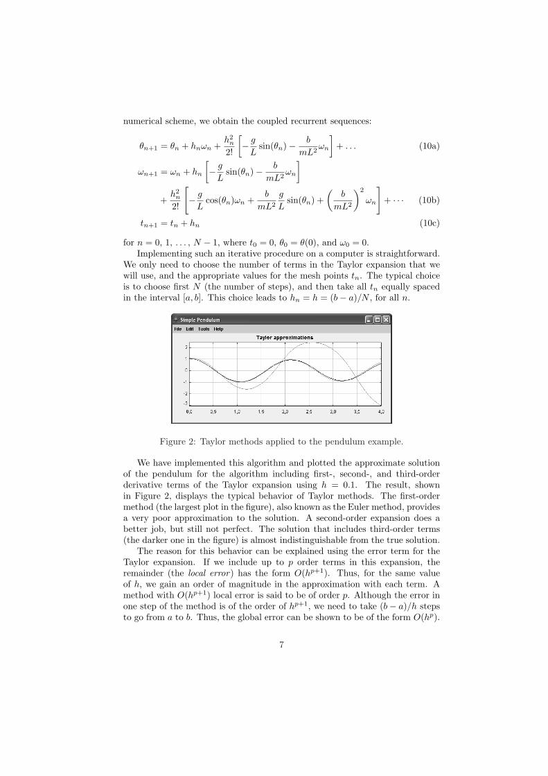
Figure 2: Taylor methods applied to the pendulum example.

We have implemented this algorithm and plotted the approximate solutionof the pendulum for the algorithm including first-, second-, and third-orderderivative terms of the Taylor expansion using h = 0.1. The result, shownin Figure 2, displays the typical behavior of Taylor methods. The first-ordermethod (the largest plot in the figure), also known as the Euler method, providesa very poor approximation to the solution. A second-order expansion does abetter job, but still not perfect. The solution that includes third-order terms(the darker one in the figure) is almost indistinguishable from the true solution.

The reason for this behavior can be explained using the error term for theTaylor expansion. If we include up to p order terms in this expansion, theremainder (the local error) has the form O(hp+1). Thus, for the same valueof h, we gain an order of magnitude in the approximation with each term. Amethod with O(hp+1) local error is said to be of order p. Although the error inone step of the method is of the order of hp+1, we need to take (b− a)/h stepsto go from a to b. Thus, the global error can be shown to be of the form O(hp).

7

The approximation described above can also be improved for any order byreducing the value of h. However, reducing h increases both the computationaleffort and the round-off error. Thus, we will need to balance the order of themethod with the right value of h for our problem.

4 Runge–Kutta methods

Although methods based on a Taylor series expansion can be made very ac-curate by taking sufficiently many terms, computing higher-order derivativesbecomes increasingly complicated and the resulting code cannot be reused for adifferent problem. For this reason, numerical analysts have developed methodswith similar accuracy that are easier to implement and reuse. In particular,these methods only require evaluations of the function f which defines the dif-ferential equation. The Runge–Kutta methods described here are among themost popular.

Whereas Taylor methods advance the solution by evaluating f and its deriva-tives at a single point, Runge–Kutta methods advance the solution un by eval-uating f at several intermediate points in the interval [tn, tn+1]. These interme-diate results are combined in such a way as to match the Taylor expansion ofthe solution up to a given order. The precise formulation of a s-stage explicitRunge–Kutta method is the following:

k1 = f(un, tn)k2 = f(un + hna21k1, tn + c2hn)· · ·

ks = f(un + hn(as1k1 + · · ·+ as,s−1ks−1), tn + cshn)un+1 = un + hn(b1k1 + b2k2 + · · ·+ bsks).

(11)

Note that the method describes a simple recurrent algorithm, which is easy toimplement on a computer and requires only the evaluation of the function f .The method is determined by the parameters, which are listed traditionally inform of a table (Table 1). Usually, the ci satisfy the condition: ci =

∑i−1j=1 aij .

0c2 a21

c3 a31 a32

......

.... . .

cs as1 as2 · · · as,s−1

b1 b2 · · · bs−1 bs

Table 1: Generic Runge–Kutta table of coefficients.

For a given s, the algorithm consists of choosing appropriate values of thea, b, and c parameters which provide a good approximation of the solution.

8

The case s = 2 illustrates the procedure. Consider the second-order Taylorapproximation of the solution at tn given by:

x(tn + hn) = x(tn) + hnf +h2

n

2!(ft + fx f) + O(h3

n), (12)

where f and its derivatives are evaluated at (x(tn), tn). If we expand the valueof the approximation produced by the method (11) for s = 2 and use the Taylorexpansion of the function f , we find that:

un+1 = un + hn[b1f(un, tn) + b2f(un + hna21f(un, tn), tn + c2hn)]

= un + hnb1f + hnb2 (f + hnc2ft + hna21fx f) + O(h3n)

= un + hn(b1 + b2)f + h2n (b2c2ft + b2a21fx f) + O(h3

n).

(13)

Except where explicitly indicated, f and its derivatives are evaluated at (un, tn).Hence, if un is a good approximation of x(tn), the method will approximate thesolution at tn + hn with a third-order local error (which leads to a second-order method) if b1 + b2 = 1, b2c2 = 1/2, and b2a21 = 1/2. Because we havefour unknowns and only three equations, this expression gives a one-parameterfamily of methods for Runge–Kutta algorithms of order two. The most popularare the following:

(Heun’s method)

un+1 = un +hn

2[f(un, tn) + f(un + hnf(un, tn), tn + hn)] , (14)

(Midpoint method)

un+1 = un + hnf(un +hn

2f(un, tn), tn +

hn

2), (15)

(Ralston’s method)

un+1 = un +hn

3

[f(un, tn) + 2f(un +

34hnf(un, tn), tn +

34hn)

], (16)

which correspond to b1 = 1/2, b1 = 0, and b1 = 1/3, respectively.The same approach can be used to obtain families of higher order Runge–

Kutta methods, although the algebra becomes much more complicated andmore sophisticated techniques must be used (Hairer, Nørsett, and Wanner 2000;Butcher 1987).

The best-seller of all Runge–Kutta methods is the fourth-order classicalmethod given by Table 2, which requires four rate evaluations per step. But thismethod is certainly not the end of the story, and we will give higher-order meth-ods in Section 6. However, for orders five and above, all Runge–Kutta methodsrequire a number of stages strictly greater than the order. This limitation isone of the Butcher’s barriers.

9

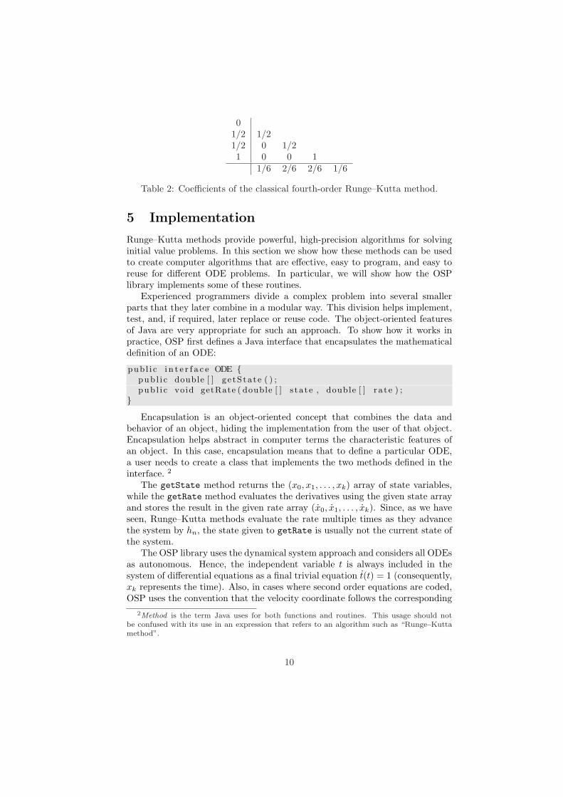
01/2 1/21/2 0 1/21 0 0 1

1/6 2/6 2/6 1/6

Table 2: Coefficients of the classical fourth-order Runge–Kutta method.

5 Implementation

Runge–Kutta methods provide powerful, high-precision algorithms for solvinginitial value problems. In this section we show how these methods can be usedto create computer algorithms that are effective, easy to program, and easy toreuse for different ODE problems. In particular, we will show how the OSPlibrary implements some of these routines.

Experienced programmers divide a complex problem into several smallerparts that they later combine in a modular way. This division helps implement,test, and, if required, later replace or reuse code. The object-oriented featuresof Java are very appropriate for such an approach. To show how it works inpractice, OSP first defines a Java interface that encapsulates the mathematicaldefinition of an ODE:

pub l i c i n t e r f a c e ODE {pub l i c double [ ] g e tS ta t e ( ) ;pub l i c void getRate ( double [ ] s ta te , double [ ] r a t e ) ;

}Encapsulation is an object-oriented concept that combines the data and

behavior of an object, hiding the implementation from the user of that object.Encapsulation helps abstract in computer terms the characteristic features ofan object. In this case, encapsulation means that to define a particular ODE,a user needs to create a class that implements the two methods defined in theinterface. 2

The getState method returns the (x0, x1, . . . , xk) array of state variables,while the getRate method evaluates the derivatives using the given state arrayand stores the result in the given rate array (x0, x1, . . . , xk). Since, as we haveseen, Runge–Kutta methods evaluate the rate multiple times as they advancethe system by hn, the state given to getRate is usually not the current state ofthe system.

The OSP library uses the dynamical system approach and considers all ODEsas autonomous. Hence, the independent variable t is always included in thesystem of differential equations as a final trivial equation t(t) = 1 (consequently,xk represents the time). Also, in cases where second order equations are coded,OSP uses the convention that the velocity coordinate follows the corresponding

2Method is the term Java uses for both functions and routines. This usage should notbe confused with its use in an expression that refers to an algorithm such as “Runge–Kuttamethod”.

10

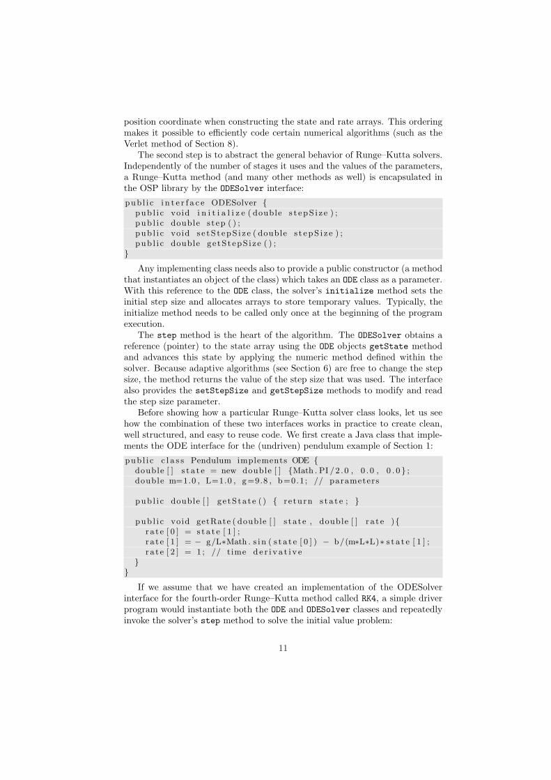
position coordinate when constructing the state and rate arrays. This orderingmakes it possible to efficiently code certain numerical algorithms (such as theVerlet method of Section 8).

The second step is to abstract the general behavior of Runge–Kutta solvers.Independently of the number of stages it uses and the values of the parameters,a Runge–Kutta method (and many other methods as well) is encapsulated inthe OSP library by the ODESolver interface:

pub l i c i n t e r f a c e ODESolver {pub l i c void i n i t i a l i z e ( double s t epS i z e ) ;pub l i c double s tep ( ) ;pub l i c void s e tS t epS i z e ( double s t epS i z e ) ;pub l i c double ge tS t epS i z e ( ) ;

}Any implementing class needs also to provide a public constructor (a method

that instantiates an object of the class) which takes an ODE class as a parameter.With this reference to the ODE class, the solver’s initialize method sets theinitial step size and allocates arrays to store temporary values. Typically, theinitialize method needs to be called only once at the beginning of the programexecution.

The step method is the heart of the algorithm. The ODESolver obtains areference (pointer) to the state array using the ODE objects getState methodand advances this state by applying the numeric method defined within thesolver. Because adaptive algorithms (see Section 6) are free to change the stepsize, the method returns the value of the step size that was used. The interfacealso provides the setStepSize and getStepSize methods to modify and readthe step size parameter.

Before showing how a particular Runge–Kutta solver class looks, let us seehow the combination of these two interfaces works in practice to create clean,well structured, and easy to reuse code. We first create a Java class that imple-ments the ODE interface for the (undriven) pendulum example of Section 1:

pub l i c c l a s s Pendulum implements ODE {double [ ] s t a t e = new double [ ] {Math . PI /2 . 0 , 0 . 0 , 0 . 0 } ;double m=1.0 , L=1.0 , g=9.8 , b=0.1 ; // parameters

pub l i c double [ ] g e tS ta t e ( ) { re turn s t a t e ; }

pub l i c void getRate ( double [ ] s ta te , double [ ] r a t e ){r a t e [ 0 ] = s t a t e [ 1 ] ;r a t e [ 1 ] = − g/L∗Math . s i n ( s t a t e [ 0 ] ) − b/(m∗L∗L)∗ s t a t e [ 1 ] ;r a t e [ 2 ] = 1 ; // time d e r i v a t i v e

}}

If we assume that we have created an implementation of the ODESolverinterface for the fourth-order Runge–Kutta method called RK4, a simple driverprogram would instantiate both the ODE and ODESolver classes and repeatedlyinvoke the solver’s step method to solve the initial value problem:

11

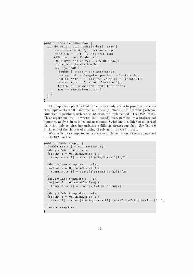
pub l i c c l a s s PendulumMain {pub l i c s t a t i c void main ( St r ing [ ] a rgs ){

double max = 4 ; // s o l u t i o n rangedouble h = 0 . 1 ; // ode step s i z eODE ode = new Pendulum ( ) ;ODESolver od e s o l v e r = new RK4( ode ) ;od e s o l v e r . i n i t i a l i z e (h ) ;whi l e (max>0) {

double [ ] s t a t e = ode . ge tS ta t e ( ) ;S t r ing xStr = ” angular p o s i t i o n = ”+s t a t e [ 0 ] ;S t r ing vStr = ” , angular v e l o c i t y = ”+s t a t e [ 1 ] ;S t r ing tS t r = ” , time = ”+s t a t e [ 2 ] ;System . out . p r i n t ( xStr+vStr+tSt r+”\n ” ) ;max −= ode s o l v e r . s tep ( ) ;

}}

}The important point is that the end-user only needs to program the class

that implements the ODE interface and thereby defines the initial value problem.Numerical algorithms, such as the RK4 class, are implemented in the OSP library.These algorithms can be written (and tested) once, perhaps by a professionalnumerical analyst, in an independent manner. Switching to a different numericalalgorithm only requires instantiating a different ODESolver class. See Table 6at the end of the chapter of a listing of solvers in the OSP library.

We now list, for completeness, a possible implementation of the step methodfor the RK4 method:

pub l i c double s tep ( ) {double s t a t e [ ] = ode . ge tS ta t e ( ) ;ode . getRate ( s ta te , k1 ) ;f o r ( i n t i = 0 ; i<numEqn ; i++) {

temp state [ i ] = s t a t e [ i ]+ s t epS i z e ∗k1 [ i ] / 2 ;}ode . getRate ( temp state , k2 ) ;f o r ( i n t i = 0 ; i<numEqn ; i++) {

temp state [ i ] = s t a t e [ i ]+ s t epS i z e ∗k2 [ i ] / 2 ;}ode . getRate ( temp state , k3 ) ;f o r ( i n t i = 0 ; i<numEqn ; i++) {

temp state [ i ] = s t a t e [ i ]+ s t epS i z e ∗k3 [ i ] ;}ode . getRate ( temp state , k4 ) ;f o r ( i n t i = 0 ; i<numEqn ; i++) {

s t a t e [ i ] = s t a t e [ i ]+ s t epS i z e ∗( k1 [ i ]+2∗k2 [ i ]+2∗k3 [ i ]+k4 [ i ] ) / 6 . 0 ;}re turn s t epS i z e ;

}

12

6 Adaptive step

An important aspect of solving ODEs numerically is that of choosing the bestpossible set of mesh points t0 < . . . < tN mentioned in Section 2. The fixedstep size approach that we have used so far, that is, hn = h = (b − a)/N , isnot always appropriate. The solution of the ODE may vary rapidly in someparts of the [a, b] interval (which requires a small step size), while it may bevery smooth in other parts of it (which allows a larger step size). Taking thesame step size for the entire interval might result in either loss of precision orin an unnecessary waste of computer resources, or both.

Making an appropriate choice of mesh points in advance can be difficult.A detailed analytical study of the local error at different points within theinterval is required. Alternatively, there exist numerical techniques that allowthe computer to estimate this error and automatically compute an appropriatevalue of hn for each integration step. These techniques are, for Runge–Kuttamethods, based on two approaches: interval-halving and embedded formulas.

Interval halving. The first approach consists in using, from each point (un, tn),the same Runge-Kutta method in two parallel computations. The first one ap-plies the method once with a given step size h, while the second uses the methodtwice, each with half this step size, i.e. h/2. We thus obtain two different ap-proximations of the solution at tn + h. Both values are then compared toestimate the error obtained with this step size, to accept or not the solution,and to compute a more appropriated step size (Schilling and Harris 2000).

Although this extrapolation process can be easily programmed, the resultingcode is inefficient. For the case of the fourth-order Runge–Kutta method, wewould need 11 different evaluations of the rate function for each individual stepand would achieve only a fifth-order approximation.

Embedded Runge-Kutta formulas. A more efficient scheme was first dis-covered by Fehlberg, who found a pair of Runge–Kutta formulas which used thesame set of coefficients to provide two approximations of different orders. Thedifference between both approximations can then be used to estimate the errorof the lower order formula, while taking the higher order approximation as thefinal output of the method (this is called local extrapolation).

Since the original Fehlberg scheme, many other embedded formulas havebeen found. The most used ones are the 6-stage formulas of Cash and Karp(Table 3), and the 7-stage formulas of Dormand and Prince (table not provided),which attempt to minimize the error of the local extrapolation approximation.Both methods describe a pair of Runge–Kutta–Fehlberg formulas of order 5and 4. The first row of b coefficients in Table 3 corresponds to the higher orderapproximation, while the second row gives the lower order one. Both Cash–Karpand Dormand–Prince schemes are implemented in the OSP library.

13

01/5 1/53/10 3/40 9/403/5 3/10 −9/10 6/51 −11/54 5/2 −70/27 35/27

7/8 1631/55296 175/512 575/13824 44275/110592 253/409637/378 0 250/621 125/594 0 512/1771

2825/27648 0 18575/48384 13525/55296 277/14336 1/4

Table 3: Coefficients for the embedded Runge–Kutta formulas computed byCash and Karp.

Adapting the step. Once the estimated error is found, the technique con-sists in adapting the step size so that this error keeps within reasonable limits,decreasing the step size if the error is too large, and increasing it if the erroris too small. A popular procedure to compute the new step size h consists inusing the following formula (Press, Teukolsky, Vetterling, and Flannery 1992):

h = Sh

∣∣∣∣∆0

∆1

∣∣∣∣α

(17)

where S is a safety constant (such as 0.9), h is the current step size, ∆0 denotesthe desired accuracy, and ∆1 measures the current accuracy. Finally, α denotesa constant that (for a p-order method) is 1/(p+1) when the step size is increased,and 1/p otherwise.

There are different ways to interpret ∆0 and ∆1 in (17). Usually, ∆1 is takenas the maximum of the absolute values of the components of the estimated error(for embedded formulas, of the difference of both approximations). For ∆0, thesimplest option is to let the user specify a suitable small tolerance, ε. For otherpossibilities, such as including a scaling vector, see (Press, Teukolsky, Vetterling,and Flannery 1992; Hairer, Nørsett, and Wanner 2000; Enright, Higham, Owren,and Sharp 1995).

7 Implementation of adaptive step

Implementing an adaptive algorithm based on a pair of Runge–Kutta embeddedformulas is straightforward. The following code shows how the step methodcan be implemented for the Cash–Karp formulas. Notice that the code includesadditional checks to avoid abrupt changes to the step size. In addition, thealgorithm will return if the required precision cannot be attained.

pub l i c double s tep ( ) {i n t i t e r a t i o n s = 10 ;double currentStep = stepS i ze , e r r o r =0;double s t a t e [ ] = ode . ge tS ta t e ( ) ;ode . getRate ( s ta te , k [ 0 ] ) ; // ge t s the i n i t i a l r a t e

14

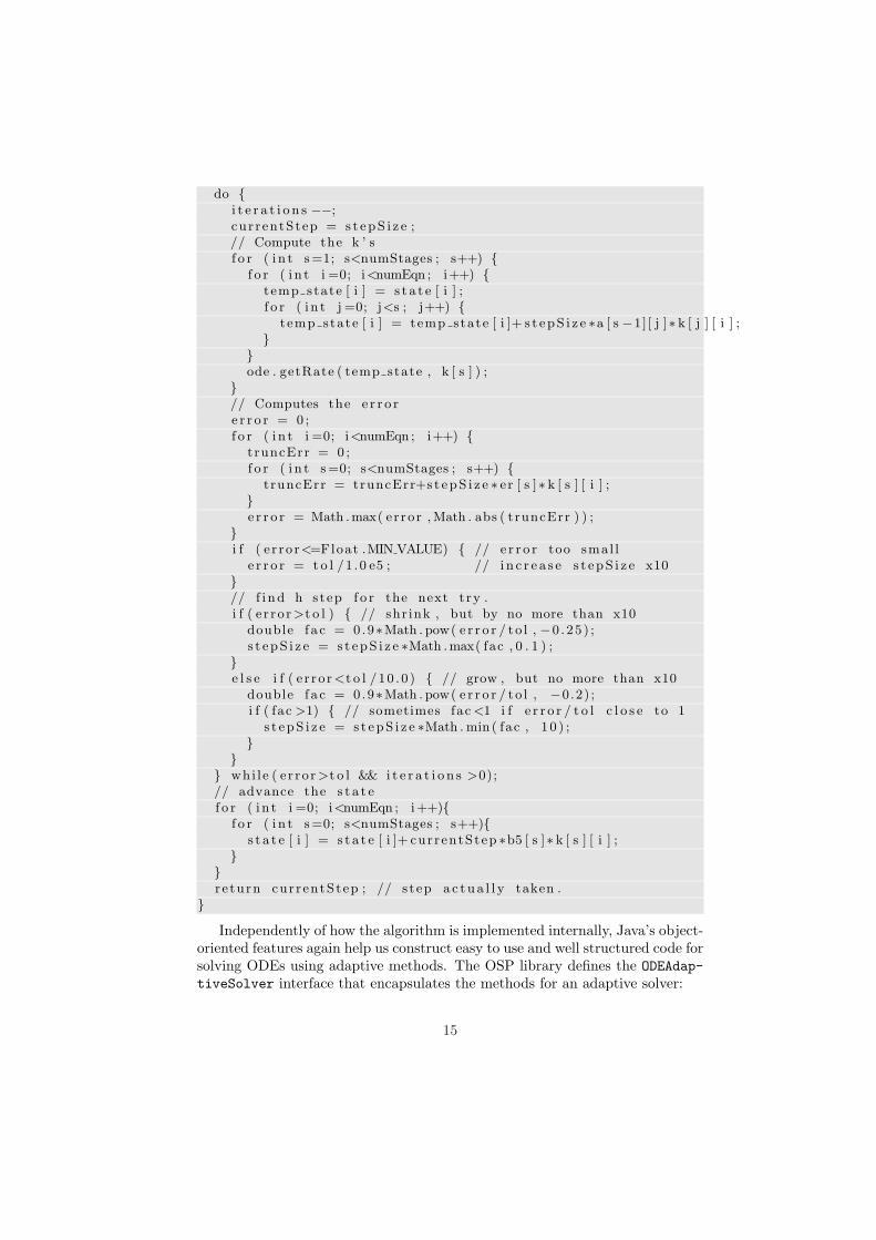
do {i t e r a t i o n s −−;cur rentStep = s t epS i z e ;// Compute the k ’ sf o r ( i n t s=1; s<numStages ; s++) {

f o r ( i n t i =0; i<numEqn ; i++) {temp state [ i ] = s t a t e [ i ] ;f o r ( i n t j =0; j<s ; j++) {

temp state [ i ] = temp state [ i ]+ s t epS i z e ∗a [ s −1] [ j ]∗ k [ j ] [ i ] ;}

}ode . getRate ( temp state , k [ s ] ) ;

}// Computes the e r r o re r r o r = 0 ;f o r ( i n t i =0; i<numEqn ; i++) {

truncErr = 0 ;f o r ( i n t s=0; s<numStages ; s++) {

truncErr = truncErr+s t epS i z e ∗ er [ s ]∗ k [ s ] [ i ] ;}e r r o r = Math .max( er ror , Math . abs ( truncErr ) ) ;

}i f ( e r ro r<=Float .MIN VALUE) { // e r r o r too smal l

e r r o r = t o l /1 .0 e5 ; // i n c r e a s e s t epS i z e x10}// f i nd h step f o r the next t ry .i f ( e r ro r >t o l ) { // shr ink , but by no more than x10

double f a c = 0.9∗Math . pow( e r r o r / to l , −0 .25 ) ;s t epS i z e = s t epS i z e ∗Math .max( fac , 0 . 1 ) ;

}e l s e i f ( e r ror <t o l /10 . 0 ) { // grow , but no more than x10

double f a c = 0.9∗Math . pow( e r r o r / to l , −0.2) ;i f ( fac >1) { // sometimes fac <1 i f e r r o r / t o l c l o s e to 1

s t epS i z e = s t epS i z e ∗Math . min ( fac , 1 0 ) ;}

}} whi le ( e r ror >t o l && i t e r a t i o n s >0);// advance the s t a t ef o r ( i n t i =0; i<numEqn ; i++){

f o r ( i n t s=0; s<numStages ; s++){s t a t e [ i ] = s t a t e [ i ]+ currentStep ∗b5 [ s ]∗ k [ s ] [ i ] ;

}}re turn currentStep ; // s tep a c tua l l y taken .

}Independently of how the algorithm is implemented internally, Java’s object-

oriented features again help us construct easy to use and well structured code forsolving ODEs using adaptive methods. The OSP library defines the ODEAdap-tiveSolver interface that encapsulates the methods for an adaptive solver:

15

pub l i c i n t e r f a c e ODEAdaptiveSolver extends ODESolver {pub l i c void se tTo l e rance ( double t o l ) ;pub l i c double getTolerance ( ) ;

}Because the interface extends the previously defined ODESolver interface, itinherits all the methods defined in this interface. The only new methods arethose that allow the user to specify the desired tolerance (the ε mentionedabove). This interface allows the user to create code such as the following:

ODEAdaptiveSolver od e s o l v e r = new CashKarp45 ( ode ) ;od e s o l v e r . i n i t i a l i z e (h ) ;od e s o l v e r . s e tTo l e rance ( 1 . 0 e−3);

Notice that the only difference with the previous code is in the instantiationof the ODEAdaptiveSolver object, and the addition of a line that sets the desiredtolerance. All other parts of the driver program and the definition of the ODEremain unchanged.

Using an adaptive algorithm can dramatically increase the performance ofour programs in situations where the solution has regions of different behavior.A typical example is that of the computation of the Arenstorf orbits, closedtrajectories of the restricted three-body problem (two bodies of masses µ and1− µ moving in a circular orbit, and a third body of negligible mass moving inthe same plane), such as a satellite-earth-moon system. The equations for themotion of the third body are given by (Hairer, Nørsett, and Wanner 2000):

x1(t) = x1(t) + 2x2(t)− (1− µ)x1(t) + µ

D1− µ

x1(t)− (1− µ)D2

(18a)

x2(t) = x2(t)− 2x1(t)− (1− µ)x2(t)D1

− µx2(t)D2

(18b)

where D1 = ((x1(t) + µ)2 + x22(t))

3/2 and D2 = ((x1(t)− (1− µ))2 + x22(t))

3/2.The Arenstorf orbit for the initial values x1(0) = 0.994, x1(0) = 0, x2(0) = 0,

x2(0) = −2.00158510637908252240537862224, and µ = 0.012277471 is displayedin Figure 3. The grey trajectory has been computed using 3000 fixed-step it-erations of the fourth order Runge–Kutta algorithm (the trajectory is not evenclosed), while the black, closed trajectory has been computed by the adaptiveCash–Karp algorithm with a tolerance of 10−5 in 123 steps with 98 steps ac-cepted and 25 steps rejected. The fact that the second algorithm is of order 5is secondary. Comparing the total number of rate evaluations (12000 vs. 713)shows that the adaptive method is far superior.

Multistepping. Given the relatively small additional effort required to com-pute two Runge–Kutta solutions and thereby to control the error, is there anyreason to use a non-adaptive algorithm? Sometimes. Adaptive algorithms donot work if the rate contains discontinuous functions. A fixed step size is alsoconvenient if the output is to have evenly spaced values.

16

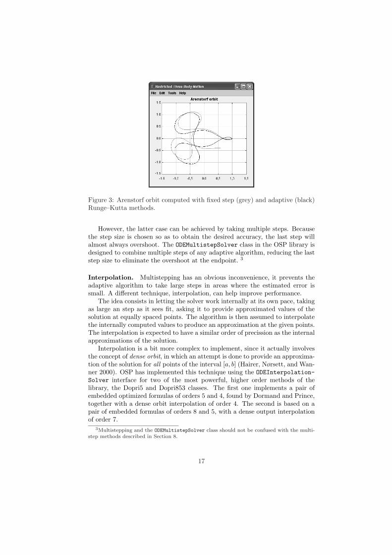
Figure 3: Arenstorf orbit computed with fixed step (grey) and adaptive (black)Runge–Kutta methods.

However, the latter case can be achieved by taking multiple steps. Becausethe step size is chosen so as to obtain the desired accuracy, the last step willalmost always overshoot. The ODEMultistepSolver class in the OSP library isdesigned to combine multiple steps of any adaptive algorithm, reducing the laststep size to eliminate the overshoot at the endpoint. 3

Interpolation. Multistepping has an obvious inconvenience, it prevents theadaptive algorithm to take large steps in areas where the estimated error issmall. A different technique, interpolation, can help improve performance.

The idea consists in letting the solver work internally at its own pace, takingas large an step as it sees fit, asking it to provide approximated values of thesolution at equally spaced points. The algorithm is then assumed to interpolatethe internally computed values to produce an approximation at the given points.The interpolation is expected to have a similar order of precission as the internalapproximations of the solution.

Interpolation is a bit more complex to implement, since it actually involvesthe concept of dense orbit, in which an attempt is done to provide an approxima-tion of the solution for all points of the interval [a, b] (Hairer, Nørsett, and Wan-ner 2000). OSP has implemented this technique using the ODEInterpolation-Solver interface for two of the most powerful, higher order methods of thelibrary, the Dopri5 and Dopri853 classes. The first one implements a pair ofembedded optimized formulas of orders 5 and 4, found by Dormand and Prince,together with a dense orbit interpolation of order 4. The second is based on apair of embedded formulas of orders 8 and 5, with a dense output interpolationof order 7.

3Multistepping and the ODEMultistepSolver class should not be confused with the multi-step methods described in Section 8.

17

These two ODE solvers are available in the Open Source Physics library andcan be created using factory methods as the code below shows.

ODEAdaptiveSolver dopr i5=ODEInterpolat ionSolver . Dopri5 ( ode ) ;ODEAdaptiveSolver dopr i8=ODEInterpolat ionSolver . Dopri853 ( ode ) ;

8 Performance and other methods

Up to this point, we have only used explicit Runge–Kutta methods for solvingordinary differential equations. Explicit Runge–Kutta methods work correctlyin almost every situation. But they might not be the most efficient or convenientones:

• When the ODE to solve is a stiff equation for which implicit algorithmshave better stability properties and are therefore more efficient.

• When the solution of the ODE is very smooth or the rate function is veryexpensive to evaluate, a multistep algorithm can be preferred.

• When high accuracy is required (of the order of 10−12 or higher), and eval-uating the rate function is not cheap in terms of CPU time, extrapolationtechniques can be more efficient in this situation.

• When the long-term behavior or the preservation of certain geometricalproperties of the computed solutions of a Hamiltonian system are of in-terest, a symplectic algorithm is preferred.

We now briefly cover these four cases.

Implicit algorithms and stiff equations. An ODE is said to be stiff whenthe solution comprises two or more terms that change at speeds which differ inseveral orders of magnitude. Consider the simple one-dimensional initial valueproblem (Chapra and Canale 2002):

x(t) = −1000x(t) + 3000− 2000e−t, x(0) = 0, (19)

which has the exact solution x(t) = 3− 997999e−1000t− 2000

999 e−t. The solution con-tains a slow-changing exponential together with a fast-changing one. Althoughthe fast exponential quickly contributes only very small values, its presenceforces a typical explicit algorithm to keep a small step size, even after the tran-sient part of the solution becomes very small.

The stability of an algorithm refers to its capability of not exponentiallypropagating the (unavoidable) small errors that take place in the solving process,even when taking moderately large step sizes. Implicit algorithms typically showbetter stability properties and consequently perform better on stiff problems.

18

A more generic formulation of a s-stage Runge–Kutta algorithm,

ki = f(un + hn

s∑

i=1

aijkj , tn + cihn), i = 1, . . . , s

un+1 = un + hn

s∑

i=1

biki

(20)

allows, when any of the aii is not 0, for implicit algorithms, in which the valueof the ki may appear at both sides of the evaluation of some intermediate rate.If the rate function is nontrivial, finding the solution of the (possibly non-linear)equations imposes an additional computation burden.

Strange as it may seem, such algorithms do have a solution given reasonablygood behavior of the rate function f . The resulting implicit Runge–Kutta meth-ods, often possess better stability properties that their explicit counterparts, ifonly the implementation is certainly much more sophisticated, since it mustinclude techniques to solve the non-linear system of equations involved.

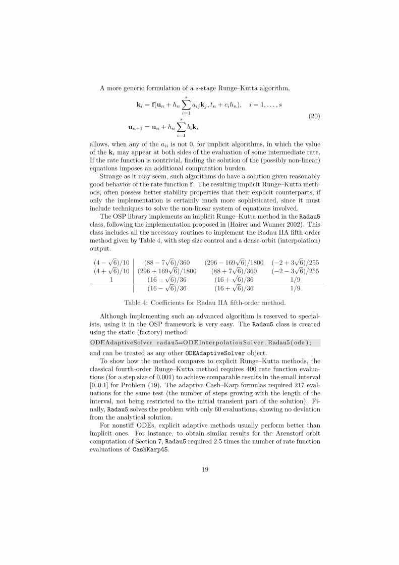
The OSP library implements an implicit Runge–Kutta method in the Radau5class, following the implementation proposed in (Hairer and Wanner 2002). Thisclass includes all the necessary routines to implement the Radau IIA fifth-ordermethod given by Table 4, with step size control and a dense-orbit (interpolation)output.

(4−√6)/10 (88− 7√

6)/360 (296− 169√

6)/1800 (−2 + 3√

6)/255(4 +

√6)/10 (296 + 169

√6)/1800 (88 + 7

√6)/360 (−2− 3

√6)/255

1 (16−√6)/36 (16 +√

6)/36 1/9(16−√6)/36 (16 +

√6)/36 1/9

Table 4: Coefficients for Radau IIA fifth-order method.

Although implementing such an advanced algorithm is reserved to special-ists, using it in the OSP framework is very easy. The Radau5 class is createdusing the static (factory) method:ODEAdaptiveSolver radau5=ODEInterpolat ionSolver . Radau5 ( ode ) ;

and can be treated as any other ODEAdaptiveSolver object.To show how the method compares to explicit Runge–Kutta methods, the

classical fourth-order Runge–Kutta method requires 400 rate function evalua-tions (for a step size of 0.001) to achieve comparable results in the small interval[0, 0.1] for Problem (19). The adaptive Cash–Karp formulas required 217 eval-uations for the same test (the number of steps growing with the length of theinterval, not being restricted to the initial transient part of the solution). Fi-nally, Radau5 solves the problem with only 60 evaluations, showing no deviationfrom the analytical solution.

For nonstiff ODEs, explicit adaptive methods usually perform better thanimplicit ones. For instance, to obtain similar results for the Arenstorf orbitcomputation of Section 7, Radau5 required 2.5 times the number of rate functionevaluations of CashKarp45.

19

Multistep methods. These methods take advantage of the information con-tained in previous steps of the solution. The general algorithm for a (p+1)-stepmethod is

un+1 =p∑

j=0

ajun−j + h

p∑

j=−1

bjfn−j , (n ≥ p) (21)

where fj represents f(uj , tj). Notice that, if b−1 6= 0, the method is implicit, andmust be solved by iteration. Simple multistep methods for initial value problemsbelong to two main families: Adams’ methods and backwards differentiationformulas.

Adams’ methods derive from numerical methods for the equivalent integralequation:

x(tn+1) = x(tn) +∫ tn+1

tn

f(x(t), t)dt. (22)

Typical examples of Adams’ method are the following fourth-order explicit andimplicit methods (Atkinson 1989):

un+1 = un +h

24(55fn − 59fn−1 + 37fn−2 − 9fn−3), (23a)

un+1 = un +h

24(9fn+1 + 19fn − 5fn−1 + fn−2). (23b)

Sometimes, explicit and implicit Adams formulas are applied in pairs, in predictor-corrector formulas. The latter is a mixed method that tries to obtain some ofthe stability properties of implicit formulas, with the simplicity of implementa-tion of explicit ones. The scheme uses first an explicit method to predict thesolution of the ODE at tn+1. It then corrects the approximation by applyingthe implicit formula with the value of fn+1 computed from the prediction.

Backwards differentiation formulas are obtained by approximating the solu-tion by a polynomial through a series of past un−j points and then taking un+1

such that the polynomial satisfies the ODE at tn+1. A typical result of thisprocess is (Hairer, Nørsett, and Wanner 2000):

2512

un+1 − 4un + 3un−1 − 43un−2 +

14un−3 = hfn+1. (24)

Both Adams’ methods and backwards differentiation formulas need the helpof an auxiliary method to start the process (that is, to compute the first p + 1points of the solution) and require that the steps be equally spaced. This re-quirement makes it complicated (though not impossible) to implement adaptivestep versions of the algorithms.

Extrapolation methods. These algorithms benefit from a particularly suit-able power expansion of the local error of some simple methods, to extrapolatebetween successive runs of the method with different step sizes, thus effectivelyaccelerating the convergence. The Bulirsch–Stoer method chooses a sequence of

20

increasing integer numbers N , and then uses, for each of them, a fixed step H,and h = H/N , the formula:

v1 = un + hf(un, tn) (25a)vi+1 = vi−1 + 2hf(vi, tn + ih), for i = 1, 2, · · · , N − 1 (25b)

un+1 =12

[vN + vN−1 + hf(vN , tn + H)] (25c)

to advance from (un, tn) to (un+1, tn + H). The error term for this formula isan expansion with only even powers of h. Standard extrapolation techniquescan then be used to obtain an arbitrarily high-order method that accuratelyapproximates the solution in the given interval (Press, Teukolsky, Vetterling,and Flannery 1992).

Symplectic integration methods. These methods can be the preferredchoice when studying Hamiltonian systems:

pi = −δH

δqi(p,q), qi =

δH

δpi(p,q), i = 1, . . . , k, (26)

which define a 2k-dimensional ODE with variables qi representing the general-ized coordinates of the system and pi the generalized momenta. Such problemsfrequently arise when modeling mechanical systems, where the Hamiltonian His the energy function of the system.

The symplectic property of these problems states that the flow of the systempreserves the differential 2-form:

ω2 =k∑

i=1

dpi ∧ dqi. (27)

If k = 1, the symplectic property has the geometrical interpretation that thearea (in phase space) is preserved by the flow.

When studying this type of system, a natural desire is that the numericalmethod used to solve the associated initial value problem also preserves thegeometric property. Such methods are called symplectic.

Although no explicit Runge–Kutta method is symplectic, it is possible to findhigh-order, so-called partitioned Runge–Kutta methods which are symplectic.These consist of a pair of Runge–Kutta methods with different sets of coefficientsapplied ‘separately’ to the variables pi and qi. For separable systems, in whichthe Hamiltonian is of the form H = T (p)+V (q), explicit such methods do exist(Hairer, Nørsett, and Wanner 2000; Enright, Higham, Owren, and Sharp 1995;Hairer, Lubich, and Wanner 2002).

A simple, lower-order symplectic method that can be applied to solving New-ton’s equation of motion a(t) = f(x(t), v(t), t) for a system of particles, is theVerlet algorithm. This is an easy to program, multistep method that producesstable long-term trajectories. The method has the additional advantage that,

21

although it does not preserve the energy of the system over short times, it doesproduce accurate averages over long times because the energy oscillates aboutthe mean. It therefore reduces the computational effort for systems where sta-tistical averages are more important than the accuracy of particular trajectories.

The partitioned Runge–Kutta coefficients for the Verlet method are given for(x, v) in Table 5. Because these coefficients define a simple implicit algorithm,it is convenient to solve for the values at tn+1. This reformulation, which isincluded in the OSP library, is known as the velocity form of the Verlet methodand is given by:

xn+1 = xn + vnh +12anh2 (28a)

vn+1 = vn +12(an+1 + an)h. (28b)

Important areas in which symplectic methods are preferred to other, perhapsmore accurate, methods, are molecular dynamics and astrophysics, where largescale simulations involving thousands of particles are studied over very long timescales (Gray, Noid, and Sumpter 1994).

0 0 01 1/2 1/2

1/2 1/2

1/2 1/2 01/2 1/2 0

1/2 1/2

Table 5: Partitioned Runge-Kutta coefficients for the Verlet method. The lefthand table is used to advance the position and the right table is used to advancethe velocity.

9 Events

Sometimes the model of a continuous system needs to include discontinuitiesin order to reflect special situations. The typical case is that of a collisionbetween two objects. Although the collision can be modeled at a microscopicscale, it is frequently much more convenient to stick to the macroscopic modeland instruct the computer to detect that the collision has taken place, find theprecise moment when it happened, compute explicitly the state of the systemafter the collision, and finally restart the continuous model from it. This is aparticular case of what is known as a state event.

Because our numerical method solves the ODE at given step sizes (eitherfixed or adaptive), a particular event will almost always take place in betweentwo successive computed states. A simple way to implement event detection isto provide a real valued function of the state, h(x), which changes sign wheneveran event takes place. The algorithm can then keep track of possible changesin the sign of h in each solution step and then apply a standard root-findingalgorithm to find the precise instant of time when the event takes place. The

22

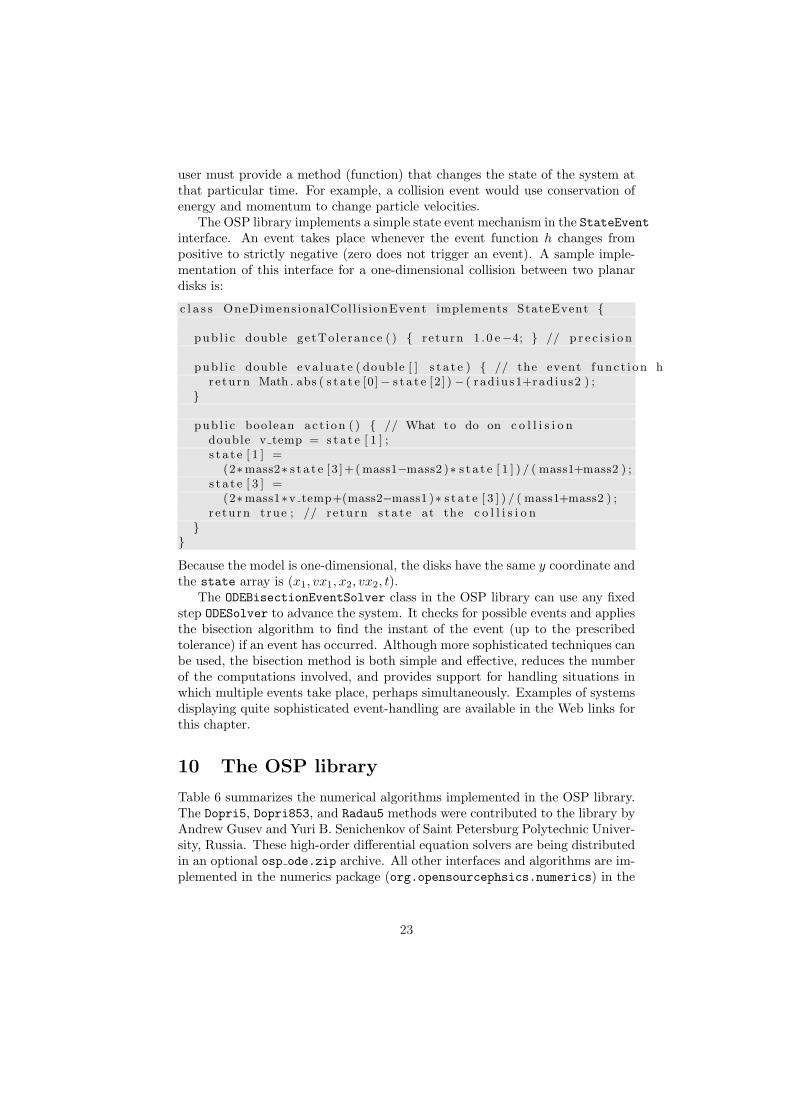
user must provide a method (function) that changes the state of the system atthat particular time. For example, a collision event would use conservation ofenergy and momentum to change particle velocities.

The OSP library implements a simple state event mechanism in the StateEventinterface. An event takes place whenever the event function h changes frompositive to strictly negative (zero does not trigger an event). A sample imple-mentation of this interface for a one-dimensional collision between two planardisks is:

c l a s s OneDimens ionalCol l i s ionEvent implements StateEvent {

pub l i c double getTolerance ( ) { re turn 1 .0 e−4; } // p r e c i s i o n

pub l i c double eva luate ( double [ ] s t a t e ) { // the event func t i on hreturn Math . abs ( s t a t e [0]− s t a t e [2 ] ) − ( rad ius1+rad ius2 ) ;

}

pub l i c boolean ac t i on ( ) { // What to do on c o l l i s i o ndouble v temp = s t a t e [ 1 ] ;s t a t e [ 1 ] =

(2∗mass2∗ s t a t e [ 3 ]+( mass1−mass2 )∗ s t a t e [ 1 ] ) / ( mass1+mass2 ) ;s t a t e [ 3 ] =

(2∗mass1∗v temp+(mass2−mass1 )∗ s t a t e [ 3 ] ) / ( mass1+mass2 ) ;r e turn true ; // re turn s t a t e at the c o l l i s i o n

}}Because the model is one-dimensional, the disks have the same y coordinate andthe state array is (x1, vx1, x2, vx2, t).

The ODEBisectionEventSolver class in the OSP library can use any fixedstep ODESolver to advance the system. It checks for possible events and appliesthe bisection algorithm to find the instant of the event (up to the prescribedtolerance) if an event has occurred. Although more sophisticated techniques canbe used, the bisection method is both simple and effective, reduces the numberof the computations involved, and provides support for handling situations inwhich multiple events take place, perhaps simultaneously. Examples of systemsdisplaying quite sophisticated event-handling are available in the Web links forthis chapter.

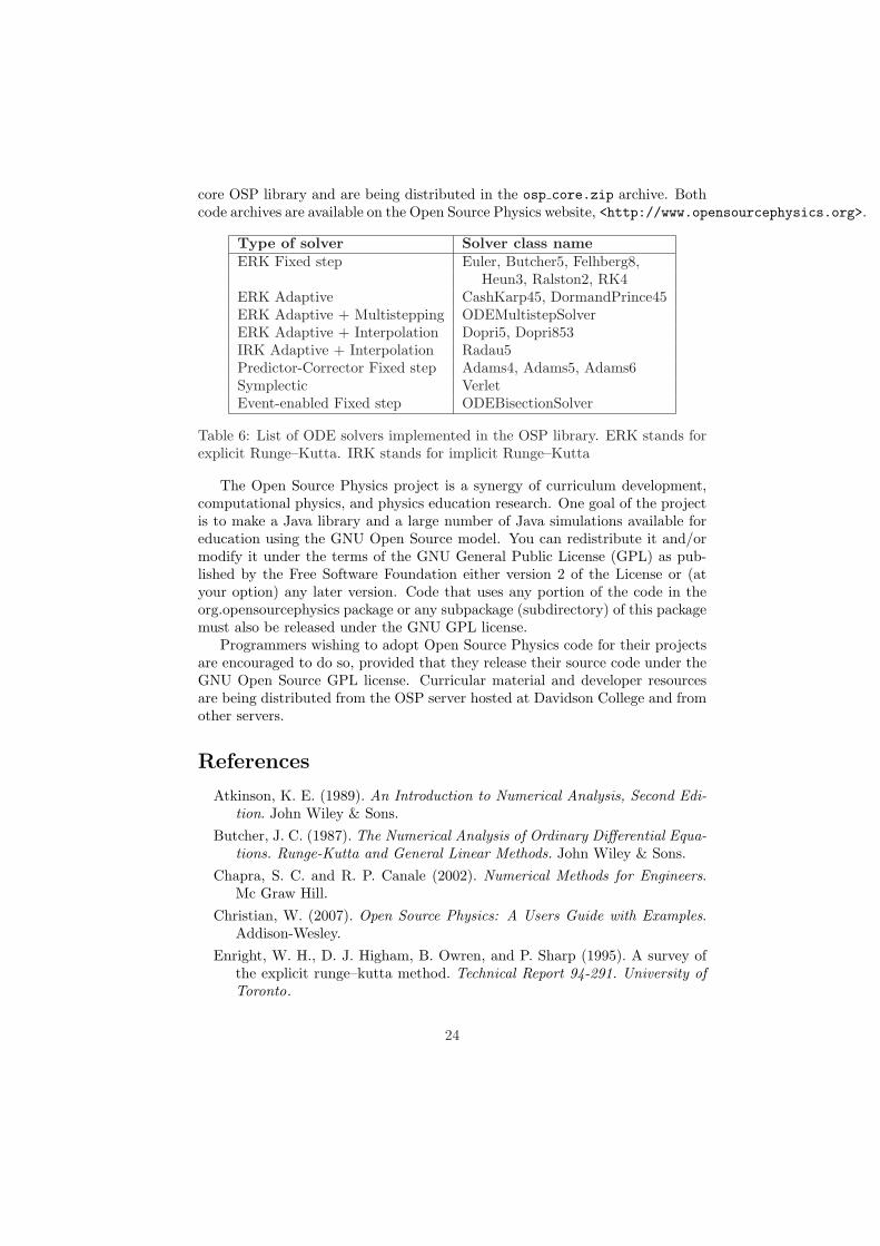
10 The OSP library

Table 6 summarizes the numerical algorithms implemented in the OSP library.The Dopri5, Dopri853, and Radau5 methods were contributed to the library byAndrew Gusev and Yuri B. Senichenkov of Saint Petersburg Polytechnic Univer-sity, Russia. These high-order differential equation solvers are being distributedin an optional osp ode.zip archive. All other interfaces and algorithms are im-plemented in the numerics package (org.opensourcephsics.numerics) in the

23

core OSP library and are being distributed in the osp core.zip archive. Bothcode archives are available on the Open Source Physics website, <http://www.opensourcephysics.org>.

Type of solver Solver class nameERK Fixed step Euler, Butcher5, Felhberg8,

Heun3, Ralston2, RK4ERK Adaptive CashKarp45, DormandPrince45ERK Adaptive + Multistepping ODEMultistepSolverERK Adaptive + Interpolation Dopri5, Dopri853IRK Adaptive + Interpolation Radau5Predictor-Corrector Fixed step Adams4, Adams5, Adams6Symplectic VerletEvent-enabled Fixed step ODEBisectionSolver

Table 6: List of ODE solvers implemented in the OSP library. ERK stands forexplicit Runge–Kutta. IRK stands for implicit Runge–Kutta

The Open Source Physics project is a synergy of curriculum development,computational physics, and physics education research. One goal of the projectis to make a Java library and a large number of Java simulations available foreducation using the GNU Open Source model. You can redistribute it and/ormodify it under the terms of the GNU General Public License (GPL) as pub-lished by the Free Software Foundation either version 2 of the License or (atyour option) any later version. Code that uses any portion of the code in theorg.opensourcephysics package or any subpackage (subdirectory) of this packagemust also be released under the GNU GPL license.

Programmers wishing to adopt Open Source Physics code for their projectsare encouraged to do so, provided that they release their source code under theGNU Open Source GPL license. Curricular material and developer resourcesare being distributed from the OSP server hosted at Davidson College and fromother servers.

References

Atkinson, K. E. (1989). An Introduction to Numerical Analysis, Second Edi-tion. John Wiley & Sons.

Butcher, J. C. (1987). The Numerical Analysis of Ordinary Differential Equa-tions. Runge-Kutta and General Linear Methods. John Wiley & Sons.

Chapra, S. C. and R. P. Canale (2002). Numerical Methods for Engineers.Mc Graw Hill.

Christian, W. (2007). Open Source Physics: A Users Guide with Examples.Addison-Wesley.

Enright, W. H., D. J. Higham, B. Owren, and P. Sharp (1995). A survey ofthe explicit runge–kutta method. Technical Report 94-291. University ofToronto.

24

Gray, S. K., D. W. Noid, and B. G. Sumpter (1994). Symplectic integratorsfor large scale molecular dynamics simulations: A comparison of severalexplicit methods. J. Chem. Phys. 101 (5) 4062–4072 .

Hairer, E., C. Lubich, and G. Wanner (2002). Geometric Numerical Inte-gration, Structure-Preserving Algorithms for Ordinary Differential Equa-tions. Springer.

Hairer, E., S. P. Nørsett, and G. Wanner (2000). Solving Ordinary DifferentialEquations I (Nonstiff Problems), 2nd Ed. Springer.

Hairer, E. and G. Wanner (2002). Solving Ordinary Differential Equations II(Stiff and Differential-Algenbaic Problems), 2nd Ed. Springer.

Keller, H. B. (1992). Numerical Methods For Two-Point Boundary-ValueProblems. Dover Publications, Inc.

Press, W. H., S. A. Teukolsky, W. T. Vetterling, and B. P. Flannery (1992).Numerical Recipes in C, The Art of Scientific Computing, 2nd Ed. Cam-bridge University Press.

Schilling, R. J. and S. L. Harris (2000). Applied Numerical Methods for En-gineers. Brooks/Cole.

25