Chapter 2

Numerical Methods for Stiff

Ordinary Differential

Equations

2.1 Stiff Ordinary Differential Equations

Remark 2.1 Stiffness. It was observed in Curtiss and Hirschfelder (1952) thatexplicit methods failed for the numerical solution of ordinary differential equationsthat model certain chemical reactions. They introduced the notation stiffness forsuch chemical reactions where the fastly reacting components arrive in a very shorttime in their equilibrium and the slowly changing components are more or lessfixed, i.e. stiff. In 1963, Dahlquist found out that the reason for the failure ofexplicit Runge–Kutta methods is their bad stability, see Section 2.5. It should beemphasized that the stability properties of the equations themselves are good, it isin fact a problem of the explicit methods.

There is no unique definition of stiffness in the literature. However, essentialproperties of stiff systems are as follows:

• There exist, for certain initial conditions, solutions that change slowly.• Solutions in a neighborhood of these smooth solutions converge quickly to them.

A definition of stiffness can be found in (Strehmel and Weiner, 1995, p. 202),(Strehmel et al., 2012, p. 208). This definition involves a certain norm that dependson the equation and it might be complicated to evaluate this norm. If the solution of(1.1) is sought in the interval [x0, xe] and if the right hand side of (1.1) is Lipschitzcontinous in the second argument with Lipschitz constant L, then an approximationof this definition is as follows. A system of ordinary differential equations is calledstiff if

L (xe − x0) � 1. (2.1)

Another definition of stiffness will be given in Definition 2.66. 2

Example 2.2 Stiff system of ordinary differential equations. Consider the system

y′1 = −80.6y1 + 119.4y2

y′2 = 79.6y1 − 120.4y2

in (0, 1). This is a linear system of ordinary differential equations that can bewritten in the form

y′ =

(−80.6 119.479.6 −120.4

)

y.

20

Taking as Lipschitz constant, e.g., the l1 norm of the system matrix (column sums),one gets L = 239.8 and condition (2.1) is satisfied. The general solution of thissystem is

y(x) = c1

(32

)

e−x + c2

(−11

)

e−200x.

It constants are determined by the initial condition. If the initial condition is suchthat c2 = 0, then the solution is smooth for all x > 0. Otherwise, if c2 6= 0, thenthe solutions changes rapidly for small x while approaching the smooth solution,see Figure 2.1 2

Figure 2.1: Solutions of Example 2.2, left: first component, right: second compo-nent.

2.2 Ordinary Differential Equations of Higher Or-

der

Remark 2.3 Motivation. The notation of stiffness comes from the considerationof first order systems of ordinary differential equations. There are some connectionsof such systems to ordinary differential equations of higher order, e.g. a solutionmethod for linear first order systems requires the solution of a higher order lineardifferential equation, see Remark 2.41. 2

2.2.1 Definition, Connection to First Order Systems

Definition 2.4 General and explicit n-th order ordinary differential equa-

tion. The general ordinary differential equation of order n has the form

F(

x, y(x), y′(x), . . . , y(n)(x))

= 0. (2.2)

This equation is called explicit, if one can write it in the form

y(n)(x) = f(

x, y(x), y′(x), . . . , y(n−1)(x))

. (2.3)

The function y(x) is a solution of (2.2) in an interval I if y(x) is n times continuouslydifferentiable in I and if y(x) satisfies (2.2).

Let x0 ∈ I be given. Then, (2.2) together with the conditions

y(x0) = y0, y′(x0) = y1, . . . , y(n−1)(x0) = yn−1

is called initial value problem for (2.2). 2

21

Example 2.5 Special cases. The general resp. explicit ordinary differential equa-tion of higher order can be solved analytically only in special cases. Two specialcases, that will not be considered here, are as follows:

• Consider the second order differential equation

y′′(x) = f(x, y′(x)).

Substituting y′(x) = z(x), one obtains a first order differential equation for z(x)

z′(x) = f(x, z(x)).

If one can solve this equation analytically, one gets y′(x). If it is then possibleto find a primitive of y′(x), one has computed an analytical solution of thedifferential equation of second order. In the case of an initial value problemwith

y(x0) = y0, y′(x0) = y1,

the initial value for the first order differential equation is

z(x0) = y1.

The second initial value is needed for determining the constant of the primitiveof y′(x).

• Consider the differential equation of second order

y′′(x) = f(y, y′).

Let a solution y(x) of this differential equation be known and let y−1(y) itsinverse function, i.e. y−1(y(x)) = x. Then, one can use the ansatz

p(y) := y′(y−1(y)

).

With the rule for differentiating the inverse function ((f−1)′(y0) = 1/f ′(x0)),one obtains

dp

dy(y) = y′′

(y−1(y)

) d

dy

(y−1(y(x))

)=

y′′(y−1(y)

)

y′(x)=

y′′(y−1(y)

)

y′ (y−1(y))

=y′′(y−1(y)

)

p(y)=

y′′(x)

p(y).

This approach leads then to the first order differential equation

p′(y) =f(y, p(y))

p(y).

2

Theorem 2.6 Connection of explicit ordinary differential equations of

higher order and systems of differential equations of first order. Everyexplicit differential equation of n-th order (2.3) can be transformed equivalently toa system of n differential equations of first order

y′k(x) = yk+1(x), k = 1, . . . , n− 1,

y′n(x) = f(x, y1(x), . . . , yn(x)) (2.4)

22

or (note that the system is generally nonlinear, since the unknown functions appearalso in f(·, . . . , ·))

y′(x) =

y′1(x)y′2(x)...

y′n(x)

=

0 1 0 · · · 00 0 1 · · · 0...

......

......

0 0 0 · · · 0

y1(x)y2(x)...

yn(x)

+

00...

f(x, y1, . . . , yn)

for the n functions y1(x), . . . , yn(x). The solution of (2.3) is y(x) = y1(x).

Proof: Insert in (2.3)

y1(x) := y(x), y2(x) := y′1(x) = y′(x), y3(x) := y′

2(x) = y′′(x), . . .

yn(x) := y′n−1(x) = y(n−1)(x).

If y ∈ Cn(I) is a solution of (2.3), then y1(x), . . . , yn(x) is obviously a solution of (2.4)in I.

Conversely, if y1(x), . . . , yn(x) ∈ C1(I) is a solution of (2.4), then it holds

y2(x) = y′1(x), y3(x) = y′

2(x) = y′′1 (x), . . . , yn(x) = y

(n−1)1 (x)

y′n(x) = y

(n)1 (x) = f(x, y1, . . . , yn).

Hence, the function y1(x) is n times continuously differentiable and it is the solution of

(2.3) in I.

Example 2.7 Transform of a higher order differential equation into a system offirst order equations. The third order differential equation

y′′′(x) + 2y′′(x)− 5y′(x) = f(x, y(x))

can be transformed into the form

y1(x) = y(x)

y′1(x) = y2(x)(= y′(x))

y′2(x) = y3(x)(= y′′(x))

y′3(x) = y′′′(x) = −2y′′(x) + 5y′(x) + f(x, y(x))

= −2y3(x) + 5y2(x) + f(x, y1(x)).

2

2.2.2 Linear Differential Equations of n-th Order

Definition 2.8 Linear n-th order differential equations. A linear differentialequation of n-th order has the form

an(x)y(n)(x) + an−1(x)y

(n−1)(x) + . . .+ a1(x)y′(x) + a0(x)y(x) = f(x), (2.5)

where the functions a0(x), . . . , an(x) are continuous in the interval I, in which asolution of (2.5) is searched, and it holds an(x) 6= 0 in I. The linear n-th orderdifferential equation is called homogeneous if f(x) = 0 for all x ∈ I

an(x)y(n)(x) + an−1(x)y

(n−1)(x) + . . .+ a1(x)y′(x) + a0(x)y(x) = 0. (2.6)

2

23

Theorem 2.9 Superposition principle for linear differential equations of

higher order. Consider the linear differential equation of n-th order (2.5), thenthe superposition principle holds:

i) If y1(x) and y2(x) are two solutions of the homogeneous equation (2.6), thenc1y1(x) + c2y2(x), c1, c2 ∈ R, is a solution of the homogeneous equation, too.

ii) If y0(x) is a solution of the inhomogeneous equation and y1(x) is a solution ofthe homogeneous equation, then y0(x)+y1(x) is a solution of the inhomogeneousequation.

iii) If y1(x) and y2(x) are two solutions of the inhomogeneous equation, then y1(x)−y2(x) is a solution of the homogeneous equation.

Proof: Direct calculations, exercise.

Cororllary 2.10 General solution of the inhomogeneous differential equa-

tion. The general solution of (2.5) is the sum of the general solution of the homo-geneous linear differential equation of n-th order (2.6) and one special solution ofthe inhomogeneous n-th order differential equation (2.5).

Remark 2.11 Transform in a linear system of ordinary differential equations offirst order. A linear differential equation of n-th order can be transformed equiva-lently into a linear n× n system

y′k(x) = yk+1(x), k = 1, . . . , n− 1,

y′n(x) = −n−1∑

i=0

ai(x)

an(x)yi+1(x) +

f(x)

an(x)

or

y′(x) =

y′1(x)y′2(x)

...y′n(x)

=

0 1 0 · · · 00 0 1 · · · 0...

......

......

− a0(x)an(x)

− a1(x)an(x)

− a2(x)an(x)

· · · −an−1(x)an(x)

y1(x)y2(x)

...yn(x)

+

00...

f(x)an(x)

=: A(x)y(x) + f(x). (2.7)

2

Theorem 2.12 Existence and uniqueness of a solution of the initial value

problem. Let I = [x0−a, x0+a] and ai ∈ C(I), i = 0, . . . , n, f ∈ C(I). Then, thelinear differential equation of n-th order (2.5) has exactly one solution y ∈ Cn(I)for given initial value

y(x0) = y0, y′(x0) = y1, . . . , y(n−1)(x0) = yn−1.

Proof: Since (2.5) is equivalent to the system (2.7), one can apply the theorem onglobal existence and uniqueness of a solution of an initial value problem from Picard–Lindelof, see lecture notes Numerical Mathematics I or the literature. To this end, one hasto show the Lipschitz continuity of the right-hand side of (2.7) with respect to y1, . . . , yn.Denoting the right-hand side by F (x,y) gives

‖F(x,y)− F(x, y)‖[C(I)]n = ‖A(y − y)‖[C(I)]n ≤ ‖A‖[C(I)]n,∞ ‖y − y‖[C(I)]n ,

24

where one uses the triangle inequality to get

‖Ai·y‖C(I) = maxx∈I

∣∣∣∣∣

n∑

j=1

aij(x)yj(x)

∣∣∣∣∣≤ max

x∈I

n∑

j=1

|aij(x)| maxj=1,...,n

{

maxx∈I

|yj(x)|

}

= ‖Ai·‖C(I) ‖y‖[C(I)]n

for i = 1, . . . , n. Now, one can choose

L = ‖A‖[C(I)]n,∞ = maxx∈I

{

max

{

1,

∣∣∣∣

a1(x)

an(x)

∣∣∣∣+ . . .+

∣∣∣∣

an−1(x)

an(x)

∣∣∣∣

}}

.

All terms are bounded since I is closed (compact) and continuous functions are bounded

on compact sets.

Definition 2.13 Linearly independent solutions, fundamental system. Thesolutions yi(x) : I → R, i = 1, . . . , k, of (2.6) are called linearly independent iffrom

k∑

i=1

ciyi(x) = 0, for all x ∈ I, ci ∈ R,

it follows that ci = 0 for i = 1, . . . , k. A set of n linearly independent solutions iscalled a fundamental system of (2.6). 2

Definition 2.14 Wronski1 matrix, Wronski determinant. Let yi(x), i =1, . . . , k, be solutions of (2.6). The matrix

W(x) =

y1(x) . . . yk(x)y′1(x) . . . y′k(x)

...

y(n−1)1 (x) . . . y

(n−1)k (x)

is called Wronski matrix. For k = n the Wronski determinant is given bydet(W)(x) =: W (x). 2

Lemma 2.15 Properties of the Wronski matrix and Wronski determi-

nant. Let I = [a, b] and let y1(x), . . . , yn(x) be solutions of (2.6).

i) The Wronski determinant fulfills the linear first order differential equation

W ′(x) = −an−1(x)

an(x)W (x).

ii) It holds for all x ∈ I

W (x) = W (x0) exp

(

−∫ x

x0

an−1(t)

an(t)dt

)

with arbitrary x0 ∈ I.iii) If there exists a x0 ∈ I with W (x0) 6= 0, then it holds W (x) 6= 0 for all x ∈ I.iv) If there exists a x0 ∈ I with rank(W(x0)) = k, then there are at least k solutions

of (2.6), e.g. y1(x), . . . , yk(x), linearly independent.

Proof:

1Joseph Marie Wronski (1758 – 1853)

25

i) Let Sn be the set of all permutations of {1, . . . , n} and let σ ∈ Sn. Denote the entriesof the Wronski matrix by W(x) = (yjk(x))

n

j,k=1. If σ = (σ1, . . . , σn), then let

n∏

j=1

yj,σj(x) = (y1,σ1

y2,σ2. . . yn,σn) (x).

Applying the Laplace2 formula for determinants and the product rule yields

d

dxdet(W(x)) =

d

dx

(∑

σ∈Sn

(

sgn(σ)

n∏

j=1

yj,σj(x)

))

=∑

σ∈Sn

sgn(σ)

n∑

i=1

n∏

j=1,j 6=i

yj,σj(x)

y′i,σi

(x)

=

n∑

i=1

∑

σ∈Sn

sgn(σ)

n∏

j=1,j 6=i

yj,σj(x)y′

i,σi(x)

=

n∑

i=1

det

· · · · · · · · ·(

y(i−1)1 (x)

)′

· · ·(

y(i−1)n (x)

)′

· · · · · · · · ·

.

exercise for n = 2, 3. In the last step, again the Laplace formula for determinants wasapplied. In the i-th row of the last matrix is the first derivative of the correspondingrow of the Wronski matrix, i.e. there is the i-th order derivative of (y1(x), . . . , yn(x)).The rows with dots in this matrix coincide with the respective rows of W(x). Fori = 1, . . . , n − 1, the determinants vanish, since in these cases there are two identicalrows, namely row i and i+ 1. Thus, it is

d

dxdet(W(x)) = det

y1(x) . . . yn(x)y′1(x) . . . y′

n(x)...

y(n−2)1 (x) . . . y

(n−2)n (x)

y(n)1 (x) . . . y

(n)n (x)

.

Now, one uses that y1(x), . . . , yn(x) are solutions of (2.6) and one replaces the n-thderivative in the last row by (2.6). Using rules for the evaluation of determinants, oneobtains

d

dxdet(W(x)) =

n∑

i=1

−ai−1(x)

an(x)det

y1(x) . . . yn(x)y′1(x) . . . y′

n(x)...

y(i−1)1 (x) . . . y

(i−1)n (x)

.

Apart of the last term, all other determinants vanish, since all other terms have twoidentical rows, namely the i-th row and the last row.

ii) This term is the solution of the initial value problem for the Wronski determinant andthe initial value W (x0), see the respective theorem in the lecture notes of NumericalMathematics I.

iii) This statement follows directly from ii) since the exponential does not vanish.

iv) exercise

Theorem 2.16 Existence of a fundamental system, representation of the

solution of a homogeneous linear differential equation of n-th order by

the fundamental system. Let I = [a, b] with x0 ∈ I. The homogeneous equation(2.6) has a fundamental system in I. Each solution of (2.6) can be written as alinear combination of the solutions of an arbitrary fundamental system.

2Pierre–Simon (Marquis de) Laplace (1749 – 1827)

26

Proof: Consider n homogeneous initial value problems with the initial values

y(i−1)j (x0) = δij , i, j = 1, . . . , n.

Each of these initial value problems has a unique solution yj(x), see Theorem 2.12. It isW (x0) = 1 for these solutions. From Lemma 2.15, iii), it follows that {y1(x), . . . , yn(x)}is a fundamental system.

Let y(x) be an arbitrary solution of (2.6) with the initial values y(i−1)(x0) = yi−1,i = 1, . . . , n, and {y1(x), . . . , yn(x)} an arbitrary fundamental system. The system

y1(x0) . . . yn(x0)y′1(x0) . . . y′

n(x0)...

y(n−1)1 (x0) . . . y

(n−1)n (x0)

c0c1...

cn−1

=

y0y1...

yn−1

has a unique solution since the matrix spanned by a fundamental system is not singular.

The function∑n

i=1 ci−1yi(x) satisfies the initial conditions (these are just the equations

of the system) and, because of the superposition principle, it is a solution of (2.6). Since

the solution of the initial value problem to (2.6) is unique, Theorem 2.12, it follows that

y(x) =∑n

i=1 ci−1yi(x).

Theorem 2.17 Special solution of the inhomogeneous equation. Let{y1(x), . . . , yn(x)} be a fundamental system of the homogeneous equation (2.6) inI = [a, b]. In addition, let Wl(x) be the determinant, which is obtained from theWronski determinant W (x) with respect to {y1(x), . . . , yn(x)} by replacing the l-thcolumn by (0, 0, . . . , f(x)/an(x))

T . Then,

y(x) =n∑

l=1

yl(x)

∫ x

x0

Wl(t)

W (t)dt, x0, x ∈ I,

is a solution of the inhomogeneous equation (2.5).

Proof: The proof uses the principle of the variation of the constants. This principle

will be explained in a simpler setting in Remark 2.29. For details of the proof, see the

literature.

2.2.3 Linear n-th Order Differential Equations with Constant

Coefficients

Definition 2.18 Linear differential equation of n-th order with constant

coefficients. A linear n-th order differential equation with constant coefficientshas the form

any(n)(x) + an−1y

(n−1)(x) + . . .+ a1y′(x) + a0y(x) = f(x), (2.8)

with ai ∈ R, i = 0, . . . , n, an 6= 0. 2

The Homogeneous Equation

Remark 2.19 Basic approach for solving the homogeneous linear differential equa-tion of n-th order with constant coefficients. Because of the superposition princi-ple, one needs the general solution of the homogeneous differential equation. Thatmeans, one has to find a fundamental system, i.e. n linearly independent solutions.

Considern∑

i=0

aiy(i)h (x) = 0. (2.9)

27

In the case of a differential equation of first order, i.e. n = 1,

a1y′h(x) + a0yh(x) = 0,

one can get the solution by the method of separating the variables (unknowns), seelecture notes of Numerical Mathematics I. One obtains

yh(x) = c exp

(

−a0a1

x

)

, c ∈ R.

One uses the same structural ansatz for computing the solution of (2.9)

yh(x) = eλx, λ ∈ C. (2.10)

It follows thaty′h(x) = λeλx, . . . , y

(n)h (x) = λneλx.

Inserting into (2.9) gives

(anλ

n + an−1λn−1 + . . .+ a1λ+ a0

)eλx = 0. (2.11)

It is eλx 6= 0, also for complex λ. Because, using Euler’s formula, it holds forλ = a+ ib, a, b ∈ R, that

eλx = eax (cos(bx) + i sin(bx)) = eax cos(bx) + ieax sin(bx).

A complex number is zero iff its real part and its imaginary part are vanish. It iseax > 0 and there does not exist a (bx) ∈ R such that at the same time sin(bx) andcos(bx) vanish. Hence, eλx 6= 0.

The equation (2.11) is satisfied iff one of the factors is equal to zero. Since thesecond factor cannot vanish, it must hold

p(λ) := anλn + an−1λ

n−1 + . . .+ a1λ+ a0 = 0.

The function p(λ) is called characteristic polynomial of (2.9). The roots of thecharacteristic polynomial are the values of λ in the ansatz of yh(x).

From the fundamental theorem of algebra it holds that p(λ) has exactly n roots,which do not need to be mutually different. Since the coefficients of p(λ) are realnumbers, it follows that with each complex root λ1 = a + ib, a, b ∈ R, b 6= 0, alsoits conjugate λ2 = a− ib is a root of p(λ).

It will be shown that the basic ansatz (2.10) is not sufficient in the case ofmultiple roots. 2

Theorem 2.20 Linearly independent solutions in the case of real roots

with multiplicity k. Let λ0 ∈ R be a real root of the characteristic polynomialp(λ) with multiplicity k, 1 ≤ k ≤ n. Then, one can obtain with λ0 the k linearlyindependent solutions of (2.9)

yh,1(x) = eλ0x, yh,2(x) = xeλ0x, . . . , yh,k(x) = xk−1eλ0x. (2.12)

Proof: For k = 2.yh,1(x), yh,2(x) solve (2.9). This statement is already clear for yh,1(x) since this func-

tion has the form of the ansatz (2.10). For yh,2(x) it holds

y′h,2(x) = (1 + λ0x) e

λ0x,

y′′h,2(x) =

(2λ0 + λ2

0x)eλ0x,

...

y(n)h,2(x) =

(nλn−1

0 + λn0x)eλ0x.

28

Inserting into the left-hand side of (2.9) yields

eλ0x

n∑

i=0

ai(iλi−10 + λi

0x) = eλ0x

(

x

n∑

i=0

aiλi0

︸ ︷︷ ︸

p(λ0)

+

n∑

i=0

aiiλi0

︸ ︷︷ ︸

p′(λ0)

)

. (2.13)

It is p(λ0) = 0, since λ0 is a root of p(λ). The second term is the derivative p′(λ) of p(λ)at λ0. Since the multiplicity of λ0 is two, one can write p(λ) in the form

p(λ) = (λ− λ0)2 p0(λ),

where p0(λ) is a polynomial of degree n− 2. It follows that

p′(λ) = 2 (λ− λ0) p0(λ) + (λ− λ0)2 p′0(λ).

Hence, it holds p′(λ0) = 0, (2.13) vanishes, and yh,2(x) is a solution of (2.9).yh,1(x), yh,2(x) are linearly independent. One has to show, Lemma 2.15, that the

Wronski determinant does not vanish. It holds

W (x) = det

(yh,1(x) yh,2(x)y′h,1(x) y′

h,2(x)

)

= det

(eλ0x xeλ0x

λ0eλ0x (1 + λ0x)e

λ0x

)

= e2λ0x det

(1 xλ0 1 + λ0x

)

= e2λ0x (1 + λ0x− λ0x) = e2λ0x > 0

for all x ∈ I.

Roots of multiplicity k > 2. The principle proof is analogous to the case k = 2,

where one uses the factorization p(λ) = (λ− λ0)k p0(λ). The computation of the Wronski

determinant becomes more involved.

Remark 2.21 Complex roots. The statement of Theorem 2.20 is true also forcomplex roots of p(λ). The Wronski determinant is e2λ1x 6= 0. However, thecorresponding solutions, e.g.

y1,h(x) = eλ1x = e(a+ib)x

are complex-valued. Since one has real coefficients in (2.9), one likes to obtain alsoreal-valued solutions. Such solutions can be constructed from the complex-valuedsolutions.

Let λ1 = a + ib, λ1 = a − ib, a, b ∈ R, b 6= 0, be a conjugate complex roots ofp(λ), then one obtains with Euler’s formula

eλ1x = e(a+ib)x = eax (cos(bx) + i sin(bx)) ,

eλ1x = e(a−ib)x = eax (cos(bx)− i sin(bx)) .

Because of the superposition principle, each linear combination is also solution of(2.9). 2

Theorem 2.22 Linearly independent solution for simple conjugate com-

plex roots. Let λ1 ∈ C, λ1 = a+ ib, b 6= 0, be a simple conjugate complex root ofthe characteristic polynomial p(λ) with real coefficients. Then,

yh,1(x) = Re(eλ1x

)= eax cos(bx), yh,2(x) = Im

(eλ1x

)= eax sin(bx),

are real-valued, linearly independent solutions of (2.9).

Proof: Use the superposition principle for proving that the functions are solutions

and the Wronski determinant for proving that they are linearly independent, exercise.

29

Theorem 2.23 Linearly independent solution for conjugate complex roots

with multiplicity greater than one. Let λ1 ∈ C, λ1 = a+ ib, b 6= 0, be a conju-gate complex root with multiplicity k of the characteristic polynomial p(λ) with realcoefficients. Then,

yh,1(x) = eax cos(bx), . . . , yh,k(x) = xk−1eax cos(bx),

yh,k+1(x) = eax sin(bx), . . . , yh,2k(x) = xk−1eax sin(bx) (2.14)

are real-valued, linearly independent solutions of (2.9).

Proof: The proof is similarly to the previous theorems.

Theorem 2.24 Fundamental system for (2.9). Let p(λ) be the characteristicpolynomial of (2.9) with the roots λ1, . . . , λn ∈ C, where the roots are counted incorrespondence to their multiplicity. Then, the set of solutions of form (2.12) and(2.14) form a fundamental system of (2.9).

Proof: A real root with multiplicity k gives k linearly independent solutions and aconjugate complex root with multiplicity k gives 2k linearly independent solutions. Thus,the total number of solutions of form (2.12) and (2.14) is equal to the number of roots ofp(λ). This number is equal to n, because of the fundamental theorem of algebra. It isknown from Theorem 2.16 that a fundamental system has exactly n functions. Altogether,the correct number of functions is there.

One can show that solutions that correspond to different roots are linearly independent,

e.g., (Gunther et al., 1974, p. 75). The linearly independence of the solutions that belong

to the same root, was already proved.

Example 2.25 Homogeneous second order linear differential equation with con-stant coefficients.

1. Considery′′(x) + 6y′(x) + 9y(x) = 0.

The characteristic polynomial is

p(λ) = λ2 + 6λ+ 9

with the roots λ1 = λ2 = −3. One obtains the fundamental system

yh,1(x) = e−3x, yh,2(x) = xe−3x.

The general solution of the homogeneous equation has the form

yh(x) = c1yh,1(x) + c2yh,2(x) = c1e−3x + c2xe

−3x, c1, c2 ∈ R.

2. Consider

y′′(x) + 4y(x) = 0 =⇒ p(λ) = λ2 + 4 =⇒ λ1,2 = ±2i.

It follows that

yh,1(x) = cos(2x), yh,2(x) = sin(2x)

yh(x) = c1 cos(2x) + c2 sin(2x), c1, c2 ∈ R.

2

30

The Inhomogeneous Equation

Remark 2.26 Goal. Because of the superposition principle, a special solution of(2.8) has to be found. This section sketches several possibilities to obtain such asolution. 2

Remark 2.27 Appropriate ansatz (Storgliedansatze). If the right-hand side f(x)possesses a special form, it is possible to obtain a solution of the inhomogeneousequation (2.8) with an appropriate ansatz. From (2.8) it becomes clear, that thisway works only if on the left-hand side and the right-hand side of the equation arethe same types of functions. In particular, one needs the same types of functions foryi(x) and all derivatives up to order n. This approach works, e.g., for the followingclasses of right-hand sides:

• f(x) is a polynomial

f(x) = b0 + b1x+ . . .+ bmxm, bm 6= 0.

The appropriate ansatz is also a polynomial

yi(x) = xk (c0 + c1x+ . . .+ cmxm) ,

where 0 is a root of p(λ) with multiplicity k.• If the right-hand side is

f(x) = (b0 + b1x+ . . .+ bmxm) eax,

then one can use the following ansatz

yi(x) = xk (c0 + c1x+ . . .+ cmxm) eax,

where a is a root of p(λ) with multiplicity k. The first class of functions is justa special case for a = 0.

• For right-hand sides of the form

f(x) = (b0 + b1x+ . . .+ bmxm) cos(bx),

f(x) = (b0 + b1x+ . . .+ bmxm) sin(bx),

one can use the ansatz

yi(x) = xk (c0 + c1x+ . . .+ cmxm) cos(bx)

+xk (d0 + d1x+ . . .+ dmxm) sin(bx),

if ib is a root of p(λ) with multiplicity k.

One can find the ansatz for more right-hand sides in the literature, e.g. in Heuser(2006). 2

Example 2.28 Appropriate ansatz (Storgliedansatz). Consider

y′′(x)− y′(x) + 2y(x) = cosx.

The appropriate ansatz is given by

yi(x) = a cosx+ b sinx =⇒y′i(x) = −a sinx+ b cosx =⇒y′′i (x) = −a cosx− b sinx.

31

Inserting into the equation gives

−a cosx− b sinx+ a sinx− b cosx+ 2a cosx+ 2b sinx = cosx =⇒(−a− b+ 2a) cosx+ (−b+ a+ 2b) sinx = cosx.

The last equation is satisfied if the numbers a, b solve the following linear system ofequations

a− b = 1, a+ b = 0 =⇒ a =1

2, b = −1

2.

One obtains the special solution

yi(x) =1

2(cosx− sinx) .

2

Remark 2.29 Variation of the constants. If one cannot find an appropriate ansatz,then one can try the variation of the constants. This approach will be demonstratedfor the second order differential equation

y′′(x) + a1y′(x) + a0y(x) = f(x). (2.15)

Let yh,1(x), yh,2(x) be two linearly independent solutions of the homogeneous dif-ferential equation such that

yh(x) = c1yh,1(x) + c2yh,2(x)

is the general solution of the homogeneous equation. Now, one makes the ansatz

yi(x) = c1(x)yh,1(x) + c2(x)yh,2(x)

with two unknown functions c1(x), c2(x). The determination of these functionsrequires two conditions. One has

y′i(x) = c′1(x)yh,1(x) + c1(x)y′h,1(x) + c′2(x)yh,2(x) + c2(x)y

′h,2(x)

= (c′1(x)yh,1(x) + c′2(x)yh,2(x)) + c1(x)y′h,1(x) + c2(x)y

′h,2(x).

Now, one sets the term in the parentheses zero. This is the first condition. It followsthat

y′′i (x) = c′1(x)y′h,1(x) + c1(x)y

′′h,1(x) + c′2(x)y

′h,2(x) + c2(x)y

′′h,2(x).

Inserting this expression into (2.15) gives

f(x) = c′1(x)y′h,1(x) + c1(x)y

′′h,1(x) + c′2(x)y

′h,2(x) + c2(x)y

′′h,2(x)

+a1(c1(x)y

′h,1(x) + c2(x)y

′h,2(x)

)+ a0 (c1(x)yh,1(x) + c2(x)yh,2(x))

= c1(x)(y′′h,1(x) + a1y

′h,1(x) + a0yh,1(x)

)

︸ ︷︷ ︸

=0

+c2(x)(y′′h,2(x) + a1y

′h,2(x) + a0yh,2(x)

)

︸ ︷︷ ︸

=0

+c′1(x)y′h,1(x) + c′2(x)y

′h,2(x).

This is the second condition. Summarizing both conditions gives the followingsystem of equations

(yh,1(x) yh,2(x)y′h,1(x) y′h,2(x)

)(c′1(x)c′2(x)

)

=

(0

f(x)

)

.

32

This system possesses a unique solution since yh,1(x), yh,2(x) are linearly indepen-dent from what follows that the determinant of the system matrix, which is justthe Wronksi matrix, is not equal to zero. The solution is

c′1(x) = − f(x)yh,2(x)

yh,1(x)y′h,2(x)− y′h,1(x)yh,2(x), c′2(x) =

f(x)yh,1(x)

yh,1(x)y′h,2(x)− y′h,1(x)yh,2(x).

The success of the method of the variation of the constants depends only on thedifficulty to find the primitives of c′1(x) and c′2(x).

For equations of order higher than two, one has the goal to get a linear systemof equations for c′1(x), . . . , c

′n(x). To this end, one sets for each derivative of the

ansatz the terms with c′1(x), . . . , c′n(x) equal to zero. The obtained linear system of

equations has as matrix the Wronski matrix and as right-hand side a vector, whosefirst (n− 1) components are equal to zero and whose last component is f(x). 2

Example 2.30 Variation of the constants. Find the general solution of

y′′(x) + 6y′(x) + 9y(x) =e−3x

1 + x.

The general solution of the homogeneous equation is

yh(x) = c1e−3x + c2xe

−3x,

see Example 2.25. The variation of the constants leads to the following system oflinear equations

(e−3x xe−3x

−3e−3x (1− 3x)e−3x

)(c′1(x)c′2(x)

)

=

(0

e−3x

1+x

)

.

Using, e.g., the Cramer rule, gives

c′1(x) = −e−6x

(x

1+x

)

(1− 3x+ 3x)e−6x= − x

1 + x,

c′2(x) =e−6x

(1

1+x

)

(1− 3x+ 3x)e−6x=

1

1 + x.

One obtains

c1(x) = −∫

x

1 + xdx = −

∫1 + x

1 + xdx+

∫1

1 + xdx = −x+ ln |1 + x| ,

c2(x) =

∫1

1 + xdx = ln |1 + x| .

Thus, one gets

yi(x) = (−x+ ln |1 + x|) e−3x + ln |1 + x|xe−3x

and one obtains for the general solution

y(x) = (−x+ ln |1 + x|+ c1) e−3x + (ln |1 + x|+ c2)xe

−3x.

Inserting this function into the equation proves the correctness of the result. 2

33

2.3 Linear Systems of Ordinary Differential Equa-

tions of First Order

2.3.1 Definition, Existence and Uniqueness of a Solution

Definition 2.31 Linear system of first order differential equations. In a lin-ear system of ordinary differential equations of first order one tries to find functionsy1(x), . . . , yn(x) : I → R, I = [a, b] ⊂ R, that satisfy the system

y′i(x) =n∑

j=1

aij(x)yj(x) + fi(x), i = 1, . . . , n,

or in matrix-vector notation

y′(x) = A(x)y(x) + f(x) (2.16)

with

y(x) =

y1(x)...

yn(x)

, y′(x) =

y′1(x)...

y′n(x)

,

A(x) =

a11(x) · · · a1n(x)...

. . ....

an1(x) · · · ann(x)

, f(x) =

f1(x)...

fn(x)

,

where aij(x), fi(x) ∈ C(I). If f(x) ≡ 0, then the system is called homogeneous. 2

Theorem 2.32 Superposition principle for linear systems. Consider the lin-ear system of ordinary differential equations (2.16), then the superposition principleholds:

i) If y1(x) and y2(x) are two solutions of the homogeneous systems, then c1y1(x)+c2y2(x), c1, c2 ∈ R, is a solution of the homogeneous system, too.

ii) If y0(x) is a solution of the inhomogeneous system and y1(x) is a solution ofthe homogeneous system, then y0(x)+y1(x) is a solution of the inhomogeneoussystem.

iii) If y1(x) and y2(x) are two solutions of the inhomogeneous system, then y1(x)−y2(x) is a solution of the homogeneous system.

Proof: Direct calculations, exercise.

Cororllary 2.33 General solution of the inhomogeneous system.

i) If y1(x),y2(x), . . . ,yk(x) are solutions of the homogeneous system, then any

linear combination∑k

i=1 ciyi(x), c1, . . . , ck ∈ R, is also a solution of the homo-geneous system.

ii) The general solution of the inhomogeneous system is the sum of a special solu-tion of the inhomogeneous system and the general solution of the homogeneoussystem.

Theorem 2.34 Existence and uniqueness of a solution of the initial value

problem. Let I = [x0−a, x0+a] and aij ∈ C(I), fi ∈ C(I), i, j = 1, . . . , n. Then,there is exactly one solution y(x) : I → R

n of the initial value problem to (2.16)with the initial value y(x0) = y0 ∈ R

n.

34

Proof: The statement of the theorem follows from the theorem on global existenceand uniqueness of a solution of an initial value problem from Picard–Lindelof, see lecturenotes Numerical Mathematics I or the literature.

Since the functions aij(x) are continuous on the closed (compact) interval I, they arealso bounded due to the Weierstrass theorem. That means, there is a constant M with

|aij(x)| ≤ M, x ∈ I, i, j = 1, . . . , n.

Denoting the right hand side of (2.16) by f(x,y), it follows that

‖f(x,y1)− f(x,y2)‖∞ = maxi=1,...,n

|fi(x,y1)− fi(x,y2)|

= maxi=1,...,n

∣∣∣∣∣

n∑

j=1

aij(x)y1,j(x) + fi(x)−

n∑

j=1

aij(x)y2,j(x)− fi(x)

∣∣∣∣∣

= maxi=1,...,n

∣∣∣∣∣

n∑

j=1

aij(x) (y1,j(x)− y2,j(x))

∣∣∣∣∣

≤ n maxi,j=1,...,n

|aij(x)| maxi=1,...,n

|y1,i(x)− y2,i(x)|

≤ nM ‖y1 − y2‖∞ ,

i.e. the right hand side satisfies a uniform Lipschitz condition with respect to y with the

Lipschitz constant nM . Hence, the assumptions of the theorem on global existence and

uniqueness of a solution of an initial value problem from Picard–Lindelof are satisfied.

2.3.2 Solution of the Homogeneous System

Remark 2.35 Scalar case. Because of the superposition principle, one needs thegeneral solution of the homogeneous system

y′(x) = A(x)y(x) (2.17)

for finding the general solution of (2.16). The homogeneous system has always thetrivial solution y(x) = 0.

In the scalar case y′(x) = a(x)y(x), the general solution has the form

y(x) = c exp

(∫ x

x0

a(t) dt

)

, c ∈ R, x0 ∈ (a, b),

see lecture notes Numerical Mathematics I or the literature. Also for the system(2.17), it is possible to specify the general solution with the help of the exponential.

2

Definition 2.36 Matrix exponential. Let A ∈ Rn×n and

A0 := I, A1 := A, A2 := AA, . . . , Ak := Ak−1A.

The matrix exponential is defined by

eA := exp(A) : Rn×n → R

n×n, A 7→∞∑

k=0

Ak

k!.

2

Lemma 2.37 Properties of the matrix exponential. The matrix exponentialhas the following properties:

35

i) The series∞∑

k=0

Ak

k!

converges absolutely for all A ∈ Rn×n, like in the real case n = 1.

ii) If the matrices A,B ∈ Rn×n are commuting, i.e., if AB = BA holds, then it

follows thateAeB = eA+B .

iii) The matrix(eA)−1 ∈ R

n×n exists for all A ∈ Rn×n and it holds

(eA)−1

= e−A.

This property corresponds to ex 6= 0 for the scalar case.iv) It holds rank

(eA)= n, det

(eA)6= 0.

v) The matrix-valued function R → Rn×n, x 7→ eAx, where Ax is defined component-

wise, is continuously differentiable with respect to x with

d

dxeAx = AeAx.

The derivative of the exponential is the first factor in this matrix product. Theformula looks the same as in the real case.

Proof:

i) with induction and comparison test with a majorizing series, see literature,

ii) follows from i), exercise,

iii) follows from ii), exercise,

iv) follows from iii),

v) direct calculation with difference quotient, exercise.

Example 2.38 Matrix exponential. There are only few classes of matrices that al-low an easy computation of the matrix exponential: diagonal matrices and nilpotentmatrices.

1. Consider

A =

1 0 00 2 00 0 3

=⇒ Ak =

1k 0 00 2k 00 0 3k

.

It follows that

eAx =∞∑

k=0

(Ax)k

k!=

∞∑

k=0

1

k!

xk 0 00 (2x)k 00 0 (3x)k

=

∑∞k=0

xk

k! 0 0

0∑∞

k=0(2x)k

k! 0

0 0∑∞

k=0(3x)k

k!

=

ex 0 00 e2x 00 0 e3x

.

2. This example illustrates property ii) of Lemma 2.37. For the matrices

A =

(2 00 3

)

, B =

(0 10 0

)

,

36

it is possible to calculate the corresponding series easily, since B is a nilpotentmatrix (B2 = 0). One obtains

eA =

(e2 00 e3

)

, eB =

(1 10 1

)

.

It holds that

eAeB =

(e2 e2

0 e3

)

6=(

e2 e3

0 e3

)

= eBeA.

2

Theorem 2.39 General solution of the homogeneous linear system of first

order. The general solution of (2.17) is

yh(x) = e∫

x

x0A(t) dt

c, c ∈ Rn, x0 ∈ (a, b). (2.18)

The integral is defined component-wise.

Proof: i) (2.18) is a solution of (2.17). This statement follows from the derivativeof the matrix exponential and the rule on the differentiation of an integral with respect tothe upper limit

y′h(x) =

d

dx

(

e∫xx0

A(t) dtc)

=d

dx

(∫ x

x0

A(t) dt

)

e∫xx0

A(t) dtc = A(x)e

∫xx0

A(t) dtc.

ii) every solution of (2.17) is of form (2.18). Consider an arbitrary solution yh(x) of(2.17) with yh(x0) ∈ R

n. Take in (2.18) c = yh(x0). Then, it follows that

yh(x0) = e∫x0x0

A(t) dtyh(x0) = e0

︸︷︷︸

=I

yh(x0) = yh(x0).

That means, e∫xx0

A(t) dtyh(x0) is a solution of (2.17) which has in x0 the same initial value

as yh(x). Since the solution of the initial value problem is unique, Theorem 2.34, it follows

that yh(x) = e∫xx0

A(t) dtyh(x0).

2.3.3 Linear Systems of First Order with Constant Coeffi-

cients

Remark 2.40 Linear system of first order differential equations with constant co-efficients. A linear system of first order differential equations with constant coeffi-cients has the form

y′(x) = Ay(x) + f(x), A =

a11 · · · a1n...

. . ....

an1 · · · ann

∈ R

n×n. (2.19)

Thus, the homogeneous system has the form

y′(x) = Ay(x). (2.20)

Its general solution is given by

yh(x) = eAxc, c ∈ Rn, (2.21)

see Theorem 2.39. 2

37

Remark 2.41 Elimination method, substitution method for the homogeneous sys-tem. One needs, due to the superposition principle, the general solution of thehomogeneous system. In practice, it is generally hard to compute exp(Ax) be-cause it is defined by an infinity series. For small systems, i.e. n ≤ 3, 4, one canuse the elimination or substitution method for computing the general solution of(2.20). This method is already known from the numerical solution of linear systemsof equations. One solves one equation for a certain unknown function yi(x) andinserts the result into the other equations. For differential equations, the equationhas to be differentiated, see Example 2.42. This step reduces the dimension of thesystem by one. One continues with this method until one reaches an equation withonly one unknown function. For this function, a homogeneous linear differentialequation of order n has to be solved, see Section 2.2.3. The other components ofthe solution vector of (2.20) can be obtained by back substitution. 2

Example 2.42 Elimination method, substitution method. Find the solution of

y′(x) =

(−3 −11 −1

)

y(x) ⇐⇒ y′1(x) = −3y1(x)− y2(x), y′2(x) = y1(x)− y2(x).

Solving the second equation for y1(x) and differentiating gives

y1(x) = y′2(x) + y2(x), y′1(x) = y′′2 (x) + y′2(x).

Inserting into the first equation yields

y′′2 (x) + y′2(x) = −3 (y′2(x) + y2(x))− y2(x) ⇐⇒ y′′2 (x) + 4y′2(x) + 4y2(x) = 0.

The general solution of this equation is

y2(x) = c1e−2x + c2xe

−2x, c1, c2 ∈ R.

One obtains from the second equation

y1(x) = y′2(x) + y2(x) = (−c1 + c2) e−2x − c2xe

−2x.

Thus, the general solution of the given linear system of differential equations withconstant coefficients is computed by

y =

(−c1 + c2

c1

)

e−2x +

(−c2c2

)

xe−2x.

Note that one can choose the constants in y2(x), but the constants in y1(x) aredetermined by the back substitution. If the constants should be choosen by y1(x),one obtains

y =

(C1

C2 − C1

)

e−2x +

(C2

−C2

)

xe−2x.

If an initial condition is given, then corresponding constants can be determined.2

Remark 2.43 Other methods for computing the general solution of the homoge-neous system. There are also other methods for computing the general solution of(2.20).

• The idea of the method of main-vectors and eigenvectors consists in transformingthe system to a triangular system. Then it is possible to solve the equationssuccessively. To this end, one constructs with the so-called main-vectors andeigenvectors an invertible matrix C ∈ R

n×n such that C−1AC is a triangular

38

matrix. One can show that such a matrix C exists for each A ∈ Rn×n. Then,

one setsy(x) = Cz(x) =⇒ y′(x) = Cz′(x).

Inserting into (2.20) yields

Cz′(x) = ACz(x) ⇐⇒ z′(x) = C−1ACz(x).

This is a triangular system for z(x), which is solved successively for the compo-nents of z(x). The solution of (2.20) is obtained by computing Cz(x).

• The method of matrix functions is based on an appropriate ansatz for the solu-tion.

However, the application of both methods becomes very time-consuming for largern, see the literature. 2

Remark 2.44 Methods for determining a special solution of the inhomogeneoussystem. For computing the general solution of the inhomogeneous system of lineardifferential equations of first order with constant coefficients, one needs also a specialsolution of the inhomogeneous system. There are several possibilities for obtainingthis solution:

• Method of the variation of constants. One replaces c in (2.21) by c(x), insertsthis expression into (2.19), obtains conditions for c′(x), and tries to computec(x) from these conditions.

• Appropriate ansatz (Storgliedansatze). If each component of the right hand sidef(x) has a special form, e.g., a polynomial, sine, cosine, or exponential, then itis often possible to find the special solution with an appropriate ansatz.

• Method of elimination. If the right hand side of f(x) of (2.19) is (n − 1) timescontinuously differentiable, then one can proceed exactly as in the eliminationmethod. One obtains for one component of y(x) an inhomogeneous ordinarydifferential equation of order n with constant coefficients, for which one hasto find a special solution. A special solution for (2.19) is obtained by backsubstitution.

2

2.4 Implicit Runge–Kutta Schemes

Remark 2.45 Motivation. If the upper triangular part of the matrix of a Runge–Kutta method, see Definition 1.22, is not identical to zero, the Runge–Kutta methodis called implicit. That means, there are stages that depend not only on previouslycomputed stages but also on not yet computed stages. Thus, one has to solve anonlinear problem for computing these stages. Consequently, the implementationof implicit Runge–Kutta methods is much more involved compared with the im-plementation of explicit Runge–Kutta methods. Generally, performing one stepof an implicit method is much more time-consuming than for an explicit method.However, the great advantage of implicit methods is that they can be used for thenumerical simulation of stiff systems. 2

Remark 2.46 Derivation of implicit Runge–Kutta methods. Implicit Runge–Kuttaschemes can be derived from the integral representation (1.3) of the initial valueproblem. One can show that for each implicit Runge–Kutta scheme with the weightsbj and the nodes xk + cjh there is a corresponding quadrature rule with the sameweights and the same nodes, see the section on Gaussian quadrature in NumericalMathematics I. 2

39

Example 2.47 Gauss–Legendre quadrature. Consider the interval [xk, xk + h] =[xk, xk+1]. Let c1, . . . , cs be the roots of the Legendre polynomial Ps(t) in thearguments

t =2

h(x− xk)− 1 =⇒ t ∈ [−1, 1].

There are smutually distinct real roots in (−1, 1). After having computed c1, . . . , cs,one can determine the coefficients aij , bj such that one obtains a method of order2s. 2

Remark 2.48 Simplifying order conditions. The order conditions for an implicitRunge–Kutta scheme with s stages are the same as given in Theorem 1.26 and Re-mark 1.28. These conditions lead to a nonlinear system of equations for computingthe parameters of the scheme. This computations are generally quite complicated.

A useful tool for solving this problem are the so-called simplifying order condi-tions, introduced in Butcher (1964):

B(p) :

s∑

i=1

bick−1i =

1

k, k = 1, . . . , p,

C(l) :s∑

j=1

aijck−1j =

1

kcki , i = 1, . . . , s, k = 1, . . . , l, (2.22)

D(m) :

s∑

i=1

bick−1i aij =

1

kbj(1− ckj

), j = 1, . . . , s, k = 1, . . . ,m,

with 00 = 1.One can show that for sufficiently large values l and m, the conditions C(l) and

D(m) can be reduced to B(p) with appropriate p. 2

Remark 2.49 Interpretation of B(p) and C(l). Consider the initial value problem

y′(x) = f(x), y′(x0) = 0.

With the fundamental theorem of differential calculus, one sees that this problemhas the solution

y(x0 + h) = h

∫ 1

0

f (x0 + hθ) dθ.

A Runge–Kutta method with s stages gives

y1 = h

s∑

i=1

bif (x0 + cih) .

Consider in particular the case that f(x) is a polynomial f(x) = (x−x0)k−1. Then,

the analytical solution has the form

y(x0 + h) = h

∫ 1

0

(hθ)k−1

dθ =(hθ)k

k

∣∣∣∣∣

θ=1

θ=0

=hk

k.

The Runge–Kutta scheme yields

y1 = h

s∑

i=1

bi(cih)k−1 = hk

s∑

i=1

bi(ci)k−1.

Comparing the last two formulas, one can observe that condition B(p) means thatthe quadrature rule that is the basis of the Runge–Kutta method is exact for poly-nomials of degree (p− 1).

40

Condition C(1) is (1.6) with the upper limit s

ci =

s∑

j=1

aij , i = 1, . . . , s.

2

Example 2.50 Classes of implicit Runge–Kutta schemes.

• Gauss–Legendre schemes. The nodes of the Gauss–Legendre quadrature areused. A method with s stages possesses the maximal possible order 2s, whereall nodes are in the interior of the intervals. To get the optimal order, one hasto show that B(2s), C(s), D(s) are satisfied, see (Strehmel et al., 2012, Section8.1.2), i.e.

s∑

i=1

bick−1i =

1

k, k = 1, . . . , 2s,

s∑

j=1

aijck−1j =

1

kcki , i = 1, . . . , s, k = 1, . . . , s, (2.23)

s∑

i=1

bick−1i aij =

1

kbj(1− ckj

), j = 1, . . . , s, k = 1, . . . , s.

An example is the implicit mid point rule, whose coefficients can be derived bysetting s = 1 in (2.23). One obtains the following conditions

b1 = 1, b1c1 =1

2, a11 = c1, b1a11 = b1 (1− c1) .

Consequently, the implicit mid point rule is given by

1/2 1/21

.

• Gauss–Radau3 methods. These methods are characterized by the feature thatone of the end points of the interval [xk, xk+1] belongs to the nodes. A methodof this class with s stages has at most order 2s− 1.Examples (s = 1):

◦ 0 11

s = 1, p = 1,

◦ 1 11

s = 1, p = 1, implicit Euler scheme.

The first scheme does not satisfy condition (1.6).• Gauss–Lobatto4 methods. In these methods, both end points of the interval[xk, xk+1] are nodes. A method of this kind with s stages cannot be of higherorder than (2s− 2).Examples:

◦ trapezoidal rule, Crank5–Nicolson6 scheme

0 0 01 1/2 1/2

1/2 1/2s = p = 2.

3Rodolphe Radau (1835 – 1911)4Rehuel Lobatto (1797 – 1866)5John Crank (1916 – 2006)6P. Nicolson

41

◦ other scheme0 1/2 01 1/2 0

1/2 1/2s = 2, p = 2.

The second scheme does not satisfy condition (1.6).

2

Remark 2.51 Diagonally implicit Runge–Kutta methods (DIRK methods). For animplicit Runge–Kutta method with s stages, one has to solve a coupled nonlinearsystem for the increments K1(x, y), . . . ,Ks(x, y). This step is expensive for a largenumber of stages s. A compromise is the use of so-called diagonally implicit Runge–Kutta (DIRK) methods

c1 a11 0 0 · · · 0c2 a21 a22 0 · · · 0c3 a31 a32 a33 · · · 0...

......

. . .

cs as1 as2 · · · assb1 b2 · · · bs−1 bs

.

In DIRK methods, one has to solve s independent nonlinear equations for the incre-ments. In the equation for Ki(x, y) only the stages K1(x, y), . . . ,Ki(x, y) appear,where K1(x, y), . . . ,Ki−1(x, y) were already computed. 2

2.5 Stability Theory

Remark 2.52 On the stability theory. The stability theory studies numerical meth-ods for solving ordinary differential equations for the linear initial value problem

y′(x) = λy(x), y(0) = 1, λ ∈ C. (2.24)

It will turn out the even at the simple initial value problem (2.24) the most im-portant stability properties of numerical methods can be studied. The solution of(2.24) is

y(x) = eλx.

If the initial condition will be slightly perturbed to be 1 + δ0, then the solution ofthe perturbed initial value problem is

y(x) = (1 + δ0)eλx = eλx + δ0e

λx.

If Re(λ) > 0, then the difference

|y(x)− y(x)| =∣∣δ0e

λx∣∣

becomes for each δ0 6= 0 arbitrarily large if x is sufficiently large. That means, theinitial value problem (2.24) is not stable in this case.

In contrast, if Re(λ) < 0, then the difference |y(x)− y(x)| becomes arbitrarilysmall and the initial value problem is stable, i.e., small changes in the data resultonly in small changes of the solution. This is the case that is of interest for thestability theory of methods for solving ordinary differential equations.

This section considers one-step methods with equidistant meshes with step sizeh. The solution of (2.24) in the node xk+1 = (k + 1)h is

y(xk+1) = eλxk+1 = eλ(xk+h) = eλheλxk = eλhy(xk) =: ezy(xk),

42

with z := λh ∈ C, Re(z) ≤ 0. Now, it will be studied how the step from xk to xk+1

looks like for different one-step methods. In particular, large steps are of interest,i.e. |z| → ∞. 2

Example 2.53 Behavior of different one-step methods for one step of the modelproblem (2.24).

1. Explicit Euler method. The general form of this method is

yk+1 = yk + hf (xk, yk) .

In particular, one obtains for (2.24)

yk+1 = yk + hλyk = (1 + z) yk =: R(z)yk.

It holds, independently of Re(z), that lim|z|→∞ |R(z)| = ∞.2. Implicit Euler method. This method has the form

yk+1 = yk + hf (xk+1, yk+1) .

For applying it to (2.24), one can rewrite it as follows

yk+1 = yk + hλyk+1 ⇐⇒(1− z)yk+1 = yk ⇐⇒

yk+1 =1

1− zyk =

(

1 +z

1− z

)

yk =: R(z)yk.

For this method, one has, independently of Re(z), that lim|z|→∞ |R(z)| = 0.3. Trapezoidal rule. The general form of this method is

yk+1 = yk +h

2(f(xk, yk) + f(xk+1, yk+1)) ,

which can be derived from the Butcher tableau given in Example 2.50. For thelinear differential equation (2.24), one gets

yk+1 = yk +h

2(λyk + λyk+1) ⇐⇒

(

1− z

2

)

yk+1 =(

1 +z

2

)

yk ⇐⇒

yk+1 =1 + z/2

1− z/2yk =

(

1 +z

1− z/2

)

yk =: R(z)yk.

Hence, for the trapezoidal rule one has that lim|z|→∞ |R(z)| = 1, independentlyof Re(z).

The function R(z) describes for each method the step from xk to xk+1. Thus,this function is an approximation of ez, which has for different methods differentproperties, e.g., the limit for |z| → ∞. 2

Definition 2.54 Stability function. Let 1 = (1, . . . , 1)T ∈ Rs, C = C ∪∞, and

consider a Runge–Kutta method with s stages and with the parameters (A,b, c).Then, the function

R : C → C, z 7→ 1 + zbT (I − zA)−11

is called stability function of the Runge–Kutta method. 2

43

Remark 2.55 Stability functions from Example 2.53. All stability functions fromExample 2.53 can be written in the form given in Definition 2.54. One obtains, e.g.,for the trapezoidal rule

b =

(1/21/2

)

, I−zA =

(1 0− z

2 1− z2

)

, (I − zA)−1

=1

1− z2

(1− z

2 0z2 1

)

,

from what follows that

1 + zbT (I − zA)−11 = 1 +z

1− z/2

(1

2− z

4+

z

4+

1

2

)

= 1 +z

1− z/2.

2

Theorem 2.56 Form of the stability function of Runge–Kutta schemes.

Given a Runge–Kutta scheme with s stages and with the parameters (A,b, c), then

the stability function R(z) is a rational function on C, whose polynomial order inthe numerator and in the denominator is at most s. The poles of this functionsmight be only at values that correspond to the inverse of an eigenvalue of A. Foran explicit Runge–Kutta scheme, R(z) is a polynomial.

Proof: Consider first an explicit Runge–Kutta scheme. In this case, the matrix A isa strictly lower triangular matrix. Hence, I − zA is a triangular matrix with the valuesone at its main diagonal. This matrix is invertible and it is

(I − zA)−1 = I + zA+ . . .+ zs−1As−1,

which can be checked easily by multiplication with (I − zA) and using that As = 0 sinceA is strictly lower triangular. It follows that R(z) is a polynomial in z of degree s.

Now, the general case will be considered. The expression (I−zA)−11 can be interpretedas the solution of the linear system of equations (I − zA)ζ = 1. Using the Cramer rule,one finds that the i-th component of the solution has the form

ζi =detAi

det(I − zA),

where Ai is the matrix which is obtained by replacing the i-th column of (I − zA) by theright hand side, i.e., by 1. The numerator of ζi is a polynomial in z of order at most (s−1)since there is one column where z does not appear. The denominator is a polynomial ofdegree at most z. Multiplying with zbT from the left hand side gives just a rationalfunction with polynomials of at most degree s in the numerator and in the denominator.

There is only one case that this approach does not work, namely if

det(I − zA) = det(z(I/z −A)) = zs det(I/z −A) = 0,

i.e., if 1/z is an eigenvalue of A.

Theorem 2.57 Solution of the initial value problem (2.24) obtained with

a Runge–Kutta scheme. Consider a Runge–Kutta method with s stages andwith the parameters (A,b, c). If z−1 = (λh)−1 is not an eigenvalue of A, then theRunge–Kutta scheme is well-defined for the initial value problem (2.24). In thiscase, it is

yk = (R(hλ))k, k = 0, 1, 2, . . . .

Proof: The statement of the theorem follows directly if one writes down the Runge–

Kutta scheme for (2.24) and by induction. exercise

Definition 2.58 Stability domain. The stability domain of a one-step methodis the set

S := {z ∈ C : |R(z)| ≤ 1}.2

44

Remark 2.59 Requirement for the stability domain. The stability domain of theinitial value problem (2.24) is, see Remark 2.52,

Sanal = C−0 := {z ∈ C : Re(z) ≤ 0},

since R(z) = ez. In this domain, the solution decreases (for Re(z) < 0) or its abso-lute value is constant (for Re(z) = 0). One should now require from a universallyusable numerical method for solving initial value problems that C−

0 ⊆ S. 2

Definition 2.60 A-stable method. If for the stability domain S of a one-stepmethod holds that C−

0 ⊆ S, then this one-step method is called A-stable. 2

Lemma 2.61 Property of an A-stable method. Consider an A-stable one-stepmethod, then it is |R(∞)| ≤ 1.

Proof: The statement follows directly from C−0 ⊆ S and |R(z)| ≤ 1 for all z ∈ S.

Remark 2.62 On A-stable methods. The behavior of the stability function for|z| → ∞, z ∈ C

−0 , is of utmost interest, since it describes the length of the steps

that is admissible for given λ such that the method is still stable. However, fromthe property |R(∞)| ≤ 1 it does not follow that the step length can be chosenarbitrarily large without loosing the stability of the method. 2

Definition 2.63 Strongly A-stable method, L-stable method. An A-stableone-step method is called strongly A-stable if it satisfies in addition |R(∞)| < 1. Itis called L-stable (left stable) if even holds that |R(∞)| = 0. 2

Example 2.64 Stability of some one-step methods. The types of stability definedin Definitions 2.60 and 2.63 are of utmost importance for the quality of a numericalmethod. (numerical demonstrations)

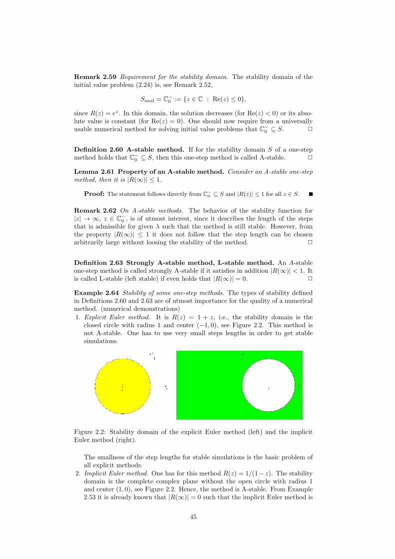
1. Explicit Euler method. It is R(z) = 1 + z, i.e., the stability domain is theclosed circle with radius 1 and center (−1, 0), see Figure 2.2. This method isnot A-stable. One has to use very small steps lengths in order to get stablesimulations.

Figure 2.2: Stability domain of the explicit Euler method (left) and the implicitEuler method (right).

The smallness of the step lengths for stable simulations is the basic problem ofall explicit methods.

2. Implicit Euler method. One has for this method R(z) = 1/(1− z). The stabilitydomain is the complete complex plane without the open circle with radius 1and center (1, 0), see Figure 2.2. Hence, the method is A-stable. From Example2.53 it is already known that |R(∞)| = 0 such that the implicit Euler method is

45

even L-stable. A smallness condition on the step lengths does not arise for thismethod, at least for the model problem (2.24).In general, one can apply in the implicit Euler method much larger steps than,e.g., in the explicit Euler method. Step size restrictions arise, e.g., from thephysics of the problem and from the required accuracy of the simulations. How-ever, one has to solve in general in each node a nonlinear equation, like for eachimplicit scheme. Thus, the numerical costs and the computing time per step areusually much larger than for explicit schemes.

3. Trapezoidal rule. For the trapezoidal rule, one gets with z = a+ ib

|R(z)|2 =

∣∣∣∣

1 + z/2

1− z/2

∣∣∣∣

2

=

∣∣∣∣

1 + a/2 + ib/2

1− a/2− ib/2

∣∣∣∣

2

=(2 + a)2 + b2

(2− a)2 + b2.

It follows that

R(z) =

< 1 for a < 0 ⇐⇒ Re(z) < 0,= 1 for a = 0 ⇐⇒ Re(z) = 0,= 1 z = ∞.

Hence, one obtains S = C−0 . This method is A-stable but not L-stable. However,

in contrast to the implicit Euler method, which is a first order method, thetrapezoidal rule is a second order method.

2

Remark 2.65 Extension of the theory to linear systems. Consider the linear sys-tem of ordinary differential equations with constant coefficients

y′(x) = Ay(x), y(0) = y0, A ∈ Rn×n, y0 ∈ R

n. (2.25)

It will be assumed that the matrix A possesses n mutually different eigenvaluesλ1, . . . , λn ∈ C. The solution of (2.25) has the form, see (2.21),

y(x) = eAxy0.

Since A has n mutually different eigenvalues, this matrix can be diagonalized,i.e., there exists a matrix Q ∈ R

n×n such that

Λ = Q−1AQ, with Λ = diag(λ1, . . . , λn).

The columns qi of Q are the eigenvectors of A. Using the substitution

y(x) = Qz(x) =⇒ y′(x) = Qz′(x),

one obtains the differential equation

Qz′(x) = AQz(x) ⇐⇒ z′(x) = Q−1AQz(x) = Λz(x).

The equations of this system are decoupled. Its general solution is given by

z(x) = eΛxc =(cie

λix)

i=1,...,n.

It follows that the general solution of (2.25) has the form

y(x) = Qz(x) =

n∑

i=1

cieλixqi.

Inserting this expression into the initial value problem gives

y(0) =

n∑

i=1

ciqi = Qc = y0 =⇒ c = Q−1y0.

46

Hence, one obtains the following solution of the initial value problem

y(x) =n∑

i=1

(Q−1y0

)

ieλixqi, (2.26)

where ((Q−1y0

)

iis the i-th component of Q−1y0. Now, one can easily see that

the solution is stable (small changes of the initial data lead to small changes of thesolution) only if all eigenvalues have a negative real part.

The consideration of numerical methods makes sense only in the case that theproblem is well posed, i.e., all eigenvalues have a negative real part. Then, the mostimportant term in (2.26) with respect to stability is the term with the eigenvalueof A with the largest absolute value of its real part. 2

Definition 2.66 Stiff system of ordinary differential equations. The linearsystem of ordinary differential equations

y′(x) = Ay(x), A ∈ Rn×n,

is called stiff, if all eigenvalues λi of A possess a negative real part and if

q :=max{Re(λi), i = 1, . . . , n}min{Re(λi), i = 1, . . . , n} � 1.

Sometimes, the system is called weakly stiff if q ≈ 10 and stiff if q > 10. 2

Remark 2.67 On Definition 2.66. Definition 2.66 has a disadvantage. The ratiobecomes large also in the case that the eigenvalue with the smallest absolute valueof the real part is close to zero. However, this eigenvalue is not important for thestability, only the eigenvalue with the largest absolute value of the real part. 2

Remark 2.68 Local stiffness for general ordinary differential equations. The no-tation of stiffness can be extended in some sense from linear differential equationsto general differential equations. The differential equation

y′(x) = f(x,y(x))

can be transformed, by introducing the functions

y(x) := x and y(x) :=

(y(x)y(x)

)

,

to the autonomous form

y′(x) = f (y(x)) =

(f(x,y(x))

1

)

.

By linearizing at the initial value y0, one obtains a differential equation of the formy′(x) = Ay(x). Applying some definition of stiffness to the linearized equation, itis possible to define a local stiffness for the general equation.

However, if one considers nonlinear problems, one has to be careful in the inter-pretation of the results. In general, the results are valid only locally and they donot describe the behavior of a numerical method in the whole domain of definitionof the nonlinear problem. 2

47

2.6 Rosenbrock Methods

Remark 2.69 Goal. From the stability theory it became obvious that one hasto use implicit methods for stiff problems. However, implicit methods are compu-tationally expensive, one has to solve in general nonlinear problems in each step.The goal consists in defining implicit methods that have on the one hand a reducedcomputational complexity but on the other hand, they should be still accurate andstable. 2

Remark 2.70 Linearly implicit Runge–Kutta method. Consider, without loss ofgenerality, the autonomous initial value problem

y′(x) = f(y), y(0) = y0,

see Remark 1.30. DIRK methods, see Remark 2.51, has a Butcher tableau of theform

c1 a11 0 0 · · · 0c2 a21 a22 0 · · · 0c3 a31 a32 a33 · · · 0...

......

. . .

cs as1 as2 · · · assb1 b2 · · · bs−1 bs

.

One has to solve s decoupled nonlinear equations

Kj = f

(

yk + h

j−1∑

l=1

ajlKl + hajjKj

)

, j = 1, . . . , s.

The quasi Newton method for solving the j-th equation leads to an iterative schemeof the form

K(n+1)j = K

(n)j − (I − ajjhJ)

−1

[

K(n)j − f

(

yk + h

j−1∑

l=1

ajlKl + hajjK(n)j

)]

,

n = 0, 1, . . .. In this scheme, one uses usually the approximation of the derivativeJ = fy(yk) instead of the derivative at the current iterate, hence it is a quasi Newtonmethod. If the step length h is sufficiently small, then the matrix (I − ajjhJ) isnon-singular and the linear systems of equations possess a unique solution.

Often, it turns out to be sufficient for reaching the required accuracy to performjust one step of the iteration. This statement holds in particular if the step length

is sufficiently small and if a sufficiently accurate start value K(0)j is available. With

the ansatz (linear combination of the already computed stages)

K(0)j :=

j−1∑

l=1

djlajj

Kl,

where the coefficients djl, l = 1, . . . , j − 1, still need to be determined, one obtainsan implicit method with linear systems of equations

(I − ajjhJ)Kj = f

(

yk + h

j−1∑

l=1

(ajl + djl)Kl

)

− hJ

j−1∑

l=1

djlKl, j = 1, . . . , s,

yk+1 = yk + hs∑

j=1

bjKj . (2.27)

48

This class of methods is called linearly implicit Runge–Kutta methods.Linearly implicit Runge–Kutta methods are still implicit methods. One has to

solve in each step only s linear systems of equations. That means, these methodsare considerably less computational complex than the original implicit methodsand the first goal stated in Remark 2.69 is achieved. Now, one has to study whichproperties of the original methods are transferred to the linearly implicit methods.In particular, stability is of importance. If stability will be lost, then the linearlyimplicit methods are not suited for solving stiff differential equations. 2

Theorem 2.71 Stability of linearly implicit Runge–Kutta methods. Con-sider a Runge–Kutta method with the parameters (A,b, c), where A ∈ R

s×s isa non-singular lower triangular matrix. Then, the corresponding linearly implicitRunge–Kutta method (2.27) with J = fy(yk) has the same stability function R(z)as the original method, independently of the choice of {djl}.

Proof: The linearly implicit method will be applied to the one-dimensional (to sim-plify notations) test problem

y′(x) = λy(x), y(0) = 1,

with Re(λ) < 0. Since f(y) = λy, one obtains J = λ. The j-th equation of (2.27) has theform

(I − ajjhλ)Kj = λ

(

yk + h

j−1∑

l=1

(ajl + djl)Kl

)

− hλ

j−1∑

l=1

djlKl

= λyk + hλ

j−1∑

l=1

ajlKl, j = 1, . . . , s.

Multiplication with h gives with z = λh

Kjh− z

j∑

l=1

ajlKlh = zyk, j = 1, . . . , s.

This equation is equivalent, using matrix-vector notations, to

(I − zA)Kh = zyk1, K = (K1, . . . ,Ks)T .

Let h be chosen in such a way that z is not an eigenvalue of A. Then, one obtains byinserting this equation into the second equation of (2.27)

yk+1 = yk + hbTK = yk + hbT (I − zA)−1

1z

hyk =

(

1 + zbT (I − zA)−11)

yk = R(z)yk.

Now one can see that in the parentheses there is the stability function R(z) of the original

Runge–Kutta method, see Definition 2.54.

Remark 2.72 On the stability and consistency. Since the most important stabilityproperties of a numerical method for solving ordinary differential equations dependonly on the stability function, these properties transfer from the original implicitRunge–Kutta method to the corresponding linearly implicit method.

The choice of the coefficients {djl} will influence the order of the linearly implicitmethod. For an inappropriate choice of these coefficients, the order of the linearlyimplicit method might be lower than the order of the original method. 2

Example 2.73 Linearly implicit Euler method. The implicit Euler method has theButcher tableau

1 11

49

With (2.27), it follows that the linearly implicit Euler method has the form

(I − hfy(yk))K1 = f (yk) , yk+1 = yk + hK1

The linearly implicit Euler method is L-stable, like the implicit Euler method, andone has to solve in each step only one linear system of equations. There are nocoefficients djl to be chosen in this method. 2

Remark 2.74 Rosenbrock7 methods. Another possibility for simplifying the usageof linearly implicit methods and decreasing the numerical costs consists in usingfor all stages the same coefficient ajj = a. In this case, all linear systems of equa-tions in (2.27) possess the same system matrix (I − ahJ). Then, one nees only oneLU decomposition of this matrix and can solve all systems in (2.27) with this de-composition. This approach is called Rosenbrock methods or Rosenbrock–Wanner8

methods (ROW methods)

(I − ahJ)Kj = f

(

yk + h

j−1∑

l=1

(ajl + djl)Kl

)

− hJ

j−1∑

l=1

djlKl, j = 1, . . . , s,(2.28)

yk+1 = yk + h

s∑

j=1

bjKj .

In practice, it is often even possible to use the same approximation J of theJacobian for some subsequent steps. This is true in particular, if the solutionchanges only slowly. In this way, one can save additional computational costs. 2

Example 2.75 The method ode23s. In MATLAB, one can find for solving stiffordinary differential equations the Rosenbrock method ode23s, see Shampine andReichelt (1997). This method has the form

(I − ahJ)K1 = f(yk), a =1

2 +√2≈ 0.2928932,

(I − ahJ)K2 = f

(

yk +1

2hK1

)

− ahJK1,

yk+1 = yk + hK2.

From the equation for the second stage, it follows that d21 = a. Then, one obtainswith (2.28) a21 = 1/2− d21 = 1/2− a. Using the condition that the nodes are thesums of the rows of the matrix, it follows that the corresponding Butcher tableaulooks like

a a1/2 1/2− a a

0 1.

2

Theorem 2.76 Order of ode23s. The Rosenbrock method ode23s is of secondorder.

Proof: Let h ∈ (0, 1/(2a ‖J‖2)), where ‖·‖2 denotes the spectral norm of J , whichis induced by the Euclidean vector norm ‖·‖2. It can be shown, see class ComputerMathematics, that the matrix (I − ahJ) is invertible if ‖ahJ‖2 < 1. This condition issatisfied for the choice of h from above.

7Howard H. Rosenbrock (1920 – 2010)8Gerhard Wanner, born 1942

50

Let K be the solution of(I − ahJ)K = f .

Then, one obtains with the triangle inequality, with the compatibility of the Euclideanvector norm and the spectral matrix norm, and with the choice of h that

‖(I − ahJ)K‖2 ≥ ‖K‖2 − ah ‖JK‖2 ≥ ‖K‖2 − ah ‖J‖2 ‖K‖2

≥ ‖K‖2 −a ‖J‖22a ‖J‖2

‖K‖2 =1

2‖K‖2 .

It follows, using the linear system of equations, that

1

2‖K‖2 ≤ ‖(I − ahJ)K‖2 = ‖f‖2 ⇐⇒ ‖K‖2 ≤ 2 ‖f‖2 .

Thus, the solution of the linear system of equations is bounded by the right hand side.One obtains for the first stage of ode23s by recursive insertion

K1 = f(yk) + ahJK1 = f(yk) + ahJ (f(yk) + ahJK1)

= f(yk) + ahJf(yk) + h2a2J2K1

= f(yk) + ahJf(yk) +O(h2) . (2.29)

The last step is allowed since K1 is bounded by the data of the problem (the right handside f(yk)) independently of h. Using a Taylor series expansion and considering only firstorder terms explicitly, one obtains in a similar way for the second stage of ode23s

K2 = f

(

yk +1

2hK1

)

− ahJK1 + ahJK2

= f (yk) +1

2hfy (yk)K1 − ahJK1 + ahJK2 +O

(h2)

(2.29)= f (yk) +

1

2hfy (yk) f (yk)− ahJf(yk) + ahJK2 +O

(h2)

= f (yk) +1

2hfy (yk) f (yk)− ahJf(yk) + ahJf(yk) +O

(h2)

= f (yk) +1

2hfy (yk) f (yk) +O

(h2) .

Inserting these results gives for on step of ode23s

yk+1 = yk + hf (yk) +1

2h2

fy (yk) f (yk) +O(h3) . (2.30)

The Taylor series expansion of the solution y(x) of the system of differential equations inxk has the form, using the differential equation,

y(xk+1) = y(xk) + hy′(xk) +h2

2y′′(xk) +O

(h3)

= y(xk) + hf (yk) +h2

2

∂f (y)

∂x(xk) +O

(h3)

= y(xk) + hf (yk) +h2

2fy (yk)y

′(xk) +O(h3)

= y(xk) + hf (yk) +h2

2fy (yk) f (yk) +O

(h3) .

Starting with the exact value, then the first three terms of (2.30) correspond to the Taylor

series expansion of the solution y(x) of the system of differential equations in xk. Thus,

it follows that the local error is of order O(h3), from what follows that the consistency

order of ode23s is two, see Definition 1.14.

Remark 2.77 To the proof of Theorem 2.76. Note that it is not needed in theproof of Theorem 2.76 that J is the exact derivative fy (yk). The method ode23s

remains a second order method if J is only an approximation of fy (yk) and evenif J is an arbitrary matrix. However, the transfer of the stability properties fromthe original method to ode23s is only guarantied for the choice J = fy (yk), seeTheorem 2.71. 2

51

Theorem 2.78 Stability function of ode23s. Assume that J = fy(yk), then thestability function of the Rosenbrock method ode23s has the form

R(z) =1 + (1− 2a)z

(1− az)2.

Proof: The statement of the theorem follows from applying the method to the usual

test equation, exercise.

Remark 2.79 On the order of ode23s. It remains the question if an appropriatechoice of J might even increase the order of the method. However, for the modelproblem of the stability analysis, a series expansion of the stability function showsthat the exponential function is reproduced exactly only to the third term. Fromthis observation it follows that one does not obtain a third order method even withexact Jacobian. In practice, there is no important reason from the point of view ofaccuracy to compute a new Jacobian in each step. Often, it is sufficient to updatethe J every now and then. 2

Cororllary 2.80 Stability of ode23s. If J = fy(yk), then the Rosenbrock methodode23s is L-stable.

Proof: The statement is obtained by applying the definition of L-stability to the

stability function.

52