Cartan for Beginners:

Differential Geometry via Moving Frames

and Exterior Differential Systems

Thomas A. Ivey and J.M. Landsberg

Contents

Preface ix

Chapter 1. Moving Frames and Exterior Differential Systems 1

§1.1. Geometry of surfaces in E3 in coordinates 2

§1.2. Differential equations in coordinates 5

§1.3. Introduction to differential equations without coordinates 8

§1.4. Introduction to geometry without coordinates:curves in E2 12

§1.5. Submanifolds of homogeneous spaces 15

§1.6. The Maurer-Cartan form 16

§1.7. Plane curves in other geometries 20

§1.8. Curves in E3 23

§1.9. Exterior differential systems and jet spaces 26

Chapter 2. Euclidean Geometry and Riemannian Geometry 35

§2.1. Gauss and mean curvature via frames 36

§2.2. Calculation of H and K for some examples 39

§2.3. Darboux frames and applications 42

§2.4. What do H and K tell us? 43

§2.5. Invariants for n-dimensional submanifolds of En+s 45

§2.6. Intrinsic and extrinsic geometry 47

§2.7. Space forms: the sphere and hyperbolic space 57

§2.8. Curves on surfaces 58

§2.9. The Gauss-Bonnet and Poincare-Hopf theorems 61

v

vi Contents

§2.10. Non-orthonormal frames 66

Chapter 3. Projective Geometry 71

§3.1. Grassmannians 72

§3.2. Frames and the projective second fundamental form 76

§3.3. Algebraic varieties 81

§3.4. Varieties with degenerate Gauss mappings 89

§3.5. Higher-order differential invariants 94

§3.6. Fundamental forms of some homogeneous varieties 98

§3.7. Higher-order Fubini forms 107

§3.8. Ruled and uniruled varieties 113

§3.9. Varieties with vanishing Fubini cubic 115

§3.10. Dual varieties 118

§3.11. Associated varieties 123

§3.12. More on varieties with degenerate Gauss maps 125

§3.13. Secant and tangential varieties 128

§3.14. Rank restriction theorems 132

§3.15. Local study of smooth varieties with degenerate tangentialvarieties 134

§3.16. Generalized Monge systems 137

§3.17. Complete intersections 139

Chapter 4. Cartan-Kahler I: Linear Algebra and Constant-CoefficientHomogeneous Systems 143

§4.1. Tableaux 144

§4.2. First example 148

§4.3. Second example 150

§4.4. Third example 153

§4.5. The general case 154

§4.6. The characteristic variety of a tableau 157

Chapter 5. Cartan-Kahler II: The Cartan Algorithm for LinearPfaffian Systems 163

§5.1. Linear Pfaffian systems 163

§5.2. First example 165

§5.3. Second example: constant coefficient homogeneous systems 166

§5.4. The local isometric embedding problem 169

Contents vii

§5.5. The Cartan algorithm formalized:tableau, torsion and prolongation 173

§5.6. Summary of Cartan’s algorithm for linear Pfaffian systems 177

§5.7. Additional remarks on the theory 179

§5.8. Examples 182

§5.9. Functions whose Hessians commute, with remarks on singularsolutions 189

§5.10. The Cartan-Janet Isometric Embedding Theorem 191

§5.11. Isometric embeddings of space forms (mostly flat ones) 194

§5.12. Calibrated submanifolds 197

Chapter 6. Applications to PDE 203

§6.1. Symmetries and Cauchy characteristics 204

§6.2. Second-order PDE and Monge characteristics 212

§6.3. Derived systems and the method of Darboux 215

§6.4. Monge-Ampere systems and Weingarten surfaces 222

§6.5. Integrable extensions and Backlund transformations 231

Chapter 7. Cartan-Kahler III: The General Case 243

§7.1. Integral elements and polar spaces 244

§7.2. Example: Triply orthogonal systems 251

§7.3. Statement and proof of Cartan-Kahler 254

§7.4. Cartan’s Test 256

§7.5. More examples of Cartan’s Test 259

Chapter 8. Geometric Structures and Connections 267

§8.1. G-structures 267

§8.2. How to differentiate sections of vector bundles 275

§8.3. Connections on FG and differential invariants of G-structures 278

§8.4. Induced vector bundles and connections on induced bundles 283

§8.5. Holonomy 286

§8.6. Extended example: Path geometry 295

§8.7. Frobenius and generalized conformal structures 308

Appendix A. Linear Algebra and Representation Theory 311

§A.1. Dual spaces and tensor products 311

§A.2. Matrix Lie groups 316

§A.3. Complex vector spaces and complex structures 318

viii Contents

§A.4. Lie algebras 320

§A.5. Division algebras and the simple group G2 323

§A.6. A smidgen of representation theory 326

§A.7. Clifford algebras and spin groups 330

Appendix B. Differential Forms 335

§B.1. Differential forms and vector fields 335

§B.2. Three definitions of the exterior derivative 337

§B.3. Basic and semi-basic forms 339

§B.4. Differential ideals 340

Appendix C. Complex Structures and Complex Manifolds 343

§C.1. Complex manifolds 343

§C.2. The Cauchy-Riemann equations 347

Appendix D. Initial Value Problems 349

Hints and Answers to Selected Exercises 355

Bibliography 363

Index 371

Preface

In this book, we use moving frames and exterior differential systems to studygeometry and partial differential equations. These ideas originated abouta century ago in the works of several mathematicians, including GastonDarboux, Edouard Goursat and, most importantly, Elie Cartan. Over theyears these techniques have been refined and extended; major contributorsto the subject are mentioned below, under “Further Reading”.

The book has the following features: It concisely covers the classicalgeometry of surfaces and basic Riemannian geometry in the language ofmoving frames. It includes results from projective differential geometry thatupdate and expand the classic paper [69] of Griffiths and Harris. It providesan elementary introduction to the machinery of exterior differential systems(EDS), and an introduction to the basics of G-structures and the generaltheory of connections. Classical and recent geometric applications of thesetechniques are discussed throughout the text.

This book is intended to be used as a textbook for a graduate-levelcourse; there are numerous exercises throughout. It is suitable for a one-year course, although it has more material than can be covered in a year, andparts of it are suitable for one-semester course (see the end of this preface forsome suggestions). The intended audience is both graduate students whohave some familiarity with classical differential geometry and differentiablemanifolds, and experts in areas such as PDE and algebraic geometry whowant to learn how moving frame and EDS techniques apply to their fields.

In addition to the geometric applications presented here, EDS techniquesare also applied in CR geometry (see, e.g., [98]), robotics, and control theory(see [55, 56, 129]). This book prepares the reader for such areas, as well as

ix

x Preface

for more advanced texts on exterior differential systems, such as [20], andpapers on recent advances in the theory, such as [58, 117].

Overview. Each section begins with geometric examples and problems.Techniques and definitions are introduced when they become useful to helpsolve the geometric questions under discussion. We generally keep the pre-sentation elementary, although advanced topics are interspersed throughoutthe text.

In Chapter 1, we introduce moving frames via the geometry of curves inthe Euclidean plane E2. We define the Maurer-Cartan form of a Lie group Gand explain its use in the study of submanifolds of G-homogeneous spaces.We give additional examples, including the equivalence of holomorphic map-pings up to fractional linear transformation, where the machinery leads onenaturally to the Schwarzian derivative.

We define exterior differential systems and jet spaces, and explain howto rephrase any system of partial differential equations as an EDS using jets.We state and prove the Frobenius system, leading up to it via an elementaryexample of an overdetermined system of PDE.

In Chapter 2, we cover traditional material—the geometry of surfaces inthree-dimensional Euclidean space, submanifolds of higher-dimensional Eu-clidean space, and the rudiments of Riemannian geometry—all using movingframes. Our emphasis is on local geometry, although we include standardglobal theorems such as the rigidity of the sphere and the Gauss-BonnetTheorem. Our presentation emphasizes finding and interpreting differentialinvariants to enable the reader to use the same techniques in other settings.

We begin Chapter 3 with a discussion of Grassmannians and the Pluckerembedding. We present some well-known material (e.g., Fubini’s theorem onthe rigidity of the quadric) which is not readily available in other textbooks.We present several recent results, including the Zak and Landman theoremson the dual defect, and results of the second author on complete intersec-tions, osculating hypersurfaces, uniruled varieties and varieties covered bylines. We keep the use of terminology and results from algebraic geometryto a minimum, but we believe we have included enough so that algebraicgeometers will find this chapter useful.

Chapter 4 begins our multi-chapter discussion of the Cartan algorithmand Cartan-Kahler Theorem. In this chapter we study constant coefficienthomogeneous systems of PDE and the linear algebra associated to the corre-sponding exterior differential systems. We define tableaux and involutivityof tableaux. One way to understand the Cartan-Kahler Theorem is as fol-lows: given a system of PDE, if the linear algebra at the infinitesimal level

Preface xi

“works out right” (in a way explained precisely in the chapter), then exis-tence of solutions follows.

In Chapter 5 we present the Cartan algorithm for linear Pfaffian systems,a very large class of exterior differential systems that includes systems ofPDE rephrased as exterior differential systems. We give numerous examples,including many from Cartan’s classic treatise [31], as well as the isometricimmersion problem, problems related to calibrated submanifolds, and anexample motivated by variation of Hodge structure.

In Chapter 6 we take a detour to discuss the classical theory of character-istics, Darboux’s method for solving PDE, and Monge-Ampere equations inmodern language. By studying the exterior differential systems associatedto such equations, we recover the sine-Gordon representation of pseudo-spherical surfaces, the Weierstrass representation of minimal surfaces, andthe one-parameter family of non-congruent isometric deformations of a sur-face of constant mean curvature. We also discuss integrable extensions andBacklund transformations of exterior differential systems, and the relation-ship between such transformations and Darboux integrability.

In Chapter 7, we present the general version of the Cartan-Kahler The-orem. Doing so involves a detailed study of the integral elements of an EDS.In particular, we arrive at the notion of a Kahler-regular flag of integral ele-ments, which may be understood as the analogue of a sequence of well-posedCauchy problems. After proving both the Cartan-Kahler Theorem and Car-tan’s test for regularity, we apply them to several examples of non-Pfaffiansystems arising in submanifold geometry.

Finally, in Chapter 8 we give an introduction to geometric structures(G-structures) and connections. We arrive at these notions at a leisurelypace, in order to develop the intuition as to why one needs them. Ratherthan attempt to describe the theory in complete generality, we present oneextended example, path geometry in the plane, to give the reader an ideaof the general theory. We conclude with a discussion of some recent gener-alizations of G-structures and their applications.

There are four appendices, covering background material for the mainpart of the book: linear algebra and rudiments of representation theory,differential forms and vector fields, complex and almost complex manifolds,and a brief discussion of initial value problems and the Cauchy-KowalevskiTheorem, of which the Cartan-Kahler Theorem is a generalization.

xii Preface

Layout. All theorems, propositions, remarks, examples, etc., are numberedtogether within each section; for example, Theorem 1.3.2 is the second num-bered item in section 1.3. Equations are numbered sequentially within eachchapter. We have included hints for selected exercises, those marked withthe symbol at the end, which is meant to be suggestive of a life preserver.

Further Reading on EDS. To our knowledge, there are only a smallnumber of textbooks on exterior differential systems. The first is Cartan’sclassic text [31], which has an extraordinarily beautiful collection of ex-amples, some of which are reproduced here. We learned the subject fromour teacher Bryant and the book by Bryant, Chern, Griffiths, Gardner andGoldschmidt [20], which is an elaboration of an earlier monograph [19], andis at a more advanced level than this book. One text at a comparable levelto this book, but more formal in approach, is [156]. The monograph [70],which is centered around the isometric embedding problem, is similar inspirit but covers less material. The memoir [155] is dedicated to extendingthe Cartan-Kahler Theorem to the C∞ setting for hyperbolic systems, butcontains an exposition of the general theory. There is also a monographby Kahler [89] and lectures by Kuranishi [97], as well the survey articles[66, 90]. Some discussion of the theory may be found in the differentialgeometry texts [142] and [145].

We give references for other topics discussed in the book in the text.

History and Acknowledgements. This book started out about a decadeago. We thought we would write up notes from Robert Bryant’s Tuesdaynight seminar, held in 1988–89 while we were graduate students, as wellas some notes on exterior differential systems which would be more intro-ductory than [20]. The seminar material is contained in §8.6 and parts ofChapter 6. Chapter 2 is influenced by the many standard texts on the sub-ject, especially [43] and [142], while Chapter 3 is influenced by the paper[69]. Several examples in Chapter 5 and Chapter 7 are from [31], and theexamples of Darboux’s method in Chapter 6 are from [63]. In each case,specific attributions are given in the text. Chapter 7 follows Chapter III of[20] with some variations. In particular, to our knowledge, Lemmas 7.1.10and 7.1.13 are original. The presentation in §8.5 is influenced by [11], [94]and unpublished lectures of Bryant.

The first author has given graduate courses based on the material inChapters 6 and 7 at the University of California, San Diego and at CaseWestern Reserve University. The second author has given year-long gradu-ate courses using Chapters 1, 2, 4, 5, and 8 at the University of Pennsylvaniaand Universite de Toulouse III, and a one-semester course based on Chap-ters 1, 2, 4 and 5 at Columbia University. He has also taught one-semester

Preface xiii

undergraduate courses using Chapters 1 and 2 and the discussion of con-nections in Chapter 8 (supplemented by [141] and [142] for backgroundmaterial) at Toulouse and at Georgia Institute of Technology, as well asone-semester graduate courses on projective geometry from Chapters 1 and3 (supplemented by some material from algebraic geometry), at Toulouse,Georgia Tech. and the University of Trieste. He also gave more advancedlectures based on Chapter 3 at Seoul National University, which were pub-lished as [107] and became a precursor to Chapter 3. Preliminary versionsof Chapters 5 and 8 respectively appeared in [104, 103].

We would like to thank the students in the above classes for their feed-back. We also thank Megan Dillon, Phillipe Eyssidieux, Daniel Fox, Sung-Eun Koh, Emilia Mezzetti, Joseph Montgomery, Giorgio Ottaviani, JensPiontkowski, Margaret Symington, Magdalena Toda, Sung-Ho Wang andPeter Vassiliou for comments on the earlier drafts of this book, and An-nette Rohrs for help with the figures. The staff of the publications divisionof the AMS—in particular, Ralph Sizer, Tom Kacvinsky, and our editor,Ed Dunne—were of tremendous help in pulling the book together. We aregrateful to our teacher Robert Bryant for introducing us to the subject.Lastly, this project would not have been possible without the support andpatience of our families.

xiv Preface

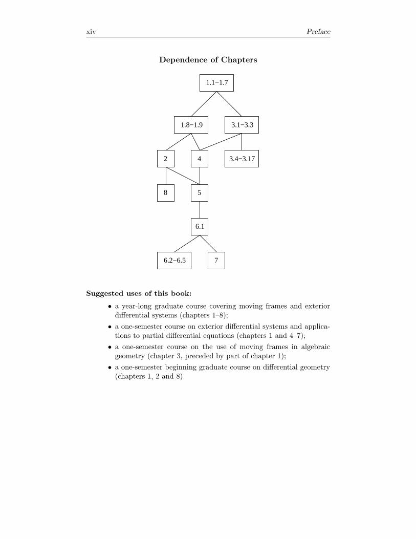
Dependence of Chapters

3.1−3.3

3.4−3.174

58

1.1−1.7

6.1

7

2

1.8−1.9

6.2−6.5

Suggested uses of this book:

• a year-long graduate course covering moving frames and exteriordifferential systems (chapters 1–8);

• a one-semester course on exterior differential systems and applica-tions to partial differential equations (chapters 1 and 4–7);

• a one-semester course on the use of moving frames in algebraicgeometry (chapter 3, preceded by part of chapter 1);

• a one-semester beginning graduate course on differential geometry(chapters 1, 2 and 8).

Chapter 1

Moving Frames andExterior DifferentialSystems

In this chapter we motivate the use of differential forms to study problemsin geometry and partial differential equations. We begin with familiar ma-terial: the Gauss and mean curvature of surfaces in E3 in §1.1, and Picard’sTheorem for local existence of solutions of ordinary differential equations in§1.2. We continue in §1.2 with a discussion of a simple system of partial dif-ferential equations, and then in §1.3 rephrase it in terms of differential forms,which facilitates interpreting it geometrically. We also state the FrobeniusTheorem.

In §1.4, we review curves in E2 in the language of moving frames. Wegeneralize this example in §§1.5–1.6, describing how one studies subman-ifolds of homogeneous spaces using moving frames, and introducing theMaurer-Cartan form. We give two examples of the geometry of curves in ho-mogeneous spaces: classifying holomorphic mappings of the complex planeunder fractional linear transformations in §1.7, and classifying curves in E3

under Euclidean motions (i.e., rotations and translations) in §1.8. We alsoinclude exercises on plane curves in other geometries.

In §1.9, we define exterior differential systems and integral manifolds.We prove the Frobenius Theorem, give a few basic examples of exterior dif-ferential systems, and explain how to express a system of partial differentialequations as an exterior differential system using jet bundles.

1

2 1. Moving Frames and Exterior Differential Systems

Throughout this book we use the summation convention: unless other-wise indicated, summation is implied whenever repeated indices occur upand down in an expression.

1.1. Geometry of surfaces in E3 in coordinates

Let E3 denote Euclidean three-space, i.e., the affine space R3 equipped withits standard inner product.

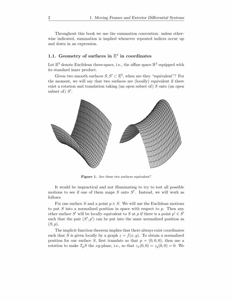
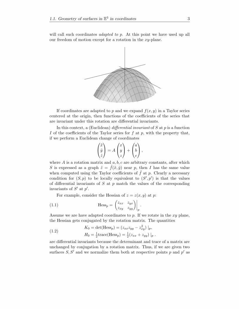
Given two smooth surfaces S, S ′ ⊂ E3, when are they “equivalent”? Forthe moment, we will say that two surfaces are (locally) equivalent if thereexist a rotation and translation taking (an open subset of) S onto (an opensubset of) S ′.

Figure 1. Are these two surfaces equivalent?

It would be impractical and not illuminating to try to test all possiblemotions to see if one of them maps S onto S ′. Instead, we will work asfollows:

Fix one surface S and a point p ∈ S. We will use the Euclidean motionsto put S into a normalized position in space with respect to p. Then anyother surface S ′ will be locally equivalent to S at p if there is a point p′ ∈ S′such that the pair (S ′, p′) can be put into the same normalized position as(S, p).

The implicit function theorem implies that there always exist coordinatessuch that S is given locally by a graph z = f(x, y). To obtain a normalizedposition for our surface S, first translate so that p = (0, 0, 0), then use arotation to make TpS the xy-plane, i.e., so that zx(0, 0) = zy(0, 0) = 0. We

1.1. Geometry of surfaces in E3 in coordinates 3

will call such coordinates adapted to p. At this point we have used up allour freedom of motion except for a rotation in the xy-plane.

If coordinates are adapted to p and we expand f(x, y) in a Taylor seriescentered at the origin, then functions of the coefficients of the series thatare invariant under this rotation are differential invariants.

In this context, a (Euclidean) differential invariant of S at p is a functionI of the coefficients of the Taylor series for f at p, with the property that,if we perform a Euclidean change of coordinates

xyz

= A

xyz

+

abc

,

where A is a rotation matrix and a, b, c are arbitrary constants, after whichS is expressed as a graph z = f(x, y) near p, then I has the same value

when computed using the Taylor coefficients of f at p. Clearly a necessarycondition for (S, p) to be locally equivalent to (S ′, p′) is that the valuesof differential invariants of S at p match the values of the correspondinginvariants of S ′ at p′.

For example, consider the Hessian of z = z(x, y) at p:

Hessp =

(zxx zyxzxy zyy

)∣∣∣∣p

.(1.1)

Assume we are have adapted coordinates to p. If we rotate in the xy plane,the Hessian gets conjugated by the rotation matrix. The quantities

K0 = det(Hessp) = (zxxzyy − z2xy) |p,H0 =

12trace(Hessp) =

12(zxx + zyy) |p .

(1.2)

are differential invariants because the determinant and trace of a matrix areunchanged by conjugation by a rotation matrix. Thus, if we are given twosurfaces S, S ′ and we normalize them both at respective points p and p′ as

4 1. Moving Frames and Exterior Differential Systems

above, a necessary condition for there to be a rigid motion taking p′ to psuch that the Taylor expansions for the two surfaces at the point p coincideis that K0(S) = K0(S

′) and H0(S) = H0(S′).

The formulas (1.2) are only valid at one point, and only after the surfacehas been put in normalized position relative to that point. To calculate Kand H as functions on S it would be too much work to move each point tothe origin and arrange its tangent plane to be horizontal. But it is possi-ble to adjust the formulas to account for tilted tangent planes (see §2.10).One then obtains the following functions, which are differential invariantsunder Euclidean motions of surfaces that are locally described as graphsz = z(x, y):

K(x, y) =zxxzyy − z2xy(1 + z2x + z2y)

2,

H(x, y) =1

2

(1 + z2y)zxx − 2zxzyzxy + (1 + z2x)zyy

(1 + z2x + z2y)32

,

(1.3)

respectively giving the Gauss and mean curvature of S at p = (x, y, z(x, y)).

Exercise 1.1.1: By locally describing each surface as a graph, calculate theGauss and mean curvature functions for a sphere of radius R, a cylinder ofradius r (e.g., x2+ y2 = r2) and the smooth points of the cone x2+ y2 = z2.

Once one has found invariants for a given submanifold geometry, onemay ask questions about submanifolds with special invariants. For surfacesin E3, one might ask which surfaces have K constant or H constant. Thesecan be treated as questions about solutions to certain partial differentialequations (PDE). For example, from (1.3) we see that surfaces with K ≡ 1are locally given by solutions to the PDE

zxxzyy − z2xy = (1 + z2x + z2y)2.(1.4)

We will soon free ourselves of coordinates and use moving frames and dif-ferential forms. As a provisional definition, a moving frame is a smoothlyvarying basis of the tangent space to E3 defined at each point of our sur-face. In general, using moving frames one can obtain formulas valid at everypoint analogous to coordinate formulas valid at just one preferred point. Inthe present context, the Gauss and mean curvatures will be described at allpoints by expressions like (1.2) rather than (1.3); see §2.1.

Another reason to use moving frames is that the method gives a uni-form procedure for dealing with diverse geometric settings. Even if one isoriginally only interested in Euclidean geometry, other geometries arise nat-urally. For example, consider the warp of a surface, which is defined to be(k1 − k2)2, where the kj are the eigenvalues of (1.1). It turns out that this

1.2. Differential equations in coordinates 5

quantity is invariant under a larger change of coordinates than the Eucli-dean group, namely conformal changes of coordinates, and thus it is easierto study the warp in the context of conformal geometry.

Regardless of how unfamiliar a geometry initially appears, the method ofmoving frames provides an algorithm to find differential invariants. Thus wewill have a single method for dealing with conformal, Hermitian, projectiveand other geometries. Because it is familiar, we will often use the geometryof surfaces in E3 as an example, but the reader should keep in mind thatthe beauty of the method is its wide range of applicability. As for the useof differential forms, we shall see that when we express a system of PDE asan exterior differential system, the geometric features of the system—i.e.,those which are independent of coordinates—will become transparent.

1.2. Differential equations in coordinates

The first questions one might ask when confronted with a system of differ-ential equations are: Are there any solutions? If so, how many?

In the case of a single ordinary differential equation (ODE), here is theanswer:

Theorem 1.2.1 (Picard1). Let f(x, u) : R2 → R be a function with f andfu continuous. Then for all (x0, u0) ∈ R2, there exist an open interval I 3 x0and a function u(x) defined on I, satisfying u(x0) = u0 and the differentialequation

du

dx= f(x, u).(1.5)

Moreover, any other solution of this initial value problem must coincide withthis solution on I.

In other words, for a given ODE there exists a solution defined near x0and this solution is unique given the choice of a constant u0. Thus for anODE for one function of one variable, we say that solutions depend on oneconstant. More generally, Picard’s Theorem applies to systems of n first-order ODE’s involving n unknowns, where solutions depend on n constants.

The graph in R2 of any solution to (1.5) is tangent at each point tothe vector field X = ∂

∂x + f(x, u) ∂∂u . This indicates how determined ODEsystems generalize to the setting of differentiable manifolds (see AppendixB). If M is a manifold and X is a vector field on M , then a solution to thesystem defined by X is an immersed curve c : I →M such that c′(t) = Xc(t)

for all t ∈ I. (This is also referred to as an integral curve of X.) Awayfrom singular points, one is guaranteed existence of local solutions to suchsystems and can even take the solution curves as coordinate curves:

1See, e.g., [140], p.423

6 1. Moving Frames and Exterior Differential Systems

Theorem 1.2.2 (Flowbox coordinates2). Let M be an m-dimensional C∞

manifold, let p ∈ M , and let X ∈ Γ(TM) be a smooth vector field whichis nonzero at p. Then there exists a local coordinate system (x1, . . . , xm),defined in a neighborhood U of p, such that ∂

∂x1 = X.

Consequently, there exists an open set V ⊂ U × R on which we maydefine the flow of X, φ : V → M , by requiring that for any point q ∈ U ,∂∂tφ(q, t) = X|φ(q,t) The flow is given in flowbox coordinates by

(x1, . . . , xm, t) 7→ (x1 + t, x2, . . . , xm).

With systems of PDE, it becomes difficult to determine the appropriateinitial data for a given system (see Appendix D for examples). We nowexamine a simple PDE system, first in coordinates, and then later (in §5.2)using differential forms.

Example 1.2.3. Consider the system for u(x, y) given by

ux = A(x, y, u),

uy = B(x, y, u),(1.6)

where A,B are given smooth functions. Since (1.6) specifies both partialderivatives of u, at any given point p = (x, y, u) ∈ R3 the tangent plane tothe graph of a solution passing through p is uniquely determined.

In this way, (1.6) defines a smoothly-varying field of two-planes on R3,just as the ODE (1.5) defines a field of one-planes (i.e., a line field) on R2.For (1.5), Picard’s Theorem guarantees that the one-planes “fit together”to form a solution curve through any given point. For (1.6), existence ofsolutions amounts to whether or not the two-planes “fit together”.

We can attempt to solve (1.6) in a neighborhood of (0, 0) by solving asuccession of ODE’s. Namely, if we set y = 0 and u(0, 0) = u0, Picard’sTheorem implies that there exists a unique function u(x) satisfying

du

dx= A(x, 0, u), u(0) = u0.(1.7)

After solving (1.7), hold x fixed and use Picard’s Theorem again on theinitial value problem

du

dy= B(x, y, u), u(x, 0) = u(x).(1.8)

This determines a function u(x, y) on some neighborhood of (0, 0). Theproblem is that this function may not satisfy our original equation.

Whether or not (1.8) actually gives a solution to (1.6) depends onwhether or not the equations (1.6) are “compatible” as differential equa-tions. For smooth solutions to a system of PDE, compatibility conditions

2See, e.g., [142] vol. I, p.205

1.2. Differential equations in coordinates 7

arise because mixed partials must commute, i.e., (ux)y = (uy)x. In ourexample,

(ux)y =∂

∂yA(x, y, u) = Ay(x, y, u) +Au(x, y, u)

∂u

∂y= Ay +BAu,

(uy)x = Bx +ABu,

so setting (ux)y = (uy)x reveals a “hidden equation”, the compatibilitycondition

Ay +BAu = Bx +ABu.(1.9)

We will prove in §1.9 that the commuting of second-order partials in this caseimplies that all higher-order mixed partials commute as well, so that thereare no further hidden equations. In other words, if (1.9) is an identity inx, y, u, then solving the ODE’s (1.7) and (1.8) in succession gives a solutionto (1.6), and solutions depend on one constant.

Exercise 1.2.4: Show that, if (1.9) is an identity, then one gets the samesolution by first solving for u(y) = u(0, y).

If (1.9) is not an identity, there are several possibilities. If u appears in(1.9), then it gives an equation which every solution to (1.6) must satisfy.Given a point p = (0, 0, u0) at which (1.9) is not an identity, and such thatthe implicit function theorem may be applied to (1.9) to determine u(x, y)near (0, 0), then only this solved-for u can be the solution passing throughp. However, it still may not satisfy (1.6), in which case there is no solutionthrough p.

If u does not appear in (1.9), then it gives a relation between x and y,and there is no solution defined on an open set around (0, 0).

Remark 1.2.5. For more complicated systems of PDE, it is not as easy todetermine if all mixed partials commute. The Cartan-Kahler Theorem (seeChapters 5 and 7) will provide an algorithm which tells us when to stopchecking compatibilities.

Exercises 1.2.6:1. Consider this special case of Example 1.2.3:

ux = A(x, y),

uy = B(x, y),

where A and B satisfy A(0, 0) = B(0, 0) = 0. Verify that solving the initialvalue problems (1.7)–(1.8) gives

u(x, y) = u0 +

∫ x

s=0A(s, 0)ds+

∫ y

t=0B(x, t)dt.(1.10)

8 1. Moving Frames and Exterior Differential Systems

Under what condition does this function u satisfy (1.6)? Verify that theresulting condition is equivalent to (1.9) in this special case.2. Rewrite (1.10) as a line integral involving the 1-form

ω := A(x, y)dx+B(x, y)dy,

and determine the condition which ensures that the integral is independentof path.3. Determine the space of solutions to (1.6) in the following special cases:

(a) A = −xu , B = − y

u .(b) A = B = x

u .(c) A = −x

u , B = y.

1.3. Introduction to differential equations withoutcoordinates

Example 1.2.3 revisited. Instead of working on R2×R with coordinates(x, y)× (u), we will work on the larger space R2 ×R ×R2 with coordinates(x, y) × (u) × (p, q), which we will denote J1(R2,R), or J1 for short. Thisspace, called the space of 1-jets of mappings from R2 to R, is given additionalstructure and generalized in §1.9.

Let u : U → R be a smooth function defined on an open set U ⊂ R2.We associate to u the surface in J1 given by

u = u(x, y), p = ux(x, y), q = uy(x, y).(1.11)

which we will refer to as the lift of u. The graph of u is the projection ofthe lift (1.11) in J1 to R2 × R.

We will eventually work on J1 without reference to coordinates. As astep in that direction, consider the differential forms

θ := du− pdx− qdy, Ω := dx ∧ dydefined on J1. Suppose i : S → J1 is a surface such that i∗Ω 6= 0 at eachpoint of S. Since dx, dy are linearly independent 1-forms on S, we may usex, y as coordinates on S, and the surface may be expressed as

u = u(x, y), p = p(x, y), q = q(x, y).

Suppose i∗θ = 0. Then

i∗du = pdx+ qdy.

On the other hand, since u restricted to S is a function of x and y, we have

du = uxdx+ uydy.

1.3. Introduction to differential equations without coordinates 9

Because dx, dy are independent on S, these two equations imply that p = uxand q = uy on S. Thus, surfaces i : S → J1 such that i∗θ = 0 and i∗Ω isnonvanishing correspond to lifts of maps u : U → R.

Now consider the 3-fold j : Σ → J1 defined by the equations

p = A(x, y, u), q = B(x, y, u).

Let i : S → Σ be a surface such that i∗θ = 0 and i∗Ω is nonvanishing. Thenthe projection of S to R2 ×R is the graph of a solution to (1.6). Moreover,all solutions to (1.6) are the projections of such surfaces, by taking S as thelift of the solution.

Thus we have a correspondence

solutions to (1.6)⇔ surfaces i : S → Σ such that i∗θ ≡ 0 and i∗Ω 6= 0.

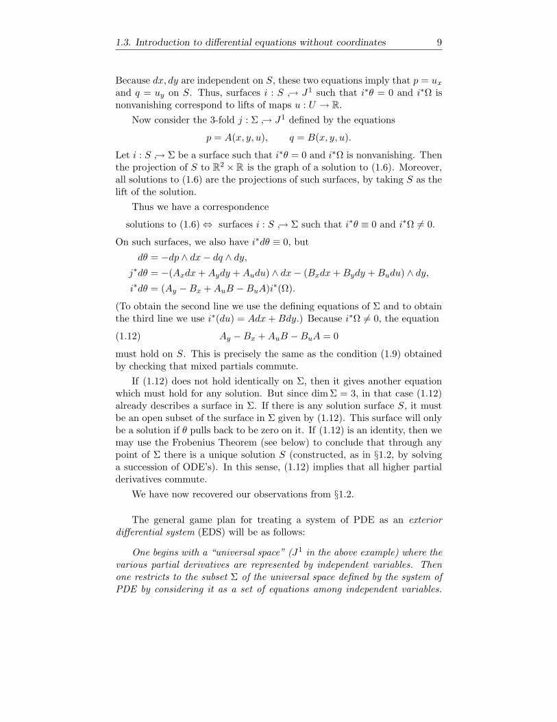
On such surfaces, we also have i∗dθ ≡ 0, but

dθ = −dp ∧ dx− dq ∧ dy,j∗dθ = −(Axdx+Aydy +Audu) ∧ dx− (Bxdx+Bydy +Budu) ∧ dy,i∗dθ = (Ay −Bx +AuB −BuA)i∗(Ω).

(To obtain the second line we use the defining equations of Σ and to obtainthe third line we use i∗(du) = Adx+Bdy.) Because i∗Ω 6= 0, the equation

Ay −Bx +AuB −BuA = 0(1.12)

must hold on S. This is precisely the same as the condition (1.9) obtainedby checking that mixed partials commute.

If (1.12) does not hold identically on Σ, then it gives another equationwhich must hold for any solution. But since dimΣ = 3, in that case (1.12)already describes a surface in Σ. If there is any solution surface S, it mustbe an open subset of the surface in Σ given by (1.12). This surface will onlybe a solution if θ pulls back to be zero on it. If (1.12) is an identity, then wemay use the Frobenius Theorem (see below) to conclude that through anypoint of Σ there is a unique solution S (constructed, as in §1.2, by solvinga succession of ODE’s). In this sense, (1.12) implies that all higher partialderivatives commute.

We have now recovered our observations from §1.2.

The general game plan for treating a system of PDE as an exteriordifferential system (EDS) will be as follows:

One begins with a “universal space” (J1 in the above example) where thevarious partial derivatives are represented by independent variables. Thenone restricts to the subset Σ of the universal space defined by the system ofPDE by considering it as a set of equations among independent variables.

10 1. Moving Frames and Exterior Differential Systems

Solutions to the PDE correspond to submanifolds of Σ on which the vari-ables representing what we want to be partial derivatives actually are partialderivatives. These submanifolds are characterized by the vanishing of certaindifferential forms.

These remarks will be explained in detail in §1.9.Picard’s Theorem revisited. On R2 with coordinates (x, u), consider θ =du−f(x, u)dx. Then there is a one-to-one correspondence between solutionsof the ODE (1.5) and curves c : R → R2 such that c∗(θ) = 0 and c∗(dx) isnonvanishing.

More generally, the flowbox coordinate theorem 1.2.2 implies:

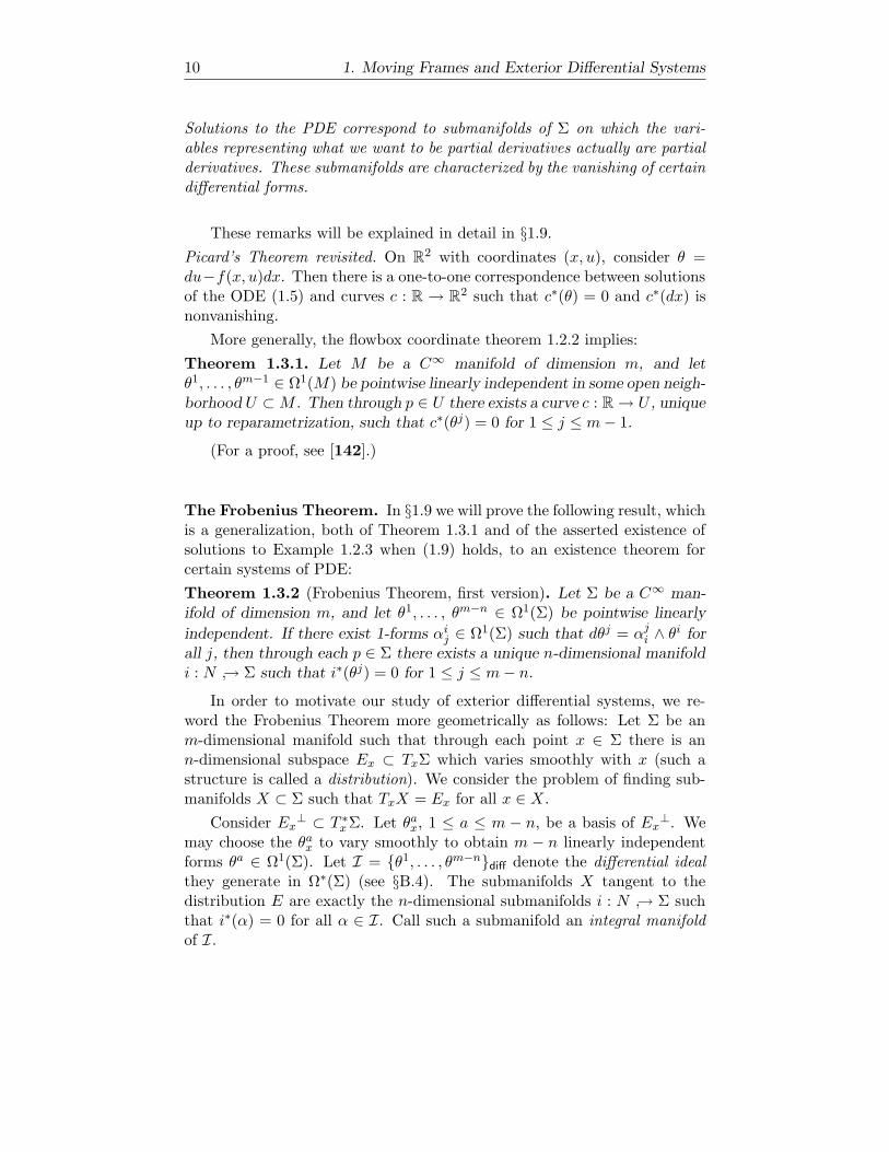
Theorem 1.3.1. Let M be a C∞ manifold of dimension m, and letθ1, . . . , θm−1 ∈ Ω1(M) be pointwise linearly independent in some open neigh-borhood U ⊂M . Then through p ∈ U there exists a curve c : R → U , uniqueup to reparametrization, such that c∗(θj) = 0 for 1 ≤ j ≤ m− 1.

(For a proof, see [142].)

The Frobenius Theorem. In §1.9 we will prove the following result, whichis a generalization, both of Theorem 1.3.1 and of the asserted existence ofsolutions to Example 1.2.3 when (1.9) holds, to an existence theorem forcertain systems of PDE:

Theorem 1.3.2 (Frobenius Theorem, first version). Let Σ be a C∞ man-ifold of dimension m, and let θ1, . . . , θm−n ∈ Ω1(Σ) be pointwise linearly

independent. If there exist 1-forms αij ∈ Ω1(Σ) such that dθj = αji ∧ θi forall j, then through each p ∈ Σ there exists a unique n-dimensional manifoldi : N → Σ such that i∗(θj) = 0 for 1 ≤ j ≤ m− n.

In order to motivate our study of exterior differential systems, we re-word the Frobenius Theorem more geometrically as follows: Let Σ be anm-dimensional manifold such that through each point x ∈ Σ there is ann-dimensional subspace Ex ⊂ TxΣ which varies smoothly with x (such astructure is called a distribution). We consider the problem of finding sub-manifolds X ⊂ Σ such that TxX = Ex for all x ∈ X.

Consider Ex⊥ ⊂ T ∗xΣ. Let θax, 1 ≤ a ≤ m − n, be a basis of Ex

⊥. Wemay choose the θax to vary smoothly to obtain m − n linearly independentforms θa ∈ Ω1(Σ). Let I = θ1, . . . , θm−ndiff denote the differential idealthey generate in Ω∗(Σ) (see §B.4). The submanifolds X tangent to thedistribution E are exactly the n-dimensional submanifolds i : N → Σ suchthat i∗(α) = 0 for all α ∈ I. Call such a submanifold an integral manifoldof I.

1.3. Introduction to differential equations without coordinates 11

To find integral manifolds, we already know that if there are any, theirtangent space at any point x ∈ Σ is already uniquely determined, namelyit is Ex. The question is whether these n-planes can be “fitted together” toobtain an n-dimensional submanifold. This information is contained in thederivatives of the θa’s, which indicate how the n-planes “move” infinitesi-mally.

If we are to have i∗(θa) = 0, we must also have d(i∗θa) = i∗(dθa) = 0. Ifthere is to be an integral manifold through x, or even an n-plane Ex ⊂ TxΣon which α |Ex= 0, ∀α ∈ I, the equations i∗(dθa) = 0 cannot impose anyadditional conditions, i.e., we must have dθa|Ex = 0 because we already havea unique n-plane at each point x ∈ Σ. To recap, for all a we must have

dθa = αa1 ∧ θ1 + . . .+ αam−n ∧ θm−n(1.13)

for some αab ∈ Ω1(Σ), because the forms θax span Ex⊥.

Notation 1.3.3. Suppose I is an ideal and φ and ψ are k-forms. Then wewrite φ ≡ ψmod I if φ = ψ + β for some β ∈ I.

Let θ1, . . . , θm−nalg ⊂ Ω∗(Σ) denote the algebraic ideal generated byθ1, . . . , θm−n (see §B.4). Now (1.13) may be restated as

dθa ≡ 0 mod θ1, . . . , θm−nalg.(1.14)

The Frobenius Theorem states that this necessary condition is also sufficient:

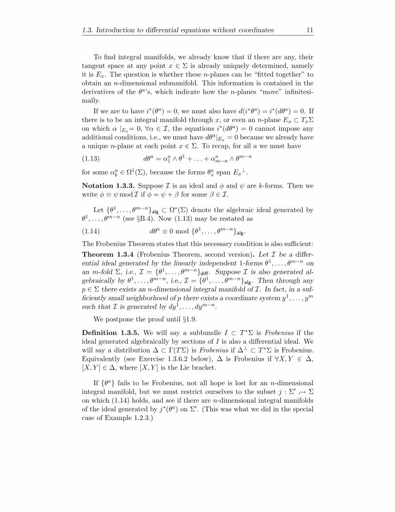
Theorem 1.3.4 (Frobenius Theorem, second version). Let I be a differ-ential ideal generated by the linearly independent 1-forms θ1, . . . , θm−n onan m-fold Σ, i.e., I = θ1, . . . , θm−ndiff. Suppose I is also generated al-gebraically by θ1, . . . , θm−n, i.e., I = θ1, . . . , θm−nalg. Then through anyp ∈ Σ there exists an n-dimensional integral manifold of I. In fact, in a suf-ficiently small neighborhood of p there exists a coordinate system y1, . . . , ym

such that I is generated by dy1, . . . , dym−n.

We postpone the proof until §1.9.Definition 1.3.5. We will say a subbundle I ⊂ T ∗Σ is Frobenius if theideal generated algebraically by sections of I is also a differential ideal. Wewill say a distribution ∆ ⊂ Γ(TΣ) is Frobenius if ∆⊥ ⊂ T ∗Σ is Frobenius.Equivalently (see Exercise 1.3.6.2 below), ∆ is Frobenius if ∀X,Y ∈ ∆,[X,Y ] ∈ ∆, where [X,Y ] is the Lie bracket.

If θa fails to be Frobenius, not all hope is lost for an n-dimensionalintegral manifold, but we must restrict ourselves to the subset j : Σ′ → Σon which (1.14) holds, and see if there are n-dimensional integral manifoldsof the ideal generated by j∗(θa) on Σ′. (This was what we did in the specialcase of Example 1.2.3.)

12 1. Moving Frames and Exterior Differential Systems

Exercises 1.3.6:1. Which of the following ideals are Frobenius?

I1 = dx1, x2dx3 + dx4diffI2 = dx1, x1dx3 + dx4diff

2. Show that the differential forms and vector field conditions for beingFrobenius are equivalent, i.e., ∆ ⊂ Γ(TΣ) satisfies [∆,∆] ⊆ ∆ if and only if∆⊥ ⊂ T ∗Σ satisfies dθ ≡ 0mod∆⊥ for all θ ∈ Γ(∆⊥).3. On R3 let θ = Adx + Bdy + Cdz, where A = A(x, y, z), etc. Assumethe differential ideal generated by θ is Frobenius, and explain how to find afunction f(x, y, z) such that the differential systems θdiff and dfdiff areequivalent.

1.4. Introduction to geometry without coordinates:curves in E2

We will return to our study of surfaces in E3 in Chapter 2. To see how touse moving frames to obtain invariants, we begin with a simpler problem.

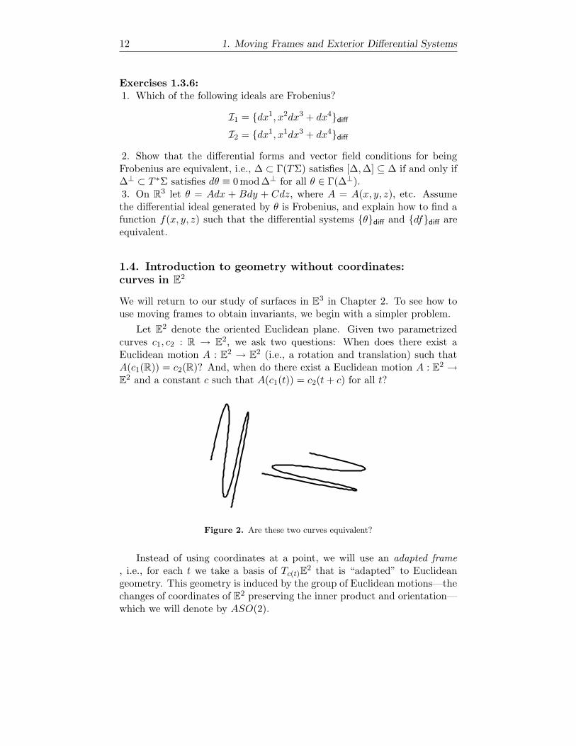
Let E2 denote the oriented Euclidean plane. Given two parametrizedcurves c1, c2 : R → E2, we ask two questions: When does there exist aEuclidean motion A : E2 → E2 (i.e., a rotation and translation) such thatA(c1(R)) = c2(R)? And, when do there exist a Euclidean motion A : E2 →E2 and a constant c such that A(c1(t)) = c2(t+ c) for all t?

Figure 2. Are these two curves equivalent?

Instead of using coordinates at a point, we will use an adapted frame, i.e., for each t we take a basis of Tc(t)E2 that is “adapted” to Euclideangeometry. This geometry is induced by the group of Euclidean motions—thechanges of coordinates of E2 preserving the inner product and orientation—which we will denote by ASO(2).

1.4. Introduction to geometry without coordinates: curves in E2 13

In more detail, the group ASO(2) consists of transformations of the form(x1

x2

)7→(t1

t2

)+R

(x1

x2

),(1.15)

where R ∈ SO(2) is a rotation matrix. It can be represented as a matrixLie group by writing

ASO(2) =

M ∈ GL(3,R)

∣∣∣∣M =

(1 0t R

), t ∈ R2, R ∈ SO(2)

.(1.16)

Then its action on E2 is given by x 7→Mx, where we represent points in E2

by x = t(1 x1 x2

).

We may define a mapping from ASO(2) to E2 by(1 0x R

)7→ x =

(x1x2

),(1.17)

which takes each group element to the image of the origin under the trans-formation (1.15). The fiber of this map over every point is a left coset ofSO(2) ⊂ ASO(2), so E2, as a manifold, is the quotient ASO(2)/SO(2). Fur-thermore, ASO(2) may be identified with the bundle of oriented orthonormalbases of E2 by identifying the columns of the rotation matrix R = (e1, e2)with an oriented orthonormal basis of TxE2, where x is the basepoint givenby (1.17). (Here we use the fact that for a vector space V , we may identifyV with TxV for any x ∈ V .)

Returning to the curve c(t), we choose an oriented orthonormal basisof Tc(t)E2 as follows: A natural element of Tc(t)E2 is c′(t), but this maynot be of unit length. So, we take e1(t) = c′(t)/|c′(t)|, and this choice alsodetermines e2(t). Of course, to do this we must assume that the curve isregular:

Definition 1.4.1. A curve c(t) is said to be regular if c′(t) never vanishes.More generally, a map f : M → N between differentiable manifolds isregular if df is everywhere defined and of rank equal to dimM .

What have we done? We have constructed a map to the Lie groupASO(2) as follows:

C : R → ASO(2),

t 7→(

1 0c(t) (e1(t), e2(t))

).

We will obtain differential invariants of our curve by differentiating thismapping, and taking combinations of the derivatives that are invariant underEuclidean changes of coordinates.

14 1. Moving Frames and Exterior Differential Systems

Consider v(t) = |c′(t)|, called the speed of the curve. It is invariant underEuclidean motions and thus is a differential invariant. However, it is onlyan invariant of the mapping, not of the image curve (see Exercise 1.4.2.2).The speed measures how much (internal) distance is being distorted underthe mapping c.

Consider de1dt . We must have de1

dt = λ(t)e2(t) for some function λ(t) be-cause |e1(t)| ≡ 1 (see Exercise 1.4.2.1 below). Thus λ(t) is a differential in-variant, but it again depends on the parametrization of the curve. To deter-mine an invariant of the image alone, we let c(t) be another parametrization

of the same curve. We calculate that λ(t) = v(t)v(t)λ(t), so we set κ(t) = λ(t)

v(t) .

This κ(t), called the curvature of the curve, measures how much c is in-finitesimally moving away from its tangent line at c(t).

A necessary condition for two curves c, c to have equivalent images is thatthere exists a diffeomorphism ψ : R → R such that κ(t) = κ(ψ(t)). It willfollow from Corollary 1.6.13 that the images of curves are locally classifiedup to congruence by their curvature functions, and that parametrized curvesare locally classified by κ, v.

Exercises 1.4.2:1. Let V be a vector space with a nondegenerate inner product 〈, 〉. Letv(t) be a curve in V such that F (t) := 〈v(t), v(t)〉 is constant. Show thatv′(t) ⊥ v(t) for all t. Show the converse is also true.

2. Suppose that c is regular. Let s(t) =∫ t0 |c′(τ)|dτ and consider c paramet-

rized by s instead of t. Since s gives the length of the image of c : [0, s]→ E2,s is called an arclength parameter. Show that in this preferred parametriza-tion, κ(s) = |de1ds |.3. Show that κ(t) is constant iff the curve is an open subset of a line (ifκ = 0) or circle of radius 1

κ .4. Let c(t) = (x(t), y(t)) be given in coordinates. Calculate κ(t) in termsof x(t), y(t) and their derivatives.5. Calculate the function κ(t) for an ellipse. Characterize the points on theellipse where the maximum and minimum values of κ(t) occur.6. Can κ(t) be unbounded if c(t) is the graph of a polynomial?

Exercise 1.4.3 (Osculating circles):(a) Calculate the equation of a circle passing through three points in theplane.(b) Calculate the equation of a circle passing through two points in theplane and having a given tangent line at one of the points.

Parts (a) and (b) may be skipped; the exercise proper starts here:

(c) Show that for any curve c ⊂ E2, at each point x ∈ c one can define anosculating circle by taking the limit of the circle through the three points

1.5. Submanifolds of homogeneous spaces 15

c(t), c(t1), c(t2) as t1, t2 → t. (A line is defined to be a circle of infiniteradius.)(d) Show that one gets the same circle if one takes the limit as t → t1 ofthe circle through c(t), c(t1) that has tangent line at c(t) parallel to c′(t).(e) Show that the radius of the osculating circle is 1/κ(t).(f) Show that if κ(t) is monotone, then the osculating circles are nested.

1.5. Submanifolds of homogeneous spaces

Using the machinery we develop in this section and §1.6, we will answer thequestions about curves in E2 posed at the beginning of §1.4. The quotientE2 = ASO(2)/SO(2) is an example of a homogeneous space, and our answerswill follow from a general study of classifying maps into homogeneous spaces.

Definition 1.5.1. Let G be a Lie group, H a closed Lie subgroup, and G/Hthe set of left cosets of H. Then G/H is naturally a differentiable manifoldwith the induced differentiable structure coming from the quotient map (see[77], Theorem II.3.2). The space G/H is called a homogeneous space.

Definition 1.5.2 (Left and right actions). Let G be a group that acts on aset X by x 7→ σ(g)(x). Then σ is called a left action if σ(a) σ(b) = σ(ab),or a right action if σ(a) σ(b) = σ(ba),

For example, the action of G on itself by left-multiplication is a leftaction, while left-multiplication by g−1 is a right action.

A homogeneous space G/H has a natural (left) G-action on it; the sub-group stabilizing [e] is H, and the stabilizer of any point is conjugate toH. Conversely, a manifold X is a homogeneous space if it admits a smoothtransitive action by a Lie group G. If H is the isotropy group of a pointx0 ∈ X, then X ' G/H, and x0 corresponds to [e] ∈ G/H, the coset ofthe identity element. (See [77, 142] for additional facts about homogeneousspaces.)

In the spirit of Klein’s Erlanger Programm (see [76, 92] for historicalaccounts), we will consider G as the group of motions of G/H. We willstudy the geometry of submanifolds M ⊂ G/H, where two submanifoldsM,M ′ ⊂ G/H will be considered equivalent if there exists a g ∈ G such thatg(M) =M ′.

To determine necessary conditions for equivalence we will find differentialinvariants as we did in §1.1 and §1.4. (Note that we need to specify whetherwe are interested in invariants of a mapping or just of the image.) Afterfinding invariants, we will then interpret them as we did in the exercises in§1.4.

Chapter 2

Euclidean Geometryand RiemannianGeometry

In this chapter we return to the study of surfaces in Euclidean space E3 =ASO(3)/SO(3). Our goal is not just to understand Euclidean geometry, butto develop techniques for solving equivalence problems for submanifolds ofarbitrary homogeneous spaces. We begin with the problem of determiningif two surfaces in E3 are locally equivalent up to a Euclidean motion. Moreprecisely, given two immersions f, f : U → E3, where U is a domain inR2, when do there exist a local diffeomorphism φ : U → U and a fixedA ∈ ASO(3) such that f φ = A f? Motivated by our results on curvesin Chapter 1, we first try to find a complete set of Euclidean differentialinvariants for surfaces in E3, i.e., functions I1, . . . , Ir that are defined interms of the derivatives of the parametrization of a surface, with the propertythat f(U) differs from f(U) by a Euclidean motion if and only if (f φ)∗Ij =f∗Ij for 1 ≤ j ≤ r.

In §2.1 we derive the Euclidean differential invariants Gauss curvatureK and mean curvature H using moving frames. Unlike with curves in E3,for surfaces in E3 there is not always a unique lift to ASO(3), and we are ledto define the space of adapted frames. (Our discussion of adapted frames forsurfaces in E3 is later generalized to higher dimensions and codimensions in§2.5.) We calculate the functions H,K for two classical classes of surfacesin §2.2; developable surfaces and surfaces of revolution, and discuss basicproperties of these surfaces.

35

36 2. Euclidean Geometry and Riemannian Geometry

Scalar-valued differential invariants turn out to be insufficient (or at leastnot convenient) for studying equivalence of surfaces and higher-dimensionalsubmanifolds, and we are led to introduce vector bundle valued invariants.This study is motivated in §2.4 and carried out in §2.5, resulting in thedefinitions of the first and second fundamental forms, I and II. In §2.5 wealso interpret II and Gauss curvature, define the Gauss map and derive theGauss equation for surfaces.

Relations between intrinsic and extrinsic geometry of submanifolds ofEuclidean space are taken up in §2.6, where we prove Gauss’s theoremaegregium, derive the Codazzi equation, discuss frames for C∞ manifolds andRiemannian manifolds, and prove the fundamental lemma of Riemanniangeometry. We include many exercises about connections, curvature, theLaplacian, isothermal coordinates and the like. We conclude the sectionwith the fundamental theorem for hypersurfaces.

In §2.7 and §2.8 we discuss two topics we will need later on, space formsand curves on surfaces. In §2.9 we discuss and prove the Gauss-Bonnet andPoincare-Hopf theorems. We conclude this chapter with a discussion of non-orthonormal frames in §2.10, which enables us to finally prove the formula(1.3) and show that surfaces with H identically zero are minimal surfaces.

The geometry of surfaces in E3 is studied further in §3.1 and throughoutChapters 5–7. Riemannian geometry is discussed further in Chapter 8.

2.1. Gauss and mean curvature via frames

Guided by Cartan’s Theorem 1.6.11, we begin our search for differentialinvariants of immersed surfaces f : U 2 → E3 by trying to find a lift F : U →ASO(3) which is adapted to the geometry of M = f(U). The most naıvelift would be to take

F (p) =

(1 0

f(p) Id

).

Any other lift F is of the form

F = F

(1 00 R

)

for some map R : U → SO(3).

Let x = f(p); then TxE3 has distinguished subspaces, namely f∗(TpU)and its orthogonal complement. We use our rotational freedom to adaptto this situation by requiring that e3 always be normal to the surface, orequivalently that e1, e2 span TxM . This is analogous to our choice ofcoordinates at our preferred point in Chapter 1, but is more powerful sinceit works on an open set of points in U .

Chapter 3

Projective Geometry

This chapter may be considered as an update to the paper of Griffiths andHarris [69], which began a synthesis of modern algebraic geometry and mov-ing frames techniques. Other than the first three sections, it may be skippedby readers anxious to arrive at the Cartan-Kahler Theorem. An earlier ver-sion of this chapter, containing more algebraic results than presented here,constituted the monograph [107].

We study the local geometry of submanifolds of projective space andapplications to algebraic geometry. We begin in §3.1 with a discussion ofGrassmannians, one of the most important classes of manifolds in all of ge-ometry, and some uses of Grassmannians in Euclidean geometry. We definethe Euclidean and projective Gauss maps. We then describe moving framesfor submanifolds of projective space and define the projective second funda-mental form in §3.2. In §3.3 we give some basic definitions from algebraicgeometry. We give examples of homogeneous algebraic varieties and explainseveral constructions of auxiliary varieties from a given variety X ⊂ PV :the secant variety σ(X), the tangential variety τ(X) and the dual varietyX∗. In §3.4 we describe the basic properties of varieties with degenerateGauss maps and classify the surface case. We return in §§3.5–3.7 to discussmoving frames and differential invariants in more detail, with plenty of ho-mogeneous examples in §3.6. We discuss osculating hypersurfaces and provehigher-order Bertini theorems in §3.7.

In §3.8 and §3.9, we apply our machinery respectively to study uniruledvarieties and to characterize quadric hypersurfaces (Fubini’s Theorem). Va-rieties with degenerate duals and associated varieties are discussed in §3.10and §3.11 respectively. We prove the bounds of Zak and Landman on thedual defect from our differential-geometric perspective. In §3.12 we study

71

72 3. Projective Geometry

varieties with degenerate Gauss images in further detail. In §3.14 we stateand prove rank restriction theorems: we show that the projective second fun-damental form has certain genericity properties in small codimension if X isnot too singular. We describe how to calculate dimσ(X) and dim τ(X) in-finitesimally, and state the Fulton-Hansen Theorem relating tangential andsecant varieties. In §3.13 we state Zak’s theorem classifying Severi varieties,the smooth varieties of minimal codimension having secant defects. Section§3.15 is dedicated to the proof of Zak’s theorem. In §3.16 we generalizeFubini’s Theorem to higher codimension, and finally in §3.17 we discussapplications to the study of complete intersections.

In this chapter, when we work over the complex numbers, all tangent,cotangent, etc., spaces are the holomorphic tangent, cotangent, etc., spaces(see Appendix C). We will generally use X to denote an algebraic varietyand M to denote a complex manifold.

Throughout this chapter we often commit the following abuse of nota-tion: We omit the in symmetric products and the ⊗ when the product isclear from the context. For example, we will often write ωα0 eα for ωα0 ⊗eα.

3.1. Grassmannians

In projective geometry, Grassmannians play a central role, so we begin witha study of Grassmannians and the Plucker embedding. We also give appli-cations to Euclidean geometry.

We fix index ranges 1 ≤ i, j ≤ k, and k+ 1 ≤ s, t, u ≤ n for this section.

Let V be a vector space over R or C and let G(k, V ) denote the Grass-mannian of k-planes that pass through the origin in V . To specify a k-planeE, it is sufficient to specify a basis v1, . . . , vk of E. We continue our nota-tional convention that v1, . . . , vk denotes the span of the vectors v1, . . . , vk.After fixing a reference basis, we identify GL(V ) with the set of bases forV , and define a map

π : GL(V )→ G(k, V ),

(e1, . . . , en) 7→ e1, . . . , ek,If we let e1, . . . , en denote the standard basis of V , i.e., eA is a column vectorwith a 1 in the A-th slot and zeros elsewhere, the fiber of this mapping overπ(Id) = e1, . . . , ek, is the subgroup

Pk =

g =

(gij gis0 gts

)| det(g) 6= 0

⊂ GL(V ).

More generally, for g ∈ GL(V ), π−1(π(g)) = gPkg−1.

Of particular importance is projective space PV = G(1, V ), the spaceof all lines through the origin in V . We define a line in PV to be the

Chapter 4

Cartan-Kahler I:Linear Algebra andConstant-CoefficientHomogeneous Systems

We have seen that differentiating the forms that generate an exterior dif-ferential system often reveals additional conditions that integral manifoldsmust satisfy (e.g., the Gauss and Codazzi equations for a surface in Eucli-dean space). The conditions are consequences of the fact that mixed partialsmust commute. What we did not see was a way of telling when one has dif-ferentiated enough to find all hidden conditions. We do know the answerin two cases: If a system is in Cauchy-Kowalevski form there are no extraconditions. In the case of the Frobenius Theorem, if the system passes afirst-order test, then there are no extra conditions.

What will emerge over the next few chapters is a test, called Cartan’sTest, that will tell us when we have differentiated enough.

The general version of Cartan’s Test is described in Chapter 7. For agiven integral element E ∈ Vn(I)x of an exterior differential system I ona manifold Σ, it guarantees existence of an integral manifold to the systemwith tangent plane E if E passes the test.

In Chapter 5, we present a version of Cartan’s Test valid for a classof exterior differential systems with independence condition called linearPfaffian systems. These are systems that are generated by 1-forms andhave the additional property that the variety of integral elements through a

143

144 4. Constant-Coefficient Homogeneous Systems

point x ∈ Σ is an affine space. The class of linear Pfaffian systems includesall systems of PDE expressed as exterior differential systems on jet spaces.One way in which a linear Pfaffian system is simpler than a general EDS isthat an integral element E ∈ Vn(I,Ω)x passes Cartan’s Test iff all integralelements at x do.

In this chapter we study first-order, constant-coefficient, homogeneoussystems of PDE for analytic maps f : V →W expressed in terms of tableaux.We derive Cartan’s Test for this class of systems, which determines if theinitial data one might naıvely hope to specify (based on counting equations)actually determines a solution.

We dedicate an entire chapter to such a restrictive class of EDS becauseat each point of a manifold Σ with a linear Pfaffian system there is a naturallydefined tableau, and the system passes Cartan’s Test for linear Pfaffiansystems at a point x ∈ Σ if and only if its associated tableau does and thetorsion of the system (defined in Chapter 5) vanishes at x.

In analogy with the inverse function theorem, Cartan’s Test for linearPfaffian systems (and even in its most general form) implies that if the linearalgebra at the infinitesimal level works out right, the rest follows. What wedo in this chapter is determine what it takes to get the linear algebra towork out right.

Throughout this chapter, V is an n-dimensional vector space, and Wis an s-dimensional vector space. We use the index ranges 1 ≤ i, j, k ≤ n,1 ≤ a, b, c ≤ s. V has the basis v1, . . . , vn and V ∗ the corresponding dualbasis v1, . . . , vn; W has basis w1, . . . , ws and W

∗ the dual basis w1, . . . , ws.

4.1. Tableaux

Let x = xivi, u = uawa denote elements of V and W respectively. We willconsider (x1, . . . , xn), respectively (u1, . . . , un), as coordinate functions onV and W respectively. Any first-order, constant-coefficient, homogeneoussystem of PDE for maps f : V →W is given in coordinates by equations

Bria

∂ua

∂xi= 0, 1 ≤ r ≤ R,(4.1)

where the Bria are constants. For example, the Cauchy-Riemann system

u1x1 − u2x2 = 0, u1x2 + u2x1 = 0 has B111 = 1, B12

2 = −1, B121 = 0, B11

2 = 0,

B212 = 1, B22

1 = 1, B211 = 0 and B22

2 = 0.

Chapter 5

Cartan-Kahler II:The Cartan Algorithmfor Linear PfaffianSystems

We now generalize the test from Chapter 4 to a test valid for a large class ofexterior differential systems called linear Pfaffian systems, which are definedin §5.1. In §§5.2–5.4 we present three examples of linear Pfaffian systems thatlead us to Cartan’s algorithm and the definitions of torsion and prolongation,all of which are given in §5.5. For easy reference, we give a summary andflowchart of the algorithm in §5.6. Additional aspects of the theory, includ-ing characteristic hyperplanes, Spencer cohomology and the Goldschmidtversion of the Cartan-Kahler Theorem, are given in §5.7. In the remainderof the chapter we give numerous examples, beginning with elementary prob-lems coming mostly from surface theory in §5.8, then an example motivatedby variation of Hodge structure in §5.9, then the Cartan-Janet Isometric Im-mersion Theorem in §5.10, followed by a discussion of isometric embeddingsof space forms in §5.11 and concluding with a discussion of calibrations andcalibrated submanifolds in §5.12.

5.1. Linear Pfaffian systems

Recall that a Pfaffian system on a manifold Σ is an exterior differentialsystem generated by 1-forms, i.e., I = θadiff, θa ∈ Ω1(Σ), 1 ≤ a ≤ s. IfΩ = ω1 ∧ . . . ∧ ωn represents an independence condition, let J := θa, ωi

163

164 5. The Cartan Algorithm for Linear Pfaffian Systems

and I := θa. We will often use J to indicate the independence conditionin this chapter, and refer to the system as (I, J).

Definition 5.1.1. (I, J) is a linear Pfaffian system if dθa ≡ 0 mod J forall 1 ≤ a ≤ s.

Exercise 5.1.2: Let (I, J) be a linear Pfaffian system as above. Let πε,1 ≤ ε ≤ dimΣ − n − s, be a collection of 1-forms such that T ∗Σ is locallyspanned by θa, ωi, πε. Show that there exist functions Aaεi, T

aij defined on Σ

such that

dθa ≡ Aaεiπε ∧ ωi + T aijω

i ∧ ωj mod I.(5.1)

Example 5.1.3. The canonical contact system on J2(R2,R2) is a linearPfaffian system because

d(du− p11dx− p12dy) = −dp11 ∧ dx− dp12 ∧ dy≡ 0moddx, dy, du− p11dx− p12dy, dv − p21dx− p22dy,

d(dv − p21dx− p22dy) = −dp21 ∧ dx− dp22 ∧ dy≡ 0moddx, dy, du− p11dx− p12dy, dv − p21dx− p22dy,

and the same calculation shows that the pullback of this system to anysubmanifold Σ ⊂ J2(R2,R2) is linear Pfaffian. More generally, we have

Example 5.1.4. Any system of PDE expressed as the pullback of the con-tact system on Jk(M,N) to a subset Σ is a linear Pfaffian system. If M haslocal coordinates (x1, . . . , xn) and N has local coordinates (u1, . . . , us), thenJk = Jk(M,N) has local coordinates (xi, ua, pai , p

aL), where L = (l1, . . . , lp)

is a symmetric multi-index of length p ≤ k−1. In these coordinates, the con-tact system I is θa = dua−pai dxi, θaL = dpaL−paLjdxj, and J = θa, θaL, dxi.On Jk(M,N),

dθa = −dpaj ∧ dxj

dθaL = −dpaLj ∧ dxj

≡ 0 mod J,

and these equations continue to hold when we restrict to any subset Σ ⊂ J k.

Example 5.1.5. On R6, let θ = y1dy2 + y3dy4 + y5dx, let I = θ andJ = θ, dx. Then

dθ = dy1 ∧ dy2 + dy3 ∧ dy4 + dy5 ∧ dx

≡ (dy3 − y3

y1dy1) ∧ dy4modθ, dx.

In this case, (I, J) is not a linear Pfaffian system.

178 5. The Cartan Algorithm for Linear Pfaffian Systems

Rename Σ′ as Σ -

Input:linear Pfaffian system

(I, J) on Σ;calculate dImod I

¾

Prolong to a componentof Vn(I,Ω) ⊂ Gn(TΣ);rename component as Σ,

canonical systembecomes (I, J)6

N´

´´

´´

´

QQQQ

QQQQ

Is Σ′ empty?

?´

´´

´´

´

QQQQ

QQQQ

Is [T ] = 0? -Y

6N

´´

´´

´´

´´

QQQQQ

QQQQQ

Is tableauinvolutive?

?

Y

Done:there are no

integral manifolds

?N

Restrict to Σ′ ⊂ Σdefined by [T ] = 0and Ω |Σ′ 6= 0

QQ

QQ

QQk

?

Y

Done:local existence ofintegral manifolds

Figure 1. Our final flowchart.

Warning: Where the algorithm ends up (i.e., in which “Done” box inthe flowchart) may depend on the component one is working on.

Summary. Let (I, J) be a linear Pfaffian system on Σ. We summarizeCartan’s algorithm:

(1) Take a local coframing of Σ adapted to the filtration I ⊂ J ⊂ T ∗Σ.Let x ∈ Σ be a general point. Let V ∗ = (J/I)x, W

∗ = Ix, andlet vi = ωix, w

a = θax and vi, wa be the corresponding dual basisvectors.

(2) Calculate dθa; since the system is linear, these are of the form

dθa ≡ Aaεiπε ∧ ωi + T aijω

i ∧ ωj mod I.

Define the tableau at x by

A = Ax := Aaεivi⊗wa ⊆ V ∗⊗W | 1 ≤ ε ≤ r ⊆W⊗V ∗.Let δ denote the natural skew-symmetrization map δ : W ⊗V ∗⊗V ∗ →W⊗Λ2V ∗ and let

H0,2(A) :=W⊗Λ2V ∗/δ(A⊗V ∗).The torsion of (I, J) at x is

[T ]x := [T aijwa⊗vi ∧ vj ] ∈ H0,2(A).

(3) If [T ]x 6= 0, then start again on Σ′ ⊂ Σ defined by the equations[T ] = 0, with the additional requirement that J/I has rank n over

5.7. Additional remarks on the theory 179

Σ′. Since the additional requirement is a transversality condition,it will be generically satisfied as long as dimΣ′ ≥ n. In practiceone works infinitesimally, using the equations d[T ] = 0, and checkswhat relations d[T ] ≡ 0 mod I imposes on the forms πε used before.

(4) Assume [T ]x = 0. Let Ak := A ∩ (spanvk+1, . . . , vn⊗W ). Let

A(1) := (A⊗V ∗) ∩ (W⊗S2V ∗), the prolongation of the tableau A.Then

dimA(1) ≤ dimA+ dimA1 + . . .+ dimAn−1

and A is involutive if equality holds.Warning: One can fail to obtain equality even when the system

is involutive if the bases were not chosen sufficiently generically.In practice, one does the calculation with a natural, but perhapsnongeneric basis and takes linear combinations of the columns ofA to obtain genericity. If the bases are generic, then equality holdsiff A is involutive.

When doing calculations, it is convenient to define the char-acters sk by s1 + . . . + sk = dimA − dimAk, in which case theinequality becomes dimA(1) ≤ s1 + 2s2 + . . .+ nsn. If sp 6= 0 andsp+1 = 0, then sp is called the character of the tableau and p theCartan integer. If A is involutive, then the Cartan-Kahler Theo-rem applies, and one has local integral manifolds depending on spfunctions of p variables.

(5) If A is not involutive, prolong, i.e., start over on the pullback of thecanonical system on the Grassmann bundle to the space of integralelements. In calculations this amounts to adding the elements ofA(1) as independent variables, and adding differential forms θai :=

Aaεiπε − paijωj to the ideal, where paijv

ivj⊗wa ∈ A(1).

5.7. Additional remarks on the theory

Another interpretation of A(1). We saw in Chapter 4 that for a constant-coefficient, first-order, homogeneous system defined by a tableau A, theprolongation A(1) is the space of admissible second-order terms paijx

ixj in apower series solution of the system. This was because the constants paij had

to satisfy paijwa⊗vi⊗vj ∈ A(1).

The following proposition, which is useful for computing A(1), is thegeneralization of this observation to linear Pfaffian systems:

Proposition 5.7.1. After fixing x ∈ Σ and a particular choice of 1-formsπai mod I satisfying dθa ≡ πai ∧ ωimod I, A(1) may be identified with thespace of 1-forms πai mod I satisfying dθa ≡ πai ∧ωimod I, as follows: any such

Chapter 6

Applications to PDE

Introduction. Consider the well-known closed-form solution of the waveequation utt − c2uxx = 0 due to d’Alembert:

u(x, t) = f(x+ ct) + g(x− ct),(6.1)

where f and g are arbitrary C2 functions. It is rare that all solutions ofa given PDE are obtained by a single formula (especially, one which doesnot involve integration). The key to obtaining the d’Alembert solution is torewrite the equation in “characteristic coordinates” η = x + ct, ξ = x − ct,yielding uηξ = 0. By integrating in η or in ξ, we get

uη = F (η), uξ = G(ξ),

where F and G are independent arbitrary functions; then (6.1) follows byanother integration. For which other PDE do such solution formulas exist?And, how can we find them in a systematic way?

In this chapter we study invariants of exterior differential systems thataid in constructing integral manifolds, and we apply these to the study offirst and second-order partial differential equations, and classical surfacetheory. (For second-order PDE, we will restrict attention to equations forone function of two variables.) All functions and forms are assumed to besmooth.

In §6.1 we define symmetry vector fields and in particular Cauchy char-acteristic vector fields for EDS. We discuss the general properties of Cauchycharacteristics, and use them to recover the classical result that any first-order PDE can be solved using ODE methods. In §6.2 we define theMonge characteristic systems associated to second-order PDE, and discusshyperbolic exterior differential systems. In §6.3 we discuss a systematic

203

204 6. Applications to PDE

method, called Darboux’s method, which helps uncover solution formulaslike d’Alembert’s (when they exist), and more generally determines when agiven PDE is solvable by ODE methods. We also define the derived systemsassociated to a Pfaffian system.

In §6.4 we treat Monge-Ampere systems, focusing on several geometricexamples. We show how solutions of the sine-Gordon equation enable us toexplicitly parametrize surfaces in E3 with constant negative Gauss curva-ture. We show how consideration of complex characteristics, for equationsfor minimal surfaces and for surfaces of constant mean curvature (CMC),leads to solutions for these equations in terms of holomorphic data. In par-ticular, we derive the Weierstrass representation for minimal surfaces andshow that any CMC surface has a one-parameter family of non-congruentdeformations.

In §6.5 we discuss integrable extensions and Backlund transformations.Examples discussed include the Cole-Hopf and Miura transformations, theKdV equation, and Backlund’s original transformation for pseudosphericalsurfaces. We also prove Theorem 6.5.14, relating Backlund transformationsto Darboux-integrability.

6.1. Symmetries and Cauchy characteristics

Infinitesimal symmetries. One of Lie’s contributions to the theory ofordinary differential equations was to put the various solution methods forspecial kinds of equations in a uniform context, based on infinitesimal sym-metries of the equation—i.e., vector fields whose flows take solutions tosolutions. This generalizes to EDS when we let the vector fields act ondifferential forms via the Lie derivative operator L (see Appendix B):

Definition 6.1.1. Let I be an EDS on Σ. A vector field v ∈ Γ(TΣ) is an(infinitesimal) symmetry of I if Lvψ ∈ I for all ψ ∈ I.

Exercises 6.1.2:1. The Lie bracket of any two symmetries is a symmetry; thus, symmetriesof a given EDS form a Lie algebra. 2. To show that v is a symmetry, it suffices to check the condition in Defi-nition 6.1.1 on a set of forms which generate I differentially. 3. Let I be the Pfaffian system generated by the contact form θ = dy−zdxon R3. Verify that

v = f∂

∂x+ g

∂

∂y+ (gx + zgy − zfx − z2fy)

∂

∂z,(6.2)

for any functions f(x, y), g(x, y), is a symmetry. Then, find the most generalsymmetry vector field for I.

Chapter 7

Cartan-Kahler III:The General Case

In this chapter we will discuss the Cartan-Kahler Theorem, which guaranteesthe existence of integral manifolds for arbitrary exterior differential systemsin involution. This theorem is a generalization of the Cauchy-KowalevskiTheorem (see Appendix D), which gives conditions under which an analyticsystem of partial differential equations has an analytic solution (definedin the neighborhood of a given point) satisfying a Cauchy problem, i.e.,initial data for the solution specified along a hypersurface in the domain.Similarly, the “initial data” for the Cartan-Kahler Theorem is an integralmanifold of dimension n, which we want to extend to an integral manifoldof dimension n + 1. In Cauchy-Kowalevski, the equations are assumed tobe of a special form, which has the feature that no conflicts arise when onedifferentiates them and equates mixed partials. The condition of involutivityis a generalization of this, guaranteeing that no new integrability conditionsarise when one looks at the equations that higher jets of solutions mustsatisfy.

The reader may wonder why one bothers to consider any exterior dif-ferential systems other than linear Pfaffian systems. For, as remarked inChapter 5, the prolongation of any exterior differential system is a linearPfaffian system, so theoretically it is sufficient to work with such systems.However, in practice it is generally better to work on the smallest spacepossible. In fact, certain spectacular successes of the EDS machinery wereobtained by cleverly rephrasing systems that were naıvely expressed as lin-ear Pfaffian systems as systems involving generators of higher degree on asmaller manifold. One elementary example of this is the study of linear

243

244 7. Cartan-Kahler III: The General Case

Weingarten surfaces (see §6.4); a more complex example is Bryant’s proofof the existence of manifolds with holonomy G2 [17].

We begin this chapter with a more detailed study of the space of integralelements of an EDS. Before proving the full Cartan-Kahler Theorem, in §7.2we give an example that shows how one can use the Cauchy-Kowalevski The-orem to construct triply orthogonal systems of surfaces. (This also serves asa model for the proof in §7.3.) In §7.4 we discuss Cartan’s Test, a procedureby which one can test for involution, and which was already described inChapter 5 for the special case of linear Pfaffian systems. Then in §7.5 wegive a few more examples that illustrate how one applies Cartan’s Test inthe non-Pfaffian case.

7.1. Integral elements and polar spaces

Suppose I is an exterior differential system on Σ; we will assume that Icontains no 0-forms (otherwise, we could restrict to subsets of Σ on whichthe 0-forms vanish). Recall from §1.9 that Vn(I)p ⊂ G(n, TpΣ) denotes thespace of n-dimensional integral elements in TpΣ and Vn = Vn(I) ⊂ Gn(TΣ)the space of all n-dimensional integral elements. In this chapter we willobtain a criterion that guarantees that a given E ∈ Vn(I)p is tangent toan integral manifold. We think of this as “extending” (p,E) to an integralmanifold.

Coordinates on Gn(TΣ). To study the equations that define Vn, we uselocal coordinates on the Grassmann bundle Gn(TΣ). Given E ∈ Gn(TpΣ),there are coordinates x1, . . . , xn and y1, . . . , ys on Σ near p such that E isspanned by the vectors ∂/∂xi. By continuity, there is a neighborhood of E

in Gn(TΣ) consisting of n-planes E such that dx1∧· · ·∧dxn|E6= 0. For each

E, there are numbers pai such that dya|E= pai dx

i|E; these pai , along with the

x’s and y’s, form a local coordinate system on Gn(TΣ).

Recall from Exercise 1.9.4 that E ∈ Vn(I) if and only if every ψ ∈ Invanishes on E. Each such ψ has some expression

ψ =∑

I,J

fIJ dyI ∧ dxJ ,

where I and J are multi-indices with components in increasing order, suchthat |I| + |J | = n, and the fIJ are smooth functions on Σ. Then ψ|

E=

Fψdx1 ∧ . . . ∧ dxn|

E, where the Fψ are polynomials in the pai , given by

F =∑

I,J,L

fI,J (x, y)pi1l1. . . piklkdx

L ∧ dxJ ,

Chapter 8

Geometric Structuresand Connections

We study the equivalence problem for geometric structures. That is, giventwo geometric structures (e.g., pairs of Riemannian manifolds, pairs of man-ifolds equipped with foliations, etc.), we wish to find differential invariantsthat determine existence of a local diffeomorphism preserving the geometricstructures. We begin in §8.1 with two examples, 3-webs in the plane and Rie-mannian geometry, before concluding the section by defining G-structures.In order to find differential invariants, we will need to take derivatives insome geometrically meaningful way, and we spend some time (§§8.2–8.4)figuring out just how to do this. In §8.3 we define connections on coframebundles and briefly discuss a general algorithm for finding differential in-variants of G-structures. In §8.5 we define and discuss the holonomy ofa Riemannian manifold. In §8.6 we present an extended example of theequivalence problem, finding the differential invariants of a path geometry.Finally, in §8.7 we discuss generalizations of G-structures and recent workinvolving these generalizations.

8.1. G-structures

In this section we present two examples of G-structures and then give aformal definition.

First example: 3-webs in R2.

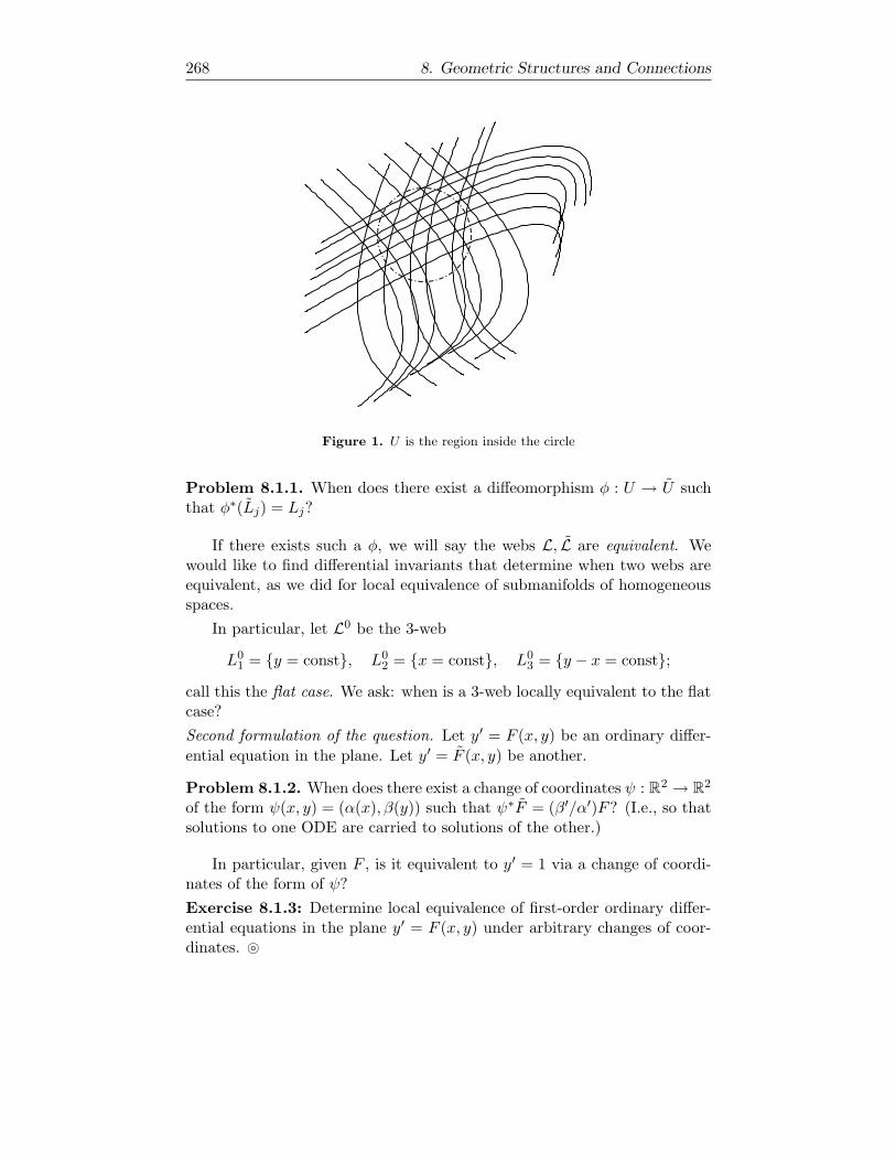
First formulation of the question. Let L = L1, L2, L3 be a collection ofthree pairwise transverse foliations of an open subset U ⊆ R2. Such astructure is called a 3-web; see Figure 1.

Let L = L1, L2, L3 be another 3-web on an open subset U ⊂ R2.

267

268 8. Geometric Structures and Connections

Figure 1. U is the region inside the circle

Problem 8.1.1. When does there exist a diffeomorphism φ : U → U suchthat φ∗(Lj) = Lj?

If there exists such a φ, we will say the webs L, L are equivalent. Wewould like to find differential invariants that determine when two webs areequivalent, as we did for local equivalence of submanifolds of homogeneousspaces.

In particular, let L0 be the 3-web

L01 = y = const, L0

2 = x = const, L03 = y − x = const;

call this the flat case. We ask: when is a 3-web locally equivalent to the flatcase?

Second formulation of the question. Let y′ = F (x, y) be an ordinary differ-

ential equation in the plane. Let y′ = F (x, y) be another.

Problem 8.1.2. When does there exist a change of coordinates ψ : R2 → R2

of the form ψ(x, y) = (α(x), β(y)) such that ψ∗F = (β′/α′)F? (I.e., so thatsolutions to one ODE are carried to solutions of the other.)

In particular, given F , is it equivalent to y′ = 1 via a change of coordi-nates of the form of ψ?

Exercise 8.1.3: Determine local equivalence of first-order ordinary differ-ential equations in the plane y′ = F (x, y) under arbitrary changes of coor-dinates.

8.1. G-structures 269

To see that Problems 8.1.1, 8.1.2 are the same, note that any two trans-verse foliations can be used to give local coordinates x, y, and the space ofintegral curves of an ODE in coordinates provides the third foliation. Thediffeomorphisms of R2 that preserve the two coordinate foliations are exactlythose of the form of ψ.

In order to study the local equivalence of webs, we would like to associatea coframe to a 3-web. For example, we could take a coframe ω1, ω2 suchthat

(a) ω1 annihilates L1,

(b) ω2 annihilates L2, and

(c) ω1 − ω2 annihilates L3.

In the case of an ODE in coordinates, we could similarly take ω1 =F (x, y)dx, ω2 = dy.

Remark 8.1.4. Note that we are imitating the flat model (L0) on the in-finitesimal level. This is what we did in Chapter 2 for Riemannian geometrywhen we took a basis of the cotangent space corresponding to the standardflat structure on the infinitesimal level. Just as any Riemannian metric looksflat to first order, so does any 3-web in the plane.

Just as in the case of choosing a frame for a submanifold of a homoge-neous space, we need to determine how unique our choice of adapted frameis, and we will then work on the space of adapted frames.

Any other frame satisfying conditions (a) and (b) must satisfy

ω1 = λ−1ω1,

ω2 = µ−1ω2

for some nonvanishing functions λ, µ. Any frame satisfying (c) must be ofthe form

ω2 − ω1 = ν−1(ω2 − ω1).

Combining these three conditions, we see λ = µ = ν. Let FL ⊂ FGL(U) bethe space of coframes satisfying (a),(b),(c), a fiber bundle with fiber ' R∗.

Dually, if we write a point of FL as a frame f = (p, e1, e2), then e1 istangent to L2,p, e2 is tangent to L1,p, and e1 + e2 is tangent to L3,p.

Fixing a section (ω1, ω2), we may use local coordinates (x, y, λ) on FL.On FL we have tautological forms

(ω1

ω2

):=

(λ 00 λ

)−1(ω1

ω2

).

270 8. Geometric Structures and Connections

Exercise 8.1.5: Show that these tautological forms are the pullbacks ofthe tautological forms of FGL(U). Thus, they are independent of our initialchoice of ω1, ω2.

For submanifolds of homogeneous spaces, there was a canonical cofram-ing of the space of adapted frames. Here, we have two 1-forms, but dimFL =3 so we seek a third 1-form. When we faced the problem of completing a setof geometrically determined vectors to a basis before (as with submanifoldsof homogeneous spaces), we differentiated. We do the same here:

d

(ω1

ω2

)= −

(dλλ2 0

0 dλλ2

)∧(ω1

ω2

)+ λ

(dω1

dω2

).

Since λdωj is semi-basic for the projection to R2, we may write λdωj =T jω1∧ω2 for some functions T 1, T 2 : FL → R. Write θ = dλ

λ . Our equationsnow have the form

d

(ω1

ω2

)= −

(θ 00 θ

)∧(ω1

ω2

)+

(T 1ω1 ∧ ω2

T 2ω1 ∧ ω2

).(8.1)

In analogy with the situation in §5.5, we will refer to the terms T 1, T 2

as “apparent torsion”. More precisely, as we will see in §3, this is thetorsion of θ. The forms ω1, ω2, θ give a coframing of FL, but θ is notuniquely determined. In fact the choice of a θ satisfying (8.1) is unique

up to modification by ω1, ω2: any other choice must be of the form θ =θ + aω1 + bω2. In particular, if we choose θ = θ − T 2ω1 + T 1ω2, our newchoice has the effect that the apparent torsion is zero; there is a unique suchform θ. So, renaming θ as θ, we have

Proposition 8.1.6. There exists a unique form θ ∈ Ω1(FL) such that theequations

d

(ω1

ω2

)= −

(θ 00 θ

)∧(ω1

ω2

)

are satisfied.

Any choice of θ such that the derivative of the tautological forms is ofthe form (8.1) will be called a connection (or connection form), and a choiceof θ such that the torsion of θ is zero will be called a torsion-free connection.

The canonical coframing (ω1, ω2, θ) that we have constructed on FLenables us to begin to solve Problem 8.1.1:

Corollary 8.1.7. Let φ : U → U ′ be a diffeomorphism such that φ∗(Lj) =

Lj , and let Φ : FGL(U) → FGL(U) be the induced diffeomorphism on thecoframe bundles (i.e., Φ takes a coframe to its pullback under φ−1). Then

Φ(FL) = Φ(FL) and Φ∗(ω1, ω2, θ) = (ω1, ω2, θ).

Exercise 8.1.8: Prove this corollary.

Bibliography

[1] L. Ahlfors, Complex Analysis, McGraw-Hill, 1966.

[2] D.N. Akhiezer, Lie group actions in complex analysis, Vieweg, 1995.

[3] M. Akivis, Webs and almost Grassmann structures, Soviet Math. Dokl. 21 (1980), 707–709.

[4] M. Akivis, V. Goldberg, On the structure of submanifolds with degenerate Gauss maps,Geom. Dedicata 86 (2001), 205–226.

[5] I. Anderson, N. Kamran, The variational bicomplex for hyperbolic second-order scalarpartial differential equations in the plane, Duke Math. J. 87 (1997), 265–319.

[6] I. Anderson, N. Kamran, P. Olver, Internal, External, and Generalized Symmetries, Adv.Math 100 (1993), 53–100.

[7] M. Audin, J. Lafontaine (eds.), Holomorphic curves in symplectic geometry,Birkhauser, 1994.

[8] W. Barth, M. Larsen, On the homotopy groups of complex projective algebraic manifoldsMath. Scand. 30 (1972), 88–94.

[9] R. Baston, M. Eastwood, The Penrose transform. Its interaction with representationtheory, Oxford University Press, 1989.

[10] E. Berger, R. Bryant, P. Griffiths, The Gauss equations and rigidity of isometric em-beddings, Duke Math. J. 50 (1983) 803–892.

[11] A.L. Besse, Einstein Manifolds, Springer, 1987.

[12] R. Bishop, There is more than one way to frame a curve, Am. Math. Monthly 82 (1975),246–251.

[13] A. Bobenko, Exploring surfaces through methods from the theory of integra-ble systems: Lectures on the Bonnet Problem, preprint (1999), available athttp://arXiv.org/math.DG/9909003

[14] R. Bott, L. Tu, Differential forms in algebraic topology, Springer, 1982.

[15] N. Bourbaki, Groupes et algebres de Lie, Chap. 4–6, Hermann, 1968.

[16] R. Bryant, Conformal and Minimal Immersions of Compact Surfaces into the 4-sphere,J. Diff. Geom. 17 (1982), 455–473.

[17] —, Metrics with exceptional holonomy, Ann. of Math. 126 (1987), 525–576.

363

364 Bibliography

[18] —, Rigidity and quasi-rigidity of extremal cycles in Hermitian symmetric spaces, preprintavailable at arXiv: math.DG/0006186.

[19] R. Bryant, S.-S. Chern, P. Griffiths, Exterior Differential Systems, pp. 219–338 inProceedings of the 1980 Beijing Symposium on Differential Geometry and DifferentialEquations, Science Press, Beijing, 1982.

[20] R. Bryant, S.-S. Chern, R.B. Gardner, H. Goldschmidt, P. Griffiths, Exterior Differ-ential Systems, MSRI Publications, Springer, 1990.

[21] R. Bryant, P. Griffiths, Characteristic Cohomology of Differential Systems (II): Conser-vation Laws for a Class of Parabolic Equations, Duke Math. J. 78 (1995), 531–676.

[22] R. Bryant, P. Griffiths, L. Hsu, Hyperbolic exterior differential systems and their con-servation laws (I), Selecta Mathematica (N.S.) 1 (1995), 21–112.

[23] —, Toward a geometry of differential equations, pp. 1–76 in Geometry, topology, andphysics, International Press, 1995.

[24] R. Bryant, S. Salamon, On the construction of some complete metrics with exceptionalholonomy, Duke Math. J. 58 (1989), 829–850.

[25] J. Carlson, D. Toledo, Generic Integral Manifolds for weight two period domains, Trans.AMS, to appear.

[26] E. Cartan, Sur la structure des groupes infinis de transformations, Ann. Sci. EcoleNorm. Sup. 26 (1909), 93–161.

[27] —, Les systemes de Pfaff a cinq variables et les equations aux derivees partielles du secondordre, Ann. Ecole Norm. Sup. 27 (1910), 109–192.

[28] —, Sur les varietes de courbure constante d’un espace euclidien ou non euclidien, Bull.Soc. Math France 47 (1919) 125–160 and 48 (1920), 132–208; see also pp. 321–432 inOeuvres Completes Part 3, Gauthier-Villars, 1955.

[29] —, Sur les varietes a connexion projective, Bull. Soc. Math. Fr. 52 (1924), 205–241.

[30] —, Sur la theorie des systemes en involution et ses applications a la relativite, Bull. Soc.Math. Fr. 59 (1931), 88–118; see also pp. 1199–1230 in Oeuvres Completes, Part 2.

[31] —, Les Systemes Exterieurs et leurs Applications Geometriques, Hermann, 1945.

[32] P. Chaput, Severi varieties, Math. Z. 240 (2002), 451–459.

[33] S.-S. Chern, Selected Papers Vols. 1–4, Springer, 1985/1989.

[34] —, A simple intrinsic proof of the Gauss-Bonnet formula for closed Riemannian manifolds,Ann. Math 45 (1944), 747–752.

[35] —, Pseudo-groupes continus infinis, pp. 119–136 in Colloques Internationaux du CentreNational de la Recherche Scientifique: Geometrie differentielle, C.N.R.S, 1953.

[36] —, Complex Manifolds without Potential Theory, Springer, 1979.

[37] —, Deformations of surfaces preserving principal curvatures, pp. 155–163 in DifferentialGeometry and Complex Analysis, Springer, 1984. (See also Selected Papers, vol. IV.)

[38] S.-S. Chern, R. Osserman, Remarks on the Riemannian metric of a minimal submani-fold pp. 49–90 in Geometry Symposium, Utrecht 1980, Lecture Notes in Math. 894,Springer, 1981.

[39] S.-S. Chern, C.-L. Terng, An analogue of Backlund’s theorem in affine geometry, RockyMountain Math J. 10 (1980), 105–124.

[40] J. Clelland, T. Ivey, Parametric Backlund Transformations I: Phenomenology, preprintavailable at http://arXiv.org/abs/math/0208035

[41] D. Cox, S. Katz, Mirror symmetry and algebraic geometry, AMS, 1999.

[42] G. Darboux, Lecons sur la Theorie Generale des Surfaces (3rd ed.), Chelsea, 1972.

Bibliography 365

[43] M. do Carmo, Differential Geometry of Curves and Surfaces, Prentice-Hall, 1976.

[44] L. Ein, Varieties with small dual varieties, I, Inventiones Math. 86 (1986), 63–74.

[45] —, Varieties with small dual varieties, II, Duke Math. J. 52 (1985), 895–907.

[46] Ph. Ellia, D. Franco, On codimension two subvarieties of P5 and P6, J. AlgebraicGeom. 11 (2002), 513–533.

[47] Y. Eliashberg, L. Traynor (eds.) Symplectic Geometry and Topology, AMS, 1999.

[48] L. Evans, Partial Differential Equations, AMS, 1998.

[49] A.R. Forsyth, Theory of Differential Equations (Part IV): Partial Differential Equa-tions, Cambridge University Press, 1906; also, Dover Publications, 1959.

[50] G. Fubini, E. Cech, Geometrie projective differentielle des surfaces, Gauthier-Villars,1931.

[51] W. Fulton, J. Hansen, A connectedness theorem for projective varieties, with applicationsto intersections and singularities of mappings, Ann. of Math. (2) 110 (1979), 159–166.

[52] W. Fulton, J. Harris, Representation theory. A first course, Springer, 1991.

[53] R.B. Gardner, Invariants of Pfaffian Systems, Trans. A.M.S. 126 (1967), 514–533.

[54] —, The Method of Equivalence and Its Applications, SIAM, 1989.

[55] —, Differential geometric methods interfacing control theory, pp. 117–180 in DifferentialGeometric Control Theory, Birkhauser, 1983.

[56] R.B. Gardner, W.F. Shadwick, The GS algorithm for exact linearization, IEEE Trans.Autom. Control 37 (1992), 224–230.

[57] J. Gasqui, Sur la resolubilite locale des equations d’Einstein, Compositio Math. 47(1982), 43–69.

[58] —, Formal integrability of systems of partial differential equations, pp. 21–36 in Nonlinearequations in classical and quantum field theory, Lecture Notes in Phys. 226, Springer,1985.

[59] I. Gel’fand, S. Fomin, Calculus of Variations, Prentice-Hall, 1963.

[60] I. Gel’fand, M. Kapranov, A. Zelevinsky, Discriminants, resultants, and multidimen-sional determinants, Birkhauser, 1994.

[61] H. Goldschmidt, Existence theorems for analytic linear partial differential equations, Ann.of Math. 86 (1967), 246–270.

[62] A.B. Goncharov, Generalized Conformal Structures on Manifolds, Selecta Math. Sov. 6(1987), 307–340.

[63] E. Goursat, Lecons sur l’integration des equations aux derivees partielles du secondordre, Gauthier-Villars, 1890.

[64] —, Recherches sur quelques equations aux derivees partielles du second ordre, Annalesde la Faculte de Toulouse, deuxieme serie 1 (1899), 31–78.

[65] Mark L. Green, Generic initial ideals, pp. 119–186 in Six lectures on commutativealgebra (J. Elias et al, eds.), Progr. Math. 166, Birkhauser, 1998.

[66] P. Griffiths, Some aspects of exterior differential systems, pp. 151–173 in Complexgeometry and Lie theory, Proc. Sympos. Pure Math. 53 (1991), AMS.

[67] —, Exterior Differential Systems and the Calculus of Variations, Birkhauser, 1983.

[68] P. Griffiths, J. Harris, Principles of Algebraic Geometry, Wiley, 1978.

[69] —-, Algebraic geometry and local differential geometry, Ann. Sci. Ecole Norm. Sup. 12(1979), 355–432.

366 Bibliography

[70] P. Griffiths, G. Jensen, Differential systems and isometric embeddings, PrincetonUniversity Press, 1987.

[71] V. Guillemin, The integral geometry of line complexes and a theorem of Gel’fand-Graev,pp. 135–149 in The mathematical heritage of Elie Cartan, Asterisque Numero HorsSerie (1985).

[72] J. Harris, Algebraic geometry, a first course, Springer, 1995.

[73] Robin Hartshorne, Varieties of small codimension in projective space, Bull. Amer. Math.Soc. 80 (1974), 1017–1032.

[74] F.R. Harvey, Spinors and Calibrations, Academic Press, 1990.

[75] F.R. Harvey, H.B. Lawson, Calibrated geometries, Acta Math. 148 (1982), 47–157.

[76] T. Hawkins, Emergence of the theory of Lie groups. An essay in the history of math-ematics 1869–1926, Springer, 2000.

[77] S. Helgason, Differential Geometry, Lie Groups and Symmetric Spaces, AcademicPress, 1978.

[78] N. Hitchin, Complex manifolds and Einstein’s equations, pp. 73–99 in Twistor geometryand nonlinear systems, Lecture Notes in Math. 970, Springer, 1982.

[79] W.V.D. Hodge, D. Pedoe, Methods of Algebraic Geometry Vol. 2, Cambridge Univer-sity Press, 1954.

[80] J. Humphreys, Introduction to Lie algebras and representation theory, Springer, 1972.

[81] J.M. Hwang and N. Mok, Uniruled projective manifolds with irreducible reductive G-structures, J. reine angew. Math. 490 (1997), 55–64.

[82] J.M. Hwang and N. Mok, Rigidity of irreduicible Hermitian symmetric spaces of thecompact type under Kahler deformation, Invent. Math. 131 (1998), 393–418.

[83] B. Ilic and J.M. Landsberg, On symmetric degeneracy loci, spaces of symmetric matricesof constant rank and dual varieties, Math. Ann. 314 (1999), 159–174.

[84] T. Ivey, Surfaces with orthogonal families of circles, Proc. AMS 123 (1995), 865–872.

[85] F. John, Partial Differential Equations (4th ed.), Springer, 1982.

[86] D. Joyce, Compact Riemannian 7-manifolds with holonomy G2, I, II, J. Diff. Geom. 43(1996), 291–375.

[87] D. Joyce, Compact 8-manifolds with holonomy Spin(7), Invent. Math. 123 (1996), 507–552.

[88] M. Juras, I. Anderson, Generalized Laplace invariants and the method of Darboux, DukeMath. J. 89 (1997), 351–375.

[89] E. Kahler, Einfurhung in die Theorie der Systeme von Differentialgleichungen, Teub-ner, 1934.

[90] N. Kamran, An elementary introduction to exterior differential systems, pp. 151–173 inGeometric approaches to differential equations, Cambridge University Press, 2000.

[91] S. Kleiman, Tangency and duality, pp. 163–225 in Proceedings of the 1984 Vancouverconference in algebraic geometry, CMS Conf. Proc., vol. 6, Amer. Math. Soc., 1986.

[92] M. Kline, Mathematical Thought from Ancient to Modern Times, Oxford UniversityPress, 1972.

[93] A. Knapp, Lie groups beyond an introduction, Birkhauser, 1996.

[94] S. Kobayashi, K. Nomizu, Foundations of Differential Geometry, Vols. 1,2, Wiley,1963/1969.

[95] S. Kobayashi, T. Ochiai, Holomorphic structures modeled after compact Hermitian sym-metric spaces, pp. 207–222 in Manifolds and Lie groups, Birkhauser, 1981.

Bibliography 367

[96] J.Krasil’shchick, A.M. Vinogradov (eds.), Symmetries and conservation laws for dif-ferential equations of mathematical physics, American Math. Society, 1999.

[97] M. Kuranishi, Lectures on exterior differential systems, Tata Institute, Bombay, 1962.

[98] M. Kuranishi, CR geometry and Cartan geometry, Forum Math. 7 (1995), 147–205.

[99] J.M. Landsberg, Minimal submanifolds defined by first-order systems of PDE, J. Diff.Geom. 36 (1992), 369–415.

[100] —, On second fundamental forms of projective varieties, Inventiones Math. 117 (1994),303–315.

[101] —, On degenerate secant and tangential varieties and local differential geometry, DukeMathematical Journal 85 (1996), 605–634.

[102] —, Differential-geometric characterizations of complete intersections, J. Diff. Geom.44 (1996), 32–73.

[103] —, Introduction to G-structures via three examples, pp. 133–149 in Web theory andrelated topics, World Scientific, 2001,

[104] —, Exterior differential systems: a geometric approach to pde, pp. 77–101 in Topologyand Geometry, Proc. Workshop Pure Math. vol. 17, Korean Academic Council, 1998.

[105] —, On the infinitesimal rigidity of homogeneous varieties, Compositio Math. 118

(1999), 189–201.

[106] —, Is a linear space contained in a submanifold? - On the number of derivatives neededto tell, J. reine angew. Math. 508 (1999), 53–60.

[107] —, Algebraic geometry and projective differential geometry, Lecture Notes Series, vol.45., Seoul National University, Research Institute of Mathematics, Global AnalysisResearch Center, Seoul, 1999.

[108] —, Lines on algebraic varieties, to appear in J. reine angew. Math..

[109] —, Griffiths-Harris rigidity of compact Hermitian symmetric spaces, preprint.

[110] J.M. Landsberg, L. Manivel, On the projective geometry of homogeneous varieties,Commentari Math. Helv. 78 (2003), 65–100.

[111] —, Construction and classification of complex simple Lie algebras via projective geom-etry, Selecta Math. (N.S.) 8 (2002), 137–159.

[112] —, The projective geometry of Freudenthal’s magic square, J. Algebra 239 (2001),477–512.

[113] H.B. Lawson, M. Michelsohn, Spin geometry, Princeton University Press, 1989.

[114] R. Lazarsfeld, Positivity in algebraic geometry, preprint.

[115] M. van Leeuwen, LiE, a computer algebra package,available at http://young.sp2mi.univ-poitiers.fr/ marc/LiE/.

[116] S. L’vovsky, On Landsberg’s criterion for complete intersections, Manuscripta Math.88 (1995), 185–189.

[117] B. Malgrange, L’involutivite generique des systemes differentiels analytiques, C. R.Acad. Sci. Paris, Ser. I 326 (1998), 863–866.

[118] R. Mayer, Coupled contact systems and rigidity of maximal dimensional variations ofHodge structure, Trans. AMS 352 (2000), 2121–2144.

[119] R. McLachlan, A Gallery of Constant-Negative-Curvature Surfaces, Math. Intelligencer16 (1994), 31–37.

[120] M. Melko, I. Sterling, Integrable systems, harmonic maps and the classical theory ofsurfaces, pp. 129–144 in Harmonic Maps and Integrable Systems, Vieweg, 1994.

368 Bibliography

[121] J. Milnor, Topology from the differentiable viewpoint, U. Virginia Press, 1965.

[122] D. Mumford, Algebraic Geometry I: Complex projective varieties, Springer, 1976.

[123] R. Munoz, Varieties with degenerate dual variety, Forum Math. 13 (2001), 757–779.

[124] I. Nakai, Web geometry and the equivalence problem of the first order partial differentialequations, pp. 150–204 in Web theory and related topics, World Scientific, 2001.

[125] T. Ochiai, Geometry associated with semisimple flat homogeneous spaces. Trans. AMS152 (1970), 159–193.

[126] C. Okonek, M. Schneider, H. Spindler, Vector bundles on complex projective spaces,Progress in Mathematics 3, Birkhauser, 1980.

[127] P. Olver, Applications of Lie Groups to Differential Equations (2nd ed.), Springer,1993.

[128] —, Equivalence, Invariants, and Symmetry, Cambridge University Press, 1995.

[129] G. Pappas, J. Lygeros, D. Tilbury, S. Sastry, Exterior differential systems in controland robotics, pp. 271–372 in Essays on mathematical robotics, Springer, 1998.

[130] J. Piontkowski, Developable varieties of Gauss rank 2, Internat. J. Math. 13 (2002),93–110.

[131] Z. Ran, On projective varieties of codimension 2 Invent. Math. 73 (1983), 333–336.

[132] C. Rogers, Backlund transformations in soliton theory, pp. 97–130 in Soliton theory:a survey of results (A. P. Fordy, ed.), St. Martin’s Press, 1990.

[133] C. Rogers, W. Schief, Backlund and Darboux Transformations, Cambridge Univer-sity Press, 2002.

[134] C. Rogers, W. Shadwick, Backlund Transformations and Their Applications, Aca-demic Press, 1982.

[135] E. Sato, Uniform vector bundles on a projective space, J. Math. Soc. Japan 28 (1976),123–132.

[136] B. Segre, Bertini forms and Hessian matrices, J. London Math. Soc. 26 (1951), 164–176.

[137] C. Segre, Preliminari di una teoria delle varieta luoghi di spazi, Rend. Circ. Mat.Palermo XXX (1910), 87–121.

[138] W. Shadwick, The KdV Prolongation Algebra, J. Math. Phys. 21 (1980), 454–461.

[139] R. Sharpe, Differential geometry: Cartan’s generalization of Klein’s Erlangen pro-gram, Springer, 1997.

[140] G.F. Simmons, Differential Equations, with Applications and Historical Notes,McGraw-Hill, 1972.

[141] M. Spivak, Calculus on Manifolds, Benjamin, 1965.

[142] —, A Comprehensive Introduction to Differential Geometry (3rd ed.), Publish orPerish, 1999.

[143] O. Stormark, Lie’s Structural Approach to PDE Systems, Encyclopedia of Mathe-matics and its Applications, v. 80, Cambridge University Press, 2000.

[144] V. Strassen, Relative bilinear complexity and matrix multiplication, J. Reine Angew.Math. 413 (1991), 127-180.

[145] S. Sternberg, Lectures on differential geometry, Chelsea, 1983.

[146] D.J. Struik, Lectures on Classical Differential Geometry (2nd ed.), Addison-Wesley,1961; Dover, 1988.

Bibliography 369

[147] A. Terracini, Alcune questioni sugli spazi tangenti e osculatori ad una varieta, I, II, III,Atti della Societa dei Naturalisti e Matematici Torino 49 (1914), 214–247.

[148] E. Tevelev, Projectively Dual Varieties, preprint available athttp://arXiv.org/math.AG/0112028

[149] P.J. Vassiliou, Darboux Integrability and Symmetry, Trans. AMS 353 (2001), 1705–1739.

[150] M. Wadati, H. Sanuki, and K. Konno, Relationships among inverse method, Backlundtransformation and an infinite number of conservation laws Progr. Theoret. Phys. 53(1975), 419–436.

[151] H. Wahlquist, F. Estabrook, Prolongation structures of nonlinear evolution equations.J. Math. Phys. 16 (1975), 1–7.

[152] —, Prolongation structures, connection theory and Backlund transformations, pp. 64–83 in Nonlinear evolution equations solvable by the spectral transform, Res. Notes inMath., vol. 26, Pitman, 1978.

[153] F. Warner, Foundations of differentiable manifolds and Lie groups, Springer, 1983.

[154] K. Yamaguchi, Differential Systems Associated with Simple Graded Lie Algebras,pp. 413–494 in Progress in Differential Geometry, Adv. Stud. Pure Math., vol 22.,Math. Soc. Japan, 1993.

[155] D. Yang, Involutive hyperbolic differential systems, A.M.S. Memoirs # 370 (1987).

[156] K. Yang, Exterior differential systems and equivalence problems, Kluwer, 1992.

[157] F. Zak, Tangents and Secants of Algebraic Varieties, Translations of mathematicalmonographs vol. 127, AMS, 1993.

[158] M.Y. Zvyagin, Second order equations reducible to zxy = 0 by a Backlund transforma-tion, Soviet Math. Dokl. 43 (1991) 30–34.

Index

II, Euclidean second fundamental form, 46

II, projective second fundamental form, 77

| IIM,x |, 80

III, projective third fundamental form, 96

IIIv , 129

Γ(E), smooth sections of E, 335

Γβα,i, 277

∆rµαβγ

, 95

Λ2V , 313

ΛkV , 314

ΞA, characteristic variety of a tableau, 157

Ωk(M),Ω∗(M), 336

Ωk(M,V ), 338

Ω(p,q)(M), 345

δσ(X), secant defect, 129

δτ (X), tangential defect, 129

δ∗, dual defect, 120

φ∗, pullback by φ, 337

φ∗, pushforward by φ, 337

κg , 59

κn, 60

τ(X), tangential variety, 86

τ(Y,X), 131

τg , 60

A(1), 147

A(l), 147

Ann(v), 129

ASO(2), 12

ASO(3), 23

as space of frames, 24

Baseloc | IIM,x |, 80

C∞(M), 335

ck, codimension of polar space, 256

Cl(V,Q), 331

d, exterior derivative, 337

dk, 97

det, 102

det, 315

E3, Euclidean three-space, 2

E6, exceptional Lie group, 102

End(V ), 312

F(M), 49

F1

Euclidean, 37

projective, 78

F4, exceptional Lie group, 102

F4, differential invariant, 107

Fk, 108

FFk, 97| FFk |, 97g, Lie algebra of Lie group G, 17

G2, exceptional Lie group, 323

G(k, V ), Grassmannian, 72

G(n,m), 198

G(n, TΣ), 177

GL(V ), 316

Gr(k, V ), orthogonal Grassmannian, 75

H0,2(A), 175

Hi,j(A), 180

Hi,j(g), 283

Holθu, 287

Hom(V,W ), 312

I, differential ideal, 340

Ik, k-th homogeneous component of I, 340

I(1), derived system, 216

(I, J), linear Pfaffian system, 164

J(Y, Z), join of varieties, 86

K(V ), 330

LX , Lie derivative, 339

mx, functions vanishing at x, 335

O(V,Q), orthogonal group, 317

371

372 Index

(p, q)-forms, 345

[Rθ], 282

S2V , 313

SkV , 314

skcharacters of a tableau, 154

characters of an EDS, 258

Sm, spinor variety, 106

Singloc | IIM,x |, 80

SL(V ), SLn, special linear group, 317

SO(V,Q), special orthogonal group, 317

Sp(V, ω), symplectic group, 317

SU(n), special unitary group, 319

T(V ), 273

TM , tangent bundle, 335

T ∗M , cotangent bundle, 335

TxM , tangent space, 335

T ∗xM , cotangent space, 335

U(n), unitary group, 319

VC, complexification of V , 343

Xsmooth, 82

[X,Y ], 336

, interior product, 315

∇, 277

⊗, tensor product, 312

], 53

, linear span, 340

alg, 340

diff, 340

abuse of notation, 29, 72, 170

adjoint representation, 321

affine connection, 285

affine tangent space, 76

algebraic variety, 82

degree of, 82

dimension of, 82

general point of, 83

ideal of, 82

almost complex manifold, 274, 282, 344

almost complex structure, 344

almost symplectic manifold, 274

Ambrose-Singer Theorem, 290

apparent torsion, 165

arclength parameter, 14

associated hypersurface, 124

associated varieties, 123

associative submanifolds, 201, 265

associator, 325

asymptotic directions, 80

asymptotic line, 60, 226, 238

Backlund transformations, 235–241

Backlund’s Theorem, 237

basic differential form, 339

Bertini Theorem, 112

higher-order, 112

Bertrand curve, 26

Bezout’s Theorem, 82

Bianchi identities, 53–54

Bonnet surface, 44, 231

Burger’s equation, 208, 232

calibrated submanifold, 198

calibration, 197

associative, 201

Cayley form, 202

coassociative, 201

special Lagrangian, 200

canonical system

on Grassmann bundle, 177

on space of jets, 28

Cartan geometry, 296

Cartan integer, 156, 179

Cartan Lemma, 314

Cartan system, 209Cartan’s algorithm for linear Pfaffian sys-

tems, 178

Cartan’s five variables paper, 217

Cartan’s Test, 256

Cartan-Dieudonne Theorem, 331

Cartan-Janet Theorem, 192

Cartan-Kahler Theorem, 254–256for linear Pfaffian systems, 176

for tableaux, 156

Goldschmidt version, 181catenoid, 43

Cauchy problem, 349

Cauchy-Kowalevski form, 350

Cauchy-Kowalevski Theorem, 243, 351

Cauchy-Riemann equations, 347

tableau, 144, 156

Cayley submanifold, 202

character of a tableau, 156

characteristic hyperplane, 181

characteristic systems (Monge), 213characteristic variety, 157

dimension and degree of, 159

characteristics

Cauchy, 205, 259

quotient by, 210

confounded, 213

first-order, 214

method of, 207–208

Monge, 213

characters, 258

of linear Pfaffian system, 179

of tableau, 154

Chebyshev net, 227

Christoffel symbols, 277

Clifford algebras, 331

fundamental lemma of, 332

Clifford torus, 58

co-roots, 329

Index 373

coassociative submanifold, 201

Codazzi equation

for Darboux frames, 43

matrix form, 49

codimension, 245

coisotropic hypersurface, 124

complete intersection, 140

complex characteristic variety, 158

complex contact structure, 348complex manifold, 343, 344

complex structure, 318, 344

complexification

of a real vector space, 318

cone, 44

characterization of, 125

over a variety, 86

connection

affine, 285

on coframe bundle, 278–283on induced vector bundles, 284on vector bundle, 277symmetric, 285

connection form, 279conormal space, of submanifold in PN , 77

contact manifold, 33contact system

on space of jets, 28contact, order of, 83cotangent

bundle, 335

space, 335

covariant differential operator, 54, 277cubic form, 94

curvatureGauss, 38

geometric interpretation of, 47

in coordinates, 4mean, 38

geometric interpretation of, 68

in coordinates, 4of curve in E2, 14

of curve in E3, 25of G-structure, 280

Ricci, 53, 262scalar, 53, 262, 266, 330

sectional, 53

traceless Ricci, 330

Weyl, 330

curvature-line coordinates, 188

curvearclength parameter, 14Bertrand, 26

regular, 13

speed of, 14

curve in E2

curvature, 14

osculating circle, 14

curve in E3

curvature, 25

differential invariants, 25–26

torsion, 25

cylinder, 44

Darboux

-integrable, 218, 239

method of, 217–222

semi-integrable, 222

Darboux frame, 42

Darboux’s Theorem, 32

de Rham Splitting Theorem, 289

decomposable tensor, 312

derived flag, 216

derived system, 216

determinant

of linear endomorphism, 315

developable surface, 40

differential form, 336

basic, semi-basic, 339

closed, 338

homogeneous, 340

left-invariant, 17

vector-valued, 338

differential ideal, 340

differential invariant

Euclidean, 3

dual basis, 311

dual variety, 87, 118

defect of, 120

reflexivity, 119

dual vector space, 311

Dupin

cyclides of, 361

theorem of, 253

e-structure, 304

embedded tangent space, 76

Engel structure, 217

equivalent

G-structures, 275

webs, 268

Euclidean group, 23

Euler characteristic, 62

exterior derivative, 337–338

exterior differential system, 29

hyperbolic, 214–215

linear Pfaffian, 164

Pfaffian, 341

symmetries, 204–205

with independence condition, 27

face of calibration, 199

first fundamental form (Riemannian), 46

first-order adapted frames (Euclidean), 45

374 Index

flag

A-generic, 154

complete, 85

derived, 216

partial, 85

flag variety, 85, 316

flat

G-structure, 275

3-web, 268

path geometry, 296

Riemannian manifold, 52

isometric immersions of, 194

surface, 41

flow of a vector field, 6

flowbox coordinates, 6

flowchart for Cartan’s algorithm, 178

focal hypersurface, 89

focal surface, 237, 266

frameDarboux, 42

frame bundle

general, 49orthonormal, 50

Frenet equations, 25

Frobenius ideal, 11Frobenius structure, 308

Frobenius system

tableau of, 146Frobenius Theorem, 10–12, 30

proof, 30

Fubini cubic form, 94Fubini forms, 94, 107

Fulton-Hansen Theorem, 130

fundamental formeffective calculation of, 97

k-th, 97

prolongation property of, 97

via spectral sequences, 98

G-structure, 267–275

1-flat, 280

2-flat, 281

curvature, 280, 282

definition, 274

flat, 275

prolongation, 281

G/H-structure of order two, 296

Gauss curvature

geometric interpretation of, 47

in coordinates, 4

via frames, 36–38

Gauss equation, 47

Gauss image, 77

characterization of, 93

Gauss map

algebraic, 55

Euclidean, 46

projective, 77

varieties with degenerate, 89

Gauss’ theorema egregium, 48

Gauss-Bonnet formula, 64

Gauss-Bonnet theorem, 62

for compact hypersurfaces, 64

local, 60

Gauss-Bonnet-Chern Theorem, 65

general point, 83

generalized conformal structure, 309

generalized Monge system, 139

generic point, 83

geodesic, 59

of affine connection, 285

geodesic curvature, 59

geodesic torsion, 60

Grassmann bundle, 177

canonical system on, 177

Grassmannian, 72, 316

isotropic, 84

tangent space of, 73

half-spin representation, 107

Hartshorne’s conjecture, 140

heat equation, 350

helicoid, 39

Hermitian form, 319

Hermitian inner product, 319

hexagonality, 271

higher associated hypersurface, 124

holomorphic map, 345

holonomy, 286–295

holonomy bundle, 287

holonomy group, 287

homogeneous space, 15

Hopf differential, 230

horizontal curve, 287

horizontal lift, 287

hyperbolic space, 58

isometric immersions of, 197

hyperplane section of a variety, 88

hypersurfaces in EN

fundamental theorem for, 55

ideal

algebraic, 340

differential, 340

Frobenius, 11

incidence correspondence, 88

independence condition, 27

index of a vector field, 61

index of relative nullity, 80

induced vector bundle, 283

initial data, 349

initial value problem, 349

integrable extension, 232

via conservation law, 233

Index 375

integral

intermediate/general, 219

integral curve, 5

integral element, 27

Kahler-ordinary, 245

Kahler-regular, 249

ordinary, 256

integral manifold, 27, 29

interior product, 315

involutive

integral element, 256

linear Pfaffian system, 176

tableau, 155

isometric embedding, 169–173

isothermal coordinates, 57

existence of, 185

isotropic Grassmannian, 84

isotropy representation, 16

Jacobi identity, 320

jets, 27

join of varieties, 86

Kahler manifold, 199

KdV equation, 234, 236

prolongation algebra, 235

Killing form, 323

Laplace system

tableau for, 157

Laplace’s equation, 223

Laplacian, 56

left action, 15

left-invariant

differential form, 17

vector field, 17, 320

level, 155

Lie algebra, 320

of a Lie group, 17

semi-simple, 327

simple, 327

Lie bracket, 336

Lie derivative, 339

Lie group, 316

linear representation of, 316

matrix, 16, 316–318

Maurer-Cartan form of, 17

lift, 16

first-order adapted, 37

line congruence, 237

line of curvature, 60, 253

isothermal coordinates along, 188

linear map, 311

transpose/adjoint of, 312

linear normality

Zak’s theorem on, 128

linear Pfaffian systems, 164

Cartan’s algorithm for, 178

involutivity, 176

linear projection of variety, 88

linear syzygy, 111

Liouville’s equation, 218, 237

locally ruled variety, 89

locally symmetric, 290

majorants, 150

manifold

contact, 33

restraining, 255

symplectic, 31

matrix Lie groups, 316–318

Maurer-Cartan equation, 18

Maurer-Cartan form

of a matrix Lie group, 17

of an arbitrary Lie group, 17

maximal torus, 327

mean curvature

geometric interpretation of, 68

in coordinates, 4

via frames, 36–38

mean curvature vector, 69

minimal hypersurfaces, 266

minimal submanifold, 197

minimal surface, 68, 228–229

Riemannian metric of, 186

minimizing submanifold, 197

minuscule variety, 104

modified KdV equation, 234

Monge’s method, 224

Monge-Ampere

equation, 222

system, 223

moving frame, 4

adapted, 12

multilinear, 312

multiplicity of intersection, 83

musical isomorphism, 53

Newlander-Nirenberg Theorem, 345

Nijenhuis tensor, 346

non-characteristic initial data, 157

nondegenerate quadratic form, 322

normal bundle, 46, 66

normal curvature, 60

normal space, of submanifold in PN , 77

octonions, 324–326

orthogonal Grassmannian, 75

orthogonal group, 317

orthogonal involutive Lie algebra, 291

osculating circle, 14

osculating hypersurface, 109, 111

osculating quadric hypersurface, 109

376 Index

parabolic subgroup, 84, 104

parallel surfaces, 225

parallel transport, 287

path geometry, 295–308

definition of, 295, 298

dual, 297

flat, 296

Pfaff’s Theorem, 33

Pfaffian, 322

Pfaffian system, 341

linear, 164

Picard’s Theorem, 5, 10

Poincare-Hopf Theorem, 62

point transformation, 295

polar spaces, 246–248

principal curvatures, 39

principal framing, 42

principal symbol, 145

projective differential invariantsin coordinates, 108

projective second fundamental form, 77

coordinate description of, 81frame definition of, 79

projective structure, 286

prolongation, 147, 177, 214, 220of a G-structure, 281

prolongation property, 97

strict, 105prolongation structures, 233

pseudospherical surfaces, 226–227

Backlund transformation for, 237of revolution, 227

pullback, 337

pushforward, 337

rank

of a Lie algebra, 327

of a Pfaffian system, 341

of a tensor, 313rational homogeneous variety, 83

reductive

Lie group/Lie algebra, 327

refined third fundamental form, 129

regular curve, 13

regular second-order PDE, 174

relative tangent star, 131

representation

isotropy, 16of Lie algebra, 320

of Lie group, 316

restraining manifold, 255

retracting space, 209

Ricci curvature, 53, 262

Riemann curvature tensor, 52–55, 273

Riemann invariant, 217

Riemann surface, 346

Riemannian geometry, 271–273

fundamental lemma, 50–51, 273

Riemannian manifold, 47

flat, 52

Riemannian metric, 46, 47

right action, 15

root, 328

root system, 328

ruled surface, 41

ruled variety, 113

S-structure, 309

scalar curvature, 53, 262, 266, 330

Schur’s Lemma, 317

Schwarzian derivative, 22

secant defect, 129

secant variety, 86

second fundamental form

base locus of, 80

Euclidean, 46

projective, 77

singular locus of, 80second-order PDE

characteristic variety, 182

classical notation, 174tableau, 175

section

of vector bundle, 335

sectional curvature, 53

Segre product of varieties, 84

fundamental forms of, 101

Segre variety, 84, 159

fundamental forms of, 100

semi-basic form, 339

semi-Riemannian manifold, 274

semi-simple Lie algebra, 327

Severi variety, 102

fundamental form of, 103

Zak’s theorem on, 128

signatureof quadratic form, 322

simple Lie algebra, 327

sine-Gordon equation, 223, 226, 235

singular solutions, 191

space form, 57

isometric immersions of, 194

special Lagrangian submanifolds, 200, 265

special linear group, 317

special orthogonal group, 317special unitary group, 319

Spencer cohomology, 180

spin representation, 106, 107

spinor variety, 85, 106

stabilizer type, 282

submanifold

associative, 265

Lagrangian, 185, 264

special Lagrangian, 200, 265

Index 377

surface

Bonnet, 44

catenoid, 43

cone, 44

constant mean curvature, 229–231

cylinder, 44

developable, 40

flat, 41

focal, 237, 266

helicoid, 39

isothermal coordinates on, 57

linear Weingarten, 183, 224, 261

minimal, 68, 228

of revolution, 41, 227

parallel, 225

pseudospherical, 226

ruled, 41

warp of, 4

with degenerate Gauss image, 91symbol mapping, 157

symbol relations, 145, 174

symmetric connection, 285symmetric Lie algebra, 291

symmetric space, 290

symmetries, 241symplectic form, 32, 185, 199, 212, 264, 317

symplectic group, 317

symplectic manifold, 31

tableau, 145

determined, 158

of linear Pfaffian system, 174

of order p, 147

tangent

bundle, 335

space, 335

tangent star, 86

tangential defect, 129

critical, 135tangential surface, 40

tangential variety, 86

dimension of, 128

tautological EDS

for torsion-free G-structures, 293

tautological form

for coframe bundle, 49

tensor product, 312

Terracini’s Lemma, 87

third fundamental form

projective, 96

torsion

of connection, 279

of curve in E3, 25

of G-structure, 280

of linear Pfaffian system, 165, 175

transformation

Backlund, 232, 236

Cole-Hopf, 232, 238

fractional linear, 20

Lie, 231

Miura, 234

triangulation, 61

triply orthogonal systems, 251–254

umbilic point, 39

uniruled complex manifold, 310

uniruled variety, 113

unitary group, 319

variation of Hodge structure, 189

variety

algebraic, 82dual, 87, 118

flag, 85

miniscule, 104

rational homogeneous, 83

ruled, 113

secant, 86Segre, 84spinor, 85, 106tangential, 86uniruled, 113Veronese, 85

vector bundle

induced, 283vector field, 335

flow of a, 6left-invariant, 17

Veronese embedding, 85Veronese re-embedding, 85, 109

Veronese variety, 85fundamental forms of, 99

vertical vector, 339volume form, 46

Waring problems, 313warp of a surface, 4

wave equation, 203, 349web, 267

hexagonality of, 271wedge product, 314

matrix, 18

Weierstrass representation, 228–229weight, 327

highest, 329multiplicity of, 327

weight diagram for invariants, 305

weight lattice, 329

weight zero invariant, 300

Weingarten equation, 224Weingarten surface, linear, 183, 224, 261

Weyl curvature, 330Wirtinger inequality, 199

378 Index

Zak’s theorem

on linear normality, 128

on Severi varieties, 128

on tangencies, 131