nasa cooperative agreement ncc 2-1209 dr. karl bilimoria ... · nasa cooperative agreement ncc...
TRANSCRIPT

NASA Cooperative Agreement NCC 2-1209
Distributed and Centralized Conflict Management
Under Traffic Flow Management Constraints
Dr. Karl Bilimoria, Technical Monitor
Eric Feron, Principle Investigator
Final report
Laboratory for Information and Decision SystemsInternational Center for Air Transportation
Massachusetts Institute of Technology
To
The National Aeronautics and Space AdministrationAmes Research Center
February 5, 2003
https://ntrs.nasa.gov/search.jsp?R=20030015749 2018-07-27T19:41:43+00:00Z

Contents
3
Introduction 13
1.1 Background ................................ 13
1.1.1 Current Air Traffic Control system ............... 13
1.1.2 Major issues ............................ 13
1.1.3 Future improvements ....................... 16
1.2 Motivation ................................. 18
1.2.1 Worst-case scenarios ....................... 18
1.2.2 Separation ............................. 18
1.2.3 Scheduling and system overflow ................. 19
Models
2.1 Aircraft
2.2
2.3
2.4
21
21
212.1.1 Kinematics ............................
2.1.2 Maneuver library ......................... 21
2.1.3 Two-dimensional model ..................... 22
2.1.4 Safety distance .......................... 23
Sector and aircraft arrival ........................ 23
Control schemes .............................. 23
2.3.1 Decentralized ........................... 23
2.3.2 Centralized ............................ 23
2.3.3 First In - First Out policy ................... 24
Metrics ................................... 24
2.4.1 Stability .............................. 24
2.4.2 Capacity .............................. 24
Control of intersecting flows under separation constraints 25
3.1 Background ................................ 25
3.2 Two flows using offset maneuver ..................... 26
3.2.1 Model ............................... 26
3.2.2 Simulations ............................ 27
3.2.3 Stability proof ........................... 27
3.3 Two flows using heading change ..................... 30
3.3.1 Model ............................... 30
3.3.2 Simulations ............................ 31
3.3.3 Stability proof ........................... 31

3.4 Three flowsusing lateral displacement ................. 403.4.1 Model ............................... 403.4.2 Simulations ............................ 413.4.3 Stabilization by centralizedcontrol ............... 41
3.5 Summary ................................. 49
4 Control of a linear flow under separation and scheduling constraints 554.1 Background ................................ 554.2 Systemdefinition ............................. 56
4.2.1 Sectorgeometry .......................... 564.2.2 Aircraft .............................. 564.2.3 Flow ................................ 57
4.3 Control laws ................................ 58
4.3.1 Scheduling ............................. 58
4.3.2 Input rate control ......................... 59
4.3.3 Speed control ........................... 59
4.3.4 Path stretching .......................... 62
4.4 Simulations ................................ 67
4.4.1 Simulation parameters ...................... 67
4.4.2 Sector saturation ......................... 67
4.4.3 Temporary restriction ...................... 71
4.4.4 Finite acceleration ........................ 72
4.5 Capacity analysis ............................. 73
4.5.1 Entry control ........................... 73
4.5.2 Extended control ......................... 75
4.5.3 Path stretching .......................... 76
4.5.4 Sequence of control policies ................... 77
5 Conclusions 79
A Simulations 81
B Complementary problem 83
C Nomenclature 85
8

List of Figures
1-1 Number of enplanements over the last 50 years ............. 14
1-2 Monthly delay data over the last 7 years. A flight is delayed if it arrives
at destination more than 15 min later than its scheduled time of arrival. 15
1-3 Propagation of a restriction in New York Air Route Traffic Control
Center throughout the country. (Source [39]) .............. 15
2-1 Maneuvers: a. Lateral displacement, b. Heading change, c. Offset
maneuver .................................
3-10
3-11
22
273-1 Offset maneuver ..............................
3-2 Simulation for random arrival using offset maneuvers. Original separa-
tion is uniformly distributed on [5, 15] nm. 250 aircraft are simulated
in each flow. Top: Snapshot of the simulation. Bottom: Aircraft devi-
ation distribution .............................. 28
3-3 Existence of conflict resolution maneuver with the offset maneuver. 29
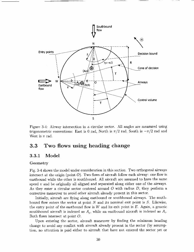
3-4 Airway intersection in a circular sector. All angles are measured using
trigonometric conventions: East is 0 rad, North is 7r/2 rad, South is
-7r/2 rad and West is 7r rad ........................ 30
3-5 Insert: simulation with constant inter-arrival spacing (5 nm). Main
plot: distribution of angular deviations .................. 32
3-6 Insert: snapshot of simulation with random inter-arrival spacing (uni-
form distribution over [5, 10] nm). Main plot: distribution of angular
deviations ................................. 32
3-7 Edges of the projected conflict zone for Ai and definition of X .... 35
3-8 Eastbound protection zone. Left: an aircraft Ai has already maneu-
vered. Right: by maneuvering appropriately, An uses Ai's conflict-free
solution ................................... 36
3-9 Plot of the eastbound flow protection zone for 6 = 0.05, where X "_
4.1 deg by Eq. (3.10)............................ 36
Plot of the eastbound protection zone overlaid with aj(O) and pj(O),
for 6 = 0.05 ................................. 37
Eastbound protection zone and the projected conflict zone of an air-
craft. Notes: loci shown here are not sketched to scale. "PCZ" stands
for protected conflict zone ......................... 38

3-12
3-13
3-143-15
3-16
3-17
3-18
3-19
3-20
3-21
3-22
3-23
4-1
Illustration of the proof. Top: If the hypothesis is true, then thereexists one southbound aircraft Aj that conflicts when Ai is fully to
the left. Left: However, this conflict southbound aircraft could have
not maneuvered and would still have found a conflict-free path be-
cause (Right) its projected conflict zone would have been inside the
eastbound protection zone where there are no aircraft, by hypothesis. 39
Divergence of 3 flows under decentralized, sequential resolution strat-
egy. The initial separation distance is 5 nm. Top: airspace simulation.
Bottom: amplitude of maneuver as a function of time of entry . . . . 42
A way to partition the airspace for three 120 deg oriented aircraft flows. 43
By performing a lateral displacement, an aircraft can be translated to
a safe spot (blank airspace). A buffer B can be added to account for
uncertainties and lack of maneuvering precision ............. 44
Uniformly changing aisle width does not help some aircraft to find a
"safe spot". Top left: h/Ds¢p = 1. Top right: h//Ds_p = 2. Bottom:
h/Ds_p --+ oc ................................ 45
A way to structure airspace for three 120 deg oriented aircraft flows, so
that the constraint on the flow that appeared in Fig. 3-16 is released.
This structure has been optimized to minimize the maximal lateral
displacement ................................ 46
Partition of the region of positioning for flow 2 with equilateral trian-
gles. Once such a partition has been identified, it is verified that any
aircraft along the original flight path axis is able to reach a protected
zone (dark triangles) via lateral displacement only ............ 47
Determination of safe optimal spots with a given structure. Non con-
flicting spots are blank. At each abscissa, the closest safe spot from
the original path is determined. The result is the solid line, exhibiting
periodicity. The maximal deviation is immediately derived ....... 48
Result of the systematic calculation of best safe spots under Matlab
for the structure shown in Fig. 3-17. Here, the unit u is 2D_p/v/3.
The results for flows 1 to 3 appear from top to bottom ......... 48
Top: Conflict resolution for 3 streams of 20 aircraft obtained by ap-
plying the structure shown in Fig. 3-17, maximum deviation is 32 nm.
Bottom: Conflict resolution for the same configuration via mixed inte-
ger linear programming, maximum deviation is 23.1 nm ........ 50
Illustration of our procedure-based, centralized control scheme for three
flows intersecting over the Durango VOR, Mexico. Chart imported
from Microsoft Flight Simulator ...................... 51
A procedure-based aircraft conflict avoidance system at Anchorage In-
ternational Airport (Alaska) ......................... 52
Layout of the New York Center Sector. All three major New York
airports are located in the shaded area. One sector has been singled
out to show how our model mimics the sectors with some realism. 57
10

4-2
4-3
4-4
4-5
4-8
4-9
4-10
4-11
4-12
4-13
Diagram of the system. Measured parameters are represented with
color markers consistent with those shown on plots. Top: Entry con-
trol. Bottom: Setup of the extended control law, which includes the
possibility to control a portion _ of the sector .............. 61
Path stretching: notations and corner point locus ........... 63
Deviation angle X (or XI) as a function of the apparent decrease in
(projected) speed Av/v = _, for a sector of length D = 150 nm and
width w -- 40 nm. The function is continuous and consists of two parts,
noticeable by the discontinuity of the slope at Av/v = _l _ -3.4%:
the left part is when symmetrical path stretching is used, and the right
part is when the upper limit on width (w) is reached and asymmetrical
path stretching is enforced ......................... 64
Snapshot of a sector under path stretching flow control. Sector length is
19 = 150 nm and width w -- 40 nm. Trajectories are shown in dimmed
lines. Top: Symmetrical path stretching. Bottom: Asymmetrical path
stretching .................................. 65
Simulation with deterministic scheduled arrivals. A restriction is im-
posed on the output rate at t = 1.5 hr .................. 68
Simulation with deterministic scheduled arrivals. A restriction is im-
posed on the output at t = 1.5 hr. Input control is active and lowers
the input rate at t_- 2.2 hr ......................... 69
Simulation with randomized arrivals. A restriction is imposed on the
output at t -- 1.5 hr ............................ 70
Simulation with 80_ of the sector controlled. A restriction is imposed
on the output at t = 1.5 hr ........................ 71
Simulation with deterministic scheduled arrivals. A restriction is im-
posed on the output at t = 1.5 hr and returns to 60 ac/hr at t = 2 hr. 72
Simulation with deterministic scheduled arrivals. A restriction is im-
posed on the output at t = 1.5 hr and returns to 96 ac/hr at t -- 2 hr. 73
Simulation with an enhanced aircraft model. The acceleration is lim-
ited to 0.4 kt/s. This plot should be compared with Fig. 4-9 as the
same simulation parameters are used: deterministic scheduled arrivals,
control over 80_ of the sector, restriction imposed on the output at
t = 1.5 hr and lifted ............................ 74
Geometrical approach to understand why capacity does not change
with the controlled proportion of a sector _. Shown in black and red,
solid lines are the time-space trajectories of aircraft either under single
entry control or control over _ of the sector ............... 76
11

12

Chapter 1
Introduction
1.1 Background
1.1.1 Current Air Traffic Control system
Current air transportation in the United States relies on a system born half a century
ago. While demand for air travel has kept increasing over the years, technologies at
the heart of the National Airspace System (NAS) have not been able to follow an
adequate evolution. For instance, computers used to centralize flight data in airspace
sectors run a software developed in 1972. Safety, as well as certification and portability
issues arise as major obstacles for the improvement of the system.
The NAS is a structure that has never been designed, but has rather evolved over
time. This has many drawbacks, mainly due to a lack of integration and engineering
leading to many inefficiencies and losses of performance. To improve the operations,
understanding of this complex needs to be built up to a certain level. This work
presents research done on Air Traffic Management (ATM) at the level of the en-route
sector.
1.1.2 Major issues
Today's air operations are characterized by an overwhelming emphasis on safety, with
little relatively attention paid to performance of the service provided by Air Traffic
Control (ATC) facilities. Although safety will always remain the most important task
to be performed by ATC, experts agree that some efficiency awareness is needed in
the system.
System-wide
The most obvious consequences of the NAS inefficiencies are the almost inevitable
delays experienced by commercial flights in the US. As the system handles an ever
increasing number of daily operations due to higher demand (see Fig. 1-1), it also
nears a capacity limit - although this number remains an unknown. The variation
in the last few years has shown that delays were increasing noticeably faster than
13

800O0
Annual number of enplanements in the United States
"or-
(n
0
E¢)
t.-UJ
700OO
60000
50000
40000
30000
200OO
10000
1950 1960 1970 1980 1990 2000
Years
Figure I-i: Number of enplanements over the last 50 years
2010
the number of daily operations. This high sensitivity is a sure indication of a system
approaching gridlock.
Summer 2000 delays During the summer of 2000, the delay problem became
widely publicized and public awareness was raised regarding the issues faced by the air
transportation community. Weather-related restrictions severely impacted the system
at that time and translated into dramatic delays. This amplification is a phenomenon
characterizing the lack of robustness attained when reaching the limit.
Fig. 1-2 shows the evolution of delays over the last few years. Since the terrorists
attacks of September llth, 2001, air traffic has globally decreased, and so did the
delays.
System sensitivity and delay back-propagation The state of congestion
attained by the NAS is illustrated by the following situation, which occurred in June
2000. On a clear weather day, a small demand/capacity imbalance at Newark Airport
(one of New York City's airports) propagated restrictions throughout the country in
15 minutes. Initially 5 aircraft in excess of the usual Newark landing capacity (45
aircraft per hour) led to 250 aircraft being held at airports or on holding patterns
throughout the country. Fig. 1-3 shows the evolution of the propagation in time.
Sector-wise
As the NAS is divided into smaller entities called sectors, the problems encountered
at the higher scale map to local areas. Human air traffic controllers are in charge
14

i
O"O
O
"Ot-
Or-.I-
60
50
40
30
20
,°I0 I I I I I I I I ] i
Jan Feb Mar Apr May Jun Jul Aug Sop Oct Nov
Month
r--2001
..... 2000
.... 1999
--1998
-.1997
---,1996
-.-1995
Dec
Figure 1-2: Monthly delay data over the last 7 years. A flight is delayed if it arrives
at destination more than 15 min later than its scheduled time of arrival.
ZDv
Figure 1-3: Propagation of a restriction in New York Air Route Traffic Control Center
throughout the country. (Source [391).
15

of managingaircraft in their sector, i.e. directing them from an entry point to anexit point while keepingeachairplane separatedfrom one another throughout theirflight. This separation is a minimum standard prescribedby the Federal AviationAdministration (FAA) in the US, which forbids en-route aircraft to get closerthan5 nautical miles (nm) from eachother at any time of their flight. En-route sectorsare sectorshandling aircraft at cruising altitude (usually above18,000ft). Terminalareasectors,alsocalledTRACONs, arecenteredon oneor moreairports, and controlaircraft up to a certain altitude.
Capacity limitations due to human controllers Because controllers are
human beings, they have a finite capacity to handle aircraft. Their main goal is to
guarantee safety, thus to maintain separation. Performance, and expeditious handling
of aircraft are only dealt with when time permits. Moreover, an upper limit on the
number of aircraft that can be handled simultaneously exists, although it is hard to
compute. References [18, 17] bring about the notion of complexity of a sector to
explain why this number varies with each particular situation.
Non-optimality of current control schemes The current concept of control
of air traffic relies on a fully centralized decision process. Control is performed at
the controller's level while aircraft are only the actuators. Such a centralized policy,
for all the safety it guarantees, does not perform well from an economic standpoint.
From the aircraft perspective, optimal parameters of flights (due to winds, aircraft
loading, optimal altitude or speed) are not always those actually flown.
1.1.3 Future improvements
Because of these system flaws, a lot of research and development work is currently
under way to improve the overall concept of operations. The certification process,
inherent to any safety-critical system, may delay for years the time when new concepts
will start being implemented nation-wide. A brief overview of these concepts follows.
Concepts
Free Flight Because of the centralized system inefficiencies mentioned above,
the ATM community focuses part of its work on the Free Flight concept. In this
scheme, every aircraft out of the terminal areas (departure and arrival sectors) is
solely responsible for maintaining separation with surrounding aircraft. The upside
of this constraint is the freedom gained by these aircraft to choose their flight path
independently. The assumption is that the aircraft decision makers - either the flight
deck, the airline operations center (AOC), or both - will optimize their flight path
according to their cost function.
This raises many questions about extreme situations. One critical scenario would
occur if a conflict encounter gets to a level of complexity beyond the capacities of any
implemented conflict resolution algorithm. The control would then be handed over
to stand-by human air traffic controllers, who then would be faced with an unusually
16

complexsituation. There is concernabout the accuracyand safety of the reaction ofthe human controllers.
The foundation of the concept itself might be discussedin terms of efficiency.Studieshavebeendoneto determineunder which assumptionsdecentralizedcontrolis moreefficient than the current, centralizedscheme(see[6,25]). A priori, this resultis not intuitive asthe greedinessof individual decisionsmay leadto an overall highernumber of conflicts that increasesthe time spent for conflict avoidanceon a typicalflight (due to the creation of a non-organizedflow by this scheme,contrary to thewell-structured flow of today's network of beaconsand airways- see[38]).
Distributed Air-Ground Traffic Management (DAG-TM) Building onthe idea of Free Flight, an entire concept of operation has been developed,whereair traffic control serviceproviders, airline operationscentersand flight deck inter-act (see[1, 24]). DAG-TM is an advancedATM conceptwhere decision processesare decentralizedand distributed among this triad of agents,which have differentresponsibilities.
Tools
Advances in the Air Traffic Managementconceptsheavily rely on new meansofcommunication,positioning and guidance.The following introducessomeof these.
Satellite Positioning System - Wide Area Augmentation System (WAAS)
Satellite Positioning technology lies at the heart of the envisioned air traffic system.
This technology has been popularized in the last decade with the American Global
Positioning System (GPS), as well as its Russian counterpart (Glonass) and the fu-
ture European system (Galileo). To gain in precision, the GPS has been augmented
with WAAS in the US. This, in conjunction with current ground facilities (radar,
navigation aids), is expected to deliver the level of accuracy and redundancy required
for the safe operations of aircraft.
Automatic Dependent Surveillance- Broadcast (ADS-B) To supplement
ground-based radar on the way to perform self-separation, one needs to know the po-
sitions of surrounding aircraft. This is achieved by broadcasting the position obtained
through the previously described system, and listening for neighbors' positions. This
system is in its demonstration phase and is expected to be first implemented in radar-
deprived areas, such as the Pacific Ocean, Siberia and polar regions. (see [2])
Center-TRACON Automation System (CTAS) A set of ATM tools has
been developed at NASA Ames Research Center under the name of CTAS. These
tools present real-time data to the controller in order for him to take appropriate and
optimal actions. As of today, they do not interact directly with the aircraft.
They currently mostly deal with the arrival and departure processes:
17

• A Terminal ManagementAdvisor (TMA), managing the arrival sequenceofaircraft;
• A DescentAdvisor (DA), generatingtimes of descentfor optimal sequencinginthe terminal area;
• A Final Approach SpacingTool (FAST), sequencingfinal approachpaths andrunway assignments;
• A SurfaceManagementSystem(SMS), for surfacemovementsmanagement.
Other tools exists, suchas the Direct-To (D2) tool that proposesen-route clear-ancesto be deliveredby the controller, taking separationsissuesinto account. Thisalonecan savepreciousminutes of flight and should be greatly appreciatedby theATC customers.
Someof thesetools werefield-testedat Dallas-FortWorth airport and encountereda great successon the controllers' side.
1.2 Motivation
Motivation for the present work arises from the ATM current state-of-the-art, and is
described next. It was conducted with the intention of gaining insight into modeled
scenarios of operations, on specific issues encountered by the system.
1.2.1 Worst-case scenarios
To deliver meaningful results of stability, worst-case scenarios were preferred to prob-
abilistic analyses. The number of daily operations (40,000 in the US alone) and the
certification requirements justify inquiring the more pessimistic scenarios.
For instance, if a flow of aircraft is supposed to carry aircraft separated at least
by the minimum separation distance Dsep, we will assume that they are separated by
exactly Dsep over an extended period of time. We also make sure that such hypotheses
do not overlook even worse cases. Stability results are derived from formal analysis
rather than from an extended number of simulations.
1.2.2 Separation
One part of this work concentrates on the problem of intersecting flows of aircraft.
Two or three flows intersect and each aircraft in each flow has to maintain separation
with all others. Centralized and decentralized processes of decision are analyzed and
stability proofs are given where available.
18

1.2.3 Scheduling and system overflow
A second part deals with the problem of input/output imbalance, and restriction
back-propagation, much in the way described in Section 1.1.2. An analysis of a sector
capacity is formally derived.
19

20

Chapter 2
Models
2.1 Aircraft
2.1.1 Kinematics
The mathematical approach of this work requires some simplifying assumptions. Air-
craft motion can be modeled in very different ways, and to very different levels of
realism. A purely kinematic model of the aircraft is used, ignoring the mass and
inertia parameters.
Consequently, an aircraft Ai is associated with a state-space vector (xl,vl), i.e.
position and speed. This fully characterizes the vehicle. With kinematics only, any
action on the speed vector vi is instantaneous. These actions, called maneuvers,
consist of turns or speed changes and happen immediately.
2.1.2 Maneuver library
Conflict avoidance maneuvers
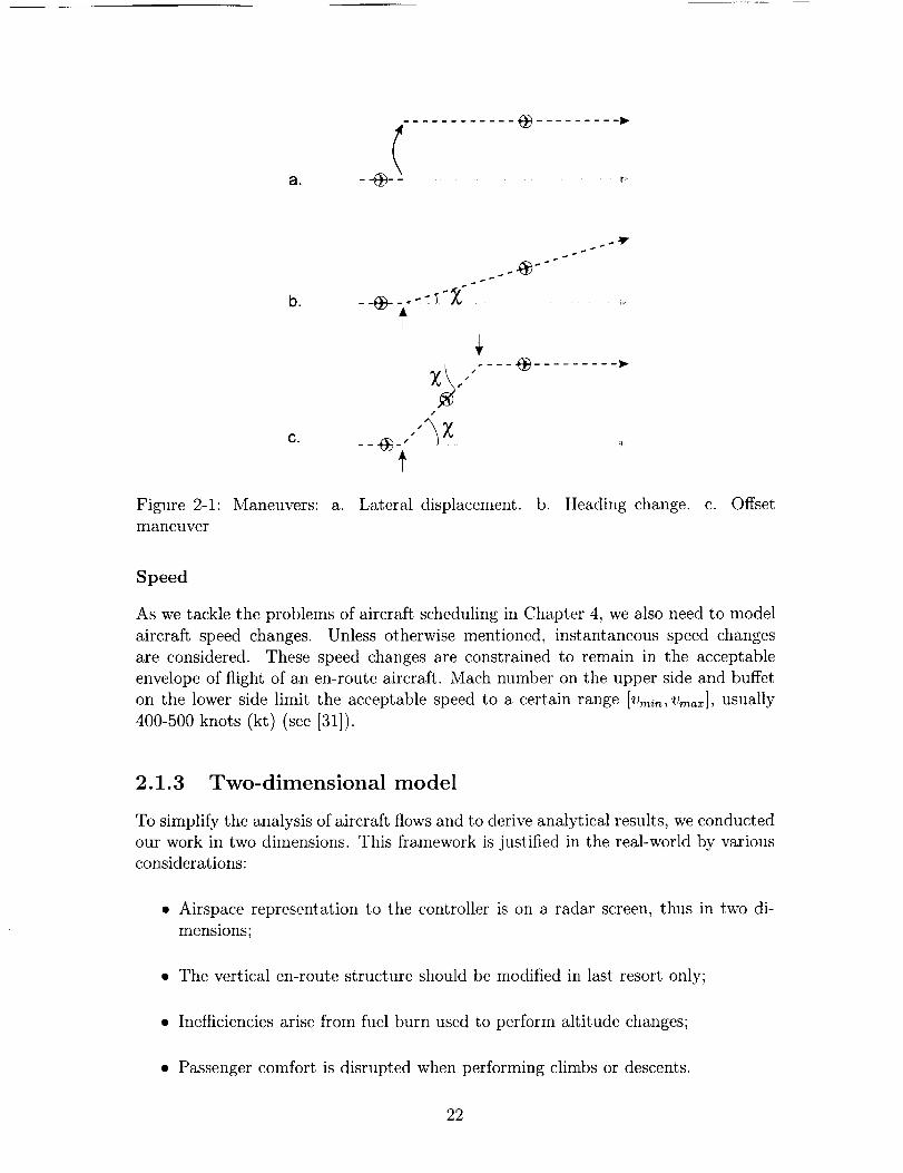
For conflict avoidance purposes, three models of maneuvers were used (see Fig. 2-1).
These models will be used mostly in Chapter 3.
• Lateral displacement: the controlled aircraft performs an instantaneous change
of position perpendicular to its route of flight. Its speed remains unchanged.
(Fig. 2-l-a)
• Heading change: the controlled aircraft changes heading instantaneously, mod-
ifying the direction of the speed vector. (Fig. 2-l-b)
• Offset maneuver: the controlled aircraft performs two successive heading changes,
while keeping its speed at a constant value. Both heading changes are of same
amplitude X, but opposite in direction. After the maneuver, the speed vector
returns to its original direction. (Fig. 2-1-c and [3])
21
a.
b.
Co
,s
Figure 2-1: Maneuvers: a. Lateral displacement, b. Heading change, c. Offset
maneuver
Speed
As we tackle the problems of aircraft scheduling in Chapter 4, we also need to model
aircraR speed changes. Unless otherwise mentioned, instantaneous speed changes
are considered. These speed changes are constrained to remain in the acceptable
envelope of flight of an en-route aircraft. Mach number on the upper side and buffet
on the lower side limit the acceptable speed to a certain range [Vmin, V,,_], usually
400-500 knots (kt) (see [31]).
2.1.3 Two-dimensional model
To simplify the analysis of aircraft flows and to derive analytical results, we conducted
our work in two dimensions. This framework is justified in the real-world by various
considerations:
• Airspace representation to the controller is on a radar screen, thus in two di-
mensions;
• The vertical en-route structure should be modified in last resort only;
• Inefficiencies arise from fuel burn used to perform altitude changes;
• Passenger comfort is disrupted when performing climbs or descents.
22

2.1.4 Safety distance
To account for the FAA separation distance of Dsep = 5 nm, a 2.5 nm-radius safety
zone is attached to each aircraft. The 5 nm separation standard is thus violated if
two of these circular zones intersect.
Although a vertical separation limit of 2000 ft (1000 R under the new Reduced
Vertical Spacing Minimum program) exists in the real world, it is not be taken into
account here because of the two-dimensional model explained above.
2.2 Sector and aircraft arrival
In both Chapters 3 and 4, aircraft need to meet a certain kind of requirement at a
given point. In Chapter 3, this requirement consists in maintaining separation at the
intersection of two or three aircraft flows. In Chapter 4, a scheduling constraint exists
at the exit of a sector.
This translates into zones of control of a certain length D. In the case of aircraft
flows intersection, we thus have a circular sector of radius D, whose center is the
intersection (see also [9]). In the scheduling case, we have a rectangular sector, of
length D, and width w: the scheduling constraint has to be met at a distance D from
the entry fix.
Aircraft enter the sector at prescribed entry points, mimicking the network of
fixes existing in the real world. The only assumption on their arrival is a guarantee
that inter-arrival spacing is at least Dsep: this is a reasonable assumption stating that
aircraft are not in conflict when entering.
2.3 Control schemes
Control is applied to aircraft in flows, whether centralized or decentralized. Except
when otherwise mentioned, an aircraft receives only one instruction through its entire
flight in the sector. Depending on the situation, this one instruction is either a
maneuver or a change in speed, as described in Section 2.1.2.
2.3.1 Decentralized
A decentralized control scheme is applied when possible. Each aircraft makes its
own, greedy maneuver to perform adequate separation or scheduling requirement.
This models the Free Flight distributed concept of operations.
2.3.2 Centralized
A centralized control scheme is used in Section 3.4. This is an exact parallel with
what is done today in the ATC system, where the controller performs centralized
control.
23

2.3.3 First In- First Out policy
A First-In First-Out policy is implemented in all of our models. Aircraft leave the
sector in the order they entered, i.e. no overtaking is allowed. This policy is widely
recognized as the fairest.
2.4 Metrics
Precise stability and metrics description are further explained in Chapters 3 and 4.
Following is only a quick overview of the ideas.
2.4.1 Stability
We characterize stability of aircraft flows under constraints as the state in which no
conflict occurs at any time using acceptable maneuvers of bounded amplitude.
2.4.2 Capacity
Capacity is a number of aircraft that can be processed by a sector for a particular
task (e.g., delaying aircraft).
24
Chapter 3
Control of intersecting flows under
separation constraints
3.1 Background
Conflict Detection and Resolution (CD&R) has attracted considerable attention over
the last decade. A 2000 survey [26] related the existence of 68 different CD&R
modeling methods.
The research community addressed problems related to Air Traffic Management in
a great variety of approaches. In line with today's concept of operations, centralized
control approaches are used to provide globally optimal control of pools of aircraft
operating in the same airspace. Different mathematical formulations are taken, such
as semi-definite programming [15], mixed integer programming [37], optimal control
[19], genetic algorithms [16], or a combination of the above [32]. These approaches
provide optimal path planning for a finite number of aircraft performing online com-
putations. Some innovative approaches make use of other fields of research: hybrid
systems [4], optical networks theory [33], or self-organized criticality [27].
Decentralized control is also addressed in a number of papers to provide theoretical
background to the future Free-Flight concept (see Section 1.1.3). Once again, different
approaches are taken, such as: mixed integer linear programming [36], analytical
geometry [5, 28, 29, 30], or hybrid systems [20]. Procedure-based control appears in
a few papers such as [8, 20].
The present work concentrates on an infinite number of aircraft involved in po-
tential conflicts. Aircraft are organized along airways in infinite flows that intersect.
Potential conflicts occur at the intersection and aircraft maneuver independently to
avoid violating safety distances. One originality of this work lies in the proof of sta-
bility (i.e. safety) of the control law over any amount of time and with any numberof aircraft in each flows.
Section 3.2 shows the stability of two intersecting flows when aircraft use the offset
maneuver to perform conflict avoidance. Section 3.3 presents the same result for air-
craft using heading changes, although the proof is more involved than in Section 3.2.
Section 3.4 addresses the problem of three intersecting flows. Because the decentral-
25

ized control usedin the two precedingsectionsdoesnot yield stability in that case,centralizedcontrol is usedto createa procedure-based,stable scheme.
This chapter presents results that appeared in [11] and [12]. Appendix A gives a
summary of simulations appearing in this thesis.
3.2 Two flows using offset maneuver
The problem of two intersecting flows of aircraft that must maintain separation is
addressed in this section. Considering the offset maneuver for conflict avoidance (see
Section 2.1.2), simulations are performed and a stability analysis is provided.
3.2.1 Model
The following model of operations is considered: two flows of aircraft intersect at the
center O of a sector of radius D, called control volume. Each flow enters through a
fix, either W (West) or N (North), with the intention of leaving the sector through
E (East) and S (South) respectively. All aircraft fly at constant and uniform speed.
Each aircraR can observe the state of all aircraft already inside the control volume
(using an idealization of ADS-B, for instance). Each aircraft can take a single ma-
neuver at the instant it enters the control volume. This maneuver must have minimal
amplitude and must be conflict-free; this assumption models a real-world system in
which pilots make safe, lowest-cost, decentralized decisions.
Offset maneuver and lateral displacement The offset maneuver is shown
in Fig. 2-1-c and with more details in Fig. 3-1. It consists of two successive heading
changes of fixed amplitude iX. This type of maneuver is considered realistic and
air traffic controllers use it to handle conflicts. The amplitude of the maneuver is
modulated by the length of "inclined" leg.
Comparing with the lateral displacement model (see Fig. 2-l-a), the offset ma-
neuver considered in this section is equivalent to a lateral jump of size d and a lon-
gitudinal, backward jump of size dtan (X/2) (see Fig. 3-1). This important remark
simplifies the stability analysis by making the proofs presented in [29] almost directly
applicable to the current model. One difficulty arises here as the inclined leg is not
included in the conflict resolution analysis, and must still be conflict-free. Therefore,
we assume the offset maneuver area is sufficiently far from the conflict itself. Under
these conditions, the maneuver reduces to choosing a position, when entering the
control volume, along a line inclined at an angle of value +(_r/2 + X/2) with respect
to the direction of flow. This angle is positive if the deviation occurs to the left and
negative to the right.
We wish to derive the largest lateral deviation necessary for conflict resolution.
As in the analysis presented in [29], we define a corridor of width dmax, within which
each aircraft can maneuver (Fig. 3-3). It is shown that for dr_ax large enough, there
always exists a maneuver within that corridor such that any conflict can be solved.
26

inclined leg
d tan X/2 second ATC control
!'i'i\.....................,/_Y _ Td; i
first ATC control
Figure 3-1: Offset maneuver
3.2.2 Simulations
Fig. 3-2 shows the result of a simulation using 250 aircraft in both flows, with an
initial separation subject to a uniform distribution on the interval [5, 15] nm. A
plot of the population of deviations is given along with a snapshot of the control
volume at one instant during the simulation. Data from a set of 20 simulations are
available, although only one instance is represented here. This data show a recurring
characteristic appearing in the deviation distribution: no aircraft ever deviated more
than _ 7.5 nm. Equivalently, all aircraft found conflict-free path by performing an
offset maneuver that took them no further than 7.5 nm away from their original
planned trajectory.
This result, as well as the overall geometry of the control volume, should be
paralleled with that of Mao et al. (see [28, 29, 30]).
3.2.3 Stability proof
Existence of a bounded conflict resolution offset maneuver draws from the analy-
sis found in [29]. Parameters of interest are the separation distance Ds_; and the
encounter angle (90 deg, in this case).
Consider an aircraft entering the control volume. Assume without loss of gener-
ality that this aircraft is eastbound and denote it A_, as in Fig. 3-3. We show that
this aircraft can always execute a bounded offset maneuver of amplitude less than or
equal to dm_, if dm_ = v/2D,_v, which results in a conflict-free trajectory.
We prove this fact by contradiction, assuming in the first place that such a ma-
neuver does not exist.
Hypothesis: Ai cannot find a conflict-free maneuver of amplitude smaller than dm_x
Each aircraft within the control volume projects an "aisle" (oriented at a 45 degree
angle in the case of orthogonal aircraft flows), such that no aircraft from the opposite
flow can enter this aisle without creating a conflict.
The aisles created by the eastbound aircraft ahead of Ai should not cover the
protected circle of A_, wherever Ai is located within its maneuver corridor. Indeed, if
the converse were true, Ai could hide behind the aircraft by moving sideways and thus
find a conflict-free trajectory with an offset maneuver of amplitude d less than dma=
27

f-v
150
100
50
-50
-100
oo@8®N
W / __ E_®_ .,_ _ ® _ ® ® ®,,, _® I® .®
®S®
-150 , , z , , J-150 -100 -50 0 50 100 150
x (nm)45
40
35
C 30
0 1 2 3 4 5 6 7
Absolute value of lateral displacement (nm)
Figure 3-2: Simulation for random arrival using offset maneuvers. Original separation
is uniformly distributed on [5, 15] nm. 250 aircraft are simulated in each flow. Top:
Snapshot of the simulation. Bottom: Aircraft deviation distribution.
28

I
dmax
i
' Edmax
I
I
S
Figure 3-3: Existence of conflict resolution maneuver with the offset maneuver.
which is contradictory with the above assumption. Stated differently, there should
be no aircraft other than Ai within the shaded area P (shaped like a skewed arrow
tip) in Fig. 3-3.
Meanwhile, all southbound aircraft already inside the control volume have already
performed their own maneuver leading to conflict-free trajectories, and are flying
along straight southbound paths. Under the above hypothesis, their aisles intersect
the protected circle of Ai for all possible offset maneuvers of Ai within the corridor.
In particular, this is true when Ai performs a left offset maneuver of amplitude dma_,
as shown in Fig. 3-3. Therefore, a southbound aircraft Aj (shown on the figure) is
in conflict with Ai and must have deviated to the right by an amplitude d such that
d > dmax - Ds_pV/-2 = O.
However, because the area P is empty of any eastbound aircraft, the aircraft Aj
would have been safe by maneuvering to the right by an amplitude strictly less than d.
This implies that Aj's maneuver did not have minimum amplitude. It also contradicts
the requirement that the maneuver of each aircraft must have minimum amplitude.
Thus the amplitude of the aircraft deviation is bounded and its maximum value is:
dma_ : v/-2Dsep. (3.1)
This result applies to Figure 3-2 where v_Ds_p = 7.1 nm, and explains the limit
found in the heading distribution plot.
29
Entry points
_ Southbound
flow
N
Decision bound
R
decision
Eastbound
flow
TControl volume
Figure 3-4: Airway intersection in a circular sector. All angles are measured using
trigonometric conventions: East is 0 rad, North is _r/2 rad, South is -7r/2 rad and
West is 7r rad.
3.3 Two flows using heading change
3.3.1 Model
Geometry
Fig. 3-4 shows the model under consideration in this section. Two orthogonal airways
intersect at the origin (point O). Two flows of aircraft follow each airway: one flow iseastbound while the other is southbound. All aircraft are assumed to have the same
speed v and be originally all aligned and separated along either one of the airways.
As they enter a circular sector centered around O with radius D, they perform a
corrective maneuver to avoid other aircraft already present in this sector.
Initially, aircraft are flying along eastbound or southbound airways. The south-
bound flow enters the sector at point N and its nominal exit point is S. Likewise,
the entry point of the eastbound flow is W and its exit point is E. Again, a generic
southbound aircraft is indexed as A j, while an eastbound aircraft is indexed as Ai.
Both flows intersect at point O.
Upon entering the sector, aircraft maneuver by finding the minimum heading
change to avoid any conflict with aircraft already present in the sector (by assump-
tion, no attention is paid either to aircraft that have not entered the sector yet or
30

have already left). This is the only maneuveraircraft can perform; after maneuver-ing, aircraft movealongstraight linesasdefinedby their original (and only) headingchange.This conflict resolution schemeimplementsthe First-Come First-Servedpri-ority stated in Section 2.3.3. A conflict is declared if the minimum miss distancebetweentwo aircraft is lessthan Dsep.
Coordinate system
In addition to the usual cartesian coordinate system (origin O, x pointing to the East,
y pointing to the North), two systems of polar coordinates are used for southbound
and eastbound aircraft, as shown in Fig. 3-4. The position of a southbound aircraft
Aj in the sector is given by the polar coordinates (a,r/), where a is the distance
between N and the aircraft, and r/ is the directed angle between the vector NAj and
the eastbound direction. Likewise the position of eastbound aircraft is noted (b, 0).
Scaled variables
The radius of the sector is the reference length. The following non-dimensional vari-
ables are defined:
(_ D_p a b=- /3 (3.2)D' D' =D'
as well as the scaled speed:V
D
3.3.2 Simulations
Simulations of the above system have been performed in Matlab. The radius D of
the sector radius is assumed to be 100 nm. The speed of each aircraft is 400 kt, and
Ds_p is assumed to be 5 nm (thus _ = 0.05). Aircraft enter the sector at regular orrandom time intervals.
Two illustrative simulations are shown in Figs. 3-5 and 3-6. Fig. 3-5 shows a
simulation involving aircraft entering at regular time intervals with 250 aircraft in
each flow. The aircraft are entering the sector spaced exactly by 5 nm. As might be
expected, the resulting pattern obtained by simulation is periodic and bounded.
Fig. 3-6 shows the conflict resolution process resulting from a random aircraft
arrival process: the spacings between two consecutive aircraft in the southbound or
eastbound flows are uniformly distributed over the interval [5, 10] nm. The simulation
involved 250 aircraft in each flow. The population of heading change commands shown
on the distribution plot remains bounded.
3.3.3 Stability proof
Motivated by these simulations, we now proceed with a proof that heading changes
generated by conflict avoidance maneuvers remain bounded. Without loss of general-
ity, the notion of projected conflict zone for an eastbound aircraft is first introduced,
31

0.7
0.6
0.5
0.4
o
a. 0.3
0.2
0.1
_0
0000
0 o
©0
©©
©©©
0 I I1 0 1 2 3 4 5 6 7
Angle of deviation in degrees
Figure 3-5: Insert: simulation with constant inter-arrival spacing (5 nm). Main plot:
distribution of angular deviations.
0.35 r
0.3
0.25
0.1
0.05
00
=0.2o
o=a0.15
0
8
00
%0
0
_o_oCb_ooooO_oOoOoO oo o o°'J""O 0 0 0
00
00
oo©
0©
©
0 0
1 2 3 4 5 6
Angle of deviation (deg)
Figure 3-6: Insert: snapshot of simulation with random inter-arrival spacing (uniform
distribution over [5, 10] nm). Main plot: distribution of angular deviations.
32

followed by that of eastbound protection zone for an eastbound aircraft Ai. Armed
with these notions, we conclude with a proof that aircraft angular deviations remain
bounded.
Projected conflict zone of an eastbound aircraft
For a given aircraft Ai that has already maneuvered, consider the locus of the south-
bound aircraft positions resulting in a conflict with Ai. This locus is called projected
conflict zone and is sketched in Fig. 3-7. It is this case equivalent with the "aisles" of
the offset maneuver case (Section 3.2). It is worth noting that this locus is quite com-
plex in shape and changes with the aircraft heading and its position. If the projected
conflict zone intersects with any southbound aircraft, the corresponding heading for
aircraft Ai is not conflict-free. An analytic expression for the projected conflict zone
is now derived.
The starting point is the locus (c_, rl) of southbound aircraft Aj that would get
into conflict with A_. We first derive their positions and velocities as functions of ct,
and ,, whose definitions are given by Eq. (3.2) and Eq. (3.3).
The positions of the aircraft Ai and potential intruder Aj are written in normalized
cartesian coordinates:
( cos0) (ocos )WAI = fi sin 0 , NAj = a sin r/ '
Likewise the scaled velocities of these aircraft are expressed:
vA, = _ sin 0 , vAj = v sin r/ "
Ref.[23] derives expressions for the normalized relative speed c = (c,_, %)T:
c = VAj -- VA, (3.4)
the relative position vector r = (r_, ry)T:
( -c_cosrl +t3cos0- 1 )r:-c_ sinr] + _3sin0- 1 '
(3.5)
and the minimum approach distance m:
m=c×(r×c). (3.6)
The above formulae lead to the minimum approach distance for Ai and Aj"
m 2 rxcy -- ryCx) 2
((-0_% + rico - 1)(s0 - s,7) + (as, - flso + 1)(c0 -%))2
2 - 2%co - 2s,Tso
33

where sin0 and cos0 have been replaced by the shorthands so and Co, and likewise
for r/.
We now derive an expression to describe the boundary of the projected conflict
zone for an incoming eastbound aircraft Ai. Rather than plotting this projected
conflict zone when A_ enters the sector, we plot it when Ai has traveled the normalized
distance 1/2 in the sector (i.e. R/2 in the dimensional space), thereby considerably
simplifying its graphical representation. We derive the a(r/) that yield a minimum
approach distance rn of exactly the minimum separation distance (_: the desired zone
is obtained by solving the equation m 2 = 5 2 in the variable ct. The two roots of this
equation, which are the locus as a function of c_(r/), are:
1 (sos, 7 + so% + cos o -coc, 7 + 1) - 5v/-2v/1 + soSo - co% (3.7)p(rl) - 2 so + s_ '
1 (SOS,7 + So% + CoS, - CoC,1 + 1) + 5V_v/1 + SoS, 7 - CoC_ (3.8)_r(_) - 2 so + s_
These define the projected conflict zone of Ai(_, 0) in the southbound flow's co-
ordinate system (see Fig. 3-7 left).
Note: the aisle has a different meaning in Section 3.2 than the projected conflict
zone has here. The aisle of an eastbound aircraft in Fig. 3-3 must not intersect the
safety zone of a southbound aircraft (see Section 2.1.4). Here, the projected conflict
zone of an eastbound aircraft must not include the position of a southbound aircraft.
Intersection of the projected conflict zone of an eastbound aircraft with
the set of heading angles available to a southbound aircraft
We call decision bound the two arcs centered at W or N, of radius 1/2 and spanning
the angular range [-X, X]. Let T be the maximum heading change allowed for aircraft
of each flow. Equivalently: eastbound aircraft maneuver in [-T, T] and southbound
aircraft in [-7r/2 - T,-7r/2 + T]. Consider the angular range width X, defined as
the unusable heading range for a southbound aircraft on the southbound decision
bound (a = 1/2) due to the presence of an aircraft on the eastbound decision bound
(/3 = 1/2, 0 = T). Fig. 3-7 illustrates this configuration.
Defining r/* such that a(rfl) = 1/2, X is expressed as:
7rX = T + rfl + -. (3.9)
2
Geometric considerations show that:
tan X --5v_- 55
1 - 5 2(3.1o)
34

N
_W ............
Figure 3-7: Edges of the projected conflict zone for Ai and definition of X
Eastbound flow protection zone
We now introduce the notion of protection zone, which is the equivalent of the area P
in Fig. 3-3 of Section 3.2.3. Consider the case whereby an eastbound aircraft Ai+l is
about to enter the sector. Assume moreover that it is preceded by another eastbound
aircraft Ai, which has already maneuvered so as to find a conflict-free trajectory. By
definition, the projected conflict zone of Ai does not contain any southbound aircraft.
Can Ai+l take advantage of the fact that Ai is on a conflict-free trajectory to gen-
erate its own conflict-free trajectory? This would be the case if Ai+l could maneuver
so as to include its own projected conflict zone within that of Ai, as shown in Fig. 3-8.
It turns out there is a considerable range of positions of A_ for which the projected
conflict zone of A_+I is included in the projected conflict zone of A_ for a suitable
heading change 0n of Ai+l.
We define the eastbound protection zone as the locus of possible positions of Ai
satisfying the following conditions: (i) the heading of A_ is within the range I-X, X];
(ii) there exists a heading change 0n for which the projected conflict zone of Ai contains
that of Ai+l.
The numerically computed figure of this protection zone for 5 = 0.05 is shown in
Fig. 3-9.
An analytic computation of the eastbound protection zone for any value of (_ would
be preferable. It should be the object of future research efforts. The mathematical
problem of interest for the proof appears in Appendix B.
35

N N
.-" zon .. ..
Ne ")" air,teflon.providing
Figure 3-8: Eastbound protection zone. Left: an aircraft Ai has already maneuvered.
Right: by maneuvering appropriately, An uses Ai's conflict-free solution.
-X 4
3
2
1
_5-.1
-2
-3
-Z40 2 4 6 8 10 12 14 16
b (nm)
Figure 3-9: Plot of the eastbound flow protection zone for _ = 0.05, where X -_ 4.1 deg
by Eq. (3.10).
36

2 4 6 8 10 12 14 16
b (nm)
Figure 3-10: Plot of the eastbound protection zone overlaid with aj(O) and pj(O), for5 = 0.05.
Intersection of the projected conflict zone of a southbound aircraft with
the eastbound protection zone
A southbound aircraft Aj choosing a heading _ = -_/2 satisfies the following prop-
erty: its projected conflict zone is completely contained in the eastbound protection
zone.
Combining the numerical data from Section 3.3.3 with the expressions aj(0) and
&(0) (the subscript j is added to make clear these functions concern the southbound
flow) for the edges of the projected conflict zone of Aj, we numerically validated the
above property for any (_ < 0.2 (see B). A result is shown for 5 = 0.05 in Fig. 3-10.
Proof and bound
Armed with these results, we can now complete the stability analysis for two inter-
secting flows of aircraft, when the aircraft perform heading change maneuvers. The
following is an argument that stands very close to that used in Section 3.2.3. It is
shown that an aircraft entering the sector, say the eastbound aircraft Ai, can always
perform a heading change maneuver that results in a conflict-free trajectory, and this
maneuver is bounded above.
We make the following hypothesis, and show a contradiction:
Hypothesis: There exists an aircraft Ai for which no conflict-free path can be found
in the angular interval [-T, T] around its original heading, with T > X, and
ave- atanx - 1 - 52
37

N
PCZofAi/ \ / \
Eastgo.una 4,
o;o /New'comer _ ")" Pi:c:a_tion.providing
Figure 3-11: Eastbound protection zone and the projected conflict zone of an aircraft.
Notes: loci shown here are not sketched to scale. "PCZ" stands for protected conflict
zone.
If there were eastbound aircraft within the eastbound protection zone in front
of A_, their presence would provide a conflict-free path for Ai (by definition of the
eastbound protection zone, see Section 3.3.3): by taking an appropriate heading, Ai
would be able to move its projected conflict zone completely inside the projected
conflict zone of an aircraft ahead, thus getting a conflict-free path solution. Fig. 3-11
shows a sketch of the location of these aircraft able to provide "help" to newcomers.
Thus, there cannot be such aircraft within the eastbound protection zone because of
the hypothesis.
At the same time, all southbound aircraft currently inside the sector have already
performed their minimum heading change maneuver, and are flying along straight,
conflict-free southbound paths. Our hypothesis implies that there exists a southbound
aircraft on a conflict path with Ai for any heading change of Ai within the interval
[-7, T]. In particular, when A_ deviates fully to the left (i.e. 0 = +T), it remains
in conflict with at least one southbound aircraft Aj. This also implies that Aj must
have deviated by T-X > 0 (X does not depend on T, as shown above) to the left (i.e.
its new heading is less than -7r/2 - T + X) so that it is inside the projected conflict
zone of Ai.
However, if Aj had not deviated (r/= -7r/2), it would have found a conflict-free
path because its projected conflict zone is then free of conflict: it was shown above
that its projected conflict zone is completely contained in the eastbound protection
38

N
N N
%wPrzone
Figure 3-12: Illustration of the proof. Top: If the hypothesis is true, then there exists
one southbound aircraft Aj that conflicts when As is fully to the left. Left: However,this conflict southbound aircraft could have not maneuvered and would still have
found a conflict-free path because (Right) its projected conflict zone would have been
inside the eastbound protection zone where there are no aircraft, by hypothesis.
39

zone, which is itself free of aircraft (see Fig. 3-12).
Therefore, there is a contradiction with the initial hypothesis, and the following
is true: there always exists a solution (conflict-free path with heading change) within
the interval [-X,X], for all aircraft. By symmetry, the statement is true for both
flOWS.
The next paragraph shows a simple construction where the deviation is exactly X
and X is thus a tight bound on the maximum deviation.
We recall the expression Eq. (3.10) found above for X:
tan X --1 - (f2
It is interesting to notice that Eq. (3.10) can be linearized for small _ resulting
in )/ = _v_, yielding the result of Section 3.2.3 and [30] for the maximum lateral
displacement in the area of conflict: dmax = Dsepv_.
One-on-one conflict
There exists a configuration where tile heading change equals the value found in Eq. (3.10).
This configuration is a one-on-one confrontation. Two aircraft, one from each flow,
arrive in the sector at the same time. We can assume without loss of generality
that the southbound aircraft maneuvers first. The angle of deviation needed for the
eastbound aircraft to avoid the southbound one is :g.
3.4 Three flows using lateral displacement
This section considers the case of three intersecting flows of aircraft. The motiva-
tion for this extension is to build some understanding about the structure of inter-
secting flows of aircraft when coming from many different directions. Sequential,
decentralized control laws do not generate stable closed-loop flow behaviors. A cen-
tralized, procedure-based, optimized control policy is proposed: spatial structuring
of the airspace is identified that allows to support such an approach.
3.4.1 Model
To simplify the analysis, this section returns to the aircraft maneuvering model of
lateral displacement originally considered in [29] and described in Section 2.1.2 (see
Fig. 2-l-a). Such a model is justified in the case where the conflict area is well located
in time and space. A heading change AX is then modeled as an instantaneous lateral
jump of amplitude DAx where D is the "distance to conflict". Similarly, a velocity
change Av could be modeled as an instantaneous longitudinal jump of amplitude
AvD/v where v is the nominal velocity of the aircraft.
The conflict geometry under study is that of three aircraft flows converging to a
single point. The flows are symmetrically oriented with respect to the origin. Aircraft
in each flow are assumed to follow the same initial trajectory and then enter a circular
40

control volume. Again, to avoid in-trail conflicts, the inter-aircraft spacing is no lessthan Dsep.
3.4.2 Simulations
Fig. 3-13 shows that a sequential conflict resolution scheme may lead to unstable flow
behavior: three aircraft streams avoid conflicts arising due to interaction with the
other flows, using lateral displacements in the way described in Section 3.2. Aircraft
are allowed to perform only one conflict resolution maneuver when they enter the con-
trol volume, and consider other aircraft already within the control volume as moving
obstacles they must avoid. Fig. 3-13 shows that the lateral deviations experienced
by each flow become very large under such a control scheme. Further simulations
(not shown in this figure) indicate aircraft deviations keep diverging. Therefore, a
decentralized scheme is not appropriate for three flows.
3.4.3 Stabilization by centralized control
Many centralized approaches exist to solve conflicts that may not be solved via sequen-
tial approaches, including via on-line numerical optimization [29, 30, 35]. However,
these approaches are not necessarily guaranteed to converge to an optimal or even
feasible solution (indeed, the resulting optimization problems are often very com-
plex). This creates a significant problem when system safety is involved such as in
air transportation. We now show that centralized, optimization-based conflict reso-
lution strategies are stabilizing for three intersecting flows by providing an explicit,
feasible and bounded solution to that problem. While the procedure is described on
three symmetrically arranged aircraft flows, we believe it can be extended to other
encounter angles as well.
Meshing the space with projected conflict zones
The idea builds from Fig. 3-14. Aircraft from each flow project two "shadows" of
width Dsep aligned along their relative velocity vector with respect to the other two
aircraft flows. As described in Section 3.2, no aircraft from the other flows may be
within these shadows without creating a conflict. The aircraft arrangement shown in
Fig. 3-14 is able to cope with densely packed aircraft flows (where aircraft initially fol-
low each other at minimum separation distance in each flow), while avoiding conflicts
and generating only bounded aircraft deviations. Moreover this partition is valid for
an arbitrary large number of aircraft. However, this flow resolution structure requires
significant velocity control. A more desirable solution would try and avoid velocity
control, and concentrate on offset maneuvers instead.
Fig. 3-14 may however be used as an inspiration to construct an airspace parti-
tion that may handle infinite intersecting flows via lateral deviations only. The idea
is to generate an airspace partition using appropriately constructed aisles (aligned
along relative velocity vectors) and resulting spots where aircraft in each flow may
41

E¢-
v
2O0
15O
100
5O
-50
- 100
-15O
Flow
-200 ' _ _ _ ' ' ' '-200 -150 -100 - 50 0 50 100 150 200
x (nm)
Deviation histograms100
I I I I I I
% 5 10 15 20 25 30 35
v150 /
F°I Flow 2
o ; t'o ,'5 2'o ;5 _o 35100 , , , , ,
50
Flow 3
°o 5 ,o ,5 2'o 25 3'oAircraft #
35
Figure 3-13: Divergence of 3 flows under decentralized, sequential resolution strategy.
The initial separation distance is 5 nm. Top: airspace simulation. Bottom: amplitude
of maneuver as a function of time of entry
42

AI Flow 1
I
I
I
I
Allowed spots :
Flow 1 _ Flow 2 Flow 3
Figure 3-14: A way to partition the airspace for three 120 deg oriented aircraft flows.
43

Figure 3-15: By performing a lateral displacement, an aircraft can be translated to a
safe spot (blank airspace). A buffer B can be added to account for uncertainties and
lack of maneuvering precision.
locate themselves to avoid aircraft in the other flows (Fig. 3-15). Such a concept was
proposed in a different context in [21].
Robustness to arrival process
One available design variable when constructing this structure is the width of each
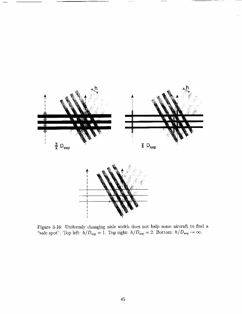
aisle. However, as shown in Fig. 3-16, choosing the same aisle width for each flow
does not result in any improvements, because for some initial aircraft locations along
their nominal path, there exist no lateral deviation leading to a safe "spot" via lateral
deviations only (these locations are shown with black lines on the figure).
Feasible solutions are obtained if the airspace is structured with different aisle
width patterns for each of the three aircraft flow pairs. The structure shown in
Fig. 3-17 can handle any aircraft flow as described at the beginning of this section;
as such it provides a bounded, feasible initial flow configuration that may be used for
example as a starting point for an on-line optimization procedure. This solution has
been optimized to minimize the maximal lateral displacement using a randomized
search algorithm. It is then compared with solutions obtained with mathematical
programming software for finite sets of aircraft belonging to three flows.
For the three flows, we outlined the spots where aircraft could be positioned. As
noted, the size of each aisle to safety distance ratio (h/Dscp) is now different for each
flow pair interaction, and the pattern of aisle, periodic. As can be inferred from the
way our structure has been constructed, the region where the positioning occurs can
be partitioned with equilateral triangles whose edge length is 4Dscp/v'_, as shown
for flow 1 in Fig. 3-18. This airspace decomposition allows aircraft from any flows to
perform lateral maneuvers and find a conflict-free location, as proven thereafter.
44
_Dsep Dsep
A
!:!!
I
Figure 3-16: Uniformly changing aisle width does not help some aircraft to find a
"safe spot". Top left: h/Dsep = 1. Top right: h/Dsep = 2. Bottom: h/Ds_p _ oo.
45

Flow 3f
oS
\
AI
I
I
I
I
I
ii
Flow 1
: !!
_o
Flow 2
Allowed spots :
Flow 1
Flow 2
Flow 3
Note • the safety circlehas been resized
Figure 3-17: A way to structure airspace for three 120 deg oriented aircraft flows, so
that the constraint on the flow that appeared in Fig. 3-16 is released. This structure
has been optimized to minimize the maximal lateral displacement.
46

Figure 3-18:Partition of the regionof positioning for flow 2with equilateral triangles.Oncesuch a partition has beenidentified, it is verified that any aircraft along theoriginal flight path axis is able to reacha protected zone (dark triangles) via lateral
displacement only.
Optimization of the geometry and performance bound
Consider Fig. 3-19. We represent the allowed spots as a function of the abscissa for
flow 1 with the aisle structure in the background. Other spot locations may also be
feasible, as sometimes a displacement to one side of the original track is equivalent
in cost (distance from the axis) to a displacement to the other side. The plot is
periodic, due to the periodicity of the crossing patterns. For flow 1 (Fig. 3-19), a
whole period is shown, which corresponds to a length of 24D_p. The spot locations
are systematically computed by Matlab for the three flows and are shown in Fig. 3-20.
It is noted that the period for flow 2 is 40Dsep, and for flow 3, 60D_p. By inspection
of Fig. 3-20, the maximum deviation experienced occurs in flows 2 and 3, for a value
of:
dmax = 6.4Ds_p. (3.11)
This gives a maximal overall lateral displacement of 32.0 nm as well as an upper
bound on the maximum lateral deviation that may be performed by aircraft. This is
far from being a realistic value and cannot possibly be applied "as is" for practical
flow management purposes. However, it may be of value to get some understanding
of the way conflict resolution processes work.
Comparison with mixed integer programming optimization
The conservatism of the solution proposed in the previous section may be evaluated
using numerical optimization procedures on particular, finite aircraft flow instances.
47

Max.deviation
tE 1 period !
Figure 3-19: Determination of safe optimal spots with a given structure. Non con-
flicting spots are blank. At each abscissa, the closest safe spot from the original
path is determined. The result is the solid line, exhibiting periodicity. The maximal
deviation is immediately derived.
5
0
-5
0I I
50 100 150
v 5"E
E,03
o 0tO
-_ -5I
0 50 100 150__1
5
0
-5I
0 50 1O0 150
Longitudinal position (Dsep)
Figure 3-20: Result of the systematic calculation of best safe spots under Matlab for
the structure shown in Fig. 3-17. Here, the unit u is 2D,_p/v/3. The results for flows
1 to 3 appear from top to bottom.
48

We consideredthree denselypackedflows (initial aircraft separationwithin a flow is5 nm) of twenty aircraft in eachflow, and useda centralizedsolution procedurebasedon mixed integer programming. It is similar to that describedand applied to twointersectingaircraft flows in our earlierwork [29].
As may be seenin Fig. 3-21 (bottom), the largest displacementexperiencedbythe aircraft is 23.1nm. This solution is found usingCPLEX, a linear programmingoptimization software[22]. This numericaltest providesa lowerboundon the aircraftlateral deviation,which isabout 30%lessthan that providedby the airspacestructureprovided earlier (Fig. 3-21, top). This gives an estimate of the performanceof aconfiguration built by procedure (using our structure) comparedwith that of anoptimized configuration (using CPLEX).
Application to an en-route situation
Fig. 3-22 showsan illustration of the procedure-basedcontrol scheme.A real-worldintersection of airways (Durango VOR1) is shownin Fig. 3-22-a. In Fig. 3-22-b, anumberof aircraft areshownapproachingthe beacon.Someof theseareon a conflictpath with eachother. The structure given by our procedure-basedcontrol schemeisoverlaid in Fig. 3-22-c.To avoidall conflicts,aircraft needto bebrought to the spotsshown in Fig. 3-22.d. The choiceof maneuveris free: specifically,offset maneuversare possibleas they are almost equivalentto lateral displacement. In this case,safespots shouldbe found by searchingon a line inclined at an angle +(7r/2 + X/2) with
respect to the direction of the low. (see also Section 3.2)
3.5 Summary
Table 3.1 summarizes the three models analyzed in this chapter.
are given for comparison purposes.
Results from [28]
1VHF Omnidirectional Radio Range Beacon used for in-flight navigation.
49

200 ......
150
100
50
E0
>,,
-50
-1 O0
- 150
-200-200
200
i
-150
._< i o-._.oo i; - _-,<_ /
i I I i I
-100 -50 0 50 100
x (rim)
i
150 200
150
100
5O
E0
-50
-100
-150
-200 ' ' ' ' ' ' '-200 -150 -100 -50 0 50 100 150 200
X (rim)
Figure 3-21: Top: Conflict resolution for 3 streams of 20 aircraft obtained by applying
the structure shown in Fig. 3-17, maximum deviation is 32 nm. Bottom: Conflict
resolution for the same configuration via mixed integer linear programming, maximum
deviation is 23.1 nm
50

I """,,
U,I i 't \ ",,! .......
i ,_ _-\ ! r I ........ _-
-L............' /
Figure 3-22: Illustration of our procedure-based, centralized control scheme for three
flows intersecting over the Durango VOR, Mexico. Chart imported from Microsoft
Flight Simulator.
51

Figure 3-23: A procedure-basedaircraft conflict avoidancesystemat AnchorageIn-ternational Airport (Alaska)...
52
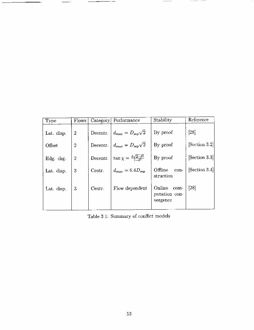
Type
Lat. disp.
Offset
Hdg. chg.
Lat. disp.
Lat. disp.
Flows
2
2
2
3
Category Performance Stability Reference
Decentr.
Decentr.
Decentr.
Centr.
Centr.
dm_x = Ds_pv/2
dm=x = D,epx/2
av%_tan)/= a---Szg-a
dma_ = 6.4D,_p
Flow dependent
By proof
By proof
By proof
Oittine con-
struction
Online com-
putation con-
vergence
[28]
[Section 3.2]
[Section 3.3]
[Section 3.4]
[28]
Table 3.1: Summary of conflict models
53

54

Chapter 4
Control of a linear flow under
separation and schedulingconstraints
4.1 Background
This chapter investigates the problem of propagation of delays in the NAS. The
limited capacity of a runway in bad weather conditions is often the origin of rate
restrictions in the en-route airspace. Aircraft going to that particular runway are
impacted sometimes very early in their flight as restrictions tend to spread easily in
the system (see Section 1.1.2). Fig. 1-3 illustrates a problem that occurred when
restrictions for aircraft inbound to Newark airport impacted traffic hundreds of miles
away in a short amount of time (see [39]).
To delay the propagation of restrictions to upstream sectors, real-life controllers
use a number of different tools (see [40]). One tool is speed control: by slowing down
an aircraft, it is possible to increase the distance from the preceding aircraft, and thus
decrease the sector's apparent output rate of aircraft. This works for a limited period
of time since the aircraft cannot fly below a certain minimum speed. Another tool
is path stretching, whereby the controller increases the distance flown by an aircraft
in his sector to delay the exit. Path stretching is also limited in time because of
geometric constraints of the sector.
Aircraft arrivals scheduling and sequencing represent an increasingly challenging
task, sometimes addressed by automation tools at the ATC facility. Ref. [14] set the
basis for most of the research in Air Traffic Management. Delay propagation in the
NAS is the object of a few studies, such as [4]. Ref. [7] treats the problem of conflict
resolution under scheduling constraints. We choose to analyze scheduling issues at
the sector level to derive macroscopic trends. Some of the issues mentioned thereafter
also appear in the management of other types of transportation. (see [34, 41] for road
traffic applications)
This chapter investigates the behavior of one sector that uses the control schemes
mentioned above to meter its aircraft. Variables of interest are sector length D and
55

width w, speed range, and rate restrictions.
Our metrics are the capacity of the sector and the responsiveness to an output
rate change. This provides a performance index for the control schemes we consider.
We complete the definition of capacity found in Section 2.4.2 as follows: it is the
number of aircraft that have come in at a rate A and have come out at the restricted
output rate #_ after speed control. Responsiveness is the time between a change of
the output rate restriction #r and the change of the actual output rate # as seen byan observer at the exit of the sector.
Section 4.2 introduces the models used for the sector and the aircraft. Section 4.3
presents the control laws to be used to schedule aircraft, and simulations are per-
formed in Section 4.4. Section 4.5 analyzes and derives results of capacity and per-
formance of the global control scheme.
This chapter presents results that appeared in [10].
4.2 System definition
This section describes the models used for the analysis:
kinematics, and aircraft flow behavior.
sector geometry, aircraft
4.2.1 Sector geometry
The en-route sector of interest is modeled by a rectangle, and trajectories are re-
stricted to be two-dimensional (see Section 2.1.3). In the study of speed control, this
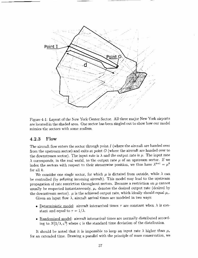
rectangular geometry can be further simplified into a one-dimensional sector: Fig. 4-1
shows that sectors close to major airports match this one-dimensional model. In the
real-world, a lot of sectors also have minor crossing traffic requesting separation: this
is not taken into account in our study. (see [7] for an analysis on this matter)
Our sector is a rectangle of length D and width w, with aircraft arriving at x = 0
(entry point I) and leaving at x = D (exit point O). Fig. 4-1 shows that most sectors
have a length a lot larger than their width. This length D is typically 150 nm in the
National Airspace System and the width w is 40 nm. Points I and O represent the
fixes where flights are handed over from one sector to the next (Fig. 4-1).
4.2.2 Aircraft
Aircraft are modeled as massless points that perfectly follow speed commands. No
dynamics are modeled, and speed changes occur instantaneously. Each aircraft Ai
is associated with a state-vector position-speed (xi, vi). Aircraft fly within a certain
speed range due to buffeting speed limitation on the lower end and maximum Math
number on the upper end: vi 6 [Vmin, Vmax].
Important times in the aircraft journey through the sector are the entry and exit
times, denoted ti and si, respectively.
56
/
Figure 4-1: Layout of the New York Center Sector. All three major New York airportsare located in the shaded area. One sector has been singled out to show how our model
mimics the sectors with some realism.
4.2.3 Flow
The aircraft flow enters the sector through point I (where the aircraft are handed over
from the upstream sector) and exits at point 0 (where the aircraft are handed over to
the downstream sector). The input rate is )_ and the output rate is #. The input rate
corresponds, in the real world, to the output rate # of an upstream sector. If we
index the sectors with respect to their streamwise position, we thus have Ak+l = #k
for all k.
We consider one single sector, for which # is dictated from outside, while A can
be controlled (by refusing incoming aircraft). This model may lead to the upstream
propagation of rate restriction throughout sectors. Because a restriction on # cannot
usually be respected instantaneously, #_ denotes the desired output rate (desired by
the downstream sector), p is the achieved output rate, which ideally should equal p_.
Given an input flow )_, aircraft arrival times are modeled in two ways:
• Deterministic model: aircraft interarrival times T are constant when A is con-
stant and equal to T = 1/A.
• Randomized modeh aircraft interarrival times are normally distributed accord-
ing to N[1/)_, _2] where ; is the standard time deviation of the distribution.
It should be noted that it is impossible to keep an input rate _ higher than #_
for an extended time. Drawing a parallel with the principle of mass conservation, we
57

have "aircraft conservation" in the sector: in steady state, there must be as many
aircraft entering as aircraft leaving. We assume this sector is an en-route sector, and
thus has no airports to act as "sinks" of aircraft.
4.3 Control laws
This section analyzes the various control schemes from basic kinematics. In Sec-
tion 4.3.1, these laws are inquired from a "black box" perspective, regardless of the
type of control. Section 4.3.2 describes the back-propagation process at the level of
the individual sector.
Section 4.3.3 investigates the implementation of the schedule from Section 4.3.1
with speed control. Two variations of speed control are investigated in our study.
As both are based on the same principle, only the first is extensively described. The
second is a simple and straightforward modification of the first. Finally, Section 4.3.4
analyzes the implementation of the desired schedule with path stretching.
We implement a First-In, First-Out control scheme, so that aircraft are not allowed
to overtake one another.
4.3.1 Scheduling
The problem of buffering an aircraft flow in a sector can be seen as a scheduling task.
It consists in scheduling the aircraft exit times to match an output rate limit, although
the input rate has another value. Constraints are of different nature: distance, time,
rates, and speed constraints are imposed simultaneously. Frequent conversions be-
tween those types of constraints thus appear in the derivations.
An aircraft enters the sector at ti and exits at s_. The time it spends in the sector
is ri, where ti + r_ = si. The apparent longitudinal speed is vi = D/ri.
Let us first derive the desired (scheduled) time of exit si. This is subject to three
types of constraints, ordered by priority:
• Aircraft physical capacity: the two aircraft operational speed constraints (Vmin
and Vmax), Eq. (4.1) and Eq. (4.2);
• Regulatory constraint: the separation constraint (minimum separation of Dsep), Eq. (4.3);
• Traffic management constraint: output rate p_, Eq. (4.4).
Following the same order, we have:
8i
D<_ ti +-- (4.1)
Vmin
Dsi >_ ti + -- (4.2)
Vft_ax
Dsep8i >__ 8i_l-JF - (4.3)
Vi-1
1si = S__l + --. (4.4)
58

Thus, the scheduledtime of exit si is:
min ti ÷ --, max t_ + --, si-1 + --, si-1 + • (4.5)Vmin Vrnax Vi- 1
A special note should be made here for the separation constraint. The scheduled
time of arrival derived from the separation constraint Eq. (4.3) only guarantees sep-
aration at exit. However, separation has to be maintained throughout the sector.
Eq. (4.3) is sufficient to guarantee this separation, given that aircraft enter the sector
already separated. Let us denote e the distance between two consecutive aircraft. If
both aircraft keep their respective speed constant, then e varies linearly with time. If
separation is guaranteed both when the speed command is given (by assumption) and
when the aircraft exit Eq. (4.3), then it is assured by continuity anywhere inbetween.
Thus Eq. (4.3) is sufficient to assure separation at any point of the flight within the
sector.
Since each optimal exit time depends on the exit time of the preceding aircraft,
si needs to be determined recursively. For speed control, the speed command is then
derived directly from si with v_ = D/(si -h).
4.3.2 Input rate control
When the sector is unable to deal with an output restriction, it may either decide to
violate the output restriction or request a lower input rate from the upstream sector.
The latter option is considered here.
Various ways to request a lower input rate are possible. ")C could be requested
to be well below, exactly equal to, or slightly above (but then for a limited time) the
imposed output rate #_. We choose to decrease this input rate - that is, the output
of the upstream sector - to the output restriction when minimum speed is reached.
Before that, no restrictions exist.
This strategy back-propagates the restriction as late in time as possible. This is
a relatively tougher restriction than if the restriction is back-propagated right from
the start.
4.3.3 Speed control
We now look specifically at the speed control scheme, under two of its variations:
• Entry control, where aircraft are controlled only once - at their entry - and keep
the commanded speed setting until they exit;
• Extended control, where aircraft speeds are continuously controlled in the first
100_f% of the sector. They keep the last setting in the last 100(1 - "/)% of the
sector.
59

Entry control
In the entry control law, the control system commands incoming aircraft speed on
entry only. This speed setting is not be modified until the aircraft exits.
We consider the four constraints stated above by priority:
• Speed must remain in the operational range of the aircraft: the actual vi is
given in Eq. (4.9).
Separation must be maintained throughout the sector: this requirement can be
verified by only enforcing the separation constraint at the exit with a speed
command vS: Eq. (4.7).
An ideal exit time enforces the desired output rate #r. The speed is adjusted in
Eq. (4.6) to v r so that maximum emciency is achieved, meaning that all aircraft
pairs are exactly a time 1/#_ apart at the output.
Of the last two constraints, the most important is separation: the speed to be
commanded to the aircraft must never be higher than that computed in Eq. (4.7),
yielding v m in Eq. (4.8).
All these requirements translate into the following constraints:
Dv _ = (4.6)
D-xi-1 _.[_ ! 'vi- 1 I_r
D (4.7)v s = Vi-lD+Dsep_Xi_l,
v m = min(v _,vs), (4.8)
vi = sat vmO_(Vm_ (4.9)Vmi n \ I"
where the saturation function is defined as:
sat ba(x) = a for x < a (4.10)
= xfora<x<b (4.11)
= b for x _> b. (4.12)
vi is the speed command effectively passed on to the aircraft. A system diagram
appears in Fig. 4-2 (top), where measured parameters are shown.
Extended control
In this second strategy of speed control, aircraft are submitted to the controller's
command while they are flying over the first 1007% of the sector. The output rate
restriction #_ is only allowed to be piece-wise constant: the speed commands change
60

k- 1 Sector k
Input ]corn_and [--
ra_aratlon
Controllerforsectork-1
Sector k- 1
o Rate• Speed• Separation+ Speedvariation
Input rate
request
-- Outputconstraint]
Controllerfor _ Output rate jsectork c0nstratnt
Controllerforsectork+l
Sector k + 1
>
>
Airspace capacityconstraint
o Rate
• Speed• Separation
_ _ _+Speedvariation
Sector -l t <--t---- tork÷l_-_-_ ] _ SeCtor k ----'_ _'_
. rate, | _ separationI-- Outputconstraint]
Controllerfor LLJ Controllerfor _r Outp_t rate l ' Controllerfor ..., [
sectork-1 I_'_ ] sector k [_'_ constraint sectork+l _,iAirspace capacity
] [ ] constraint
Input rate
request
Figure 4-2: Diagram of the system. Measured parameters are represented with color
markers consistent with those shown on plots. Top: Entry control. Bottom: Setup
of the extended control law, which includes the possibility to control a portion "y of
the sector.
61

only during the step changes of #_. The same requirements as in the previous para-
graph apply, leading to the following system of equations:
v_ = D- x_ (4.13)D-xi-1 nt- 1'
_)i--1 JAr
D - xi (4.14)V s
= vi-1D + Dse p - Xi_ 1
V TM = min(v T,v_), (4.15)
vi = sat vma_(Vm) (4.16)Vmi n \ 1"
If xi C [0, vD] then vi is the speed command given to aircraft Ai when #r changes.
If xi C ]_,D, D] then the speed setting is the last command given to aircraft Ai in
[0, _D].
As the information relative to the output rate restriction is influencing the speed
of aircraft further into the sector, the responsiveness of the sector to a change in #r
is expected to be better than for entry control.
Fig. 4-2 (bottom) gives an overview of the extended law.
4.3.4 Path stretching
We now address the scheduling problem stated in Section 4.3.1 using path stretching.
This approach follows the example of today's air traffic controllers, who usually extend
the path of aircraft to slow them down.
Principle
Path stretching consists of deviating the aircraft by an angle X1 for a time _), and
taking the returning angle X2 for a time _ = ti - s_ - ¢1. Our path stretching
maneuver is restricted to two legs. More legs could be considered, which would lead
to more control authority at the expense of analytical simplicity. Path stretching
is symmetrical if _ = _ (and X1 = -X2). The heading changes are assumed to
be instantaneous, as by Section 2.1.2. (see Fig. 4-3). For all cases, the following
constraints exist (the aircraft exits at one only point):
_) sin X1 = _2 sin X2
D = v(_/lcosx1 +_cosx2).
Performance gain with path stretching
A straightforward analysis shows that path stretching induces an apparent (projected
on the straight trajectory) speed modification of:
A__V_V= 7"1 COSX1 -t- T2 COSX2 _ 1, (4.17)V TIJVT2
where _-1 and 72 are the times spent on each of the two legs of path stretching. To
limit maneuver amplitude, only a certain range of X'S should be used.
62

CJ
W
r
D
Figure 4-3: Path stretching: notations and corner point locus
Symmetrical path stretching
We first consider the case of symmetrical path stretching (_ = _, thus X1 = ;g2 = X).
Here, the largest lateral deviation from the original path occurs at t_ + _, i.e. at the
corner point C in the middle of the trajectory between the entrance and the exit (see
Fig. 4-3). Given w, the width of the sector, and D, its length, the maximum allowabledeviation is:
wtan :gmax = --. (4.18)
D
Eq. (4.17) simplifies to:
and
Z2kV-- = cos ;_- 1 (4.19)
v
Av D - x/D 2 + w 2
v v/D 2 + w 2
Typical values of D (150 nm) and w (40 nm) give Av/v _ -3.4%.
(4.20)
Asymmetrical path stretching
Contrary to the preceding section, we now consider the case where X1 _ X2. From
Eq. (4.17), the locus of corner points of trajectories with identical Av/v is found
to be an ellipse. Fig. 4-3 shows that the use of asymmetrical path stretching helps
achieve the same Av/v with less lateral deviation (the blue trajectory in Fig. 4-3 has
its corner point C beyond the width limit of the sector, while the red trajectory, of
the same length, has its corner point C' within the limits). We choose the minimal
X1 that achieves the requested Av/v.
Fig. 4-4 (right part of the curve) shows the angle X as a function of ,&v/v for a given
D and w (typical values used in the previous section). Efficiency of a control scheme
is measured by the inverse of the slope of the curve, representing the incremental
angular deviation needed to slow down the aircraft by an incremental amount of Av/v.
The asymmetrical path stretching scheme is thus less efficient than its symmetrical
counterpart.
63

path stretching
(Z 1)
Symmetricalpath-stretching
(x)
/
-o.0_ -o._4 _ -o.o3 -0.02 -o.ol o
_=twlv
35
3O
25
2O
15
10
"o
Figure 4-4: Deviation angle X (or X1) as a function of the apparent decrease in
(projected) speed Av/v = _, for a sector of length D = 150 nm and width w = 40 nm.
The function is continuous and consists of two parts, noticeable by the discontinuity of
the slope at Av/v = _t _ -3.4%: the left part is when symmetrical path stretching
is used, and the right part is when the upper limit on width (w) is reached and
asymmetrical path stretching is enforced.
64

W
W
D •
Figure 4-5: Snapshot of a sector under path stretching flow control. Sector length is
D = 150 nm and width w = 40 nm. Trajectories are shown in dimmed lines. Top:
Symmetrical path stretching. Bottom: Asymmetrical path stretching.
General result for path stretching
Fig. 4-4 shows the general result regarding path stretching. The function X(_), with
= Av/v, is the following:
• for _ < _z'w
- arctan (4.21)
-D q- V (_+1)2_(_+2)
• for _ > sol:
arccos (1 + {) (4.22)
with _l - _ 1. This result does not take into account separation, which isinvestigated in the next section.
Path stretching and separation
Because path stretching uses a second dimension by moving the airplanes on a plane,
separation becomes a harder issue than in the speed control case, where timing con-
straints guarantee separation. Fig. 4-5 shows snapshots of a sector using path stretch-
ing for flow control; both symmetrical and asymmetrical cases are shown.
The variation of the distance between two aircraft in line, A1 and A2, is investi-
gated (t2 > tl, i.e. A1 is the first aircraft):
xi(t) = (v(t -- ti) cos Xi, v(t - ti) sin Xi). (4.23)
65

Denoting At = ti+l - ti, and noticing that the entry separation between two
aircraft is:
vAt = D_ev + B (4.24)
where B is the extra buffer between aircraft at entry, we derive the distance e(t):
[(t) = (l)t(cos)/2 -- COS )/1) -- (Dsev + B) cos X2) 2 (4.25)
+(vt(sin X2 - sin )/1) - (D_p + B)sin X2) 2.
e is an increasing function of time when )i2 > X1, which is the case when a restriction
exists (see Fig. 4-4, when _ is decreasing, X is increasing) so that there is no loss of
separation on the first leg of the trajectory. For the return leg, the distance between
the two aircraft decreases. However, they are separated a priori by the choice of
- thus of )/ - which takes into account separation at the exit. Since they are
separated at the corner point, and are separated at the exit, then by monotonicity
they are separated throughout their first leg. Thus, when a restriction exists, no
loss of separation occurs, regardless of the initial separation (larger than Ds_ v by
assumption).
It is different when the restriction has been lifted, and the recovery process is
under way. The minimum distance may then be violated. To solve this problem, the
following policy is implemented: every other aircraft scheduled during the recovery
process is sent on the lower part of the sectoP, in a zone that has not been used
before. Therefore, we ensure a virtual separation at entry equal to 2Dsev. The
following proves that this separation is sufficient to avoid any separation problem.
Using this policy, we have B = Dsep. We find the minimum of e:
(min = mine(t) = D_v_/2(1 + cos )/l COS)/2 + sin )/l sin )/2), (4.26)t>0
which is always larger than D_ep as long as ()/1,)/2) • [0,7r/2] 2. This proves our
previous claim on separation for the first leg. With arguments analogous to those
used previously, separation is also guaranteed on the second leg.
Analogy with speed control
Preceding sections show that path stretching gives results similar to speed control
from the scheduling point of view. Specifically, as the path stretching command is
only given once, and is not modified while the aircraft is in the sector, it is analogous
to entry control.
In the case of speed control, scheduling is respected as long as the lower speed limit
is not reached. With path stretching, scheduling is respected as long as geometrical
limits are not reached. These limits are derived in Section 4.5.3.
Simulations of some restriction scenarios follow. They have been computed using
only speed control. The performance results are analogous to those obtained with
path stretching.
1This policy can be used all the time, we only need it during the recovery process.
66

4.4 Simulations
Simulations of the system using speed control are run under Matlab. In all exam-
ples below, the sector of interest is 150 nm long, consistent with today's National
Airspace System design. Airspeed ranges from 400 kt to 500 kt (see Section 2.1.2).
Appendix A provides a summary of all simulations parameters shown below. To de-
rive simulations for path stretching, this range could be adjusted and derived from
geometrical considerations.
A number of parameters are monitored as functions of time. Fig. 4-2 (top) shows
a concise view of the system, including the points where parameters are measured.
The following section details the plotted values.
4.4.1 Simulation parameters
Simulation results are shown with three different plots (see Fig. 4-6 below for illustra-
tion). The top plot shows the speed given to the aircraft at the entrance of the sector
(one blue dot per aircraft) and the speed at the exit of the sector (purple circles).
One data is not a simple translation in time of the other, because an aircraft flying at
400 kt takes more time to pass through the sector than an aircraft flying at 500 kt.
One way to read this plot is to see the two lines as representing the range of speeds
of the aircraft within the sector. For instance, at t = 2 hr in Fig. 4-6, aircraft in the
sector have speeds ranging from 415 kt to 465 kt, approximately.
The middle plot shows a number of different rates of aircraft (i.e. the number of
aircraft going through certain points over an hour): the dotted green line represents
the input rate A from the upstream sector (sector k - 1 as labeled in Fig. 4-2), the
solid red line the restriction PT on the output flow as requested by the downstream
sector (sector k + 1). The blue dots represent the actual output rate #. These dots
turn to stars if the rate is in violation of the output constraint. However, because in
this model we "flush" the first few aircraft, some blue dots appear as being above the
red line: they represent the "flushed" aircraft.
The bottom plot shows two different things: first, with blue dots, the separation of
aircraft at the exit is shown. This separation, in nautical miles (nm) should never be
below 5 nm. If the separation is greater than or equal to 5 nm at the exit, Section 4.3.3
shows that the separation between aircraft is also above the safety minimum during
the whole time within the sector. Finally, a graph consisting of green crosses shows
the difference in speed of two consecutive aircraft.
4.4.2 Sector saturation
Deterministic arrivals - Entry control
In this first simulation (Fig. 4-6), we test the endurance of the system when an
output restriction lower than the input rate lasts for a time long enough to witness a
saturation of the system.
67

500
g
_5oO3
400
Speed range=400-500 kt, Input=52-52 ac/hr. Restriction=46-60 ac/hr, D=150 nm
*°'*%°° _%%%%
% °%
"%°° %%%
"*%°°.•. %°%%%
°'°°,.°°°,, ........ _ ,, ,,,.
15 2 2.5 3 35
i
At entry JAt exit
65
@o_s-_on."
45
g
_5v
o
03
' ' =, Output i
-- Output constraint I
I ,_put I
................................................i........................1I
i 1 i1 5 2 2.5 3 3.5 4
' ' , Separation at exit I............... J I_'s_e_lat exit ]
"*'"°*'o.,.,,.., ....... ,,,, .......................... ***,_ .......... .., ........ o.°,
i i• °°.o. .....
1.5 2 2.5 3 3.5
Time (hr)
Figure 4-6: Simulation with deterministic scheduled arrivals. A restriction is imposed
on the output rate at t = 1.5 hr.
The situation is initially at steady-state with 52 aircraft arriving per hour ()_ = 52)
at a speed of v = 500 kt, thus creating a spacing of v/A = 9.6 nm. The output
restriction is set to #_ = 60, thus above the input rate )_ (i.e. no restriction is
imposed). There is no speed command given to the incoming aircraft.
At t = 1.5 hr, the output restriction goes below the input rate at #_ = 46, trigger-
ing the need for speed control of incoming aircraft. Arriving aircraft are slowed down
and any new aircraft goes slower than those preceding. This control only impacts the
output rate after the time needed for the first impacted aircraft to reach the end of
the sector, approximately t = D/v = 18 min (our measure of responsiveness). Prom
there on, the output rate matches the output rate constraint until the speed command
reaches an unacceptably low level (vmi,_ = 400 kt). When this level is reached, the
new incoming aircraft are only given the command to slow down to vm_, in order
to maintain spacing. The output # rate returns to A (all new aircraft are given the
exact same speed when entering, thus their output time spacing remains their input
time spacing), and the output restriction is violated.
Deterministic arrivals - Entry and input rate control
One option to avoid violating the restriction is to back-propagate it to the upstream
sector and impose a lower input rate at some point in time (see Fig. 4-7): this mimics
what is done in the real ATM world. Section 4.3.2 describes the control scheme
68

5OO
_so03
4OO
65
._.6O
_on"
45
Speed range=400-500 kt, Input=46-52 ac/hr, Restriction=46-60 ac/hr, D=150 rim, Input control=onli , i
,,_=_o_,.0o_o,Wvz_,_oo I • At entry"o o
"" %%o_ I o At exit
l I l I I
1.5 2 2.5 3 3.5 4
.o..ooo.......o.o.,°.o,_...,,o.o°..o.°o
i i
l out0u,r-- Output constraintInput
_- Violations
' ' i ' i1.5 2 25 3 35 4
b
<_.=
E5
¢n 1.5
, i t i i /o....o.
'*'°"°'°"'"'......°o.........o...o. .............................. o........................
J . Separation at exitIAspeeal at exit i
2 2.5 3 3.5 4
Time (hr)
Figure 4-7: Simulation with deterministic scheduled arrivals. A restriction is imposed
on the output at t = 1.5 hr. Input control is active and lowers the input rate att_ 2.2 hr.
implemented and shown in Fig. 4-7.
Because the input rate exactly matches the output rate, speed control is unneces-
sary and impossible, thus prohibiting the speed of the flow to build up again. To see
the speed command increase, one needs some extra time spacing, provided either by
a lower input rate or a higher output rate (the latter is possible when the restriction
is lifted).
Randomized arrivals - Entry control
Fig. 4-8 presents a simulation analogous to that of Fig. 4-6, except the arrival process
is now randomized. The random variable here is the time between two successive
arrivals. This inter-arrival time is normally distributed with a mean equal to I/A,
with A appearing on the plot as a dotted green line, and a standard deviation q -- 5
s. Approximately 95_ of all inter-arrival times occur in [I/A - 2q; I/A + 2_].
The capacity - defined as the number of aircraft passing through the sector and
able to match the desired output constraint - is not much impacted by the randomness
of the arrivals. Multiple runs of simulations with randomized arrivals have shown
that the average capacity remains constant for different values of g, as long as the
randomness does not imply a violation of the minimum separation constraint at the
entry.
69

5OO
v
_5o¢3Lcq
400
7O
'C"
¢b
po
g
Speed range=400-500 kt, Input=52-52 ac/hr, _ =5 s, Restriction=46-60 ac/hr, D=150 nmi
At entry IAt exit°°% %°
%. %o o
°%. °%°°° _%
°% %°
I I I
1.5 2 2.5
I I
3 3.5 4
i.ou u,iOutput constraintInput
_, Violations1 • *** " * 1
".-.... ._'.... **** ,_ _* * _' ** **** /•' • "" "1 " ." ** .***., *** ** "* _ ** _**_i _,, J
I " - ...... i ..... I" I " I " /
1.5 2 2.5 3 3.5 4
...... T..... I i I I J
_'I0 '-" ......"'...." ....'.".'.....'."-."';;";;"; ............. i_'_,,_._ ................... +.... . ,_ "°'°°°°°°°° "°°°',°°°°o°°" °°° "'°o'..°o°°°°'°°°°°°°° °°'°°.°° °°'°'°°° °°°°°°"o.°°°°°°°"
..,°,_ .......... ,.......... , . • Separation at exit"+' + ' + +/- 3 _ bound (unctrld arrivals only)
+ + , ]Aspeedlat exit
_" 1.5 2 2.5 3 3.5 4o3Time (hr)
Figure 4-8: Simulation with randomized arrivals. A restriction is imposed on the
output at t = 1.5 hr.
Deterministic arrivals - Extended control
In the operational environment, an output restriction might be imposed by the down-
stream sector with short notice. The goal is then to match the desired output rate in
the shortest time. To improve the responsiveness of the system (equal to t = D/v in
the entry control scheme), we consider controlling the first 1003,% of the sector (Fig. 4-
2 bottom). It is impossible to control 100% of the sector because this might imply
dramatic speed changes close to exit. Furthermore, the assumption of instantaneous
speed change does not hold in such a case.
Fig. 4-9 shows a simulation using this particular algorithm, with 1007 = 80% of
the sector controlled. The responsiveness is improved. Straightforward analysis tells
us that the 20% of the sector not under control translates into a delay of t = (1-_)D/v
(or approximately 4 min) before the restriction is met. This is better than the result
obtained with entry control (18 min).
The speed evolution with time is different. The speed curve at exit from t __ 1.6 hr
to t -----1.8 hr has a particular shape (compare Fig. 4-9 with Fig. 4-6). It reflects the
speed commands given to the aircraft already in the sector when the restriction is
imposed. Once those aircraft are flushed, the usual variation returns.
An interesting property appears when modifying the parameter 3'. The capacity
of the sector remains unchanged for a wide range of 3'. We assume here that the
speed commands given to aircraft within the sector at the issuance of the restriction
7O

5O0
A
_5o
Q.co
4OO
65
@o
_5._orr"
45
_2_D
_s
_o(D
co
Speed range=400-500 kt, PartCtrld=80%, Input=52-52 ac/hr, Restriction=46-60 ac/hr, D=150 nmI I I I u
At entryAt exit
%°-o.,,_o.%% 1
°'%'"%,%,. %%%%%%_
""....... ;......... :_-- I I
115 2 2.5 3 315 4
I I i
-- Output constraint I
Input I• Output.......................................................... I * Violation
i '1 5 2 2.5 3 3.5 4
I I
• Separation at exit
I,_speedlat exit
'•°°°°•°°°°°°°°•° .......... : ........ ° ...... °•°°°'°°°'°°°'•°°°o°•° ........ °°°°°ooo°°°°°oo.°o°•o ....... ° ........ oo.°oo.°°°°o..°°.4°.°.°°oo.°°oo ......
1.5 2 25 3 3.5 4
Time (hr)
Figure 4-9: Simulation with 80% of the sector controlled. A restriction is imposed on
the output at t = 1.5 hr.
is in the acceptable range of speed (i.e., greater than vmi_). Controlling a greater
portion of the sector only improves responsiveness. This is of great interest from an
Air Traffic Management perspective. An analysis is given in Section 4.5.2.
4.4.3 Temporary restriction
After a restriction has been present for some time, and this restriction has been lifted
to a value higher than the input rate, speed commands should be driven back to their
original value (here v = 500 kt). However, two parameters influence this recovery
process: the minimum separation distance between aircraft must be respected as well
as the new output rate (Section 4.3.3).
In the following simulations two modes of recovery are identified: one where the
output restriction is the limiting factor, and another where the minimum separation
distance is.
Fig. 4-10 shows a simulation where the output rate drives this recovery: the speed
command is high enough, so that aircraft are time-spaced at the output at the lowest
value admissible for the given output rate (here: #_=60). Separation remains above
the 5 nm limit, and thus does not constitute a hard bound.
Fig. 4-11 shows a simulation where speed commands are given so that the 5 nm
spacing is respected throughout the sector. If speed commands were given only based
on the possible output rate, this separation would have been violated. Thus, the
71

s00!
psoC3.O_
4OO
65
_s_ot't"
45
oCO
Speed range=400-500 kt, Input=52-52 ac/hr, Restriction=46-60 acJhr, D= 150 nm
i ,,o,o,._,oo,,o=.4_
"%°%°°%. %%% _ °" °° °° _¢o°_
% % °° _,,
%.° _ _
"°°°%°°°.°°° _°%%%_ o_°
I • At entryAt exit I
J I 1 l I
1.S 2 2.5 3 35 4
,15 2:5
i ..... .t
j Output I
-- Output constraintInput
_ Violations3 _.o a
To.,., .......... ,o.....,,,.. .......... °,o'''"°'_"*'*.O.o_.°..,°, ...............:.........................'........................,4"" ...... 1 " Separation at exit
IAspeeal at exit II
J
l l I I
1.5 2 2.5 3 3.5 4
Time (hr)
Figure 4-10: Simulation with deterministic scheduled arrivals. A restriction is im-
posed on the output at t = 1.5 hr and returns to 60 ac/hr at t = 2 hr.
actual output rate is lower than the maximum allowed.
4.4.4 Finite acceleration
Contrary to the rest of this thesis, we now consider aircraft with a finite acceleration
capacity. This simulation will not lead to an analysis and is only meant to provide
a ground for comparison with massless aircraft models. We build on the simulation
found in Fig. 4-9 that addresses extended control of the sector. The exact same pa-
rameters are used, except the acceleration and deceleration that are set at =1=0.4kt/s.
This is an acceptable figure found in Air Traffic Control manuals [31, 13].
For such a value, differences between the purely kinematic and this enhanced
model are barely observable (see Fig. 4-12). Noticeably: no loss of separation occur,
and the capacity is cut by 10% aircraft (3 out of 32). This decrease of capacity is a
direct consequence of the limited acceleration: for an equivalent aircraft in both mod-
els, the commanded speed needs to be lower to counterbalance the distance accrued
while flying faster than desired during the deceleration phase. Thus, an aircraft takes
more of the "speed reserve" and this reserve is exhausted earlier than in the purely
kinematic case, yielding a lower capacity.
The restrictions imposed here are not very tough (reduction of only 12% of the
capacity), and do not require dramatic speed changes. Further simulations should be
run to better understand this problem.
72

500
g
o.O3
4OO
100
8o
__6o
Speed range=400-500 kt, Input=52-52 ac/hr, Restriction=46-96 acJhr, D=150 nm
i i t v i
""'"'.., '°°'°%°oo • I ° AtAtexitentry
i I i I I15 2 25 3 3.5 4
1.5
Q. I
1.5(f)
ou,ou,:L-I: -- Output constraint I
I input /Violations _ J
...............' ............................Z ...................L
2.5 3 3.5 4
i i , i i i /
........... •• ................. • ......... °'•"••'°.,,,•,o.°, ..... _ ..• ................ oo•° ............. •• ................. • ........... •o..,o• .....
• Separation at exit
IAspeealat exit
2 2.5 3 3.5 4
Time (hr)
Figure 4-11: Simulation with deterministic scheduled arrivals. A restriction is im-
posed on the output at t = 1.5 hr and returns to 96 ac/hr at t = 2 hr.
4.5 Capacity analysis
We defined and simulated three control schemes: speed control in its two variants
(entry control and extended control), and path stretching. In this last section, we
derive the theoretical capacity of these schemes. We conclude our study with the
capacity obtained when speed control and path stretching are successively used.
4.5.1 Entry control
Capacity computation can be achieved in two different ways in the case of speed
control. One is to use Eq. (4.6) recursively to compute the speed of the n th aircraft
when a restriction #_ is enforced, with a flow initially flying at v/. Once v, is known,
capacity is computed by solving v, = vm_, for n. Closed-form results are not available,
due to the recursive nature of the calculation.
Another way to proceed is to see aircraft as vehicles with scheduled times of entry
and exit. Knowing those two times, speed is easily derived knowing the length of the
sector. We restrict our analysis to entry control only under deterministic arrivals and
extend the result to the extended control case in Section 4.5.2.
The metering constraint #_ is set at time t. Thus, for all aircraft Ai such that
ti > t, the exit time si is set so that si - 8i-1 -- 1/#_. We assume t = t +, i.e. the
constraint is set when aircraft A0 enters. The speed command given to Ao has not
73

Speed range=400-500 kt, Accel=0.4 kt/s, PartCtrld=80%, Input=52-52 ac/hr, Restriction=46-60 ac/hr, D=150 nm
5OO
g_5o(,9
4O0
I I i I I .41_..o.ooo,.oo,,o,, ................................. .o,..,o..,,,o ...... , ........... ,,o.o.,o,,,,.o.o,,,oo,oo,oo,,.,,o,o,, ...... •
[ IAt exit
%%%
%%
I I I I I1 5 2 2.5 3 3.5 4
65
...60
_orr
45
g5
_9
i i I I
-- Output constraint I
/ I Input1 • Output
I "_ .... _ ............. ":'::* I I I
1.5 2 2.5 3 3.5 4
I I
I • Separation at exitIZ_sp_dlat exit
I + I I I
.... o.o,,.o....oo,,°ooo.ooo°_ ....... o. ........ ..Ooo,,ooo
ooo°°oo.°ooooooo.oooooo,o°°oooooo,o,o°°°o°o,,.o°oo°oooooooo ......... oo .............. o.oo.
1.5 2 2.5 3 3.5 4Time (hr)
Figure 4-12: Simulation with an enhanced aircraft model. The acceleration is limited
to 0.4 kt/s. This plot should be compared with Fig. 4-9 as the same simulation
parameters are used: deterministic scheduled arrivals, control over 80% of the sector,
restriction imposed on the output at t = 1.5 hr and lifted.
74

taken into account the restriction #_. Thus:
DSo = t+--
V0
= SD
Sl = t+--Vl
1- +S
n
sn - + S. 4.27)
Also:n
tn = -_ + t.
Combining Eq. (4.27) and Eq. (4.28)"
4.28)
D
Tt 1 __ jr_ v l
4.29)
Equating Eq. (4.29) with Vmin, we can solve for rive, the capacity of the sector
obtained with speed control:
nvc = D(1- ", ) (4.30)
(1--1)As expected, the capacity of the sector depends on the length D, the flow speed vf,
the minimum speed vmi,, and the input and output restriction rates.
4.5.2 Extended control
Section 4.4.2 showed that extended control has the same capacity regardless of "7.
Fig. 4-13 shows a visual proof of that property. The red trajectories are created
by aircraft controlled under entry control only. The restriction is issued at t. From
there on, entering aircraft are assigned times of exit, separated in accordance with p_.
Accordingly, speed commands that are expected to respect these schedules are given.
This lasts until the minimum speed is reached - the minimum speed is geometrically
visualized by a green triangle on the picture.
Black trajectories represent aircraft controlled under the extended law (control
over 1007% of the sector). We notice that the trajectories and scheduled times of
exit are identical. Only the time of issuance of the restriction t _ appears later than for
the previous case, which means it is closer to the time when the metering is enforced
(already noticed with the faster response). Trajectories are identical except for those
which intercept the line representing time t _ (i.e. the aircraft already in the sector
at time t'). These trajectories have "kinks" in them, resulting from the change of
speed given to them at this time. They have the same scheduled times (with another
75
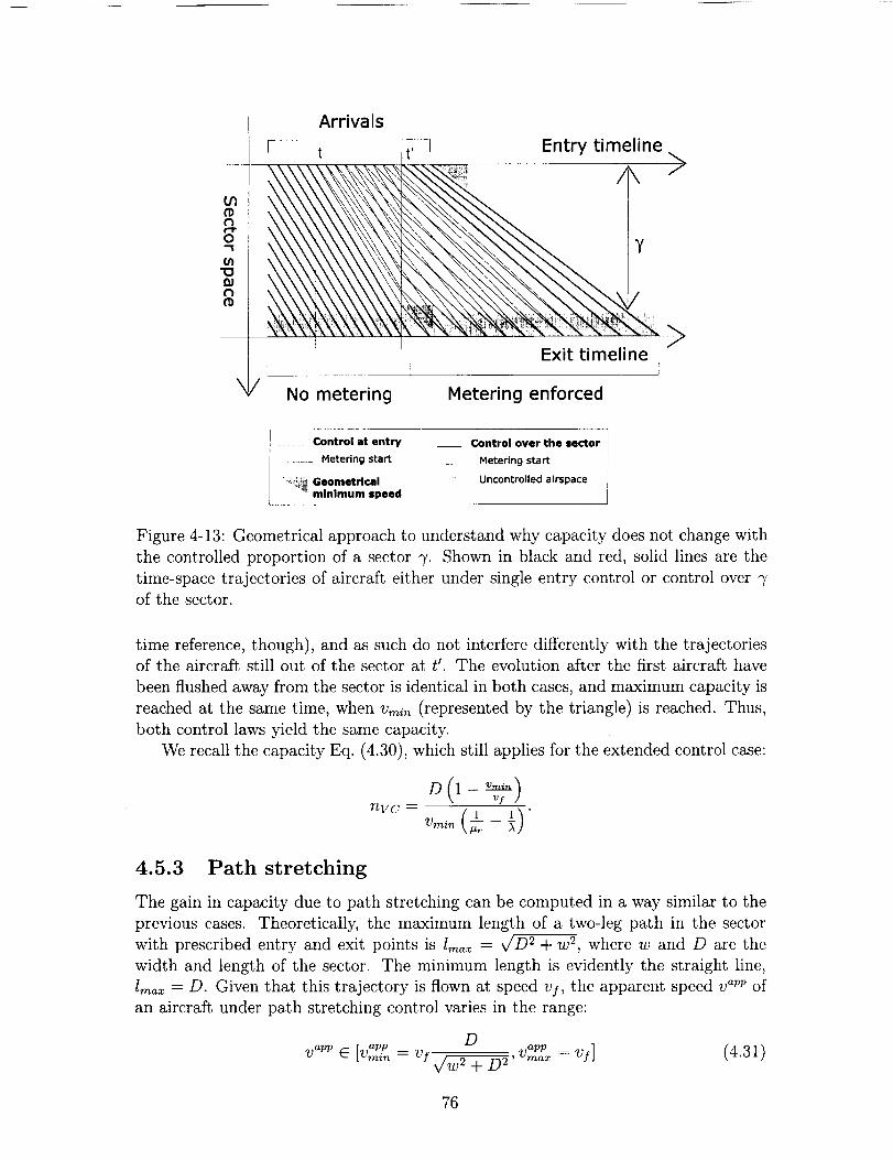
o
ID
Arrivals
[ :t _t' I
/
Entry timeline
\ >
Y
/
Exit timeline
/ No metering Metering enforced
................Control at entry
..... Netering start
_ Geometricalminimum speed
__ Control over the sector
__ Metering start
Uncontrolled airspace
Figure 4-13: Geometrical approach to understand why capacity does not change with
the controlled proportion of a sector 7. Shown in black and red, solid lines are the
time-space trajectories of aircraft either under single entry control or control over 7of the sector.
time reference, though), and as such do not interfere differently with the trajectories
of the aircraft still out of the sector at t'. The evolution after the first aircraft have
been flushed away from the sector is identical in both cases, and maximum capacity is
reached at the same time, when Vmin (represented by the triangle) is reached. Thus,
both control laws yield the same capacity.
We recall the capacity Eq. (4.30), which still applies for the extended control case:
v__mmv,)?_VC =
4.5.3 Path stretching
The gain in capacity due to path stretching can be computed in a way similar to the
previous cases. Theoretically, the maximum length of a two-leg path in the sector
with prescribed entry and exit points is lm_x = v/D2+ w 2, where w and D are the
width and length of the sector. The minimum length is evidently the straight line,
Im_ = D. Given that this trajectory is flown at speed vi, the apparent speed v _vv of
an aircraft under path stretching control varies in the range:
Dr- ,,vv _/,vv = vs] (4.31)
V app _ tVrnin : Vf V/W2 "_- D2,--max
76

We cannow useEq. (4.29),and by equating Vn with" appVmin, we get a capacity for path
stretching:
v/w 2 + D 2 - D
1)A noticeable fact about the latter expression is its dependence on 1/vy. From a
practical perspective, it means that the path stretching "tool" is more efficient with a
lower entry speed. It is then logical to think about sequencing both control schemes
(speed control and path stretching) to obtain an enhanced capacity.
4.5.4 Sequence of control policies
In this last section, we adopt the following procedure:
• No restriction is initially applied to the sector's outgoing rate.
When a restriction occurs, entry speed control is enforced. Airplanes start
decreasing their speed according to their positions in the flow.
Airspeed control authority is lost after nvc aircraft. The th aircraft has speednvc
greater than or equal to vmi_. To transition smoothly to path stretching (at the
beginning of which aircraft do not deviate much from the straight line), aircraft
under path stretching control are given a speed of vmi,_, avoiding any separation
problem.
• Path stretching control authority is lost after nps.
If the restriction is lifted before this happens, the recovery process first involves
sending every other aircraft on the other side of the sector (see Section 4.3.4).
When the apparent speed of the aircraft returns to Vmin, entry speed control
takes over path stretching until a return to normal is effective.
Using this two-scheme procedure, we obtain a sector capacity of:
x/w 2 + D _ _ Dy_=u_v_ (4.33)ntota I =
77

78

Chapter 5
Conclusions
This work considers two aspects of en-route airspace operations, in an idealized fash-
ion. Although aircraft are modeled without dynamics, the maneuvers under con-
sideration lead to nice yet meaningful results of stability or performance of control
policies.
Intersecting flows of aircraft are the object of Chapter 3. Section 3.2 complements
the initial works of Mao [28, 29, 30] on two intersecting aircraft flows and extends his
results to the new, more realistic offset maneuver model. Section 3.3 is an analysis of
the same model where aircraft use pure heading changes to perform conflict avoidance.
In Section 3.4, the problem of divergence of three intersecting flows with decentral-
ized conflict avoidance algorithms is addressed with a centralized, procedure-based
control concept. Comparison with flow-dependent control strategies requiring online
computations shows competitive performance. Future work on this side of the project
should concentrate on extending results of Section 3.3 to aircraft flows intersecting at
various angles and with different speeds in each flow.
Aircraft flow buffering and delay back-propagation in the air traffic system are
modeled in Chapter 4. Simple considerations show how adequate control of a sector
facing input/output imbalance can alleviate the overload of the airspace network by
avoiding unnecessary transmission of delays. Compact performance indices bring
insight as to what capacity to expect in various models. A natural and necessary
extension to that part of the work would be to add the impact of an intersecting flow.
This step would allow the coupling of conflict avoidance and traffic scheduling
constraints. It is a natural way to address the recurring question of airspace sector
capacity and help in the redesign of the air traffic control system.
79
80
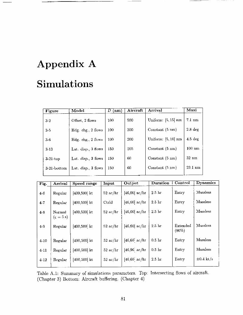
Appendix A
Simulations
Figure
3-2
3-5
3-6
3-13
3-21-top
3-21-bottom
Model
Offset, 2 flows
Hdg. chg., 2 flows
Hdg. chg., 2 flows
Lat. disp., 3 flows
Lat. disp., 3 flows
Lat. disp., 3 flows
D (nm)
100
100
100
150
150
150
Aircraft
500
200
200
105
60
60
Arrival
Uniform: [5, 15] nm
Constant (5 nm)
Uniform: [5, 10] nm
Constant (5 nm)
Constant (5 nm)
Constant (5 nm)
Maxi
7.1 nm
2.8 deg
4.5 deg
100 nm
32 nm
23.1 nm
Fig. Arrival
4-6 Regular
4-7 Regular
4-8 Normal
= 5 s)
4-9 Regular
4-10 Regular
4-11 Regular
4-12 Regular
Speed range Input Output Duration Control Dynamics
[400,500] kt
[400,500] kt
[400,500] kt
[400,500] kt
[400,500] kt
[400,500] kt
[400,500] kt
52 ac/hr
Ctrld
52 ac/hr
52 ac/hr
52 ac/hr
52 ac/hr
52 ac/hr
[46,60] ac/hr
[46,60] ac/hr
[46,60] ac/hr
[46,60] ac/hr
[46,60] ac/hr
[46,96] ac/hr
[46,60] ac/hr
2.5 hr
2.5 hr
2.5 hr
2.5 hr
0.5 hr
0.5 hr
2.5 hr
Entry
Entry
Entry
Extended
(80%)
Entry
Entry
Entry
Massless
Massless
Massless
Massless
Massless
Massless
+0.4 kt/s
Table A.I: Summary of simulations parameters. Top: Intersecting flows of aircraft.
(Chapter 3) Bottom: Aircraft buffering. (Chapter 4)
81

82

Appendix B
Complementary problem
Section 3.3.3 introduced the eastbound protection zone. This area is used in the
stability proof of Section 3.3 to show that it would have contained the projected
conflict zone of the southbound aircraft Aj if Aj had not deviated at all (i.e. rl =
-7r/2). For the sake of the argument, the condition to prove here is slightly different:
if Aj had only deviated by X/2 (i.e. r/ = -7r/2 - X/2), prove that Aj's projectedconflict zone would have been in the eastbound protection zone. This subtlety has
been omitted in the stability proof for clarity of exposure. It does not change the
proof in any way because the contradiction remains: "Aj could have deviated less".
The mathematical problem is exposed below. Explanations for each steps are
given afterwards.
Given 10 < 5 < - (B.1)
-- -- 2
and
we want to prove that for all
there exists a
such that for all
we have:
X = arctan 5V_ - 5 21 - 5 2 (B.2)
X X] (B.3)o e
e.(e) e [-X, X] (B.4)
Al>0andA2_>0
(B.5)
(B.6)
with
A, = -(sin(On) sin(r/) + sin(On) cos(r/) + cos(O,_) sin(r/) - cos(r/) cos(On) + 1 (B.7)
-a v_ Vq + sin(On) sin(r/) - cos(r/) cos(On))/(sin(O,J + sin(r/)) + (-1
X s X X X+cos(T ) sin(O) + co (-_) cos(O) - sin(T ) cos(O) + sin(T ) sin(O)
83

+(sin(r/) sin(O) + sin(O) cos(r/) + cos(0) sin(r/) - cos(r/) cos(0) + 1
-5 _ V/1 + sin(rD sin(0) - cos(r/) cos(0))/(sin(0) + sin(r/))
and
Y 3/ "g )(
A2 : -(-1 +cos(7)sin(0)+cos(2)cos(0)-sin(2)cos(0)+sin(2)sin(0) (B.8)
X sin(0) sin(2)cos(O ) - 1))/(-cos(2 ) + sin(0))+ 7-a 2(cos(7) -
-(sin(r/) sin(0) + sin(0) cos(,D + cos(0)sin(r/) - cos(r/) cos(0) + 1
+3 v_ V/1 + sin(r/) sin(0) - cos(,D cos(0))/(sin(0) + sin(r/))
+(sin(0,) sin(r/) + sin(0,) cos(r/) + cos(0,) sin(r/) - cos(r/) cos(0,) + 1
+3 v_ ql + sin(0.) sin(r/) - cos(r/)cos(0.))/(sin(0.) + sin(r/)).
Eq. (B.1) states that the control volume has to be sufficiently large to enable
conflict avoidance maneuver. In practice, ($ is usually in the order of 0.2 or less.
Eq. (B.2) recalls the result of Eq. (3.10). Aj has maneuvered so that q = -rr/2- X/2:
its projected conflict zone intersects the eastbound decision bound for 0 E [-X/2, X],
yielding Eq. (B.3). Let us consider the "southern edge" of Aj's projected conflict
zone (i.e. a, see Fig. 3-7). We want to show the following lemma.
Lernrna: any eastbound aircraft A_ sitting on this southern edge provides a conflict
free solution for a newcorning eastbound aircraft A, sitting on the eastbound decision
bound with angle On.
Equivalently, this shows that the southern edge is in the eastbound protection
zone. Eq. (B.4), Eq. (B.5), and Eq. (B.6) provide the verification of the lemma.
Eq. (B.8) and Eq. (B.9) are both positive if the projected conflict zone of A, is inside
that of Ai.
One difficulty of this mathematical problem arises from the absence of expression
for 0, (Eq. (B.4) only says: "there exists a 0,"). By curve-fitting, an expression has
been found for 0, and gives a correct 0_ for 5 < 0.2. Given the geometric parameter
5 and the position of Ai described by 0, 0_ is expressed by:
0n = 0M_ r, (B.9)
where
0 = (1 O 02 03 ), (B.10)
a = ( 1 5 52 5a 54 ), (B.11)
-1.731 • 10-5 -0.7062 -0.5177 -0.8154 +0.1876 '_M = -1.942.10 -5 +1.342.10 -a -1.019 -3.a99 +0.6398 ) (B.12)+2.824.10 -5 -3.818.10 -4 -1.396.10 -2 -2.905 -6.63a '-1.101 •10 -4 +9.107.10 -a -0.2543 +2.903 -17.00
84

Appendix C
Nomenclature
Ai = Eastbound or generic aircraft
Aj = Southbound aircraft
A_ = Newcoming aircraft
a = Radial coordinate of a southbound aircraft
B = Additional buffer distance between aircraft
b = Radial coordinate of an eastbound aircraft
C = Corner point
c = Normalized relative speed
D = Distance to point with constraints (radius or length sector)
d = Lateral displacement amplitude
d._x = Maximal lateral displacement amplitude
Dsep = Minimum separation distance between aircraft
E = East point
h = Aisle width
I = Entry pointi = Index
J = Point on the lateral limit of the sector
j = Index
k = Index
M = Matrix of polynomial coefficients
m = Miss distance vector
N = North point
n = Index
O = Intersection or exit point
P = Protection zone
r = Time in sector
S = South point
s. = Exit time
t = Entry time
v = SpeedContinued...
85

W
Ig
X
Y
_1,2
0
#
#r
//
P
(7
T
X
= West point= Sector width
= Cartesian coordinate
= Cartesian coordinate
= Scaled a
= Scaled b
= Portion of sector under control
= Scaled D_ep= Distance between two aircraft
= Time on a path-stretching leg
= Angular coordinate of a southbound aircraft
= Angular coordinate of an eastbound aircraft
= Input rate
= Output rate
= Desired output rate
= Scaled v
= ,Sv/v= Northern edge of the projected conflict zone
= Southern edge of the projected conflict zone
= Standard deviation of interarrival times
= Interarrival time
= Heading change
86

Bibliography
[1] Concept definition for Distributed Air/Ground Traffic Management (DAG-TM).
Technical report, Advanced Air Transportation Technologies (AATT) Project,
September 1999.
[2] Operational evaluation report on ADS-B. Final report, Operational evaluation
coordination group, 1999.
[3] J. Andrews. A relative motion analysis of horizontal avoidance. Technical report,
MIT, Lincoln Lab, 1978.
[4]A. Bayen, P. Grieder, and C. Tomlin. A control theoretic predictive model for
sector-based air traffic flow. AIAA Guidance, Navigation and Control Confer-
ence, AIAA-2002-5011), August 2002.
[5] K. Bilimoria. A geometric optimization approach to air conflict resolution. Pro-
ceedings of the AIAA Guidance Navigation and Control Conference and Exhibit,
Denver, CO, (AIAA-2000-4265), August 2000.
[6] K. D. Bilimoria, K. S. Sheth, H. Q. Lee, and S. R. Grabbe. Performance evalua-
tion of airborne separation assurance for free flight. AIAA Guidance, Navigation
and Control Conference, (AIAA-2000-4269), 2000. Denver, CO.
[7]K.D. Bilimoria and H.Q. Lee. Aircraft conflict resolution with an arrival time
constraint. AIAA Guidance, Navigation and Control Conference, (AIAA-2002-
4444), August 2002.
[8] S. Devasia, M. Heymann, and G. Meyer. Automation procedures for air traffic
management: a token-based approach. Proceedings of the American Control
Conference, Anchorage, AK, May 2002.
[9] S. Devasia and G. Meyer. Automated conflict resolution procedures for air traffic
management. Proc. IEEE Conf. Decision and Control, Dec. 1999.
[10] D. Dugail, E. Feron, and K. Bilimoria. Conflict-free conformance to en-route flow-
rate constraints, to appear in the AIAA GNC Conference Proceedings, Monterey,
CA, (AIAA-2002-5013), August 2002.
87

[11] D. Dugail, E. Feron, and K. Bilimoria. Stability of intersecting aircraft flows using
heading change maneuver for conflict avoidance. Proceedings of the American
Control Conference, Anchorage, AK, May 2002.
[12] D. Dugail, Z.-H. Mao, and E. Feron. Stability of intersecting aircraft flows undercentralized and decentralized conflict avoidance rules. Proceedings of the AIAA
Conf. on Guidance, Navigation and Control, 2001.
[13] P. Dumaitre. ContrSle de la circulation adrienne et technique d'utilisation: le
contrSleur et les performances-avions en approche. Ecole Nationale de l'Aviation
Civile, 2 edition, 1993.
[14]
[15]
H. Erzberger and W. Nedell. Design of an automated system for management
of arrival traffic. Technical Memorandum TM-102201, NASA, June 1989.
E. Frazzoli, Z.-H. Mao, J.-H. Oh, and E. Feron. Resolution of conflicts involving
many aircraft via semidefinite programming. To appear in AIAA Journal of
Guidance, Control and Dynamics, 2000.
[16] G. Granger, N. Durand, and J.-M. Alliot. Optimal resolution of en-route con-
flicts. _th USA/Eitrope Air Traffic Management RD Seminar, December 2001.
[17] J. Histon, C. Aigoin, D. Dalahaye, R. J. Hansman, and S. Puechmorel. Intro-
ducing structural considerations into complexity metrics. _th Air Traffic Man-
agement R_D Seminar, December 2001.
[18] J. Histon and R. J. Hansman. Identification of potential air traffic complexity
factors through field observations at Boston ATC facilities. Presentation at the
JUP quarterly review, January 2001.
[19]
[2o]
[21]
[22]
[23]
[24]
J. Hu, M. Prandini, and S. Sastry. Optimal coordinated motions of multiple
agents moving on a plane. SIAM Journal on Control and Optimization, 2001.
Submitted.
I. Hwang and C. Tomlin. Protocol-based conflict resolution for finite information
horizon. Proceedings of the American Control Conference, Anchorage, AK, May
2002.
H. Idris and R.W. Simpson.
traffic in the terminal area.
Boston, MA, 1998.
New approach to the planning and control of air
AIAA Conf. on Guidance, Control and Dynamics,
ILOG. ILOG CPLEX user's guide. 1999.
J. Krozel and M. Peters. Strategic conflict detection and resolution for free flight.
Proc. IEEE Conf. Decision and Control, San Diego, CA, December 1997.
J. Krozel, M. Peters, and K. Bilimoria.
distributed air/ground traffic separation.
and Control, August 2000.
A decentralized control strategy for
AIAA Conf. Guidance, Navigation,
88

[25]
[26]
[27]
[28]
[29]
[3o]
[31]
[32]
[33]
[34]
[35]
[36]
[37]
J. Krozel, M. Peters, K. D. Bilimoria, C. Lee, and J. S. B. Mitchell. Syetem
performance characteristics of centralized and decentralized air traffic separation
strategies. _th Air Traffic Management R_D Seminar, December 2001.
J.K. Kuchar and L.C. Yang. A review of conflict detection and resolution mod-
eling methods. IEEE Transactions on Intelligent Transportation Systems, 1(4),
2000.
K. C. Lin, A. Sisti, and L. Chow. Study on crowded two-dimensional airspace-
self-organized criticality. AIAA Journal of Aircraft, 35(2):301-306, March-April
1998.
Z.-H. Mao. Stability and performance of intersecting aircraft flows under decen-
tralized conflict resolution. Master's thesis, MIT, 2000.
Z.-H. Mao, E. Feron, and K. Bilimoria. Stability of intersecting aircraft flows
under decentralized conflict avoidance rules. AIAA Conf. Guidance, Navigation
and Control, August 2000.
Z.-H. Mao, E. Feron, and K. Bilimoria. Stability and performance of intersecting
aircraft flows under decentralized conflict avoidance rules. IEEE Trans. Intelli-
gent Transportation Systems, 2(2):101-109, 2001.
M. Martin. Opdrations adriennes, volume 1-2. Ecole Nationale de l'Aviation
Civile, 4 edition, 1990.
F. MSdioni. Mdthodes d'optimisation pour l'dvitement adrian: syst_mes cen-
tralisgs, syst_mes embarqugs. PhD thesis, Ecole Polytechnique, 1998.
P. Mishra and G. Pappas. Flying hot potatoes. Proceedings of the American
Control Conference, Anchorage, AK, May 2002.
K. Nagel, M. Rickert, P. Simon, and M. Pieck. The dynamics of iterated
transportation simulations. TRIannual Symposium on Transportation ANaly-
sis (TRISTAN-III) in San Juan, Puerto Rico, 1998.
W.P. Niedringhaus. Stream option manager: automated integration of aircraft
separation, merging, stream management, and other air traffic control functions.
IEEE Trans. Systems, Man, and Cybernetics, 25(9):1269-1280, 1995.
L. Pallottino, A. Bicchi, and S. Pancanti. Safety of a decentralized scheme for
free-flight ATMS using mixed integer linear programming. In American Control
Conference, May 2002. Accepted.
L. Pallottino, E. Feron, and A. Bicchi. Conflict resolution problems for air traffic
management systems solved with mixed integer programming. IEEE Transaction
on Intelligent Transportation Systems, 3(1) :3-11, March 2002.
[38] R.W. Simpson. Course Notes for 16.72: Air Traffic Control. MIT, 1993.
89
[39] A. Sinha and D. Boone. The anatomy of delays: Complexity and interconnec-tivity of nas traffic flow. Presentation,The MITRE Corp., February 2001.
[40] T. Weidnerand S.Green.Modelingair traffic managementautomationmeteringconformancebenefits. AIAA Progress in Astronautics and Aeronautics Series:
Air Transportation Systems Engineering, 193, 2001.
[41] Q. Yang. A Simulation Laboratory for Evaluation of Dynamic Traffic Manage-
ment Systems. PhD thesis, MIT, 1997.
9O

Stability of intersecting aircraft flows using heading change
maneuvers for conflict avoidance
Zhi-Hong Mao * David Dugail t Eric Feron * Karl Bilimoria §
December 20, 2002
Abstract
This paper considers two intersecting flows of aircraft that must avoid each other.
Considering avoidance maneuvers modeled by instantaneous heading changes, this
paper introduces sufficient conditions for a "domino effect" not to occur, whereby
one aircraft's conflict avoidance action fails to generate cascaded, diverging conflict
avoidance actions. The mathematics involved with the heading change model are
considerably more complex than using simpler, previous maneuver models. However,
this additional effort is largely compensated by the improved realism of the maneuver
model, as well as new insights in the inherent robustness of conflict avoidance maneuver
schemes against real or perceived acceptable separation standards. The analytical
results are compared with simulations.
1 Introduction
The increase of air traffic over the past decades has resulted in increased air traffic con-
troller workload and more frequent airborne delays. However, better navigation, com-
munication and computing technology has made it possible to conceive new concepts of
traffic operations, such as Free Flight, which bear the hope for more efficient handling of
airborne traffic.
The development and subsequent implementation of any new air traffic management
concept of operations requires one to study in-depth the mechanisms by which airplanes
are able to maintain separation from other airplanes at any time and in a predictable
fashion. Several recent efforts have aimed at proposing solutions to automate aircraft
separation by issuing required trajectories to airborne aircraft, either through centralized
*Harvard-MIT Division of Health Sciences and Technology, Massachusetts Institute of Technology,
Cambridge, MA 02139. maozh@m±t.edutDepartment of Aeronautics and Astronautics, Massachusetts Institute of Technology, Cambridge, MA
02139. duga±l_alura.mit, edu
SRoom 33-213, Laboratory for Information and Decision Systems, Department of Aeronautics and
Astronautics, Massachusetts Institute of Technology, Cambridge, MA 02139. feron©ra±t.edu Author to
whom all correspondence should be addressed
§NASA Ames Research Center, Moffett Field, CA 94035. kbil±mor±a%mail, arc.nasa.gov

decision-making schemes or decentralized mechanisms. These papers often propose sen-
sible and technologically advanced schemes (relying in particular on on-line optimization
algorithms) [4, 5, 7, 9, 14].
Other efforts have focused more on analyzing existing control schemes, with the hope
of extracting essential features of control mechanisms that are able to guarantee aircraft
separation under usual traffic flow patterns [3, 6, 12, 13]. This paper follows this ap-
proach, by analyzing a specific conflict resolution scheme under a class of aircraft traffic
flow patterns. The aim of this paper is to demonstrate that, under certain conditions,
such conflict resolution schemes are stable, that is, they do not induce arbitrarily large
avoidance maneuvers. In [11], a conflict resolution scheme involving instantaneous offset
maneuvers and sequential decision making was applied to two crossing flows of aircraft
and the stability of the resulting closed-loop system was analyzed. It was shown that this
scenario resulted in a stable behavior, assmning aircraft all have the same velocity. In our
context, stability means that aircraft conflict avoidance maneuvers remain bounded.
This paper extends the results of [11] by considering instantaneous heading changes as
conflict resolution maneuvers. Indeed, the instantaneous offset maneuver scheme of [i 1] is
not physically realistic, although we believe it provides significant insight. On the contrary,
heading change maneuvers stand much closer to reality in terms of flyability and in terms
of implementability using current air traffic control procedures.
The introduction of heading change maneuvers instead of instantaneous offset maneu-
vers does not change many of our conclusions: We show in this paper that under mild
technical conditions closed-loop stability of two intersecting flows of aircraft under decen-
tralized, sequential conflict resolution schemes. This result comes, however, at the cost
of considerably more complex mathematical manipulations, provided in this paper. In
addition, we provide several new insights about the relative theoretical merits of conflict
resolution using heading changes vs. offset maneuvers. In particular, we show that heading
change maneuvers are often inherently more robust to traffic uncertainties and perceived
safe separation minima when several aircraft are involved.
2 System description
The scenario under consideration is shown in Fig. 1. Two flows of aircraft, oriented at a
given angle 0 E (0, _r) relative to each other, feed aircraft into a circular sector (control
volume) with radius R along two airways that intersect at the center O of the conflict
area. All aircraft are assumed to have the same speed v and are assumed to be originally
all aligned and separated along either one of the airways. As they enter the sector, they
perform a corrective maneuver aimed at avoiding other aircraft already present in thissector.
To simplify the analysis of aircraft flows and to derive analytical results, we conducted
our work in two dimensions. This framework is justified in the real-world by various
considerations, such as
• Airspace representation to the controller is on a radar screen, thus in two dimensions.

• The verticalen-routestructureshouldbemodifiedasa last resortsolutiononly.
• Inefficienciesarisefromfuelburn usedto performaltitude changes.
• Passengercomfortis disruptedwhenthe aircraft performsclimbsor descents.
Aircraft trajectoriesare assumedto be piecewiselinear; thus we assumeheadingchangesare instantaneous.Flows1 and 2 enter the sectorat points Ez and E2, re-
spectively. Upon entering the sector, aircraft maneuver by finding the minimum heading
change to avoid any conflict with aircraft already present in the sector; by assumption,
no attention is paid either to aircraft that have not entered the sector yet or have already
left. We assume a heading change is the only maneuver an aircraft can perform; thus after
maneuvering, aircraft move along straight lines as defined by their original (and only)
heading change, and become moving obstacles for aircraft entering the sector after them.
This conflict resolution scheme can therefore be interpreted as a First-Come First-Serve
conflict resolution scheme.
The idea of working with a fixed sector matches with the present mode of operation
of the air traffic control system, and this idea has been used for mathematical analyses
in [2]. The sequential control scheme of First-Come First-Serve (in which the aircraft
conflict resolution decision is made at the entry point of a sector) also matches loosely
with the current air traffic control practice within a sector: Controllers pay great attention
to incoming aircraft and their impact on the sector when the aircraft get close to the
boundary of the sector; controllers often establish communications with an aircraft before
the aircraft physically enters the sector - in such a way, control can be issued in time;
additionally, control is often transferred to a downstream controller before the aircraft has
reached the exit boundary of the sector [6]. A reliable implementation of such sequential
conflict resolution is described in [1].
A conflict is declared if the miss distance between two aircraft is less than a given
separation distance Dsep. This separation distance currently arises from radar resolution
limits and is chosen to be Dsep = 5 nm (nautical miles). Assume a 2.5 nm-radius safetyzone is attached to each aircraft (note that the size of the aircraft drawn in all figures is
considerably exaggerated): The 5 nm separation standard is thus violated if two of thesecircular zones intersect.
In addition to the usual Cartesian coordinate system, two systems of polar coordinates
are used for the two aircraft flows, as shown in Fig. 1. The position of an aircraft from flow
1 in the sector is given by the polar coordinates (s, ¢), where s is the distance between E1
(the entry point of Flow 1 into the sector) and the aircraft, and ¢ is the heading change
angle. ¢ > 0 corresponds to a clockwise heading change, i.e., a turning to the right of the
aircraft, while ¢ < 0 represents a counterclockwise heading change or a turning to the left
of the aircraft. Likewise the polar coordinates of aircraft from flow 2 are noted (r, r/).
3 Simulations
Simulations of the above system have been performed using Matlab. The purpose of
these simulations is to obtain a qualitative idea of the behaviors that do emerge from
the proposedconflict resolutionschemeunder different conditions. Examplesof bothstableandunstableaircraft flowshavebeenfound. A generaltheoreticalanalysiswill bedevelopedin thenext section.
For comparisonpurposes,the encounterangleof the crossingaircraft flowsis set tobe the samefor all simulations:0 = 7r The speed of each aircraft is 400 kt, and Dsep is
assumed to be 5 nm. Aircraft enter the sector at regular or random time intervals. For
better appreciation of the aircraft flow patterns, different symbols are used to represent
aircraft from different flows in the simulation plots: Simple circles are used for southbound
aircraft, and circles with aircraft figures in them are used for eastbound aircraft.
Two illustrative simulations for R = 80 nm are shown in Fig. 2. Fig. 2 (top) shows
a simulation involving aircraft entering at regular time intervals with 250 aircraft in each
flow. The aircraft are entering the sector spaced exactly by 5 nm. The resulting pattern
obtained by simulation is periodic and bounded. Fig. 2 (bottom) shows the conflict reso-
lution process resulting from a random aircraft arrival process: The spacings between two
consecutive aircraft in the southbound or eastbound flows are uniformly distributed over
the interval [5, 10] nm. The simulation involved 250 aircraft in each flow. The population
of heading change commands shown on the distribution plot remains bounded although
the maximum angular deviation is larger.
The next simulation shows an example where the sequential conflict resolution with
heading change maneuvers fails to maintain stability. Fig. 3 (top) presents a snapshot of
the traffic flow taken during the conflict resolution process. The sector radius is R = 20
nm, and the aircraft in a flow are uniformly spaced by 5 nm. The resulting pattern of
aircraft flow does not show clear periodicity as compared to Fig. 2 (top). It is also shown
in Fig. 3 (top) that some maneuvered southbound aircraft are not able to avoid conflicts
with the eastbound aircraft. Interestingly, however, under the same initial conditions, large
but bounded offset maneuvers can successfully handle the traffic (see the bottom picture
of Fig. 3). An offset maneuver is modeled as an idealized maneuver of instantaneous
lateral position change of an aircraft (for more details see [10, 11]). Compared with offset
maneuvers, our simulations indicate that heading change maneuvers can encounter more
difficulties during conflict resolution for some extreme conditions such as R being too small
or 0 being either too small or too big.
The last simulation shows heading change maneuvers can also be more robust to traffic
uncertainties and variations of perceived safe separation minima from aircraft to aircraft.
This is illustrated by a simulation in which the separation minimum Dsep varies from one
aircraft to the next as follows: D_ep(k) = Dsep,0 -t- e(1 -- _), where e is a small positive
number and k indicates the kth aircraft entering the sector. In the simulation, R and
e are set to be 40 nm and 0.5 nm, respectively. Fig. 4 presents the results of conflict
resolution for two compact aircraft flows using both offset maneuvers (top picture) and
heading change maneuvers (bottom picture). The top picture shows obvious divergence
of aircraft offsets, while the bottom picture shows periodic and bounded aircraft heading
changes. We will return to this question in the next section.
4

4 Stability of intersecting flows of aircraft under heading
change maneuvers
Motivated by these simulations, we now proceed with providing sufficient conditions for
heading changes generated by conflict avoidance maneuvers to remain bounded.
Coming up with these sufficient conditions requires significant mathematical efforts,
which justify the development of a few intermediate results. We first derive conditions on
the polar coordinates for two aircraft in two different flows not to conflict with each other.
We then point our attention to the notion of "projected conflict zone" and "protected
safety zone", which delineate conditions under which one aircraft in a given flow may be
able to take advantage of the path followed by a previous aircraft in the same flow to
automatically generate a conflict-free path. Armed with these concepts, we then provide
sufficient conditions for the existence of bounded conflict-free heading change maneuvers
for all aircraft and at any time.
4.1 Conditions for a pair of aircraft to follow conflict-free trajectories
Consider two aircraft flows (1 and 2), oriented at an angle 0 relative to each other, enteringa circular sector centered around O with radius R. The situation is depicted in Fig. 5.
The conditions for a pair of aircraft to follow conflict-free trajectories are summarized
in the proposition below:
Proposition 1: Consider a pair of aircraft from flow 1 and flow 2 with polar coordinates
(s, ¢) and (r, r/), respectively, and assume that 0 + rl - ¢ is not equal to 0 nor r. Then inorder for the two aircraft to follow conflict-free trajectories, their polar coordinates must
satisfy either
2R sin 0 sin _ - Dsep
r _< Ri_¢r - cos e+_-¢ + s (1)2
2R sin _-sin _ + Dsepor r __>Route r _ 0+_--¢ At- 8. (2)
COS 2
Proof." The proof is based on the geometric relations shown in Fig. 5. We imagine that
the aircraft from flow 1 (we call it aircraft 1) projects a linear, slab-shaped "shadow"
of width Dsep, centered around the aircraft and aligned with the relative velocity vector
v2 - vl, where vl and v2 represent the velocity vectors of the two aircraft, respectively.
This shadow is oriented at the angle
_3- 7r 0+r/-¢ (3)2 2
relative to the velocity vectors vl or v2. Consider a safety zone of radius Ds¢p/2 centered
around each aircraft. For the aircraft from flow 2 (we call it aircraft 2) to avoid any conflict,
its circular safety zone must not intersect the "shadow" projected from the aircraft 1.

As shownin Fig. 5, E1 and E2 represent the points from which the two aircraft enter
the sector. Let d(X, Y) denote the distance between points X and Y, e.g., d(E1, O) =
d(E2, O) = R. Then0
d(E1, E2) = 2Rsin _. (4)
Let 0' be the angle between the new flying directions of the two aircraft after completing
their maneuver, and let O' be the intersecting point of their new trajectories. We can
derive
0'=0+_-¢. (5)
Let U denote the position of aircraft 1. Point C in Fig. 5 is the position of aircraft
2 for which a collision will occur: The circular safety zone of aircraft 2 is fully covered
by the projected shadow of aircraft 1, implying that the miss distance between aircraft 1
and 2 would be zero. Obviously d(O', U) = d(O', C). Points B and F are two positions
at which the safety zone of aircraft 2 is tangent to the projected shadow of aircraft 1. Wecan derive
d(B, C) = d(F, C) - Dsep Dsepo, -COS _- COS 2
From the previous argument, we know that, in order for aircraft 2 to avoid conflicting
with aircraft 1, r should satisfy either
r < Rinner _ d(E2, B) (7)
or r _> Ro.t_ - d(E2, F). (8)
Note that
Rinn_r = d(E2, C) - d(B, C) and Router = d(E2, C) + d(F, C). (9)
We now derive the expression for d(E2, C). Draw a line passing through E1 parallel tothe line UC. Assume that this line intersects line E20' at C'. Since d(O _,U) is equal to
d(O', C) and UC is parallel with E2C', we have d(C', C) = d(E1, U) = s and further
d( E2, C) = d( E2, C') + s.
We need to find out the expression for d(E2, C'). Denote a the angle between E1E2
and E1 C'. It is easily seen that
- + ¢ (10)2
Then using standard triangle geometry relations, we have
d( E2, C') d( E1, E2)
sin c_ sin fl
According to (3), (4), and (10), we have
d( E2, C') =2Rsin [sin
cos2

So we get
d(E , C) = d(g2, C') + 8 =2R sin 20.sin _+¢2
cos 0+_-¢2
+8. (11)
Bringing (7), (8), (9), and (11) together completes the proof. Q.E.D.
Note that Proposition 1 excludes the two following special cases: 0 + _ - ¢ = 0 and
0 + r/- ¢ = 7r. The case of 0 + _7- ¢ = 0 corresponds to a situation where the two aircraft
are flying along parallel trajectories. In this case there is no conflict between the two
aircraft for any r and s, provided that there is no initial conflict between them. The case
of 0 + 77- ¢ = 7r corresponds to a scenario in which the two aircraft are heading toward
each other along a straight line - therefore a conflict can not be avoided.
4.2 Projected conflict zone
For a given aircraft that has already maneuvered, we define its projected conflict zone as
the locus of possible aircraft positions of the other flow resulting into a conflict. This
projected conflict zone is sketched in Fig. 6. It is worth noting that this locus changes
with the aircraft heading and its position.
Based on Proposition 1, we can write an analytic expression for the projected conflict
zone of an aircraft. Without loss of generality, consider an aircraft from flow 1 with polar
coordinates (s,¢). Its projected conflict zone is then the following set of positions ofaircraft from flow 2:
{(r,v) ]njnoer(S, ¢,V) < r < P .,or(s, O,V),-X < -< X}, (12)
where
Rinner(S, ¢,_) = 2Rsin _ sin _ - D_epcos0+__¢ +8, (13)
2
Rout_(s,¢,_) = 2Rsin_sin_-_- + D_pcos0+_2_2_ +s, (14)
2
and X is the decision bound, i.e., a still unknown upper bound for the magnitude of heading
changes of all aircraft.
The maximum allowed heading change for aircraft is restricted by several factors,
such as the size and shape of a sector, the spatial distribution of airways, and physical
ranges of aircraft performance. In the simplified air traffic model discussed in this paper,
the magnitude of aircraft heading changes is constrained by the aircraft flow geometry
and aircraft conflict resolution rules. Under the model assumptions, an aircraft considers
possible conflicts with aircraft within the sector only, and this aircraft performs only one
maneuver. For such reason, the heading change of an aircraft must be kept from causing
a possible collision with another aircraft at a location where the latter aircraft has not
yet entered the sector and has not yet gotten the chance to make a maneuver to avoid
7

the conflict (refer to the top picture of Fig. 7). Therefore, the magnitude of any heading
change should be no greater than
0 Dseparcsin (15)0'
2 2 2R sin
In addition, the maximum heading change should also be less than
0
2" (16)
Otherwise, the conflict resolution could possibly result in parallel flows, which are not able
to cross each other (see the bottom picture of Fig. 7).
For the above range of aircraft heading changes, /?anner and Ro,ter have the following
properties, which we will use later in the proofs of Proposition 3 and the theorem.
Proposition 2: Assume that I¢1 and Ir][ are bounded above by (15) and (16). Then both
Ranner(S, ¢, r}) and Router(S, ¢, r/) are strictly monotone increasing functions of ¢ and _1.
Proof: The proof consists of four parts.
Part 1: "Rinner is a strictly monotone increasing function of ¢." To prove this, we
show _ > 0.o¢
ORinne r __ O(2Rsin ° sin +_2 - Dsep) 1 +0¢ 0¢ cos 0+,-¢2
0 . + ¢ o(_) o,(2Rsin _ sm _----- - Dsep) 2 + __2 o¢ o¢
= Rsin°cos_Z_ - _ Rsin°sin +2-_--l_Dsep sin 0+71-¢
cos 0+_-¢ (cos 0+2--_)2 22
= Rsin°(c°s +2_-c°s°+_-¢ -sin_-sin°+2-_)12 + gDsep sin 0+n-¢
(cos (cos= Rsin _ cos( +2-_ + 0+2-_) + _Dsepl sin °+2-_
(cos0+___-)2 (cos0+_+__)22
Rsin 20-cos( ° + r]) + ½Vs_p sin 0+_-¢= 2 (17)
(cos_+___)2
0 n 0 lr 0It is implied from (15) and (16) that 0<¢< o,_0 <r/< g,-7+g <¢< 7-g, and
7+_r <r]< 7. 02. And due to0E(0,_r),wehave0< 0+_-¢2 < 7_and0< +_< 7"
Therefore, sin 20.> 0, cos( 0 +r/) > 0, sin_ > 0, and cos°+_-¢2 > 0. So we have
0¢ > 0, according to (17).
8

Part 2: "Router is a strictly monotone increasing function of ¢." To prove this_ we
show _ > 0. Like in Part 1, we may deriveo¢
0Ptoute r nsin 20-COS( 0 -I- ?]) _ 1 0+_-0_ _Dsep sin 2 (18)0¢ (cos 2
Dse sin 0+2-_ > 0. Note thatNext we show cos( ° + rl) -
7r 0 Dsep7/_< arcsin-
2 2 2R sin 2o.
7r 0 Dsep
2 2 r_ _> arcsin 2Rsin°
7r 0 Dsepsin( 2 7) >- 2R sin o
o Dsep
cos(_ + 7) -> 2Rsin-----__0=*
cos(_ Dsep 0 sin 0 + rl - ¢+7/) > 2Rsin_ 2
Dse
Therefore, cos( 0 + r_)- _ sin _ > 0 and thus _ > 0.
Part 3: "Router is a strictly monotone increasing function of r/." It can be tested that
1 and 2R sin o sin _ + Dsep are greater than 0 and are strictly monotoneboth2
increasing functions of 7, which allows us to conclude.
Part 4: aRinne r is a strictly monotone increasing function of r/."
show _ > 0. Like in Part 1, we may deriveO7/
0Rinner Rsin ° c°s( 0 -¢)- ½Dsep sin °+_-¢2
o7 (cos
Dse
Like in Part 2, we show cos( ° - ¢) - _ sin _ > 0. Note that
lr 0 Dsep- 0
-¢ < 2 2 arcsin 2Rsin
7r 0 Dsep---+¢_>arcsin-- =_2 2
sin( 2 _ 05+¢) >__
cos( - ¢) >
0 Dsepcos(xz - 0) > 2Rsi---_ sin
02R sin
Dsep
02R sin
Dsep
2R sin o
To prove this, we
(19)

Dse
Therefore, cos( ° - ¢) - _ sin °+2-_ ;> 0 and thus _ > 0. Q.E.D.
4.3 Protected safety zone
Equipped with the concept of projected conflict zone, we now introduce the concept of
protected safety zone. Assume that an aircraft AI from flow 1 enters the sector following
aircraft Ap (also from flow 1), which has already maneuvered so as to find a conflict-free
trajectory. By definition, the projected confict zone of Ap does not contain any aircraft
from flow 2. We then ask the question: Can Af take advantage of the fact that Ap is on
a conflict-free trajectory to generate Ay's own conflict-free trajectory? This would be the
case if Af could maneuver so as to include its own projected conflict zone within that of
Ap, as illustrated in Fig. 6. It turns out that under certain conditions on the problem
parameters (sector size and minimum separation distance standard) there is a range of
heading changes of A I for which the projected conflict zone of A I is indeed included in
the projected conflict zone of Ap. We will define this range of heading changes of A/ as
the protected safety zone of Af with respect to Ap.
We now write an analytic expression for the protected safety zone. Let the pre-
maneuver candidate polar coordinates of aircraft A I be (s/,¢) and the post-maneuver
coordinates of Ap be (sp, Cp).
From the above definition, the protected safety zone of Af with respect to Ap, denoted
OI(Sp, Cp, X) or _i as shorthand, is the set of all headings ¢ satisfying
/_inner (S f, ¢, 7) _ t:_inner (Sp, Cp, 7])
and Router(Sf, ¢, ?]) _ /:_outer(Sp, Cp, ?_) (20)
for all -X-<77-<X-
In the following proposition, we present several properties of the protected safety zone.
Proposition 3: (1) ¢ is a conflict-free heading change for aircraft A I if ¢ E q_l(Sp, Cp, X);
(2) the post-maneuver heading I¢11 of aircraft A I is bounded above by [¢[ for any ¢ C
_f(Sp, Cp, X); (3) (_f(Sp, Cp, X) is a closed interval; and (4) ¢_f(Sp, ¢p, X1) is a subset of
_f(Sp,¢p, X2) for any X1 > X2 > 0.
Proof: The first part of Proposition 3 follows directly from the definition of projected
safety zone and Proposition 1. Note that ¢I, the optimal heading change of aircraft AI,
need not necessarily belong to _f, since other options exist for an aircraft than that of
"following" a previous aircraft. The second part of Proposition 3 is a consequence of the
optimality assumption on modeled aircraft maneuvers.
Consider now the third part. _f is obviously a closed interval when By is empty
or Cf has only one element. Then consider the case when q)I has more than one el-
ement. Let ¢1, ¢2 C _f(Sp, Cp, X) and ¢1 < ¢2. If ¢ belongs to _f(Sp,¢p, )_) for any
¢ E (¢1,¢2), then Of(sp,¢p,X) is a convex set, and thus an interval. Since both Rinner
and Router are strictly monotone increasing functions of ¢ (according to Proposition
2), we have Rinner(sI,¢,rl) > Rinner(Sf,¢:,r/) > Rinner(Sp,¢p,_]) and Router(S/, ¢, r/) <
10

-_outer(Sf, ¢2, ?']) _ Router(8p,¢p,?]) for all r] E [-X,X]. Therefore, ¢ E _i(sp,¢p,X) and
thus _I is an interval. Further, it can be tested that the limit point of any converging
sequence {¢i,i = 1, 2, ...} C _I also belongs to _Y (due to the continuity of Rinner and
Ro,ter). This implies that _Y is a closed set. Hence, we prove that _I is a closed interval.
Considering the fourth part, it can be easily tested that ¢ belongs to _i(sp,¢p, X2)
whenever ¢ e (by(s p, Cp, )_1). Therefore, OI(Sp, Cp, )(1) must be a subset of g2f(sp, Cp, X2).
Q.E.D.
The size of the protected safety zone, i.e., the interval length of Oy, can be viewed
as an index of robustness. Numerical investigations show that the protected safety zone
is very often an interval with nonempty interior, and that its size depends upon various
parameters such as Sp - sl, Cp, X, 0, and R. Fig. 8 illustrates how the size of protectedsafety zone changes with those parameters. It can be seen that the size of the protected
safety zone varies as a very non-trivial function of those parameters.
The bigger the protected safety zone 4)I is, the larger range of safe heading angles
there will be for A I to take advantage of the presence of Ap, and therefore the more
reliable it is for A I to "hide" safely behind Ap regardless of traffic uncertainties such as
perturbations of some flight parameters. One example has been presented in the previous
simulation (Fig. 4), where heading change maneuvers are shown to be more robust than
offset maneuvers in the sense that they can successfully handle perturbations of perceived
safe separation minima. Note that in the offset model, the aircraft protected safety zone
always consists of a single element.
Proposition 3 implies that a feasible solution to the optimization problem
min 1¢1 subject to (20) (21)
provides an upper bound for [(_f[. However, (21) is usually very difficult to solve due to
the infinite-dimensional nature of (20). Besides figuring out a solution to (21), we may
instead examine the following equation in ¢, the solution of which is very often a feasible
solution to (20) (this can be rigorously tested via a computational method, as will be
discussed later in this paper) and therefore can be used as an easy upper bound for [¢1[:
cos-_- c°s°+¢'_2
cos _ cos _ R2
-- + sy-SP (22)
This equation is derived from
Rinner(Sf,¢,O)-[-Ptouter(Sf,¢,O) -_Rinner(Sp,¢p,O)-_-Router(Sp,¢p,O ) . (23)
An intuitive interpretation for Eq. (22) is that its solution ¢, when used by aircraft
AI, is such that the "center" of the projected conflict zone of A I coincides with the
"center" of the projected conflict zone of Ap. The "center" is the point in the control
sector whose polar coordinates (referenced by flow 2) are (r, r/) with r/ = 0 and r =
(Rinner (S , ¢, 0) q- Router (8, ¢, 0))/2.
11

4.4 Existence of heading change maneuvers
Wenowcompletethestability analysisof two intersectingflowsof aircraft usingheadingchangemaneuvers.The followingtheoremshowsthat underappropriateconditionsanaircraft enteringthe sectorcanalwaysperforma headingchangemaneuverthat resultsin a conflict-freetrajectory,and this maneuveris boundedabove.The basicideaof theargumentstandsclose to that used in [11].
Theorem: Consider an angle X satisfying
X E [2 arcsin Dsep 7r 0 Dsep Dsep 0• 0' arcsin 0 ] N [2 arcsin --, (24)2Rsm_ 2 2 2Rsin_ 2Rsin 0 5 ).
Assume the protected safety zone _f(Sp, Cp, X) is nonempty for any value of the variables
(to, r/o, Sp, Cp) satisfying the constraints
and
/_inner( 0, --X, 70) < ro < Router(0,-X, r/o),
0 <_ r/o <_ X, ro > O,
ro = Rinner(Sp,¢p,r/o),
-X <- Cp <- X, % >- to, sp >_ Dsep.
(25)
(26)
(27)
(28)
Assume moreover that, under the conditions above, Of(Sp,¢p,X) always contains one
element ¢ such that X -> ¢- Then the heading changes of all aircraft in flows 1 or 2 are
bounded above by X.
Proof." The proof is illustrated in Fig. 9. Consider now any aircraft A I just entering the
sector (sf = 0) and about to make a resolution maneuver. Without loss of generality, let
A I belong to the first aircraft flow. In Fig. 9, rather than plotting A I at its entry point to
the sector, we plot A I after it has traveled some distance in the sector, thereby simplifying
the graphical representations of its projected conflict zone for different headings•
Assume that the heading change of any aircraft entering the sector earlier than Af is
bounded above by X. If this assumption always implies that the heading change of A I
must be less than or equal to X, then the heading changes of all aircraft in flows 1 or 2 are
bounded above by X (according to the principle of mathematical induction).
We first hypothesize that there exists no conflict resolution maneuver for Af with
amplitude less than or equal to X, and then reach a contradiction.
According to the hypothesis, at least one aircraft Ao with polar coordinates (to, r/o), is
conflicting with the incoming aircraft Af when aircraft Af turns to the left with a heading
change equal to -X-
Thus (ro, r/o) satisfy conditions (25) and (26). According to Proposition 2, Af must
turn further left to find a conflict-free heading• Thus there exists a heading C left such that
cleft < --X (29)
and ro = Router(0, cleft r/o), (30)
12

simply meaningthat the protectedsafetyzoneof aircraft Af undergoing the deviation
Cleft is in just contact with Ao.
We consider next the following two cases on the deviation 7o of aircraft Ao.
Case 1: 7o _< 0. Let ¢ be the solution ((_left) to (30) for ro = 0 and 7o = 0. It can be
tested that
¢ = -2arcsin Dsep (31)2R sin _"
Further, since ro > 0 and 7o __ 0, we have cleft > ¢ (according to Proposition 2). From
(29) and (31), we get
X < 2arcsin Dsep (32)2R sin _'
which contradicts (24).
Case 2:70 :> 0. For this to happen, an earlier aircraft from flow 1, denoted Ap with
polar coordinates (sp, Cp), must have forced Ao to perform a conflict resolution maneuver.
Therefore (sp, Cp) satisfy (27) and (28).
Since (25)-(28) are satisfied, we know from the assumptions of the theorem that
Of(Sp,¢p,X) is nonempty and there exists cright C d2f(Sp,(_p,_) satisfying cright _ X.
In other terms, aircraft Af could have "hidden" behind aircraft Ap with a heading change
cright satisfying (_right E (--_, _] for aircraft A I. Thus leading to a contradiction. Q.E.D.
This theorem appears to be rather unappealing at first glance, since it involves con-
voluted conditions that must be satisfied by the problem's essential parameters, including
the minimum separation distance D_p, the sector size R, and the encounter angle amongaircraft 0. It is shown in Appendix how these conditions may easily be checked via a
standard Branch-and-Bound algorithm.
The simulation shown in Fig. 2Consider the case R = 80 nm, D_p = 5 nm, and 0 = g.
suggests that the amplitude of the heading changes performed by all aircraft is bounded
above by )/= 0.1 rad. Using the computer-aided approach outlined in the Appendix, we
prove that )/ = 0.1 is indeed a valid performance bound for any incoming aircraft flows
satisfying R = 80 nm and 0 - _r-- _.
5 Conclusion
This paper provides an approach to prove the stability of intersecting aircraft flows whose
conflicts are solved by heading changes. It is shown that under several scenarios of practical
interest, it is possible to establish such proofs and therefore ascertain without ambiguity
that no instability may occur. The nonlinear nature of heading change maneuvers makes
the stability analysis quite convoluted when compared to similar analyses performed with
simpler, but less realistic maneuver models. This effort has also led to some interesting
and new robustness properties of heading change maneuvers to system uncertainties.
13

Replacingthesesimulationswith analyticargumentsis theobject of currentresearchandwill be reportedelsewhere.
While discussedin the frameworkof air transportation,it is clearthis result appliesto a varietyof situation involvingmanymobileand interactingagents.
6 Acknowledgments
This work was supported by NASA Ames Research Center, Office of Naval Research, and
the Zakhartchenko Fellowship at MIT.
References
[1] J. -M. Alliot, N. Durand, and G. Granger, "FACES: a free flight autonomous and
coordinated embarked solver," Air Traffic Control Quarterly, vol. 8, no. 2, pp. 109-130,
2000.
[2] S. Devasia and G. Meyer, "Automated conflict resolution procedures for air traffic
management," Proc. IEEE Conf. Decision and Control, Dec. 1999.
[3] D. Delahaye and S. Puechmorel, "Air traffic complexity: Toward intrinsic metrics,"
3rd USA/Europe Air Traffic Management RD Seminar, 2000.
[4] R. Ghosh and C. Tomlin, "Maneuver design for multiple aircraft conflict resolution,"
Proceedings of American Control Conference, June 2000.
[5] G. Granger, N. Durand, and J. -M. Alliot, "Optimal resolution of en route conflicts,"
4th USA/Europe Air Traffic Management RD Seminar, 2001.
[6] J. M. Histon, G. Aigoin, D. Delahaye, R. J. Hansman, and S. Puechmorel, "Introduc-
ing structural considerations into complexity metrics," 4th USA/Europe Air Traffic
Management RD Seminar, 2001.
[7] J. Hu, M. Prandini, and S. Sastry, "Optimal coordinated maneuvers for three-
dimensional aircraft conflict resolution," Journal of Guidance, Control, and Dynam-
ics, vol. 25, no. 5, pp. 888-900, 2002.
[8] J. Krozel and M. Peters, "Strategic conflict detection and resolution for free flight,"
Proc. IEEE Conf. Decision and Control, San Diego, CA, Dec. 1997.
[9] J. K. Kuchar and L. C. Yang, "A review of conflict detection and resolution modeling
methods," IEEE Trans. Intelligent Transportation Systems, vol. 1, no. 4, pp. 179-189,2000.
[10] Z. -H. Mao and E. Feron, "Stability and performance of intersecting aircraft flows
under sequential conflict resolution," Proc. American Control Conference, Arlington,
VA, 2001.
14

[11]Z. -H. Mao,E. Feron,and K. Bilimoria, "Stability and performanceof intersectingaircraft flowsunderdecentralizedconflict avoidancerules," IEEE Trans.IntelligentTransportationSystems,,vol. 2, no.2, pp. 101-109,2001.
[12] R. W. Simpson,CourseNotesfor 16.72:Air TrafficControl,MIT, 1993.
[13]B. Sridhar,K. S.Seth,andS.Grabbe,"Airspacecomplexityandits applicationinairtraffic management,"2ndUSA/EuropeAir TrafficManagementRD Seminar,1998.
[14]C. Tomlin, G. J. Pappas,and S.Sastry,"Conflict resolutionfor air traffic manage-ment:a study in multi-agenthybridsystems,"IEEE Trans.AutomaticControl,vol.43,no.4, pp. 509-521,1998.
Appendix: A computational procedure to test sufficient con-
ditions for stability
Consider the general problem of proving whether a given function f is positive over a
given domain of its argument, that is, proving
f(x) > 0 for any x - (x (1), ..., X(n)) E _'_ C a n, (33)
where f is continuous and the domain f_ is bounded.
As will be shown soon, proving the conditions enunciated in the theorem are true can
be transformed into solving a problem of the above form.
To test the validity of (33), we follow a "branch-and-bound" procedure: First construct
a finite coverage fti, i = 1, ..., rn, of ft such that [Jl<i<m f2i D f_, and then find both aBuppe rlower bound, denoted R!°wer and an upper bound, denoted i , for the minimum value
of f(x) on ai, i.e., min f(x), for every i E {1, ..., m}. If B !°wet > 0 for all i • {1, ..., m},xCf/i --z
then we conclude that (33) is true; if B_ pper _< 0 for some i E {1, ..., m}, then we say thatR -upper > 0 for all(33)is not true; if otherwise, i.e., __B!°w_r _< 0 for some i E {1, ..., m} and --t
i E {1, ..., m}, then we need to make finer covers or partitions for those fti with _,R!°we_ _< 0,
and to repeat the above steps until (33) is answered or some computational tolerance is
reached.
There are many ways to construct a coverage of ft. For instance, we may choose
fti = [xl 1) - 50), xO)i + 5(1)] x .. • x [xl") - _(_),xl") + 5('0], (34)
where xi, i = 1, ..., m, are points on an n-dimensional orthogonal grid with axial spacings
_(J) > 0, j = 1, ..., n. The grid points, xi, i = 1, ..., m, are chosen such that Ul<i<m fti D f_.
We propose to use this procedure to establish whether the conditions enunciated in
the theorem are satisfied, therefore leading to a positive conclusion about system stability.
15
1. Obtain anestimatedperformanceboundX. This ;_ can be estimated from simula-
tions such as the one shown in Fig. 2.
2. Recast the problem of testing whether X satisfies the conditions in the theorem as a
problem of the form (33).
3. Test whether (33) is true by following the branch-and-bound procedure describedabove.
In the rest of this appendix, we consider the orthogonal aircraft flows (0 = _), and
use this scenario as an example to illustrate how to apply the above procedure to test the
validity of an estimated heading change bound._ D_eplAssume we have an estimated upper bound X C [2 arcsin _ _ - arcsinv/SR, 4 v_R j"
(13) and (14) becomeSince 0 equals g,
Rinner(8, ¢, ?]) = v/2nsin _ - Dsepsin -_-n+¢ + s (35)
2
and Router(8, q_,?_)---_v_Rsin +2Y_+ Dsepsin _-7+¢ + s. (36)
2
Let x - (ro, rlo, Cp). According to (27), we may write Sp as a function of x:
v_R sin _o+¢p _ Dsep2 (37)sp(x) = ro - __,o+_psin
2
= 7r and 81 = 0, defines a ¢ which,The following expression, derived from (22) for 0
very often, belongs to _f(Sp, Cp, )():
¢(x) = _Tr_ 2 arctan(tan _ -2 Cp sp(x)).R (38)
Define
and
fl(X) _ X - ¢(x),
f2(x) _Rinner(0,¢(x),_o) -Rinner(Sp(X),¢p,_o),
f3(x) _ Ptouter(Sp(X),¢p,_o) - Router(0,¢(x),_o) •
(39)
(40)
(41)
Satisfying the hypotheses of the theorem is equivalent to checking whether
whenever
fl(X) _" 0, f2(x) > 0, and f3(x) > 0
x e a = {(_o,Vo,¢p)I0 _<To____,Rinner(O,--X, 7]o) "( ro < Router(O,--)C, rio),
ro > 0, -x -<Cp< x, sp(x) >_to,and Sp(X) _> Dsep},
16

whichis a specificinstanceof (33).Our last step is to test whetherfl(x) > 0, f2(x) > 0, and f3(x) > 0, for all x E _t,
following the branch-and-bound procedure.
We construct for _t a set of covers _ti (i = 1,...,m) of the form (34), where xi =
(ro,i, flo,i,¢p,i) and (5(1),(_(2),5 (3)) = ((_ro,(_Oo,_¢p). Since fk(Xi) (k = 1,2, or 3) is greater
than or equal to rain fk(x), we may use it as an upper bound for min fk(x), i.e.,xEf2i xE_/i
Bupperk,i = fk(xi), (42)
for k = 1,2,3, and i -- 1,...,m.
In the following, we construct a lower bound for min fk (x). Definex_i
and define
and
lower _roro, i = ro,i -- ,
upperTo, i = to, i + (5r°,
°w°r= o,i-V2, pper __-- I]o,i + (_tl°,
(_lower
eupper = ep,i + _¢P,py_
upper _upper
lower lower V/2R sin %,i +ev,_2 -- Dsep8p,i _ to, i -- . upper4_rhupper ,
sin 7-no,i --v,i2
lower 4_dflower
x/_R sin vo,i -Tp,i - Dsep2upper upper8p,i = ro,i -- _ lower ..l_d)lower '
sin _-no,i --p,i2
rr _lower _lower ',
d)lower 7r 2arctan(tan 2 _p,_ op,i )),_' 2 2 R
7r cupper upper\
dlupper 7t" 2arctan(tan.g-- p,_ Sp,R )),_i 2 2
Blower _upper1,i = )C -- wi ,
Blower Rinner(0, rblower lower_ _ / upper ¢fiupper upper\ (43)2,i "_* , _o,i ) -- ll4nner(Sp,i , wp,i , ?]o,i )_
and B lower i::) /slower -lower lower _ _upper upper xZ,i = Jtoutert, p,i , ¢p,i , _o,i ) -- Ptouter ( 0, _)i ' _]o,i )"
Due to the monotone characteristics of sp(x) (according to Proposition 2), ¢(x) (according
to properties of tan(u) and arctan(u)), Ri_ner(S, ¢, r/), and Router(8 ,(_,?_) (according to
Proposition 2), we can easily show that nlower (k = 1, 2, or 3) defined as above is a lower_-'k,i
bound for min fk(x).xEf/i
_upper olowerBased on the construction of _k,i and _'k,i , we have
it_upper __ lim B lower lim min fk (x), (44)lim _k,i -- m_x{*_o,,,o ,**p}-_0 xcn_max{_ro ,Sno ,5¢p }-+0 max{_iro ,Sno ,6¢p }--+0 k,i =
17

sinceSp(X),¢(x), Rinner(8 , q_,?)), and Router(s, ¢, _) are continuous.
The branch-and-bound algorithm can then be used in our context.
7r Remind that Fig. 2 hasFinally, we run a simulation for the case R = 80 nm and 0 = 3"
empirically suggested that the angle of deviation of the tested aircraft is bounded above
by X = 0.1 rad. In the simulation, we use )/= 0.1 as the estimated performance bound,
and follow a construction of fti as suggested by (34) with grid spacings 5ro = 0.002 nm,
_° 0.0002 rad, and 5Cp 0.0002 rad. Then we get fl(x) > minB 1°wet = 0.0027 > 0,---_ -_ -- • 1,i
f2(x) > minB l°wer = 0.0714 > 0, and f3(x) > minB l°wer = 0.0924 > 0, for all x C f_.-- i 2,i -- i 3,i
Hence, we have shown computationally (but rigorously) that X = 0.1 is a valid performance
bound for any scenarios of aircraft flows constrained by R = 80 nm and 0 - _r-- 2"
18

Flow2
E2
r
Flow 1
E1
R
Z
\\
\\
Boundary ofthe sector
Figure 1: Two flows of aircraft with airway intersection in a circular sector.
decision bound, i.e., allowed largest heading change angle for the aircraft.
X is the
19

80
60
4O
30
20
10
F
100
50
0
-5O
-100-100 0
L J
0.02 0.04 0.06 0.08 0.1 0.12 0.14
i i i
1000
50
0
-50
00
-100-100 0
101
0.16
lOq
00 0.02 0.04 0.06 0.08 0.1
Angle of deviation (rad)
Figure 2: Distributions of angular deviations. Top: Simulation with constant inter-arrival
spacing (5 nm). Bottom: Simulation with random inter-arrival spacing (uniform distribu-
tion over [5,10] nm).
20

Ei-
v
5O
0
®
©
0?0
x (nm)
®
5O
E¢-
v
5O
0
-5O-50 0 50
x (nm)
Figure 3: Top: Unstable aircraft flows resulting from heading change maneuvers. Bottom:
Stable aircraft flows resulting from offset maneuvers.
21

I
0
J
-_------'-_- 50-50 0
x (nm)
100
-- %o _Ooo /
_-_---------_--_-------_0-50 -50 0
-100x (,nm)
Figure 4: Comparison of offset maneuvers and heading change maneuvers in response
to time varying Dsep. Top: Using offset maneuvers. BottOm: Using heading change
maneuvers.
22

Flow 1
I Flow2
E1 ;'"
Figure 5: Conflict avoidance conditions on the polar coordinates of a pair of aircraft.
23

t:::==:::=t:_
Flow 1
Flow 2
E2
ei .... (sf,q_,?7) er (sP'q_P' _)
_¥J_ _k Router (sp,_p ,0)
A_.
Z
Figure 6: Projected conflict zones for aircraft Ap and AI, respectively.
24

Flow2
\ jr _O_arcsirr D_
2RsinO_ //_ - 242 2Rsin 0_
/'I ,/_ / \ arcsin--_--
_////2 A _----_ 2Rsin2
a/ / I -T \ ..................Flow=_l ......................................................_i
Dsep \
Flow 2
y
E2 '
Flow 1EI_
Figure 7: Constraints on the decision bound X.
25

0.03
0.02
0.01
0"_ 0v
0.02t-ON
0.015
0.01(l)"5
0.005oEl.
"-- 0o0
._03
0.02
A
10 20 30
Sp - sf (nm)
C
0.1 0.2 0.3 0.4X (rad)
12
10
8
440 _" -0.2
0.04oN
0.03
(/)
._ 0.02Q)"5
0.01-i,-,
£
"- 0o).5 (_ 30
N
03
X 10 -3
-0.1 0 0.1
Cp (rad)
D
0.2
40 50 60 70 80
R (nm)
0.015
0.01
0.0050
E
0.2 0.4 0.6 0.8 1
e (x _ rad)
Figure 8: The size of protected safety zone versus various flight parameters. A: R = 50
(nm), 0 = rr/2 (rad), s I = 0 (nm), Cp = 0 (rad), and X = 0.2 (rad). B: R = 50, 0 = 7r/2,
sf = O, sp = 5, and x = 0.2. C:R=50,0=zr/2, s l = O, sp = 5, and Cv = O. D:0=zr/2,
s/ = O, sp = 5, ¢p = O, and x = 0.2. E:R=50, s l = O, s v = 5, ¢p = O, and x = 0.2.
26

Flow1
Flow2
E2 Rinne r (sp ,_Op ,'/7)
Router(Sf,_)left,_) IAo_ ' - Z \ oleft
! ................................ " ....
E1 __ d_! right
Z
Figure 9: Existence of conflict resolution maneuver with heading change maneuver (see
the proof for the theorem).
27