n t yk - defense technical information center t yk la boratory ... of a four-bar mechanism 82 5.4.1...

77fc X"

<\

N T yK

LA BORATORY TECHNICAL REPORT

NO. 12642

A STATE SPACE TECHNIQUE FOR KINEMATIC SYNTHESIS

AND DESIGN OF PLANAR MECHANISMS AND MACHINES

Contract Number DAAK 30-80-C-0042

OCTOBER 1981 .

Vikram N. Sohoni and Edward J. Haug College of Engineering The University of Iowa Iowa City, IA 52242 University of Iowa Report No. 81-5

by Ronald W. Beck. Project Engineer. TACOM

US Army Tank-Automotive Command ATTN: DRSTA-ZSA Warren, MI 48090

Approved for public release; distribution unlimited.

i MMM wmmm MMM MMM MM MM MMM MM MMM MMM MM* MM MMM MM MMM MM MMM MMM MM MMM MM MMM MMM

U.S. ARMY TANK-AUTOMOTIVE COMMAND RESEARCH AND DEVELOPMENT CENTER Warren, Michigan 48090

NOTICES

The findings in this report are not to be construed as an official Department of the Army position.

Mention of any trade names or manufacturers in this report shall not be construed as advertising nor as an official endorsement of approval of such products or companies by the U.S. Government.

Destroy this report when it is no longer needed. Do not return it to originator.

Reproduced From Best Available Copy

TmnT.Ass-nrTKT) SECURITY CLASSIFICATION OF THIS PAGE (When Data Entered)

REPORT DOCUMENTATION PAGE 1. REPORT NUMBER 2. GOVT ACCESSION NO,

*. TITLE (and Subtitle)

A State Space Technique for Kinematic Synthesis and Design of Planar Mechanisms and Machines

7. AUTHORS»)

Vikarm N. Sohoni & Edward J. Haug University of Iowa Ronald R. Beck, TACOM

9. PERFORMING ORGANIZATION NAME AND ADDRESS

The University of Iowa College of Engineering Iowa City, IA 52242

II. CONTROLLING OFFICE NAME AND ADDRESS

US Army Tank-Automotive Command R&D Center Tank-Automotive Concepts Lab, DRSTA-ZSA Warren, MI 48090

READ INSTRUCTIONS BEFORE COMPLETING FORM

3. RECIPIENT'S CATALOG NUMBER

5. TYPE OF REPORT & PERIOD COVERED

6. PERFORMING ORG. REPORT NUMBER

8. CONTRACT OR GRANT NUMBER(e)

DAAK-30-80--C-0042

10. PROGRAM ELEMENT, PROJECT, TASK AREA 4 WORK UNIT NUMBERS

U. MONITORING AGENCY NAME ft ADDRESS(7f dltferent from Controlling Oftice)

12. REPORT DATE

October 1981 13. NUMBER OF PAGES

129 IS. SECURITY CLASS, (of this report)

UNCLASSIFIED 15a. DECLASSIFICATION/ DOWNGRADING

SCHEDULE

16. DISTRIBUTION STATEMENT (of this Report)

Approved for public release; distribution unlimited.

17. DISTRIBUTION STATEMENT (of the abstract entered in Block 20, it different from Report)

18. SUPPLEMENTARY NOTES

19. KEY WORDS (Continue on reverse aide it necessary «"d identify by block number)

State Space Technique, Kinematic Synthesis and Design, Mechanism

20. ABSTRACT (Cantbaja em reverse mid» ft nexemar? and. Identity by block number)

Synthesis of mechanisms to perform kinematic functions has been the subject of a number of investigations. Mechanisms being synthesized in these scheme's are characterized by the requirement that a member generate a path or a function of the input. Optimization of mechanisms for kinetic performance, such as stress-constrained design or force balancing, has been the subject of only a limited number of investigations. Most methods available for synthesis and design of these classes of mechanisms are restricted in applicability to a

DO , JAN 73 i*»/3 EDITION OF 1 NOV 65 IS OBSOLETE

SECURITY CLASSIFICATION OF THIS PAGE (When Data Entered)

UNCLASSIFIED SECURITY CLASSIFICATION OF THIS PAGEjTWian Data Entered)

very specific class of problems. In the state space technique presented in

^MrIP°,w P^blemS °f °Ptlmal desi§n of mechanisms are formulated in a setting that allows treatment of general design objectives and constraints A constrained multielement technique is employed for position, velocity acceleration and kineto-static force analysis of mechanisms. An adjoint variable technique is employed to compute derivatives with respect to desien of general cost and constraint functions that involve kinematic, force and dSi«

IZT I' A 8ener?lized «eepest d—*t algorithm with constraint §

develop"? 1S emplTd' USing the des±8n sensitivity analysis method developed for general-purpose kinematic system optimization. Five optimal design problems: are., solved, ^..demonstrate effectiveness of the method

SECURITY CLASSIFICATION OF THIS PAGEOWien Data Entered)

TABLE OF CONTENTS

Page

LIST OF TABLES vii

LIST OF FIGURES viii

CHAPTER

1. INTRODUCTION 1

1.1 Motivation 1 1.2 Existing Methods of Mechanism Synthesis 1 1.3 Modeling Techniques for Large-Scale

Mechanisms and Machines 3 1.4 Techniques Available for Design Optimization

of Large-Scale Systems 3 1.5 Scope of The Report 5

2. KINEMATIC ANALYSIS OF MECHANISMS 7

2.1 Introduction to the Constrained Multielement Formulation 7

2.2 Position Analysis Of Mechanisms 8 2.2.1 Formulation of State Equation for Position . 8

2.2.1.1 Kinematic Equations of Constraint . 8 2.2.1.2 Kinematic Driving Equations .... 11 2.2.1.3 State Equation for Position .... 12

2.2.2 Kinematic Constraint Equations ....... 12 2.2.2.1 Constraint Equations for a

Revolute Joint 13 2.2.2.2 Constraint Equations for a

Translational Joint 15 2.2.3 Solution Technique for State Equations ... 18

2.3 Velocity Analysis Of Mechanisms 21 2.4 Acceleration Analysis of Mechanisms 22

3. FORCE ANALYSIS OF MECHANISMS 24

3.1 Equilibrium Equation from the Principle of Virtual Work 24

3.2 Force Equations From Lagrange's Equations of Motion 28

3.3 Relating Lagrange Multipliers to Joint Reactions . . 32

XI

CHAPTER Page

3.3.1 Reaction Forces in Revolute Joint 35 3.3.2 Reaction Forces in Translational Joint ... 36

4. OPTIMAL DESIGN OF MECHANISMS 42

4.1 Introduction 42 4.2 Statement of the Optimal Design Problem 42

4.2.1 Statement of Continuous Optimization Problem . 42 4.2.2 Statement of Discretized Optimal

Design Problem 45 4.3 Design Sensitivity Analysis . . 46 4.4 Design Optimization Algorithm 56

4.4.1 Active Set Strategy 56 4.4.2 Gradient Projection Algorithm 62

5. NUMERICAL EXAMPLES 65

5.1 Example 1 - Kinematic Synthesis of a Path Generator 65

5.1.1 Problem Description 65 5.1.2 Problem Formulation 65 5.1.3 Numerical Results 68

5.1.3.1 Verification of Design Sensitivity Analysis 68

5.1.3.2 Optimization Results 69 5.2 Example 2: Kinematic Synthesis of a Rigid-

Body Guidance Mechanism 71 5.2.1 Problem Description 71 5.2.2 Problem Formulation 71 5.2.3 Numerical Results 75

5.2.3.1 Verification of Design Sensitivity Analysis . . 75

5.2.3.2 Optimization Results 76 5.3 Example 3 — Two-degree-of-Freedom Function

Generator 76 5.3.1 Problem Description 76 5.3.2 Problem Formulation 79 5.3.3 Numerical Results 80


5.3.3.2 Optimization Results 82 5.4 Example 4 - Stress Constrained Design

of a Four-Bar Mechanism 82 5.4.1 Problem Description 82 5.4.2 Problem Formulation 86 5.4.3 Numerical Results 91


5.4.3.2 Optimization Results 92

in

CHAPTER Page

5.5 Example 5 - Dynamic Balancing of a Four-Bar Mechanism 92

5.5.1 Problem Description 92 5.5.2 Problem Formulation 97 5.5.3 Numerical Results 102


5.5.3.2 Optimization Results 104

6. CONCLUSIONS AND RECOMMENDATIONS FOR FURTHER RESEARCH ... 106

6.1 Conclusions 106 6.2 Recommendations for Further Research 106

REFERENCES 109

APPENDIX A PROOF OF NONSINGULARITY OF MATRIX A IN EQUATION 4.27 112

APPENDIX B DERIVATIVES OF KINEMATIC CONSTRAINT EQUATIONS ... 115

B.l Notation 115 B.2 Derivatives With Respect To Design Variables Only . . . 117

B.2.1 Revolute Joint 117 B.2.2 Translational Joint 117

B.3 Derivatives With Respect To State Variables 118 B.3.1 First-Order Partial Derivatives 118

B.3.1.1 Revolute Joint 118 B.3.1.2 Translational Joint 119

B.3.2 Second-Order Partial Derivatives 120 B.3.2.1 Revolute Joint 120 B.3.2.2 Translational Joint 121

B.3.3 Third-Order Partial Derivatives 122 B.3.3.1 Revolute Joint 122 B.3.3.2 Translational Joint 123

B.4 Cross Derivatives With Respect to Design and State Variables 125 B.4.1 Second-Order Cross Partial Derivatives 125

B.4.1.1 Revolute Joint 125 B.4.1.2 Translational Joint 126

B.4.2 Third-Order Cross Partial Derivatives 127 B.4.2.1 Revolute Joint 127 B.4.2.2 Translational Joint 127

iv

LIST OF TABLES

TABLE Page

5.1 Results for Example 1 70

5.2 Output Specifications for Example 2 73



5.5 Data for Example 4 85


5.7 Data for Example 5 96

5.8 Results in Example 5 105

v

LIST OF FIGURES

FIGURE Page

2.1 Definition of Generalized Coordinates for Body i 9

2.2 Revolute Joint 14

2.3 Translational Joint 16

3.1 Force Acting on Body i 25

4.1 Definition of Active Regions on Basis of Relative Maximums of Parametric Constraints 59

4.2 Definition of Active Regions on Basis of Epsilon-Active Parametric Constraints 61

5.1 Four-Bar Path Generator Mechanism 66

5.2 Rigid-Body Guidance Problem 72

5.3 Two-Degree-of-Freedom Function Generator 78

5.4 Grid Spacing for Problem 3 81

5.5 Minimum Weight Design of Four-Bar Mechanism 84

5.6 Loading System in Problem 4 87

5.7 Four Bar Mechanism to be Dynamically Balanced 94

5.8 Schematic of Counterweight Used in Dynamic Balancing .... 95

vi

CHAPTER 1

INTRODUCTION

1.1 Motivation

Design of mechanisms and machines is of major importance in mechan-

ical design. Design techniques currently in use are generally oriented

toward design of specific small-scale mechanisms. Some assumptions made

in these techniques are often unrealistic. The increasing complexity of

mechanisms, as required by machines with automatic and programmable

action, requires general-purpose techniques for design of large-scale,

multidegree-of-freedom mechanisms.

The purpose of this research is to develop a general-purpose theory

for design optimization of mechanisms and machines. An experimental

computer code to implement the theory is developed and a number of

example problems are considered to demonstrate the wide range of

applicability of the technique.

1.2 Existing Methods of Mechanism Synthesis

Synthesis techniques for mechanisms have generally been aimed at

designing systems, some member of which is required to either describe a

desired path or generate a function of the input. The objective in

these design situations is to determine the member lengths and other

mechanism parameters to minimize the difference between the desired and

actual path or function generated by the mechanism. The precision point

approach and its variants [1,2] have been applied, with success, for

solution of these design problems. The basic idea underlying these

approaches is to design the mechanism to ensure conformity, within cer-

tain tolerances, between the actual path and the desired path, at speci-

fied points on the path. The Chebyshev and least square error criteria

have been used to characterize the error.

Balancing of mechanisms and machines is another area that has re-

ceived considerable attention [3,4,5]. The mechanisms being considered

in these investigations are generally high-speed inertia variant rota-

ting machinery. Due to the inertia variant nature of the mechanism, the

support frame experiences large shaking forces and moments. The design

objective is to redistribute mass of links or to add counterweights to

minimize shaking forces or moments.

Synthesis of multidegree-of-freedom mechanisms has been the sub-

ject of several papers [6,7]. The synthesis technique described in

these references was essentially restricted to two-degree-of-freedom

mechanisms. Synthesis of a mechanism so that it will occupy less than

a prescribed amount of space has been studied in Ref. 8.

In the synthesis methods considered above, constraints have gener-

ally been imposed on design variables, such as link lengths, or on gen-

eralized coordinates, such as angles between links. Constraints on

transmission angle have been extensively used. Methods for stress and

deformation constrained design of mechanisms have recently appeared in

the literature [9]. Minimum weight design is the objective of these

design schemes.

As is evident from the brief survey given in the preceding para-

graphs, most available synthesis schemes are oriented toward design

of a specific type of mechanism, to perform a specific class of tasks.

Some efforts have been made in developing synthesis schemes that are

more general than those described above [10,11,12]. The generality of

these schemes, however, is limited to a particular class of problems.

1.3 Modeling Techniques for Large-Scale Mechanisms and Machines

Modeling techniques for large-scale dynamic mechanical systems have

been developed only in the 1970's [13]. Modeling techniques for dynamic

electronic and structural systems, on the other hand, have been avail-

able for some time. Two of the modeling methods for dynamic mechanical

systems are considered appropriate for modeling kinematic mechanical

systems. One of them, the loop closure method [14], is embodied in the

computer code IMP [15]. This modeling method has been commonly used for

modeling kinematic systems [16]. The other method, the 'constrained

multielement formulation', is the basis for computer codes ADAMS [17]

and DADS [18,19]. This modeling method involves writing equations of

motion for each individual member and then adjoining equations of con-

straint through Lagrange multipliers. This modeling method, though not

yet used for synthesis of kinematic systems, has attractive features for

doing so.

1.4 Techniques Available for Design Optimization of Large-Scale Systems

Techniques for design optimization play an important role in

kinematic design. Most methods previously employed for optimization of

structural and mechanical systems belong to the field of nonlinear

programming, in which the design problem is formulated in terms of

design variables that are to be selected. Optimization methods such as

the Sequential Unconstrained Minimization Technique (SUMT) [8] and

Optimality criteria [9] have been used for Kinematic synthesis.

Performance constraints, however, are most naturally stated in terms of

state or response variables. Ad hoc techniques have been used to reduce

the design problem to a standard nonlinear programming problem, with

attendant limitations on generality, analytical feasibility, and

computational efficiency.

Numerical methods used in optimal control and optimal design theory

[Ref. 20, Ch. 3] sharply contrast those employed in early mechanical

system optimization. A state space formulation is employed that explic-

itly treats design and state variables. The state variable is generally

the solution of a matrix or differential equation, for which an adjoint

or costate variable is defined as the solution of a related problem.

The adjoint variable and the associated adjoint equation are used to

provide explicit design sensitivity information. This sensitivity

information is required for virtually all iterative methods of design

optimization. The state space optimization technique has been success-

fully applied to design of structural systems. When applied to optimi-

zation of large-scale structural systems, this method compares favorably

to indirect methods such as optimality criteria [20].

Most mechanical design problems require the system to perform over

the range of input or control parameters. In the case of kinematic syn-

thesis of a four-bar path generator mechanism, for example, one could

consider the angular input given to the input link to be the input

parameter. At every point in the specified range of the input parameter,

design constraints must be satisfied. Most kinematic synthesis problems

fall into this class, called worst case or parametric optimal design.

This optimal design scheme has been applied with success to design of

structural systems and vehicle suspension systems. [Ref. 20, Ch. 5].

1.5 Scope of The Report

In light of the comments made in Sections 1.1 to 1.4, the general

conclusion can be drawn that no general-purpose techniques have been

developed for mechanism synthesis and design. The level of generality

implied in the term 'general purpose' is the ability of techniques to

handle large-scale mechanisms, with a variety of constraints and cost

functions imposed on the design.

In this report, a technique based on the constrained multielement

formulation is developed for modeling planar kinematic systems. The

technique is general and is capable of modeling multidegree-of-freedom

systems. Velocities and accelerations of the members and reaction

forces in joints can also be computed and constrained. A kinetostatic

force analysis, as opposed to a time response analysis, is resorted to

for computation of the reaction forces. Since the basic assumption of

the kinetostatic analysis is that the kinematics of the system are

independent of externally applied forces, the dynamic effects due to

inertia of the members are also included in the kinetostatic force

analysis.

The state space optimization technique is used to develop a general

method for design sensitivity analysis. The method allows constraints

to be imposed on functions of design and state variables. The design

sensitivity information so obtained is used in the gradient projection

method for iterative optimization.

CHAPTER 2

KINEMATIC ANALYSIS OF MECHANISMS

2.1 Introduction to the Constrained Multielement Formulation

Before any mechanism synthesis and design schemes are considered, a

technique for kinematic analysis of mechanisms needs to be developed.

Development of a general synthesis and design procedure requires that

the analysis procedure be general in nature. Techniques used to date

have been based on writing algebraic equations for independent loops in

a mechanism. These equations typically involve relative position var-

iables of the links of the mechanism. These techniques, though adequate

for analysis of closed-loop mechanisms, are not well suited for analysis

of open-loop mechanisms.

A technique that has been very successful in modeling large-scale

open- and closed-loop mechanical systems is the constrained multielement

method [17,18]. This technique, though not yet used for kinematic

modeling of mechanisms, has attractive features for doing so. A method

for kinematic analysis of mechanisms based on this technique is devel-

oped in the following sections.

The modeling philosophy of the constrained multielement (CME) for-

mulation is to embed a local coordinate system in each link of the mech-

anism or machine. The location of this coordinate system is arbitrary,

but is often located at the center of mass. Since only planar systems

are being considered in this report, the position and orientation

8

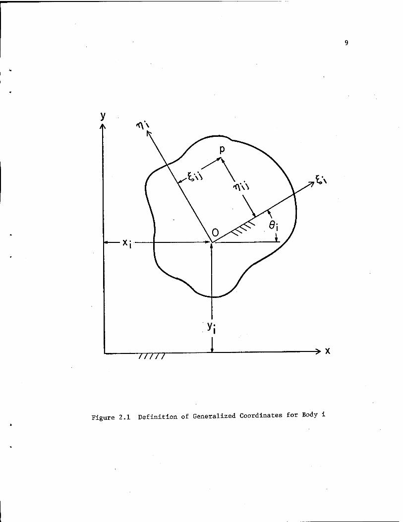
of any body or link in the system can be described by the three gener-

alized coordinates x^, y^ and Oi. These quantities can be represented

by the subvector q(i), where

(i) (2.1)

As shown in Fig. 2.1, any point p on body i of the system can be

represented by coordinates £ and ri , conveniently measured in the

local coordinate system. Knowing the generalized coordinates for the

body, it is then possible to express the position of a typical point p

in the global coordinate system.

A mechanical system generally consists of many members, connected

by joints. These joints could be looked upon as constraints imposed on

the relative motion of connected pairs of bodies. The CME formulation

thus represents joints as constraints between bodies making up the

system. These constraints are expressed as algebraic equations invol-

ving the generalized coordinates of the two connected bodies and addi-

tional geometric variables.

2.2 Position Analysis Of Mechanisms

2.2.1 Formulation of State Equation for Position

2.2.1.1 Kinematic Equations of Constraint

Consider a general system of n bodies connected by i independent

joints. Two types of joints (revolute and translation) are considered

' TT7T7 > X

Figure 2.1 Definition of Generalized Coordinates for Body i

10

in this report, each giving rise to two equations of constraint. These

equations of constraint express conditions that the motion of the two

connected bodies must satisfy to be compatible with the joint.

A system of n bodies in the plane has a total of 3n generalized

coordinates. However, if this system has £ independent joints, there

are 2£ equations of constraint between the 3n generalized coordinates.

Thus the number of free-degrees-of-freedom can be written as

m = 3n - 2£ (2.2)

where

n = number of bodies in the system

& = number of independent joints in the system

The condition m > 0 must be satisfied by all kinematic systems.

The generalized coordinates for the entire system can be denoted by the

3n position state vector z e R , where

(1)

z = (2.3)

Assuming that the system has a set of specified design variables

s b e R , the kinematic equations of constraint can be written as

$ (z,b) = 0 (2.4)

where

11

$ (z,b) =

k k d> (z,b) is the first kinematic constraint due to joint i and <j> (z,b) 2i-l 2i

is the second kinematic constraint due to joint i.

2.2.1.2 Kinematic Driving Equations

Equation 2.4 as presented in the preceding section, is a system of

2£ equations in 3n variables. Since for a kinematic system 3n > 2£, Eq.

2.4 is a system of fewer equations than unknowns. To solve for z from

Eq. 2.4, m additional equations are required. These equations can be

developed by observing that the basic purpose of designing kinematic

systems is to obtain a system that transmits motion from input links to

output links. The mechanism or machine can only be given input motion

through a set of free degrees of freedom. These free degrees of freedom

can thus be specified as functions of some free parameter, or may be

specified by some relationship between the 3n state variables. Since

all the free degrees of freedom must be specified, to drive the mechan-

ism in a unique way, m additional driving equations of constraints

arise, in the form

$ (z,b,a) = 0 (2.5)

12

where

<}> (z,b,a)

$ (z,b,a) =

<j> (z,b,a) m

P d a e R is a vector of input parameters, and <j) (z,b,a) represents the

i itn driving equation.

2.2.1.3 State Equation for Position

Combining Eqs. 2.4 and 2.5, one has 3n independent equations, which

may be written as

k $ (z,b)

$ (z,b,a) =

d $ (z,b,a)

= 0 (2.6)

Equation 2.6 is the state equation for position of the mechanism.

Specifying the design variable vector b and the input parameter vector a

makes Eq. 2.6 a system of 3n independent equations in 3n unknowns,

3n z e R . Since these equations are highly nonlinear, more than one

solution for z is possible. Conversely, for some designs and inputs,

no solution may exist.

2.2.2. Kinematic Constraint Equations

Before any technique is considered for the solution of Eq. 2.6, it

is necessary to determine the explicit form of the equations constitu-

ting this system of equations. Since kinematic equations of constraint

occur in a general form; i.e., the equations of constraint for all

13

joints of the same type have the same general form, it is sufficient to

consider a typical joint of each type. Since this report considers only

revolute and translation joints, a typical joint of each type will be

treated. Driving constraints, on the other hand, do not lend them-

selves to the same general characterization. These constraints tend

to be problem dependent.

2.2.2.1 Constraint Equations for a Revolute Joint

Figure 2.2 shows the two adjacent bodies i and j, with body-fixed

coordinate systems 0 x y and 0 x y , respectively. The origins of i i i j j j

these reference frames are located in the global reference frame by

vectors R and R , respectively. Let point p on body i be located by i j iJ

a body-fixed vector r and point p on body j be located by a body ij ji

fixed vector 7 . Points p and p are, in turn, connected by a _ ji ij Ji

vector "r . Executing a closed path from the origin of the fixed P

reference frame yields the vector relationship.

R+r + r -r - R = Ö (2.7) i ij P Ji J

Demanding that points p and p are coincident guarantees the ij ji

existence of a rotational joint between bodies i and j at this common

point. This is equivalent to the condition r = 0. Thus, Eq. 2.7 P

becomes

R+r" -7 - R = "Ö (2*8) i ij ji J

In matrix form, Eq. 2.8 can be written as

14

77777 > x

Figure 2.2 Revolute Joint

15

x

+ E(6 ) i

where

E(9) =

ij

ij

cos 6

sin 6

- E(6 ) j

ji

ji

(2.9)

-sin 6

cos 8

is a rotation matrix from the local to global reference frame.

Expanding Eq. 2.9, the equations of constraint for the revolute

joint can be written as

<b = x + E cos 9 - n sin 6 - x - K cos 6 + n _ sin 6=0 x i ij i ij i j ji J J1 3

<b = y + B, sin 6 + n cos 6 - y - K sin 6 - n cos 6=0 y i ij i ij i j ji j J1 J

(2.10)

In Eq. 2.10, x , y , 6 , x , y , and 6 are state variables. The i i i j j j

variables 5 , n , € , and n are related to the length of the ij ij ji Ji

members and hence to the design variables.

2.2.2.2 Constraint Equations for a Translational Joint

Figure 2.3 shows two bodies connected by a translational joint.

For this type of joint, the points p and p lie on a line parallel to ij ji

the path of relative motion between the two bodies. These points are

located by nonzero body-fixed vectors, 7 and r , that are perpen- ij Ji

dicular to the line of relative motion. A scalar equation of constraint

can be written by taking the dot product of "r with r . Since these ij P

two vectors are perpendicular, their dot product must vanish.

16

T7TTT ■> x

line of relative motion

between bodies

^Figure 2.3 Translation Joint

17

r • r = 0 (2.11) P ij

Using Eq. 2.7 to solve for r , Eq. 2.11 becomes P

(R + r ) - (R + r ) • r =0 (2.12) j ji i ij ij

Using the transformation matrix to express r and r in the global ji ij

reference frame, Eq. 2.12 can be written as

4 = (U - x )(U - U ) + (V - y )(V - V ) = 0 (2.13) n i i i j i i i j

where

(2.14)

U = x + %, cos 9 - n sin 6 i i ij i ij i

U = x + £ cos 9 - n sin 9 j j ji j ji j

V = y + £ sin 9 + n cos 9 i i ij i ij i

V = y + £ sin 9 + n cos 9 j j ji j ji j

Equation 2.13 restricts the motion of body i to be along a line that is

at a specified distance from and parallel to the line of relative motion.

The second scalar equation of constraint can be obtained by noting

that r and r must be parallel. This is true since both of these ij ji _

vectors are perpendicular to r . In three dimensions, this condition P

can be expressed as

r x 7 = Ö (2.15) ij ji

Expanding, the component perpendicular to the x-y plane is

$ = (U - x )(V - y ) - (V - y )(U - x ) = 0 (2.16) 9 iijj iijj

Since body i is constrained by Eq. 2.13 to move parallel to r , P

Eq. 2.16 guarantees that body j will also move along a line parallel to

r . As in the case of the revolute joint, x , y , 0 , x , y , and 6 P i i i j j j

are the state variables in the equations of constraint. Variables E, ,

n , £ , and n and related to the design variables.

2.2.3 Solution Technique for State Equations

Constraint equations for the two typical joints considered here,

Eqs. 2.10, 2.13, and 2.16, are geometrically nonlinear, due to the pres-

ence of transcendental functions of state variables. The position

state equation is thus nonlinear and a solution technique that is appli-

cable to nonlinear equations must be employed. One of the commonly used

techniques for solution of nonlinear equations is Newton's method [21].

Consider the position state equation of Eq. 2.6 for the entire

system,

$(z,b,a) = 0

Before any attempt is made to solve this nonlinear system, variables

b and a must be specified. This is reasonable, since in most iterative

design algorithms the design variable b is estimated before the synthesis

procedure is initiated. The vector of input parameters a is generally a

part of the problem specifications. The only unknowns in Eq. 2.6 are

the state variables z. Equation 2.6 is thus a system of 3n nonlinear

equations in 3n variables and a unique solution of this system will

exist locally if the stipulations of the implicit function theorem are

satisfied; ie., if the matrix

19

3$(z,b,a)

3z

3^

3z 3

(2.17)

3nx3n

is nonsingular. This condition is satisfied if the system of constraints

consists of no redundant joints.

The Newton method [21] initially requires that the state variable

z be estimated. The method then computes updates Az to this state to

obtain an improved value for the state. The improved approximation is

given by [21]

z(1+1> - ,(i) + *.<" (2.18)

where i is an iteration counter, i > 0,

Az is the solution of

Ü (zi.b.a) Az1 = - «Kz^b.oO <2-19) 3z

and the matrix [3$/3z] is called the Jacobian matrix of the system.

For large mechanisms, the system of Eq. 2.6 can be quite large,

giving rise to a large system of linear equations in Eq. 2.19. Examin-

ing the kinematic constraint equations for the two types of joints, Eqs.

2.10, 2.13 and 2.16, it can be concluded that these pairs of constraint

equations involve only the state variables of the two bodies that they

connect. These equations are thus weakly coupled and the Jacobian

matrix in the left-hand side of Eq. 2.19 is highly sparse. Efficient

sparse matrix codes [22] can thus be used for solution of Eq. 2.19.

Repeated solution of systems of equations similar to Eq. 2.19 are

required very often in the following chapters. To perform these

20

computations efficiently, the sparse matrix code initially does a

symbolic LU factorization of the coefficient matrix. Subsequent

solutions of linear systems with the same coefficient matrix, but with

different right-hand sides, can be carried out very efficiently.

Since mechanisms are being synthesized to perform over a range of

input parameters a, solution of the state equations would be required at

specific values of a. The process of obtaining the solution of the

position state equation for a specified value of a can be repeated to

obtain the solution for a desired sequence of input variables a . The

numerical efficiency of such a sequence of calculations is very good

j+l j j if a is close to a , since z(a ) serves as a good starting estimate

j+l j+l j in the computation of z(a ). If, however, a and a are not close,

then an update 6z(a ) to z(a ) is required to produce a reasonable

estimate for this computation. One such update can be obtained by

linearizing the position state equation of Eq. 2.6, keeping b fixed.

9$(z'b'aJ) 6z(aj) + 8$(z'b'a3) 6a = 0 9z 9a

or

3$<z»b»a > 6z(orK = _ 8$(z»b»a ) 6a (2.20) 9z 9a

j+l j where 6a = a - a .

j+l An improved estimate for z(a ) can thus be written as

0 J+l J j z (a ) - z(a ) + 6z(a ) (2.21)

where 6z(a ) is the solution of Eq. 2.20. Equation 2.20 has the same

coefficient matrix as Eq. 2.19, so its numerical solution is quite

efficient.

21

2.3 Velocity Analysis Of Mechanisms

Most mechanisms are driven by input sources that give input links

of the mechanism finite velocity. It is then necessary to determine

velocities of the remaining links in the mechanism, during motion of the

mechanism, over the prescribed range of inputs.

The state equation for the mechanism, Eq. 2.6, is required to hold

for all time. It can, therefore, be differentiated with respect to time

to obtain

£_ Kz.b.cO = 3«(«,b,q) * + 3$(z,b,a) ' = 0 dt dz 9^ \*-**)

The above equation can be rewritten as

[MO^M-I; z „ - 3»(z,b,cQ 0 (2<23)

3a

. 3n where z e R is the vector of generalized velocities of members of the

system.

Equation 2.23 is the velocity state equation. This equation is

linear in velocities and has the same coefficient matrix as Eq. 2.19.

As stated in section 2.2.3, this matrix is sparse and its symbolically

factorized LU form has been determined and stored. The solution of Eq.

2.23 is thus the same as solving Eq. 2.19, with a different right-hand

side. The solution of this equation is thus very efficient.

The components of the vector on the right side of Eq. 2.23 are not

so obvious. Time does not explicitly appear in the kinematic constraint

equations. However, in the driving equations, the input parameter a

could be given as an explicit function of time. The partial derivative

22

of Eq. 2.6 with respect to time can be written as

9$(z,b,a) 90

9$k(z,b)

90

9$ (z,b,a) 90"

(2.24)

k Since the kinematic constraints $ = 0 do not depend explicitly on a,

Eq. 2.24 can be rewritten as

9$(z,b,a) a „ 3a

0

9$ (z,b,a) 9a

(2.25)

where a e R is the vector of first time derivative of input parameters.

The matrix 9$ (z,b,a) in Eq. 2.25 depends on the form of the driving 9a

constraints, so it will generally be problem dependent.

2.4 Acceleration Analysis of Mechanisms

Whenever a velocity input is supplied to a mechanism, some links

experience accelerations. This is true even if the inputs to the

mechanism occur at constant velocity. Computation of accelerations is

important, since the forces experienced by links in the mechanism depend

directly on acceleration.

As noted in Section 2.3, the position state equations of Eq. 2.6

are required to hold over the entire range of inputs, so the velocity

state equation of Eq. 2.23 can be differentiated once again with respect

to time to obtain,

23

dt2 $(z,b,a) =r3^z,b,a)"|z + h ll^z.b.a) H

L 3z J |_3z L 3z J

Equation 2.26 can be written as

r"M(z,b,a)1 z = _ [3 r3$(z,b>a) Jl J L 3z J [JOY L ^ J

where

ft = J_ 3z P$(Z3a,a) "1 " + 3t(z,b,a) 8a

z I + fi = 0

(2.26)

(2.27)

a e R is the vector of second-time derivatives of input parameters

and z' e R3n is the vector of generalized accelerations.

Equation 2.27 is the acceleration state equation. This is a system

of linear equations with the same coefficient matrix as Eq. 2.19. All

the desirable properties of this coefficient matrix, as stated in

section 2.3, still hold. The solution of Eq. 2.27 is thus efficient.

The right-hand side of Eq. 2.27 involves z, which requires that the

velocity state equation of Eq. 2.23 be solved before Eq. 2.27 can be

solved. The second term in the right side of Eq. 2.27 involves

derivatives of constraints with respect to time. Differentiating Eq.

2.25 with respect to time gives

Q =

9a

0

9$ (z,b,a) . a

3a

3$ (z,b,a)

3a

(2.28)

24

CHAPTER 3

FORCE ANALYSIS OF MECHANISMS

For realistic design of mechanisms, it is necessary to impose

stress constraints on links and force constraints on joint bearings.

This requires that a force equation be derived to express internal

forces on links, in terms of the externally applied forces and system

velocities and accelerations. The applied forces could be forces due

to gravity, spring damper actuator forces, or forces from other external

sources. Two approaches are taken to arrive at the force equations. It

is also shown that these two approaches essentially lead to the same

equations for equilibrium.

3.1 Equilibrium Equation from the Principle of Virtual Work

Figure 3.1 shows a body with a body-fixed coordinate system 0 x y . i i i

An externally applied force F and an external moment T act on this ik ii

body. The point of application of force F is located by the vector

S in the body-fixed coordinate system. The virtual work of all

external forces acting on body i can be written as [23]

Ni _ _ Mi _

6w = I F • 6(R + S ) + I T «69 (3.1) i k=i ik i ik £=1 iÄ i

where

N = Total number of forces acting on body i.

25

/////

Figure 3.1 Force Acting on Body i

26

M = Total number of moments acting on body i i

Since R , S , and 0 are functions of the position state variables z, i ik i

Eq. 3.1 can be written as

_ 3R 8S \ Mi _ 39 6w -{ I F • | _Ji + _J^ SZ

+ I T • _i 6z i \k=l ik \ 8z 3z / 1=1 ±1 8z

(3.2)

The virtual work for a system of n bodies can then be written as

n 6W „ I 6W (3.3)

i=l i

Since the state equations for position of Eq. 2.6 are a system of

workless constraints, the principle of virtual work [23] requires that

6W of Eq. 3.3 be zero, for all virtual displacements that are consistent

with the constraints. These virtual displacments are all 6z

satisfying.

6$ lilöz = 0 (3.4) 3zJ

where $ = $(z,b,a). 3n

Farkas Lemma [20] now guarantees the existence of a vector y e R

of multipliers such that

T <5W - p 6$ = 0 (3.5)

3n for all 6z e R . Substituting from Eqs. 3.2, 3.3, and 3.4 into

Eq. 3.5, one has

27

n I Ni _ /9R as \ M± 3Q . T

i-1 k=l ik V-gr* -8T"/ z=1 ia -gr

(3.6)

3n which must hold for all 6z e R . Since 6z is arbitrary in Eq. 3.6,

each of its components can be varied independently, to obtain the matrix

equation

n Ni

I I f i=l k=l ik

8R 3S \ Mj_ 99 i + ik + I T . i

~9~i~ ~~5z/ Ä=l i£ -gi- G) p = 0

Equation 3.7 can be rewritten in the form

(3.7)

® -" (3.8)

where

» r?1 _ /9R as \ % ae^T

H = I < I F . i+ Ik + £ T . i i=l )k=l ik \-gi~ -gi-/ £=i iÄ -gj- (3.9)

Since the coefficient matrix of Eq. 3.8 is the transpose of the Jacobian

matrix of Eq. 2.19, this linear system is guaranteed to have a unique

solution. This Jacobian matrix, as stated in Section 2.2.3, has already

been symbolically factored and stored. Solving Eq. 3.8 is thus the same

as solving Eq. 2.19, but with a transposed coefficient matrix and a

different right-hand side. The solution of Eq. 3.8 is thus very

efficient.

28

3.2 Force Equations From Lagrange's Equations of Motion

Lagrange's equations of motion for a dynamic system can be applied

as force equations for kinematic systems. Considering Lagrange's

equations for a general constrained mechanical system [23],

r 3$ + I y _* = (Q ) + (Q )

Z=l & a7 ^ nc k c dZk

k = 1,...,3n (3.10)

where

T = kinetic energy of the system

(Q ) = nonconservative generalized force corresponding to the kth

generalized coordinate k nc

(Q ) = conservative generalized force corresponding to the kth k c

generalized coordinate

r = total number of constraints on the system, in the present

context r = 3n

p = vector of time-dependent Lagrange multipliers

In this form, Lagrange's equations are a system of 3n equations

in 3n z 's and 3n u 's. The 3n equations of constraint have also to be k i

considered along with Eq. 3.10, to solve for the 6n unknowns (3n z 's + k

3n \i 's). However, since the 3n equations of constraint have already

been solved for 3n z 's, Eq. 3.10 has only 3n u 's as unknowns. The k i

29

generalized velocities and accelerations for the system have already

been determined. Hence, the first term in Eq. 3.10 is a known quantity.

Since the kinetic energy of the system does not directly depend on the

generalized coordinates, the second term in Eq. 3.10 is zero. Equation

3.10 can thus be rewritten as

3n /a$ v

I %(_1]=(Q) +(Q>--£_/£V k=l,...,3n Ä=1 !W knc kc dt^J (3.11)

The right-hand side of Eq. 3.11 may be written as

(Q ) „ <Q ) + (Q ) _ d_ /3T \ (3.12) fc s k nc k c dt .

where

(Q ) is the total generalized forces corresponding to the gener- * s

ized coordinate z . k

Using Eq. 3.12, Eq. 3.11 can be written as

3n 9$ I W _i - (Q ) ' , k = 1 3n (3.13)

*-l Ä 3z, k s

Expressing Eq. 3.13 as a matrix equation, gives

T 8<fr\ — li = G (3.14) 3z/

G is the vector of (Q ) , k = l,...,3n k s

The force equation obtained from the Lagrange equations of

motion, Eq. 3.14, and the equilibrium equation obtained from the

where

30

principle of virtual work, Eq. 3.8, are of the same form. However, the

right side of Eq. 3.14 includes dynamic effects. These dynamic effects

include D'Alembert's forces and moments and forces and torques due to

spring dampers. For mechanisms being acted upon by static forces only,

it is possible to show that the right side of Eq. 3.8 and 3.14 are

equivalent.

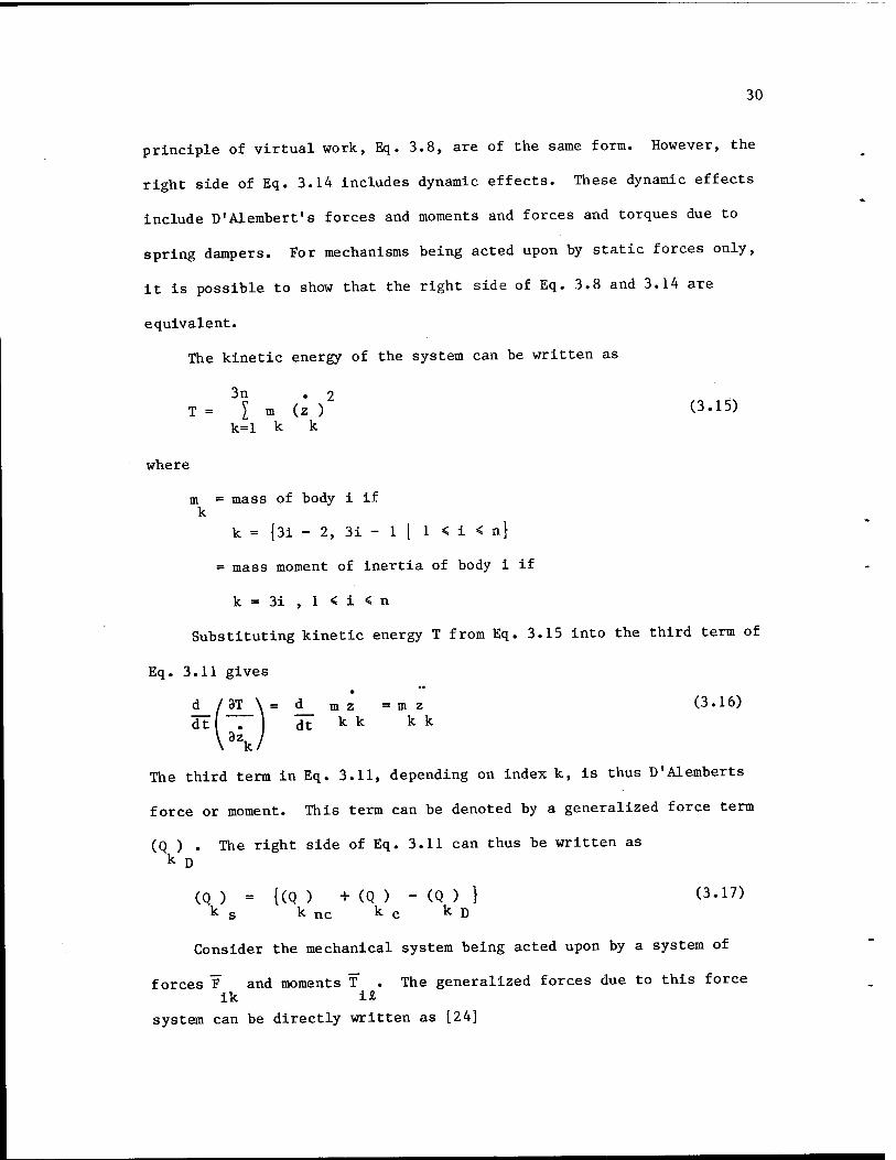
The kinetic energy of the system can be written as

3n . 9 T = I m (z ) (3.15)

k=l k k

where

m = mass of body i if k

k = {3i - 2, 3i - 1 | 1 < i < n}

= mass moment of inertia of body i if

k = 3i , 1 < i < n

Substituting kinetic energy T from Eq. 3.15 into the third term of

Eq. 3.11 gives

d_/j5T_\= d_ m z =mz (3.16) dt T~ I dt k k k k

V\) The third term in Eq. 3.11, depending on index k, is thus D'Alemberts

force or moment. This term can be denoted by a generalized force term

(Q ) . The right side of Eq. 3.11 can thus be written as k D

(Q ) - {(Q ) + (Q ) " (Q ) } (3-17> ks knc kc

kD

Consider the mechanical system being acted upon by a system of

forces ¥ and moments T~ . The generalized forces due to this force ik ±1

system can be directly written as [24]

31

n

(Q ) = I k F i=1

N± 9p Mi I F • i& + I f

£=1 i£

36

3z £=1 iÄ 3z (3.18)

where P is the vector locating the point of application of force F i£ i£

in the global reference frame.

Since the generalized coordinates being considered in Eq. 3.11 are

the same as those in Eq. 3.18, the corresponding generalized forces can

be equated; i.e.,

(Q ) = (Q ) - (Q ) k s k F k D

From Fig. 3.1, P can be denoted as i£

(3.19)

P = R + S (3.20) i£ i 11

Substituting for the right side of Eq. 3.19 from Eq. 3.18 gives

(Q ) = I k s i=l

Ni

£=1 i*

9(R+S )\ Mi 36 i i* 1 + I T . 1

£=1 I* 3z 3z -(Q ) (3.21)

k D

Writing the above equation in vector form, one has

n 6- I

i=l

Ni /3(R+S )\ Mi _ 36

£=1 iA \ 5z / £=1 it IT - (Q) (3.22)

D

By directly comparing Eqs. 3.9 and 3.22, it can be seen that the

right sides of Eqs. 3.8 and 3.14 differ by the term (Q) . Since (Q) D D

corresponds to the D'Alembert forces or moments, for static mechanisms,

Eqs. 3.8 and 3.14 are completely equivalent. For mechanisms with

dynamic effects, however, only Eq. 3.14 is valid.

32

3.3 Relating Lagrange Multipliers to Joint Reactions

The solution of Eq. 3.14 is the vector of Lagrange multipliers p.

To determine joint reactions, and the subsequent forces in the members,

it is necessary to relate these Lagrange multipliers to the joint reac-

tion forces. A method used in Ref. 13 will be used here to develop

relationships between the Lagrange multipliers and joint reaction

forces.

Consider a mechanism with n bodies and i independent joints, with

the state equations for position given by Eq. 2.6. For a typical joint

in the mechanism, the equations of constraint are

<f> = 0 r

$ = 0 r+1

(3.23)

In differential form, Eq. 3.23 can be written as

3n 3<|> «♦ = I r Sz

r i=l 3z i (3.24)

3n 3 4» 5<t> = I r+1 6z

r+1 i=l 3z i i

If this joint were to be 'broken', the equations of constraint of

Eq. 3.23 would no longer hold. However, if the defects (violations) in

constraint equations are given by Sd and 6d , respectively, then the r r+1

following conditions hold

6<f) + 6d =0 r r

(3.25) 6<|> + 6d =0

r+1 r+1

33

The displacements Sd and 6d are functions of the generalized r r+1

coordinates and can be written, s

3n 30 3n <5d = - I £_ 6z = I c 6z (3.26)

r i=l 3z i i=l i»r * i

3n 3<|> 3n 6d = - I r+1 6z = I c 6z (3.27)

r+1 i=l Ti i i=l ltr+1 i i

where

c and c are functions of the generalized coordinates. i,r i,r+l

The virtual work of the joint reactions, R and R in the direc- r r+1

tion of d and d , respectively, can be written as r r+1

<5W = R 6d + R 6d (3.28) k r r r+1 r+1

where

Joint reactions R and R can be either forces or moments, and r r+1

k is the number of the joint that has been 'broken'.

If each joint and driving constraint in the system is 'broken', the

virtual work of the reaction forces is given by

l 2Ä+m 3n 6W= I«w+ I R6d=lR6d (3.29)

R k=i k p=2£+l P P r=l r r

where p is the index of the driving constraint. Using Eq. 3.25,

Eq. 3.29 can be written as

6W = -I R H <3-30> R r=i r r

Substituting from Eq. 3.24,

3n 3n 3 A ÖW = - I I R __£. Sz (3.31) R i=l r=l r 3z i

i

34

The virtual work of the external and dynamic forces can be expressed

in the form

3n 6W = I (Q ) 5z (3.32) E i=i i S i

th where (Q ) is the generalized force associated with the i generalized

i S coordinate. Since the joints are considered broken, the equations of

constraint of Eq. 2.6 can be ignored. Hence, 6z is arbitrary and i

independent. Setting the total virtual work to zero, <5W + <5W =0, R E

for all 6z gives

3n 9,1, (Q ) = I R r , i = 1 3n (3.33)

1 s r=l r az i

In matrix form, Eq. 3.33 becomes

T 9$ 8z

R = G (3.34)

where

R = vector of reaction forces R and r

G = vector of generalized forces

Comparing Eqs. 3.34 and 3.14, it can be concluded that

R = p (3.35) i i

Thus, the Lagrange multipliers, computed as a solution of Eq. 3.14, are

the reaction forces or moments in the joints or due to the driving con-

straints. The definition of joint reaction forces R , however, depends

upon the definition of the constraint defects 8d . i

Consider now the two typical joints described in Chapter 2. The

joint reactions in the revolute joint are the forces in the global X

35

and Y direction respectively. For the translational joint, the joint

reactions are the moment in the joint and a force acting normal to the

line of translation. It still needs to be shown that the vector of

reactions R actually represents the above-mentioned reaction forces.

3.3.1 Reaction Forces in Revolute Joint

Considering a revolute joint k that connects body i and body j,

Eqs. 2.7 can be rewritten as

(r ) =(R + r - R - r \ (3.36) P k \ j ji i ij^/k

The vector r can be written in terms of its x and y components, P

r and r as

(r ) = [r r ] P k p p y

x *y K

To derive the equations of constraint for the revolute joint, the

condition r = 0 was used to get P

(r ) = P k

x ♦

= 0 (3.37)

In differential form, when <5r * 0, P

-6r x

•6r

<5<}>

6<f> (3.38)

Equation 3.38 implies that for a 'broken' revolute joint, the variation

of the x and y constraint equations represents the negative of the defect

along the X and Y axes, respectively. From Eqs. 3.24 and 3.38,

36

6d = (6r ) (3.39) Pxk

6d = (6r ) (3.40) r+1 Py k

where index r corresponds to the index of first constraint equation, due

to revolute joint k.

From Eqs. 3.39 and 3.40, it can be concluded that the Lagrange

multipliers corresponding to the two equations of constraint of a

revolute joint are the x and y reactions in the revolute joint.

3.3.2 Reaction Forces in Translational Joint

To derive the reaction forces for the translational joint, a

variation of the procedure derived in Section 3.3 is used. Since the

two equations of constraint for any joint are independent, instead of

breaking one joint at a time, only one constraint condition for the

joint is broken at a time. The unbroken constraint is thus still

valid.

Consider the second equation of constraint for the translational

joint, given by Eq. 2.15 as

((. - (U -x )(V -y ) - (V -y )(U -x ) 8 i i j j i i j j

In differential form, this is

6d> - (6U -5x )(V -y ) + (U -x )(6V -6y ) 6 i i j j i i j j

- (6V -6y )(U -x ) - (V -y )(6D -fix ) (3.41) i i j j i i j J

Substituting the differential form of U , U , V , and V from Eq. 2.14 i j i j

into Eq. 3.41 gives

37

64 = \-(K sin 6 + n cos 6 )(? sin 9 + n cos 8 ) *8 l ij i ij i ji j J1 J

-(£ cos 6 - n sin 9 )(5 cos 6 - n sin 9 )} 11 i ij i ji j Ji 3

x (69 - 69 ) (3.42) i j


64 = c (69 - 69 ) (3.43) 9 8.. i j

where c represents the term in curly brackets in Eq. 3.42. 9 ij

Thus the condition 4=0 constrains relative rotation of bodies i and j. 8

With

64 + 6d =0 6 9

as in Eq. 3.25,

6d = - c (68 - 69 ) e e.. i . j

which is proportional to a virtual relative rotation of bodies i and j.

This shows that

y 6d = -y c (69 - 68 ) 8 9 9 8. . i i

ij J

so y c is the reaction torque acting between bodies i and j, due to a 8 8.

ij

translational joint.

38

Consider now the first equation of constraint for the translational

joint, given by Eq. 2.13 as

4> = (U -x )(U -U ) + (V -y )(V -V ) n iiij iiij

In differential form, this is

fi<J> = (5U -fix )(U -U ) + (U -x )(6U -fiU ) n iiij ii ij

- (SV -6y )(V -V ) + (V -y )(6V -5V ) (3.45) iiij ii ij

Substituting the differential forms for U , V , V and V from Eq. 2.14 i j i j

into Eq. 3.45 gives

fi<(> = [-(V -y )S9 ](x -x ) + [(U -x )56 ](y -y ) n iiiij iijij

+ [(U -x )](fix -fix ) + [V -y ](5y -5y ) ii ij iiij

- (V -y )(-£ cos 0 + n sin 9 )fi0 i i ji j ji j i

- (5 cos 9 - n sin 0 )(£ sin 0 + n cos 9 )59 ij i ij i ij i ij i i

+ (U -x )(£ sin 6 + n cos 9 )69 i i ij i ij i j

- (5 sin 9 + n cos 9 )(£ cos 6 - n sin 0 )69 ij i ij i ji j ji j j

The above expression can further be simplified to

6* = [-(V -y )50 ](x -x ) + [(U -x )59 ](y -y ) n iiiij iijij

+ [U -x ](5x -fix ) + [V -y ](5y -Sy ) i i i j L i V i V

+ {(? sin 9 + n cos 0 )(£ cos 9 - n sin 0 ) ij i ij i ji j ji j

- (£ cos 9 - n sin 9 )(£ sin 0 + n cos 0 ) 1(59 -50 ) ij i ij i ij i ij i i j

(3.46)

39

Since each of the two equations of constraint for this joint are being

'broken' one at a time, the second equation of constraint for this joint,

Eq. 2.16, is valid here. From Eq. 3.43, this implies

6d> = c (69 - 60 ) = 0 (3.47)

Coefficient c has to be nonzero to get a nontrivial constraint

equation. Equation 3.27 thus implies

(66 - 66 ) = 0 (3.48) 1 j

Substituting Eq. 3.48 into Eq. 3.46 gives

6* = [-(V -y )69 ](x nc ) + [(U -x )60 ](y -y ) n'iiiij Liijij

+ [U -x ](6x -fix ) + [V -y ](6y -6y ) (3.49) i 1 i j i 1 i j

To develop an interpretation of Eq. 3.49, consider Fig. 2.3

again. Write a unit vector n along r as

1 n= {(U -x ) T+ (V -y ) J} (3.50)

|r I i i i i

Since <t> is still a valid constraint, n" is also parallel to r . The e ji

projection of the position vectors of the body-fixed coordinate systems

of bodies i and j along n can be expressed by n and n , respectively as,

n = n • R (3.51) i i

n - n • R (3.52) j j

Denote n as

n = n Y + n J (3.53) 1 2

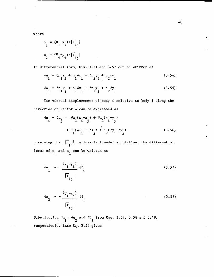
40

where

n = (U -x )/|7 | 1 i i ij

n = (V -y )/|7 | 2 i i ij

In differential form, Eqs. 3.51 and 3.52 can be written as

fin = 6n x + n fix + 6n y + n fiy (3.54) i 1 i 1 i 2 i 2 i

fin = fin x + n fix + fin y + n fiy (3.55) j 1 3 1 j 2 j 2 j

The virtual displacement of body i relative to body j along the

direction of vector n can be expressed as

6n - 6n = fin (x -x ) + fin (y -y ) i j lij 2iJ

+ n (fix - 6x ) + n (fiy -fiy ) (3.56) 1 i j 2 i j

Observing that |r I is invariant under a rotation, the differential ij

forms of n and n can be written as 1 2

(3.57) fin 1

"

(V -y ) i i 56

i

fin 2

= (U -x )

i i se i

(3.58)

Substituting fin , fin and 56 from Eqs. 3.57, 3.58 and 3.48, 1 2 i

respectively, into Eq. 3.56 gives

41

6n - Sn = 1 {[-(V -y )66 ](x -x ) i j i i i i j

r

ij

+ [(U -x )66 ](y -y ) + [U -x ](6x -6x ) iijij ii ij

+ [V -y ](6y -6y )} (3-59) i i i j

Comparing Eqs. 3.49 and 3.59 gives

6«)> = |r~ |(6n - 6n ) (3.60) n ij i j

Rewrite Eq. 3.60 as

6<|> = c (<5n - 6n ) (3.61) n n i j

ij

where c = |7 |. Thus the condition $ = 0 constraint relative n. . i-i n

translation of bodies i and j in the direction n.

With

6<() + 6d =0 n n

as in Eq. 3.25,

Sd = - c (<Sn -6n )

*±J i J

is proportional to a normal virtual relative displacement of bodies i

and j. This shows that

-y 6d = -y c (6n - <5n ) n n n n i j

so y c is the normal reaction force acting between bodies i and j,

""ij

due to a translational joint.

42

CHAPTER 4

OPTIMAL DESIGN OF MECHANISMS

4.1 Introduction

Chapters 2 and 3 provide the theory necessary to compute the

kinematics of the mechanism and the forces acting on the links of the

mechanism. It should, therefore, be possible to put design constraints

(bounds) directly on these variables or on functions of these variables.

Also, it should be possible to make extreme any of the state variables

or their functions, subject to constraints.

Most extreme algorithms used require that explicit derivatives,

with respect to design variables, of the cost and constraint functions

be provided. Computing derivatives of functions involving only design

variables is easy. However, for functions involving state variables,

the dependence on design arises indirectly, through the state equation.

Derivative computation of such functions is thus not as simple as that

for explicit functions of design variables. An adjoint variable tech-

nique that has been used for design sensitivity analysis of structural

system [20], is used in this chapter for design sensitivity analysis of

mechanisms.

4.2 Statement of the Optimal Design Problem

4.2.1 Statement of Continuous Optimization Problem

A general class of optimal design problems can be stated as:

S Find a design b R to minimize the cost function

43

ih = ip (b) (4*1) 0 0

subject to State Equations;

(A.l) Position State Equation of Eq. 2.6

$(z,b,a) = 0 (4-2)

(A.2) Velocity State Equation of Eq. 2.23

f"3$(z,b,a)~| ' _ _ 3*(z,b,a) a

L 3z J 5a

(A.3) Acceleration State Equation of Eq. 2.27

r8*(z,b,a)~| z = _ ["3 ra«(g,b,oQ Jl J _

(4.3)

(A.4) Force Equation of Eq. 3.14

3$(z,b,a) p = G (4.5) 3z

and Composite Design Constraints;

(B.l) Inequality Constraints

ip (z,z,z,u,b) < 0 , i = l,...,p (4.6) i

(B.2) Equality Constraints

lp (z,z,z,y,b) = 0 , i = p + l,...,p + q (4.7) i

Equations 4.1 to 4.7 define a general optimal design problem. Any

type of design constraint can be treated in this formulation, as long as

it can be put in a form such as Eqs. 4.6 or 4.7. The representation of

the cost function in the form of Eq. 4.1 does not restrict the technique

from being applied to cost functions involving state variables. An

upper bound technique [20] that is used in such cases is now illustrated . ••

for a general function ip (z,z,z,u,b), the maximum value of which is 0

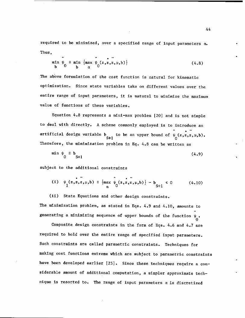
44

required to be minimized, over a specified range of input parameters a.

Thus,

min \J> = min {max ip (z,z,z,y,b)} (4.8) b ° b a °

The above formulation of the cost function is natural for kinematic

optimization. Since state variables take on different values over the

entire range of input parameters, it is natural to minimize the maximum

value of functions of these variables.

Equation 4.8 represents a mini-max problem [20] and is not simple

to deal with directly. A scheme commonly employed is to introduce an

artificial design variable b to be an upper bound of ib (z.z.z,u,b). S+l 0

Therefore, the minimization problem in Eq. 4.8 can be written as

min i|) = b (4.9) 0 S+l '

subject to the additional constraints

... . .. (i) ty (z,z,z,u,b) E {max i|> (z,z,z,y,b)} - b < 0 (4.10)

l cj U S+l

(ii) State Equations and other design constraints.

The minimization problem, as stated in Eqs. 4.9 and 4.10, amounts to

generating a minimizing sequence of upper bounds of the function \p . 0

Composite design constraints in the form of Eqs. 4.6 and 4.7 are

required to hold over the entire range of specified input parameters.

Such constraints are called parametric constraints. Techniques for

making cost functions extreme which are subject to parametric constraints

have been developed earlier [25]. Since these techniques require a con-

siderable amount of additional computation, a simpler approximate tech-

nique is resorted to. The range of input parameters a is discretized

45

into a set of grid points a , j = 1,...,T. The composite design

constraints are then required to hold at every point on this grid.

4.2.2 Statement of Discretized Optimal Design Problem

The optimal design problem, with a grid imposed on the range of the

input parameters, can be stated as follows:

s Find a design b R to minimize the cost function

♦ = * (b) (4.11) 0 0

subject to State Equations;

(A.l) Position State Equations of Eq. 2.6

$(z ,b,a ) = 0 , j = 1,...,T (4.12)

where T = number of grid points on the range of the input parameters.

(A.2) Velocity State Equation of Eq. 2.23

3$(zj,b,a;5) 9z

zi --ÜC^.b,«1) a? , J - 1.....T (4-13) 3a

(A.3) Acceleration State Equation of Eq. 2.27

9$(z3,b,aj) 3z

z = - "57

3$(zj,b,a3) ^j 3z

(A.4) Force Equation of Eq. 3.14

3$(z;3,b,a3)

'. 3z . iiJ = G3 »

Z^-fi3 » j=l,...,T

(4.14)

j = 1 T (4.15)

and Composite Design Constraints;

(B.l) Inequality Constraints

j »j "j j i|> (z ,z ,z ,u ,b) < 0, i = 1 p, j = 1,...,T (4.16) i

46

(B.2) Equality Constraints

j *j "j j ip (z ,z ,z ,p ,b) =0, i = p+l,...,p+q, j = 1 T i

(4.17)

4.3 Design Sensitivity Analysis

As noted in the introduction to this chapter, all design

optimization algorithms require that derivatives of cost and constraint

functions, with respect to design variables, be provided. Having stated

the optimal design problem, it is now possible to proceed to deriving

the derivatives of the cost and constraint functions. This derivation

is restricted to the discretized optimal design problem.

The first variation of the cost function of Eq. 4.11 can be written

simply as

8i|> (b) T ^ = ° 6b = 1° 6b (4.18)

0 3b

Since the cost function can always be reduced to a function of design

variables by the method explained in Section 4.2.1, the sensitivity of

the cost function can very simply be written in the form of Eq. 4.18.

The first variation of the composite design constraint can be

written as

+ y 5b) , i = l,...,p+q , j = l,...,x 9b

(4.19)

47

Since Eq. 4.19 is valid for equality and inequality constraints, the

index i runs from 1 to (p+q). In vector form, Eq. 4.19 can be rewritten

as

6\|> 3\|>

3z

3i|>

3z

3i|>

3z

3*±

"37" -"l

6z

6z

6z

6p

+ I ^*i I 6b 3b

i = 1, ...,p+q , j =1,...,T (4.20)

Since the state variables are functions of the design, it is

required that the variations of the state variables in Eq. 4.20 be

written in terms of variations in design. The objective is then to

write Eq. 4.20 as

T

ij ij Sip = I 6b (4.21)

ij tb

where I is the design sensitivity vector of the i constraint at the

j grid point a .

Observing that the state equations couple the design and state

variables, the first variation of the four state equations, Eqs. 4.12,

4.13, 4.14, and 4.15, can be written as

_3£] 6z + [M_\ 6b> = 0 3zj \3b. ,

(4.22)

48

3z (19 5z + 3 "ST (£)■' *+ (£) 6z'

3 "3T

3$ "35

6z - 9 IF

3$ 75

6b (4.23)

3z (£) 6z + /lil 6z + 3 (-)

6bv

3 "3T

3 "3T ¥ 6z 3

3z

_3_ 3z fe);

6z

3 "55"

3 "5z (# ; * - (£) * - (4?) 6b^ (4.24)

3z ® y 6z + 3 "5z (Ä) " *+£) ^

P)6z+G)6;+S)6:+(- 3b/

(4.25)

Moving all terms in Eqs. 4.22 through 4.25 involving 6b to the right

side, this system of equations can be written in matrix form as

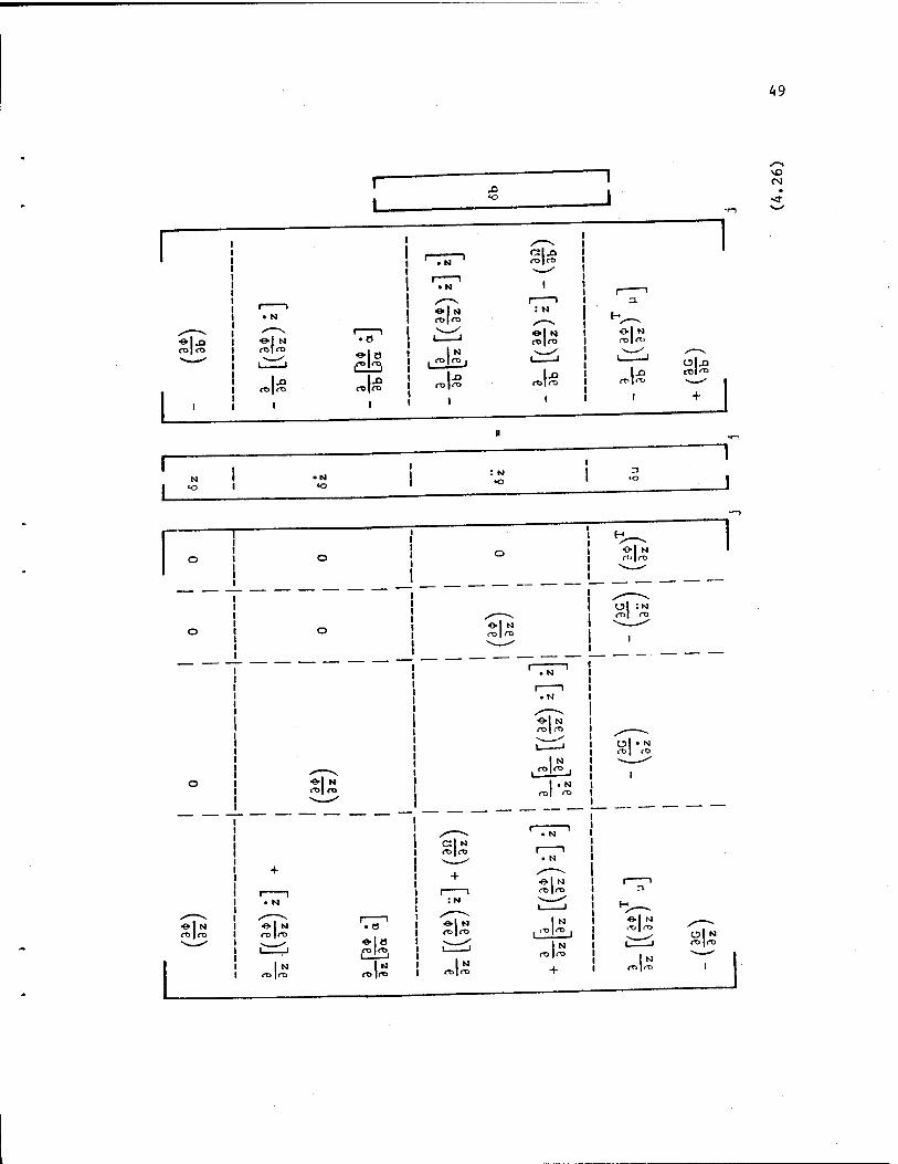
49

■»I N fO|rt>

1-°

«■18

I* rolrt>

ro|fti

1-° Olja

: N

"I

50

Equations 4.26 can be symbolically written as

j *j "j j 3 j *j "j j A(z ,z ,z ,p ,b)6U = B(z ,z ,z ,y ,b)6b (4.27)

where A represents the coefficient matrix on the left-hand side of

Eq. 4.26, B represents the coefficient matrix on the right-hand side of

Eq. 4.26, and

T

JT U

T «T "T T z z z ]1

The variation of the composite vector of state variables can be

solved from Eq. 4.27 as

6UJ = (AJ) BJ 6b (4.28)

where

A = A(z ,z ,z ,p ,b)

B =B(z ,z ,z ,y ,b)

In deducing Eq. 4.28 from Eq. 4.27, it is required that the matrix A be

invertible. The existence of such an inverse is proved in Appendix A.

Equation 4.28 expresses the variation of state variables in terms

j of variations in the design variables. Substituting 6U from Eq. 4.28

into Eq. 4.20 gives

6ip ij h%\ /3*. \ / a*.\ ht

1 1 1 1

9z • " \ 8P

L> / \3z / \3z/ \ I

j -1 j (A ) B 6b +

H. 3b

6b

(4.29)

51

j -1 To avoid calculation of (A ) , the product of the row vector of

j _1 constraint derivatives and (A ) is denoted by a composite adjoint

. .T vector A , i.e.,

•iT 3i|> i

9V 3i|> i

3ip i

3z • 3z 3z

3p uV' (4.30)

Equation 4.30 can be rewritten as

j T ij (AJ) A H. 3z

3*.

i3z

3*.

3z

(4.31)

-JJ

ij The composite adjoint vector A , as represented in Eq. 4.30, is a

12n x 1 vector. This vector can be written as a composite vector of

four (3nxl) adjoint vectors X to X Equation 4.31 can thus be 1 4

expanded as

52

CM

• N -9- : N CD

1 H I—

• N

N <D|<-O

I I

=?

■e- N rol ro

• 8

«•I O «•I N

Ol N

53

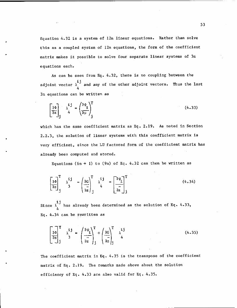
Equation 4.32 is a system of 12n linear equations. Rather than solve

this as a coupled system of 12n equations, the form of the coefficient

matrix makes it possible to solve four separate linear systems of 3n

equations each.

As can be seen from Eq. 4.32, there is no coupling between the

adjoint vector X and any of the other adjoint vectors. Thus the last

3n equations can be written as

iT

3$ 3z

ij '9^ (4.33)

J3 ' J

which has the same coefficient matrix as Eq. 2.19. As noted in Section

2.2.3, the solution of linear systems with this coefficient matrix is

very efficient, since the LU factored form of the coefficient matrix has

already been computed and stored.

Equations (6n + 1) to (9n) of Eq. 4.32 can then be written as

3$

3z

ij ij 3*.

3z

(4.34)

Since X has already been determined as the solution of Eq. 4.33, 4

Eq. 4.34 can be rewritten as

3$ "3z

ij ij (4.35)

The coefficient matrix in Eq. 4.35 is the transpose of the coefficient

matrix of Eq. 2.19. The remarks made above about the solution

efficiency of Eq. 4.33 are also valid for Eq. 4.35.

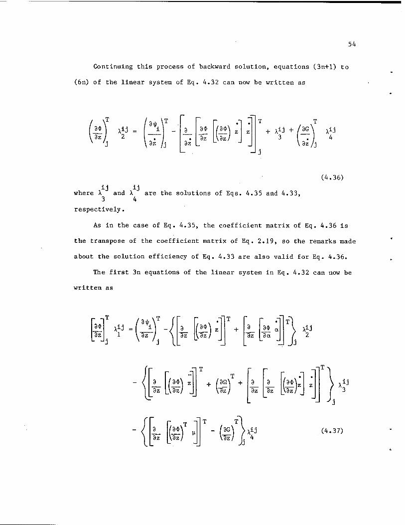
54

Continuing this process of backward solution, equations (3n+l) to

(6n) of the linear system of Eq. 4.32 can now be written as

— • • T T

_3_

3z*

9$

"9z~ p-] z

i

4

(4.36)

ij ij where X and X are the solutions of Eqs. 4.35 and 4.33,

3 4

respectively.

As in the case of Eq. 4.35, the coefficient matrix of Eq. 4.36 is

the transpose of the coefficient matrix of Eq. 2.19, so the remarks made

about the solution efficiency of Eq. 4.33 are also valid for Eq. 4.36.

The first 3n equations of the linear system in Eq. 4.32 can now be

written as

3$ 3z

T

X«. &y -/ 3 ~3T

j x 7J I (£) 3

"3¥ M a 3a

{£) :J + (£) + 3z

_3_ "37 (H); ,y

3z ®' (4.37)

55

where X , X , X are the solutions of Eqs. 4.36, 4.35 and 4.33, 2 3 4

respectively. The coefficient matrix of Eq. 4.37 is the transpose of

the coefficient matrix of Eq. 2.19, so the remarks made about the

solution efficiency of equations with this coefficient matrix are also

valid for Eq. 4.37.

Equations 4.33 and 4.35 to 4.37 are four adjoint equations associ-

ated with the four state equations. Now that the solution of the • .T

composite adjoint vector A is known, Eq. 4.30 can be substituted

into Eq. 4.29 to give

fill»1"5 - < A J BJ + I ri 1 > 6b (4.38)

Equation 4.38 expresses the variation of a composite design con-

straint in terms of the variation in design only. Comparing Eqs. 4.21

and 4.38, it can be concluded that the quantity premultiplying 6b in

th Eq. 4.38 is the design sensitivity vector of the i constraint, at the

th j grid point. Therefore,

T T /a ip £ij = Alj BJ +(i

' j

Substituting for B from Eq. 4.26, this can be explicitly written as

56

• -T 1J

T r + X _9_

8b (£) + 9 "5b 8a

J J

iJ" 9 9b

9 9b m {

*

z + 9 ~Sb~ ]*) "' +

+ IJ 9b \9z/ y - V 3b/ (4.39)

Equation 4.39 gives the design sensitivity of a composite design

constraint i at grid point j, in terms of derivatives of the position

state equation and the adjoint variables.

4.4 Design Optimization Algorithm

4.4.1 Active Set Strategy

With the design sensitivity information computed in the previous

section, one can proceed to implement the optimization algorithm of his

choice. The gradient projection algorithm with constraint error

correction [20] has been used in the past in related applications

[26, 27]. This algorithm is used here for design optimization. Before

implementing this algorithm for the present application, some observa-

tions can be made that will enhance efficiency of computation.

In connection with the composite design constraints of Eqs. 4.16

and 4.17, it can be observed that many design constraints can be put in

57

a simpler form than that indicated in these equations. Constraints that

do not involve the state variables do not explicitly or implicitly de-

pend on the input variables a. Such constraints are called 'non-

parametric* constraints. Design constraints that involve the state var-

iables are called 'parametric' constraints. It is necessary to make

this distinction, since only the parametric constraints are required to

be satisfied over the entire range of input variables a. For a given

design, the nonparametric constraints need only be evaluated once.

However, parametric constraints must be evaluated at all points on

the interval of the input variables.

An active set strategy may be adopted to determine the reduced set

ip of active constraints. Since equality constraints, parametric or

nonparametric, are always active, they are always included in the

active set \p. Nonparametric inequality constraints that are e-active

are also included in the reduced set \|>. Parametric inequality

constraints, due to their dependence on the input variable a, must be

evaluated on all points on the grid of input variable a. Some

computational efficiency can be realized from the fact that the gradient

projection algorithm, as stated in the following section, allows only

small changes in design leading to small changes in state. A design

constraint with a large violation at a given design iteration may not be

fully satisfied at the subsequent design iteration. This is so because

the algorithm used for optimization here uses only first-order

information about the design constraints. However, design constraints

are generally nonlinear. The regions of the input variable grid in

which a parametric inequality constraint is active are also not expected

58

to change rapidly from design iteration to iteration. It is thus

possible to avoid evaluating, for a few design iterations, a parametric

constraint in the region in which it is not E-active.

Design iterations in which the parametric constraint is evaluated

at each point on the a grid are defined as 'sweep' iterations.

Iterations in which the parametric constraint is evaluated only in the

active region are called 'nonsweep' iterations. The interval between

two 'sweep' iterations depends upon how rapidly the active regions are

changing. For 'nonsweep' design iterations, it is not necessary to

solve the state equations on the entire range of the input variable.

Considerable computational saving can be realized by having a large

number of 'nonsweep' iterations between successive 'sweep' iterations.

Since new active regions can only be detected during 'sweep' iterations,

having a large number of 'nonsweep' iterations separating two 'sweep'

iterations could lead to new active regions going undetected for a

number of design iterations.

Two alternative definitions could be used to define active regions

on the grid of the input variable. The first definition, as shown in

Fig. 4.1, involves determining the e-active relative maxima of the

constraint function on the a-grid. The active region is then defined to

be the set of points at which the relative maxima occur and one grid

point on either side of these grid points. The active region can thus

be defined by the index set I , R

I «{I U I 01 (4.40)

59

ö

ro ö

CVJ

ö

-£- O

r*Jr*-

0)

PS

o CO

•H to cd

pq

ß o co ß o u

•H Ö0 CJ CD -H pi H

■W

CO

c •H cd

■u co ß o

«C P4

>4-i m o o ß o

•H 4J •rl

•5* «4-1

<U P

u ß M

•rl Fn

u;

60

where

I = {j-1, j, j+1 I * > - e, i - 1,...,P, 2 < j < T-l;

\

is a relative maximum point }

I = {j. j+l * > - e, i = l,...,p, j = l;

*L


r i ij I = Id—1> j» * > - e, i = l,...,p, j = T; RR


The second definition of active region involves determining all the

points on the a grid at which the constraint function is e-active. This

set is defined to be the e-active region. Denoting this set as I , E

I - {j [ i|)1J >■- e, i = l,...,p, 1 < j < T} (4.41) E

The relative maximum strategy has been suggested for defining

active regions for parametric constraints in Ref. [25]. When applied to

constraints in mechanism optimization, this strategy many times causes

rapid oscillation of the relative maximum point on the ct-grid. A switch

to the e-active strategy overcomes this problem. As is evident from

Figs. 4.1 and 4.2, there is a penalty to be paid for this switch, since

the latter strategy requires a larger number of grid points to be

included in the e-active region.

61

ö

CD LxJ CE

UJ >

I- o <

ö

CVJ

ö

-£- O

«4-1 O

CO •H

CO nt

pq w a 4-1 o C

•rl co Cfl c n o 4-1

•H CO M c cu o tf o cu o > •H

•H M ■U 4-1 o (11

<U e Cfl

«4-1 Vi o cd

P4 ö o <1)

•H > U •H •H 4-> Ö CJ •H <U

<4-t 1 CU ö O o

H •H

CN CO • & ■* txJ

cu u 3 W

•H fn

w

62

4.4.2 Gradient Projection Algorithm

The Gradient Projection Algorithm [20] for design optimization can

now be stated in the following steps:,

0 Step U Estimate a design b , and impose a grid on the range of

the input parameters.

Step 2; Solve the state equations of Eqs. 4.12 to 4.15 for state j .j "j j

variables z , z , z , y , respectively, where j = 1,...,T if the

current iteration is a 'sweep' design iteration or j I or R

I . Note, the first design iteration must be a sweep iteration. E

Step 3: Determine the active region, depending on the strategy

chosen, and form a reduced vector f consisting of all e-active non-

parametric inequality, and all equality parametric and nonpara-

metric constraints. For inequality parametric constraints, the

constraints evaluated in the active regions are included in i|>.

ij ij ij ij Step 4: Compute adjoint variables X , X , X ' and X from Eqs.

4 3 2 1

4.33, 4.35, 4.36 and 4.37, respectively, and construct design

ij sensitivity vectors £ of Eq. 4.39 for the constraint functions in

Ij ij i\). Form the matrix A=[i ], whose columns are the vectors Z

~T corresponding to constraint functions in ty. Thus, Sty = A 6b

W0 M Step _5: Compute the vector M and matrix M from the following

relations;

~T -1 0 M - A W £ (4.42)

*+0 0

where % is defined in Eq. 4.18 ~T _! -

M = A W A (4.43)

63

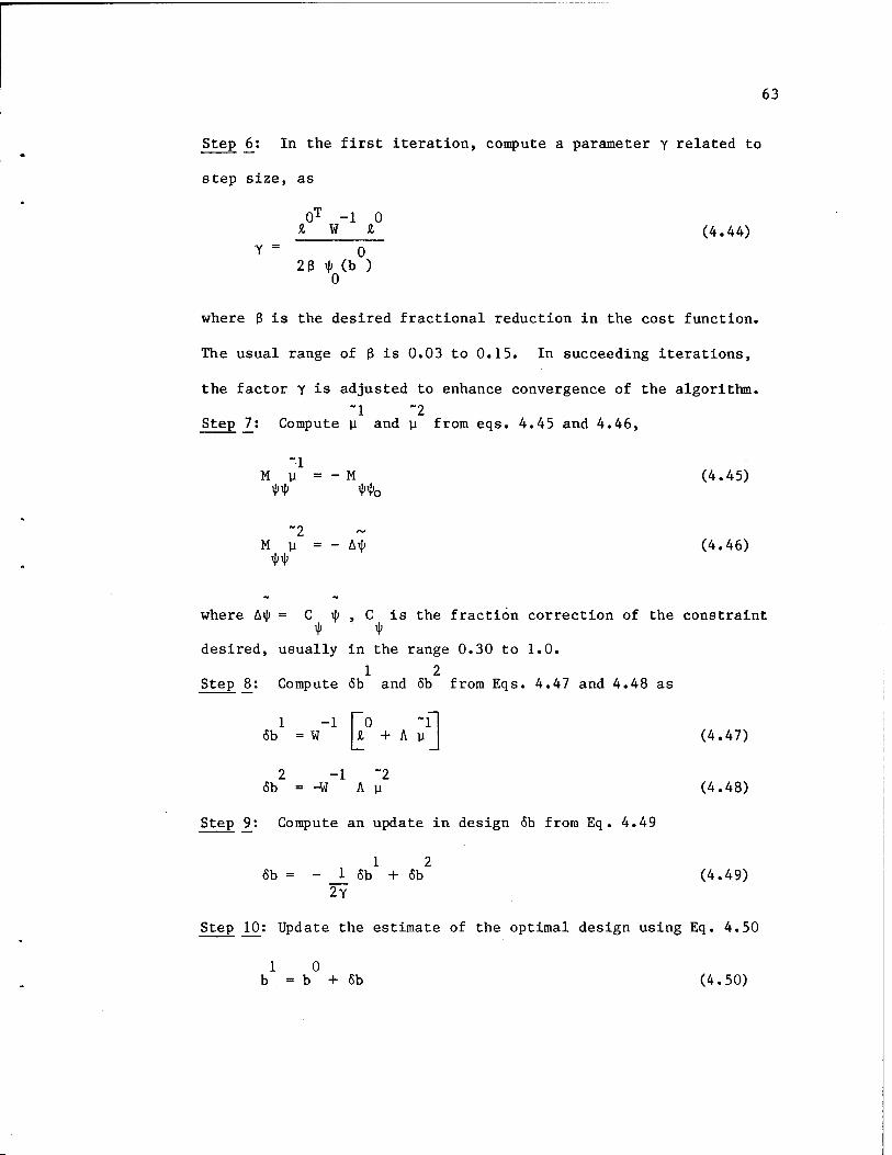
Step _6: In the first iteration, compute a parameter y related to

step size, as

: -1 0 (4.44)

0T -1 0 I W I

Y = 0 23 if» (b )

0

where $ is the desired fractional reduction in the cost function.

The usual range of ß is 0.03 to 0.15. In succeeding iterations,

the factor y is adjusted to enhance convergence of the algorithm.

"1 ~2 Step 7: Compute y and y from eqs. 4.45 and 4.46,

(4.45) "1

M y = - M Mo

"2 M y = - Aif» (4.46)

where Lty = C if» , C is the fraction correction of the constraint if; if)

desired, usually in the range 0.30 to 1.0. 1 2

Step 8; Compute 6b and 6b from Eqs. 4.47 and 4.48 as

1 -1 To -fl 6b = W h + A y J (4.47)

2 -1 "2 6b = -W Ay (4.48)

Step 9: Compute an update in design 6b from Eq. 4.49

1 2 6b = - J_ 6b + 6b (4.49)

2Y

Step 10: Update the estimate of the optimal design using Eq. 4.50

1 0 b = b + 6b (4.50)

64

Step 11: If all constraints are satisfied to within the prescribed

tolerance and

6b S 1 ' I W (6b )

i=l i i

1/2

< 6 (4.51)

terminate the process. Where 6 is a specified convergence

tolerance. If Eq. 4.51 is not satisfied, return to Step 2.

65

CHAPTER 5

NUMERICAL EXAMPLES

5.1 Example 1 - Kinematic Synthesis of a Path Generator

5.1.1 Problem Description

A segment of a straight line is required to be generated by a point

P on the coupler of the four-bar mechanism shown in Fig. 5.1. In

addition to having the lengths of various links as design variables

(b to b ), the orientation of the base link, body 1, is a design

variable (b ). The orientation of the reference line with respect to

the base link, about which the input variable a is measured, is also a

design variable (b ). The other two design variables (b and b ) are as 4 7 8

indicated in Fig. 5.1. The length of the base link is kept fixed at 10

units. This problem is the same as Example 3 in Ref. 26.

5.1.2 Problem Formulation

The motion specification for this problem requires that the devi-

ation of the y coordinate of coupler point P from zero in the global

coordinate system be minimized. The position vector for point P, in

terms of design and state variables, can be written as

b2 R = x3 + cos 6 ( 2 + b7 cos bo) ~ b7sin bgsin 8 I

b2 = y3 + sin 63( £ + b7 cos bg) + b7cos 9 sin bg J (5.1)

L

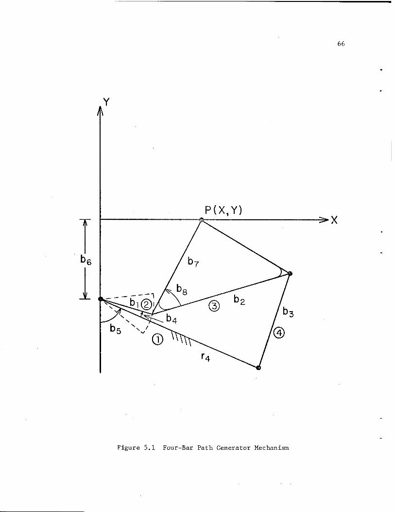
66

T

JL ,^--r--

^X

Figure 5.1 Four-Bar Path Generator Mechanism

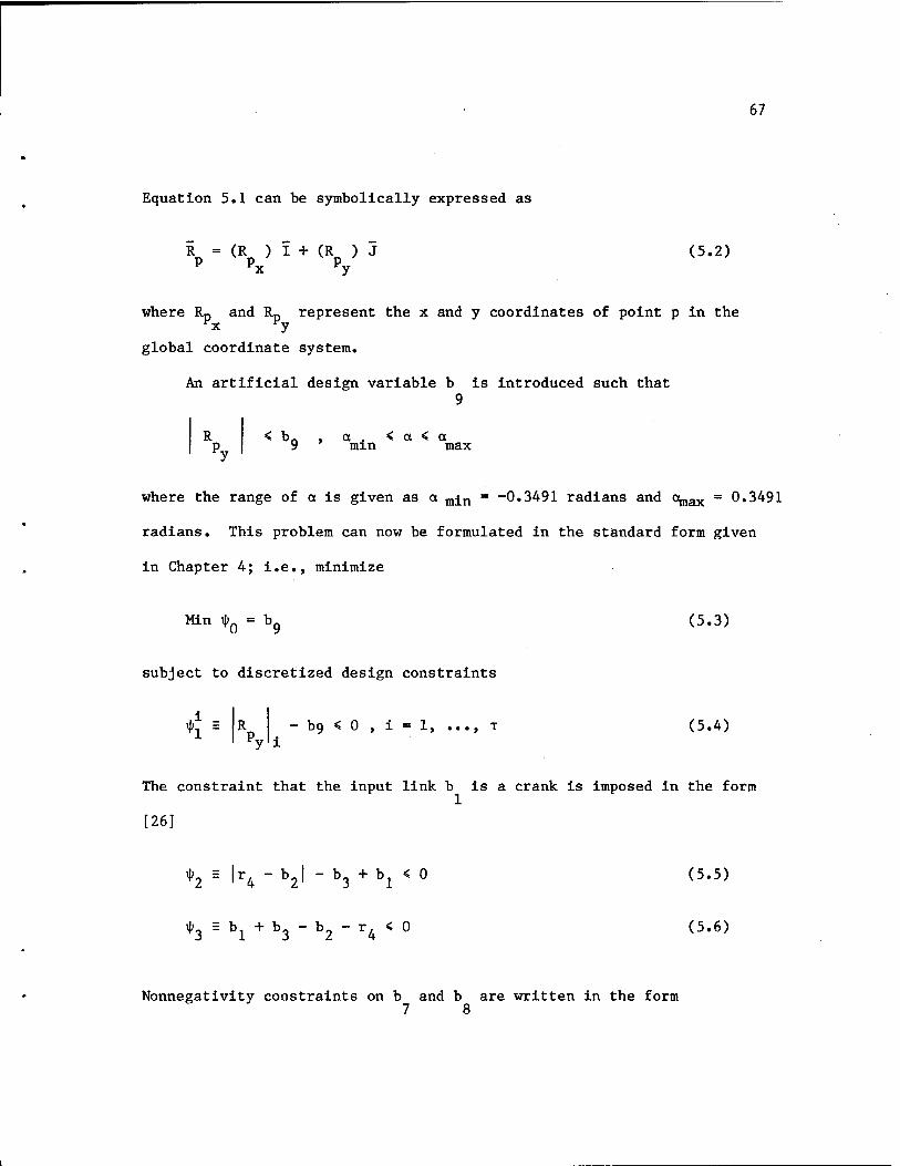
67

Equation 5.1 can be symbolically expressed as

R = (R ) I + (R ) J P P P

(5.2)

where Rp and Rp represent the x and y coordinates of point p in the Fx Hy global coordinate system.

An artificial design variable b is introduced such that 9

< bn , a. < a < a 9 min max

where the range of a is given as a ^n = -0.3491 radians and o^ax = 0.3491

radians. This problem can now be formulated in the standard form given

in Chapter 4; i.e., minimize

Mn ^0 = b9 (5.3)

subject to discretized design constraints

- bg < 0 , i = 1, ..., T (5.4)

The constraint that the input link b is a crank is imposed in the form

[26]

*2H lr4-b2l "b3+bl <0

*3 =- bl + b3 - b2 " r4 < °

(5.5)

(5.6)

Nonnegativity constraints on b and b are written in the form 7 8

68

\ = "b7 < 0 (5.7)

% E-b8 < 0 (5.8)

The error bound constraint in Eq. 5.4 is imposed over a grid of

T = 19 equally spaced points on the range of a. The driving kinematic

constraint for this problem is given as

*1 E 62 " {b5 + b4 + al} = ° » i = 1,...,19

5.1.3 Numerical Results

5.1.3.1 Verification of Design Sensitivity Analysis

It is necessary to numerically verify that the technique developed

in Chapter 4 has been correctly coded. The procedure used is briefly

explained here.

The problem is set up through user supplied routines and input

data. The code is allowed to run for 2 design iterations. On the basis

of the design sensitivity vector calculated and the change in design 6b

obtained in the first iteration, changes in the constraint can be pre-

dicted. This predicted value can be compared with the actual change

obtained when the constraint functions are evaluated in the second de-

sign iteration. If the design sensitivity analysis is valid, the pre-

dicted and actual changes in constraints should agree within a reason-

able tolerance. This procedure is now used to verify the design sensi-

tivity analysis for this problem. Consider grid point 19, where the

parametric constraint of Eq. 5.4 is violated during a design iteration.

69

T A1»19 = [-0.67893, -.04693, 0.06083, 2.30624, 2.85158, -1.0,

0.99853, 0.34923, -l.o]

T r The change in design at this iteration is 6b = [0.01663, 0.00115,

-0.00149, -0.05650, -0.06985, 0.02450, -0.02446, -0.00853, -0.2096].

The predicted change in the constraint is thus given as

T 1 19 1 19

Aip1'1* = lL'iy 6b = -0.1832 P

The actual change in the constraint function is evaluated as

1 19 A*7» = -0.1709 A

The difference between the predicted and actual change is 6.7%. The

design sensitivity analysis is thus considered to be valid.

5.1.3.2 Optimization Results

The results obtained from the optimization procedure are as

presented in Table 5.1. None of the nonparametric constraints was

active at the optimum. As given in Table 5.1, there are 5 critical

points on the grid of the input parameter at the optimum design, where

the error in function generation is a relative maximum. The maximum

error obtained in Ref. 26 for this problem was about 0.0019, which is

greater than that obtained by the present technique.

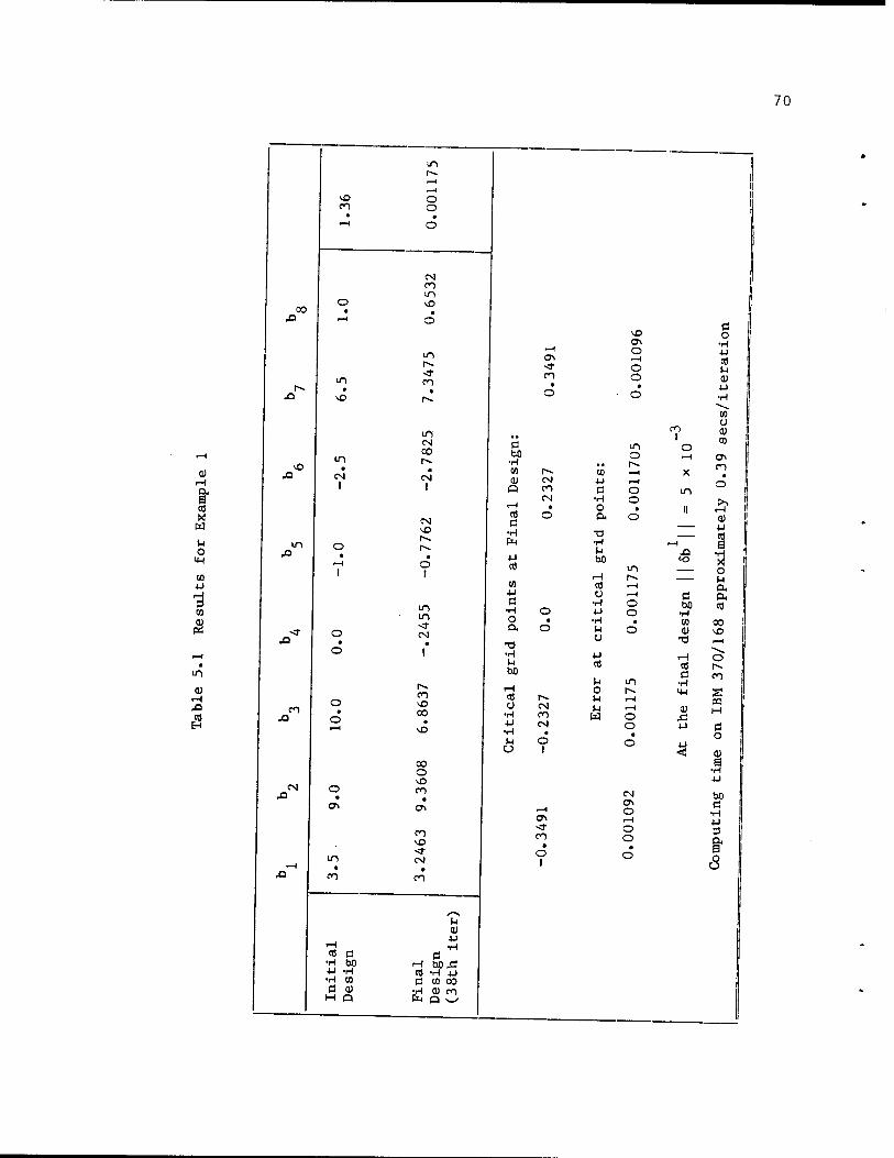
70

CO

00

CO X w u o

<4-l

CO 4J r-f 3 CO

ä

t-i 43

CM I

O

I

o o

o o

o

co

en

O O

CM CO m

CO

m CM 00

• CM

I

CM

• o

I

m CM

I-» CO vO 00 •

00 O vD CO

CO ^O -* CM • CO

vO <y>

1—4 o <3\ ~^ <r o CO o

bO •H CO 1^« (1) CM P CO

CM H •

CO O a •H 1*

4-1 ct)

CO 4-1 a

•H o O • ft o

T3 •H t-l DO

rH cfl 1-^ o CM

•H CO 4-> CM •H • H O U 1

CO I

CO 4J a

•H O ft

•v •H

00

cfl O

•H u O

4-1 cd

n o u u w

CO

o I

o

o o

O o

o o

CM <Tv O i-H o o

X

II

43

C 00

•H CO eu

CO ß

CU ,ß 4-1

3

cfl ß •H DO H 4J -H Cfl •i-l CO ß ß CU •H M Q P*

<u 4-1 •H

ß b0,ß

•H 4J CO 00 CU CO p ^

ß O

cfl M <U 4J •H

CO CJ cu !! CO

CF\ CO

eu 4J cfl S

•H

O

P. ft cfl

CO

O

co

2 M M

a o CU s

00 ß

•H 4J 3

&

71

5.2 Example 2: Kinematic Synthesis of a Rigid Body Guidance Mechanism


The mechanism shown in Fig. 5.2 is to guide the book-carriage of a

library book-stacking vehicle [28]. It is required that point P

describe a path given in Table 5.2. In addition it is required that

body 8, the carrier, assume angular orientation at specific input grid

points, given in Table 5.2. The mechanism is driven by the rotating

crank, which is body 4.

Design variables b , b , and b radially locate the 3 joints of the 12 3

ternary base link. The angular orientation of these radial lines is

specified by the three angles 3 =73.5°, 3 = 61.5°, and 3 = 71.5°. 12 3

Design variables b to b are the lengths of links 4 to 9, respectively. 4 9

The length of link 10 is taken as 10 units. Other angles specified in

Fig. 5.2 are given as 3 = -50.0°, 3 = -63.0°, and 3 = -103.0871°. 4 5 6


The global x and y coordinates of the coupler point P can be

written in terms of design and state variables as

b8 R = {x0 + cos Q0(r7r- ~ A cos 3, ) - A sin 60 sin 3, } I p o o A 4 OH

b8 + {yg + sin QgC^- - A cos ^) + A cos 6g sin 34} J (5.9)

Equation 5.9 can be symbolically written as

R = (R ) I + (R ) J (5.10) P P P x y

72

ß\ ßzß* s> X

Figure 5.2 Rigid-Body Guidance Problem

Table 5.2 Output Specifications for Example 2

73

Grid pt 6.(deg) 4

(P ) cms x d

(P ) cms y d

(6g)d(deg)

1 -62.5 11.943 6.458 103.0871

2 -40.5 12.712 6.288 107.9571

3 23.0 13.214 6.075 111.2971

4 0.0 14.553 5.774 114.2471

5 31.0 15.824 5.716 113.5876

6 50.5 16.396 5.71 110.3871

7 78.5 16.388 6.465 103.0871

74

where Rp and Rp represent the x and y components of the position x y

vector of point P.

An artificial design variable b is now introduced to impose the 10

following constraints:

(Rp } -(px>dl <Clb10 ' j =1' *•" ?

(R ) - (P ), p yd y

c„b,' , i =1. .... 7 2 10

<Vg-<Vd <c3b1Q , j = 1, ..., 7

where (p ) and (p ) are the desired x and y coordinates of point p, x d yd

(9 ) is the desired orientation of link 8 and (6 ) is the generated 8 d 8 g

orientation of link 8.

In standard form, this problem is formulated as; minimize

*0 5 bio (5.11)

subject to discretized design constraints

4 -=

4

(R ) - (Px)d , " Cjb < 0 , j = 1, ..., 7 (5.12) Px 'J

(R ) - (p ), p y d

(98>g - <88>d

j - c2b1Q < 0 , j = 1, ..., 7 (5.13)

i " c3b10 < ° » j = l> '"' 7 (5-14)

The driving kinematic constraint for this problem is given as:

±d _ Qd i n n +1 = 61 ~ "l " ° » i = 1, .... 7

75



The procedure outlined in Section 5.1.3.1 is used here to verify

the design sensitivity analysis. The design sensitivity vectors at a

certain iteration for the three error constraints were obtained as

T A1»1 = [-0.44247, -0.05346, 0.77940, 0.44687, 0.01196, -0.06584,

0.16044, -0.18837, -1.19525, -1.0 ]

T £2'4 = [-1.42060, 0.03326, 0.32397, -0.13204, 0.48655,

-0.46958, 0.60349, 0.14956, -0.65320, -l.OJ

T Ä3»6 = [0.24504, -0.15474, -0.08915, 0.51890, -0.82560, 0.20605,

-0.23002, -0.49248, 0.88695, -1.0 ]

The change in design obtained at this iteration was

6bT = [-0.00368, 0.02838, -.001735, 0.002504, 0.01337, 0.02730,

0.00148, -.00806, 0.003155, -0.002811 ]

The predicted changes in the constraints can thus be computed as,

T Ail»1'1 -A1»1 5b = -0.00096

P

T Ai|£»4 = £2'4 5b = -0.00060

T Ai^'6 = Ä3,6 SI = -0.000014

The actual changes in these constraint functions were

A*1»1 = (0.003869 - 0.004834) = -0.000965 A

A/'4 = (0.0023898 - 0.002992) = -0.000604

A

AiJ3,6 = (0.00006938 - 0.00008909) = -0.0000197

76

Comparison of the actual and predicted changes in the constraints

shows that for the first two constraints there is a good agreement.

However, for the third constraint the agreement is not as good. This

can be attributed to numerical error in differencing very small numbers


The results from the optimization procedure are presented in Table

5.3. The first parametric constraint was active at 3 critical points,

the second at 2 critical points, and the third at only one critical

point. The maximum error obtained using the present technique is 20%

higher than that reported in Ref. 28.

5.3 Example 3 — Two degree of Freedom Function Generator


The relationship u = (1 + v)log (1 + w) is to be mechanized in 10

the region 0 < v < 1, and 0 < w < 1. This problem is similar to the

numerical example given in Ref. 6. The mechanism to be used for

function generation is a seven-link mechanism shown in Fig. 5.3. The

inputs v and w are the displacements of bodies 5 and 6, respectively.

These displacements are measured from reference positions, measured

along the global axis, which are taken as design variables b and b . 1 2

The output u of the mechanism, is the displacement of body 2 relative

to the origin of the global coordinate system. This displacement is

measured along the line of translation that makes an angle y = 27.881°

with respect to the global x-axis. the lengths of links 3, 4, 6 and 7

are design variables b to b . The angle between links 4 and 6 is 4 7

77

u c^ • o o CM

1«! U r^ O cfl U • • s w

m •

o

CN vO

a\ m • X

m •

in

oo vO

m • 00

m CN o • o

00 vO • ,0 vO

r^ m CT\ o CM 0 CM

CM r^ m o o o • o> • • • • r* -* • o o 1—1 o

-Q co m l

CO

! w

o

CO 4J

3 CO

CO

m cj H ^3

m

o

m

CM CM ^o CM

\0

00

1-^

—1

-3- CXi <t

O CO ■ •

CO CM ■—I

O -•

CO rH

<t CM m i—< •

CM o

o • m

o r-l

oo m

CO •

^^ I-I co 4J

i-i 1-1 ctf C c

•H bO i-i M J3 4-1 •W CO •rl 4-1 •rl CO ö w m c 0) •H CD sf H Q pt< Q ^

m CM

I

o

•rl I-I DO

CO CJ

CM o

CM

Cd CM .—i e • •rl m

CO • 4J cr c w •rl

O M a. o

M-l •o •H

CO I-I 4-1 M

cfl cj

•r-l

I-I CJ

4J CO

u o u u w

o o • CO CM I

w i-J o

«-I

4J c

•H O

cfl CJ

•r-l 4-J •rl I-i U

CM o

o m

o m

CM I

x

CO

m —I CM O II

CO

er w C r-l

CO 4-1 c •rl O

(0 cj

•H 4J •H

U

H O I-I u w

Cd

I-i O

4-1

CO 4J c •rl O

cfl cj

•rl 4J •H H o

Cd

C •H

CO 4-1 C

■rl O

CO cj

•rl 4-) •1-1 U CJ

4J cfl

I-i o M I-I

Cd

£

(3 DO •rl CO a>

Cfl Ö

CJ je

Ü

ö o

•H 4J Cfl M a> 4-1 H

CO o <u

co m

<D 4J cfl a

•H

O I-i P. o. cd

oo

o

CO

g

(3 o

I 4-1

DO Ö •rl 4J 3

a- o u

78

u o •u nl u 0) c 0) o a o

•H 4-1 o Ö s

a o 0) a)

i

o I

0) 0)

M 01 O

CO

m 0)

3 00

•H

79

design variable b . The other parameters related to this problem are 3

as indicated in the Fig. 5.3.


The displacement of the output slider, body 2, along the line of

translation can be written in terms of the generalized coordinates of

body 2, as

X2 U =-s- (5.15)

cos 3,

where 3 =27.881°. 1

An artificial design variable b is introduced such that 8

u - u, I. , < b„ j = 1, ..., 4 g d |j,k 8 J ' '

where (u ). represents the generated value of u, for specific values

i k of the input parameters oc and ou, and (u,). , is the desired value of

i k u, for the same values of the input parameters cc and a . The

function to be generated in this example,

(Vj,K= (1 + 4> 1Og10(1 + °£>

This problem can be formulated in standard form as; minimize

*0Hb8 (5-16)

Subject to discretized design constraints

*lf J' ^ 5](Vj.k-(1 + 0?> 1Ogl0(1 + ^ | "b8 <0'

j,k = 1,...,4 (5.17)

80

The error bound constraint is imposed on a grid of four equally spaced

points, Fig. 5.4, on each of the input variables a and a . Thus a 1 2

total of 16 grid points are obtained. No other design constraints are

imposed in this problem. The driving kinematic constraints for this

problem are given as

(frj = x5 - (bx + or[) = 0 , j = 1,...,4

d k <f>2 = xg - (b2 + <x2) = 0 , k = 1 4



The design sensitivity of the upper bound constraint, Eq. 5.17, at

iteration no. 11 and grid point j = 1, k = 4 was obtained as

T A1»1»4 = [0.15546, 0.23616, -0.57531, -1.45199, 1.29105, 0.06958,

-0.32795, -1.0]

The change 6b in design was

6bT = [-0.01027, 0.00197, 0.01753, 0.00938, 0.01017, 0.01178,

-0.00640, -0.00070]

The predicted change in constraint is thus computed as

T A*1»1»4 = £1»1»4 6b = -0.00805

P

The actual change in constraint was obtained as

A^'1'4 = 0.07259 - 0.08055 = -0.00796

81

w f

1.0 4,1 4,2 4,3

4,4

3,1 3,2 3,3 3,4

2,1 2,2 2,3 2,4

1,1 1,2 1,3 M_ 0.0 1.0 V

Figure 5.4 Grid Spacing for Problem 3

82

The difference between the actual and predicted change in the con-

straint is 1.0%, which verifies that the design sensitivity analysis

for upper bound constraint of Eq. 5.17 is valid.


The results of the optimization procedure for this problem are as

presented in Table 5.4. The maximum error in function generation

obtained from the present procedure is about 25% higher than that

obtained in Ref. 6. This can be attributed to 2 differences in the

formulation. First, the design variables used in the present problem

and Ref. 6 are not the same. Second, the grid points in the present

formulation and Ref. 6 are not identical. Location of grid points is

known to have a very significant effect on the error in function

generation [14].

5.4 Example 4 - Stress Constrained Design of a Four-Bar Mechanism


The four-bar mechanism shown in Fig. 5.5 has its input crank

rotating at a constant angular velocity of 300 rpm. This mechanism is

to be designed for minimum mass, requiring that bending stresses in

mobile links 2, 3, and 4 do not exceed an allowable stress. The design

variables in the mechanism are the circular cross-sectional areas of

the three mobile links. The link lengths are kept fixed at the values

specified in Table 5.5. The mass density and allowable stress in the

links are as given in Table 5.5. Specifications for this problem are

the same as those of example 1 in Ref. 30 and example 1 in Ref. 29.

83

CO

I«! m u o

M-l

CO 4J iH

in

Cd H

u o u vO u LO O w o • O • X o o 1

o> ö o

-* m •H r-~ • -H 4J

ja eg • CM M

<U 4-1 H

co in oo -* Ü

vO • vß 1 0) ,£> 1—4 •

■—I

CM m

o

X

I-t

Cfl

o •

oo ^ II i-l m • i—t <U

,o o • —— 4J ^ s

•H X o M

CM A r-~ •^f Ö &

<r • o\ M CO ,fi o m •H

o CO

rH

00

—1

o CM CO f- o> vO Ö en

en r^. -tf •H ja • • •4-4 a

CM 1

CM 1

4-1

4-j

H

(3 O

-3- m <! <D CM • <r s

.o CM • CM

•H 4J

DO Ö

O oo ■rl m en 4-1 r* m 3

H • • & JQ o o s

5 s-\ U <u 4-1

iH •H n) C c

•H t>0 H MJS 4-> -H CO iH 4J •H (0 ß (00 C 0) •H a> en

fa O ^ H Q

84

Jnt. 3

Jnt. 4

Figure 5.5 Minimum Weight Design of Four-Bar Mechanism

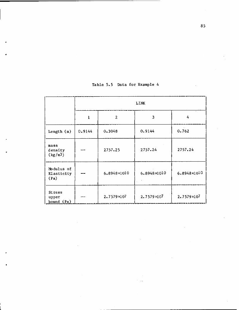
Table 5.5 Data for Example 4

85

LINK

1 2 3 4

Length (m) 0.9144 0.3048 0.9144 0.762

mass density (kg/m3)

— 2757.25 2757.24 2757.24

Madulus of Elasticity (Pa)

— 6.8948x1010 6.8948x1010 6.8948x1010

Stress upper bound (Pa)

— 2.7579x107 2.7579x107 2.7579x107

86


As shown in Chapter 3, the Lagrange multipliers obtained as a

solution of the force equation are directly related to reaction forces

in the joints. As shown in Fig. 5.6, reactions at the ends of a link

could thus be represented by the appropriate Lagrange multipliers.

However, to compute bending moments, the end reactions are required to

be expressed in a local coordinate system. As shown in Fig. 5.6, the

y , p system of forces at a joint must be transformed to the P , k k+1 k

P system. k+1

The external load on the beam depends upon the normal acceler-

ation. To compute the distribution of normal acceleration along the

length of the link, a cross section of the link at distance v along the

x axis is considered. The position vector for point c can be written

as

Rc = x± I + y. J + v(cos 6. I + sin 8 J) (5.18) i

where x , y and 0 are the three generalized coordinates locating the

body in the plane and I and J are unit vectors in the global X and Y

directions.

The absolute acceleration of point c can thus be written as

R = (x. - v cos 6. 6" - v sin 0 6)1+ c l x i i V

•2 (y. - V sin 6_, 0^ + v cos 0.8.) J

i i i xi

Transforming the global unit vectors to the local system,

acceleration normal to the length of the link can be written as

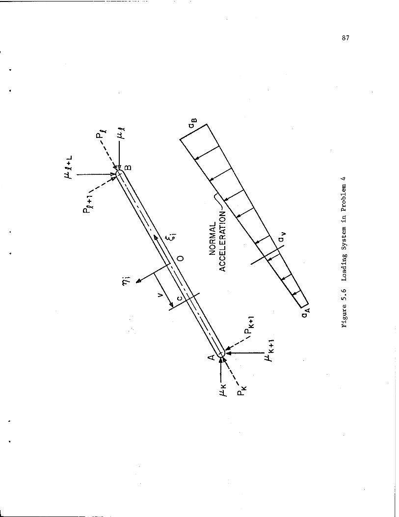
87

+

C \ cT

O u

c •H

§ J-l CO >■> en 60

•5 *d

ca o

\D

0)

a 60

88

a = (- x. sin 6. + y. cos 6.) + v 6. (5.19) y. l l l l l '

where x., y. and 6. are the generalized accelerations of body i. From

Eq. 5.19, it can be seen that the normal acceleration varies linearly

along the length of the link.

The distributed loading on the beam can thus be written as

f. = -m„ {(-x. sin 6. + y. cos 8.) + v 8.} (5.20)

where m is mass per unit length of link i. Ä l


f± = -m£ aÄ + v 6. (5.21) i i

where a, = -x. sin 6. + y. cos 6.. X.. 1 1 Jx x l

Since elementary beam theory is used to compute bending stresses,

it is necessary to first determine the point of maximum bending moment.

This is the point at which the shear force changes sign. The shear

force at any point D, at a distance X from 0, can be written as 0

Fs = Pk+l+ -**. /°. (a* + V V dV

l -Äi/2 i

= pk+i " m*. [aÄ.(xo + -T) + -T ^xo " -T^j (5'22)

At the point of zero shear force, the right-hand side of Eq. 5.22

will be zero, giving rise to the condition

89

e. 9 aÄn/i A

2 9. P^,

■TXS + -*1X0+C-T---VL-^-0 (5.23)

Solving for X from Eq. 5.23. 0

-a„ ± /a2 - 26. x * x k+1

"*i V *i 1 2 8 ^ X„ = = i (5.24)

The maximum bending moment can thus be written as

*i X0 M0. = Pk+1^T+ Xo) +ml I K. + v 6iKn- X0) dv (5.25)

Integration of Eq. 5.25 gives

X^ Ä3 XnÄ2 "I

+ 6i I--|+ ^ + Al]j Ö.26)

where X is given by Eq. 5.24. 0

Equation 5.26 is valid only for links 3 and 4. The crank, link 2,

is rotating at constant angular velocity and has no normal

acceleration. The maximum moment on this link is the torque required A

to drive the mechanism. It occurs at r\ = - -i- and is given as

\ = yi2 (5.27)

Since the links are of circular cross section, the area moments of

inertia can be written in terms of the design variables as

90

>2i

where 2 < i < 4 is the link number. The distance of the extreme fiber

from the neutral axis is given as

* - ,b- 1 T IT

The absolute values of the maximum bending stresses, from

elementary beam theory [31], can now be written as

(O,. =4 * b'i v3/2 Vl

M0 » 2 < i < 4 (5.29)

where MQ is given by Eq. 5.27 for i = 2 and by Eq. 5.26 for i = 3 and 4

The optimization problem can be written in standard form as;

minimize

*0 ~ P2 \ bl + p3 S b2 + P4 \ b3 (5.30)

where p_ is mass density of link i, subject to discretized design

constraints

«£> b'k+1 (5.31)

a 1 < K < 3

where o^ is allowable stress and T is the total number of grid points.

For this problem 19 grid points were considered. The driving

constraint for this problem is given as

+1 = e2 - ai = 0 . j = 1, — ,19

91



The design sensitivities of the stress constraints at a certain

iteration were obtained as

T A1»17 = [-1801.18, 1928.83, 853.239]1

T Ä2»15 = [ 0.0 ,-3481.67, 0.0 ]T

T Ä3'15 = [ 0.0 , 0.0 ,+2051.6 ]T

The change in design at this iteration was

6bT = [2.022X10-5, 1.76xl0~5, -8.626xl0~6]

The predicted changes in the constraints can thus be computed as

T AI|L,'

17 = £1,1? 6b - -0.00983

T AIJL'

15 = Ä2'15 6b = -0.0613

T Ai||'15 = Jt3'15 6b - -0.01739

The actual changes in the constraint function were obtined as

A*A'

17 = -0'0097

Aip2,15 = -0.06002

A^3'15 = -0.0169

Comparison of the actual and predicted changes shows that the two

sets of data agree to within 2.5%. The design sensitivity analysis can

thus be considered valid.

92


Results of the optimization procedure are presented in Table 5.6.

Results obtained in Refs. 29 and 30 for this problem are also given.

As can be seen, there is a substantial difference between the designs

obtained. This difference is attributed to the fact that Refs. 29 and

30 use different methods for stress analysis than used in the present

formulation. The constraint functions are, therefore, not identical.

5.5 Example 5 - Dynamic Balancing of a Four-Bar Mechanism


It is desirable to make the shaking forces of a mechanism vanish

by balancing the mechanism. However, doing so introduces additional

difficulties. For example, the RMS bearing forces could increase by

as much as 100 percent [4]. In the present example, the four-bar

mechanism shown in Fig. 5.7 is considered. A trade-off is resorted to,

in which the RMS shaking forces are minimized, while limiting increase

in the ground-bearing forces. Minimization of RMS shaking force is

accomplished by modifying the inertial properties of the output, link

by adding a circular counterweight to it, as shown in Fig. 5.8. The

mass and location of this counterweight are design variables.

Data for the mechanism considered in this problem are given in

Table 5.7. This problem is the same as the single counterweight

optimization example given in Ref. 4.

Table 5.6 Results for Example 4

93

Design Variables

Mass (kg)

bx(m2) b2(m2) b3(m2)

Starting Design

1x10-1 1x10-1 1x10-1 546.26

Optimal Design 30th iter

1.03x10-3 0.621x10-3 0.1169x10-3 2.686

Results from Reference 29

0.401x10-3 0.385x10-3 0.385x10-3 2.134

Results from Reference 30

0.953x10-3 0.488x10-3 0.309x10-3 2.703

1 -6 At the final design | |5b | | = 2.5 x 10

Approximate CPU time (IBM 370/168) = 1.25 Sec/Iteration

94

Jnt. 2

%

Jnt. 3

Jnt. 1

Figure 5.7 Four-Bar Mechanism to be Dynamically Balanced

95

Jnt. 3

Jnt. 4

COUNTER

WEIGHT

MASS=b!

Figue 5.8 Schematic of Counterweight Used in Dynamic Balancing

Table 5.7 Data for Example 5

96

LINK

1 2 3 4

Length, (m) 7.62x10-2 2.54x10-2 1.016x10-1 7.62x10-2

Mass (kg) — 4.588x10-2 1.084x10-1 6.602x10-2

Moment of inertia @ C.G kg-m2

— — 3.208x10-4 6.779x10-5

97


The RMS shaking force for the four-bar mechanism being considered

here is given as [4]

(FM/G)RMS = V"b SV t(F14X + F34x)2 + ^14Y + F34Y^d92

(5.32)

where F and F are the ground-bearing forces at joint 1, in the X 14X 14Y

and Y directions, respectively; F and F are the ground-bearing 34X 34Y

forces at joint 4, in the X and Y directions, respectively; and 9 is 2

the angular orientation of the input crank.

The RMS ground-bearing forces are given as [4],

(F41X + F41Y^d9? (5'33) RMS i -■■

= Jl_ r27r r''"2 ■ -2

"V 2TT J0

RMS

where [F J and (F ) are the RMS ground-bearing forces at joints 1 RMS 4 RMS

1 and 4, respectively.

There is a one to one correspondence between the design variables

used here and those used in Ref. 4. Location of the center of mass of

the combined link, in terms of design variables and given data, can be

written, using relationships given in Ref. 4, as

„0 1 ( 0 0 •> c4 = P4-Tir— Kp4-bib

2) <5-35>

and

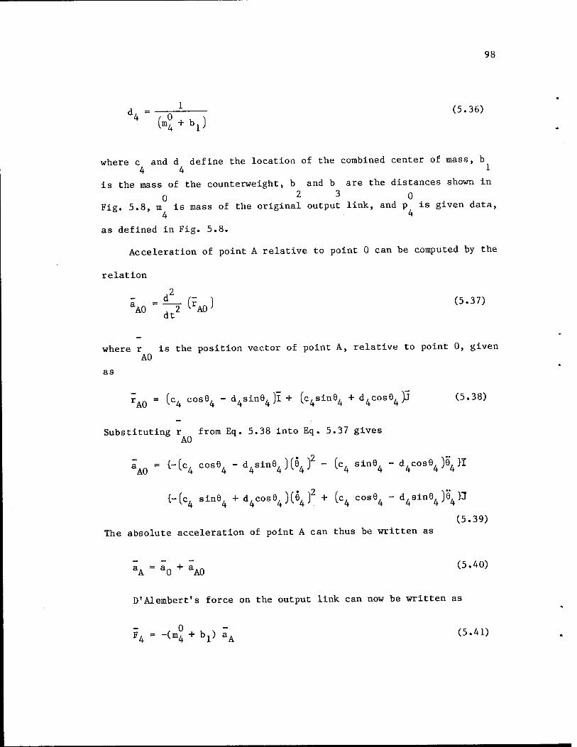
98

d, -—yr-i (5.36) 4 (m°4 + bl)

where c and d define the location of the combined center of mass, b 4 4 l

is the mass of the counterweight, b and b are the distances shown in

0 2 3 o Fig. 5.8, m is mass of the original output link, and p is given data,

4 4

as defined in Fig. 5.8.

Acceleration of point A relative to point 0 can be computed by the

relation

aA0 .2 l A0J at

where r is the position vector of point A, relative to point 0, given A0

as

rAQ = (c4 cos64 - d4sin94)l + (c4sine4 + d^osejj (5.38)

Substituting r from Eq. 5.38 into Eq. 5.37 gives A0

= {-(c. cos6, - d.sine. )(6 f - (c. sin9 - d COBB )5 }I aA0 = 1_lC4 CUöO4 " U4ÖJ"UU4 J^ü4 J ~ ^4 """4 "4V'V""'4 J~k

{-(c4 sme4 + d4cose4)(e4)2 + (c4 cose4 - d4sine4)e4

(5.39) The absolute acceleration of point A can thus be written as

I = ä + ä (5.40) aA a0 aA0

D'Alembert's force on the output link can now be written as

F4 - -(m° + bx) a"A (5.41)

99

Computation of D'Alembert moments requires the combined moment of

inertia of the original link and the counterweight. Since the

counterweight is circular, it's moment of inertia about point B is

given as

I* = b^b^ + b^/2 (5.42)

Using the parallel axis theorem [23], the combined moment of inertia of

the original link and the counterweight can be written as

where I is the combined moment of inertia about point A and 1 is the A 0

moment of inertia of the original link about point 0. Since moment of

inertia of the original link given in Ref. 4 is about point C, the

parallel axis theorem must be used to write I in Eq. 5.43 in terms 0

of the given data,

Ic = I0 + m° (p°)2 (5.44)

Substituting for I in Eq. 5.42 from Eq. 5.44 gives 0

0 0 2 0 2 2 *A = IC " m4(p4} + m4(c4 + V

+ I* + b1 [(pj - c4 + b2)2 + (b3 - d4)2] (5.45)

The D'Alemberts moment can now be written as

M = - IA 64 (5.46)

100

Forces in the ground bearings, used in Eqs. 5.32 to 5.34, can be

related, from the results of Section 3.3.1, to the Lagrange multipliers

by the following relationships

F = -u 14X ^4

F = -U 14Y 5

(5.47)

F = y 34X 10

F = P 34Y 11

Equations 5.32 to 5.34 can thus be rewritten as

(FM/GVS ^ 2 IT ' ^4i ^*K--4 + "10)2 + (""5 + "ll)2J d62 (5-43)

V4i /*["2o+"2i]de2 (5-50) (VRMS

The optimization problem can now be stated in the standard form

of minimizing

ib = (F , ) (5.51) V0 v M/GyRMS

subject to constraints

/ ,1VW _ x <0 (5.52) Fl

# E^VRMS _ ! <0 (5.53)

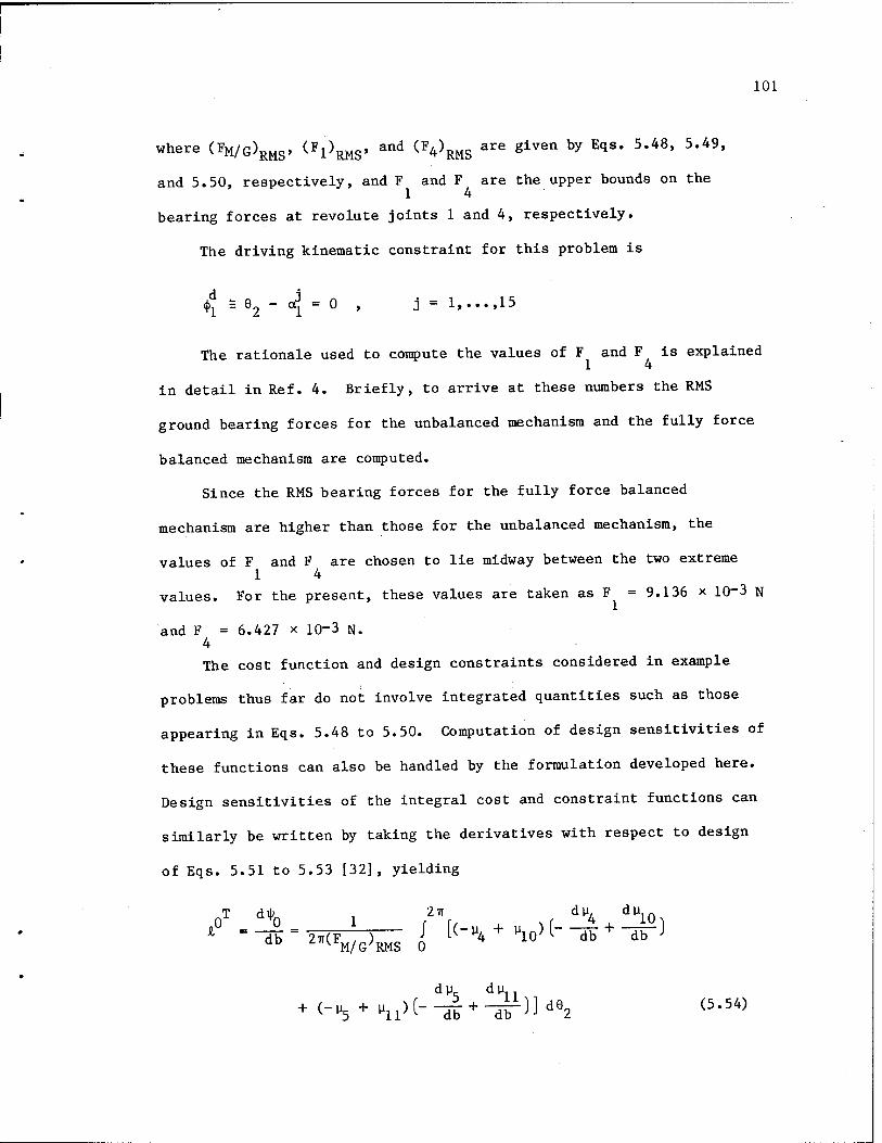
101

where (FM/G)RMS> (FARMS' &nd (F4}RMS are giV6n by EqS* 5*48' 5*49'

and 5.50, respectively, and F and F are the upper bounds on the 1 4

bearing forces at revolute joints 1 and 4, respectively.

The driving kinematic constraint for this problem is

4>j £ e2 - dj - 0 , j - 1, ...,15

The rationale used to compute the values of F and F is explained 1 4

in detail in Ref. 4. Briefly, to arrive at these numbers the RMS

ground bearing forces for the unbalanced mechanism and the fully force

balanced mechanism are computed.

Since the RMS bearing forces for the fully force balanced

mechanism are higher than those for the unbalanced mechanism, the

values of F and F are chosen to lie midway between the two extreme 1 4

values. For the present, these values are taken as F = 9.136 x 10~3 N

and F = 6.427 x 10-3 N. 4 The cost function and design constraints considered in example

problems thus far do not involve integrated quantities such as those

appearing in Eqs. 5.48 to 5.50. Computation of design sensitivities of

these functions can also be handled by the formulation developed here.

Design sensitivities of the integral cost and constraint functions can

similarly be written by taking the derivatives with respect to design

of Eqs. 5.51 to 5.53 [32], yielding

T di|> , 2TT du, du n

QD ^'M/G'RMS o

dp d y

102

,T ,1 \ , 2TT dy. du

Numerical integration of Eqs. 5.54 to 5.56 requires evaluation

of the integrand at specific points in the interval of integration.

Computation of the derivatives of Lagrange1s multipliers appearing in

the integrands of Eqs. 5.54 to 5.56 can be routinely done in the

present formulation. The computer code is forced to treat u , u , u 4 5 10

and u as constraint functions, purely for the purpose of computing

the design sensitivity. The design sensitivity of these functions is

evaluated at points on the 6 grid corresponding to the nodes of the

15 point Gauss-Legendre integration formula [33]. Since constraints 1 2

i|> and ty do not depend on the input parameter, they are nonparametric

constraints.



The design sensitivity vectors of the cost and constraint

functions, at a certain design iteration, were obtained as

T Ä0 = [-.000799, .02880, .004828]

1T

r = [4.1542, -12.7106, 3.1470]

?T

r = [3.9492, -14.846, -.3122]

103

The change in design in this iteration was

6b = [-0.000885, 0.001334, 0.000373]

The predicted change in cost is thus computed as

T Ai|i0 = 9? 6b = 0.0000409

P

Predicted changes in constraints are computed as

A^1 = -.01946 P

Ai|>2 = -.0234 P

The actual changes in the cost and constraints were

Ai|£ = 0.000057

Ai|£ = -.011355

A^ = -.01406

Comparing the predicted and actual changes in cost and constraint

functions, it can be seen that the two sets of data no not agree well.

This can be attributed to the highly nonlinear nature of the cost and

constraint functions. This can be seen by computing the predicted

change in constraint, using an average design sensitivity vector. For

example, consider constraint 1, for which the design sensitivity vector

averaged over the two design iterations is

,T [* LTT, - [4.1145, -12.4848, 3.1727] L JAVE L

The predicted change in the constraint, on the basis of the averaged

design sensitivity vector, is

104

Kw= --°1183

As can be seen, this figure agrees closely with the actual change in

the constraint.

5.5^3.2 Optimization Results

Results obtained from the optimization procedure are presented

in Table 5.8. For the purpose of comparison, the design variables used

in Ref. 4 are converted to those used in the present formulation. The

ratio of the RMS shaking force for the partially balanced mechanism to

that for the unbalanced mechanism is given by r . As can be seen from

Table 5.8, a substantial reduction in RMS shaking force is obtained by

using the present formulation. Results obtained from the present

formulation and those in Ref. 4 differ substantially. This difference

is attributed to the fact that the present formulation imposes the RMS

ground bearing force constraints as inequality constraints and Ref. 4

considers these to be equality constraints. Significant improvement in

design from the present formulation over that from Ref. 4 is thus to be

expected and is evident from Table 5.8.

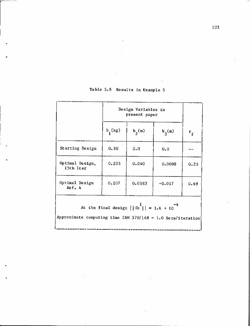
Table 5.8 Results in Example 5

105

Design Variables in present paper

r f

b (kg) 1

b (m) 2

1 b3(m)

Starting Design 0.30 0.0 0.0 —

Optimal Design, 15th Iter

0.203 0.040 0.0098 0.25

Optimal Design Ref. 4

0.207 0.0183 -0.017 0.69

1 -4 At the final design ||6b || = 1.6 x 10

Approximate computing time IBM 370/168 = 1.0 Sees/iteration

106

CHAPTER 6

CONCLUSIONS AND RECOMMENDATIONS FOR FURTHER RESEARCH

6.1 Conclusions

The five examples presented in Chapter 5 were studied to evaluate

versatility and effectiveness of the technique developed in the

previous chapters. In light of the results obtained with these

examples, the following conclusions may be drawn:

1. The constrained multi-element technique developed in

Chapters 2 and 3 for modeling kinematic systems is general

enough to represent a wide variety of planar mechanisms.

2. The adjoint variable technique has been successfully applied

for design sensitivity analaysis of planar mechanisms,

considering both kinematic and force response of mechanisms.

3. Due to the generality of the constrained multi-element

technique for modeling and the adjoint variable technique for

design sensitivity analysis, the synthesis and design

technique developed in this research is very general and

versatile. This is evident from the variety of examples

given in Chapter 5.

6.2 Recommendations for Further Research

In the preceding section it was pointed out that the state space

technique developed in this research has demonstrated its potential

107

as a versatile and powerful tool for kinematic synthesis and design.

However, to fully realize this potential, it is recommended that the

following areas be further investigated:

1. The gradient projection algorithm stated in Chapter 5 was

used as the optimization algorithm in this research. This

algorithm, in its present form, is insensitive to

nonlinearity of the state equations and in the cost and

constraint functions encountered in kinematic synthesis and

design problems. In addition to its insensitivity to

nonlinearities, this optimization algorithm often produces

designs for which the mechanism locks up in some position.

This is primarily due to the algorithm's not having any

information about the kinematics of the mechanism.

It is thus desirable to investigate alternate optimization

algorithms that have the following desirable characteristics:

(i) The algorithm should be sensitive to nonlinearities

arising in mechanism synthesis and design problems,

(ii) The algorithm should produce design changes that are

compatible with kinematic requirements of the mechanism.

2. The gradient projection algorithm, like many other opti-

mization algorithms, does not guarantee a globally optimal

design. To be assured that the optimal design produced by the

optimization technique is globally optimal, it is necessary to

start the procedure with different initial designs. In most

mechanism synthesis problems a substantial effort has to be

108

put into producing acceptable initial designs. It is thus

desirable to investigate techniques that guarantee conver-

gence to globally optimal designs.

3. The computer code used to implement the theory developed

in the previous chapters was of an experimental nature. Some

of the areas in which this code could be refined are as

follows:

(i) Significant improvements should be made in the solution

procedure for state equations,

(ii) Computation of derivatives of user-supplied driving

kinematic equations and cost and constraint functions

should be carried out with a symbolic manipulation

language.

(iii) Implementation of the code for execution in a

conversational mode would be highly desirable.

4. Synthesis and design of three-dimensional mechanisms is

currently at an elementary level. The theory developed here

for synthesis and design of planar mechanisms is extendable to

three-dimensional mechanisms and should be pursued.

109

REFERENCES

1. Freudenstein, F., "Structural Error Analysis in Plane Kinematic Synthesis," ASME, Journal of Engineering for Industry, Ser. B, Vol. 81, No. 1, Feb. 1959, pp. 15-22.

2. Kramer, S.N. and Sandor, G.N., "Selective Precision Synthesis - A General Method of Optimization for Planar Mechanisms," ASME, Journal of Engineering for Industry, Ser. B, Vol. 97, No. 2, 1975.

3. Tepper, F.R. and Lowen, G.G. , "General Theorems Concerning Full Force Balancing of Planar Linkages by Internal Mass Redistribution, ASME, Journal of Engineering for Industry, Ser. B, Vol. 94, No. 3, Aug. 1972, pp. 789-796.

4. Tepper, F.R. and Lowen, G.G., "Shaking Force Optimization of Four-Bar Linkage with Adjustable Constraints on Ground Bearing Forces," ASME, Journal of Engineering for Industry, Ser. B, Vol. 97, No. 2, May 1975, pp. 643-651.

5. Berkof, R.S., "Force Balancing of a Six-Bar Linkage," Proceedings of the Fifth World Congress on the Theory of Machines and Mechanisms, July 8-13, 1979, Montreal, Canada, pp. 1082-1085.

6. Ramaiyan, G. and Lakshminarayan, K. , "Synthesis of Seven Link Two- Freedom Linkage with Sliding Inputs and Outputs using Identical Link Positions," Mechanisms and Machine Theory, Vol. 11, No. 3, 1976, pp. 181-185.

7. Ramaiyan, G., Lakshminarayan, K. and Narayanamurthi, R.G. , "Nine- Link Plane Mechanisms for Two-Variable Function Generation - II. Synthesis," Mechanisms and Machine Theory, Vol. 11, No. 3, 1976, pp. 193-199.

8. Mariante, W. and Willmert, K.D. , "Optimal Design of a Complex Planar Mechanism," ASME, Journal of Engineering for Industry, Ser. B, Vo. 99, No. 3, Aug. 1977, pp. 539-546.

9. Thronton, W.A., Willmert, K.D. , and Khan, M.R., "Mechanism Optimi- zation via Optimality Criterion Techniques," Journal of Mechanical Design, Trans. ASME, Vol. 101, No. 1, July 1979, pp. 392-397.

10. Rubel, A.J. and Kaufman, R.E., 'KINSYN III: A New Human Engineered System for Interactive Computer Aided Design of Planar Linkages," ASME, Journal of Engineering for Industry, Vol. 99, No. 2, March 1977, pp. 440-455.

110

11. Rucci, R. J. "SPACEBAR: Kinematic Design by Computer Graphics," Computer Aided Design, Vol. 8, No. 4, October 1976, pp. 219-226.

12. Erdman, A.G. and Gustavson, J.E. "LINCAGES: Linkage Interactive Computer Analysis and Graphically Enhanced Synthesis Package," ASME paper 7 7-DET-5.

13. Paul, B., "Analytical Dynamics of Mechanisms - A Computer Related Overview," Mechanism and Machine Theory, Vol. 10, No. 4, 1975, pp. 481-507.

14. Hartenberg, R.S. and Denavit, J., Kinematic Synthesis of Linkages," McGraw-Hill Book Co., 1964.

15. Sheth, P.N. and Uicker, J.J. , 'IMP Integrated Mechanism Program], A Computer Aided Design System for Mechanisms and Linkages," Journal of Engineering for Industry, Trans. ASME, Vol. 93, No. 4, 1971.

16. Paul, B., Kinematics and Dynamics of Planar Machinery, Prentice-Hall, 1979.

17. Orlandea N., Chace, M.A. and Calahan, D.A., "A Sparsity-Oriented Approach to the Dynamic Analysis and Design of Mechanical Systems," Part I and II, ASME, Journal of Engineering for Industry, Ser. B., Vol. 99, No. 3, 1977.

18. Wehage, R.A. and Haug, E.J., "Generalized Coordinate Partitioning for Dimension Reduction in Analysis of Constrained Dynamic Systems," ASME paper no. 80-DET-106. To be published in Journal of Mechanical Design.

19. Haug, E.J. , Wehage, R. and Barman, N.C., "Design Sensitivity Analysis of Planar Mechanism and Machine Dynamics," ASME, Journal of Mechanical Design, Vol. 103, No. 3, pp. 560-570, 1981.

20. Haug, E.J. and Arora, J.S., Applied Optimal Design, John Wiley & Sons, 1979.

21. Atkinson, K.E., An Introduction to Numerical Analysis, John Wiley & Sons, 1978.

22. United Kindgom Atomic Energy Authority: "Harwell Subroutine Library: A Catalogue of Subroutines," Report AERE R7477, Subroutine Librarian, CSS Division, Atomic Energy Research Establishment, Harwell Didcot, Oxfordshire, England 0X11 ORA, 1973.

23. Greenwood, D.T., Principles of Dynamics, Prentice-Hall, 1965.

Ill

24. Goldstein, H., Classical Mechanics, 2nd ed. , Addison-Wesley Publishing Company, 1980.

25. Kwak, B.M., Parametric Optimal Design, Ph.D. Thesis, University of Iowa, Iowa, City, 1975.

26. Kwak, B.M. and Haug, E.J. "Optimal Synthesis of Planar Mechanisms by Parametric Design Techniques," Engineering Optimization, 1976, Vol. 2, pp. 55-63.

27. Sohoni, V. and Haug, E.J., "A State Space Method for Kinematic Synthesis of Mechanisms and Machines, ASME paper No. 80-DET-43. To be published J. of Mechanical Design, ASME, 1981.

28. Bhatia, D.H. and Baccl, C, "Optimal Synthesis of Multiloop Planar Mechanisms for the Generation of Paths and Rigid Body Positions by the Linear Partition of Design Equations," ASME paper No. 74-DET-14.

29. Khan, M.R., Thornton, W.A. and Willmert, K.D., "Optimality Criterion Techniques Applied to Mechanical Design," Journal of Mechanical Design, ASME, Vol. 100, April 1978, pp. 319-321.

30. Imam, I. and Sandor, G.N., "A General Method of Kineto-Elastodynamic Design of High Speed Mechanisms," Mechanicisms and Machine Theory, Vol. 8, 1973, pp. 497-516.

31. Ugural, A.C. and Fenster, S.K. , Advanced Strength and Applied Elasticity, American Elsevier Publishing Company, 1975.

32. Taylor, A.E. and Mann, W.R., Advanced Calculus, Wiley, 1972.

33. Carnahan, B., Luther, H.A. and James, W.O., Applied Numerical Methods, John Wiley & Sons, 1969.

112

APPENDIX A

PROOF OF NONSINGULARITY OF MATRIX A IN EQUATION 4.27

Matrix A defined in Eq. 4.27 is the coefficient matrix on the

left-hand side of Eq. 4.26. A proof of the existance of an inverse for

this matrix will now be developed. The Jacobian matrix (9$/3z) that j

occupies a band along the diagonal of matrix A is assumed to be

nonsingular. This assumption is initially made in Section 2.2.3 and is

still valid here.

Consider Eq. 4.22, with perturbation in design 6b = 0,

9$ 9z

6z =0 (A.l)

Since the coefficient matrix of Eq. A.l is nonsingular, by theorem 7.2

of Ref. 21, Eq. A.l implies that

6zJ = 0

Consider Eq. 4.23 with 6b = 0,

(A.2)

9$ "9z

6z = -J9 9z

U_ z 9z 9z

9$ a 9a

6z (A.3)

Substituting for 6z from Eq. A.2, Eq. A.3 becomes

9$

"9z~ 6zJ = 0 (A.4)

By the same argument, Eq. A.4 implies

6zJ = 0

Consider Eq. 4.24 with 6b = 0 and Eqs. A.2 and A.5,

[s| 6z = 0

As deduced previously, Eq. A.6 implies

••J 6z = 0

Consider Eq. 4.25 with 6b = 0 and Eqs. A.2, A.5 and A.7,

T -i 9$ 8z

6u = 0

113

(A.5)

(A.6)

(A.7)

(A.8)

The coefficient matrix of Eq. A.8 is the transpose of the Jacobian

matrix of Eq. A.l. Since the Jacobian is nonsingular, its transpose

also has the same property. Eq. A.8 thus implies

6u = 0 (A.9)

From the definition of the composite state variable vector U given

in Section 4.3,

6U 6z 6z "T

6z 6u (A.10)

-J

Substituting from Eqs. A.2, A.5, A.7 and A.9, Eq. A.10 can be written

as

6 U = 0

Now consider Eq. 4.27 with 6b = 0,

J J - A 6 U = 0

(A.ll)

(A.12)

114

As shown in the above, Eq. A.12 implies that Eq. A.11 holds, i.e.,

j 6 U = 0

By theorem, 7.2 of Ref. 21, this is equivalent to the statement that

(A ) is nonsingular.

115

APPENDIX B

DERIVATIVES OF KINEMATIC CONSTRAINT EQUATIONS

B.l Notation

Before any derivatives of Kinematic Constraint Equations are

calculated, the following notation is introduced for a revolute joint§

R = £ cos 8 - n sin 8 lj ij

R = £ sin 8 + n cos 8 2 ij i lj 1

R = E, cos 8 - n sin 8 3 ji j ji J

R = £ sin 9 - n cos 8 4 ji j ji J

(B.l)

9R 9?. . 9n RBI = - Ü cos 6, - H. sin 6.,

9b ab 1 3b 1 k k k

RB2 = 8R

2 9b k k

sin 8 - i

1J cos 8 9b i k

3R 95 . 3n

3b k

= Ji "ST"

k

cos 8 - j

- J1 sin 6 3b ~ j k

RB3 =

9R 9£. 3n.. RB4 = 4 = Ü sin 8 + ii cos 8,

"3F" ~5E k k

■3F^ k

(B.2)

116

35 . 3n.. 35.. 3n.. The partial derivatives ij., _ ^j., Jji and _ J_, will take on

"5F~~ "3F" 1F"~ k k k

IF

nonzero values only if design variable b is related to the lengths of k

body i or j.

Similarly for translational joint, the following notation is

introduced:

Tl = £ cos 9 - n sin 0 ij ■ i ij i

T2 = 5 sin 9 + n cos 9 ij i ij i

T3 = £ cos 9 - n sin 6 ji j Ji J

T4 = K sin 6 + n cos 9 ji j J1 i

T5 = (T1)(T3) + (T2)(T4)

T6 = - (T2)(T3) + (T1)(T4)

T7 = x - x

T8 = y - y i j

(B.3)

TB1 = 35

3T1 „ ij ~Sb~~ IB

k k

3n.. cos 9 - """j. sin 9

i TB i k

3£ 3n TB2 = 9T2 = ^ sin 9 + ^

"5b~ ~5b i k k k

cos O 5F~~ i

35. 3ri.. TB3 = 8T3 = J1 cos 9 - J1 sin 9

j W~ J k

"Sb" k

IF" k

(B.4)

35 9n TB4 = 3T4 = J1 sin 6 + J1 cos 6.

~3lT "SB J "5b J k k k

117

TB5 = (TB1)(T3) + (T1)(TB3) + (TB2)(T4) + (T2)(TB4)

TB6 = - (TB2)(T3) - (T2)(TB3) + (TB1)(T4) + (T1)(TB4)

H. . 3^ . 35. 3H The partial derivatives Ü , Q , J1 and ji in Eq. B.4

"55 "5B~^ IB 15 k k k k

will take on non-zero values only if the design variable b is related k

to location of the translational joint connecting bodies i and j.

B.2 Derivatives With Respect To Design Variables Only

Consider now each of the two types of joints separately.

B.2.1 Revolute Joint

From Eqs. 2.10 the derivative of constraint equations with respect

to design variables could be written as

3<|>

3b = RBI - RB3

9<j) y _

3b = RB2 - RB4

(B.5)

where RBI, RB2, RB3 and RB4 are defined by Eq. B.2

B.2.2 Translational Joint

From Eqs. 2.13 and 2.16, the derivatives of the constraint

equations for the translational joint with respect to design can be

written as

118

3<|> n = (TB1)(U -U ) + (U -x XTB1-TB3) +

3b i j i i

(TB2)(V.-V.) + (V.-yJ(TB2-TB4) 1 j li

3<|> Ü. = (TB1)(V -y ) + (U -x )(TB4) - 3b j j i i

(B.6)

(TB2XU.-X.) + (V -y )(TB3)

where TB1, TB2, TB3 and TB4 are given by Eqs. B.4 and U , U , V and i j i

V are given by Eqs. 2.14. j

B.3 Derivatives With Respect To State Variables

B.3.1 First-Order Partial Derivatives

B.3.1.1 Revolute Joint

From Eq. 2.10, the nonzero first-order partial derivatives of

equations of constraint for the revolute joint can be written as

3<|> x = 1

3x

3<j> x _

39 R2

3<(>

3x = -1

3$

39 = R4 I (B.7)

119

3<f>

3y Z = 1

3<}>

39 = Rl

3<|> 7 3y_

= - 1

3<t>

39 i_ = -R3

B.3.1.2 Translational Joint

From Eqs. 2.13 and 2.16, the nonzero first-order partial derivatives

of the equations of constraint for a translational joint can be written

as

3<|> n

3x

3(j)

3y

3<|>

39

3(j>

3x

= Tl

n _ = T2

(T2)(T7) + (T1)(T8) - T6

n _ = - Tl (B.8)

3<j> n _

3y = - T2

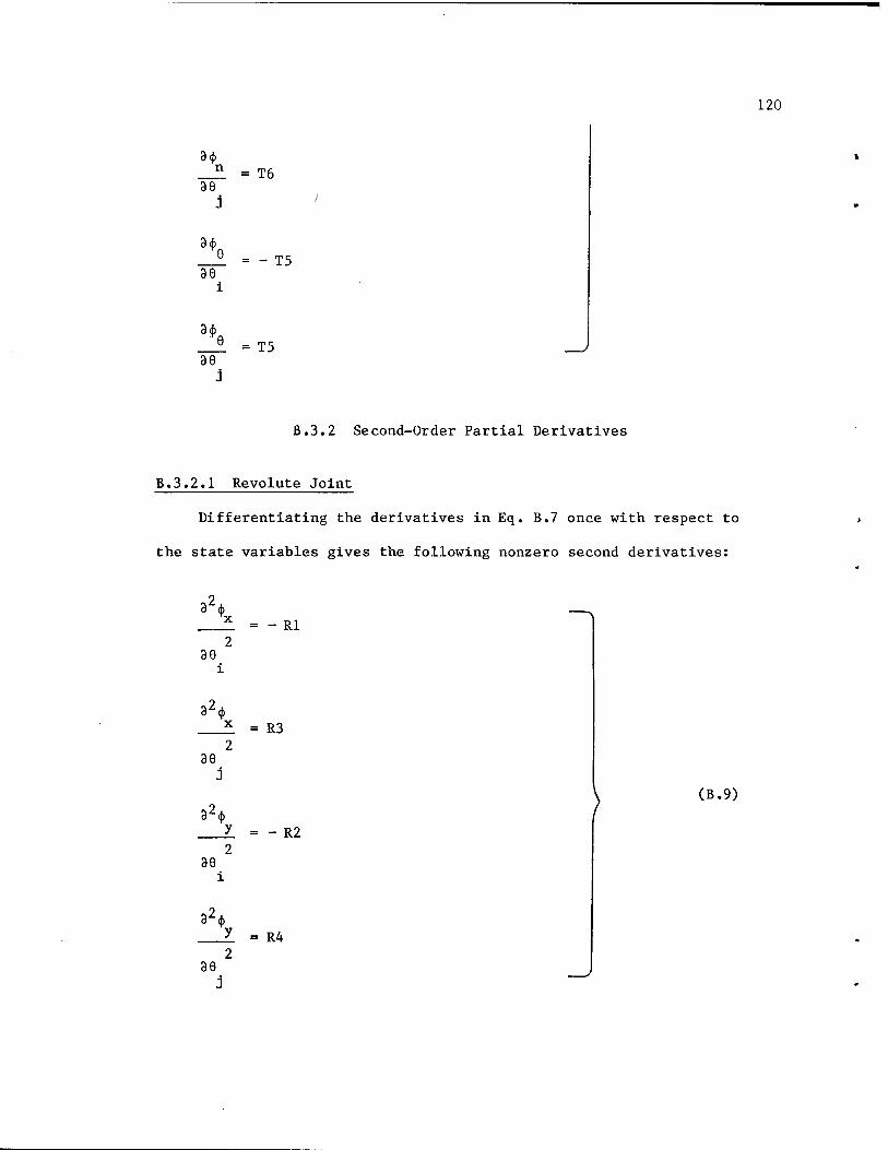
120

3(f) n

39 = T6

3<j)

39 = - T5

3(j) 6 _

39 = T5

B.3.2 Second-Order Partial Derivatives


Differentiating the derivatives in Eq. B.7 once with respect to

the state variables gives the following nonzero second derivatives:

32<|> x = - Rl

39

32<j) x _ R3

39

32<|)

(B.9)

Z = -R2

39

32<j> JL - R4

39

121


Differentiating the derivatives in Eq. B.8 with respect to state

variables gives the following nonzero second derivatives:

d <f> n

3x 39 i i

2 3 <j>

n 9y 30

i i

2 3 <j>

n 36 3x

i j

2 3 <f>

n 39 3y

i j

2 3 <f)

n 39 39

i J

2 3 <|>

n

= - T2

= T2

= T2

= - T2

= T5

= - (T1)(T7) - (T2)(T8) + T5

39

2 3 <t>

n = T5

39

(B.10)

122

2 8 4)

89

2 8 <j>

8

86 89 i j

2 8 <j>

= - T6

= T6

= - T6

89

B.3.3 Third-Order Partial Derivatives


Differentiating Eq. B.9 once with respect to state variables gives

the following nonzero third derivatives:

3 8 <|)

x = R2

89

3 8 <|>

89

R4

3 8 <|>

(B.ll)

JL = - Rl

89

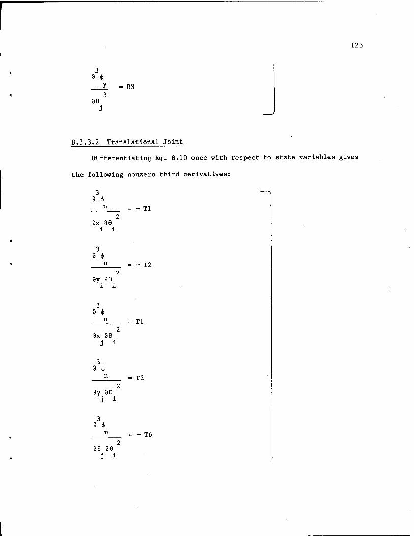
123

3 9 <t>

_y = R3

ae


Differentiating Eq. B.10 once with respect to state variables gives

the following nonzero third derivatives:

3 9 $

n

2 9x 99

l l

3 9 4

n

2 9y 96

i i

3 9 <j)

n

2 9x 90

J i

3 9 4>

n

2 9y 99

j i

3 9 $

n

2 99 99

j i

Tl

T2

= Tl

= T2

= - T6

124

3 3 <j>

n T6

89 39

3 8 <j>

n = (T2)(T7) - (T1)(T8) + T6

99

3 3 <}>

n = T6

39 (B.12)

3 3 <j>

9 = T5

39

3 3 $

9

2 39 39

i j

= - T5

3 3 <|>

9 = T5

39 39 i j

3 3 <t>

= - T5

39

125

B.4 Cross Derivatives With Respect to Design and State Variables

B.4.1 Second-Order Cross Partial Derivatives

B»4.1.1 Revolute Joint

Differentiating Eqs. B.7 once with respect to design variables the

following nonzero second-order cross partial derivatives result:

2 9 4>

X

89 9b i k

2 9 <(>

96 9b j k

. 2 9 4>

99 9b i k

RB2

= - RBI

RB4

2 3 i})

99 9b j k

2 9 <j>

99 9b i k

2 9 <|>

96 9b j k

= - RB3

= - TB5

= TB5

(B.13)

126


Differentiating Eq. B.8 with respect to design the following

nonzero second-order cross partial derivatives result:

2

n = TBl 3x 3b

i k

2 3 <f>

n = TB2 3y 3b

i k

2 3 $

n = - (TB2)(T7) - (T2 36 3b

i k + (T1)(TB8) - TB6

2 3 <(>

n = - TBl 3x 3b

2 3 <j)

n = - TB2 3y 3b

j k

2 3 <j>

n = TB6 36 3b

j k

(B.14)

127

B.4.2 Third-Order Cross Partial Derivatives


Differentiating the second-order derivatives in Eq. B.9 once with

respect to design gives the following nonzero third-order cross

partial derivatives:

3

X - RBI 2

90 3b i k

3 3 $

X RB3 2

39 3b

3 3 <|>

y - RB2 2

39 3b i k

3 3 <f>

y RB4 2

39 3b j k

(B.15)


Differentiating the second-order derivatives in Eq. B.10 once with

respect to design gives the following nonzero third-order partial cross

derivatives:

3 3 (j)

n 3x 39 3b

i i k

= - TB2

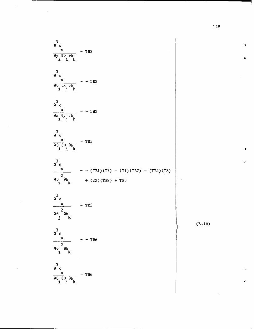
128

3 9 $

3y 86 9b i i k

= TB2

3 9 $

n 36 9x 9b

i j k

= - TB2

3 9 <(>

n 9x 9y 9b

i j k

= - TB2

3 9 <j>

n 96 96 9b

i 3 k

= TB5

3 9 <|>

2 99 9b

i k

- (TB1)(T7) - (T1)(TB7) - (TB2)(T8)

+ (T2)(TB8) + TB5

3 9 <j>

2 96 9b

j k

3 9 <j>

2 96 9b

i k

= TB5

= - TB6

(B.16)

3 9 <J>

n 96 96 9b

i j k

= TB6

129

3 3 (j)

n = - TB6 2

39 3b j k

DISTRIBUTION LIST

Please notify USATACOM, DRSTA-ZSA, Warren, Michigan 48090, of corrections and/or changes in address.

Commander (25) US Army Tk-Autmv Command R&D Center Warren, MI 48090

Superintendent (02) US Military Academy ATTN: Dept of Engineering

Course Director for Automotive Engineering

Commander (01) US Army Logistic Center Fort Lee, VA 23801

US Army Research Office (02) P.O. Box 12211 ATTN: Dr. F. Schmiedeshoff

Dr. R. Singleton Research Triangle Park, NC 27709

HQ, DA (01) ATTN: DAMA-AR

Dr. Herschner Washington. D.C. 20310

HQ, DA (01) Office of Dep Chief of Staff for Rsch, Dev & Acquisition ATTN: DAMA-AR

Dr. Charles Church Washington, D.C. 20310

HQ, DARCOM 5001 Eisenhower Ave. ATTN: DRCDE

Dr. R.L. Haley Alexandria, VA 22333

Director (01) Defense Advanced Research Projects Agency 1400 Wilson Boulevard Arlington, VA 22209

Commander (01) US Army Combined Arms Combat Developments Activity ATTN: ATCA-CCC-S Fort Leavenworth, KA 66027

Commander (01) US Army Mobility Equipment Research and Development Command ATTN: DRDME-RT Fort Belvoir, VA 22060

Director (02) US Army Corps of Engineers Waterways Experiment Station P.O. Box 631 Vicksburg, MS 39180

Commander (01) US Army Materials and Mechanics Research Center ATTN: Mr. Adachi Watertown, MA 02172

Director (03) US Army Corps of Engineers Waterways Experiment Station P.O. Box 631 ATTN: Mr. Nuttall Vicksburg, MS 39180

Director (04) US Army Cold Regions Research & Engineering Lab P.O. Box 282 ATTN: Dr. Freitag, Dr. W. Harrison Dr. Liston, Library Hanover, NH 03755

Grumman Aerospace Corp (02) South Oyster Bay Road ATTN: Dr. L. Karafiath

Mr. F. Markow M/S A08/35

Bethpage, NY 11714

Dr. Bruce Liljedahl (01) Agricultural Engineering Dept Purdue University Lafayette, IN 46207

Mr. H.C. Hodges (01) Nevada Automotive Test Center Box 234 Carson City, NV 89701

Mr. R.S. Wismer (01) Deere & Company Engineering Research 3300 River Drive Moline, IL 61265

Oregon State University (01) Library Corvallis, OR 97331

Southwest Research Inst (01) 8500 Culebra Road San Antonia, TX 78228

FMC Corporation (01) Technical Library P.O. Box 1201 San Jose, CA 95108

Mr. J. Appelblatt (01) Director of Engineering Cadillac Gauge Company P.O. Box 1027 Warren, MI 48090

CALSPAN Corporation (01) Box 235 Library 4455 Benesse Street Buffalo, NY 14221

SEM, (01) Forsvaretsforskningsanstalt Avd 2 Stockholm 80, Sweden

Mr. Hedwig (02) RU II1/6 Ministry of Defense 5300 Bonn, Germany

Foreign Science & Tech (01) Center 220 7th Street North East ATTN: AMXST-GEI

Mr. Tim Nix Charlottesville, VA 22901

General Research Corp (01) 7655 Old Springhouse Road Westgate Research Park ATTN: Mr. A. Viilu McLean, VA 22101

Commander (01) US Army Developmant and Readiness Command 5001 Eisenhower Avenue ATTN: Dr. R.S. Wiseman Alexandria, VA 22333

Chrysler Corporation (02) Mobility Research Laboratory, Defense Engineering Department 6100 P.O. Box 751 Detroit, MI 48231

President (02) Army Armor and Engineer Board Fort Knox, KY 40121

Commander (01) US Army Arctic Test Center APO 409 Seattle, WA 98733

Commander (02) US Army Test & Evaluation Command ATTN: AMSTE-BB and AMSTE-TA Aberdeen Proving Ground, MD 21005

Commander (01) US Army Armament Research and Development Command ATTN: Mr. Rubin Dover, NJ 07801

Commander (01) US Army Yuma Proving Ground ATTN: STEYP-RPT Yuma, AZ 85364

Commander (01) US Army Natic Laboratories ATTN: Technical Library Natick, MA 01750

Director (01) US Army Human Engineering Lab ATTN: Mr. Eckels Aberdeen Proving Ground, MD 21005

Director (02) US Army Ballistic Research Lab Aberdeen Proving Ground, MD 21005

Director (02) US Army Materiel Systems Analysis Agency ATTN: AMXSY-CM Aberdeen Proving Ground, MD 21005

Director (02) Defense Documentation Center Cameron Station Alexandria, VA 22314

US Marine Corps (01) Mobility & Logistics Division Development and Ed Command ATTN: Mr. Hickson Quantico, VA 22134

Keweenaw Field Station (01) Keweenaw Research Center Rural Route 1 P.O. Box 94-D ATTN: Dr. Sung M. Lee Calumet, MI 49913

Naval Ship Research & (02) Dev Center Aviation & Surface Effects Dept Code 161 Washington, D.C. 20034

Director (01) National Tillage Machinery Lab Box 792 Auburn, AL 36830

Director (02) USDA Forest Service Equipment Development Center 444 East Bonita Avenue San Dimes, CA 91773

Engineering Societies Library 345 East 47th Street New York, NY 10017

(01)

(01) Dr. I.R. Erlich Dean for Research Stevens Institute of Technology Castle Point Station Hoboken, NJ 07030

n t yk - defense technical information center t yk la boratory ... of a four-bar mechanism 82 5.4.1...

Documents