macroeconometric modelling of in dynamics and …folk.uio.no/rnymoen/eommsupply.pdf ·...
TRANSCRIPT
Macroeconometric Modelling of InflationDynamics and Unemployment
Equilibrium∗
Ragnar NymoenUniversity of Oslo
Department of Economics
This version 3. June 2003 (first version 21 Jan 2003)
Contents
1 Introduction and overview 1
2 The Norwegian main-course model 52.1 Cointegration . . . . . . . . . . . . . . . . . . . . . . . . . . . . . . . 62.2 Causality . . . . . . . . . . . . . . . . . . . . . . . . . . . . . . . . . 102.3 Steady state growth . . . . . . . . . . . . . . . . . . . . . . . . . . . . 112.4 Early empiricism . . . . . . . . . . . . . . . . . . . . . . . . . . . . . 112.5 Summary . . . . . . . . . . . . . . . . . . . . . . . . . . . . . . . . . 12
3 The Phillips curve 133.1 Lineages of the Phillips curve . . . . . . . . . . . . . . . . . . . . . . 133.2 Cointegration, causality and the Phillips curve natural rate . . . . . 143.3 Is the Phillips curve consistent with persistent changes in unemploy-
ment? . . . . . . . . . . . . . . . . . . . . . . . . . . . . . . . . . . . 183.4 Estimating the uncertainty of the Phillips curve NAIRU . . . . . . . 213.5 Inversion and the Lucas critique . . . . . . . . . . . . . . . . . . . . . 22
3.5.1 Inversion . . . . . . . . . . . . . . . . . . . . . . . . . . . . . . 23
∗Section 2- 6 are draft versions of chapter 3-7 in “Econometrics of Macroeconomic Modelling”by Eitrheim, Bårdsen, Jansen and Nymoen, which is forthcoming on Oxford University Press.Section 6 is co-authored with Gunnar Bårdsen and Eilev Jansen. Comments are welcome! e-mail:[email protected]
i
3.5.2 Lucas critique . . . . . . . . . . . . . . . . . . . . . . . . . . . 233.5.3 Model-based versus data-based expectations . . . . . . . . . . 253.5.4 Testing the Lucas critique . . . . . . . . . . . . . . . . . . . . 27
3.6 An empirical open economy Phillips curve system . . . . . . . . . . . 283.7 Summary . . . . . . . . . . . . . . . . . . . . . . . . . . . . . . . . . 38
4 Wage bargaining and price setting 394.1 Wage bargaining and monopolistic competition . . . . . . . . . . . . 394.2 The wage curve NAIRU . . . . . . . . . . . . . . . . . . . . . . . . . 434.3 Cointegration and identification. . . . . . . . . . . . . . . . . . . . . . 444.4 Cointegration and Norwegian manufacturing wages. . . . . . . . . . . 474.5 Aggregate wages and prices: UK quarterly data. . . . . . . . . . . . . 514.6 Summary . . . . . . . . . . . . . . . . . . . . . . . . . . . . . . . . . 52
5 Wage-price dynamics 545.1 Nominal rigidity and equilibrium correction . . . . . . . . . . . . . . 545.2 Stability and steady state . . . . . . . . . . . . . . . . . . . . . . . . 565.3 The stable solution of the conditional wage-price system . . . . . . . 58
5.3.1 Cointegration, long run multipliers and the steady state . . . . 605.3.2 Nominal rigidity despite dynamic homogeneity . . . . . . . . . 615.3.3 An important unstable solution: the “no wedge” case . . . . . 625.3.4 A main-course interpretation . . . . . . . . . . . . . . . . . . . 64
5.4 Comparison with the wage-curve NAIRU . . . . . . . . . . . . . . . . 655.5 Comparison with the wage Phillips curve NAIRU . . . . . . . . . . . 675.6 Do estimated wage-price models support the NAIRU view of equilib-
rium unemployment? . . . . . . . . . . . . . . . . . . . . . . . . . . . 685.6.1 Empirical wage equations . . . . . . . . . . . . . . . . . . . . 685.6.2 Aggregate wage-price dynamics in the UK. . . . . . . . . . . . 70
5.7 Econometric evaluation of Nordic structural employment estimates . 705.7.1 The NAWRU . . . . . . . . . . . . . . . . . . . . . . . . . . . 725.7.2 Do NAWRU fluctuations match up with structural changes in
wage formation? . . . . . . . . . . . . . . . . . . . . . . . . . 735.7.3 Summary of time varying NAIRUs in the Nordic countries . . 77
5.8 Beyond the natural rate doctrine: Unemployment-inflation dynamics 785.8.1 A complete system . . . . . . . . . . . . . . . . . . . . . . . . 795.8.2 Wage-price dynamics: Norwegian manufacturing . . . . . . . . 80
5.9 Summary . . . . . . . . . . . . . . . . . . . . . . . . . . . . . . . . . 86
6 The New Keynesian Phillips curve 876.1 A NPC system . . . . . . . . . . . . . . . . . . . . . . . . . . . . . . 886.2 European inflation and the NPC . . . . . . . . . . . . . . . . . . . . . 926.3 Tests and empirical evaluation: US and ‘Euroland’ data . . . . . . . . 95
6.3.1 Goodness-of-fit . . . . . . . . . . . . . . . . . . . . . . . . . . 956.3.2 Tests of significance of the forward term . . . . . . . . . . . . 986.3.3 Tests based on the closed form solution (Rudd-Whelan test) . 1026.3.4 Test based on the transformed closed form solution . . . . . . 1036.3.5 Evaluation of the NPC system . . . . . . . . . . . . . . . . . 104
ii
6.4 NPC and inflation in small open economies. Testing the encompassingimplications . . . . . . . . . . . . . . . . . . . . . . . . . . . . . . . . 1066.4.1 The encompassing implications of the NPC . . . . . . . . . . . 1076.4.2 Norway . . . . . . . . . . . . . . . . . . . . . . . . . . . . . . 1086.4.3 United Kingdom . . . . . . . . . . . . . . . . . . . . . . . . . 109
6.5 Summary . . . . . . . . . . . . . . . . . . . . . . . . . . . . . . . . . 111
A Lucas critique (Chapter 3.5) 112
B Solution and estimation of simple rational expectations models 112B.1 Model with forward looking term only . . . . . . . . . . . . . . . . . 113
B.1.1 Roots . . . . . . . . . . . . . . . . . . . . . . . . . . . . . . . 113B.1.2 Solution . . . . . . . . . . . . . . . . . . . . . . . . . . . . . . 114B.1.3 Estimation . . . . . . . . . . . . . . . . . . . . . . . . . . . . . 115
B.2 Hybrid model with both forward and backward looking terms . . . . 116B.2.1 Roots . . . . . . . . . . . . . . . . . . . . . . . . . . . . . . . 116
B.3 Does the MA(1) process prove that the forward solution applies? . . . 116
C Data used in Chapter 3-5 118C.1 Annual data set for Norwegian manufacturing wages. . . . . . . . . . 118C.2 United Kingdom, quarterly wage and price data. . . . . . . . . . . . . 119
D Data used in used in section 6 119D.1 The Euroland data . . . . . . . . . . . . . . . . . . . . . . . . . . . . 119
D.1.1 The basic series from ECB . . . . . . . . . . . . . . . . . . . . 119D.1.2 Data used to replicate GGL (sections 6.1 and 6.3.1) . . . . . . 120D.1.3 Data used in sections 6.3.3 - 6.3.5 . . . . . . . . . . . . . . . 120
D.2 The U.S. data . . . . . . . . . . . . . . . . . . . . . . . . . . . . . . . 120D.2.1 The source data . . . . . . . . . . . . . . . . . . . . . . . . . . 120D.2.2 Data used in section 6.3.1 . . . . . . . . . . . . . . . . . . . . 120
D.3 The Norwegian data . . . . . . . . . . . . . . . . . . . . . . . . . . . 120D.3.1 Notes . . . . . . . . . . . . . . . . . . . . . . . . . . . . . . . 120D.3.2 Definitions . . . . . . . . . . . . . . . . . . . . . . . . . . . . . 121
D.4 The UK data . . . . . . . . . . . . . . . . . . . . . . . . . . . . . . . 122D.4.1 The source data for the Bank of England study . . . . . . . . 122D.4.2 Bank of England variables used in section 6.4.3 . . . . . . . . 122D.4.3 Variables used to calculate the error correction terms in sec-
tion 6.4.3 . . . . . . . . . . . . . . . . . . . . . . . . . . . . . 122
iii
1 Introduction and overview
In the course of the 1980s and 1990s the supply side of macroeconometric modelsreceived increased attention, correcting the earlier over-emphasis on the demandside of the economy. Although there are many facets of the “supply side”, e.g.,price setting, labour demand and investment in fixed capital and R&D, the maintheoretical and methodological developments and controversies have been focusedon wage and price setting.
Arguably, the most important conceptual development in this area have beenthe Phillips curve–the relationship between the rate of change in money wages andthe rate of unemployment, Phillips (1958),–and the “natural rate of unemployment”hypothesis, Phelps (1967) and Friedman (1968). Heuristically, the natural ratehypothesis says that there is only one unemployments rate that can be reconciledwith nominal stability of the economy (constant rates of wage and price inflation).Moreover, the natural rate equilibrium is asymptotically stable. Thus natural ratehypothesis contradicted the demand driven macroeconometric models of its day,which implied that the rate of unemployment could be kept at any (low) level bymeans of fiscal policy. A step towards reconciliation of the conflicting views wasmade with the discovery that a constant (“structural”) natural rate is not necessarilyinconsistent with a demand driven (“Keynesian”) model. The trick was to introducean “expectations augmented” Phillips-curve relationship into a IS-LM type model.The modified model left considerable scope for fiscal policy in the short run, butdue to the Phillips curve, a long term natural rate property was implied, see e.g.,Calmfors (1977).
However, a weak point of the synthesis between the natural rate and the Keyne-sian models was that the supply side equilibrating mechanisms were left unspecifiedand open to interpretation. Thus, new questions came to the forefront, like: Howconstant is the natural rate? Is the concept inextricably linked to the assumption ofperfect competition, or is it robust to more realistic assumptions about market formsand firm behaviour, such as monopolistic competition? And what is the impact ofbargaining between trade unions and confederations over wages and work condi-tions, which in some countries has given rise to a high degree of centralization andcoordination in wage setting? Consequently, academic economists have discussedthe theoretical foundations and investigated the logical, theoretical and empiricalstatus of the natural rate hypothesis, as for example in the contributions of Layardet al. (1991, 1994), Cross (1988, 1995), Staiger et al. (1997) and Fair (2000).
In the current literature, the term “Non-Accelerating Inflation Rate of Unem-ployment”, or NAIRU, is used as a synonym to the “natural rate of unemployment”.Historically, the need for a new term arose because the macroeconomics rhetoric ofthe natural rate suggested inevitability, which is something of a strait jacket since thelong run rate of unemployment is almost certainly conditioned by socio-economicfactors, policy and institutions, see e.g., Layard et al. (1991, Chapter 1.3).1 Theacronym NAIRU itself is something of a misnomer since taken literally it implies...p ≤ 0 where p is the log of the price level. However, as a synonym for the nat-ural rate it implies p = 0, which would be CIRU (constant rate of inflation rate of
1See Cross (1995, p. 184), who notes that an immutable and unchangeable natural rate wasnot implied by Friedman (1968).
1
unemployment). We follow established practice and use the natural rate - NAIRUterminology in the following.
There is little doubt that the natural rate counts as one of the most successfulconcepts in the history of macroeconomics. Governments and international organi-zations customarily refer to NAIRU calculations in their discussions of employmentand inflation prospects2, and the existence of a NAIRU consistent with a verticallong-run Phillips curve is crucial to the framework of monetary policy.3
The 1980s saw a marked change in the consensus view on the model suitable forderiving NAIRU measures. There was a shift away from a Phillips curve frameworkthat allowed estimation of a natural rate NAIRU from a single equation for the rateof change of wages (or prices). The new approach combined a negative relationshipbetween the level of the real wage and the rate of unemployment, dubbed the wagecurve by Blanchflower and Oswald (1994), with an equation representing firms’ pricesetting. The wage curve is consistent with a wide range of economic theories, seeBlanchard and Katz (1997), but its original impact among European economistswas due to the explicit treatment of union behaviour and imperfectly competitiveproduct markets, pioneered by Layard and Nickell (1986). In the same decade, timeseries econometrics constituted itself as a separate branch of econometrics, with itsown methodological issues, controversies and solutions, as explained in Part 1. It isinteresting to note how early new econometric methodologies are applied to wage-price modelling, e.g., error-correction modelling, the Lucas-critique, cointegrationand dynamic modelling. Thus, wage formation became an area where economictheory and econometric methodology intermingled fruitfully. In this section wedraw on these developments when we discuss how the different theoretical modelsof wage formation and price setting can be estimated and evaluated empirically.
The move from the Phillips curve to a wage curve in the 1980s was howevermainly a European phenomenon. The Phillips curve held its ground very well inthe USA, see Fuhrer (1995), Gordon (1997) and Blanchard and Katz (1999). Butalso in Europe the case has been re-opened. For example, Manning (1993) showedthat a Phillips curve specification is consistent with union wage setting, and thatthe Layard-Nickell wage equation was not identifiable. The Bank of England (1999)includes Phillips-curve models in their suite of models for monetary policy. However,the telling revitalization of the Phillips curve is due to its prolific role in New Key-nesian macroeconomics and in the modern theory of monetary policy in general, seeSvensson (2000). The defining characteristics of the New Keynesian Phillips (NPC)curve are strict microeconomic foundations together with rational expectations of“forward” variables, Clarida et al. (1999) and Galí et al. (2001a).
There is a long list of issues connected to the idea of a supply side determinedNAIRU, e.g., the existence and estimation of such an entity, and its eventual corre-spondence to a steady state solution of a larger system explaining wages, prices aswell as real output and labour demand and supply. However, at an operational level,the NAIRU concept is model dependent. Thus, the NAIRU-issues cannot be seenas separated from the wider question of choosing a framework for modelling wage,
2See Elmeskov and MacFarland (1993), Scrapetta (1996) and OECD (1997c, Chapter 1) forexamples.
3See the discussion in King (1998) for a central banker’s views.
2
price and unemployment dynamics in open economies. In the following sections wetherefore give an appraisal of what we see as the most important macroeconomicmodels in this area. We cover more than 40 years of theoretical developments, star-ing with the Norwegian (aka Scandinavian) model of inflation of the early sixties,followed by the Phillips curve models of the 1970s and ending up with the modernincomplete competition model and the New Keynesian Phillips curve.
In reviewing the sequence of models, we find examples of newer theories thatgeneralize on the older models that they supplant, as one would hope in any field ofknowledge. However, just as often new theories seem to arise and become fashionablebecause they, by way of specialization, provide a clear answer on issues that oldertheories left in the vague. The underlying process at work here is that as societyevolve, new issues enter the agenda of politicians and their economic advisers. Forexample, the Norwegian model of inflation, though rich in insight about how the rateof inflation can be stabilized (i.e. p = 0), does not count the adjustment of the rate ofunemployment to its natural rate as even a necessary requirement for p = 0. Clearly,this view is conditioned by a socioeconomic situation in which “full employment”with moderate inflation was seen as attainable and almost a ‘natural’ situation. Incomparison, both the Phelps/Friedman Phillips curve model of the natural rate, andthe Layard-Nickell NAIRU model specialize their answers to the same question, andtakes for granted that it is necessary for p = 0 that unemployment equals a naturalrate or NAIRU which is entirely determined by long run supply factors.
Just as the Scandinavian model’s vagueness about the equilibrating role ofunemployment must be understood in a historical context, it quite possible that thenatural rate thesis is a product of socioeconomic developments. However, while rela-tivism is an interesting way of understanding the origin and scope of macroeconomictheories, we do not share Dasgupta’s (1985) extreme relastivistic stance, i.e., thatsuccessive theories belong to different epochs, each defined by their answers to a newset of issues, and that one cannot speak of progress in economics. On the contrary,our position is that the older models of wage-price inflation and unemployment oftenrepresent insights that remain of interest today.
Section 2 starts with a re-construction of the Norwegian model of inflation, interms of modern econometric concepts of cointegration and causality. Today thismodel, which stems back to the 1960s, is little known outside Norway. Yet, in itsre-constructed forms it is almost a time traveller, and in many respects resemblesthe modern theory of wage formation with unions and price setting firms. In itstime, the Norwegian model of inflation was viewed as a contender to the Phillipscurve, and in retrospect it is easy to see that the Phillips curve won. However,the Phillips curve and the Norwegian model are in fact not mutually exclusive.A conventional open economy version of the Phillips curve can be incorporatedinto the Norwegian model, and in section 3 we approach the Phillips curve fromthat perspective. However, the bulk of the section concerns issues that is quiteindependent of the connection between the Phillips curve and the Norwegian modelof inflation. As perhaps the ultimate example of a consensus model in economics, thePhillips curve also became a focal point for developments in both economic theoryand in econometrics. In particular we focus on the development of the natural ratedoctrine, and on econometric advances and controversies related to the stability ofthe Phillips curve (the origin of the Lucas critique).
3
As mentioned above, the Phillips curve has recently lost some of its position tothe Layard-Nickell wage curve model, which we discuss in section 4, before section 5presents a unifying framework of the two models (as well as the Norwegian model).In that section, we also discuss at some length the NAIRU doctrine: Is it a straitjacket for macroeconomic modelling, or an essential ingredient? Is it a truism, orcan it be tested? What can put in its place if it is rejected? We think that wegive answers to all this questions, and that the thrust of the argument represents anintellectual rationale for macroeconometric modelling of larger systems-of-equations.
An important underlying assumption of section 2-5 is that inflation and unem-ployment follow causal or future-independent processes, see Brockwell and Davies(1991, Chapter 3), meaning that the roots of the characteristic polynomials of thedifference equations are inside the unit circle. This means that all the different eco-nomic models can be represented within the framework of linear difference equationswith constant parameters. Thus the econometric framework is the vector autore-gressive model (VAR), and identified systems of equations that encompass the VAR,see Hendry and Mizon (1993), Bårdsen and Fisher (1999). Non-stationarity is as-sumed to be of a kind that can be modelled away by differencing, by establishingcointegrating relationships, or by inclusion of deterministic dummy variables in thenon-homogenous part of the difference equations.
In section 6 we discuss the New Keynesian Phillips curve (NPC) of Galí andGertler (1999), where the stationary solution for the rate of inflation involves leads(rather than lags) of the non-modelled variables. However, non-causal stationarysolutions could also exists for the “older” price-wage models in section 2-5, i.e., ifthey are specified with “forward looking” variables, see Wren-Lewis and Moghadam(1994). Thus, the discussion of testing issues related to forward versus backwardlooking models in section 6 is relevant for a wider class of forward-looking models,not just the New Keynesian Phillips curve.
The role of money in the inflation process is an old issue in macroeconomics, yetmoney play no essential part in the models surveyed in the following. This is because,despite the very notable differences existing between them, the models all subscribeto the same overall view of inflation: namely that inflation is best understood asa complex socioeconomic phenomenon reflecting imbalances in product and labourmarkets, and generally the level of conflict in society. This is inconsistent withe.g., a simple quantity theory of inflation, but arguably not with having excessdemand for money as a source of inflation pressure. In the book The Econometricsof Macroeconomic Modelling we use that perspective to investigate the relationshipbetween money demand and supply and inflation
Econometric analysis of wage, price and unemployment data serve to sub-stantiate the discussion in this part of the book. An annual data set for Norwayis used throughout section 3-5 to illustrate the application of three main models(Phillips curve, wage curve, and wage price dynamics) to a common dataset. Butfrequently we also present analysis of data from the other Nordic countries, as wellas of quarterly data from UK and USA and ‘Euroland’ and Norway.
4
2 The Norwegian main-course model
The Scandinavian model of inflation was formulated in the 1960s4. It became theframework for both medium term forecasting and normative judgements about “sus-tainable” centrally negotiated wage growth in Norway.5 In this section we show thatAukrust’s (1977) version of the model can be reconstructed as a set of propositionsabout cointegration properties and causal mechanisms.6 The reconstructed Norwe-gian model serves as a reference point for, and in some respects also as a correctiveto, the modern models of wage formation and inflation in open economies, e.g., theopen economy Phillips curve and the imperfect competition model of e.g., Layardand Nickell (1986), section 3.2 and 4. It also motivates our generalization of thesemodels in section 5.8.2.
Central to the model is the distinction between a tradables sector where firmsact as price takers, either because they sell most of their produce on the worldmarket, or because they encounter strong foreign competition on their domesticsales markets, and a non-tradeables sector where firms set prices as mark-ups onwage costs. In equations (2.4)-(2.8), we,t denotes the nominal wage in the tradeableor exposed (e) industries in period t. qe,t and ae,t are the product price and averagelabour productivity of the exposed sector. ws,t, qs,t and as,t are the correspondingvariables of the non-tradeables or sheltered (s) sector.7 Finally, pt is the consumerprice. All variables are measured in natural logarithms, so e.g., wt = log(Wt) for
4In fact there were two models, a short-term multisector model, and the long-term two sectormodel that we re-construct using modern terminology in this chapter. The models were formulatedin 1966 in two reports by a group of economists who were called upon by the Norwegian governmentto provide background material for that year’s round of negotiations on wages and agriculturalprices. The group (Aukrust, Holte and Stolzt) produced two reports. The second (dated October20 1966, see Aukrust (1977)) contained the long-term model that we refer to as the main-coursemodel. Later, there was similar development in e.g., Sweden, see Edgren et al. (1969) and theNetherlands, see Driehuis and de Wolf (1976).In later usage the distinction between the short and long-term models seems to have become
blurred, in what is often referred to as the Scandinavian model of inflation. We acknowledgeAukrust’s clear exposition and distinction in his 1977 paper, and use the name Norwegian maincourse model for the long-term version of his theoretical framework.
5On the role of the main-course model in Norwegian economic planning, see Bjerkholt (1998).6For an exposition and appraisal of the Scandinavian model in terms of current macroeconomic
theory, see Rødseth (2000, Chapter 7.6).7In France, the distinction between sheltered and exposed industries became a feature of models
of economic planning in the 1960s, and quite independently of the development in Norway. In fact,in Courbis (1974), the main-course theory is formulated in detail and illustrated with data fromFrench post war experience (we are grateful to Odd Aukrust for pointing this out to us).
5
the wage rate.
qe,t = pft + υ1,t(2.1)
pft = gf + pft−1 + υ2,t(2.2)
ae,t = gae + ae,t−1 + υ3,t(2.3)
we,t − qe,t − ae,t = me + υ4,t(2.4)
we,t = ws,t + υ5,t(2.5)
as,t = gas + as,t−1 + υ6,t(2.6)
ws,t − qs,t − as,t = ms + υ7,t(2.7)
pt = φqs,t + (1− φ)qe,t, 0 < φ < 1.(2.8)
gi(i = f , ae, as) are constant growth rates, mi(i = e, s) are means of the logarithmsof the wage shares in the two industries and φ is a coefficient that reflects the weightof non-traded goods in private consumption.8
The seven stochastic processes υ1,t (i = 1, ...7) play a key role in our recon-struction of Aukrust’s theory. They represent separate ARMA processes. The rootsof the associated characteristic polynomials are assumed to lie on or outside theunit-circle. Hence,υ1,t (i = 1, ...7) are causal ARMA processes, cf. Brockwell andDavies (1991).
2.1 CointegrationEquation (2.1) defines the price taking behaviour characterizing the exposed indus-tries and (2.2)-(2.3) define foreign prices (pft) and labour productivity as randomwalks with drifts. Equation (2.4) serves a double function: First, it defines the ex-posed sector wage share we,t−qe,t−ae,t as a stationary variable since υ4,t on the righthand side is I(0) by assumption. Second, since both qe,t and ae,t are I(1) variables,the nominal wage we,t is also non-stationary I(1).
The sum of the technology trend and the foreign price plays an important rolein the theory since it traces out a central tendency or long run sustainable scopefor wage growth. Aukrust (1977) aptly refers to this as the main-course for wagedetermination in the exposed industries. Thus, for later use we define the maincourse variable: mct = ae,t+ qe,t. The essence of the statistical interpretation of thetheory is captured by the assumption that υ1,t is ARMA. It follows that we,t andmct are cointegrated, that the difference between we,t and mct has a finite variance,and that deviations from the main course will lead to equilibrium correction in we,t,see Nymoen (1989a) and Rødseth and Holden (1990).
Hypothetically, if shocks were switched off from period 0 and onwards, thewage level would follow the deterministic function
(2.9) E[we,t | mc0] = me + (gf + gae)t+mc0, mc0 = pf0 + ae,0, (t = 1, 2, ...).
The variance of we,t is unbounded, reflecting the stochastic trends in productivityand foreign prices, thus we,t ∼ I(1).
8Note that, due to the log-form, φ = xs/(1 − xs) where xs is the share of non-traded good inconsumption.
6
In his 1977 paper, Aukrust identifies the “controlling mechanism” in equation(2.4) as fundamental to his theory. Thus for example:
The profitability of the E industries is a key factor in determining thewage level of the E industries: mechanism are assumed to exist whichensure that the higher the profitability of the E industries, the highertheir wage level; there will be a tendency of wages in the E industries toadjust so as to leave actual profits within the E industries close to a “nor-mal” level (for which however, there is no formal definition). (Aukrust,1977, p 113).
In our reconstruction of the theory, the normal rate of profit is simply 1 − me.Aukrust also carefully states the long-term nature of his hypothesized relationship:
The relationship between the “profitability of E industries” and the“wage level of E industries” that the model postulates, therefore, is acertainly not a relation that holds on a year-to-year basis”. At best it isvalid as a long-term tendency and even so only with considerable slack.It is equally obvious, however, that the wage level in the E industries isnot completely free to assume any value irrespective of what happens toprofits in these industries. Indeed, if the actual profits in the E industriesdeviate much from normal profits, it must be expected that sooner orlater forces will be set in motion that will close the gap. (Aukrust, 1977,p 114-115).
Aukrust goes on to specify “three corrective mechanisms”, namely wage negotia-tions, market forces (wage drift, demand pressure) and economic policy. If we inthese quotations substitute “considerable slack” with “υ1,t being autocorrelated butI(0)”, and “adjustment” and “corrective mechanism” with “equilibrium correction”,it is seen how well the concepts of cointegration and equilibrium correction matchthe gist of Aukrust’s original formulation. Conversely, the use of growth rates ratherthan levels, which became common in both text book expositions of the theory andin econometric work claiming to test it, see section 2.4, misses the crucial pointabout a low frequency, long-term relationship between foreign prices, productivityand exposed sector wage setting.
7
log wage level
time
Main course
"Upper boundary"
"Lower boundary"
0
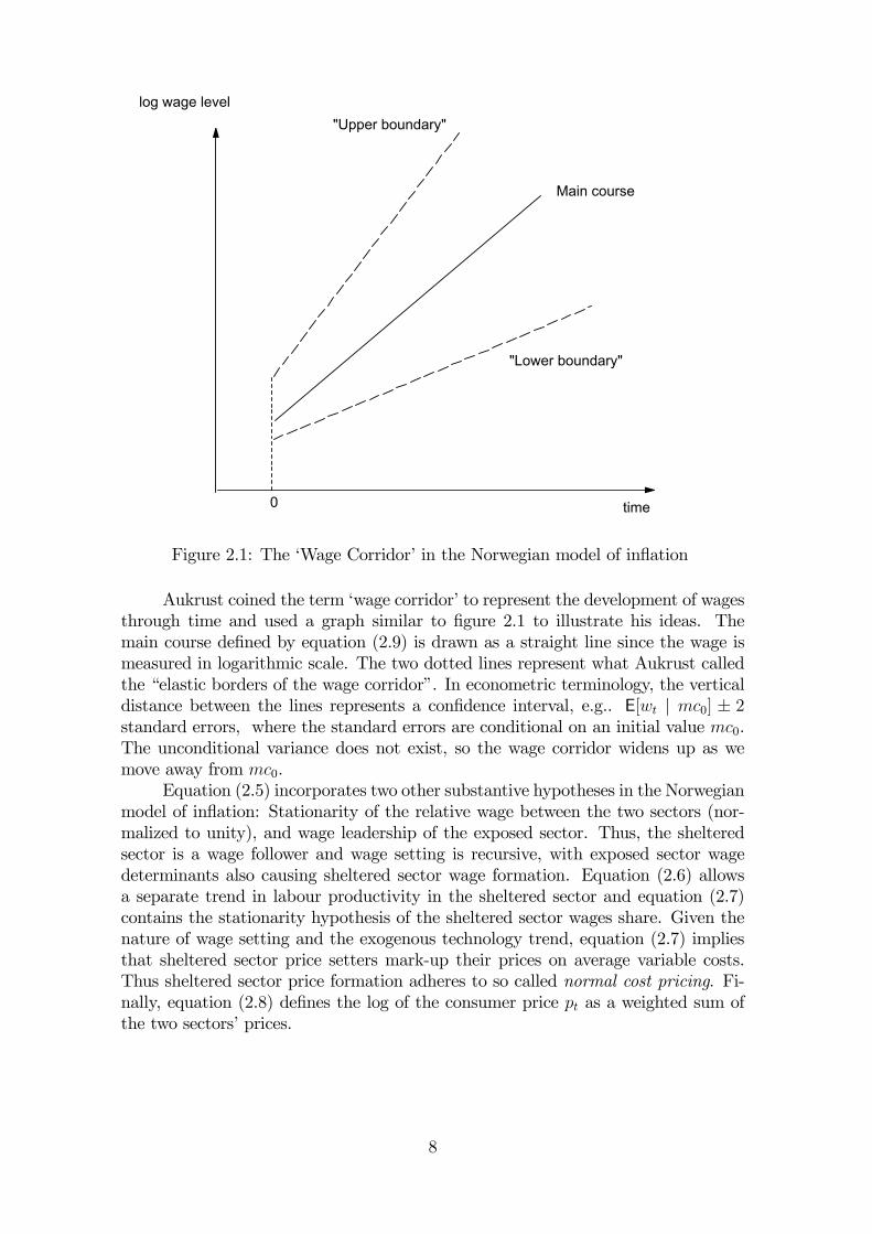
Figure 2.1: The ‘Wage Corridor’ in the Norwegian model of inflation
Aukrust coined the term ‘wage corridor’ to represent the development of wagesthrough time and used a graph similar to figure 2.1 to illustrate his ideas. Themain course defined by equation (2.9) is drawn as a straight line since the wage ismeasured in logarithmic scale. The two dotted lines represent what Aukrust calledthe “elastic borders of the wage corridor”. In econometric terminology, the verticaldistance between the lines represents a confidence interval, e.g.. E[wt | mc0] ± 2standard errors, where the standard errors are conditional on an initial value mc0.The unconditional variance does not exist, so the wage corridor widens up as wemove away from mc0.
Equation (2.5) incorporates two other substantive hypotheses in the Norwegianmodel of inflation: Stationarity of the relative wage between the two sectors (nor-malized to unity), and wage leadership of the exposed sector. Thus, the shelteredsector is a wage follower and wage setting is recursive, with exposed sector wagedeterminants also causing sheltered sector wage formation. Equation (2.6) allowsa separate trend in labour productivity in the sheltered sector and equation (2.7)contains the stationarity hypothesis of the sheltered sector wages share. Given thenature of wage setting and the exogenous technology trend, equation (2.7) impliesthat sheltered sector price setters mark-up their prices on average variable costs.Thus sheltered sector price formation adheres to so called normal cost pricing. Fi-nally, equation (2.8) defines the log of the consumer price pt as a weighted sum ofthe two sectors’ prices.
8
To summarize, the three basic cointegration propositions of the reconstructedmain course model are:
H1mc we,t − qe,t − ae,t = me + υ4,t, υ4,t ∼ I(0),H2mc we,t = ws,t + υ5,t, υ5,t ∼ I(0),H3mc ws,t − qs,t − as,t = ms + υ7,t, υ7,t ∼ I(0)
H1mc states that the exposed sector wage level cointegrates with the sectorial priceand productivity levels, with unit coefficients and for a constant mean of the wageshare,me. However, the institutional arrangements surrounding wage setting changesover time, so heuristically me may be time dependent. For example, bargainingpower and unemployment insurance systems are not constant factors but evolveover time, sometimes abruptly too. Aukrust himself, in his summary of the ev-idence for the theory, noted that the assumption of a completely constant meanwage share over long time spans was probably not tenable. However, no internalinconsistency is caused by replacing the assumption of unconditionally stationarywage shares with the weaker assumption of conditional stationarity. Thus, we con-sider in the following an extended main course model where the mean of the wageshare is a linear function of exogenous I(0) variables and of deterministic terms.
For example, a plausible generalization of H1mc is represented by
H1gmc we,t − qe,t − ae,t = me,0 + βe,1ut + βe,2Dt + υ4,t,
where ut is the log of the rate of unemployment and Dt is a dummy (vector) thatalong with ut help explain shifts in the mean of the wage share, thus in H1gmc,me,0 denotes the mean of the cointegration relationship, rather than of the wageshare itself. Consistency with the main course theory requires that the rate ofunemployment is interpreted as I(0), but not necessarily stationary, since ut may inturn be subject to changes in its mean, i.e., structural breaks. Graphically, the maincourse in figure 2.1 is no longer necessarily a straight unbroken line (unless the rateof unemployment and Dt stay constant for the whole time period considered).
Other candidate variables for inclusion in an extended main course hypothesisinclude the ratio between unemployment insurance payments and earnings (the socalled replacement ratio), and variables that represent unemployment compositioneffects (unemployment duration, the share of labour market programmes in totalunemployment), see Nickell (1987), Calmfors and Forslund (1991). In section 4 weshall see that in this extended form, the cointegration relationship implied by themain course model is fully consistent with modern wage bargaining theory.
Following the influence of trade union and bargaining theory, it has also becomepopular to estimate real-wage equations that include a so called wedge betweenreal wages and the consumer real wage, i.e., pt − qe,t in the present framework.However, inclusion of a wedge variable in the cointegrating wage equation of anexposed sector is inconsistent with the main-course hypothesis, and finding such aneffect empirically may be regarded as evidence against the framework. On the otherhand, there is nothing in the main-course theory that rules out substantive shortrun influences of the consumer price index. In section 5 we analyze a model thatcontains richer short run dynamics..
The other two cointegration propositions (H2mc and H3mc) in Aukrust’s modelhave not received nearly as much attention as H1mc in empirical research, but excep-tions include Rødseth and Holden (1990) and Nymoen (1991). In part, this is due to
9
lack of high quality data wage and productivity data and for the private service andretail trade sectors. Another reason is that both economists and policy makers inthe industrialized countries place most emphasis on understanding and evaluatingwage setting in manufacturing, because of its continuing importance for the overalleconomic performance.
2.2 CausalityThe main-course model specifies the following three hypothesis about causation:
H4mc mct → we,t,H5mc we,t → ws,t,H6mc ws,t → pt,
where→ denotes one-way causation. Causation may be contemporaneous or of theGranger-causation type. In any case the defining characteristic of the Norwegianmodel is that there is no feed-back between for example domestic cost of living(pt) and the wage level in the exposed sector. In his 1977 paper, Aukrust sees thecausation part of the theory (H4mc-H6mc) as just as important as the long term“controlling mechanism” (H1mc-H3mc). If anything Aukrust seems to put extraemphasis on the causation part. For example, he argues that exchange rates mustbe controlled and not floating, otherwise the foreign price pft (denoted in domesticcurrency) is not a pure causal factor of the domestic wage level in equation (2.2),but may itself reflect deviations from the main course, thus
In a way,...,the basic idea of the Norwegian model is the “purchas-ing power doctrine” in reverse: whereas the purchasing power doctrineassumes floating exchange rates and explains exchange rates in terms ofrelative price trends at home and abroad, this model assumes controlledexchange rates and international prices to explain trends in the nationalprice level. If exchange rates are floating, the Norwegian model does notapply (Aukrust 1977, p. 114).
From a modern viewpoint this seems to be something of a straigt jacket, in that thecointegration part of the model can be valid even if Aukrust’s one-way causality isuntenable. Consider for example H1mc, the main course proposition for the exposedsector, which in modern econometric methodology implies rank reduction in thesystem made up of we,t, qe,t and ae,t, but nothing as specific as one-way causation.Today, we would regard it as both meaningful and significant if an econometric studyshowed that H1mc (or more realistically H1gmc) constituted a single cointegratingvector between the three I(1) variables {we,t, qe,t, ae,t}, even if qe,t and ae,t, not onlywe,t, contribute to the correction of deviations from the main course. Clearly, wewould no longer have a “wage model” if wt was found to be weakly exogenous withrespect to the parameters of the cointegrating vector, but that is a very specialcase, just as H4mc is a very strict hypothesis. Between these polar points thereare many constellations with two-way causation that makes sense in a dynamicwage-price model. In sum, although it is acknowledged that the issues connectedwith regime shifts need to be tackled when one attempts to estimate a wage equationacross different exchange rate regimes, it seems unduly restrictive to a priori restrictAukrust’s model to a fixed exchange rate regime.
10
2.3 Steady state growthIn a hypothetical steady state situation, with all shocks represented by υi,t (i =1, 2, .., 7) switched-off, the model can be written as a set of (deterministic) equationsbetween growth rates
∆we,t = gf + gae,(2.10)
∆ws,t = ∆we,t,(2.11)
∆qs,t = ∆ws,t − gas ,(2.12)
∆pt = φgf + (1− φ)∆qs,t.(2.13)
Most economist are familiar with this “growth rate” version of the model, and it isoften referred to as the ‘Scandinavian model of inflation’. The model can be solvedfor the domestic rate of inflation:
∆pt = gf + (1− φ)(gae − gas),
implying a famous result of the Scandinavian model, namely that a higher pro-ductivity growth in the exposed sector ceteris paribus implies increased domesticinflation.
2.4 Early empiricismIn the reconstruction of the model that we have undertaken above, no inconsistenciesexist between Aukrust’s long term model and the steady state model in growth rateform. However, economists and econometricians have not always been precise aboutthe steady state interpretation of the system (2.10)-(2.13). For example, it seems tohave inspired the use of differenced-data models in empirical tests of the Scandina-vian model–Nordhaus (1972) is an early example.9 With the benefit of hindsight,it is clear that growth rate regressions only superficially capture Aukrust’s ideasabout long run relationships between price and technology trends: By differencing,the long run frequency are removed from the data used in the estimation, see e.g.,Nymoen (1990, Ch. 1). Consequently, the regression coefficient of e.g., ∆ae,t in amodel of ∆we,t does not represent the long run elasticity of the wage with respect toproductivity. The longer the adjustment lags, the bigger the bias caused by wronglyidentifying coefficients on growth rate variables with true long run elasticities. Sincethere are typically long adjustment lags in wage setting, even studies that use annualdata typically find very low coefficients on the productivity growth terms.
The use of differenced data clearly reduced the chances of finding formal evi-dence of the long term propositions of Aukrust’s theory. However, at the same time,the practice of differencing the data also meant that one avoided the pitfall of spuri-ous regressions, see Granger and Newbold (1974). For example, using conventionaltables to evaluate ‘t-values’ from a levels regression, it would have been all to easyto find support for a relationship between the main-course and the level of wages,even if no such relationship existed. Statistically valid testing of the Norwegianmodel had to await the arrival of cointegration methods and inference procedures
9See Hendry (1995a, Chapter 7.4) on the role of differenced data models in econometrics.
11
for integrated data, see Nymoen (1989a) and Rødseth and Holden (1990). Ourevaluation of the validity of the extended main-course model for Norwegian man-ufacturing is found in section 4.4, where we estimate a cointegrating relationshipfor Norwegian manufacturing wages, and in section 5.8.2 below, where a dynamicmodel is formulated.
2.5 SummaryUnlike the other approaches to wage and price theorizing that we discuss below,Aukrust’s model (or the Scandinavian model for that matter) are seldom citedin the current literature. There are two reasons why this is unfortunate. First,Aukrust’s theory is a rare example of a genuinely macroeconomic theory that dealswith aggregates which have precise and operational definitions. Moreover, Aukrust’sexplanation of the hypothesized behavioural relationships is “thick”, i.e., he relies ona broad set of formative forces which are not necessarily reducible to specific (‘thin’)models of individual behaviour. Second, the Norwegian model of inflation capturesinflation as a many faceted system property, thus avoiding the one-sidedness of manymore recent theories that seek to pinpoint one (or a few) factors behind inflation(e.g., excess money supply, excess product demand, too low unemployment etc.).
In the typology of Rorty (1984), our reconstruction of Aukrust’s model hasused elements both from rational reconstructions, which present past ideas withthe aid of present-day concepts and methods, and historical reconstructions, whichunderstand older theories in the context of their own times. Thus, our brief ex-cursion into the history of macroeconomic thought is traditional and pluralistic asadvocated by Backhouse (1995, Ch. 1). Appraisal in terms of modern conceptshopefully communicates the set of testable hypotheses emerging from Aukrust’smodel to interested practitioners. On the other hand, Aukrust’s taciturnity on therelationship between wage setting and the determination of long term unemploy-ment is clearly conditioned by the stable situation of near full employment in the1960s. In section 3, we show how a Phillips curve can be combined with Aukrust’smodel so that unemployment is endogenized. We will also show that later models ofthe bargaining type, can be viewed as extensions (and new derivations) rather thancontradictory to Aukrust’s contribution.
12
3 The Phillips curve
The Norwegian model of inflation and the Phillips curve are rooted in the sameepoch of macroeconomics. But while Aukrust’s model dwindled away from theacademic scene, the Phillips curve literature “took off” in the 1960s and achievedimmense impact over the next four decades. Section 3.1 records some of the mostnoteworthy steps in the developments of the Phillips curve. In the 1970s, the Phillipscurve and Aukrust’s model were seen as alternative, representing “demand” and“supply” model of inflation respectively, see Frisch (1977). However, as pointedat by Aukrust, the difference between viewing the labour market as the importantsource of inflation, and the Phillips curve’s focus on product market, is more a matterof emphasis than of principle, since both mechanism may be operating together.10
In section 3.2 we show formally how the two approaches can be combined by lettingthe Phillips curve take the role of a short-run relationship of nominal wage growth,while the main-course thesis holds in the long run.
This section addresses issues central to modern applications of the Phillipscurve: its representation in a system of cointegrated variables; consistency or oth-erwise with hysteresis and mean-shifts in the rate of unemployment (section 3.3);the uncertainty of the estimated Phillips curve NAIRU (section 3.4) and the statusof the inverted Phillips curve, i.e., Lucas’ supply curve (section 3.5.2). Section 3.1 -3.5 covers these theoretical and methodological issues while section 3.6 shows theirpractical relevance in a substantive application to the Norwegian Phillips curve.
3.1 Lineages of the Phillips curveFollowing Phillips’ (1958) discovery of an empirical regularity between the rate ofunemployment and money wage inflation in the UK, the Phillips curve was inte-grated in macroeconomics through a series of papers in the 1960s. Samuelson andSolow (1960) interpreted it as a trade-off facing policy makers, and Lipsey (1960)was the first to estimate Phillips curves with multivariate regression techniques.Lipsey interpreted the relationship from the perspective of classical price dynamics,with the rate of unemployment acting as a proxy for excess demand and friction inthe labour market. Importantly, Lipsey included consumer price growth as an ex-planatory variable in his regressions, and thus formulated what have become knownas the expectations augmented Phillips curve. Subsequent developments includethe distinction between the short run Phillips curve, where inflation deviates fromexpected inflation, and the long run Phillips curve, where inflation expectations arefulfilled. Finally, the concept of a natural rate of unemployment was defined as thesteady-state rate of unemployment corresponding to a vertical long-run curve, seePhelps (1968), and Friedman (1968).
The relationship between money wage growth and economic activity also fig-ures prominently in new classical macroeconomics, see e.g., Lucas and Rapping(1969), (1970); Lucas (1972). However, in new classical economics the causality inPhillips’ original model was reversed: If a correlation between inflation and unem-ployment exists at all, the causality runs from inflation to the level of activity andunemployment. Lucas’ and Rapping’s inversion is based on the thesis that the level
10See Aukrust (1977, p. 130).
13
of prices are anchored in a quantity theory relationship and an autonomous moneystock. Price and wage growth is then determined from outside the Phillips curve,so the correct formulation would be to have the rate of unemployment on the lefthand side and the rate of wage growth (and/or inflation) on the right hand side.
Lucas’ 1972-paper provides another famous derivation based on rational ex-pectations about uncertain relative product prices. If expectations are fulfilled (onaverage), aggregate supply is unchanged from last period. However, if there areprice surprises, there is a departure from the long term mean level of output. Thus,we have the ‘surprise only’ supply relationship.
The Lucas supply function is the counterpart to the vertical long run curvein Lipsey’s expectations augmented Phillips curve, but derived with the aid of mi-croeconomic theory and the rational expectations hypothesis. Moreover, for con-ventional specifications of aggregate demand, see e.g., Romer (1996, Ch. 6.4), themodel implies a positive association between output and inflation, or a negative rela-tionship between the rate of unemployment and inflation. Thus, there is also a newclassical correspondence to the short run Phillips curve. However, the Lucas supplycurve when applied to data and estimated by OLS, does not represent a causal rela-tionship that can be exploited by economic policy makers. On the contrary, it willchange when e.g., the money supply is increased in to order stimulate output, in away that leaves the policy without an effect on real output or unemployment. Thisis the Lucas critique, Lucas (1976) which was formulated as a critique of the Phillipscurve inflation-unemployment trade-off, which figured in the academic literature, aswell as in the macroeconometric models of the 1970s, see Wallis (1995). The forceof the critique stems however from its generality: it is potentially damaging for allconditional econometric models, see section 3.5 below.
Interestingly, the causality issue is also important in the most modern versionsof the Phillips curve, like for example Manning (1993) and the forward lookingNew Keynesian macroeconomics, that we return to in section 6.11 In the US, anempirical Phillips curve version, dubbed “the triangle model of inflation” has thrivedin spite of the Lucas critique, see Gordon (1983), (1997) and Staiger et al. (2002)for recent contributions. As we will argue below, one explanation of the viability ofthe US Phillips curve is that the shocks to the rate of unemployment has been ofan altogether smaller order of magnitude than in the European countries.
3.2 Cointegration, causality and the Phillips curve natural rateAs indicated above, there are many ways that a Phillips curve for an open economycan be derived from economic theory. Our appraisal of the Phillips curve in thissection builds on Calmfors (1977), who reconciled the Phillips curve with the Scandi-navian model of inflation. However, we want to go one step further, and incorporatethe Phillips curve in a framework that allows for integrated wage and prices series.Reconstructing the model in terms of cointegration and causality reveals that the
11The main current of theoretical work is definitively guided by the search for “microfoundationsfor macro relationships” and imposes an isomorphism between micro and macro. An interestingalternative approach is represented by Ferri (2000) who derives the Phillips curve as a systemproperty.
14
Phillips curve version of the main course model forces a particular equilibrium cor-rection mechanism on the system. Thus, while it is consistent with Aukrust’s maincourse theory, the Phillips curve is also a special model thereof, since it includesonly one of the many wage stabilizing mechanisms discussed by Aukrust.
Without loss of generality we concentrate on the wage Phillips curve, and recallthat according to Aukrust’s theory it is assumed that
1. (we,t − qe,t − ae,t) ∼ I(0) and ut ∼ I(0), possibly after removal of deterministicshifts in their means; and
2. the causal structure is “one way” as represented by H4mc and H5mc in section2.
Consistency with the assumed cointegration and causality requires that there existsan equilibrium correction model (ECM hereafter) for the nominal wage rate in theexposed sector. Assuming first order dynamics for simplicity, a Phillips curve ECMsystem is defined by the following two equations
∆wt = βw0 − βw1ut + βw2∆at + βw3∆qt + εw,t,(3.1)
0 ≤ βw1, 0 < βw2 < 1, 0 < βw3 < 1,
∆ut = βu0 − βu1ut−1 + βu2(w − q − a)t−1 − βu3zu,t + εu,t(3.2)
0 < βu1 < 1, βu2 > 0, βu3 ≥ 0where we have simplified the notation somewhat by dropping the “e” sector sub-script.12 ∆ is the difference operator. εw,t and εu,t are innovations with respectto an information set available in period t − 1, denoted It−1.13 (3.1) is the shortrun Phillips curve, while (3.2) represents the basic idea that low profitability causesunemployment. zu,t represents (a vector) of other factors that ceteris paribus lowerthe rate of unemployment. zu,t will typically include a measure of the growth rateof the domestic economy, and possibly factors connected with the supply of labour.Insertion of (3.2) into (3.1) is seen to give an explicit ECM for wages.
To establish the main course rate of equilibrium unemployment, rewrite first(3.1) as
(3.3) ∆wt = −βw1(ut − u) + βw2∆at + βw3∆qt + εw,t,
where
(3.4) u =βw0βw1
is the rate of unemployment which does not put upward or downward pressure onwage growth. Taking unconditional means, denoted by E, on both sides of (3.3)gives
E[∆wt]− gf − ga = −βw1E[ut − u] + (βw2 − 1)ga + (βw3 − 1)gf .12Alternatively, given H2mc, ∆wt represents the average wage growth of the two sectors.13The rate of unemployment enters linearly in many US studies, see e.g., Fuhrer (1995). However,
for most other datasets, a concave transform improves the fit and the stability of the relationship,see e.g. Nickell (1987) and Johansen (1995).
15
Using the assumption of a stationary wage share, the left hand side is zero, thus
(3.5) E[ut] ≡ uphil = (u+βw2 − 1βw1
ga +βw3 − 1βw1
gf),
defines the main course equilibrium rate of unemployment which we denote uphil.The long run mean of the wage share is consequently
(3.6) E[wt − qt − at] ≡ wshphil =βuoβu2
+βu1βu2
uphil − βu3βu2E[zu,t].
Moreover, uphil and wshphil represent the unique and stable steady state of thecorresponding pair of deterministic difference equations.14
wage growth
g + gf a
philuu0 log rate of
unemployment
Long run Phillips curve∆ w0
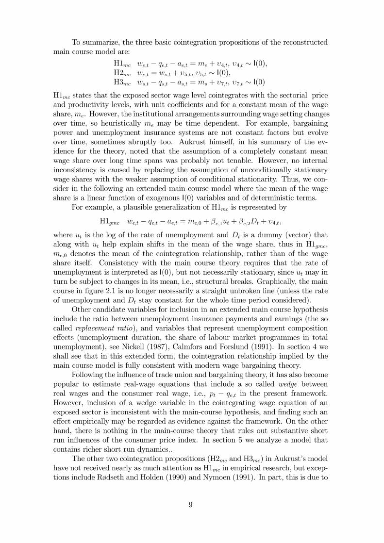
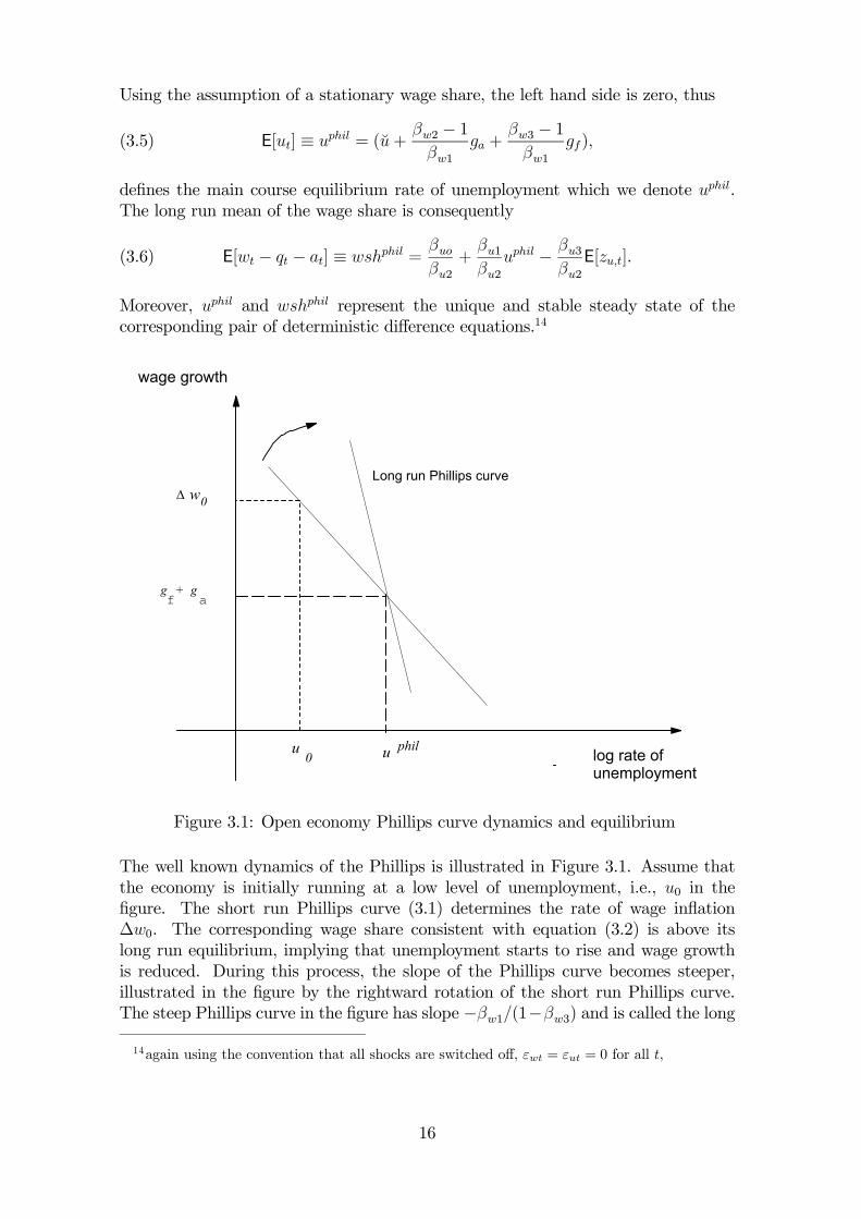
Figure 3.1: Open economy Phillips curve dynamics and equilibrium
The well known dynamics of the Phillips is illustrated in Figure 3.1. Assume thatthe economy is initially running at a low level of unemployment, i.e., u0 in thefigure. The short run Phillips curve (3.1) determines the rate of wage inflation∆w0. The corresponding wage share consistent with equation (3.2) is above itslong run equilibrium, implying that unemployment starts to rise and wage growthis reduced. During this process, the slope of the Phillips curve becomes steeper,illustrated in the figure by the rightward rotation of the short run Phillips curve.The steep Phillips curve in the figure has slope −βw1/(1−βw3) and is called the long14again using the convention that all shocks are switched off, εwt = εut = 0 for all t,
16
run Phillips curve.15 The stable equilibrium is attained when wage growth is equalto the steady state growth of the main-course, i.e., gf + ga and the correspondinglevel of unemployment is given by uphil. The issue about the slope of the long runPhillips curve is seen to hinge on the coefficient βw3, the elasticity of wage growthwith respect to the product price. In the figure, the long run curve is downwardsloping, corresponding to βw3 < 1 which is conventionally referred to as dynamicinhomogeneity in wage setting. The converse, dynamic homogeneity, implies βw3 = 1and a vertical Phillips curve. Subject to dynamic homogeneity, the equilibrium rateumc is independent of world inflation gf .
The slope of the long run Phillips curve represented one of the most debatedissues in macroeconomics in the 1970 and 1980s. One arguments in favour of avertical long run Phillips curve is that workers are able to obtain full compensationfor CPI inflation. Hence βw3 = 1 is reasonable restriction on the Phillips curve,at least if ∆qt is interpreted as an expectations variable. The downward slopinglong run Phillips curve has also been denounced on the grounds that it gives a toooptimistic picture of the powers of economic policy: namely that the government canpermanently reduce the level of unemployment below the natural rate by “fixing” asuitably high level of inflation, see e.g., Romer (1996, Ch 5.5). In the context of anopen economy this discussion appears as somewhat exaggerated, since a long runtrade-off between inflation and unemployment in any case does not follow from thepremise of a downward-sloping long run curve. Instead, as shown in figure 3.1, thesteady state level of unemployment is determined by the rate of imported inflationgf and exogenous productivity growth, ga. Neither of these are normally consideredas instruments (or intermediate targets) of economic policy.16
In the real economy, cost-of-living considerations play an significant role inwage setting, see e.g., Carruth and Oswald (1989, Ch. 3) for a review of industrialrelations evidence. Thus, in applied econometric work, one usually includes currentand lagged CPI-inflation, reflecting the weight put on cost-of-living considerationsin actual wage bargaining situations. To represent that possibility, consider thefollowing system (3.7)-(3.9):
∆wt = βw0 − βw1ut + βw2∆at + βw3∆qt + βw4∆pt + εwt,(3.7)
∆ut = βu0 − βu1ut−1 + βu2(w − q − a)t−1 − βu3zt + εut,(3.8)
∆pt = βp1(∆wt −∆at) + βp2∆qt + εp,t.(3.9)
The first equation augments (3.1) with the change in consumer prices ∆pt, withcoefficient 0 ≤ βw4 ≤ 1. Thus, we have formally other (net) coefficient for the alreadyincluded variables (denoted by the accent above). The second equation is identicalto equation (3.2). The last equation combines the stylized definition of consumerprices in (2.8) with the twin assumption of stationarity of the sheltered sector wages
15By definition, ∆wt = ∆qt +∆at along this curve.16To affect uphil, policy needs to incur a higher or lower permanent rate of currency depreciation.
17
share, and wage leadership of the exposed sector.17 εp,t is the disturbance of thisstochastic price equation.
Using (3.9) to eliminate ∆pt in (3.7) brings us back to (3.1), with coefficientsand εwt suitably redefined. Thus, the expression for the equilibrium rate uphil in (3.5)applies as before. However, it is useful to express uphil in terms of the coefficients ofthe extended system (3.7)-(3.9):
(3.10) uphil = u+βw2 − βw4βp1 − 1
βw1ga +
βw3 + βw4βp2 − 1βw1
gf ,
since this shows that the conventional condition for dynamic homogeneity in wagesetting, βw3+ βw4 = 1, does not imply a vertical long run Phillips curve in this moregeneral case–the required condition is instead βw3 + βw4bp1 = 1, due to the directinfluence of foreign prices on domestic inflation.
In sum, the open economy wage Phillips curve represents one possible speci-fication of the dynamics of the Norwegian model of inflation. Clearly, the dynamicfeatures of our version of the open economy Phillips curve model apply to otherversions of the Phillips curve in that it that implies the natural rate (or a NAIRU)rate of unemployment as a stable stationary solution. It is important to note thatthe Phillips curve needs to be supplemented by an equilibrating mechanism in theform of an equation for the rate of unemployment. Without such an equation inplace, the system is incomplete and we have a missing equation. The question aboutthe dynamic stability of the natural rate (or NAIRU) cannot be addressed in theincomplete Phillips curve system.
Nevertheless, as pointed out by Desai (1995), there is a long standing practiceof basing the estimation of the NAIRU on the incomplete system. For the USA, thequestion of correspondence with a steady state may not be an issue, Staiger et al.(1997) is an example of an important recent study that follows the tradition of esti-mating only the Phillips curve (leaving the equilibrating mechanism, e.g., (3.2) im-plicit). For other countries, European in particular, where the rate of unemploymentappears to be less stationary than in the US, the issue about the correspondencebetween the estimated NAIRUs and the steady state is a more pressing issue.
In the next sections, we turn to two separate aspects of the Phillips curveNAIRU. First, section 3.3 discusses how much flexibility and time dependency onecan allow to enter into NAIRU estimates, while still claiming consistency with thePhillips curve framework. Second, in section 3.4 we discuss the statistical problemsof measuring the uncertainty of an estimated time independent NAIRU.
3.3 Is the Phillips curve consistent with persistent changes in unem-ployment?
In the expressions for the main course NAIRU, (3.5) and (3.10) uphil depends on para-meters of the wage Phillips curve (3.1) and exogenous growth rates. The coefficients
17Hence, the first term in (3.9), reflects normal cost pricing in the sheltered sector, Also, as asimplification, we have imposed identical productivity growth in the two sectors, ∆ae,t = ∆as,t ≡∆at.
18
of the unemployment equation do not enter into the natural rate NAIRU expres-sion. In other version of the Phillips curve, the expression for the NAIRU dependson parameters of price setting as well as wage setting, i.e., the model is specified asa price Phillips curve rather than a wage Phillips curve. But the NAIRU expressionfrom a price Phillips curve remains independent of parameters from equation (3.2)(or its counterpart in other specifications).
The fact that an important system property (the equilibrium of unemploy-ment) can be estimated from a single equation goes some way towards explainingthe popularity of the Phillips curve model. Nevertheless, results based on analysisof the incomplete system give limited information. In particular, a single equationanalysis gives insufficient information of the dynamic properties of the system. First,as we have seen above, unless (3.2) is estimated jointly with the Phillips curve, onecannot show that uphil corresponds to the steady state of the system since the neces-sary and sufficient condition involves the equation for ut, i.e. βu,1 > 0. Thus, singleequation estimates of the NAIRU are subject to the critique that the correspondenceprinciple is violated (see Samuelson (1941)). Second, even if one is convinced apriorithat uphil corresponds to the steady state of the system, the speed of adjustmenttowards the steady state is clearly of interest and requires estimation of equation(3.2) as well as of the Phillips curve (3.1).
During the last 20-25 years of the previous century, European rates of unem-ployment rose sharply and showed no sign of reverting to the levels of the 1960s and1970s. Understanding of the stubbornly high unemployment called for models that,i) allow for long adjustments lags around a constant natural rate, or ii), the modelmust allow the equilibrium to change. A combination of the two are of course alsopossible.
Simply by virtue of being a dynamic system, the Phillips curve model accom-modates slow dynamics. In principle, the adjustment coefficient βu1 in the unem-ployment equation (3.2) can be arbitrarily small–as long as it is not zero the uphil
formally corresponds to the steady state of the system. However, there is a questionof how just slow the speed of adjustment can be before the concept of equilibriumis undermined “from within”. Put differently, the essence of the Phelps/Friedmanargument was that is that the natural rate was quite stable and that it is strong at-tractor of the actual rate of unemployment (i.e., βu1 is not numerically significant),see Phelps (1995). However, the experience of the 1980s and 1990s have learnt usthat the natural rate is at best a weak attractor. There are important practicalaspects of this issue too: Policy makers, pondering the prospects after a negativeshock to the economy, will find small comfort in learning that eventually the rateof unemployment will return to its natural rate, but only after 40 years or more!In section 3.6 we show how this kind of internal inconsistency arise in an otherwisequite respectable empirical version of the Phillips curve system (3.1)- (3.2).
Moreover, the Phillips curve framework offers only limited scope for an eco-nomic explanation of the regime shifts that some time occur in the mean of therate of unemployment. True, expression (3.10) contains a long-run Okun’s law typerelationship between the rate of unemployment and the rate of productivity growth.However, it seems somewhat incredible that changes in the real growth rate δa aloneshould account for the sharp and persistent rises in the rate of unemployment expe-rienced in Europe. A nominal growth rate like δf can of course undergo sharp and
19
large rises, but for those changes to have an impact on the equilibrium rate requiresa downward sloping long run Phillips curve–which many macroeconomists will notaccept.
Thus, the Phillips curve is better adapted to a stable regime characterized bya modest adjustment lag around a fairly stable mean rate of unemployment, thanto the regime shift in European unemployment of the 1980s and 1990s. This is thebackground against which the appearance of new models in the 1980s must be seen,i.e., models that promised to be able to explain the shifts in the equilibrium rateof unemployment, see Backhouse (2000), and there is now a range of specificationsof how the “structural characteristic of labour and commodity markets” affects theequilibrium paths of unemployment, see Nickell (1993) for a survey and section 4of this book. Arguably however, none of the new models have reached the statusof being an undisputed consensus model that was once was the role of the Phillipscurve.
So far we have discussed permanent changes in unemployment as being due tolarge deterministic shifts that occur intermittently, in line with our maintained viewof the rate of unemployment as I(0) but subject to (infrequent) structural breaks.An alternative view, which has become influential in the USA, is the so called timevarying NAIRU, cf. Gordon (1997) and Staiger et al. (1997). The basic idea is thatthe NAIRU reacts to small supply side shocks that occur frequently. The followingmodifications of equation (3.3) defines the time varying NAIRU
∆wt = −βw1(ut − ut) + βw2∆at + βw3∆qt + εwt,(3.11)
ut = ut−1 + εu,t.(3.12)
The telling difference is that the natural rate u is no longer a time independentparameter, but a stochastic parameter that follows the random walk (3.12), anda disturbance εu,t which in this model represents small supply side shocks. Whenestimating this pair of equations (by the Kalman filter) the standard error of εu,tneeds to be limited in the outset, otherwise ut will jump up and down and soakup all the variation in ∆wt left unexplained by the conventional explanatory vari-ables. Hence, time varying NAIRU estimates tend to reflect how much variability aresearcher accepts and finds possible to communicate to the community. Logically,the methodology implies a unit root, both in the observed rate of unemploymentand in the NAIRU itself. Finally, the practical relevance of this framework seemsto be limited to the USA, where there are few big and lasting shifts in the rate ofunemployment.
Related to the time varying NAIRU is the concept of hysteresis. FollowingBlanchard and Summers (1986), economists invoked the term unemployment ‘hys-teresis’ for the case of a unit root in the rate of unemployment, in which case theequilibrium rate might be said to become identical to the lagged rate of unemploy-ment. However, Røed (1994) instructively draws the distinction between genuinehysteresis as a non-linear and multiple equilibrium phenomenon, and the linearproperty of a unit root. Moreover, Cross (1995) have shown convincingly shownthat ‘hysteresis’ is not actually hysteresis (in its true meaning, as a non-linear phe-nomenon), and that proper hysteresis creates a time path for unemployment whichis inconsistent with the natural rate hypothesis.
20
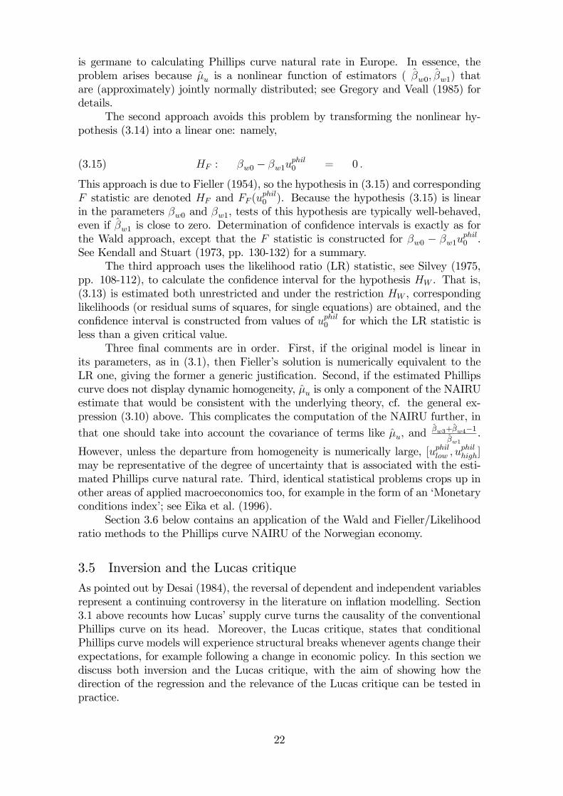
3.4 Estimating the uncertainty of the Phillips curve NAIRUThis subsection describes three approaches for estimation of a ‘confidence region’of a (time independent) Phillips curve NAIRU. As noted by Staiger et al. (1997)the reason for the absence of confidence intervals in most NAIRU calculations hasto do with the fact that the NAIRU (e.g., in (3.4) is a non-linear function of theregression coefficients. Nevertheless, three approaches can be used to used to con-struct confidence intervals for the NAIRU: the Wald, Fieller, and likelihood ratiostatistics.18 The Fieller and likelihood ratio forms appear preferable because of theirfinite sample properties.
The first and most intuitive approach is based on the associated standard errorand t ratio for the estimated coefficients, and thus corresponds to a Wald statistic;see Wald (1943) and Silvey (1975, pp. 115-118). This method may be characterizedas follows. A wage Phillips curve is estimated in the form of (3.1) in section 3.2. Inthe case of full pass-through of productivity gains on wages, and no ‘money illusion”,the Phillips curve NAIRU uphil is βw0/βw1, and its estimated value µu is βw0/βw1,where a circumflex denotes estimated values. As already noted (3.1) is convenientlyrewritten as:
(3.13) ∆wt −∆at −∆qt = −βw1(ut − uphil) + εwt.
where uphil may be estimated directly by (say) non-linear least squares. The resultis numerically equivalent to the ratio βw0/βw1 derived from the linear estimates(βw0, βw1) in (3.1). In either case, a standard error for µ
phil can be computed, fromwhich confidence intervals are directly obtained.
More generally, a confidence interval includes the unconstrained/most likelyestimate of uphil, which is βw0/βw1, and some region around that value. Heuristically,the confidence interval contains each value of the ratio that does not violate thehypothesis
(3.14) HW : βw0/βw1 = uphil0
too strongly in the data. More formally, let FW (uphil0 ) be the Wald-based F statistic
for testing HW , and let Pr(·) be the probability of its argument. Then, a confidenceinterval of (1 − α)% is [uphillow , u
philhigh] defined by Pr(FW (u
phil0 )) ≤ 1 − α for uphil0 ∈
[uphillow , uphilhigh].If βw1, the elasticity of the rate of unemployment in the Phillips curve, is
precisely estimated, the Wald approach is usually quite satisfactory. Small samplesizes clearly endangers estimation precision, but “how small is small” depends on theamount of information “per observation” and the effective sample size. However,if βw1 is imprecisely estimated (i.e., not very significant statistically), then thisapproach can be highly misleading. Specifically, the Wald approach ignores howβw0/βw1 behaves for values of βw1 relatively close to zero, where “relatively” reflectsthe uncertainty in the estimate of βw1. As explained above, for European Phillipscurves, the βw1 estimates are typically insignificant statistically, so this concern
18This paragraph draws on Ericsson et al. (1997).
21
is germane to calculating Phillips curve natural rate in Europe. In essence, theproblem arises because µu is a nonlinear function of estimators ( βw0, βw1) thatare (approximately) jointly normally distributed; see Gregory and Veall (1985) fordetails.
The second approach avoids this problem by transforming the nonlinear hy-pothesis (3.14) into a linear one: namely,
(3.15) HF : βw0 − βw1uphil0 = 0 .
This approach is due to Fieller (1954), so the hypothesis in (3.15) and correspondingF statistic are denoted HF and FF (u
phil0 ). Because the hypothesis (3.15) is linear
in the parameters βw0 and βw1, tests of this hypothesis are typically well-behaved,even if βw1 is close to zero. Determination of confidence intervals is exactly as forthe Wald approach, except that the F statistic is constructed for βw0 − βw1u
phil0 .
See Kendall and Stuart (1973, pp. 130-132) for a summary.The third approach uses the likelihood ratio (LR) statistic, see Silvey (1975,
pp. 108-112), to calculate the confidence interval for the hypothesis HW . That is,(3.13) is estimated both unrestricted and under the restriction HW , correspondinglikelihoods (or residual sums of squares, for single equations) are obtained, and theconfidence interval is constructed from values of uphil0 for which the LR statistic isless than a given critical value.
Three final comments are in order. First, if the original model is linear inits parameters, as in (3.1), then Fieller’s solution is numerically equivalent to theLR one, giving the former a generic justification. Second, if the estimated Phillipscurve does not display dynamic homogeneity, µu is only a component of the NAIRUestimate that would be consistent with the underlying theory, cf. the general ex-pression (3.10) above. This complicates the computation of the NAIRU further, in
that one should take into account the covariance of terms like µu, andβw3+βw4−1
βw1.
However, unless the departure from homogeneity is numerically large, [uphillow , uphilhigh]
may be representative of the degree of uncertainty that is associated with the esti-mated Phillips curve natural rate. Third, identical statistical problems crops up inother areas of applied macroeconomics too, for example in the form of an ‘Monetaryconditions index’; see Eika et al. (1996).
Section 3.6 below contains an application of the Wald and Fieller/Likelihoodratio methods to the Phillips curve NAIRU of the Norwegian economy.
3.5 Inversion and the Lucas critiqueAs pointed out by Desai (1984), the reversal of dependent and independent variablesrepresent a continuing controversy in the literature on inflation modelling. Section3.1 above recounts how Lucas’ supply curve turns the causality of the conventionalPhillips curve on its head. Moreover, the Lucas critique, states that conditionalPhillips curve models will experience structural breaks whenever agents change theirexpectations, for example following a change in economic policy. In this section wediscuss both inversion and the Lucas critique, with the aim of showing how thedirection of the regression and the relevance of the Lucas critique can be tested inpractice.
22
3.5.1 Inversion
Under super-exogeneity, the results for an conditional econometric model, e.g., aconventional augmented Phillips curve, is not invariant to a re-normalization. Oneway to see this is to invoke the well known formulae
(3.16) β · β0= r2yx
where ryx denotes the correlation coefficient and β is the estimated regression coef-
ficient when y is the dependent variable and x is the regressor. β0is the estimated
coefficient in the reverse regression. By definition, ‘regime shifts’ entail that corre-lation structures alter, hence ryx shifts. If, due to super exogeneity, β nevertheless
is constant, then β0cannot be constant.
(3.16) generalizes directly, with ryx interpreted as the partial correlation co-efficient. Hence, if for example the Phillips curve (3.1) is estimated by OLS, thenfinding that βw1 is recursively stable entails that β
0w1 for the re-normalized equation
(on the rate of unemployment) is recursively unstable. Thus finding a stable Phillipscurve over a sample period that contains changes in the (partial) correlations, re-futes that the model has a Lucas supply curve interpretation. This simple procedurealso applies to estimation by instrumental variables (due to endogeneity of e.g., ∆qtand/or ∆pt) provided that the number of instrumental variables is greater than thenumber of endogenous variables in the Phillips curve.
3.5.2 Lucas critique
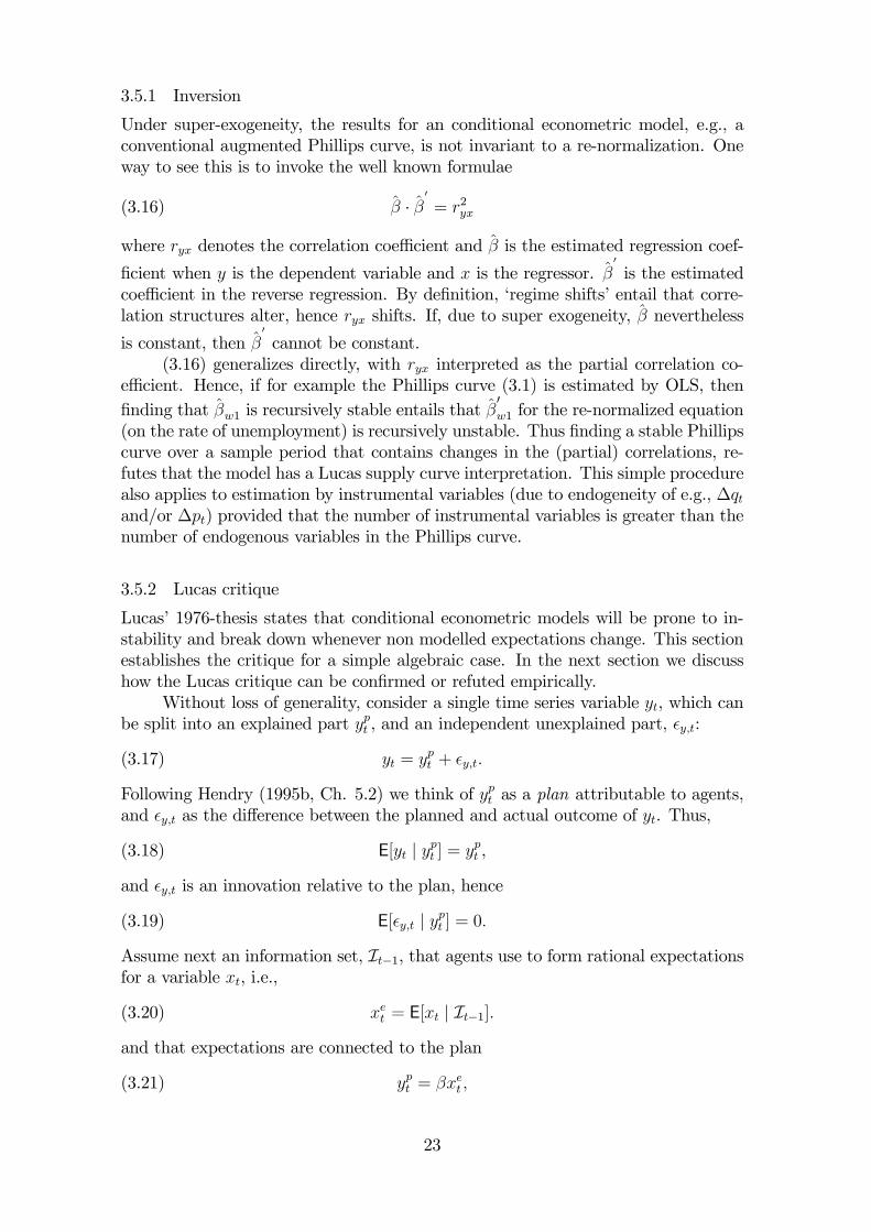
Lucas’ 1976-thesis states that conditional econometric models will be prone to in-stability and break down whenever non modelled expectations change. This sectionestablishes the critique for a simple algebraic case. In the next section we discusshow the Lucas critique can be confirmed or refuted empirically.
Without loss of generality, consider a single time series variable yt, which canbe split into an explained part ypt , and an independent unexplained part, y,t:
(3.17) yt = ypt + y,t.
Following Hendry (1995b, Ch. 5.2) we think of ypt as a plan attributable to agents,and y,t as the difference between the planned and actual outcome of yt. Thus,
(3.18) E[yt | ypt ] = ypt ,
and y,t is an innovation relative to the plan, hence
(3.19) E[ y,t | ypt ] = 0.Assume next an information set, It−1, that agents use to form rational expectationsfor a variable xt, i.e.,
(3.20) xet = E[xt | It−1].and that expectations are connected to the plan
(3.21) ypt = βxet ,
23

which is usually motivated by, or derived from, economic theory.By construction, E[ypt | It−1] = ypt , while we assume that y,t in (3.17) is an
innovation
(3.22) E[ y,t | It−1] = 0,and, therefore
(3.23) E[yt | It−1] = ypt .
Initially, xet is assumed to follow a first order AR process (non stationarity is con-sidered below):
(3.24) xet = E[xt | It−1] = α1xt−1, |α1| < 1.Thus xt = xet + x,t, or:
(3.25) xt = α1xt−1 + x,t, E[ x,t | xt−1] = 0,For simplicity, we assume that y,t and x,t are independent.
Assume next that the single parameter of interest is β in equation (3.21). Thereduced form of yt follows from (3.17), (3.21) and (3.24):
(3.26) yt = α1βxt−1 + x,t,
where xt is weakly exogenous for ξ = α1β, but the parameter of interest β is notidentifiable from (3.26) alone. Moreover the reduced form equation (3.26), whileallowing us to estimate ξ consistently in a state of nature characterized by station-arity, is susceptible to the Lucas critique, since ξ is not invariant to changes in theautoregressive parameter of the marginal model (3.24).
In practice, the Lucas critique is usually aimed at ‘behavioural equations’ insimultaneous equations systems, for example
(3.27) yt = βxt + ηt,
with disturbance term:
(3.28) ηt = y,t − x,tβ.
It is straight forward (see appendix A) to show that estimation of (3.27) by OLS ona sample t = 1, 2, ..T , gives
(3.29) plimT→∞
βOLS = α21β,
showing that, ‘regressing yt on xt’ does not represent the counterpart to ypt = xetβ in
(3.21). Specifically, instead of β, we estimate α21β, and changes in the expectationparameter α1 damages the stability of the estimates, thus confirming the Lucascritique.
However, the applicability of the critique rests on the assumptions made. Forexample, if we change the assumption of |α1| < 1 to α1 = 1, so that xt has aunit root but is cointegrated with yt, the Lucas critique does not apply: Under
24
cointegration, plimT→∞1 βOLS = β , since the cointegration parameter is unique andcan be estimated consistently by OLS.
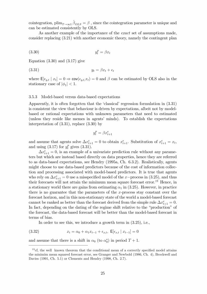
As another example of the importance of the exact set of assumptions made,consider replacing (3.21) with another economic theory, namely the contingent plan
(3.30) ypt = βxt
Equation (3.30) and (3.17) give
(3.31) yt = βxt + t
where E[ y,t | xt] = 0⇒ cov( y,t,xt) = 0 and β can be estimated by OLS also in thestationary case of |φ1| < 1.
3.5.3 Model-based versus data-based expectations
Apparently, it is often forgotten that the ‘classical’ regression formulation in (3.31)is consistent the view that behaviour is driven by expectations, albeit not by model-based or rational expectations with unknown parameters that need to estimated(unless they reside like memes in agents’ minds). To establish the expectationsinterpretation of (3.31), replace (3.30) by
ypt = βxet+1
and assume that agents solve ∆xet+1 = 0 to obtain xet+1. Substitution of xet+1 = xt,
and using (3.17) for ypt gives (3.31).∆xet+1 = 0, is an example of a univariate prediction rule without any parame-
ters but which are instead based directly on data properties, hence they are referredto as data-based expectations, see Hendry (1995a, Ch. 6.3.2). Realistically, agentsmight choose to use data-based predictors because of the cost of information collec-tion and processing associated with model-based predictors. It is true that agentswho rely on ∆xet+1 = 0 use a misspecified model of the x−process in (3.25), and thustheir forecasts will not attain the minimum mean square forecast error.19 Hence, ina stationary world there are gains from estimating α1 in (3.25). However, in practicethere is no guarantee that the parameters of the x-process stay constant over theforecast horizon, and in this non-stationary state of the world a model-based forecastcannot be ranked as better than the forecast derived from the simple rule∆xet+1 = 0.In fact, depending on the dating of the regime shift relative to the “production” ofthe forecast, the data-based forecast will be better than the model-based forecast interms of bias.
In order to see this, we introduce a growth term in (3.25), i.e.,
(3.32) xt = α0 + α1xt−1 + x,t, E[ x,t | xt−1] = 0and assume that there is a shift in α0 (to α∗0) in period T + 1.
19cf, the well known theorem that the conditional mean of a correctly specified model attainsthe minimim mean squared forecast error, see Granger and Newbold (1986, Ch. 4), Brockwell andDavies (1991, Ch. 5.1) or Clements and Hendry (1998, Ch. 2.7).
25
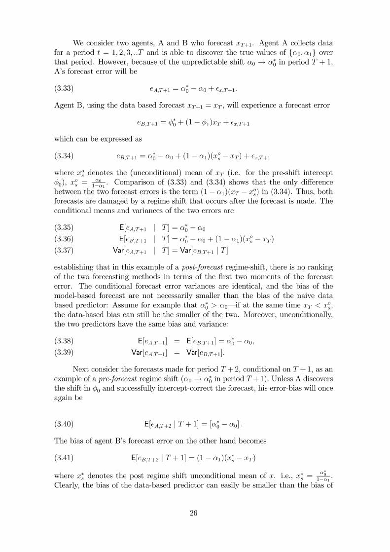
We consider two agents, A and B who forecast xT+1. Agent A collects datafor a period t = 1, 2, 3, ..T and is able to discover the true values of {α0, α1} overthat period. However, because of the unpredictable shift α0 → α∗0 in period T + 1,A’s forecast error will be
(3.33) eA,T+1 = α∗0 − α0 + x,T+1.
Agent B, using the data based forecast xT+1 = xT , will experience a forecast error
eB,T+1 = φ∗0 + (1− φ1)xT + x,T+1
which can be expressed as
(3.34) eB,T+1 = α∗0 − α0 + (1− α1)(xos − xT ) + x,T+1
where xos denotes the (unconditional) mean of xT (i.e. for the pre-shift interceptφ0), x
os =
α01−α1 . Comparison of (3.33) and (3.34) shows that the only difference
between the two forecast errors is the term (1− α1)(xT − xos) in (3.34). Thus, bothforecasts are damaged by a regime shift that occurs after the forecast is made. Theconditional means and variances of the two errors are
E[eA,T+1 | T ] = α∗0 − α0(3.35)
E[eB,T+1 | T ] = α∗0 − α0 + (1− α1)(xos − xT )(3.36)
Var[eA,T+1 | T ] = Var[eB,T+1 | T ](3.37)
establishing that in this example of a post-forecast regime-shift, there is no rankingof the two forecasting methods in terms of the first two moments of the forecasterror. The conditional forecast error variances are identical, and the bias of themodel-based forecast are not necessarily smaller than the bias of the naive databased predictor: Assume for example that α∗0 > α0–if at the same time xT < xos,the data-based bias can still be the smaller of the two. Moreover, unconditionally,the two predictors have the same bias and variance:
E[eA,T+1] = E[eB,T+1] = α∗0 − α0,(3.38)
Var[eA,T+1] = Var[eB,T+1].(3.39)
Next consider the forecasts made for period T +2, conditional on T +1, as anexample of a pre-forecast regime shift (α0 → α∗0 in period T +1). Unless A discoversthe shift in φ0 and successfully intercept-correct the forecast, his error-bias will onceagain be
(3.40) E[eA,T+2 | T + 1] = [α∗0 − α0] .
The bias of agent B’s forecast error on the other hand becomes
(3.41) E[eB,T+2 | T + 1] = (1− α1)(x∗s − xT )
where x∗s denotes the post regime shift unconditional mean of x. i.e., x∗s =
α∗01−α1 .
Clearly, the bias of the data-based predictor can easily be smaller than the bias of
26
the model-based prediction error (but the opposite can of course also be the case).However,
E[eA,T+2] = [α∗0 − α0] ,
E[eB,T+2] = 0
and the unconditional forecast errors are always smallest for the data-based predic-tion in this case of pre-forecast regime shift.
The analysis generalizes to the case of a unit root in the x-process, in fact itis seen directly from the above that the data-based forecast errors have even betterproperties for the case of α1 = 1, e.g., E[eB,T+2 | T + 1] = 0 in (3.41). Moregenerally, if xt is I(d), then solving ∆dxet+1 = 0 to obtain xet+1 will result in forecastwith the same robustness with respect to regime shifts as illustrated in our example,see Hendry (1995a, Ch.6.2.3). This class of predictors belong to forecasting modelsthat are cast in terms of differences of the original data, i.e., differenced vectorautoregressions, denoted dVARs. They have a tradition in macroeconomics that atleast goes back to the 1970s, then in the form of Box-Jenkins time series analysis andARIMA models. A common tread running trough many published evaluations offorecasts, is that the naive time series forecasts are often superior to the forecasts ofthe macroeconometric models under scrutiny, see e.g. Granger and Newbold (1986,Ch. 9.4). Why dVARs tend to do so well in forecast competitions is now understoodmore fully, thanks to the work of e.g., Clements and Hendry (1996,1998 ,1999). Inbrief, the explanation is exactly along the lines of our comparison of ‘naive’ and‘sophisticated’ expectation formation above: The dVAR provides robust forecastsof non stationary time series are subject to intermittent regime shifts. To beatthem, the user of an econometric models must regularly take recourse to interceptcorrections and other judgemental corrections, see section XX below.
3.5.4 Testing the Lucas critique
While it is logically possible that conventional Phillips curves are ‘really’ Lucassupply functions in reverse, that claim can be tested for specific models. Findingthat the Phillips curve is stable over sample periods that included regime shifts andchanges in the correlation structures is sufficient for refuting inversion. Likewise, theLucas critique is a possibility theorem, not a truism, see Ericsson and Irons (1995),and its assumptions have testable implications. For example, the Lucas critiqueimplies i) that βOLS is non constant as α1 changes (inside the unit circle), and ii)that determinants of α1 (if identifiable in practice) should affect βOLS if includedin the conditional model of yt. Conversely, the Lucas critique is inconsistent withthe joint finding of a stable conditional relationship and a regime shift occurring inthe process which drives the explanatory variable, see Ericsson and Hendry (1999).Based on this logic methods of testing the Lucas critique have been developed, seee.g., Hendry (1988), Engle and Hendry (1993), and Favero and Hendry (1992).
Two surveys of the empirical evidence for the Lucas critique are found inEricsson and Irons (1995) and Stanley (2000). Though very different in methodology,the two studies conclude in a similar fashion, namely that there is little firm evidencesupporting the empirical applicability of the Lucas critique. In the next section 3.6we review the applicability of the Lucas critique to the Norwegian Phillips curve.
27
As an alternative to rational expectations, we note as a possibility that agents formexpectations on the basis of observed properties of the data itself. Interestingly,there is a close relationship between data-based forecasting rules that agents maypick up, and the times series models that have been successful in macroeconomicforecasting.
3.6 An empirical open economy Phillips curve systemIn this section we first specify and then evaluate an open economy Phillips curve forthe Norwegian manufacturing sector. We use an annual data set for the period 1965-1998, which is used again in later sections where competing models are estimated. Inthe choice of explanatory variables and of data transformations, we build on existingstudies of the Phillips curve in Norway, cf. Stølen (1990,1993). The variables are inlog scale (unless otherwise stated) and are defined as follows (appendix C.1 containsmore details):
wct = hourly wage cost in manufacturing;
qt = index of producer prices (value added deflator);
pt = the official consumer price index;
at = average labour productivity;
tut = rate of total unemployment (i.e., unemployment includes participants inactive labour market programmes);
rprt = the replacement ratio;
h = the length of the “normal" working day in manufacturing;
t1 = the manufacturing industry payroll tax-rate (not log).
Equation (3.42) shows the estimation results of a manufacturing sector Phillipscurve which is as general as the number of observations allows.20 Arguably the use ofordinary least squares estimation (OLS) may be defended by invoking main-coursetheory (remembering that we model wages of an exposed industry), but the mainreason here is plain simplicity, and we return to the estimation of the Phillips curveby system methods below.
The model is a straight forward application of the theoretical Phillips curve in(3.1): We include two lags in ∆qt and ∆at, and, as discussed above, it is a necessaryconcession to realism to also include a lag polynomial of the consumer price inflationrate, ∆pt. We use only one lag of the unemployment rate, since previous work onthis data set gives no indication of any need to include a second lag of this variable.
20Batch files: aar_NmcPhil.fl (PcGive) and aar_NmcPhil_gets.fl (PcGets).
28
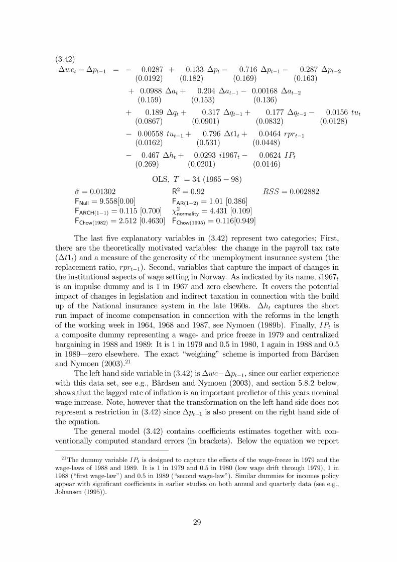
∆wct −∆pt−1 = − 0.0287(0.0192)
+ 0.133(0.182)
∆pt − 0.716(0.169)
∆pt−1 − 0.287(0.163)
∆pt−2
+ 0.0988(0.159)
∆at + 0.204(0.153)
∆at−1 − 0.00168(0.136)
∆at−2
+ 0.189(0.0867)
∆qt + 0.317(0.0901)
∆qt−1 + 0.177(0.0832)
∆qt−2 − 0.0156(0.0128)
tut
− 0.00558(0.0162)
tut−1 + 0.796(0.531)
∆t1t + 0.0464(0.0448)
rprt−1
− 0.467(0.269)
∆ht + 0.0293(0.0201)
i1967t − 0.0624(0.0146)
IPt
(3.42)
OLS, T = 34 (1965− 98)σ = 0.01302 R2 = 0.92 RSS = 0.002882FNull = 9.558[0.00] FAR(1−2) = 1.01 [0.386]FARCH(1−1) = 0.115 [0.700] χ2normality = 4.431 [0.109]FChow(1982) = 2.512 [0.4630] FChow(1995) = 0.116[0.949]
The last five explanatory variables in (3.42) represent two categories; First,there are the theoretically motivated variables: the change in the payroll tax rate(∆t1t) and a measure of the generosity of the unemployment insurance system (thereplacement ratio, rprt−1). Second, variables that capture the impact of changes inthe institutional aspects of wage setting in Norway. As indicated by its name, i1967tis an impulse dummy and is 1 in 1967 and zero elsewhere. It covers the potentialimpact of changes in legislation and indirect taxation in connection with the buildup of the National insurance system in the late 1960s. ∆ht captures the shortrun impact of income compensation in connection with the reforms in the lengthof the working week in 1964, 1968 and 1987, see Nymoen (1989b). Finally, IPt isa composite dummy representing a wage- and price freeze in 1979 and centralizedbargaining in 1988 and 1989: It is 1 in 1979 and 0.5 in 1980, 1 again in 1988 and 0.5in 1989–zero elsewhere. The exact “weighing” scheme is imported from Bårdsenand Nymoen (2003).21
The left hand side variable in (3.42) is∆wc−∆pt−1, since our earlier experiencewith this data set, see e.g., Bårdsen and Nymoen (2003), and section 5.8.2 below,shows that the lagged rate of inflation is an important predictor of this years nominalwage increase. Note, however that the transformation on the left hand side does notrepresent a restriction in (3.42) since ∆pt−1 is also present on the right hand side ofthe equation.
The general model (3.42) contains coefficients estimates together with con-ventionally computed standard errors (in brackets). Below the equation we report
21The dummy variable IPt is designed to capture the effects of the wage-freeze in 1979 and thewage-laws of 1988 and 1989. It is 1 in 1979 and 0.5 in 1980 (low wage drift through 1979), 1 in1988 (“first wage-law”) and 0.5 in 1989 (“second wage-law”). Similar dummies for incomes policyappear with significant coefficients in earlier studies on both annual and quarterly data (see e.g.,Johansen (1995)).
29
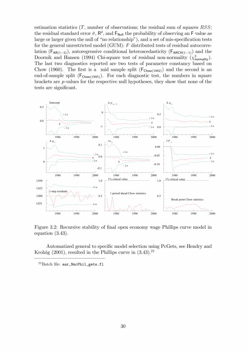
estimation statistics (T , number of observations; the residual sum of squares RSS;the residual standard error σ, R2, and FNull the probability of observing an F value aslarge or larger given the null of “no relationship”), and a set of mis-specification testsfor the general unrestricted model (GUM): F distributed tests of residual autocorre-lation (FAR(1−2)), autoregressive conditional heteroscedasticity (FARCH(1−1)) and theDoornik and Hansen (1994) Chi-square test of residual non-normality (χ2normality).The last two diagnostics reported are two tests of parameter constancy based onChow (1960). The first is a mid sample split (FChow(1982)) and the second is anend-of-sample split (FChow(1995)). For each diagnostic test, the numbers in squarebrackets are p-values for the respective null hypotheses, they show that none of thetests are significant.
1980 1990 2000
0.0
0.5
β
+ 2 σ
− 2 σ
Intercept
1980 1990 2000
-1
0
− 2 σ
β
+ 2 σ
∆ p t − 1
1980 1990 2000
0.0
0.5
β
+ 2 σ
− 2 σ
∆ q t
1980 1990 2000
0
1
+ 2 σβ− 2 σ
∆ q t
1980 1990 2000
-0.1
0.0
0.1
+ 2 σ
β
− 2 σ
t u t
1980 1990 2000
-0.10
-0.05
0.00
+ 2 σ
− 2 σβ
I P t
1980 1990 2000
0.025
0.000
0.025
0.050
+2 se
-2 se
1-step residuals
1980 1990 2000
0.5
1.0
1 period ahead Chow statistics
1% critical value
1980 1990 2000
0.5
1.0 1% critical value
Break point Chow statistics
Figure 3.2: Recursive stability of final open economy wage Phillips curve model inequation (3.43).
Automatized general to specific model selection using PcGets, see Hendry andKrolzig (2001), resulted in the Phillips curve in (3.43).22
22Batch file: aar_NmcPhil_gets.fl
30
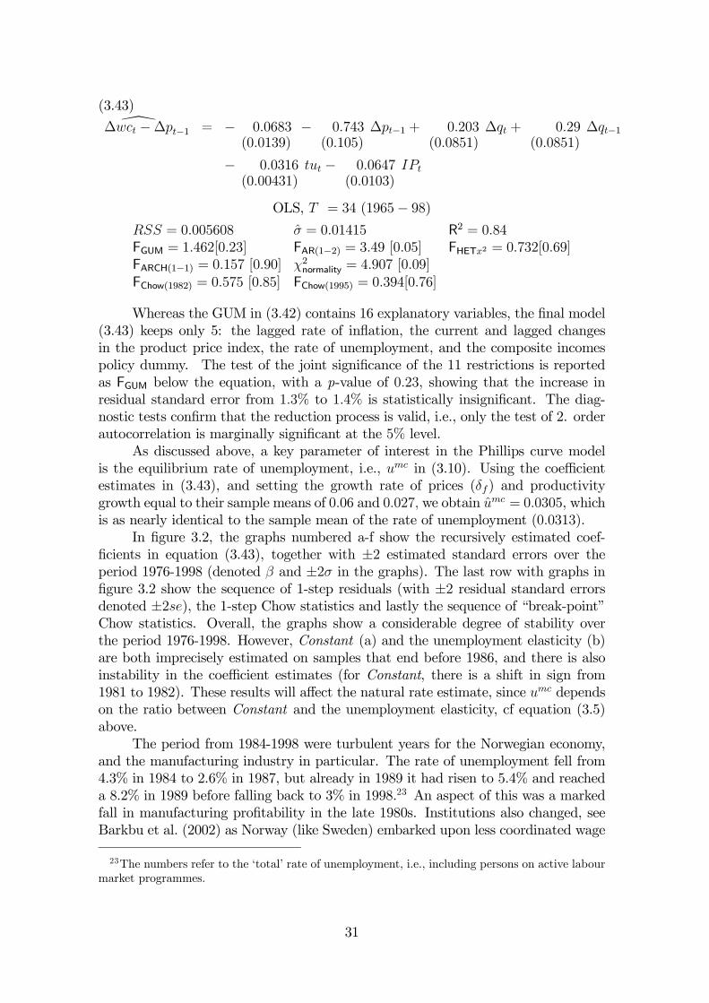
\∆wct −∆pt−1 = − 0.0683(0.0139)
− 0.743(0.105)
∆pt−1 + 0.203(0.0851)
∆qt + 0.29(0.0851)
∆qt−1
− 0.0316(0.00431)
tut − 0.0647(0.0103)
IPt
(3.43)
OLS, T = 34 (1965− 98)RSS = 0.005608 σ = 0.01415 R2 = 0.84FGUM = 1.462[0.23] FAR(1−2) = 3.49 [0.05] FHETx2 = 0.732[0.69]FARCH(1−1) = 0.157 [0.90] χ2normality = 4.907 [0.09]FChow(1982) = 0.575 [0.85] FChow(1995) = 0.394[0.76]
Whereas the GUM in (3.42) contains 16 explanatory variables, the final model(3.43) keeps only 5: the lagged rate of inflation, the current and lagged changesin the product price index, the rate of unemployment, and the composite incomespolicy dummy. The test of the joint significance of the 11 restrictions is reportedas FGUM below the equation, with a p-value of 0.23, showing that the increase inresidual standard error from 1.3% to 1.4% is statistically insignificant. The diag-nostic tests confirm that the reduction process is valid, i.e., only the test of 2. orderautocorrelation is marginally significant at the 5% level.
As discussed above, a key parameter of interest in the Phillips curve modelis the equilibrium rate of unemployment, i.e., umc in (3.10). Using the coefficientestimates in (3.43), and setting the growth rate of prices (δf) and productivitygrowth equal to their sample means of 0.06 and 0.027, we obtain umc = 0.0305, whichis as nearly identical to the sample mean of the rate of unemployment (0.0313).
In figure 3.2, the graphs numbered a-f show the recursively estimated coef-ficients in equation (3.43), together with ±2 estimated standard errors over theperiod 1976-1998 (denoted β and ±2σ in the graphs). The last row with graphs infigure 3.2 show the sequence of 1-step residuals (with ±2 residual standard errorsdenoted ±2se), the 1-step Chow statistics and lastly the sequence of “break-point”Chow statistics. Overall, the graphs show a considerable degree of stability overthe period 1976-1998. However, Constant (a) and the unemployment elasticity (b)are both imprecisely estimated on samples that end before 1986, and there is alsoinstability in the coefficient estimates (for Constant, there is a shift in sign from1981 to 1982). These results will affect the natural rate estimate, since umc dependson the ratio between Constant and the unemployment elasticity, cf equation (3.5)above.
The period from 1984-1998 were turbulent years for the Norwegian economy,and the manufacturing industry in particular. The rate of unemployment fell from4.3% in 1984 to 2.6% in 1987, but already in 1989 it had risen to 5.4% and reacheda 8.2% in 1989 before falling back to 3% in 1998.23 An aspect of this was a markedfall in manufacturing profitability in the late 1980s. Institutions also changed, seeBarkbu et al. (2002) as Norway (like Sweden) embarked upon less coordinated wage
23The numbers refer to the ‘total’ rate of unemployment, i.e., including persons on active labourmarket programmes.
31
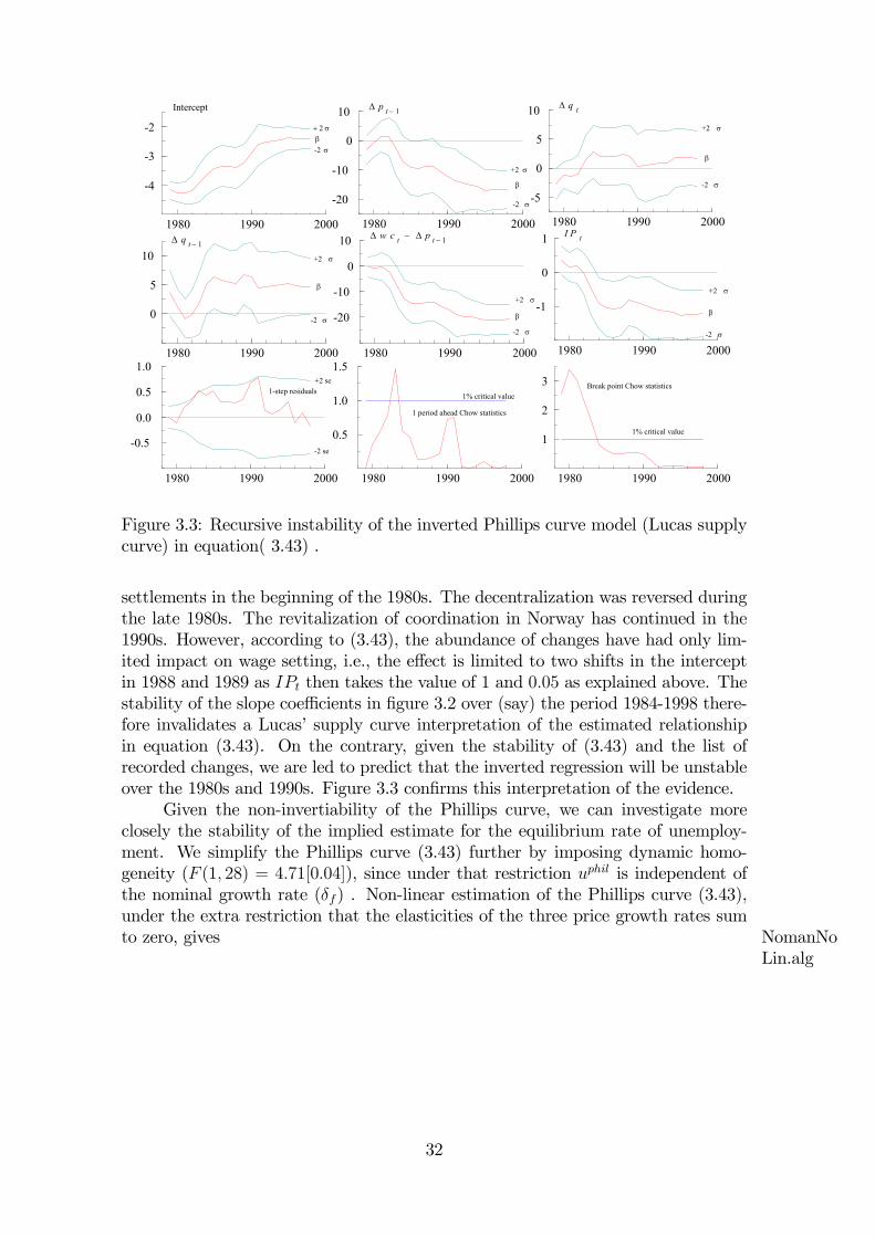
1980 1990 2000
-20
-10
0
10
+2 σ
+2 σ
-2 σ
β
∆ w c t − ∆ p t − 1
1980 1990 2000
-4
-3
-2 + 2 σβ-2 σ
Intercept
1980 1990 2000
-20
-10
0
10
+2 σ
β
-2 σ
∆ p t − 1
1980 1990 2000
-5
0
5
10
-2 σ
β
∆ q t
1980 1990 2000
0
5
10
-2 σ
+2 σ
β
∆ q t − 1
1980 1990 2000
-1
0
1
+2 σ
-2 σ
β
I P t
1980 1990 2000
-0.5
0.0
0.5
1.0+2 se
-2 se
1-step residuals
1980 1990 2000
0.5
1.0
1.5
1% critical value
1980 1990 2000
1
2
3
1 period ahead Chow statistics
1% critical value
Break point Chow statistics
Figure 3.3: Recursive instability of the inverted Phillips curve model (Lucas supplycurve) in equation( 3.43) .
settlements in the beginning of the 1980s. The decentralization was reversed duringthe late 1980s. The revitalization of coordination in Norway has continued in the1990s. However, according to (3.43), the abundance of changes have had only lim-ited impact on wage setting, i.e., the effect is limited to two shifts in the interceptin 1988 and 1989 as IPt then takes the value of 1 and 0.05 as explained above. Thestability of the slope coefficients in figure 3.2 over (say) the period 1984-1998 there-fore invalidates a Lucas’ supply curve interpretation of the estimated relationshipin equation (3.43). On the contrary, given the stability of (3.43) and the list ofrecorded changes, we are led to predict that the inverted regression will be unstableover the 1980s and 1990s. Figure 3.3 confirms this interpretation of the evidence.
Given the non-invertiability of the Phillips curve, we can investigate moreclosely the stability of the implied estimate for the equilibrium rate of unemploy-ment. We simplify the Phillips curve (3.43) further by imposing dynamic homo-geneity (F (1, 28) = 4.71[0.04]), since under that restriction uphil is independent ofthe nominal growth rate (δf) . Non-linear estimation of the Phillips curve (3.43),under the extra restriction that the elasticities of the three price growth rates sumto zero, gives NomanNo
Lin.alg
32
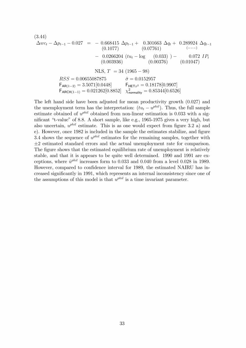
∆wct −∆pt−1 − 0.027 = − 0.668415(0.1077)
∆pt−1 + 0.301663(0.07761)
∆qt + 0.289924(−−−)
∆qt−1
− 0.0266204(0.003936)
(tut − log (0.033)(0.00376)
)− 0.072(0.01047)
IPt
(3.44)
NLS, T = 34 (1965− 98)RSS = 0.00655087875 σ = 0.0152957FAR(1−2) = 3.5071[0.0448] FHETx2 = 0.18178[0.9907]FARCH(1−1) = 0.021262[0.8852] χ2normality = 0.85344[0.6526]
The left hand side have been adjusted for mean productivity growth (0.027) andthe unemployment term has the interpretation: (tut − uphil). Thus, the full sampleestimate obtained of uphil obtained from non-linear estimation is 0.033 with a sig-nificant “t-value” of 8.8. A short sample, like e.g., 1965-1975 gives a very high, butalso uncertain, uphil estimate. This is as one would expect from figure 3.2 a) ande). However, once 1982 is included in the sample the estimates stabilize, and figure3.4 shows the sequence of uphil estimates for the remaining samples, together with±2 estimated standard errors and the actual unemployment rate for comparison.The figure shows that the estimated equilibrium rate of unemployment is relativelystable, and that it is appears to be quite well determined. 1990 and 1991 are ex-ceptions, where uphil increases form to 0.033 and 0.040 from a level 0.028 in 1989.However, compared to confidence interval for 1989, the estimated NAIRU has in-creased significantly in 1991, which represents an internal inconsistency since one ofthe assumptions of this model is that uphil is a time invariant parameter.
33
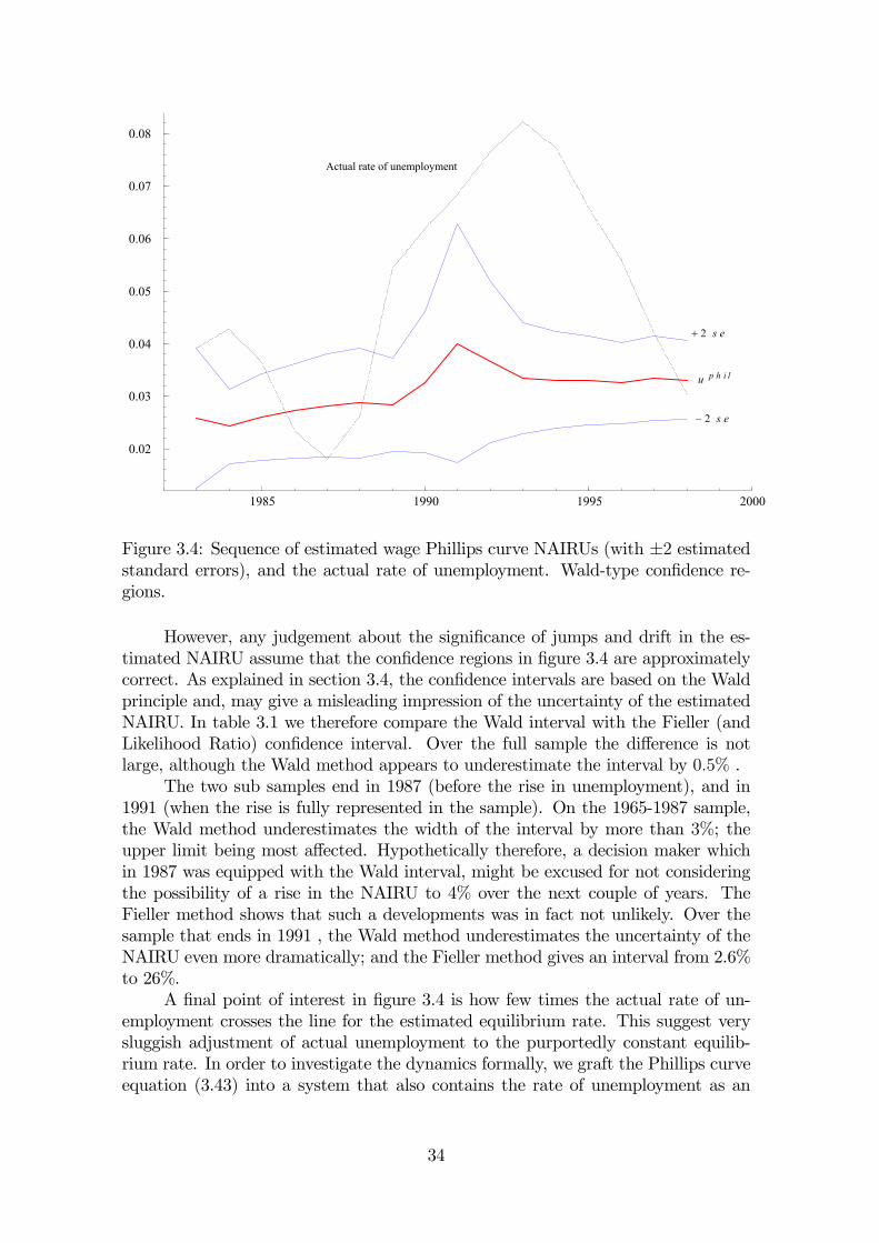
1985 1990 1995 2000
0.02
0.03
0.04
0.05
0.06
0.07
0.08
u p h i l
+ 2 s e
− 2 s e
Actual rate of unemployment
Figure 3.4: Sequence of estimated wage Phillips curve NAIRUs (with ±2 estimatedstandard errors), and the actual rate of unemployment. Wald-type confidence re-gions.
However, any judgement about the significance of jumps and drift in the es-timated NAIRU assume that the confidence regions in figure 3.4 are approximatelycorrect. As explained in section 3.4, the confidence intervals are based on the Waldprinciple and, may give a misleading impression of the uncertainty of the estimatedNAIRU. In table 3.1 we therefore compare the Wald interval with the Fieller (andLikelihood Ratio) confidence interval. Over the full sample the difference is notlarge, although the Wald method appears to underestimate the interval by 0.5% .
The two sub samples end in 1987 (before the rise in unemployment), and in1991 (when the rise is fully represented in the sample). On the 1965-1987 sample,the Wald method underestimates the width of the interval by more than 3%; theupper limit being most affected. Hypothetically therefore, a decision maker whichin 1987 was equipped with the Wald interval, might be excused for not consideringthe possibility of a rise in the NAIRU to 4% over the next couple of years. TheFieller method shows that such a developments was in fact not unlikely. Over thesample that ends in 1991 , the Wald method underestimates the uncertainty of theNAIRU even more dramatically; and the Fieller method gives an interval from 2.6%to 26%.
A final point of interest in figure 3.4 is how few times the actual rate of un-employment crosses the line for the estimated equilibrium rate. This suggest verysluggish adjustment of actual unemployment to the purportedly constant equilib-rium rate. In order to investigate the dynamics formally, we graft the Phillips curveequation (3.43) into a system that also contains the rate of unemployment as an
34
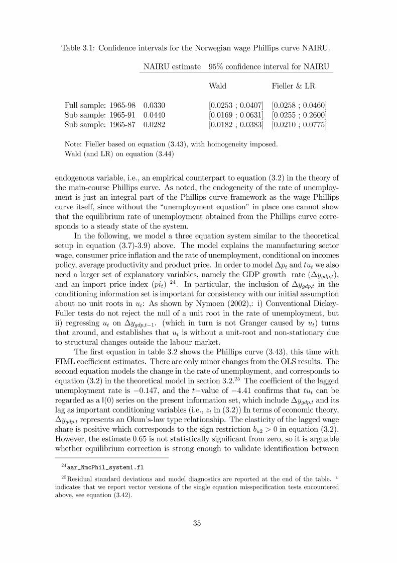
Table 3.1: Confidence intervals for the Norwegian wage Phillips curve NAIRU.
NAIRU estimate 95% confidence interval for NAIRU
Wald Fieller & LR
Full sample: 1965-98 0.0330 [0.0253 ; 0.0407] [0.0258 ; 0.0460]Sub sample: 1965-91 0.0440 [0.0169 ; 0.0631] [0.0255 ; 0.2600]Sub sample: 1965-87 0.0282 [0.0182 ; 0.0383] [0.0210 ; 0.0775]
Note: Fieller based on equation (3.43), with homogeneity imposed.Wald (and LR) on equation (3.44)
endogenous variable, i.e., an empirical counterpart to equation (3.2) in the theory ofthe main-course Phillips curve. As noted, the endogeneity of the rate of unemploy-ment is just an integral part of the Phillips curve framework as the wage Phillipscurve itself, since without the “unemployment equation” in place one cannot showthat the equilibrium rate of unemployment obtained from the Phillips curve corre-sponds to a steady state of the system.
In the following, we model a three equation system similar to the theoreticalsetup in equation (3.7)-3.9) above. The model explains the manufacturing sectorwage, consumer price inflation and the rate of unemployment, conditional on incomespolicy, average productivity and product price. In order to model∆pt and tut we alsoneed a larger set of explanatory variables, namely the GDP growth rate (∆ygdp,t),and an import price index (pit) 24. In particular, the inclusion of ∆ygdp,t in theconditioning information set is important for consistency with our initial assumptionabout no unit roots in ut: As shown by Nymoen (2002),: i) Conventional Dickey-Fuller tests do not reject the null of a unit root in the rate of unemployment, butii) regressing ut on ∆ygdp,t−1. (which in turn is not Granger caused by ut) turnsthat around, and establishes that ut is without a unit-root and non-stationary dueto structural changes outside the labour market.
The first equation in table 3.2 shows the Phillips curve (3.43), this time withFIML coefficient estimates. There are only minor changes from the OLS results. Thesecond equation models the change in the rate of unemployment, and corresponds toequation (3.2) in the theoretical model in section 3.2.25 The coefficient of the laggedunemployment rate is −0.147, and the t−value of −4.41 confirms that tut can beregarded as a I(0) series on the present information set, which include ∆ygdp,t and itslag as important conditioning variables (i.e., zt in (3.2)) In terms of economic theory,∆ygdp,t represents an Okun’s-law type relationship. The elasticity of the lagged wageshare is positive which corresponds to the sign restriction bu2 > 0 in equation (3.2).However, the estimate 0.65 is not statistically significant from zero, so it is arguablewhether equilibrium correction is strong enough to validate identification between
24aar_NmcPhil_system1.fl
25Residual standard deviations and model diagnostics are reported at the end of the table. v
indicates that we report vector versions of the single equation misspecification tests encounteredabove, see equation (3.42).
35
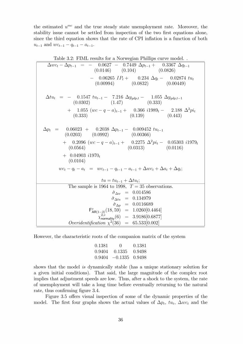
the estimated umc and the true steady state unemployment rate. Moreover, thestability issue cannot be settled from inspection of the two first equations alone,since the third equation shows that the rate of CPI inflation is a function of bothut−1 and wct−1 − qt−1 − at−1.
Table 3.2: FIML results for a Norwegian Phillips curve model. .∆wct −∆pt−1 = − 0.0627
(0.0146)− 0.7449(0.104)
∆pt−1 + 0.3367(0.0826)
∆qt−1
− 0.06265(0.00994)
IPt + 0.234(0.0832)
∆qt − 0.02874(0.00449)
tut
∆tut = − 0.1547(0.0302)
tut−1 − 7.216(1.47)
∆ygdp,t − 1.055(0.333)
∆ygdp,t−1
+ 1.055(0.333)
(wc− q − a)t−1 + 0.366(0.139)
i1989t − 2.188(0.443)
∆2pit
∆pt = 0.06023(0.0203)
+ 0.2038(0.0992)
∆pt−1 − 0.009452(0.00366)
tut−1
+ 0.2096(0.0564)
(wc− q − a)t−1 + 0.2275(0.0313)
∆2pit − 0.05303(0.0116)
i1979t
+ 0.04903(0.0104)
i1970t
wct − qt − at = wct−1 − qt−1 − at−1 +∆wct +∆at +∆qt;
tu = tut−1 +∆tut;The sample is 1964 to 1998, T = 35 observations.
σ∆w = 0.014586σ∆tu = 0.134979σ∆p = 0.0116689
FvAR(1−2)(18, 59) = 1.0260[0.4464]
χ2,vnormality(6) = 3.9186[0.6877]Overidentification χ2(36) = 65.533[0.002]
However, the characteristic roots of the companion matrix of the system
0.1381 0 0.13810.9404 0.1335 0.94980.9404 −0.1335 0.9498
shows that the model is dynamically stable (has a unique stationary solution fora given initial conditions). That said, the large magnitude of the complex rootimplies that adjustment speeds are low. Thus, after a shock to the system, the rateof unemployment will take a long time before eventually returning to the naturalrate, thus confirming figure 3.4.
Figure 3.5 offers visual inspection of some of the dynamic properties of themodel. The first four graphs shows the actual values of ∆pt, tut, ∆wct and the
36
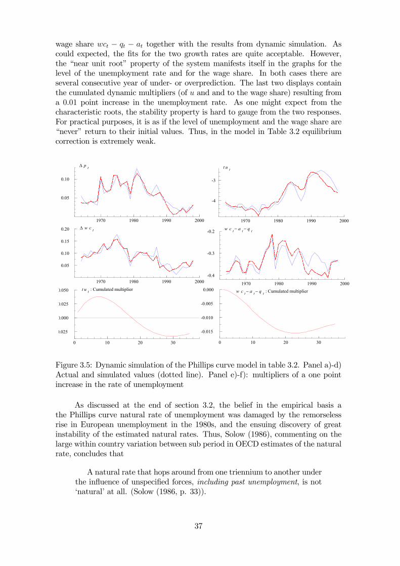
wage share wct − qt − at together with the results from dynamic simulation. Ascould expected, the fits for the two growth rates are quite acceptable. However,the “near unit root” property of the system manifests itself in the graphs for thelevel of the unemployment rate and for the wage share. In both cases there areseveral consecutive year of under- or overprediction. The last two displays containthe cumulated dynamic multipliers (of u and and to the wage share) resulting froma 0.01 point increase in the unemployment rate. As one might expect from thecharacteristic roots, the stability property is hard to gauge from the two responses.For practical purposes, it is as if the level of unemployment and the wage share are“never” return to their initial values. Thus, in the model in Table 3.2 equilibriumcorrection is extremely weak.
1970 1980 1990 2000
0.05
0.10
∆ p t
1970 1980 1990 2000
-4
-3
t u t
1970 1980 1990 2000
0.05
0.10
0.15
0.20 ∆ w c t
1970 1980 1990 2000
-0.4
-0.3
-0.2 w c t − a t − q t
0 10 20 30
0.025
0.000
0.025
0.050 t u t : Cumulated multiplier
0 10 20 30
-0.015
-0.010
-0.005
0.000 w c t − a t − q t : Cumulated multiplier
Figure 3.5: Dynamic simulation of the Phillips curve model in table 3.2. Panel a)-d)Actual and simulated values (dotted line). Panel e)-f): multipliers of a one pointincrease in the rate of unemployment
As discussed at the end of section 3.2, the belief in the empirical basis athe Phillips curve natural rate of unemployment was damaged by the remorselessrise in European unemployment in the 1980s, and the ensuing discovery of greatinstability of the estimated natural rates. Thus, Solow (1986), commenting on thelarge within country variation between sub period in OECD estimates of the naturalrate, concludes that
A natural rate that hops around from one triennium to another underthe influence of unspecified forces, including past unemployment, is not‘natural’ at all. (Solow (1986, p. 33)).
37
In that perspective, the variations in the Norwegian natural rate estimates in figure3.4 are quite modest, and may pass as relatively acceptable as a first order approx-imation of the attainable level of unemployment. However, the econometric systemshowed that equilibrium correction is very weak. After a shock to the system, therate of unemployment is predicted to drift away from the natural rate for a verylong period of time. Hence. the natural rate thesis of asymptotically stability is notvalidated.
There are several responses to this result. First, one might try to patch-upthe estimated unemployment equation, and try to find ways to recover a strongerrelationship between the real wage and the unemployment rate. In the followingwe focus instead on the other end of the problem, namely the Phillips curve itself.In section 5.8.2 we show that when the Phillips curve framework is replaced with awage model that allows equilibrium correction to any given rate of unemploymentrather than to only the “natural rate”, all the inconsistencies are resolved. However,that kind of wage equation is first anchored in the economic theory of section 4 and5.
3.7 SummaryThe Phillips curve ranges as the dominant approach to wage and price modellingin macroeconomics. In the US, in particular, it retains its role as the operationalframework for both inflation forecasting and for estimating of the NAIRU. In thissection we have shown that the Phillips curve is consistent with cointegration be-tween prices, wages and productivity and a stationary rate of unemployment, andhence there is a common ground between the Phillips curve and the Norwegianmodel of inflation of the previous section. However, unlike the Norwegian model,the Phillips curve framework specifies a single equilibrating mechanism which sup-port cointegration–in the simplest case with fixed and exogenous labour supply,the equilibrium correction is due to a downward sloping labour demand schedule.The specificity of the equilibrating mechanism of the Phillips curve is not alwaysrecognized. In the context of macroeconomic models with a large number of equa-tions, it has the somewhat paradoxical implication that the stationary value of therate of unemployment can be estimated from a single equation.
We have also argued that the Phillips curve framework is consistent with astable autoregressive process for the rate of unemployment, subject only to a fewregime shift that can be identified with structural breaks in the operation of labourmarkets. The development of European unemployment rates since the early 1980s isdifficult to fit into this framework, and model builders started to look for alternativemodels. Interestingly, already in 1984 one review of the UK macroeconomic modelsconcluded that “developments in wage equations have led to the virtual demise ofthe Phillips curve as the standard wage relationship in macromodels ”26. These newdevelopments are the theme of the two next sections.
26See Wallis et al. (1984, p. 134).
38
4 Wage bargaining and price setting
In the course of the 1980s interesting developments took place in macroeconomics.First, the macroeconomic implications of imperfect competition with price-settingfirms were developed in several papers and books, see e.g., Bruno (1979), and Blan-chard and Kiyotaki (1987), Bruno and Sachs (1984) and Blanchard and Fisher (1989,Chapter 8). Second, the economic theory of labour unions, pioneered by Dun-lop (1944), was extended and formalized in a game theoretic framework, see e.g.,Nickell and Andrews (1983), Hoel and Nymoen (1988). Models of European unem-ployment, that incorporated elements from both these developments, appeared inLayard and Nickell (1986), Layard et al. (1991), Carlin and Soskice (1990) and Lind-beck (1993). The new standard model of European unemployment is incontestablylinked to Layard and Nickell and their coauthors. However, we follow establishedpractice and refer to the framework as the Incomplete Competiton Model (ICM),or, interchangeably, as the wage curve framework (as opposed to the Phillips curvemodel of the previous section). Incomple competition, is particualrly apt since themodel’s defining characteristic is the explicit assumption of imperfect competitionin both product and labour markets, see e.g., Carlin and Soskice (1990).27 TheICM was quickly incorporated into the supply side of macroconometric models, seeWallis (1993, 1995), and purged European econometric models of the Phillips curve,at least until the arrival of the New Keynesian Phillips curve late in the 1990s (seesection 6 in this book)
Since the theory is cast in terms of levels variables, the ICM stands closer tothe main course model than the Phillips curve tradition. On the other hand, boththe wage curve and the Phillips curve presume that it is the rate of unemploymentthat reconciles the conflict between wage earners and firms. Both models take theview that the equilibrium or steady state rate of unemployment is determined bya limited number of factors that reflect structural aspect such as production tech-nology, union preferences and institutional factors (characteristics of the bargainingsystem, the unemployment insurance system). Thus, in both families of theories de-mand management and monetary policy have only a short term effect on the rate ofunemployment. In the (hypothetical) situation when all shocks are switched off, therate of unemployment would return to a unique structural equilibrium rate, i.e. thenatural rate or the NAIRU. Thus, the ICM is unmistakably a model of the naturalrate both in its motivation and in its implications: “In the long run, unemploymentis determined entirely by long-run supply factors and equals the NAIRU.”(Layardet al. (1994, p 23)).
4.1 Wage bargaining and monopolistic competitionThere is a number of specialized models of “non competitive” wage setting, see e.g.,Layard et al. (1991, Chapter 7). Our aim in this section is to represent the commonfeatures of these approaches in a model of theoretical model of wage bargaining andmonopolistic competition, building on Rødseth (2000, Ch. 5.9) and Nymoen andRødseth (2003). We start with the assumption of a large number of firms, each
27Nevertheless, the ICM acrynom may be confusing, in particular if it is taken to imply that thealternative model (the Phillip curve) contain perfect competition.
39
facing downward-sloping demand functions. The firms are price setters and equatemarginal revenue to marginal costs. With labour being the only variable factorof production (and constant returns to scale) we obtain the following price settingrelationship
Qi =ElQY
ElQY − 1Wi
Ai
where Ai = Yi/Ni is average labour productivity Yi is output and Ni is labourinput. ElQY > 1 denotes the absolute value of the elasticity of demand facing eachfirm i with respect to the firm’s own price. In general ElQY is a function of relativeprices, which provides a rationale for inclusion of e.g., the real exchange rate inaggregate price equations. However, it is a common simplification to assume thatthe elasticity is independent of other firms prices and is identical for all firms. Withconstant returns technology aggregation is no problem, but for simplicity we assumethat average labour productivity is the same for all firms and that the aggregateprice equation is given by
(4.1) Q =ElQY
ElQY − 1W
A
The expression for real profits (π) is therefore
π = Y − W
QN = (1− W
Q
1
A)Y.
We assume that the wageW is settled in accordance with the principle of maximizingof the Nash-product:
(4.2) (ν − ν0)fπ1−f
where ν denotes union utility and ν0 denotes the fall-back utility or reference utility.The corresponding break-point utility for the firms has already been set to zero in(4.2), but for unions the utility during a conflict (e.g., strike, or work-to-rule) isnon-zero because of compensation from strike funds. Finally f is represents therelative bargaining power of unions.
Union utility depends on the consumer real wage of an unemployed worker andthe aggregate rate of unemployment, thus ν(W
P, U, Zν) where P denotes the consumer
price index.28 The partial derivative with respect to wages is positive, and negativewith respect to unemployment (ν 0W > 0 and ν 0U ≤ 0). Zν represents other factorsin union preferences. The fall-back or reference utility of the union depends on theoverall real wage level and the rate of unemployment, hence ν0 = ν0(
WP, U) where
W is the average level of nominal wages which is one of factors determining the sizeof strike funds. If the aggregate rate of unemployment is high, strike funds may runlow in which case the partial derivative of ν0 with respect to U is negative (ν 00U < 0).However, there are other factors working in the other direction, for example thatthe probability of entering a labour market programme, which gives laid-off workershigher utility than open unemployment, is positively related to U . Thus, the sign
28We abstract from a proportional income tax rate.
40
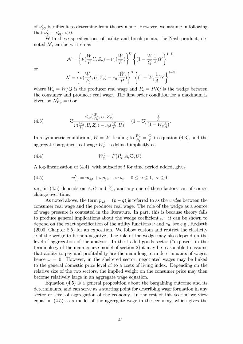
of ν 00U is difficult to determine from theory alone. However, we assume in followingthat ν 0U − ν 00U < 0.
With these specifications of utility and break-points, the Nash-product, de-noted N , can be written as
N =
½ν(W
PU,Zν)− ν0(
W
P)
¾f ½(1− W
Q
1
A)Y
¾1−for
N =
½ν(Wq
Pq, U, Zν)− ν0(
W
P)
¾f ½(1−Wq
1
A)Y
¾1−fwhere Wq = W/Q is the producer real wage and Pq = P/Q is the wedge betweenthe consumer and producer real wage. The first order condition for a maximum isgiven by NWq = 0 or
(4.3) fν0W (
Wq
Pq, U, Zν)
ν(Wq
Pq, U, Zν)− ν0(
WP, U)
= (1−f)1A
(1−Wq1A).
In a symmetric equilibrium, W = W , leading to Wq
Pq= W
Pin equation (4.3), and the
aggregate bargained real wage W bq is defined implicitly as
(4.4) W bq = F (Pq, A,f, U).
A log-linearization of (4.4), with subscript t for time period added, gives
(4.5) wbq,t = mb,t + ωpq,t − ut, 0 ≤ ω ≤ 1, ≥ 0.
mb,t in (4.5) depends on A,f and Zν , and any one of these factors can of coursechange over time.
As noted above, the term pq,t = (p− q)tis referred to as the wedge between theconsumer real wage and the producer real wage. The role of the wedge as a sourceof wage pressure is contested in the literature. In part, this is because theory failsto produce general implications about the wedge coefficient ω–it can be shown todepend on the exact specification of the utility functions ν and ν0, see e.g., Rødseth(2000, Chapter 8.5) for an exposition. We follow custom and restrict the elasticityω of the wedge to be non-negative. The role of the wedge may also depend on thelevel of aggregation of the analysis. In the traded goods sector (“exposed” in theterminology of the main course model of section 2) it may be reasonable to assumethat ability to pay and profitability are the main long term determinants of wages,hence ω = 0. However, in the sheltered sector, negotiated wages may be linkedto the general domestic price level of to a costs of living index. Depending on therelative size of the two sectors, the implied weight on the consumer price may thenbecome relatively large in an aggregate wage equation.
Equation (4.5) is a general proposition about the bargaining outcome and itsdeterminants, and can serve as a starting point for describing wage formation in anysector or level of aggregation of the economy. In the rest of this section we viewequation (4.5) as a model of the aggregate wage in the economy, which gives the
41
log of real wage
i
iii
ii
log of rate ofunemployment
'low'
''high'
Figure 4.1: Role of degree of wage responsiveness to unemployment
most direct route to the predicted equilibrium outcome for real wages and for therate of unemployment. However, in section 4.3 we consider another frequently madeinterpretation, namely that equation (4.5) applies to the manufacturing sector.
The impact of the rate of unemployment on the bargained wage is given by theelasticity , which is a key parameter of interest in the wage curve literature. mayvary between countries according to different wages setting system. For example,a high degree coordination, especially on the employer side and centralization ofbargaining is expected to induce more responsiveness to unemployment (a higher )than uncoordinated systems that give little incentives to solidaristic bargaining. Atleast this is the view expressed by authors who build on multi-country regressions,see e.g., Alogoskoufis and Manning (1988) and Layard et al. (1991, Chapter 9).However, this view is not always shared by economists with detailed knowledge ofe.g., the Swedish system of centralized bargaining, see Lindbeck (1993, Chapter 8).
Figure 4.1 also motivates why the magnitude of plays such an importantrole in the wage curve literature. The horizontal line in the figure is consistent withthe equation for price setting in (4.1),under the assumption that productivity isindependent of unemployment (‘normal cost pricing’). The two downward slopinglines labeled ‘low’ and ‘high’ (wage responsiveness), represent different states ofwage setting, namely ‘low’ and ‘high’ . Point i) in the figure represents a situationin which firm’s wage setting and the bargaining outcome are consistent in bothcountries–we can think of this as a low unemployment equilibrium. Next, assumethat the two economies are hit by a supply-side shock, that shifts the firm-side realwage down to the dotted line. The Layard-Nickell model implies that the economy
42
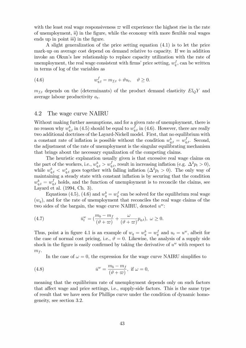
with the least real wage responsiveness will experience the highest rise in the rateof unemployment, ii) in the figure, while the economy with more flexible real wagesends up in point iii) in the figure.
A slight generalization of the price setting equation (4.1) is to let the pricemark-up on average cost depend on demand relative to capacity. If we in additioninvoke an Okun’s law relationship to replace capacity utilization with the rate ofunemployment, the real wage consistent with firms’ price setting, wf
q , can be writtenin terms of log of the variables as
(4.6) wfq,t = mf,t + ϑut, ϑ ≥ 0.
mf,t depends on the (determinants) of the product demand elasticity ElQY andaverage labour productivity at.
4.2 The wage curve NAIRUWithout making further assumptions, and for a given rate of unemployment, there isno reason why wb
q,t in (4.5) should be equal to wfq,t in (4.6). However, there are really
two additional doctrines of the Layard-Nickell model. First, that no equilibriumwitha constant rate of inflation is possible without the condition wb
q,t = wfq,t. Second,
the adjustment of the rate of unemployment is the singular equilibrating mechanismthat brings about the necessary equalization of the competing claims.
The heuristic explanation usually given is that excessive real wage claims onthe part of the workers, i.e., wb
q,t > wfq,t, result in increasing inflation (e.g. ∆
2pt > 0),while wb
q,t < w∗q,t goes together with falling inflation (∆2pt > 0). The only way of
maintaining a steady state with constant inflation is by securing that the conditionwbq,t = wf
q,t holds, and the function of unemployment is to reconcile the claims, seeLayard et al. (1994, Ch. 3).
Equations (4.5), (4.6) and wbq = wf
q can be solved for the equilibrium real wage(wq), and for the rate of unemployment that reconciles the real wage claims of thetwo sides of the bargain, the wage curve NAIRU, denoted uw:
(4.7) uwt = (mb −mf
(ϑ+ )+
ω
(ϑ+ )pq,t), ω ≥ 0.
Thus, point a in figure 4.1 is an example of wq = wbq = wf
q and ut = uw, albeit forthe case of normal cost pricing, i.e., ϑ = 0. Likewise, the analysis of a supply sideshock in the figure is easily confirmed by taking the derivative of uw with respect tomf .
In the case of ω = 0, the expression for the wage curve NAIRU simplifies to
(4.8) uw =mb −mf
(ϑ+ ), if ω = 0,
meaning that the equilibrium rate of unemployment depends only on such factorsthat affect wage and price settings, i.e., supply-side factors. This is the same typeof result that we have seen for Phillips curve under the condition of dynamic homo-geneity, see section 3.2.
43
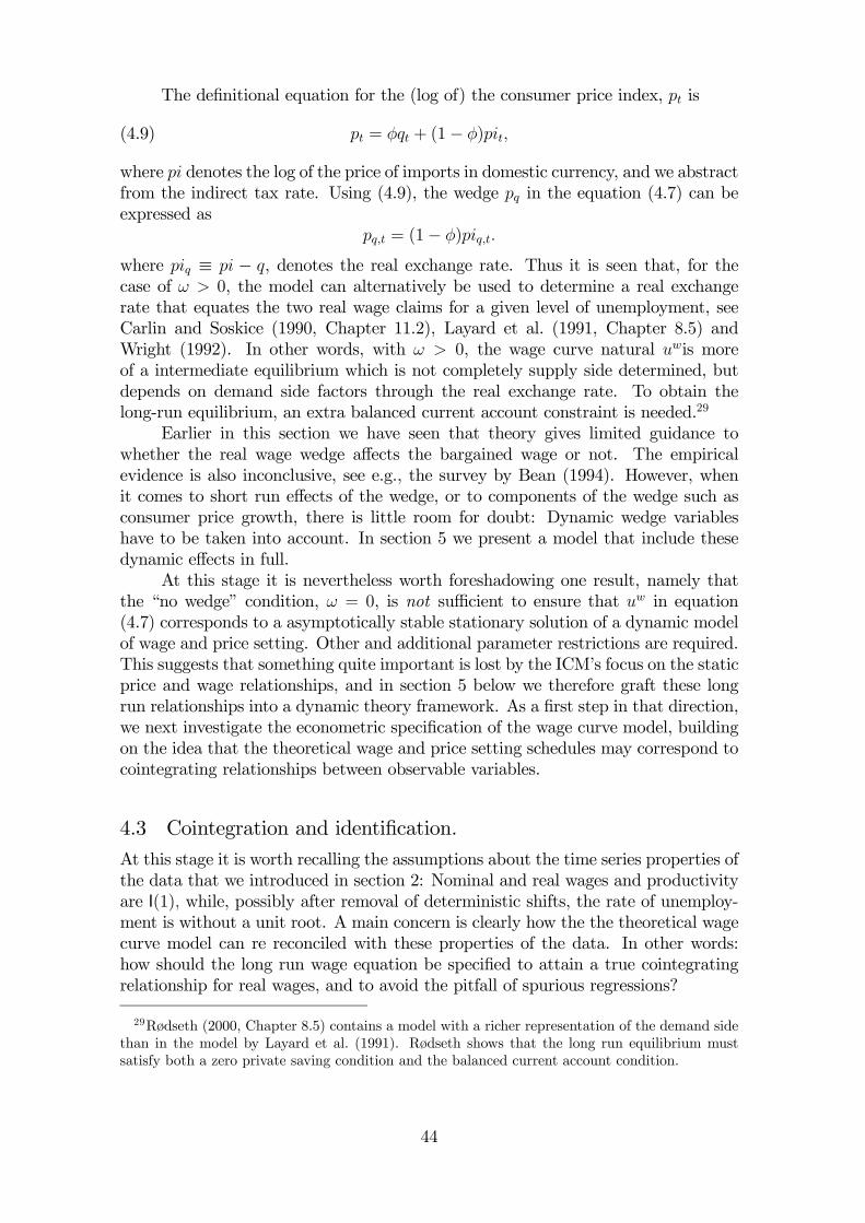
The definitional equation for the (log of) the consumer price index, pt is
(4.9) pt = φqt + (1− φ)pit,
where pi denotes the log of the price of imports in domestic currency, and we abstractfrom the indirect tax rate. Using (4.9), the wedge pq in the equation (4.7) can beexpressed as
pq,t = (1− φ)piq,t.
where piq ≡ pi − q, denotes the real exchange rate. Thus it is seen that, for thecase of ω > 0, the model can alternatively be used to determine a real exchangerate that equates the two real wage claims for a given level of unemployment, seeCarlin and Soskice (1990, Chapter 11.2), Layard et al. (1991, Chapter 8.5) andWright (1992). In other words, with ω > 0, the wage curve natural uwis moreof a intermediate equilibrium which is not completely supply side determined, butdepends on demand side factors through the real exchange rate. To obtain thelong-run equilibrium, an extra balanced current account constraint is needed.29
Earlier in this section we have seen that theory gives limited guidance towhether the real wage wedge affects the bargained wage or not. The empiricalevidence is also inconclusive, see e.g., the survey by Bean (1994). However, whenit comes to short run effects of the wedge, or to components of the wedge such asconsumer price growth, there is little room for doubt: Dynamic wedge variableshave to be taken into account. In section 5 we present a model that include thesedynamic effects in full.
At this stage it is nevertheless worth foreshadowing one result, namely thatthe “no wedge” condition, ω = 0, is not sufficient to ensure that uw in equation(4.7) corresponds to a asymptotically stable stationary solution of a dynamic modelof wage and price setting. Other and additional parameter restrictions are required.This suggests that something quite important is lost by the ICM’s focus on the staticprice and wage relationships, and in section 5 below we therefore graft these longrun relationships into a dynamic theory framework. As a first step in that direction,we next investigate the econometric specification of the wage curve model, buildingon the idea that the theoretical wage and price setting schedules may correspond tocointegrating relationships between observable variables.
4.3 Cointegration and identification.At this stage it is worth recalling the assumptions about the time series properties ofthe data that we introduced in section 2: Nominal and real wages and productivityare I(1), while, possibly after removal of deterministic shifts, the rate of unemploy-ment is without a unit root. A main concern is clearly how the the theoretical wagecurve model can re reconciled with these properties of the data. In other words:how should the long run wage equation be specified to attain a true cointegratingrelationship for real wages, and to avoid the pitfall of spurious regressions?
29Rødseth (2000, Chapter 8.5) contains a model with a richer representation of the demand sidethan in the model by Layard et al. (1991). Rødseth shows that the long run equilibrium mustsatisfy both a zero private saving condition and the balanced current account condition.
44
As we have seen, according to the bargaining theory, the term mb,t in (4.5)depends on average productivity, At.30 Having assumed ut ∼ I(0), and keeping inmind the possibility that ω = 0, it is seen that it follows directly from cointegrationthat productivity has to be an important variable in the relationship. In other words,a positive elasticity ElAWq is required to balance the I(1)- trend in the product realwage on the left hand side of the expression.
Thus, the general long run wage equation implied by the wage bargainingapproach becomes
(4.10) wbq,t = mb + ιat + ωpq,t − ut, 0 < ι ≤ 1, 0 ≤ ω ≤ 1, ≥ 0,
where wbq,t ≡ wb
t − qt denotes the “bargained real wage” as before. It is understoodthat the intercept mb is redefined without the productivity term, which is nowsingled out as an I(1) variable in the left hand side of the expression, and with theother determinants assumed to be constant. Finally, defining
ecmb,t= wq,t − wbq,t ∼ I(0)
allows us to write the hypothesized cointegrating wage equation as
(4.11) wq,t = mb + ιat + ωpq,t − ut + ecmb,t.
Some writers prefer to include the reservation wage (the wage equivalent of beingunemployed) in (4.10). For example, from Blanchard and Katz (1999) (but usingour own notation to express their ideas):
(4.12) wbq,t = mb + ι0at + (1− ι0)wr
t + ωpq,t − ut, 0 < ι0 ≤ 1
where wr denotes the reservation wage. However, since real wages are integrated, anymeaningful operational measure of wr
t must logically cointegrate with wq,t directly.In fact, Blanchard and Katz hypothesize that wr is a linear function of the realwage and the level of productivity.31 Using that (second) cointegrating relationship)to substitute out wr
t from (4.12) implies a relationship which is observationallyequivalent to (??).
The cointegration relationship stemming from price setting is anchored in equa-tion (4.6) of the previous section. In the same way as for wage setting, it becomesimportant in applied work to represent the productivity term explicitly in the rela-tionship. We therefore re-write the long term price setting schedule as
(4.13) wfq,t = mf + at + ϑut
30Recall that we expressed the Nash-product as
fν0W (
Wq
Pq, U, Zν)
ν(Wq
Pq, U, Zν)− ν0(
Wq
Pq, U)
= (1− f)1A
(1−Wq1A),
in (4.3).31cf., their equation (4), which uses the lagged real wage on the reight hand side, but lagged real
wages naturally cointegrate with current real wage.
45
where the composite term mf in (4.6) has been replaced by mf + at. Introducingecmf,t = wq,t − wf
q,t ∼ I(0), the second implied cointegration relationship becomes(4.14) wq,t = mf + at + ϑut + ecmf,t.
While the two cointegrating relationships are not identified in general, identify-ing restrictions can be shown to apply in specific situations that occur frequently inapplied work. Our own experience from modelling both disaggregate and aggregatedata, the following three “identification schemes” have proven themselves useful:
One cointegrating vector. In many applications, especially on sectorialdata, formal tests of cointegration support only one cointegration relationship, thuseither one of ecmb,t and ecmf,t is I(1), instead of both being I(0). In this caseit is usually possible to identify the single cointegrating equation economically byrestricting the coefficients, and by testing the weak exogeneity of one or more of thevariables in the system.
No wedge. Second, and still thinking in terms of a sectorial wage-pricesystem: Assume that the price-mark up is not constant as assumed above, but afunction of the relative price (via the price elasticity ). In this case, the priceequation (4.14) is augmented by the real exchange rate pt − pit. If we furthermoreassume that ω = 0, (no wedge in wage formation) and ϑ = 0 (normal cost pricing),identification of both long run schedules is logically possible.
Aggregate price-wage model. The third cointegrating identification schemeis suited for the case of aggregated wages and prices. The long-run model is
wt = mb + (1− ω) qt + ιat + ωpt − ut + ecmb,t(4.15)
qt = −mf + wt − at − ϑut − ecmf,t(4.16)
pt = φqt + (1− φ)pit
solving out for producer prices qt then gives a model in wages wt and consumerprices pt only,
wt = mb +1− ω (1− φ)
φpt(4.17)
+ιat − ut − (1− ω) (1− φ)
φpit +
(1− ω)
φecmb,t
pt = −φmf + φ (wt − at)(4.18)
−φϑut + (1− φ)pit − φecmf,t,
that implicitly implies non-linear cross-equation restrictions in terms of φ.Simply by viewing (4.15) and (4.16) as a pair of simultaneous equations, it
is clear that the system is unidentified in general. However, if the high level ofaggregation means that ω can be set to unity (while retaining cointegration), andat there is normal cost pricing in the aggregated price relationship identificationis again possible. Thus ω = 1 and ϑ = 0 represents one set of necessary (order)restrictions for identification in this case:
wt = mb + pt + ιat − ut(4.19)
pt = −φmf + φ (wt − at) + (1− φ)pit − φecmf,t.(4.20)
46
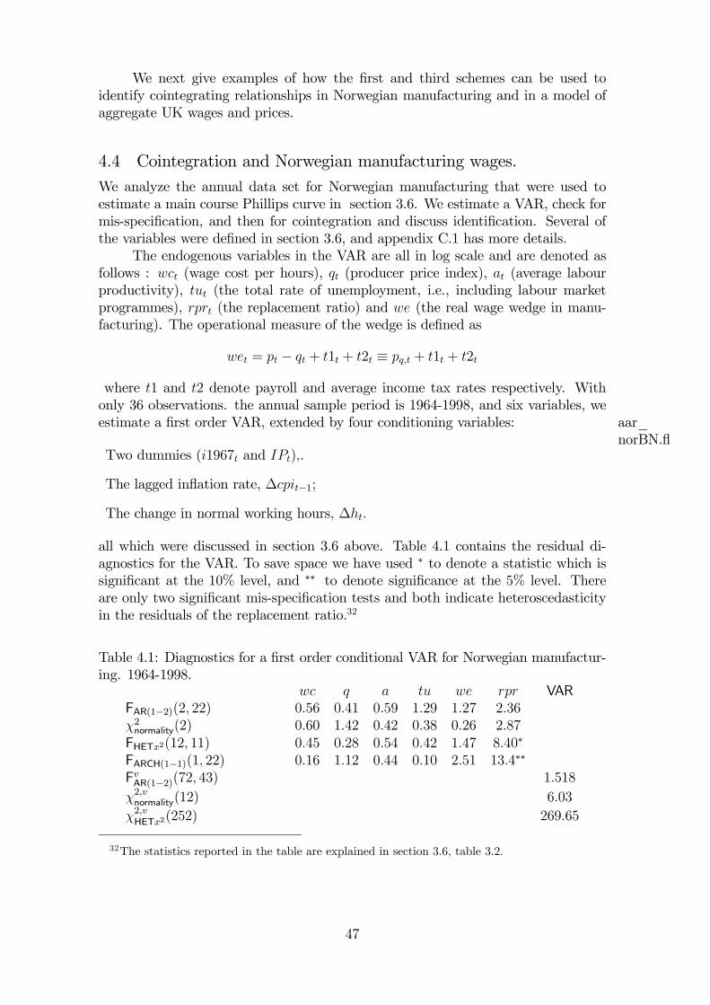
We next give examples of how the first and third schemes can be used toidentify cointegrating relationships in Norwegian manufacturing and in a model ofaggregate UK wages and prices.
4.4 Cointegration and Norwegian manufacturing wages.We analyze the annual data set for Norwegian manufacturing that were used toestimate a main course Phillips curve in section 3.6. We estimate a VAR, check formis-specification, and then for cointegration and discuss identification. Several ofthe variables were defined in section 3.6, and appendix C.1 has more details.
The endogenous variables in the VAR are all in log scale and are denoted asfollows : wct (wage cost per hours), qt (producer price index), at (average labourproductivity), tut (the total rate of unemployment, i.e., including labour marketprogrammes), rprt (the replacement ratio) and we (the real wage wedge in manu-facturing). The operational measure of the wedge is defined as
wet = pt − qt + t1t + t2t ≡ pq,t + t1t + t2t
where t1 and t2 denote payroll and average income tax rates respectively. Withonly 36 observations. the annual sample period is 1964-1998, and six variables, weestimate a first order VAR, extended by four conditioning variables: aar_
norBN.flTwo dummies (i1967t and IPt),.
The lagged inflation rate, ∆cpit−1;
The change in normal working hours, ∆ht.
all which were discussed in section 3.6 above. Table 4.1 contains the residual di-agnostics for the VAR. To save space we have used ∗ to denote a statistic which issignificant at the 10% level, and ∗∗ to denote significance at the 5% level. Thereare only two significant mis-specification tests and both indicate heteroscedasticityin the residuals of the replacement ratio.32
Table 4.1: Diagnostics for a first order conditional VAR for Norwegian manufactur-ing. 1964-1998.
wc q a tu we rpr VARFAR(1−2)(2, 22) 0.56 0.41 0.59 1.29 1.27 2.36χ2normality(2) 0.60 1.42 0.42 0.38 0.26 2.87FHETx2(12, 11) 0.45 0.28 0.54 0.42 1.47 8.40∗
FARCH(1−1)(1, 22) 0.16 1.12 0.44 0.10 2.51 13.4∗∗
FvAR(1−2)(72, 43) 1.518
χ2,vnormality(12) 6.03
χ2,vHETx2(252) 269.65
32The statistics reported in the table are explained in section 3.6, table 3.2.
47
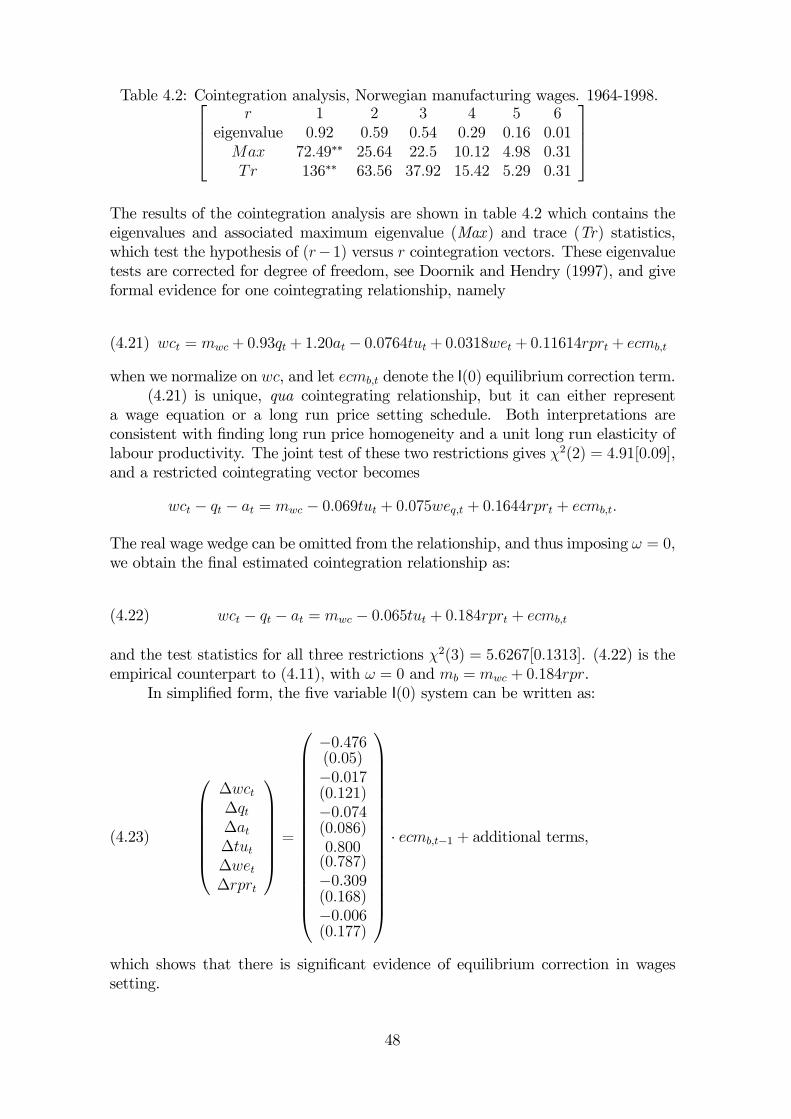
Table 4.2: Cointegration analysis, Norwegian manufacturing wages. 1964-1998.r 1 2 3 4 5 6
eigenvalue 0.92 0.59 0.54 0.29 0.16 0.01Max 72.49∗∗ 25.64 22.5 10.12 4.98 0.31Tr 136∗∗ 63.56 37.92 15.42 5.29 0.31
The results of the cointegration analysis are shown in table 4.2 which contains theeigenvalues and associated maximum eigenvalue (Max) and trace (Tr) statistics,which test the hypothesis of (r−1) versus r cointegration vectors. These eigenvaluetests are corrected for degree of freedom, see Doornik and Hendry (1997), and giveformal evidence for one cointegrating relationship, namely
(4.21) wct = mwc + 0.93qt + 1.20at − 0.0764tut + 0.0318wet + 0.11614rprt + ecmb,t
when we normalize on wc, and let ecmb,t denote the I(0) equilibrium correction term.(4.21) is unique, qua cointegrating relationship, but it can either represent
a wage equation or a long run price setting schedule. Both interpretations areconsistent with finding long run price homogeneity and a unit long run elasticity oflabour productivity. The joint test of these two restrictions gives χ2(2) = 4.91[0.09],and a restricted cointegrating vector becomes
wct − qt − at = mwc − 0.069tut + 0.075weq,t + 0.1644rprt + ecmb,t.
The real wage wedge can be omitted from the relationship, and thus imposing ω = 0,we obtain the final estimated cointegration relationship as:
(4.22) wct − qt − at = mwc − 0.065tut + 0.184rprt + ecmb,t
and the test statistics for all three restrictions χ2(3) = 5.6267[0.1313]. (4.22) is theempirical counterpart to (4.11), with ω = 0 and mb = mwc + 0.184rpr.
In simplified form, the five variable I(0) system can be written as:
(4.23)
∆wct∆qt∆at∆tut∆wet∆rprt
=
−0.476(0.05)−0.017(0.121)−0.074(0.086)0.800(0.787)−0.309(0.168)−0.006(0.177)
· ecmb,t−1 + additional terms,
which shows that there is significant evidence of equilibrium correction in wagessetting.
48
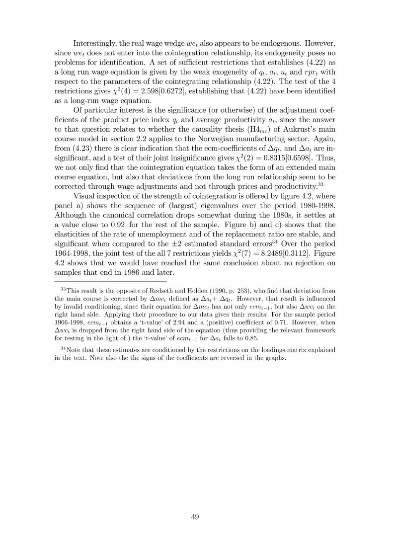
Interestingly, the real wage wedgewet also appears to be endogenous. However,since wet does not enter into the cointegration relationship, its endogeneity poses noproblems for identification. A set of sufficient restrictions that establishes (4.22) asa long run wage equation is given by the weak exogeneity of qt, at, ut and rprt withrespect to the parameters of the cointegrating relationship (4.22). The test of the 4restrictions gives χ2(4) = 2.598[0.6272], establishing that (4.22) have been identifiedas a long-run wage equation.
Of particular interest is the significance (or otherwise) of the adjustment coef-ficients of the product price index qt and average productivity at, since the answerto that question relates to whether the causality thesis (H4mc) of Aukrust’s maincourse model in section 2.2 applies to the Norwegian manufacturing sector. Again,from (4.23) there is clear indication that the ecm-coefficients of ∆qt, and ∆at are in-significant, and a test of their joint insignificance gives χ2(2) = 0.8315[0.6598]. Thus,we not only find that the cointegration equation takes the form of an extended maincourse equation, but also that deviations from the long run relationship seem to becorrected through wage adjustments and not through prices and productivity.33
Visual inspection of the strength of cointegration is offered by figure 4.2, wherepanel a) shows the sequence of (largest) eigenvalues over the period 1980-1998.Although the canonical correlation drops somewhat during the 1980s, it settles ata value close to 0.92 for the rest of the sample. Figure b) and c) shows that theelasticities of the rate of unemployment and of the replacement ratio are stable, andsignificant when compared to the ±2 estimated standard errors34 Over the period1964-1998, the joint test of the all 7 restrictions yields χ2(7) = 8.2489[0.3112]. Figure4.2 shows that we would have reached the same conclusion about no rejection onsamples that end in 1986 and later.
33This result is the opposite of Rødseth and Holden (1990, p. 253), who find that deviation fromthe main course is corrected by ∆mct defined as ∆at+ ∆qt. However, that result is influencedby invalid conditioning, since their equation for ∆mct has not only ecmt−1, but also ∆wct on theright hand side. Applying their procedure to our data gives their results: For the sample period1966-1998, ecmt−1 obtains a ‘t-value’ of 2.94 and a (positive) coefficient of 0.71. However, when∆wct is dropped from the right hand side of the equation (thus providing the relevant frameworkfor testing in the light of ) the ‘t-value’ of ecmt−1 for ∆at falls to 0.85.34Note that these estimates are conditioned by the restrictions on the loadings matrix explained
in the text. Note also the the signs of the coefficients are reversed in the graphs.
49
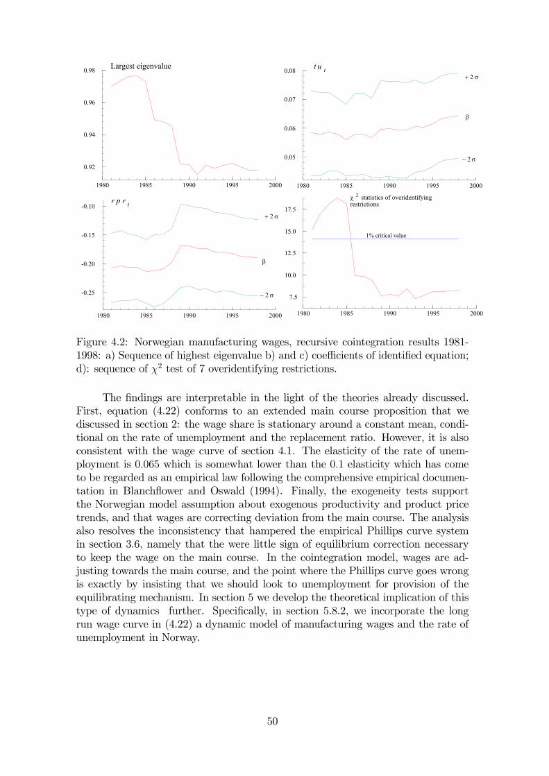
1980 1985 1990 1995 2000
0.92
0.94
0.96
0.98 Largest eigenvalue
1980 1985 1990 1995 2000
0.05
0.06
0.07
0.08
β
+ 2 σ
− 2 σ
t u t
1980 1985 1990 1995 2000
-0.25
-0.20
-0.15
-0.10
− 2 σ
+ 2 σ
β
r p r t
1980 1985 1990 1995 2000
7.5
10.0
12.5
15.0
17.5
χ 2 statistics of overidentifyingrestrictions
1% critical value
Figure 4.2: Norwegian manufacturing wages, recursive cointegration results 1981-1998: a) Sequence of highest eigenvalue b) and c) coefficients of identified equation;d): sequence of χ2 test of 7 overidentifying restrictions.
The findings are interpretable in the light of the theories already discussed.First, equation (4.22) conforms to an extended main course proposition that wediscussed in section 2: the wage share is stationary around a constant mean, condi-tional on the rate of unemployment and the replacement ratio. However, it is alsoconsistent with the wage curve of section 4.1. The elasticity of the rate of unem-ployment is 0.065 which is somewhat lower than the 0.1 elasticity which has cometo be regarded as an empirical law following the comprehensive empirical documen-tation in Blanchflower and Oswald (1994). Finally, the exogeneity tests supportthe Norwegian model assumption about exogenous productivity and product pricetrends, and that wages are correcting deviation from the main course. The analysisalso resolves the inconsistency that hampered the empirical Phillips curve systemin section 3.6, namely that the were little sign of equilibrium correction necessaryto keep the wage on the main course. In the cointegration model, wages are ad-justing towards the main course, and the point where the Phillips curve goes wrongis exactly by insisting that we should look to unemployment for provision of theequilibrating mechanism. In section 5 we develop the theoretical implication of thistype of dynamics further. Specifically, in section 5.8.2, we incorporate the longrun wage curve in (4.22) a dynamic model of manufacturing wages and the rate ofunemployment in Norway.
50
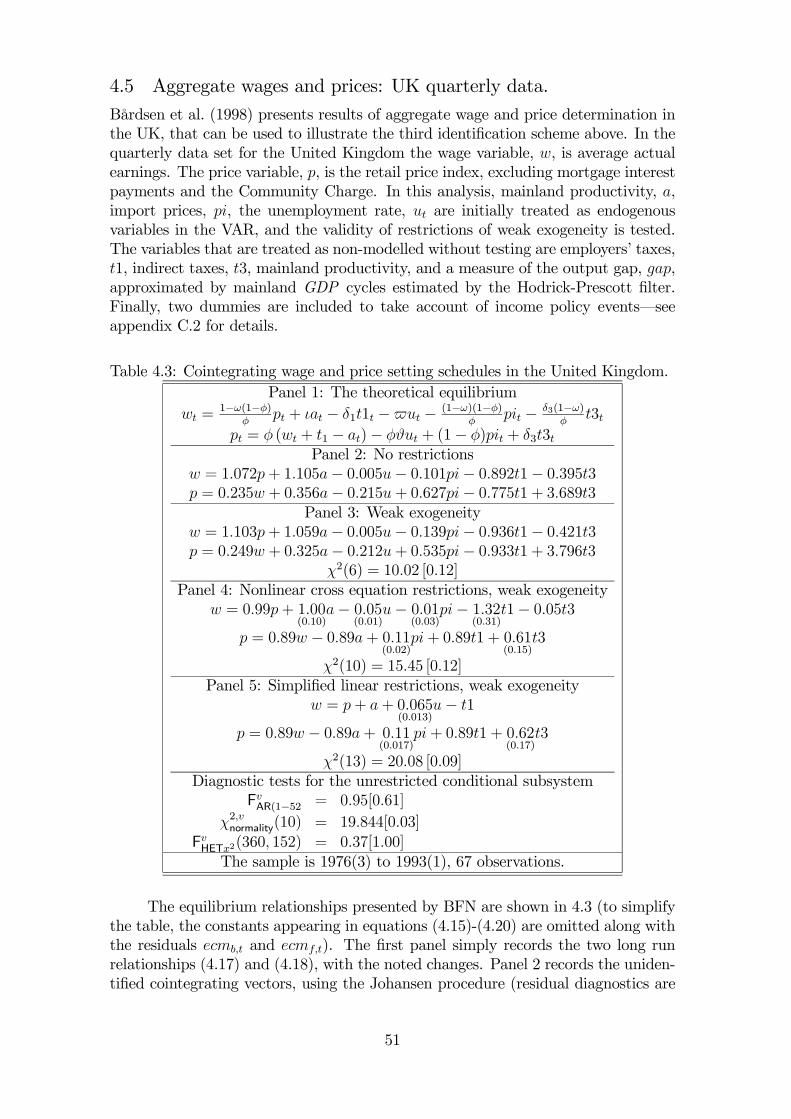
4.5 Aggregate wages and prices: UK quarterly data.Bårdsen et al. (1998) presents results of aggregate wage and price determination inthe UK, that can be used to illustrate the third identification scheme above. In thequarterly data set for the United Kingdom the wage variable, w, is average actualearnings. The price variable, p, is the retail price index, excluding mortgage interestpayments and the Community Charge. In this analysis, mainland productivity, a,import prices, pi, the unemployment rate, ut are initially treated as endogenousvariables in the VAR, and the validity of restrictions of weak exogeneity is tested.The variables that are treated as non-modelled without testing are employers’ taxes,t1, indirect taxes, t3, mainland productivity, and a measure of the output gap, gap,approximated by mainland GDP cycles estimated by the Hodrick-Prescott filter.Finally, two dummies are included to take account of income policy events–seeappendix C.2 for details.
Table 4.3: Cointegrating wage and price setting schedules in the United Kingdom.Panel 1: The theoretical equilibrium
wt =1−ω(1−φ)
φpt + ιat − δ1t1t − ut − (1−ω)(1−φ)
φpit − δ3(1−ω)
φt3t
pt = φ (wt + t1 − at)− φϑut + (1− φ)pit + δ3t3tPanel 2: No restrictions
w = 1.072p+ 1.105a− 0.005u− 0.101pi− 0.892t1− 0.395t3p = 0.235w + 0.356a− 0.215u+ 0.627pi− 0.775t1 + 3.689t3
Panel 3: Weak exogeneityw = 1.103p+ 1.059a− 0.005u− 0.139pi− 0.936t1− 0.421t3p = 0.249w + 0.325a− 0.212u+ 0.535pi− 0.933t1 + 3.796t3
χ2(6) = 10.02 [0.12]Panel 4: Nonlinear cross equation restrictions, weak exogeneity
w = 0.99p+ 1.00(0.10)
a− 0.05(0.01)
u− 0.01(0.03)
pi− 1.32(0.31)
t1− 0.05t3p = 0.89w − 0.89a+ 0.11
(0.02)pi+ 0.89t1 + 0.61
(0.15)t3
χ2(10) = 15.45 [0.12]Panel 5: Simplified linear restrictions, weak exogeneity
w = p+ a+ 0.065(0.013)
u− t1
p = 0.89w − 0.89a+ 0.11(0.017)
pi+ 0.89t1 + 0.62(0.17)
t3
χ2(13) = 20.08 [0.09]Diagnostic tests for the unrestricted conditional subsystem
FvAR(1−52 = 0.95[0.61]
χ2,vnormality(10) = 19.844[0.03]FvHETx2(360, 152) = 0.37[1.00]
The sample is 1976(3) to 1993(1), 67 observations.
The equilibrium relationships presented by BFN are shown in 4.3 (to simplifythe table, the constants appearing in equations (4.15)-(4.20) are omitted along withthe residuals ecmb,t and ecmf,t). The first panel simply records the two long runrelationships (4.17) and (4.18), with the noted changes. Panel 2 records the uniden-tified cointegrating vectors, using the Johansen procedure (residual diagnostics are
51
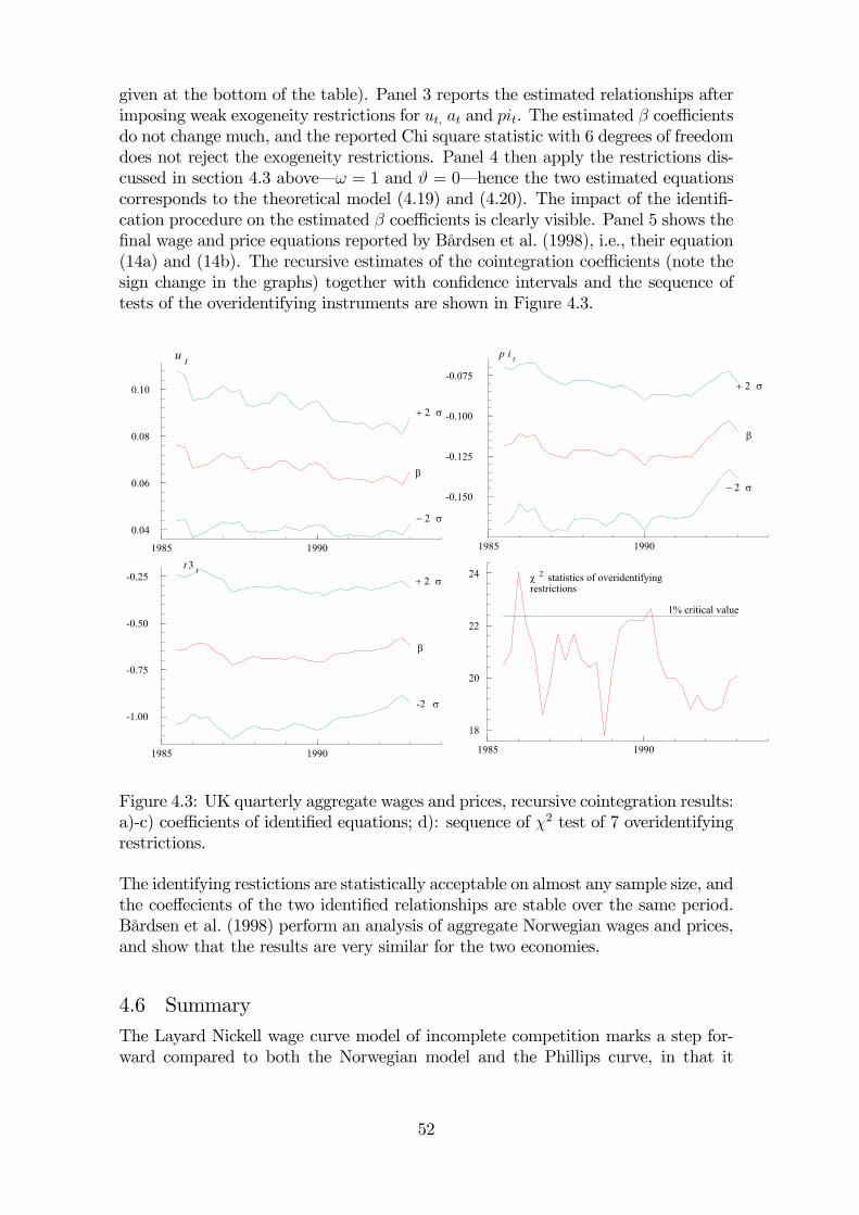
given at the bottom of the table). Panel 3 reports the estimated relationships afterimposing weak exogeneity restrictions for ut, at and pit. The estimated β coefficientsdo not change much, and the reported Chi square statistic with 6 degrees of freedomdoes not reject the exogeneity restrictions. Panel 4 then apply the restrictions dis-cussed in section 4.3 above–ω = 1 and ϑ = 0–hence the two estimated equationscorresponds to the theoretical model (4.19) and (4.20). The impact of the identifi-cation procedure on the estimated β coefficients is clearly visible. Panel 5 shows thefinal wage and price equations reported by Bårdsen et al. (1998), i.e., their equation(14a) and (14b). The recursive estimates of the cointegration coefficients (note thesign change in the graphs) together with confidence intervals and the sequence oftests of the overidentifying instruments are shown in Figure 4.3.
1985 1990
0.04
0.06
0.08
0.10
β
+ 2 σ
− 2 σ
u t
1985 1990
-0.150
-0.125
-0.100
-0.075+ 2 σ
− 2 σ
β
p i t
1985 1990
-1.00
-0.75
-0.50
-0.25 + 2 σ
β
-2 σ
t 3 t
1985 1990
18
20
22
24 χ 2 statistics of overidentifyingrestrictions
1% critical value
Figure 4.3: UK quarterly aggregate wages and prices, recursive cointegration results:a)-c) coefficients of identified equations; d): sequence of χ2 test of 7 overidentifyingrestrictions.
The identifying restictions are statistically acceptable on almost any sample size, andthe coeffecients of the two identified relationships are stable over the same period.Bårdsen et al. (1998) perform an analysis of aggregate Norwegian wages and prices,and show that the results are very similar for the two economies.
4.6 SummaryThe Layard Nickell wage curve model of incomplete competition marks a step for-ward compared to both the Norwegian model and the Phillips curve, in that it
52

combines formal models of wage bargaining and models of monopolistic price set-ting. Thus, compared to Aukrust’s model, the hypothesized cointegrating wage andprice cointegrating vectors are better founded in economic theory, and specific can-didates for explanatory variables flow naturally from the way the bargaining modelis formulated. We have shown that there are cases of substantive interest where theidentification problem pointed out by Manning (1993) are resolved, and have shownapplications with empirically stable and interpretable wage and price curves.
As a model of equilibrium unemployment, the framework is incomplete sinceonly the cointegrating part of the dynamic system is considered. To evaluate thenatural rate implication of the theory, which after all is much of the rationale forthe whole framework, a broader setting is required. That also defines the theme ofthe next section.
53
5 Wage-price dynamics
The open economy Phillips curve and the ICM appear to be positioned at oppositeends of a scale, with a simple dynamic model at the one end, and an economicallymore advanced but essentially static system at the other. In this section we presenta model of wage and price dynamics that contains the Phillips curve and the wagecurve as special cases, building on the analyses in Kolsrud and Nymoen (1998) andBårdsen and Nymoen (2003).
Section 5.1 presents the basic set of equations, and defines the concepts of staticand dynamic homogeneity and their relationships to nominal rigidity and absence ofneutrality to nominal shocks. Section 5.2 defines the asymptotically stable solutionof the system, and section 5.3 discusses some important economic implications ofthe conditional wage-price model as well as special cases that are of substantiveinterest (e.g., the no wedge case, and a small open economy interpretation, akinto the Norwegian model of inflation). The comparison with the ICM is drawnin section 5.4, while section 5.5 covers the Phillips curve case. Section 5.6 thengives an overview of the existing evidence in support of the restrictions that definesthe two natural rate models. Since we find that the evidence of the respectiveNAIRU restrictions are at best flimsy, we expect that endeavours to estimate a timevarying NAIRU run the danger of misrepresenting time varying coefficients of e.g.,wage equations as changes in structural features of the economy, and section 3.4substantiate that claim for the four main Nordic countries.
In brief, the natural rate thesis that stability of inflation is tantamount tohaving the rate of unemployment converging to a natural rate, is refuted both the-oretically and empirically in this section. Section 5.8 therefore sketch an modelfor inflation and unemployment dynamics that is consistent with the evidence andestimate the system for the Norwegian data set that is used throughout.
5.1 Nominal rigidity and equilibrium correctionThe understanding that conflict is an important aspect to take into account whenmodelling inflation in industrialized economies goes back at least to Rowthorn(1977), and has appeared frequently in models of the wage-price spiral, for exampleBlanchard (1987).35 In Rowthorn’s formulation, a distinction is drawn between thenegotiated profit share, corresponding to (1−wb
q,t − at) in equation (4.10), and thetarget profit share, i.e., (1− wf
q,t − at) in (4.13). If these shares are identical, thereis no conflict between the two levels of decision making (wage bargaining and firm’sunilateral pricing policy), and no inflation impetus.36 But if they are different, thereis conflict and inflation results as firms adjust prices unilaterally to rectify. In ourmodel, not only prices but also wages are allowed to change between two (central)bargaining rounds. This adds realism to the model, since even in countries likeNorway and Sweden, with strong traditions for centralized wage settlements, wage
35Norwegian economists know such models as ‘Haavelmo’s conflict model of inflation’, seeQvigstad (1975),36Haavelmo formulated his model, perhaps less deliberately, in terms of two separate target real
wage rates (again corresponding to wb and wf of the previous chapter) for workers and firms, butthe implications for inflation are the same as in Rowthorn’s model.
54
increases that are locally determined regularly end up with accounting for a signif-icant share of the total annual wage growth (i.e. so called wage drift, see Rødsethand Holden (1990) and Holden (1990)).
The model is also closely related to Sargan (1964), (1980) in that the dif-ference equations are written in equilibrium correction form, with nominal wageand price changes reacting to past disequilibria in wage formation and in price set-ting. In correspondence with the previous section, we assume that wages, prices andproductivity are I(1) variables, and that equations (4.11) and (4.14) are two coin-tegrating relationships. Cointegration implies equilibrium correction, so we specifythe following equations for wage and price growth:
(5.1)∆wt = θw(w
bq,t−1 − wq,t−1) + ψwp∆pt + ψwq∆qt − ϕut−1 + cw + εw,t,
0 ≤ ψwp + ψwq ≤ 1, ϕ ≥ 0, θw ≥ 0.and
(5.2)∆qt = −θq(wf
q,t−1 − wq,t−1) + ψqw∆wt + ψqi∆pit − ςut−1 + cq + εq,t,
0 ≤ ψqw + ψqi ≤ 1, , 0 ≤ θq, ς ≥ 0.εw,t and εq,t are assumed to be uncorrelated white noise processes. The equationsfor wb
q,t−1 and wfq,t−1 found in the previous section. Hence, for the wage side of
inflation process, equations (4.10) and (5.1) yield
(5.3)∆wt = kw + ψwp∆pt + ψwq∆qt − µwut−1
+θwωpq,t−1 − θwwq,t−1 + θwιat−1 + εw,t,
where kw = (cw + θwmb). In equation (5.3), the coefficient of the rate of unemploy-ment µw is defined by
(5.4) µw = θw (when θw < 0 ) or µw = ϕ ( when θw = 0).
which may seem cumbersome at first sight, but is required to secure internal con-sistency: Note that if the nominal wage rate is adjusting towards the long run wagecurve, θw < 0, the only logical value of for ϕ in (5.1) is zero, since ut−1 is already con-tained in the equation, with coefficient θw . Conversely, if θw = 0, it is neverthelesspossible that there is a wage Phillips curve relationship, hence µw = ϕ ≥ 0 in thiscase. In equation (5.3), long-run price homogeneity is ensured by the two laggedlevel-terms–the wedge pq,t−1 ≡ (p− q)t−1 and the real wage wq,t−1 ≡ (w − q)t−1.
For producer prices, equations (4.13) and (5.2) yield a dynamic equation ofthe cost mark-up type:
(5.5) ∆qt = kq + ψqw∆wt + ψqi∆pit − µqut−1 + θqwq,t−1 − θqat−1 + εq,t,
where kq = (cq − θqmf) and
(5.6) µq = θqϑ or µq = ς.
The definition of µq reflects exactly the same considerations as just explained forwage setting.
55
In terms of economic interpretation (5.3) and (5.5) are consistent with wageand price staggering and asynchronization among firms’ price setting, see e.g., An-dersen (1994, Ch. 7). An underlying assumption is that firms presets nominal pricesprior to the period and then within the period meets the demand forthcoming atthis price (which exceeds marginal costs, as in section 4). Clearly, the long run pricehomogeneity embedded in (5.3) is joined by long run homogeneity with respect towage costs in (5.5). Thus we have overall long term nominal homogeneity as aa direct consequence specifying the cointegrating relationships in terms of relativeprices.37
In static models, nominal homogeneity is synonymous with neutrality of outputto changes in nominal variables since relative prices are unaffected see e.g. Andersen(1994). This property does not carry over to the dynamic wage and price system,since relative prices (e.g., wq,t) will be affected for several periods following a shift infor example the price of imports. In general, the model implies nominal rigidity alongwith long term nominal homogeneity. Thus, care must also be taken when writingdown the conditions that eventually remove nominal rigidity from the system. Forexample, the conditions of “dynamic homogeneity”, i.e., ψwp + ψwq = 1 and ψqw +ψqi = 1, do not eliminate nominal rigidity as an implied property, see section 5.3.2.Interestingly, there is a one-to-one relationship between nominal neutrality and thenatural rate property, and a set of sufficient conditions are given in section 5.4.First however, section 5.2 defines the asymptotically stable solution of the systemwith long term homogeneity (but without neutrality) and section 5.3 discusses someimportant implications.
5.2 Stability and steady stateWe want to investigate the dynamics of the wage-price system consisting of equations(5.3), (5.5), and the definition equation
(5.7) pt = φqt + (1− φ)pit, 0 < φ < 1.
Following Kolsrud and Nymoen (1998), the model can be rewritten in terms of theproduct real wage wq,t, and the real exchange rate
(5.8) piq,t = pit − qt.
In order to close the model, we make two additional assumptions:
1. ut follows a separate ARMA process with mean uss.
2. pit and at are random walks with drift.
The NAIRU thesis states that the rate of unemployment has to be at an appropriateequilibrium level if the rate of inflation is to be stable. Assumption 1. is made toinvestigate whether that thesis holds true for the present model: With no feed-back
37see Kolsrud and Nymoen (1998) for an explicit parameterization with nominal variables withlong run homogeneity imposed.
56
from wq,t and/or piq,t on the rate of unemployment there is no way that ut can serveas an equilibrating mechanism. If a steady state exists in spite of this the NAIRUthesis is rejected, even though the model incorporates both the ICM and the Phillipscurve as special cases.
Obviously, in a more comprehensive model of inflation we will relax assumption1 and treat ut as an endogenous variable, in the same manner as in the Phillips curvecase of section 3. In the context of the imperfectly competition model, that step ispostponed until section 5.8. Assumption 2 eliminates stabilizing adjustments thatmight take place via the nominal exchange rate and/or in productivity. In empiricalwork it is an important question whether it is valid to condition on e.g., importprices (in domestic currency), cf section 4.4 above for an empirical example of weakexogeneity of productivity with respect to the identified long run wage curve.
The reduced form equation for the product real wage wq,t is
(5.9)wq,t = δt + ξ∆pit + κwq,t−1 + λpiq,t−1 − ηut−1 + wq ,t,
0 ≤ ξ ≤ 1, 0 ≤ κ ≤ 1, 0 ≤ λ,
with disturbance term wq ,t, a linear combination of εw,t and εq,t, and coefficientswhich amalgamate the parameters of the structural equations:
(5.10)
δt = [(cw + θwmb + θwιat−1)(1− ψqw)−(cq − θqmf − θqat−1)(1− ψwq − ψwpφ)]/χ
ξ = [ψwp(1− ψqw)(1− φ)− ψqi(1− ψwq − ψwpφ)]/χ,
λ = θwω(1− ψqw)(1− φ)/χ,
κ = 1− £θw(1− ψqw) + θq(1− ψwq − ψwpφ)¤/χ,
η = [µw(1− ψqw)− µq(1− ψwq − ψwpφ)]/χ.
The denominator of the expressions in (5.10) is given by
(5.11) χ = (1− ψqw(ψwq + ψwpφ)).
The corresponding reduced form equation for the real exchange rate piq,t can bewritten as
(5.12)piq,t = −dt + e∆pit − k wq,t−1 + l piq,t−1 + nut−1 + piq ,t,
0 ≤ e ≤ 1, l ≤ 1, 0 ≤ n,
where the parameters are given by
(5.13)
dt = [(cq − θqmf − θqat−1) + (cw + θwmb + θwιat−1)ψqw]/χ,
e = 1− [ψqwψwp(1− φ)− ψqi]/χ,
l = 1− £ψqwθwω(1− φ)/χ¤,
k = (θq − ψqwθw)/χ,
n = (µwψqw + µq)/χ.
Equations (5.9) and (5.12) constitute a system of first-order difference equations thatdetermines the real wage wq,t and the real exchange rate piq,t at each point in time.
57
As usual in dynamic economics we consider the deterministic system, correspondingto a hypothetical situation in which all shocks εw,t are εq,t (and thus wq ,t and piq,t)are set equal to zero. Once we have obtained the solutions for wq,t and piq,t, thetime paths for ∆wt, ∆pt and ∆qt can be found by backward substitution.
The roots of the characteristic equation of system are given by
(5.14) r =1
2
h(κ+ l)±
p(κ− l)2 − 4kλ
i,
hence the system has a unit-root whenever kλ = 0 and either κ = 1 or l = 1. Using(5.10) and (5.13), we conclude that the wage-price system has both its roots insidethe unit circle unless one or more of the following conditions hold:
θwω = 0,(5.15)
θw = θq = 0,(5.16)
ψqw(1− ψqw) = θq = 0.(5.17)
Based on (5.15)-(5.17), we can formulate a set of sufficient conditions for stableroots, namely
(5.18) θw > 0 and θq > 0 and ω > 0 and ψqw < 1.
The first two conditions represent equilibrium correction of wages and prices withrespect to deviations from the wage curve and the long run price setting schedule.The third condition states that there is a long run wedge effect in wage setting.Finally, a particular form of dynamic homogeneity is precluded by the fourth con-dition: a one point increase in the rate of wage growth, must lead to less than onepoint increase in the rate of price growth. Note that the fourth condition is muchmore restrictive than dynamic homogeneity in general which would be ψqw+ψqi = 1and ψwp + ψwq = 1. Dynamic homogeneity, in this usual sense is fully consistentwith a stable steady state.
5.3 The stable solution of the conditional wage-price systemIf the sufficient condition in (5.18) hold, we obtain a dynamic equilibrium–the“tug of war” between workers and firms reaches a stalemate. The system is stablein the sense that, if all stochastic shocks are switched-off, piq,t → piq,ss(t) andwq,t → wq,ss(t), where piq,ss(t) and wq,ss(t) denote the deterministic steady stategrowth paths of the real exchange rate and the product real wage. The steady stategrowth paths are independent of the historically determined initial conditions piq,0and wq,0 but depend on the steady state growth rate of import prices (gpi), of themean of ut denoted uss, and of the expected time path of productivity:
wq,ss(t) = ξ0gpi + η0uss + ga(t− 1)− δ0,(5.19)
piq,ss(t) = e0gpi + n0uss +1− ι
ω(1− φ)ga(t− 1)− d0,(5.20)
58
where ga is the drift parameter of productivity.38 The coefficients of the two steadystate paths in (5.19) and (5.20) are given by (5.21):
(5.21)
ξ0 = (1− ψqw − ψqi)/θq,
η0 = µq/θq,
δ0 = (cq − θqmf)/θq + coeff × ga,
e0 = [θq(1− ψwq − ψwp) + θw(1− ψqw)]/θwθqω(1− φ),
n0 = (θqµw + θwµq)/θwθqω(1− φ),
d0 = [θq(cw + θwmb) + θw(cq − θqmf)] /θwθqω(1− φ) + coeff × ga,
One interesting aspect of equations (5.19) and (5.20) is that they represent formal-izations and generalizations of the main course theory of section 2. In the currentmodel, domestic firms adjust their prices in response to the evolution of domesticcosts and foreign prices, they do not simply take world prices as given. In otherwords, the one-way causation of Aukrust’s model has been replaced by a wage-pricespiral. The impact of this generalization is clearly seen in (5.19) which states thatthe trend growth of productivity ga(t−1) traces out a main course, not for the nom-inal wage level as in figure 2.1, but for the real wage level. It is also consistent withAukrust’s ideas that the steady state of the wage share: wsss(t) ≡ wq,s(t)− ass(t),is without trend, i.e.,
(5.22) wsss = ξ0π + η0uss − δ0
but that it can change due to for example a deterministic shift in the long run meanof the rate of unemployment.
According to equation (5.20) it is seen that the real exchange rate in generalalso depends on the productivity trend. Thus, if ι < 1 in the long run wage equation(4.10) the model predicts continuing depreciation in real terms. Conversely, if ι = 1the steady state path of the real exchange rate is without a deterministic trend. Notethat sections 4.4 and 4.5 showed results for two data sets, where ι = 1 appeared tobe a valid parameter restriction.
Along the steady state growth path, with ∆uss = 0, the two rates of changeof real wages and the real exchange rate are given by:
∆wq,ss = ∆wss −∆qss = ga
∆piq,ss = ∆piss −∆qss =1− ι
ω(1− φ)ga.
Using these two equations, together with (5.7)
∆pss = φ∆qss + (1− φ)gpi
38Implicitly, the initial value a0 of productivity is set to zero.
59
we obtain
∆wss = gpi + ga(5.23)
∆qss = gpi − 1− ι
ω(1− φ)ga(5.24)
∆pss = gpi − φ(1− ι)
ω(1− φ)ga(5.25)
It is interesting to note that equation (5.23) is fully consistent with the Norwegianmodel of inflation of section 2.3. However, the existence of a steady state was merelypostulated in that section. The present analysis improves on that, since the steadyis derived from set of difference equations that includes wage bargaining theory andequilibrium correction dynamics. (5.24) and (5.25) show that the general solutionimplies a wedge between domestic and foreign inflation. However, in the case ofι = 1 (wage earners benefit fully in the long term from productivity gains), weobtain the standard open economy result that the steady state rate of inflation isequal to the rate of inflation abroad.
What does the model tell us about the status of the NAIRU? A succinctsummary of the thesis is given by Layard et al. (1994):
Only if the real wage (W/P ) desired by wage-setters is the same asthat desired by price-setters will inflation be stable. And the variablethat bring about this consistency is the level of unemployment39
Compare this to the equilibrium consisting of ut = uss, and wq,ss and piq,ss given by(5.19) and (5.20) above: Clearly, inflation is stable, since (5.23)-(5.25) is implied,even though uss is determined “from outside”, and is not determined by the wageand price setting equations of the model. Hence, the (emphasized) second sentencein the quotation is not supported by the steady state. In other words, it is notnecessary that uss corresponds to uw in equation (4.7) in section 4) for inflationto be stable. This contradiction of the quotation occurs in spite of the model’scloseness to the ICM, i.e., their wage and price setting schedules appear crucially inour model as cointegration relationships.
In sections 5.4 and 5.5 below, we return to the NAIRU issue. We show therethat both the wage curve and Phillips curve versions of the NAIRU are special casesof the model formulated above. But first, we need to discuss several importantspecial cases of wage-price dynamics.
5.3.1 Cointegration, long run multipliers and the steady state
There is a correspondence between the elasticities in the equations that describe thesteady state growth paths and the elasticities in the cointegrating relationships (4.11)and (4.14). However, care must be taken when mapping from one representation tothe other. For example, since much applied work pays more attention to wage setting(the bargaining model) than to price setting, it is often implied that the coefficientof unemployment in the estimated cointegrating wage equation also measures how
39Layard et al. (1994, p. 18), atuhors’ italics
60
much the steady state growth path of real wages changes as a result of a permanentshift in the rate of unemployment. In other words, the elasticity in the cointegratingequation is interpreted as the long run multiplier of real wages with respect to therate of unemployment. However, from (5.19) the general result (from the stablecase) is that the long run multiplier of the producer real wage wq is
∂wq
∂u= η0 = ϑ ≥ 0,
i.e., the elasticity of unemployment in the long term price setting equation (4.13),not the one in the wage-curve (4.11).
Moreover, long run multipliers are not invariant to the choice of deflator. Thus,if we instead consider the long run multiplier of the consumer real wage w − p, weobtain
∂(w − p)
∂u=
·ϑ(1− 1
ω)−
¸≤ 0.
Comparing the multipliers for the two definitions of the real wage, it is evident thatit is only the multiplier of the consumer real wage curve that has the conventionalnegative sign. However, also ∂(w − p)/∂u is a function of the elasticities from bothcointegrating relationships (price and wage).
The one-to-one correspondence between the long run multiplier and the un-employment elasticity in the “wage-curve” (4.11) requires additional assumptions.Consider for example the case of ω = 1 and ϑ = 0, i.e., only costs of living (notproduct prices) play a role in wage bargaining, and domestic firms practice normalcost pricing. As argued in section 4.3, this corresponds to the case of aggregatewage-price dynamics, and we obtain ∂wq
∂u= 0 and ∂(w−p)
∂u= − . Thus, the long run
multiplier of the consumer real wage is identical to the elasticity of unemploymentin the wage curve in this case.
5.3.2 Nominal rigidity despite dynamic homogeneity
At first sight, one might suspect that the result that uss is undetermined by the wageand price setting equations has to do with dynamic inhomogeneity, or “monetaryillusion”. For example, this is the case for the Phillips curve model where thesteady state rate of unemployment corresponds to the natural rate whenever thelong run Phillips curve is vertical, which in turn requires that dynamic homogeneityis fulfilled. Matters are different in the model in this section though. As explainedabove, the property of dynamic homogeneity requires that we impose ψqw+ψqi = 1in the equation representing price formation, and ψwq + ψwp = 1 in the dynamicwage curve. It is seen directly form (5.18) that the model is asymptotically stableeven when made subject to these two restrictions. Thus the equilibrium conditionedby the outside-determined level of unemployment, uss, does not depend on dynamicinhomogeneity. Hence, we have the interesting result that the two restrictions,ψqw + ψqi = 1 and ψwq + ψwp = 1 (dynamic homogeneity) do not remove nominalrigidity from the system: Even when no “monetary illusion” is present, real wagesand the real exchange rate are affected for several periods after a nominal shock.
61
The stable solution even applies to the case of ψqw = 1 (ψqi = 0), in whichcase the coefficients of the reduced form equation for wq,t reduce to
(5.26)
δt = −(cq − θqmf − θqat−1),
ξ = 0,
λ = 0,
κ = 1− θq,
η = −µq,while the coefficients (5.13) of the reduced form equation (5.12) for piq become
(5.27)
d = [(cq − θqmf − θqat−1) + (cw + θwmb + ιat−1)] /ψwp(1− φ),
e = 0,
l = 1− θwω/ψwp,
k = (θq − θw)/(ψwp(1− φ)),
n = (µw + µq)/(ψwp(1− φ)).
Since λ = 0 in (5.26), there is no effect of the real-exchange rate in the reducedform equation for real wages, hence the solution for real wages can be obtainedfrom equation (5.9) alone. Note also how all coefficients of the real wage equation(5.9) depend only on parameters from price-setting, whereas the competitivenessequation (5.12) still amalgamate parameters from both sides of the wage bargain,see the coefficients in (5.27).
The steady state is given by (5.19) and (5.20) as before. The expressions forη0 and n0 are unchanged, but ξ0 = e0 = 0 as a result of dynamic homogeneity, hencewe obtain the expected result that the steady state real exchange rate and the realwage are both unaffected by the rate of international inflation.
5.3.3 An important unstable solution: the “no wedge” case
Real wage resistance is an inherent aspect of the stable solution, as θwω 6= 0 is one ofthe conditions for the stability of the price-wage system, cf equation (5.15). However,as we have discussed above, the existence or otherwise of wedge effects remainsunsettled, both theoretically and empirically, and it is of interest to investigate thebehaviour of the system in the absence of real wage resistance, i.e. θwω = 0 due toω = 0.
Inspection of (5.9) and (5.12) shows that in this case, the system partitionsinto a stable real wage equation
(5.28) wq,t = δt + ξ∆pit + κwq,t−1 − ηut−1,
and an unstable equation for the real exchange rate
(5.29) ∆piq,t = −dt + e∆pit − kwq,t−1 + nut−1.
Thus, in the same way as in the stable case of ω > 0, the real wage follows astationary autoregressive process around the productivity trend which is included in
62
δt. However, from (5.29), the real exchange rate is seen to follow a unit-root process,albeit with wq,t−1, ut−1 and a (suppressed) disturbance term as I(0) variables on theright hand side. 40
The steady state real wage path is given by:
(5.30) wq,ss(t) =δt
(1− κ)+
ξ
(1− κ)gpi − η
(1− κ)uss.
Unlike the real wage given by (5.19) above, the coefficients of the long run real wagein (5.30) contains parameters from both sides of the bargain, not only price setting.The expression for the long run multiplier with respect to the unemployment rate,∂wq,ss/∂uss, shows interesting differences from the stable case in section 5.3:
∂wq,ss
∂uss= − [ θw(1− ψqw)− θqϑ(1− ψwq − ψwpφ)]£
θw(1− ψqw) + θq(1− ψwq − ψwpφ)¤
The multiplier is now a weighted sum of the two coefficients (wage curve) and ϑ(price setting). With normal cost pricing ϑ = 0, the long run multiplier is seen tobe negative.
The long-run elasticity of wq,ss with respect to productivity becomes
∂wq,ss
∂a=
ι+θqθw
1− ψwq − ψwpφ
1− ψqw
1 +θqθw
1− ψwq − ψwpφ
1− ψqw
.
hence, in the case of ι = 1 in the cointegrating wage equation, the long run multiplierimplies that the product real wage will increase by 1% as a result of a 1% permanentincrease in productivity. Thus, the steady state wage share is again without adeterministic trend.
The steady state rate of inflation in this the no-wedge case is obtained bysubstituting the solution for the real wage (5.30) back into the two equilibriumcorrection equations (5.3), imposing ω = 0, and (5.5), and then using the definitionof consumer prices in (4.9). The resulting steady-state rate of inflation can be showedto depend on the unemployment rate and on import price growth, i.e., ∆p 6= ∆pi inthe equilibrium associated with the “no wedge” case (ω = 0). Instead, the derivedlong-run Phillips curve is downward-sloping provided that η > 0.
Finally we note that, unlike the static wage curve of section 4, the “no wedge”restriction (ω = 0) in itself does not imply a supply side determined equilibriumrate of unemployment.41 The restrictions that are sufficient for the model to implya purely supply side determined equilibrium rate of unemployment is considered insection 5.4 below.
40Of course, if there is a long run effect of competitiveness on prices, i.e. (4.6) is extended by acompetitiveness term, ω = 0 is not sufficient to produce an unstable solution.41See e.g. (Layard et al., 1991, p. 391).
63
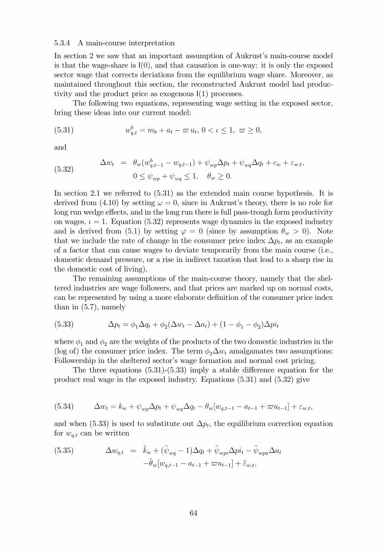
5.3.4 A main-course interpretation
In section 2 we saw that an important assumption of Aukrust’s main-course modelis that the wage-share is I(0), and that causation is one-way: it is only the exposedsector wage that corrects deviations from the equilibrium wage share. Moreover, asmaintained throughout this section, the reconstructed Aukrust model had produc-tivity and the product price as exogenous I(1) processes.
The following two equations, representing wage setting in the exposed sector,bring these ideas into our current model:
(5.31) wbq,t = mb + at − ut, 0 < ι ≤ 1, ≥ 0,
and
(5.32)∆wt = θw(w
bq,t−1 − wq,t−1) + ψwp∆pt + ψwq∆qt + cw + εw,t,
0 ≤ ψwp + ψwq ≤ 1, θw ≥ 0.
In section 2.1 we referred to (5.31) as the extended main course hypothesis. It isderived from (4.10) by setting ω = 0, since in Aukrust’s theory, there is no role forlong run wedge effects, and in the long run there is full pass-trough form productivityon wages, ι = 1. Equation (5.32) represents wage dynamics in the exposed industryand is derived from (5.1) by setting ϕ = 0 (since by assumption θw > 0). Notethat we include the rate of change in the consumer price index ∆pt, as an exampleof a factor that can cause wages to deviate temporarily from the main course (i.e.,domestic demand pressure, or a rise in indirect taxation that lead to a sharp rise inthe domestic cost of living).
The remaining assumptions of the main-course theory, namely that the shel-tered industries are wage followers, and that prices are marked up on normal costs,can be represented by using a more elaborate definition of the consumer price indexthan in (5.7), namely
(5.33) ∆pt = φ1∆qt + φ2(∆wt −∆at) + (1− φ1 − φ2)∆pit
where φ1 and φ2 are the weights of the products of the two domestic industries in the(log of) the consumer price index. The term φ2∆wt amalgamates two assumptions:Followership in the sheltered sector’s wage formation and normal cost pricing.
The three equations (5.31)-(5.33) imply a stable difference equation for theproduct real wage in the exposed industry. Equations (5.31) and (5.32) give
(5.34) ∆wt = kw + ψwp∆pt + ψwq∆qt − θw[wq,t−1 − at−1 + ut−1] + εw,t,
and when (5.33) is used to substitute out ∆pt, the equilibrium correction equationfor wq,t can be written
∆wq,t = kw + (ψwq − 1)∆qt + ψwpi∆pit − ψwpa∆at(5.35)
−θw[wq,t−1 − at−1 + ut−1] + εw,t,
64
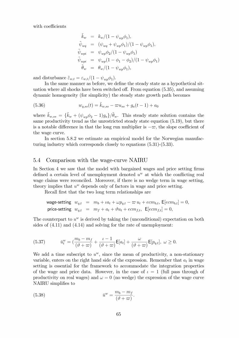
with coefficients
kw = kw/(1− ψwpφ1),
ψwq = (ψwq + ψwpφ1)/(1− ψwpφ1),
ψwpi = ψwpφ2/(1− ψwpφ1)
ψwpi = ψwp(1− φ1 − φ2)/(1− ψwpφ1)
θw = θw/(1− ψwpφ1),
and disturbance εw,t = εw,t/(1− ψwpφ1).In the same manner as before, we define the steady state as a hypothetical sit-
uation where all shocks have been switched off. From equation (5.35), and assumingdynamic homogeneity (for simplicity) the steady state growth path becomes
(5.36) wq,ss(t) = kw,ss − uss + ga(t− 1) + a0
where kw,ss = {kw + (ψwpφ2 − 1)ga}/θw. This steady state solution contains thesame productivity trend as the unrestricted steady state equation (5.19), but thereis a notable difference in that the long run multiplier is − , the slope coefficient ofthe wage curve.
In section 5.8.2 we estimate an empirical model for the Norwegian manufac-turing industry which corresponds closely to equations (5.31)-(5.33).
5.4 Comparison with the wage-curve NAIRUIn Section 4 we saw that the model with bargained wages and price setting firmsdefined a certain level of unemployment denoted uw at which the conflicting realwage claims were reconciled. Moreover, if there is no wedge term in wage setting,theory implies that uw depends only of factors in wage and price setting.
Recall first that the two long term relationships are
wage-setting wq,t = mb + ιat + ωpq,t − ut + ecmb,t, E[ecmb,t] = 0,
price-setting wq,t = mf + at + ϑut + ecmf,t, E[ecmf,t] = 0,
The counterpart to uw is derived by taking the (unconditional) expectation on bothsides of (4.11) and (4.14) and solving for the rate of unemployment:
(5.37) uwt = (mb −mf
(ϑ+ )+
ι− 1(ϑ+ )
E[at] +ω
(ϑ+ )E[pq,t], ω ≥ 0.
We add a time subscript to uw, since the mean of productivity, a non-stationaryvariable, enters on the right hand side of the expression. Remember that at in wagesetting is essential for the framework to accommodate the integration propertiesof the wage and price data. However, in the case of ι = 1 (full pass through ofproductivity on real wages) and ω = 0 (no wedge) the expression of the wage curveNAIRU simplifies to
(5.38) uw =mb −mf
(ϑ+ ).
65
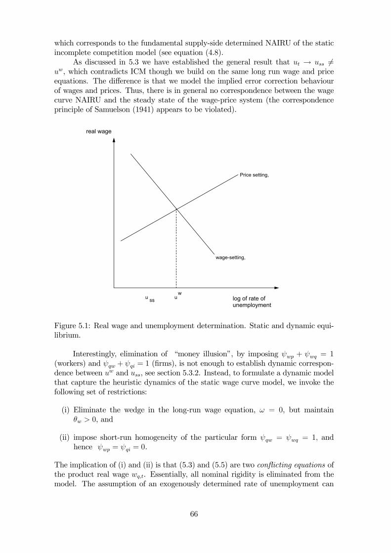
which corresponds to the fundamental supply-side determined NAIRU of the staticincomplete competition model (see equation (4.8).
As discussed in 5.3 we have established the general result that ut → uss 6=uw, which contradicts ICM though we build on the same long run wage and priceequations. The difference is that we model the implied error correction behaviourof wages and prices. Thus, there is in general no correspondence between the wagecurve NAIRU and the steady state of the wage-price system (the correspondenceprinciple of Samuelson (1941) appears to be violated).
real wage
log of rate ofunemployment
wage-setting,
Price setting,
uw
u ss
Figure 5.1: Real wage and unemployment determination. Static and dynamic equi-librium.
Interestingly, elimination of “money illusion”, by imposing ψwp + ψwq = 1(workers) and ψqw + ψqi = 1 (firms), is not enough to establish dynamic correspon-dence between uw and uss, see section 5.3.2. Instead, to formulate a dynamic modelthat capture the heuristic dynamics of the static wage curve model, we invoke thefollowing set of restrictions:
(i) Eliminate the wedge in the long-run wage equation, ω = 0, but maintainθw > 0, and
(ii) impose short-run homogeneity of the particular form ψqw = ψwq = 1, andhence ψwp = ψqi = 0.
The implication of (i) and (ii) is that (5.3) and (5.5) are two conflicting equations ofthe product real wage wq,t. Essentially, all nominal rigidity is eliminated from themodel. The assumption of an exogenously determined rate of unemployment can
66
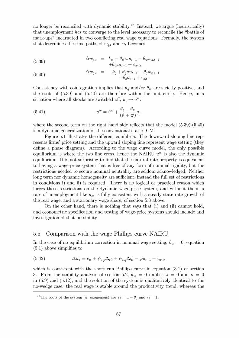
no longer be reconciled with dynamic stability.42 Instead, we argue (heuristically)that unemployment has to converge to the level necessary to reconcile the “battle ofmark-ups” incarnated in two conflicting real wage equations. Formally, the systemthat determines the time paths of wq,t and ut becomes
∆wq,t = kw − θw ut−1 − θwwq,t−1+θwιat−1 + εw,t,
(5.39)
∆wq,t = −kq + θqϑut−1 − θqwq,t−1+θqat−1 + εq,t.
(5.40)
Consistency with cointegration implies that θq and/or θw are strictly positive, andthe roots of (5.39) and (5.40) are therefore within the unit circle. Hence, in asituation where all shocks are switched off, ut → uw:
(5.41) uw = uw +θq − θw(ϑ+ )
ga
where the second term on the right hand side reflects that the model (5.39)-(5.40)is a dynamic generalization of the conventional static ICM.
Figure 5.1 illustrates the different equilibria. The downward sloping line rep-resents firms’ price setting and the upward sloping line represent wage setting (theydefine a phase diagram). According to the wage curve model, the only possibleequilibrium is where the two line cross, hence the NAIRU uw is also the dynamicequilibrium. It is not surprising to find that the natural rate property is equivalentto having a wage-price system that is free of any form of nominal rigidity, but therestrictions needed to secure nominal neutrality are seldom acknowledged: Neitherlong term nor dynamic homogeneity are sufficient, instead the full set of restrictionsin conditions i) and ii) is required. There is no logical or practical reason whichforces these restrictions on the dynamic wage-price system, and without them, arate of unemployment like uss is fully consistent with a steady state rate growth ofthe real wage, and a stationary wage share, cf section 5.3 above.
On the other hand, there is nothing that says that (i) and (ii) cannot hold,and econometric specification and testing of wage-price systems should include andinvestigation of that possibility
5.5 Comparison with the wage Phillips curve NAIRUIn the case of no equilibrium correction in nominal wage setting, θw = 0, equation(5.1) above simplifies to
(5.42) ∆wt = cw + ψwp∆pt + ψwq∆qt − ϕut−1 + εw,t,
which is consistent with the short run Phillips curve in equation (3.1) of section3. From the stability analysis of section 5.2, θw = 0 implies λ = 0 and κ = 0in (5.9) and (5.12), and the solution of the system is qualitatively identical to theno-wedge case: the real wage is stable around the productivity trend, whereas the
42The roots of the system (ut exogenous) are r1 = 1− θq and r2 = 1.
67
real exchange rate is unstable because of the unit root. Thus there is a paradox inthe sense that despite the open economy Phillips curve in (5.42), there is no impliedequilibrium rate of unemployment (uphil) of the form found in equation (3.10) insection 3. However, referring back to the Phillips curve system, it is clear that thatsystem involves an important extra assumption: Foreign prices were assumed totaken as given by domestic producers, which in the present model translates intoθq = ψqw = 0. Thus, restricting both wage and price setting by imposing
θw = θq = ψqw = 0,
is seen to imply two unit roots, and the system is now cast in terms of the twodifference variables ∆wq,t and ∆piq,t. Consequently, neither the real wage level northe real exchange rate are dynamically stable (even subtracting the productivitytrend). Heuristically, in order to re-establish a stable steady state for real wage, theassumption of a separate stationary model for ut must be replaced by something likeequation (3.2) in section 3, i.e., a separate equation for the rate of unemployment.43
5.6 Do estimated wage-price models support the NAIRU view ofequilibrium unemployment?
The analysis in this section has shown that there is no logical reason why dynamicstability of real wages and inflation should imply or “require” a supply side de-termined NAIRU. Conversely, by claiming that a derived (and estimated) NAIRUfrom an incomplete system of equations corresponds to the dynamic equilibriumlevel of unemployment in the economy, one invoke restrictions on the (unspecified)wage-price dynamics that may or may not hold empirically.
As we have seen, there are necessary conditions for correspondence that canbe tested from wage equations alone. This is fortunate, since there is virtually arange of studies that estimate wage models of the ICM type. Often the aim of thestudies have been to estimate the NAIRU, or at least to isolating its determinants.They represent a body of research evidence that can be re-interpreted using ourframework. While not claiming to be complete, section 5.6.1 paragraph aims tosummarize the evidence found in several econometric studies of (single equation)wage model.44 Section 5.6.2 then discuss in more detail the NAIRU implications ofa wage-price system estimated for UK aggregate data.
5.6.1 Empirical wage equations
Empirical models of Nordic manufacturing wage formation are reviewed and updatedin Rødseth and Nymoen (1999). Their results for Denmark, Finland, Norway andSweden strongly reject the Phillips-curve specification. The evidence against the
43Note that an identical line of reasoning starts from setting θq = 0 and leads to a price Phillipscurve NAIRU. This seems to give rise to an issue about logical (and empirical) indetermancy of theNAIRU, but influential papers like Gordon (1997) are not concerned with this, reporting insteaddifferent NAIRU estimates for different operational measures of inflation.44The last two sections of this chapter shows examples of full system anlyses, using Norwegian
and UK data.
68
Phillips curve hypothesis, θw = 0, is not confined to the Nordic countries, see e.g.,Grubb (1986) and Drèze and Bean (1990a) who analyze manufacturing wages for anumber of European economies.
Turning to the bargaining model, the main idea is that the NAIRU can bederived from the long-run real wage and price equations. If there is no wedge termin the wage equation, the NAIRU is independent of the real exchange rate. However,the above analysis shows that only subject to specific restrictions do the wage curveNAIRU correspond to the steady-state of the system. The Nordic study by Rødsethand Nymoen, while supporting that ω = 0, imply strong rejection of the NAIRUrestrictions on the dynamics. Results for other European countries give the sameimpression: For example, six out of ten country-studies surveyed by Drèze and Bean(1990a) do not imply a wage curve NAIRU, since they are not genuine product realwage equations: Either there is a wedge effect in the levels part of the equation(ω > 0), or the authors fail to impose ψwq = 1, ψwp = 0.
45
For the United Kingdom, there are several individual studies to choose from,some of which include a significant wedge effect, i.e. ω > 0, see for example Carruthand Oswald (1989) and Cromb (1993). In a comprehensive econometric study ofU.K. inflation, Rowlatt (1992) is able to impose dynamic homogeneity, ψwp+ψwq = 1in wage formation, but the NAIRU restriction ψwq = 1 is not supported by thedata.46 The work of Davies and Schøtt-Jensen (1994) contains similar evidence forseveral EU-countries. For the majority of the data sets, consumer price growthis found to be important alongside producer prices, and as we have showed thisis sufficient to question the logical validity of the claims made in the same study,namely that a steady state unemployment equilibrium is implied by the estimatedreal-wage equations.
OECD (1997c, Table 1.A.1) contains detailed wage equation results for 21countries. For 14 countries the reported specification is of the wage-curve type butthe necessary restrictions derived above on the short run dynamics are rejected.Phillips curve specifications are reported for the other seven countries, notably forthe United States which corroborates evidence in other studies, see Blanchard andKatz (1997) for a discussion.
This brief overview confirms the impression that on European data, the ev-idence supports a wage curve rather that a Phillips curve specification. However,in the light of the model framework of this section, the estimated wage curves donot support the identification of the implied NAIRUs with the equilibrium level ofunemployment.
45From (Drèze and Bean, 1990b, Table 1.4), and the country papers in Drèze and Bean (1990a)we extract that the equations for Austria, Britain and (at least for practical purposes) Germanyare “true” product real-wage equations. The equation for France is of the Phillips-curve type. Forthe other countries we have, using our own notation: Belgium and the Netherlands: Consumerreal-wage equations, i.e. ψwp = 1, ψwq = 0 and ω = 1. Denmark: ω = 1, ψwp = 0.24, ψwq = 0.76.Italy: ω = 0, ψwp = 0.2(1 − φ), ψwq = 0.8(1 − φ). United-States ω = 0.45(1 − φ), ψwq = 1,ψwp = 0. Spain: ω = 0.85 · 0.15, θw = 1, ψwp = ω, ψwq = 1− ω (The equation is static).46See (Rowlatt, 1992, Chapter 3.6).
69
5.6.2 Aggregate wage-price dynamics in the UK.
In section 4.5 we showed that, using aggregate wage and price data for the period1976(3)-1993(1), the following long term wage and price equations were identifiable,see table 4.3.
i) w = p+ a− t1− 0.065u+ constant(5.43)
ii) p = 0.89(w + t1− a) + 0.11pi+ 0.6t3 + constant .(5.44)
Next, consider the model in Table 5.1 which is by FIML. (5.43) and (5.44) areincorporated into the dynamic model as equilibrium-correction terms, and theirimportance is clearly shown. In addition to the equilibrium-correction term, wagesare driven by growth in consumer prices over the last two periods and by productivitygains. With a elasticity estimate of 0.66 and a standard error of 0.039, short-runhomogeneity is clearly rejected.
The negatively estimated coefficient for the change in the indirect tax-rate(∆t3t) is surprising at first sight. However, according to equation (5.44), consumerprices respond when the tax-rate is increased which in turn is passed on to wages.Hence, the net effect of a discretionary change in the indirect tax-rate on wages isestimated to be effectively zero in the short-run and positive in the intermediateand long-run. The effect of an increase in the payroll-tax rate is to reduce earnings,both in the short and long-run.
According to the second equation in Table 5.1, prices respond sharply (by0.96%) to a one percentage change in wage costs. Hence short-run homogeneity islikely to hold for prices. In addition to wage increases and equilibrium-correctionbehaviour, price inflation is seen to depend on the output gap, as captured by thevariable gap.
Finally, note that the two income policy-dummies, BONUS and IP4 aresignificant in both equations, albeit with different signs. Their impact in the firstequation is evidence of wage-raising incomes policies, and their reversed signs inthe price equation indicate that these effects were not completely anticipated byprice-setters.
The diagnostics reported at the bottom of Table 5.1 give evidence of a welldetermined model. In particular the insignificance of the overidentification χ2 showsthat the model encompasses the implied unrestricted reduced form, see Bårdsen et al.(1998) for evidence of recursive stability.
The significant equilibrium correction is consistent with previous cointegrationresults, and is clear cut evidence against a Phillips curve NAIRU, i.e., θq > 0 andθw > 0 in the theory model. As for the wage curve NAIRU, note that we have themodel formulation implies ω = 1 in the theory model ,rather than ω = 0 whichis one necessary requirement for correspondence between uw and uss. In addition,although the estimates suggest that dynamic homogeneity can be imposed in theprice equation, a similar restriction is statistically significant in the wage equation.
5.7 Econometric evaluation of Nordic structural employment esti-mates
While, early models treated the NAIRU as a quasi fixed parameter, cf the openeconomy Phillips curve NAIRU of section 3, the ICM framework provides the intel-
70
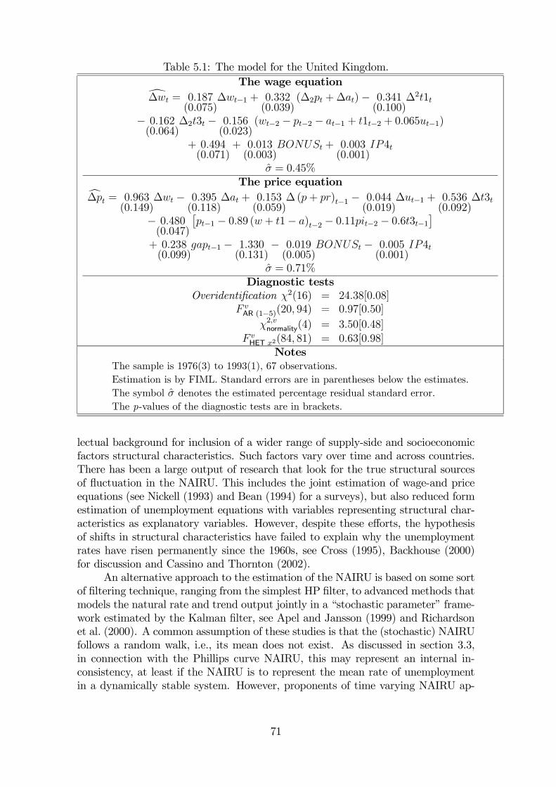
Table 5.1: The model for the United Kingdom.The wage equationd∆wt = 0.187
(0.075)∆wt−1 + 0.332
(0.039)(∆2pt +∆at)− 0.341
(0.100)∆2t1t
− 0.162(0.064)
∆2t3t − 0.156(0.023)
(wt−2 − pt−2 − at−1 + t1t−2 + 0.065ut−1)
+ 0.494(0.071)
+ 0.013(0.003)
BONUSt + 0.003(0.001)
IP4t
σ = 0.45%The price equationc∆pt = 0.963
(0.149)∆wt − 0.395
(0.118)∆at + 0.153
(0.059)∆ (p+ pr)t−1 − 0.044
(0.019)∆ut−1 + 0.536
(0.092)∆t3t
− 0.480(0.047)
£pt−1 − 0.89 (w + t1− a)t−2 − 0.11pit−2 − 0.6t3t−1
¤+ 0.238(0.099)
gapt−1 − 1.330(0.131)
− 0.019(0.005)
BONUSt − 0.005(0.001)
IP4t
σ = 0.71%Diagnostic tests
Overidentification χ2(16) = 24.38[0.08]F vAR (1−5)(20, 94) = 0.97[0.50]
χ2,vnormality(4) = 3.50[0.48]F vHET x2(84, 81) = 0.63[0.98]
NotesThe sample is 1976(3) to 1993(1), 67 observations.Estimation is by FIML. Standard errors are in parentheses below the estimates.The symbol σ denotes the estimated percentage residual standard error.The p-values of the diagnostic tests are in brackets.
lectual background for inclusion of a wider range of supply-side and socioeconomicfactors structural characteristics. Such factors vary over time and across countries.There has been a large output of research that look for the true structural sourcesof fluctuation in the NAIRU. This includes the joint estimation of wage-and priceequations (see Nickell (1993) and Bean (1994) for a surveys), but also reduced formestimation of unemployment equations with variables representing structural char-acteristics as explanatory variables. However, despite these efforts, the hypothesisof shifts in structural characteristics have failed to explain why the unemploymentrates have risen permanently since the 1960s, see Cross (1995), Backhouse (2000)for discussion and Cassino and Thornton (2002).
An alternative approach to the estimation of the NAIRU is based on some sortof filtering technique, ranging from the simplest HP filter, to advanced methods thatmodels the natural rate and trend output jointly in a “stochastic parameter” frame-work estimated by the Kalman filter, see Apel and Jansson (1999) and Richardsonet al. (2000). A common assumption of these studies is that the (stochastic) NAIRUfollows a random walk, i.e., its mean does not exist. As discussed in section 3.3,in connection with the Phillips curve NAIRU, this may represent an internal in-consistency, at least if the NAIRU is to represent the mean rate of unemploymentin a dynamically stable system. However, proponents of time varying NAIRU ap-
71
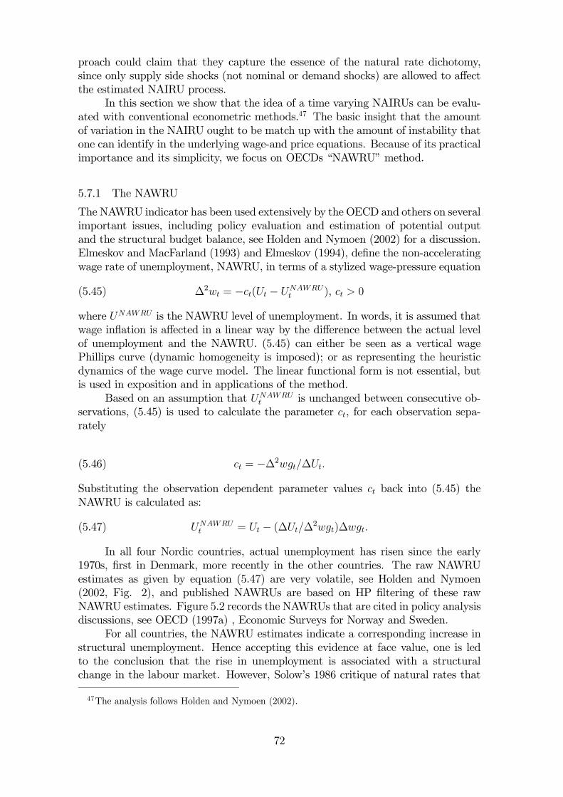
proach could claim that they capture the essence of the natural rate dichotomy,since only supply side shocks (not nominal or demand shocks) are allowed to affectthe estimated NAIRU process.
In this section we show that the idea of a time varying NAIRUs can be evalu-ated with conventional econometric methods.47 The basic insight that the amountof variation in the NAIRU ought to be match up with the amount of instability thatone can identify in the underlying wage-and price equations. Because of its practicalimportance and its simplicity, we focus on OECDs “NAWRU” method.
5.7.1 The NAWRU
The NAWRU indicator has been used extensively by the OECD and others on severalimportant issues, including policy evaluation and estimation of potential outputand the structural budget balance, see Holden and Nymoen (2002) for a discussion.Elmeskov and MacFarland (1993) and Elmeskov (1994), define the non-acceleratingwage rate of unemployment, NAWRU, in terms of a stylized wage-pressure equation
(5.45) ∆2wt = −ct(Ut − UNAWRUt ), ct > 0
where UNAWRU is the NAWRU level of unemployment. In words, it is assumed thatwage inflation is affected in a linear way by the difference between the actual levelof unemployment and the NAWRU. (5.45) can either be seen as a vertical wagePhillips curve (dynamic homogeneity is imposed); or as representing the heuristicdynamics of the wage curve model. The linear functional form is not essential, butis used in exposition and in applications of the method.
Based on an assumption that UNAWRUt is unchanged between consecutive ob-
servations, (5.45) is used to calculate the parameter ct, for each observation sepa-rately
(5.46) ct = −∆2wgt/∆Ut.
Substituting the observation dependent parameter values ct back into (5.45) theNAWRU is calculated as:
(5.47) UNAWRUt = Ut − (∆Ut/∆
2wgt)∆wgt.
In all four Nordic countries, actual unemployment has risen since the early1970s, first in Denmark, more recently in the other countries. The raw NAWRUestimates as given by equation (5.47) are very volatile, see Holden and Nymoen(2002, Fig. 2), and published NAWRUs are based on HP filtering of these rawNAWRU estimates. Figure 5.2 records the NAWRUs that are cited in policy analysisdiscussions, see OECD (1997a) , Economic Surveys for Norway and Sweden.
For all countries, the NAWRU estimates indicate a corresponding increase instructural unemployment. Hence accepting this evidence at face value, one is ledto the conclusion that the rise in unemployment is associated with a structuralchange in the labour market. However, Solow’s 1986 critique of natural rates that
47The analysis follows Holden and Nymoen (2002).
72
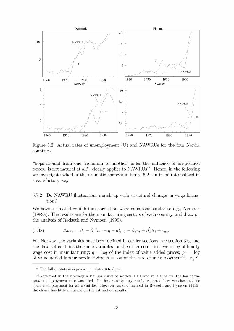
1960 1970 1980 1990
5
10
15
20
U
NAWRU
Finland
1960 1970 1980 1990
2
4
6
Norway
NAWRU
U
1960 1970 1980 1990
5
10
Denmark
NAWRU
U
1960 1970 1980 1990
2.5
5
7.5
10
NAWRU
U
Sweden
Figure 5.2: Actual rates of unemployment (U) and NAWRUs for the four Nordiccountries.
“hops around from one triennium to another under the influence of unspecifiedforces...is not natural at all”, clearly applies to NAWRUs48. Hence, in the followingwe investigate whether the dramatic changes in figure 5.2 can in be rationalized ina satisfactory way.
5.7.2 Do NAWRU fluctuations match up with structural changes in wage forma-tion?
We have estimated equilibrium correction wage equations similar to e.g., Nymoen(1989a). The results are for the manufacturing sectors of each country, and draw onthe analysis of Rødseth and Nymoen (1999).
(5.48) ∆wct = β0 − β1(wc− q − a)t−1 − β2ut + β0xXt + εwt.
For Norway, the variables have been defined in earlier sections, see section 3.6, andthe data set contains the same variables for the other countries: wc = log of hourlywage cost in manufacturing; q = log of the index of value added prices; pr = logof value added labour productivity; u = log of the rate of unemployment49. β
0xXt
48The full quotation is given in chapter 3.6 above.49Note that in the Norwegain Phillips curve of section XXX and in XX below, the log of the
total unemployment rate was used. In the cross country results reported here we chose to useopen unemployment for all countries. However, as documented in Rødseth and Nymoen (1999)the choice has little influence on the estimation results.
73
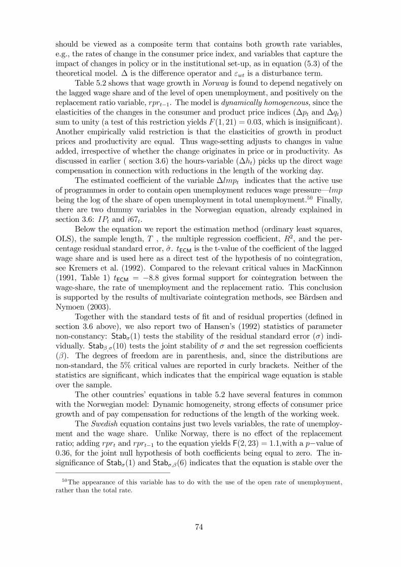
should be viewed as a composite term that contains both growth rate variables,e.g., the rates of change in the consumer price index, and variables that capture theimpact of changes in policy or in the institutional set-up, as in equation (5.3) of thetheoretical model. ∆ is the difference operator and εwt is a disturbance term.
Table 5.2 shows that wage growth in Norway is found to depend negatively onthe lagged wage share and of the level of open unemployment, and positively on thereplacement ratio variable, rprt−1. The model is dynamically homogeneous, since theelasticities of the changes in the consumer and product price indices (∆pt and ∆qt)sum to unity (a test of this restriction yields F (1, 21) = 0.03, which is insignificant).Another empirically valid restriction is that the elasticities of growth in productprices and productivity are equal. Thus wage-setting adjusts to changes in valueadded, irrespective of whether the change originates in price or in productivity. Asdiscussed in earlier ( section 3.6) the hours-variable (∆ht) picks up the direct wagecompensation in connection with reductions in the length of the working day.
The estimated coefficient of the variable ∆lmpt indicates that the active useof programmes in order to contain open unemployment reduces wage pressure–lmpbeing the log of the share of open unemployment in total unemployment.50 Finally,there are two dummy variables in the Norwegian equation, already explained insection 3.6: IPt and i67t.
Below the equation we report the estimation method (ordinary least squares,OLS), the sample length, T , the multiple regression coefficient, R2, and the per-centage residual standard error, σ. tECM is the t-value of the coefficient of the laggedwage share and is used here as a direct test of the hypothesis of no cointegration,see Kremers et al. (1992). Compared to the relevant critical values in MacKinnon(1991, Table 1) tECM = −8.8 gives formal support for cointegration between thewage-share, the rate of unemployment and the replacement ratio. This conclusionis supported by the results of multivariate cointegration methods, see Bårdsen andNymoen (2003).
Together with the standard tests of fit and of residual properties (defined insection 3.6 above), we also report two of Hansen’s (1992) statistics of parameternon-constancy: Stabσ(1) tests the stability of the residual standard error (σ) indi-vidually. Stabβ,σ(10) tests the joint stability of σ and the set regression coefficients(β). The degrees of freedom are in parenthesis, and, since the distributions arenon-standard, the 5% critical values are reported in curly brackets. Neither of thestatistics are significant, which indicates that the empirical wage equation is stableover the sample.
The other countries’ equations in table 5.2 have several features in commonwith the Norwegian model: Dynamic homogeneity, strong effects of consumer pricegrowth and of pay compensation for reductions of the length of the working week.
The Swedish equation contains just two levels variables, the rate of unemploy-ment and the wage share. Unlike Norway, there is no effect of the replacementratio; adding rprt and rprt−1 to the equation yields F(2, 23) = 1.1,with a p−value of0.36, for the joint null hypothesis of both coefficients being equal to zero. The in-significance of Stabσ(1) and Stabσ,β(6) indicates that the equation is stable over the
50The appearance of this variable has to do with the use of the open rate of unemployment,rather than the total rate.
74
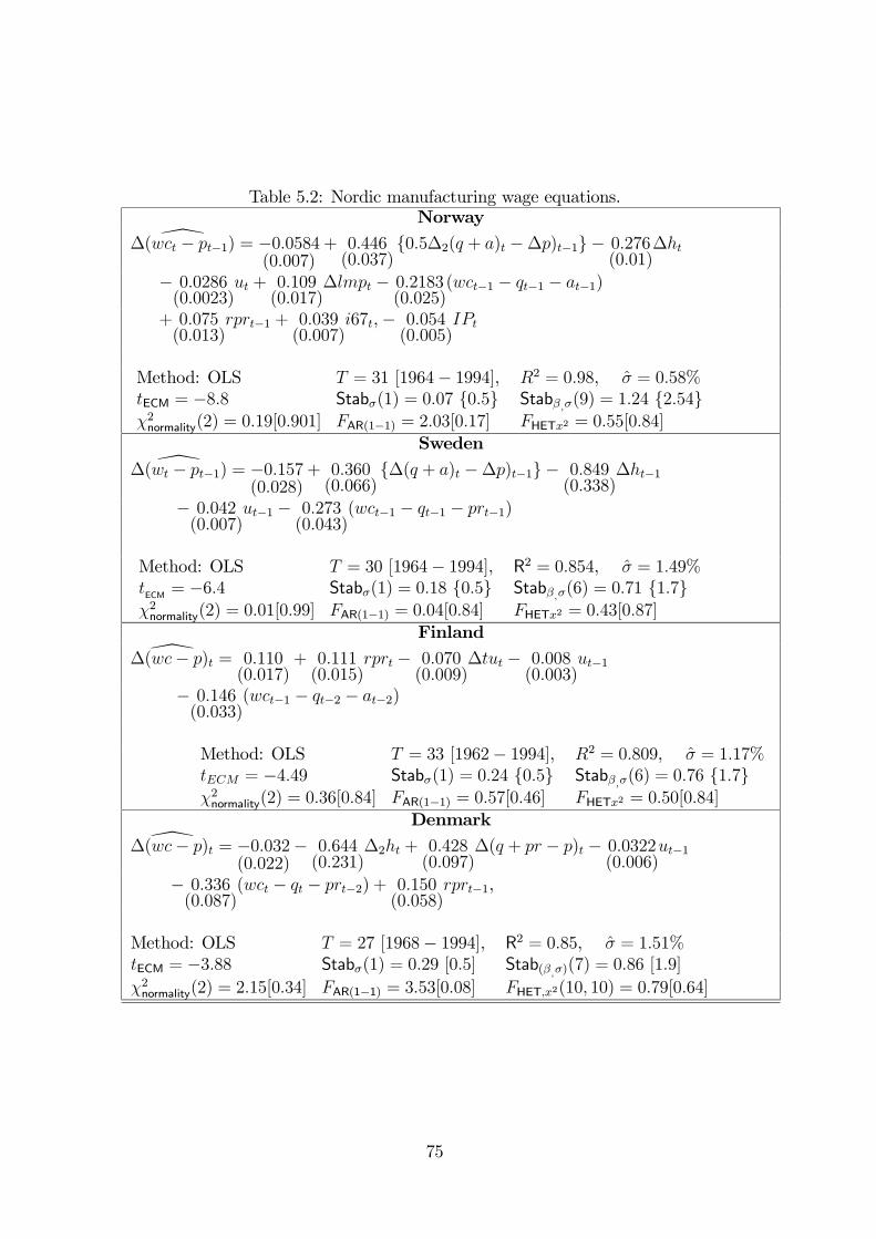
Table 5.2: Nordic manufacturing wage equations.Norway
\∆(wct − pt−1) = −0.0584(0.007)
+ 0.446(0.037)
{0.5∆2(q + a)t −∆p)t−1}− 0.276(0.01)
∆ht
− 0.0286(0.0023)
ut + 0.109(0.017)
∆lmpt − 0.2183(0.025)
(wct−1 − qt−1 − at−1)
+ 0.075(0.013)
rprt−1 + 0.039(0.007)
i67t,− 0.054(0.005)
IPt
Method: OLS T = 31 [1964− 1994], R2 = 0.98, σ = 0.58%tECM = −8.8 Stabσ(1) = 0.07 {0.5} Stabβ,σ(9) = 1.24 {2.54}χ2normality(2) = 0.19[0.901] FAR(1−1) = 2.03[0.17] FHETx2 = 0.55[0.84]
Sweden\∆(wt − pt−1) = −0.157
(0.028)+ 0.360(0.066)
{∆(q + a)t −∆p)t−1}− 0.849(0.338)
∆ht−1
− 0.042(0.007)
ut−1 − 0.273(0.043)
(wct−1 − qt−1 − prt−1)
Method: OLS T = 30 [1964− 1994], R2 = 0.854, σ = 1.49%tECM= −6.4 Stabσ(1) = 0.18 {0.5} Stabβ,σ(6) = 0.71 {1.7}
χ2normality(2) = 0.01[0.99] FAR(1−1) = 0.04[0.84] FHETx2 = 0.43[0.87]
Finland\∆(wc− p)t = 0.110
(0.017)+ 0.111(0.015)
rprt − 0.070(0.009)
∆tut − 0.008(0.003)
ut−1
− 0.146(0.033)
(wct−1 − qt−2 − at−2)
Method: OLS T = 33 [1962− 1994], R2 = 0.809, σ = 1.17%tECM = −4.49 Stabσ(1) = 0.24 {0.5} Stabβ,σ(6) = 0.76 {1.7}χ2normality(2) = 0.36[0.84] FAR(1−1) = 0.57[0.46] FHETx2 = 0.50[0.84]
Denmark\∆(wc− p)t = −0.032
(0.022)− 0.644(0.231)
∆2ht + 0.428(0.097)
∆(q + pr − p)t − 0.0322(0.006)
ut−1
− 0.336(0.087)
(wct − qt − prt−2) + 0.150(0.058)
rprt−1,
Method: OLS T = 27 [1968− 1994], R2 = 0.85, σ = 1.51%tECM = −3.88 Stabσ(1) = 0.29 [0.5] Stab(β,σ)(7) = 0.86 [1.9]χ2normality(2) = 2.15[0.34] FAR(1−1) = 3.53[0.08] FHET,x2(10, 10) = 0.79[0.64]
75
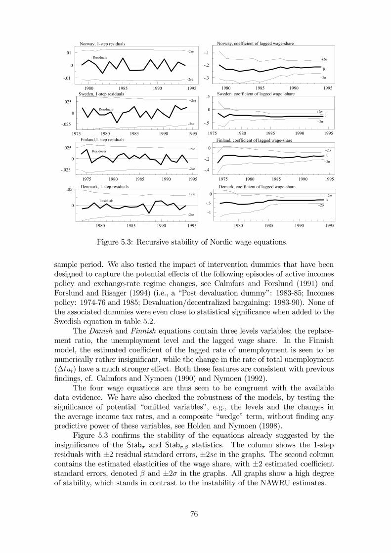
1980 1985 1990 1995
-.3
-.2
-.1
Norway, coefficient of lagged wage-share
1980 1985 1990 1995
-.01
0
.01Residuals
+2se
-2se
Norway, 1-step residuals
1975 1980 1985 1990 1995
-.025
0
.025
Sweden, 1-step residuals+2se
-2se
Residuals
1975 1980 1985 1990 1995
-.5
0
.5 Sweden. coefficient of lagged wage -share
+2σβ
−2σ
1975 1980 1985 1990 1995
-.025
0
.025Residuals
Finland,1-step residuals
+2se
-2se
1975 1980 1985 1990 1995
-.4
-.2
0
Finland, coefficient of lagged wage-share
+2σβ
−2σ
1980 1985 1990 1995
0
.05
Residuals
+2se
-2se
Denmark, 1-step residuals
1980 1985 1990 1995
-1
-.5
0
+2σ
−2σ
β
+2σβ
−2σ
Demark, coefficient of lagged wage-share
Figure 5.3: Recursive stability of Nordic wage equations.
sample period. We also tested the impact of intervention dummies that have beendesigned to capture the potential effects of the following episodes of active incomespolicy and exchange-rate regime changes, see Calmfors and Forslund (1991) andForslund and Risager (1994) (i.e., a “Post devaluation dummy”: 1983-85; Incomespolicy: 1974-76 and 1985; Devaluation/decentralized bargaining: 1983-90). None ofthe associated dummies were even close to statistical significance when added to theSwedish equation in table 5.2.
The Danish and Finnish equations contain three levels variables; the replace-ment ratio, the unemployment level and the lagged wage share. In the Finnishmodel, the estimated coefficient of the lagged rate of unemployment is seen to benumerically rather insignificant, while the change in the rate of total unemployment(∆tut) have a much stronger effect. Both these features are consistent with previousfindings, cf. Calmfors and Nymoen (1990) and Nymoen (1992).
The four wage equations are thus seen to be congruent with the availabledata evidence. We have also checked the robustness of the models, by testing thesignificance of potential “omitted variables”, e.g., the levels and the changes inthe average income tax rates, and a composite “wedge” term, without finding anypredictive power of these variables, see Holden and Nymoen (1998).
Figure 5.3 confirms the stability of the equations already suggested by theinsignificance of the Stabσ and Stabσ,β statistics. The column shows the 1-stepresiduals with ±2 residual standard errors, ±2se in the graphs. The second columncontains the estimated elasticities of the wage share, with ±2 estimated coefficientstandard errors, denoted β and ±2σ in the graphs. All graphs show a high degreeof stability, which stands in contrast to the instability of the NAWRU estimates.
76
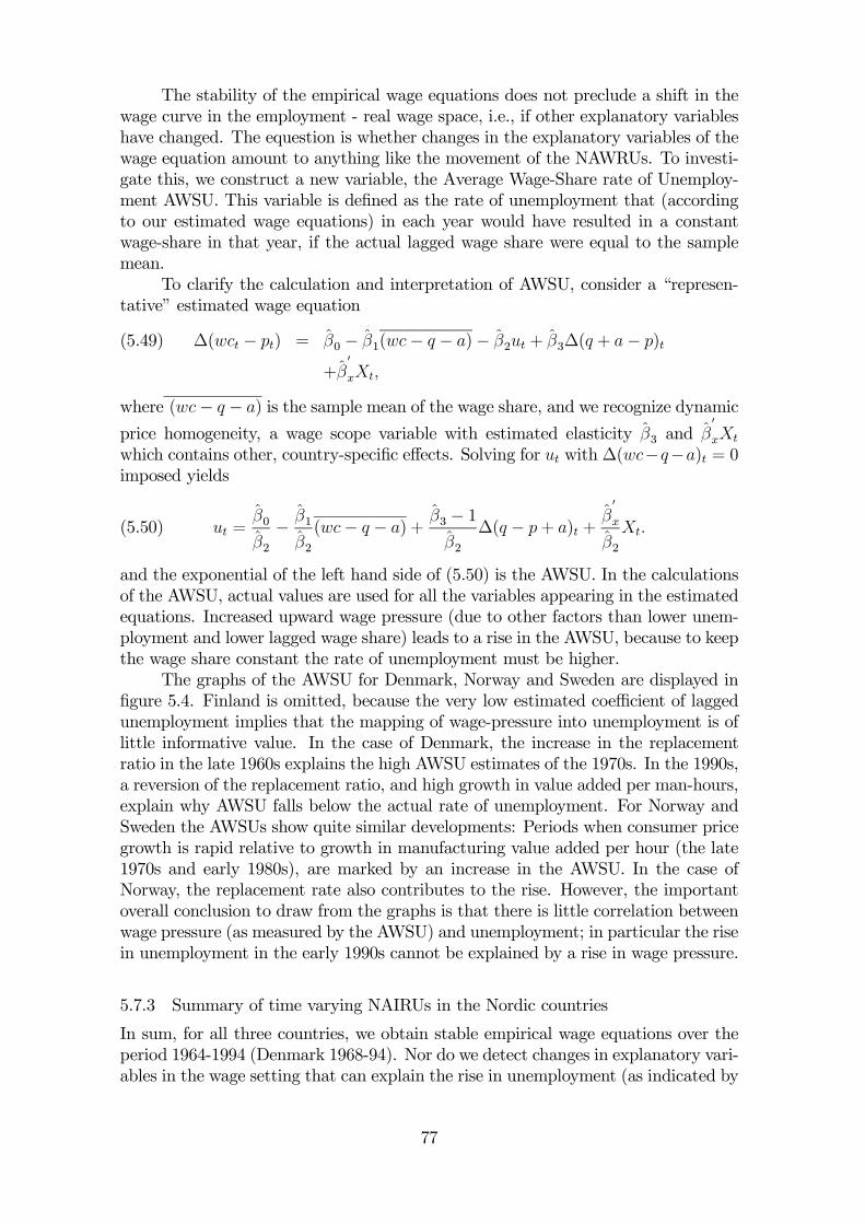
The stability of the empirical wage equations does not preclude a shift in thewage curve in the employment - real wage space, i.e., if other explanatory variableshave changed. The equestion is whether changes in the explanatory variables of thewage equation amount to anything like the movement of the NAWRUs. To investi-gate this, we construct a new variable, the Average Wage-Share rate of Unemploy-ment AWSU. This variable is defined as the rate of unemployment that (accordingto our estimated wage equations) in each year would have resulted in a constantwage-share in that year, if the actual lagged wage share were equal to the samplemean.
To clarify the calculation and interpretation of AWSU, consider a “represen-tative” estimated wage equation
∆(wct − pt) = β0 − β1(wc− q − a)− β2ut + β3∆(q + a− p)t(5.49)
+β0
xXt,
where (wc− q − a) is the sample mean of the wage share, and we recognize dynamic
price homogeneity, a wage scope variable with estimated elasticity β3 and β0
xXt
which contains other, country-specific effects. Solving for ut with ∆(wc−q−a)t = 0imposed yields
(5.50) ut =β0
β2− β1
β2(wc− q − a) +
β3 − 1β2
∆(q − p+ a)t +β0
x
β2Xt.
and the exponential of the left hand side of (5.50) is the AWSU. In the calculationsof the AWSU, actual values are used for all the variables appearing in the estimatedequations. Increased upward wage pressure (due to other factors than lower unem-ployment and lower lagged wage share) leads to a rise in the AWSU, because to keepthe wage share constant the rate of unemployment must be higher.
The graphs of the AWSU for Denmark, Norway and Sweden are displayed infigure 5.4. Finland is omitted, because the very low estimated coefficient of laggedunemployment implies that the mapping of wage-pressure into unemployment is oflittle informative value. In the case of Denmark, the increase in the replacementratio in the late 1960s explains the high AWSU estimates of the 1970s. In the 1990s,a reversion of the replacement ratio, and high growth in value added per man-hours,explain why AWSU falls below the actual rate of unemployment. For Norway andSweden the AWSUs show quite similar developments: Periods when consumer pricegrowth is rapid relative to growth in manufacturing value added per hour (the late1970s and early 1980s), are marked by an increase in the AWSU. In the case ofNorway, the replacement rate also contributes to the rise. However, the importantoverall conclusion to draw from the graphs is that there is little correlation betweenwage pressure (as measured by the AWSU) and unemployment; in particular the risein unemployment in the early 1990s cannot be explained by a rise in wage pressure.
5.7.3 Summary of time varying NAIRUs in the Nordic countries
In sum, for all three countries, we obtain stable empirical wage equations over theperiod 1964-1994 (Denmark 1968-94). Nor do we detect changes in explanatory vari-ables in the wage setting that can explain the rise in unemployment (as indicated by
77
1965 1970 1975 1980 1985 1990 1995
5
10AWSU
U
Denmark
1965 1970 1975 1980 1985 1990 1995
2.5
5
7.5
10 Norway
AWSU
U
AWSU
1965 1970 1975 1980 1985 1990 1995
2.5
5
7.5
Sweden
U
Figure 5.4: Unemployment and the Average Wage-Share rates of Unemployment(AWSU; see explanation in text).
absence of an increasing trend in the AWSU indicator in Figure 5.4).The instabilityof the NAWRU estimate appears to be an artefact of a misspecified underlying wageequation, and is not due to instability in the wage setting itself. Note also that theconclusion is not specific to the NAWRU but extends to other methods of estimatinga time varying NAIRU: As long as the premise of these estimations are that anysignificant changes in the NAIRU is due to changes in wage (or price) setting, theyalso have as a common implication that the conditional wage equations in table 5.2should be unstable. Since they are not, a class of models is seen to be inconsistentwith the evidence.
The results bring us back to the main question, of whether empirical macro-economic modelling should be based on the natural rate doctrine? The evidencepresented in this section more than suggest that there is a negative answer to thisquestion. Instead we might conclude that if the equilibrium level of unemploymentis going to be a strong attractor of actual unemployment, without displaying incred-ible jumps or unreasonably strong drift, the dichotomy between structural supplyside factors and demand side influences has to be given up. In the next section weoutline a framework that goes beyond the natural rate model.
5.8 Beyond the natural rate doctrine: Unemployment-inflation dy-namics
In this section we relax the assumption, made early in the section, of exogenouslydetermined unemployment which after all was made for a specific purpose: namely
78

for showing that under reasonable assumptions about price and wage setting, thereexist a steady state rate of inflation, and a steady state growth rates for real wagesfor a given long run mean of the rate of unemployment. Thus, the truism that asteady state requires that the rate of unemployment simultaneously converges tothe NAIRU has been refuted. Moreover, we have investigated special cases wherethe natural doctrine represents the only logically possible equilibrium, and havediscussed how the empirical relevance of those special cases can be asserted.
5.8.1 A complete system
(5.51)-(5.57) is a distilled version of an interdependent system for real-wages, thereal exchange rate and unemployment that we expect to encounter in practicalsituations.
∆wq,t = δt + ξ∆pit + (κ− 1)wq,t−1 + λpiq,t−1 − ηut−1 + εwq ,t,(5.51)
∆piq,t = −dt + e∆pit − k wq,t−1 + (l − 1) piq,t−1 + nut−1 + εpiq ,t,(5.52)
∆ut = βu0 − (1− βu1)ut−1 + βu2wq,t−1 + βu3at−1+(5.53)
+βu4piq,t−1 − βu5zut + εu,t.
∆pit = gpi + εpi,t(5.54)
∆qt = ∆pit −∆piq,t(5.55)
∆wt = ∆wq,t +∆qt(5.56)
∆pt = bp1(∆wt −∆at) + bp2∆pit + εp,t(5.57)
(5.51) and (5.52) are identical to equations (5.9) and (5.12) of section 5.1 and 5.2,where the coefficients were defined. Note that the two intercepts have time subscriptssince they include the (exogenous) labour productivity at, cf (5.10) and (5.13). Thetwo equations are the reduced forms of the theoretical model that combines wagebargaining and monopolistic price setting with equilibrium correction dynamics.Long run dynamic homogeneity is incorporated, but the system is characterized bynominal rigidity. Moreover, as explained above, not even dynamic homogeneity inwage and price setting is in general sufficient to remove nominal rigidity as a systemproperty.
A relationship equivalent to (5.53) was introduced already in section 3.2, inorder to close the open economy Phillips curve model. However there are two dif-ferences as a result of the more detailed modelling of wages and priced: First, sincethe real exchange rate is endogenous in the general model of wage price dynamics,we now include piq,t−1with non-negative coefficient (βu,4 ≥ 0).51 Second, since wemaintain the assumption about stationarity of the rate of unemployment (in theabsence of structural break), i.e., |βu1| < 1), we include at−1 unrestricted, in orderto balance the productivity effects on real wages and/or the real exchange rate. Inthe same way as in section on the Phillips curve system, zut represents a vectorconsisting of I(0) stochastic variables, as well as deterministic explanatory variables.
51The other elasticities in (5.53) are also non negative.
79
Equation (5.54) restates the assumption of random walk behavior of importprices made at the start of the section, and the following two equations are definitionsthat back out the nominal growth rates of the product price and nominal wage costs.The last equation of the system, (5.57), is a hybrid equation for the rate of inflationthat has normal cost pricing in the non-tradeables sector built into it.52
The essential difference from the wage-price model of section 5.1 is of courseequation (5.53) for the rate of unemployment. Unless βu2 = βu3 = 0, the stabilityanalysis of section 5.3 no longer applies, and it becomes impractical to map theconditions for stable roots back to the parameters. However, for estimated versionsof (5.51)-(5.57) the stability or otherwise is checked from the eigenvalues of theassociated companion matrix (as demonstrated in the next paragraph). Subject tostationarity, the steady state solution is easily obtained from (5.51)-(5.53) by setting∆wq,t = ga, ∆piq,t = 0, ∆uss = 0 and solving for wq,ss, piq,ss and uss. In general, allthree steady state variables becomes functions of the steady states of the variablesin the vector zu,t, the conditioning variables in the third unemployment equation, inparticular
uss = f(zu,ss).
Note that while the real wage is fundamentally influenced by productivity, ut ∼ I(0)implies that equilibrium unemployment uss is unaffected by the level of produc-tivity. Is this equilibrium rate of unemployment a ‘natural rate’? If we think ofthe economic interpretation of (5.53) this seems unlikely: (5.53) is a reduced formconsisting of labour supply, and the labour demand of private firms as well as ofgovernment employment. Thus, one can think of several factors in zu,t that stemfrom domestic demand, as well as from the foreign sector. At the end of the day,the justification of the specific terms included zu,ss and evaluation of the relativestrength of demand and supply side factors, must be made with with reference tothe institutional and historical characteristics of the data.
In the next section we give an empirical example of (5.51)-(5.57), and in thenext part of the book present operational macroeconomic models with a core wage-price model, and where (5.51) is replaced by a large system of equations describingoutput, labour demand and supply, domestic demand and financial markets.
5.8.2 Wage-price dynamics: Norwegian manufacturing
In this section we return to the manufacturing data set of section 3.6 (Phillips curve),and 4.4 (wage curve). In particular, we recapitulate the cointegration analysis ofsection 4.4:
1. A long run wage equation for the Norwegian manufacturing industry:
(5.58) wct − qt − at = − 0.065(0.081)
ut + 0.184(0.036)
rprt + ecmw,t,
i.e., equation (4.22) above. rprt is the log of the replacement ratio.
2. No wedge term in the wage curve cointegration relationship, (i.e., ω = 0).
52This equation is similar to (3.9) in the Phillips curve chapter. The only difference is that wenow let import prices represent imported inflation.
80
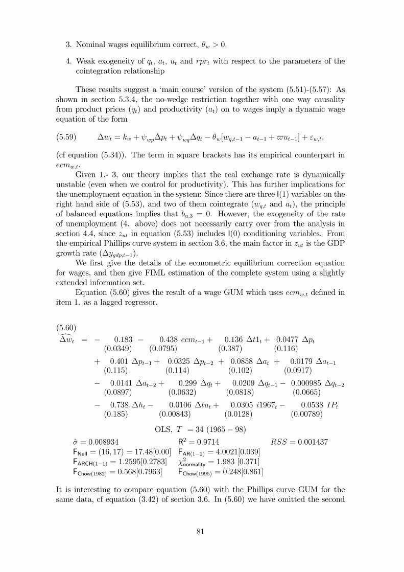
3. Nominal wages equilibrium correct, θw > 0.
4. Weak exogeneity of qt, at, ut and rprt with respect to the parameters of thecointegration relationship
These results suggest a ‘main course’ version of the system (5.51)-(5.57): Asshown in section 5.3.4, the no-wedge restriction together with one way causalityfrom product prices (qt) and productivity (at) on to wages imply a dynamic wageequation of the form
(5.59) ∆wt = kw + ψwp∆pt + ψwq∆qt − θw[wq,t−1 − at−1 + ut−1] + εw,t,
(cf equation (5.34)). The term in square brackets has its empirical counterpart inecmw,t.
Given 1.- 3, our theory implies that the real exchange rate is dynamicallyunstable (even when we control for productivity). This has further implications forthe unemployment equation in the system: Since there are three I(1) variables on theright hand side of (5.53), and two of them cointegrate (wq,t and at), the principleof balanced equations implies that bu,3 = 0. However, the exogeneity of the rateof unemployment (4. above) does not necessarily carry over from the analysis insection 4.4, since zut in equation (5.53) includes I(0) conditioning variables. Fromthe empirical Phillips curve system in section 3.6, the main factor in zut is the GDPgrowth rate (∆ygdp,t−1).
We first give the details of the econometric equilibrium correction equationfor wages, and then give FIML estimation of the complete system using a slightlyextended information set.
Equation (5.60) gives the result of a wage GUM which uses ecmw,t defined initem 1. as a lagged regressor.
d∆wt = − 0.183(0.0349)
− 0.438(0.0795)
ecmt−1 + 0.136(0.387)
∆t1t + 0.0477(0.116)
∆pt
+ 0.401(0.115)
∆pt−1 + 0.0325(0.114)
∆pt−2 + 0.0858(0.102)
∆at + 0.0179(0.0917)
∆at−1
− 0.0141(0.0897)
∆at−2 + 0.299(0.0632)
∆qt + 0.0209(0.0818)
∆qt−1 − 0.000985(0.0665)
∆qt−2
− 0.738(0.185)
∆ht − 0.0106(0.00843)
∆tut + 0.0305(0.0128)
i1967t − 0.0538(0.00789)
IPt
(5.60)
OLS, T = 34 (1965− 98)σ = 0.008934 R2 = 0.9714 RSS = 0.001437FNull = (16, 17) = 17.48[0.00] FAR(1−2) = 4.0021[0.039]FARCH(1−1) = 1.2595[0.2783] χ2normality = 1.983 [0.371]FChow(1982) = 0.568[0.7963] FChow(1995) = 0.248[0.861]
It is interesting to compare equation (5.60) with the Phillips curve GUM for thesame data, cf equation (3.42) of section 3.6. In (5.60) we have omitted the second
81
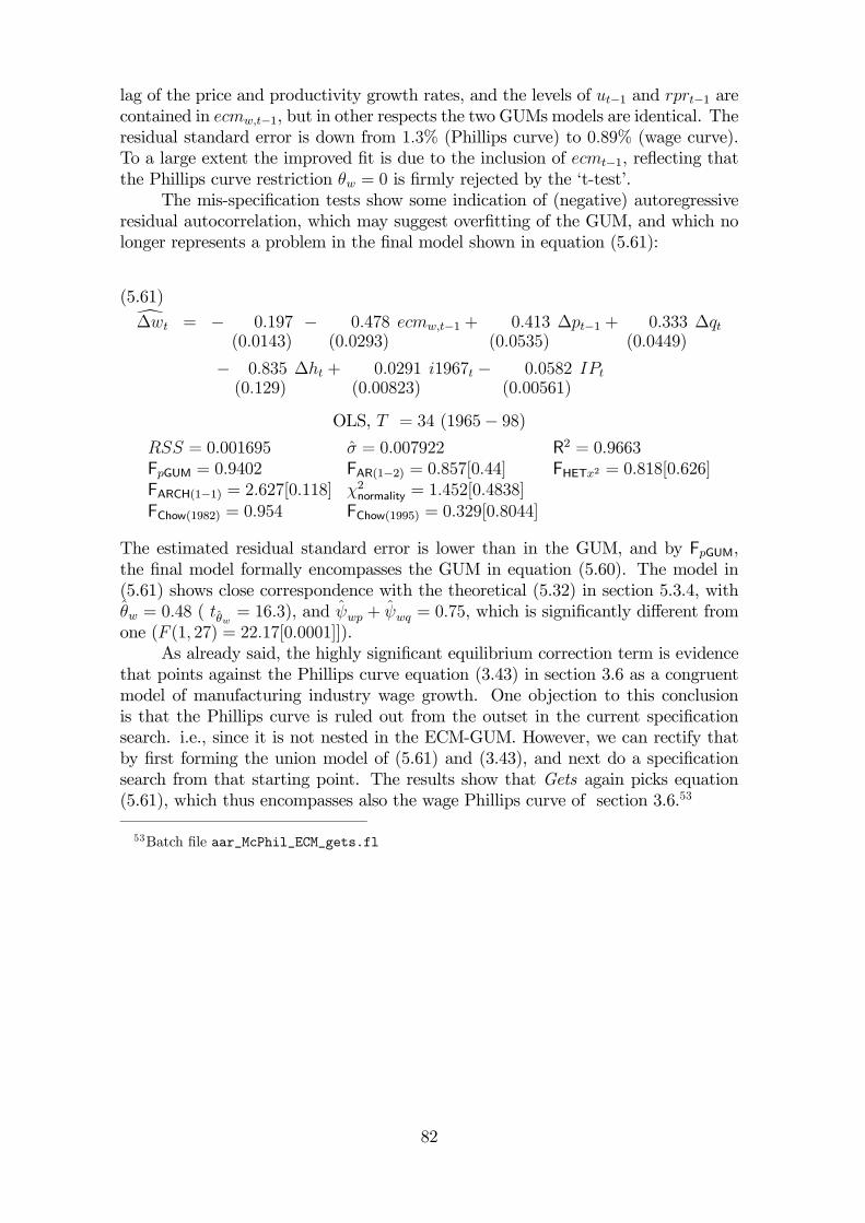
lag of the price and productivity growth rates, and the levels of ut−1 and rprt−1 arecontained in ecmw,t−1, but in other respects the two GUMs models are identical. Theresidual standard error is down from 1.3% (Phillips curve) to 0.89% (wage curve).To a large extent the improved fit is due to the inclusion of ecmt−1, reflecting thatthe Phillips curve restriction θw = 0 is firmly rejected by the ‘t-test’.
The mis-specification tests show some indication of (negative) autoregressiveresidual autocorrelation, which may suggest overfitting of the GUM, and which nolonger represents a problem in the final model shown in equation (5.61):
d∆wt = − 0.197(0.0143)
− 0.478(0.0293)
ecmw,t−1 + 0.413(0.0535)
∆pt−1 + 0.333(0.0449)
∆qt
− 0.835(0.129)
∆ht + 0.0291(0.00823)
i1967t − 0.0582(0.00561)
IPt
(5.61)
OLS, T = 34 (1965− 98)RSS = 0.001695 σ = 0.007922 R2 = 0.9663FpGUM = 0.9402 FAR(1−2) = 0.857[0.44] FHETx2 = 0.818[0.626]FARCH(1−1) = 2.627[0.118] χ2normality = 1.452[0.4838]FChow(1982) = 0.954 FChow(1995) = 0.329[0.8044]
The estimated residual standard error is lower than in the GUM, and by FpGUM,the final model formally encompasses the GUM in equation (5.60). The model in(5.61) shows close correspondence with the theoretical (5.32) in section 5.3.4, withθw = 0.48 ( tθw = 16.3), and ψwp + ψwq = 0.75, which is significantly different fromone (F (1, 27) = 22.17[0.0001]]).
As already said, the highly significant equilibrium correction term is evidencethat points against the Phillips curve equation (3.43) in section 3.6 as a congruentmodel of manufacturing industry wage growth. One objection to this conclusionis that the Phillips curve is ruled out from the outset in the current specificationsearch. i.e., since it is not nested in the ECM-GUM. However, we can rectify thatby first forming the union model of (5.61) and (3.43), and next do a specificationsearch from that starting point. The results show that Gets again picks equation(5.61), which thus encompasses also the wage Phillips curve of section 3.6.53
53Batch file aar_McPhil_ECM_gets.fl
82
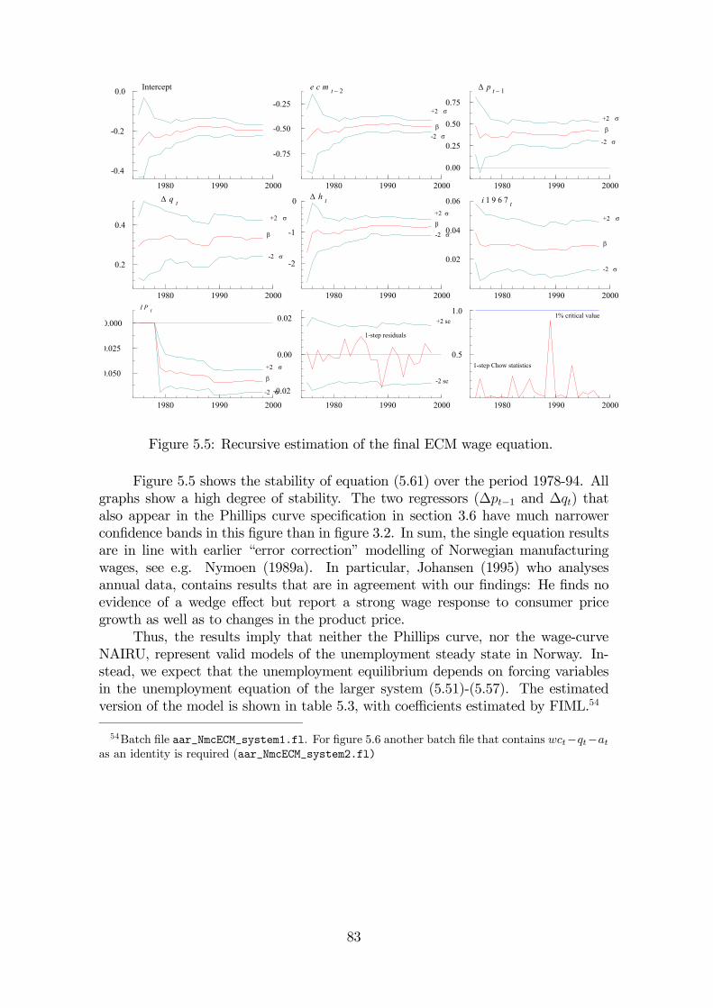
1980 1990 2000
-0.4
-0.2
0.0 Intercept
1980 1990 2000
-0.75
-0.50
-0.25
e c m t − 2
β
+2 σ
-2 σ
1980 1990 2000
0.00
0.25
0.50
0.75
∆ p t − 1
+2 σ
β
-2 σ
1980 1990 2000
0.2
0.4
∆ q t
-2 σ
+2 σ
β
1980 1990 2000
-2
-1
0 ∆ h t
+2 σ
β
-2 σ
1980 1990 2000
0.02
0.04
0.06 i 1 9 6 7 t
+2 σ
β
-2 σ
1980 1990 2000
0.050
0.025
0.000
I P t
+2 σ
β
-2 σ
1980 1990 2000
-0.02
0.00
0.02
1-step residuals
+2 se
-2 se
1980 1990 2000
0.5
1.0
1-step Chow statistics
1% critical value
Figure 5.5: Recursive estimation of the final ECM wage equation.
Figure 5.5 shows the stability of equation (5.61) over the period 1978-94. Allgraphs show a high degree of stability. The two regressors (∆pt−1 and ∆qt) thatalso appear in the Phillips curve specification in section 3.6 have much narrowerconfidence bands in this figure than in figure 3.2. In sum, the single equation resultsare in line with earlier “error correction” modelling of Norwegian manufacturingwages, see e.g. Nymoen (1989a). In particular, Johansen (1995) who analysesannual data, contains results that are in agreement with our findings: He finds noevidence of a wedge effect but report a strong wage response to consumer pricegrowth as well as to changes in the product price.
Thus, the results imply that neither the Phillips curve, nor the wage-curveNAIRU, represent valid models of the unemployment steady state in Norway. In-stead, we expect that the unemployment equilibrium depends on forcing variablesin the unemployment equation of the larger system (5.51)-(5.57). The estimatedversion of the model is shown in table 5.3, with coefficients estimated by FIML.54
54Batch file aar_NmcECM_system1.fl. For figure 5.6 another batch file that contains wct−qt−atas an identity is required (aar_NmcECM_system2.fl)
83
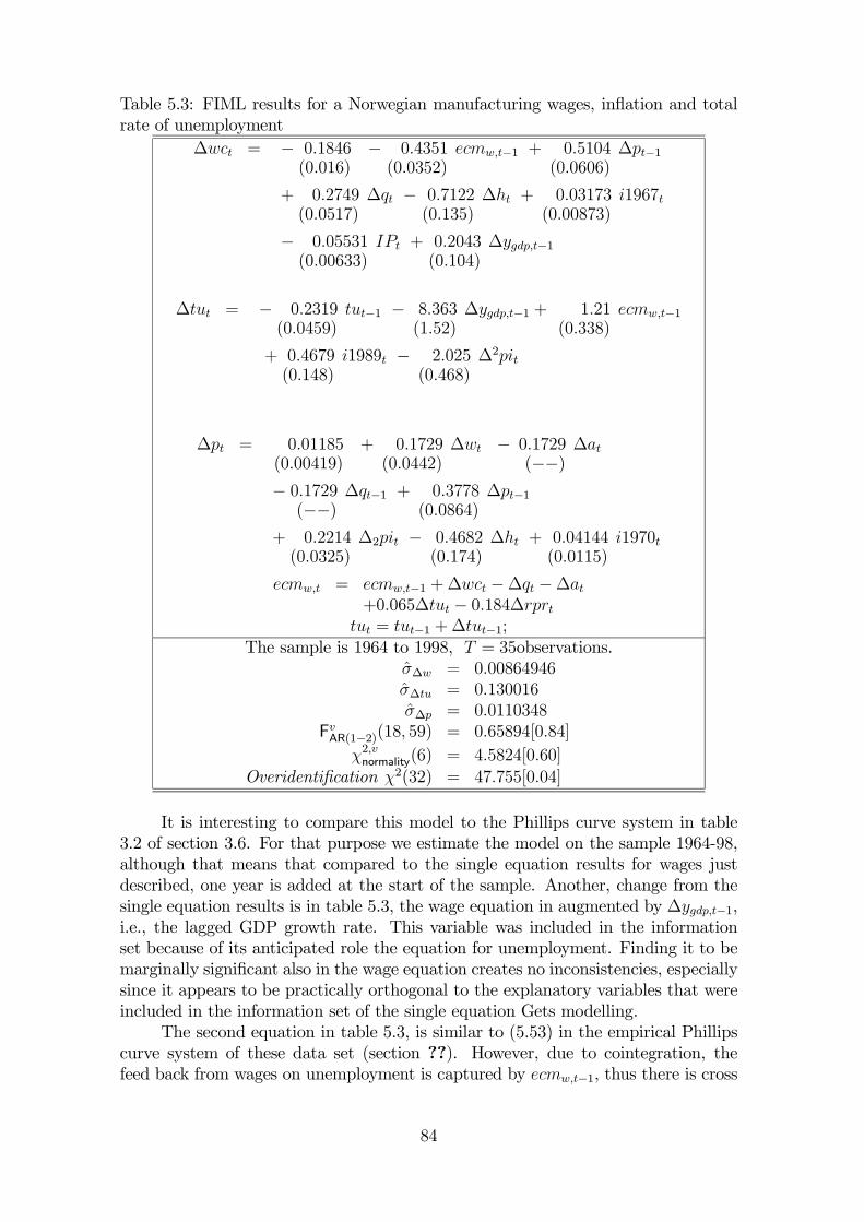
Table 5.3: FIML results for a Norwegian manufacturing wages, inflation and totalrate of unemployment
∆wct = − 0.1846(0.016)
− 0.4351(0.0352)
ecmw,t−1 + 0.5104(0.0606)
∆pt−1
+ 0.2749(0.0517)
∆qt − 0.7122(0.135)
∆ht + 0.03173(0.00873)
i1967t
− 0.05531(0.00633)
IPt + 0.2043(0.104)
∆ygdp,t−1
∆tut = − 0.2319(0.0459)
tut−1 − 8.363(1.52)
∆ygdp,t−1 + 1.21(0.338)
ecmw,t−1
+ 0.4679(0.148)
i1989t − 2.025(0.468)
∆2pit
∆pt = 0.01185(0.00419)
+ 0.1729(0.0442)
∆wt − 0.1729(−−)
∆at
− 0.1729(−−)
∆qt−1 + 0.3778(0.0864)
∆pt−1
+ 0.2214(0.0325)
∆2pit − 0.4682(0.174)
∆ht + 0.04144(0.0115)
i1970t
ecmw,t = ecmw,t−1 +∆wct −∆qt −∆at+0.065∆tut − 0.184∆rprt
tut = tut−1 +∆tut−1;The sample is 1964 to 1998, T = 35observations.
σ∆w = 0.00864946σ∆tu = 0.130016σ∆p = 0.0110348
FvAR(1−2)(18, 59) = 0.65894[0.84]
χ2,vnormality(6) = 4.5824[0.60]Overidentification χ2(32) = 47.755[0.04]
It is interesting to compare this model to the Phillips curve system in table3.2 of section 3.6. For that purpose we estimate the model on the sample 1964-98,although that means that compared to the single equation results for wages justdescribed, one year is added at the start of the sample. Another, change from thesingle equation results is in table 5.3, the wage equation in augmented by ∆ygdp,t−1,i.e., the lagged GDP growth rate. This variable was included in the informationset because of its anticipated role the equation for unemployment. Finding it to bemarginally significant also in the wage equation creates no inconsistencies, especiallysince it appears to be practically orthogonal to the explanatory variables that wereincluded in the information set of the single equation Gets modelling.
The second equation in table 5.3, is similar to (5.53) in the empirical Phillipscurve system of these data set (section ??). However, due to cointegration, thefeed back from wages on unemployment is captured by ecmw,t−1, thus there is cross
84
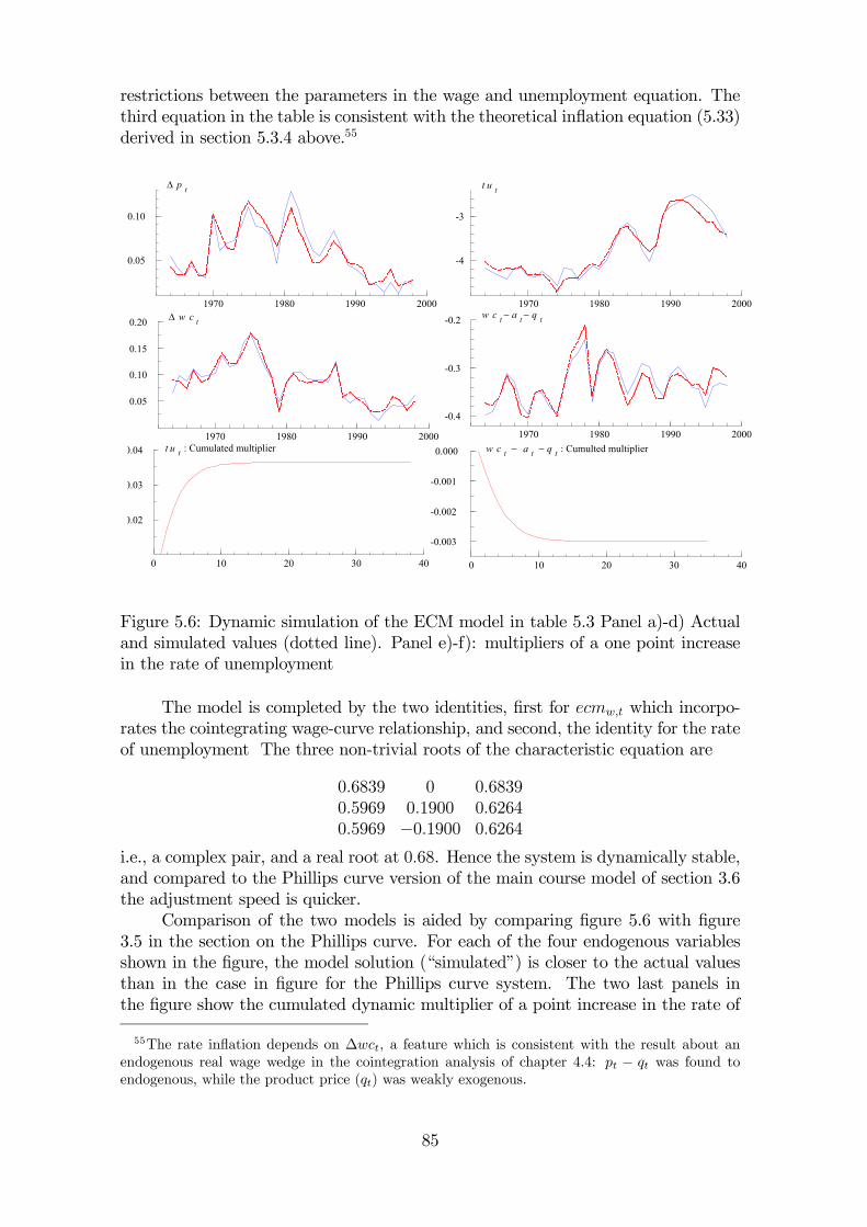
restrictions between the parameters in the wage and unemployment equation. Thethird equation in the table is consistent with the theoretical inflation equation (5.33)derived in section 5.3.4 above.55
1970 1980 1990 2000
0.05
0.10
0.15
0.20 ∆ w c t
1970 1980 1990 2000
0.05
0.10
∆ p t
1970 1980 1990 2000
-4
-3
t u t
0 10 20 30 40
0.02
0.03
0.04 t u t : Cumulated multiplier
0 10 20 30 40
-0.003
-0.002
-0.001
0.000 w c t − a t − q t : Cumulted multiplier1970 1980 1990 2000
-0.4
-0.3
-0.2 w c t − a t − q t
Figure 5.6: Dynamic simulation of the ECM model in table 5.3 Panel a)-d) Actualand simulated values (dotted line). Panel e)-f): multipliers of a one point increasein the rate of unemployment
The model is completed by the two identities, first for ecmw,t which incorpo-rates the cointegrating wage-curve relationship, and second, the identity for the rateof unemployment The three non-trivial roots of the characteristic equation are
0.6839 0 0.68390.5969 0.1900 0.62640.5969 −0.1900 0.6264
i.e., a complex pair, and a real root at 0.68. Hence the system is dynamically stable,and compared to the Phillips curve version of the main course model of section 3.6the adjustment speed is quicker.
Comparison of the two models is aided by comparing figure 5.6 with figure3.5 in the section on the Phillips curve. For each of the four endogenous variablesshown in the figure, the model solution (“simulated”) is closer to the actual valuesthan in the case in figure for the Phillips curve system. The two last panels inthe figure show the cumulated dynamic multiplier of a point increase in the rate of
55The rate inflation depends on ∆wct, a feature which is consistent with the result about anendogenous real wage wedge in the cointegration analysis of chapter 4.4: pt − qt was found toendogenous, while the product price (qt) was weakly exogenous.
85
unemployment. The difference from figure 3.5, where the steady state was not even“in sight” within the 35 years simulation period, are striking. In figure 5.6 80% ofthe long run effect is reached within 4 years, and the system is clearly stabilizing inthe course of a 10 year simulation period.
5.9 SummaryThis section has discussed extensively the modelling of the wage-price subsystem ofthe macroeconomy. We have shown that under relatively mildl assumptions aboutprice and wage setting behaviour, there exists a conditional steady state (for infla-tion, and real wages) for any given long run mean of the rate of unemployment. Theview that asymptotic stability of inflation “requires” that the rate of unemploymentsimultaneously converges to a NAIRU (which only depends on the properties ofthe wage and price and equations) has been refuted both logically and empirically.To avoid misinterpretations, it is worth restating that this result in no way jus-tify a return to demand driven macroeconomic models. Instead, as sketched in thelast section, we favour models where unemployment is determined jointly with realwages and the real exchange rate, and this implies that wage and price equations aregrafted into a bigger system of equations which also includes equations representingthe dynamics in other parts of the economy. As we have seen, the natural ratemodels in the macroeconomic literature (Phillips curve and ICM) are special casesof the model framework emerging from this section.
The finding that long run unemployment is left undetermined by the wage-price sub-model is a strong rationale for building larger systems of equations, even ifthe first objective and primary concern is the analysis of wages, prices and inflation.Another thesis of this section is that stylized wage-price models run the danger ofimposing too much in the form of nominal neutrality (absence of nominal rigidity)prior to the empirical investigation. Conversely, no inconsistencies or overdetermina-tion arise from enlarging the wage-price setting equations with a separate equationof the rate of unemployment into the system, where demand variables may enter.The enlarged model will have a steady state (given some conditions that can betested). The equilibrium rate of unemployment implied by this type of model is notof the natural rate type, since factors (in real growth rate form) from the demandside may have lasting effects. On the other hand “money illusion” is not implied,since the unemployment conditioning variables are all defined in real terms.
86
6 The New Keynesian Phillips curve
A new development of the Phillips curve framework, dubbed The New KeynesianPhillips Curve, has rapidly become a central element in modern monetary economics.This position is due to its stringent theoretical derivation, as laid out in Clarida et al.(1999) and Svensson (2000). Favourable empirical evidence is accumulating rapidly.For example, the recent studies of Galí and Gertler (1999) and Galí et al. (2001a)–hereafter GG and GGL– report empirical support for the NPC using Europeanas well as US data.
However, the methods of empirical evaluation and validating of the New Key-nesian Phillips curve found in the cited papers are informal and sometimes difficultto gauge, resting for a large part on goodnes-of-fit measures and graphs. That said,there is an emerging literature with more formal tests and evaluation methods andthis section comments this work and also suggest testing procedures not presentedelsewhere.
The New Keynesian Phillips curve, hereafter NPC, basically explains currentinflation by expected future inflation and a forcing variable, for example a measureof excess demand. Hence, compared to the other models encounter in the earliersections, the NPC is extremely stylized, since only one or two explanatory variablesof inflation are implied by theory. However, it also introduces an element whichwe have not considered systematically earlier, namely expected future inflation. Insection 6.1, we investigate the dynamic properties of the NPC, which entails notonly the NPC equation, but also specification of a process for the forcing variable.Given that a system of linear difference equations is the right framework for theo-retical discussions about stability and the type of solution (forward or backward), itfollows that the practice of deciding on these issues on the basis of single equationestimation is non-robust to extensions of the information set. For example, a for-ward solution may suggest itself from estimation of the NPC equation alone, whilesystem estimation may show that the forcing variable is endogenous, giving rise toa different set of characteristic roots and potentially giving support to a backwardsolution.
The discussion in section 6.1 covers both the pure NPC and the so called‘hybrid’ model that also includes lags of the rate of inflation, and section 6.2 discussestimation issues of the NPC, using Euro area data for illustration. In section 6.3we apply several methods for testing and evaluation of the Euro and US NPC, e.g.,goodness-of-fit and tests of significance (of forward terms and of imputed presentvalue terms). One of the messages that emerges is that emphasis on goodness-of-fitis of little value, since the fit is practically indistinguishable from modelling inflationfollowing a random walk. Building on the insight from section 6.1, we also showthat it is useful to extend the evaluation from the single equation NPC to a systemconsisting of the rate of inflation and the forcing variable.
However, as discussed in the earlier section of this book, there is a huge lit-erature (stemming back to the 1980s and 1990s) on wage and price modelling. Forexample, we have demonstrated that cointegrating relationships can be establishedbetween wages, prices, unemployment and productivity, as well as a particular or-dering of causality. In section 6.4 we show that these existing results represent newinformation relative to the NPC, and we suggest how such information can be used
87
for testing the encompassing implications of the NPC. This approach is applied toopen economy versions of the NPC, for Norway and UK.
6.1 A NPC systemThe NPC, in its pure form, states that inflation, ∆pt is explained by Et∆pt+1,expected inflation one period ahead conditonal upon information available at timet, and excess demand or marginal costs xt (e.g., output gap, the unemployment rateor the wage share in logs):
(6.1) ∆pt = βp1Et∆pt+1 + βp2xt + εpt,
where εpt is a stochastic error term. Roberts (1995) has shown that several New Key-nesian models with rational expectations have (6.1) as a common representation–including the models of staggered contracts developed by Taylor (1979, 1980)56 andCalvo (1983), and the quadratic price adjustment cost model of Rotemberg (1982).GG have given a formulation of the NPC in line with Calvo’s work: They assumethat a firm takes account of the expected future path of nominal marginal costs whensetting its price, given the likelihood that its price may remain fixed for multipleperiods. This leads to a version of the inflation equation (6.1), where the forcingvariable xt is the representative firm’s real marginal costs (measured as deviationsfrom its steady state value). They argue that the wage share (the labour incomeshare) wst is a plausible indicator for the average real marginal costs, which theyuse in the empirical analysis. The alternative, hybrid version of the NPC that usesboth Et∆pt+1 and lagged inflation as explanatory variables is also discussed below.
Equation (6.1) is incomplete as a model for inflation, since the status of xtis left unspecified. On the one hand, the use of the term forcing variable, suggestsexogeneity, whereas the custom of instrumenting the variable in estimation is ger-mane to endogeneity. In order to make progress, we therefore consider the followingcompleting system of stochastic linear difference equations57
∆pt = βp1∆pt+1 + βp2xt + εpt − bp1ηt+1(6.2)
xt = βx1∆pt−1 + βx2xt−1 + εxt(6.3)
0 ≤ |βx2| < 1The first equation is adapted from (6.1), utilizing that Et∆pt+1 = ∆pt+1 − ηt+1,where ηt+1 is the expectation error. Equation (6.3) captures that there may be feed-back from inflation on the forcing variable xt (output-gap, the rate of unemploymentor the wage share) in which case βx1 6= 0.
In order to discuss the dynamic properties of this system, re-arrange (6.2) toyield
(6.4) ∆pt+1 =1
βp1∆pt −
βp2βp1
xt − 1
βp1εpt + ηt+1
56The overlapping wage contract model of sticky prices is also attributed to Phelps (1978).57Constant terms are omitted for ease of exposition.
88
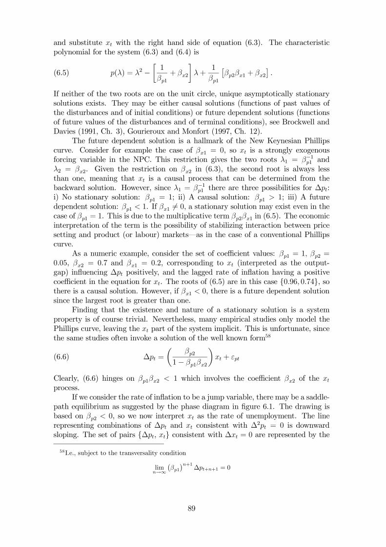
and substitute xt with the right hand side of equation (6.3). The characteristicpolynomial for the system (6.3) and (6.4) is
(6.5) p(λ) = λ2 −·1
βp1+ βx2
¸λ+
1
βp1
£βp2βx1 + βx2
¤.
If neither of the two roots are on the unit circle, unique asymptotically stationarysolutions exists. They may be either causal solutions (functions of past values ofthe disturbances and of initial conditions) or future dependent solutions (functionsof future values of the disturbances and of terminal conditions), see Brockwell andDavies (1991, Ch. 3), Gourieroux and Monfort (1997, Ch. 12).
The future dependent solution is a hallmark of the New Keynesian Phillipscurve. Consider for example the case of βx1 = 0, so xt is a strongly exogenousforcing variable in the NPC. This restriction gives the two roots λ1 = β−1p1 andλ2 = βx2. Given the restriction on βx2 in (6.3), the second root is always lessthan one, meaning that xt is a causal process that can be determined from thebackward solution. However, since λ1 = β−1p1 there are three possibilities for ∆pt:i) No stationary solution: βp1 = 1; ii) A causal solution: βp1 > 1; iii) A futuredependent solution: βp1 < 1. If βx1 6= 0, a stationary solution may exist even in thecase of βp1 = 1. This is due to the multiplicative term βp2βx1 in (6.5). The economicinterpretation of the term is the possibility of stabilizing interaction between pricesetting and product (or labour) markets–as in the case of a conventional Phillipscurve.
As a numeric example, consider the set of coefficient values: βp1 = 1, βp2 =0.05, βx2 = 0.7 and βx1 = 0.2, corresponding to xt (interpreted as the output-gap) influencing ∆pt positively, and the lagged rate of inflation having a positivecoefficient in the equation for xt. The roots of (6.5) are in this case {0.96, 0.74}, sothere is a causal solution. However, if βx1 < 0, there is a future dependent solutionsince the largest root is greater than one.
Finding that the existence and nature of a stationary solution is a systemproperty is of course trivial. Nevertheless, many empirical studies only model thePhillips curve, leaving the xt part of the system implicit. This is unfortunate, sincethe same studies often invoke a solution of the well known form58
(6.6) ∆pt =
µβp2
1− βp1βx2
¶xt + εpt
Clearly, (6.6) hinges on βp1βx2 < 1 which involves the coefficient βx2 of the xtprocess.
If we consider the rate of inflation to be a jump variable, there may be a saddle-path equilibrium as suggested by the phase diagram in figure 6.1. The drawing isbased on βp2 < 0, so we now interpret xt as the rate of unemployment. The linerepresenting combinations of ∆pt and xt consistent with ∆2pt = 0 is downwardsloping. The set of pairs {∆pt, xt} consistent with ∆xt = 0 are represented by the
58I.e., subject to the transversality condition
limn→∞
¡βp1¢n+1
∆pt+n+1 = 0
89
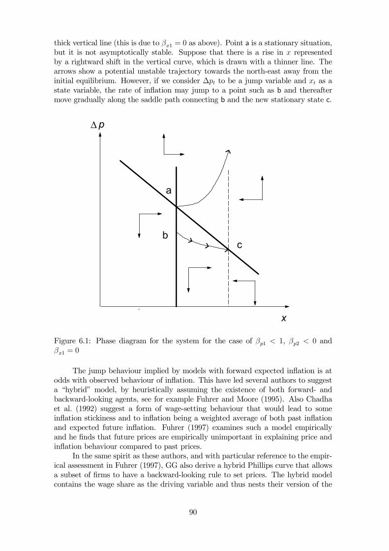
thick vertical line (this is due to βx1 = 0 as above). Point a is a stationary situation,but it is not asymptotically stable. Suppose that there is a rise in x representedby a rightward shift in the vertical curve, which is drawn with a thinner line. Thearrows show a potential unstable trajectory towards the north-east away from theinitial equilibrium. However, if we consider ∆pt to be a jump variable and xt as astate variable, the rate of inflation may jump to a point such as b and thereaftermove gradually along the saddle path connecting b and the new stationary state c.
a
bc
p∆
x
Figure 6.1: Phase diagram for the system for the case of βp1 < 1, βp2 < 0 andβx1 = 0
The jump behaviour implied by models with forward expected inflation is atodds with observed behaviour of inflation. This have led several authors to suggesta “hybrid” model, by heuristically assuming the existence of both forward- andbackward-looking agents, see for example Fuhrer and Moore (1995). Also Chadhaet al. (1992) suggest a form of wage-setting behaviour that would lead to someinflation stickiness and to inflation being a weighted average of both past inflationand expected future inflation. Fuhrer (1997) examines such a model empiricallyand he finds that future prices are empirically unimportant in explaining price andinflation behaviour compared to past prices.
In the same spirit as these authors, and with particular reference to the empir-ical assessment in Fuhrer (1997), GG also derive a hybrid Phillips curve that allowsa subset of firms to have a backward-looking rule to set prices. The hybrid modelcontains the wage share as the driving variable and thus nests their version of the
90
NPC as a special case. This amounts to the specification
(6.7) ∆pt = βfp1Et∆pt+1 + βbp1∆pt−1 + βp2xt + εpt.
GG estimate (6.7) for the U.S. in several variants –using different inflationmeasures, different normalization rules for the GMM estimation, including addi-tional lags of inflations in the equation and splitting the sample. They find thatthe overall picture remains unchanged. Marginal costs have a significant impact onshort run inflation dynamics and forward looking behavior is always found to beimportant.
In the same manner as above, equation (6.7) can be written as
(6.8) ∆pt+1 =1
βfp1∆pt −
βbp1
βfp1∆pt−1 −
βp2
βfp1xt − 1
βp1εpt + ηt+1
and combined with (6.3). The characteristic polynomial of the hybrid system is
(6.9) p(λ) = λ3 −"1
βfp1+ βx2
#λ2 +
1
βfp1
£βbp1 + βp2βx1 + βx2
¤λ− βbp1
βfp1βx2.
Using the typical results (from the studies cited below, see section 6.3.2) for theexpectation and backward-looking parameters, βfp1 = 0.25, β
bp1 = 0.75, together with
the assumption of an exogenous xt process with autoregressive parameter 0.7, weobtain the roots {3.0, 1.0, 0.7}.59 Thus, there is no asymptotically stable stationarysolution for the rate of inflation in this case.
This seems to be a common result for the hybrid model as several authorschoose to impose the restriction
(6.10) βfp1 + βbp1 = 1,
which forces a unit root upon the system. To see this, note first that a 1-1 repara-meterization of (6.8) gives
∆2pt+1 =
"1
βfp1− βbp1
βfp1− 1#∆pt +
βbp1
βfp1∆2pt −
βp2
βfp1xt − 1
βp1εpt + ηt+1,
so that if (6.10) holds, (6.8) reduces to
(6.11) ∆2pt+1 =−βp0βfp1
+(1− βfp1)
βfp1∆2pt −
βp2
βfp1xt − 1
βp1εpt + ηt+1.
Hence, the homogeneity restriction (6.10) turns the hybrid model into a model ofthe change in inflation. Equation (6.11) is an example of a model that is cast in thedifference of the original variable, a so called dVAR, only modified by the drivingvariable xt. Consequently, it represents a generalization of the random walk modelof inflation that was implied by setting βfp1 = 1 in the original NPC. The result in
59The full set of coefficients values is thus: βx1 = 0, βfp1 = 0.25, β
bp1 = 0.75, βx2 = 0.7
91
(6.11) will prove important in understanding the behaviour of the NPC in terms ofgoodness of fit, see below.
If the process xt is strongly exogenous, the NPC in (6.11) can be consideredat its own. In that case (6.11) has no stationary solution for the rate of inflation.A necessary requirement is that there are equilibrating mechanisms elsewhere inthe system, specifically in the process governing xt (e.g., the wage share). Thisrequirement parallels the case of dynamic homogeneity in the backward lookingPhillips curve ( i.e., a vertical long run Phillips curve). In the present context themessage is that statements about the stationarity of the rate of inflation, and thenature of the solution (backward or forward) requires an analysis of the system.
The empirical results of GG and GGL differ from other studies in two respects.First, βfp1 is estimated in the region (0.65, 0.85) whereas β
bp1 is one third of β
fp1 or
less. Second, GG and GGL succeed in estimating the hybrid model without imposing(6.10). GGL (their Table 2) report the estimates { 0.69, 0.27} and {0.88, 0.025} fortwo different estimation techniques. The corresponding roots are {1.09, 0.70, 0.37}and {1.11, 0.70, 0.03}, illustrating that as long as the sum of the weights is less thanone the future dependent solution prevails.
6.2 European inflation and the NPCAs mentioned above, GG and GGL use the formulation of the NPC (6.1) wherethe forcing variable xt is the wage share wst. Since under rational expectations theerrors in the forecast of ∆pt+1 and wst is uncorrelated with information dated t−1and earlier, it follows from (6.1) that
(6.12) E{(∆pt − βp1∆pt+1 − βp2wst)zt−1} = 0where zt is a vector of instruments.
The orthogonality conditions given in (6.12) form the basis for estimatingthe model with generalized method of moments (GMM). The authors report resultswhich they record as being in accordance with a priori theory. GGL report estimatesof (6.1) for the US as well as for Euroland.60 Using US data for 1960:1 to 1997:4,they report
(6.13) ∆pt = 0.924(0.029)
∆pt+1 + 0.250(0.118)
wst.
Using their aggregate data for the Euro area61 1971.3 -1998.1, we replicate theirresults for Europe:62
∆pt = 0.914(0.04)
∆pt+1 + 0.088(0.04)
wst + 0.14(0.06)
(6.14)
σ = 0.321 χ2J (9) = 8.21 [0.51]
60These estimates are - somewhat confusingly - called “reduced form” estimates in GG andGGL, meaning that the ”deep” structural parameters of their model are not identified and hencenot estimated in this linear relationsship between ∆pt, Et{∆pt+1} and wst.
61See the Appendix B and Fagan et al. (2001).62That is, equation (13) in GGL. We are grateful to J. David López-Salido of the Bank of Spain,
who kindly provided us with the data for the Euro area and a RATS-program used in GGL.
92
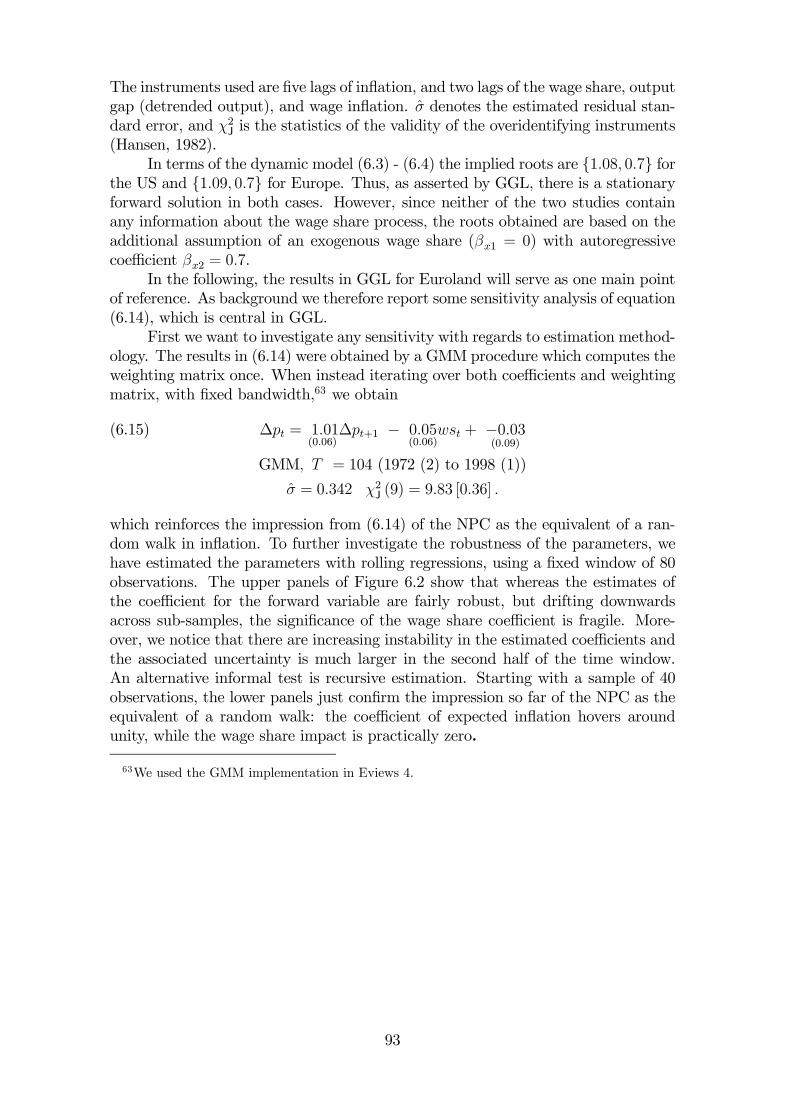
The instruments used are five lags of inflation, and two lags of the wage share, outputgap (detrended output), and wage inflation. σ denotes the estimated residual stan-dard error, and χ2J is the statistics of the validity of the overidentifying instruments(Hansen, 1982).
In terms of the dynamic model (6.3) - (6.4) the implied roots are {1.08, 0.7} forthe US and {1.09, 0.7} for Europe. Thus, as asserted by GGL, there is a stationaryforward solution in both cases. However, since neither of the two studies containany information about the wage share process, the roots obtained are based on theadditional assumption of an exogenous wage share (βx1 = 0) with autoregressivecoefficient βx2 = 0.7.
In the following, the results in GGL for Euroland will serve as one main pointof reference. As background we therefore report some sensitivity analysis of equation(6.14), which is central in GGL.
First we want to investigate any sensitivity with regards to estimation method-ology. The results in (6.14) were obtained by a GMM procedure which computes theweighting matrix once. When instead iterating over both coefficients and weightingmatrix, with fixed bandwidth,63 we obtain
∆pt = 1.01(0.06)
∆pt+1 − 0.05(0.06)
wst + −0.03(0.09)
(6.15)
GMM, T = 104 (1972 (2) to 1998 (1))
σ = 0.342 χ2J (9) = 9.83 [0.36] .
which reinforces the impression from (6.14) of the NPC as the equivalent of a ran-dom walk in inflation. To further investigate the robustness of the parameters, wehave estimated the parameters with rolling regressions, using a fixed window of 80observations. The upper panels of Figure 6.2 show that whereas the estimates ofthe coefficient for the forward variable are fairly robust, but drifting downwardsacross sub-samples, the significance of the wage share coefficient is fragile. More-over, we notice that there are increasing instability in the estimated coefficients andthe associated uncertainty is much larger in the second half of the time window.An alternative informal test is recursive estimation. Starting with a sample of 40observations, the lower panels just confirm the impression so far of the NPC as theequivalent of a random walk: the coefficient of expected inflation hovers aroundunity, while the wage share impact is practically zero.
63We used the GMM implementation in Eviews 4.
93
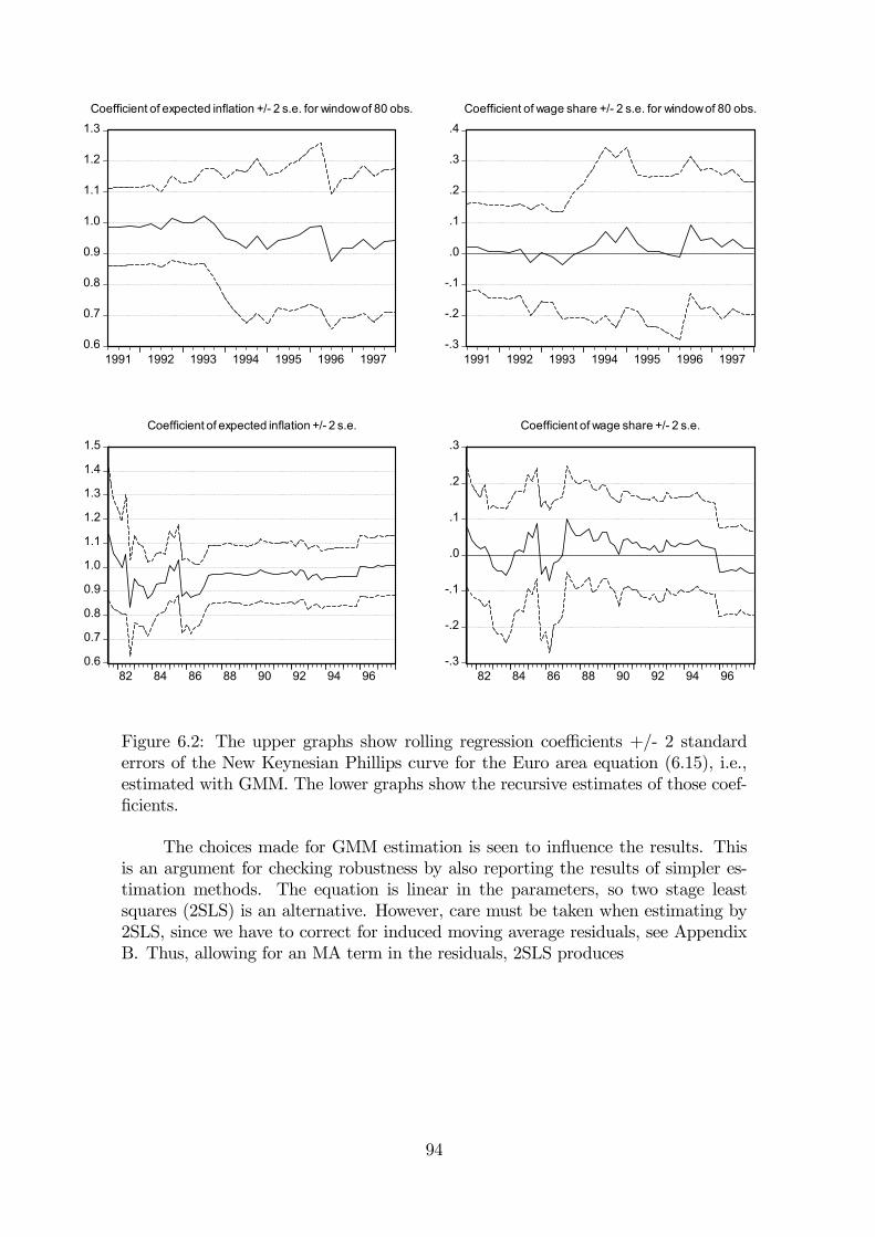
0.6
0.7
0.8
0.9
1.0
1.1
1.2
1.3
1991 1992 1993 1994 1995 1996 1997
Coefficient of expected inflation +/- 2 s.e. for window of 80 obs.
-.3
-.2
-.1
.0
.1
.2
.3
.4
1991 1992 1993 1994 1995 1996 1997
Coefficient of wage share +/- 2 s.e. for window of 80 obs.
0.6
0.7
0.8
0.9
1.0
1.1
1.2
1.3
1.4
1.5
82 84 86 88 90 92 94 96
Coefficient of expected inflation +/- 2 s.e.
-.3
-.2
-.1
.0
.1
.2
.3
82 84 86 88 90 92 94 96
Coefficient of wage share +/- 2 s.e.
Figure 6.2: The upper graphs show rolling regression coefficients +/- 2 standarderrors of the New Keynesian Phillips curve for the Euro area equation (6.15), i.e.,estimated with GMM. The lower graphs show the recursive estimates of those coef-ficients.
The choices made for GMM estimation is seen to influence the results. Thisis an argument for checking robustness by also reporting the results of simpler es-timation methods. The equation is linear in the parameters, so two stage leastsquares (2SLS) is an alternative. However, care must be taken when estimating by2SLS, since we have to correct for induced moving average residuals, see AppendixB. Thus, allowing for an MA term in the residuals, 2SLS produces
94
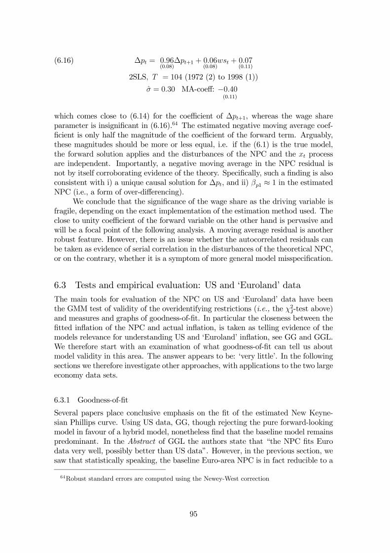
∆pt = 0.96(0.08)
∆pt+1 + 0.06(0.08)
wst + 0.07(0.11)
(6.16)
2SLS, T = 104 (1972 (2) to 1998 (1))
σ = 0.30 MA-coeff: −0.40(0.11)
which comes close to (6.14) for the coefficient of ∆pt+1, whereas the wage shareparameter is insignificant in (6.16).64 The estimated negative moving average coef-ficient is only half the magnitude of the coefficient of the forward term. Arguably,these magnitudes should be more or less equal, i.e. if the (6.1) is the true model,the forward solution applies and the disturbances of the NPC and the xt processare independent. Importantly, a negative moving average in the NPC residual isnot by itself corroborating evidence of the theory. Specifically, such a finding is alsoconsistent with i) a unique causal solution for ∆pt, and ii) βp1 ≈ 1 in the estimatedNPC (i.e., a form of over-differencing).
We conclude that the significance of the wage share as the driving variable isfragile, depending on the exact implementation of the estimation method used. Theclose to unity coefficient of the forward variable on the other hand is pervasive andwill be a focal point of the following analysis. A moving average residual is anotherrobust feature. However, there is an issue whether the autocorrelated residuals canbe taken as evidence of serial correlation in the disturbances of the theoretical NPC,or on the contrary, whether it is a symptom of more general model misspecification.
6.3 Tests and empirical evaluation: US and ‘Euroland’ dataThe main tools for evaluation of the NPC on US and ‘Euroland’ data have beenthe GMM test of validity of the overidentifying restrictions (i.e., the χ2J-test above)and measures and graphs of goodness-of-fit. In particular the closeness between thefitted inflation of the NPC and actual inflation, is taken as telling evidence of themodels relevance for understanding US and ‘Euroland’ inflation, see GG and GGL.We therefore start with an examination of what goodness-of-fit can tell us aboutmodel validity in this area. The answer appears to be: ‘very little’. In the followingsections we therefore investigate other approaches, with applications to the two largeeconomy data sets.
6.3.1 Goodness-of-fit
Several papers place conclusive emphasis on the fit of the estimated New Keyne-sian Phillips curve. Using US data, GG, though rejecting the pure forward-lookingmodel in favour of a hybrid model, nonetheless find that the baseline model remainspredominant. In the Abstract of GGL the authors state that “the NPC fits Eurodata very well, possibly better than US data”. However, in the previous section, wesaw that statistically speaking, the baseline Euro-area NPC is in fact reducible to a
64Robust standard errors are computed using the Newey-West correction
95
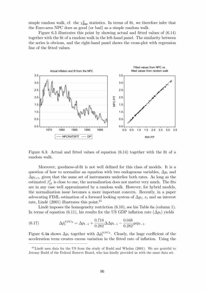
simple random walk, cf. the χ2RW statistics. In terms of fit, we therefore infer thatthe Euro-area NPC does as good (or bad) as a simple random walk.
Figure 6.3 illustrates this point by showing actual and fitted values of (6.14)together with the fit of a random walk in the left-hand panel. The similarity betweenthe series is obvious, and the right-hand panel shows the cross-plot with regressionline of the fitted values.
0.0
0.5
1.0
1.5
2.0
2.5
3.0
3.5
1975 1980 1985 1990 1995
NPCRATSFIT DP
0.0
0.5
1.0
1.5
2.0
2.5
3.0
3.5
0.0 0.5 1.0 1.5 2.0 2.5 3.0 3.5
RW-FIT
NPC
-FIT
Fitted values from NPC vs.fitted values from random walkActual inflation and fit from the NPC
Figure 6.3: Actual and fitted values of equation (6.14) together with the fit of arandom walk.
Moreover, goodness-of-fit is not well defined for this class of models. It is aquestion of how to normalize an equation with two endogenous variables, ∆pt and∆pt+1, given that the same set of instruments underlies both rates. As long as theestimated βfp1 is close to one, the normalization does not matter very much. The fitsare in any case well approximated by a random walk. However, for hybrid models,the normalization issue becomes a more important concern. Recently, in a paperadvocating FIML estimation of a forward looking system of ∆pt, xt and an interestrate, Lindé (2001) illustrates this point.65
Lindé imposes the homogeneity restriction (6.10), see his Table 6a (column 1).In terms of equation (6.11), his results for the US GDP inflation rate (∆pt) yields
(6.17) ∆pNPCat = ∆pt−1 +
0.718
0.282∆∆pt−1 − 0.048
0.282gapt−1.
Figure 6.4a shows ∆pt together with ∆pNPCat . Clearly, the huge coefficient of the
acceleration term creates excess variation in the fitted rate of inflation. Using the
65Lindé uses data for the US from the study of Rudd and Whelan (2001). We are grateful toJeromy Rudd of the Federal Reserve Board, who has kindly provided us with the same data set.
96
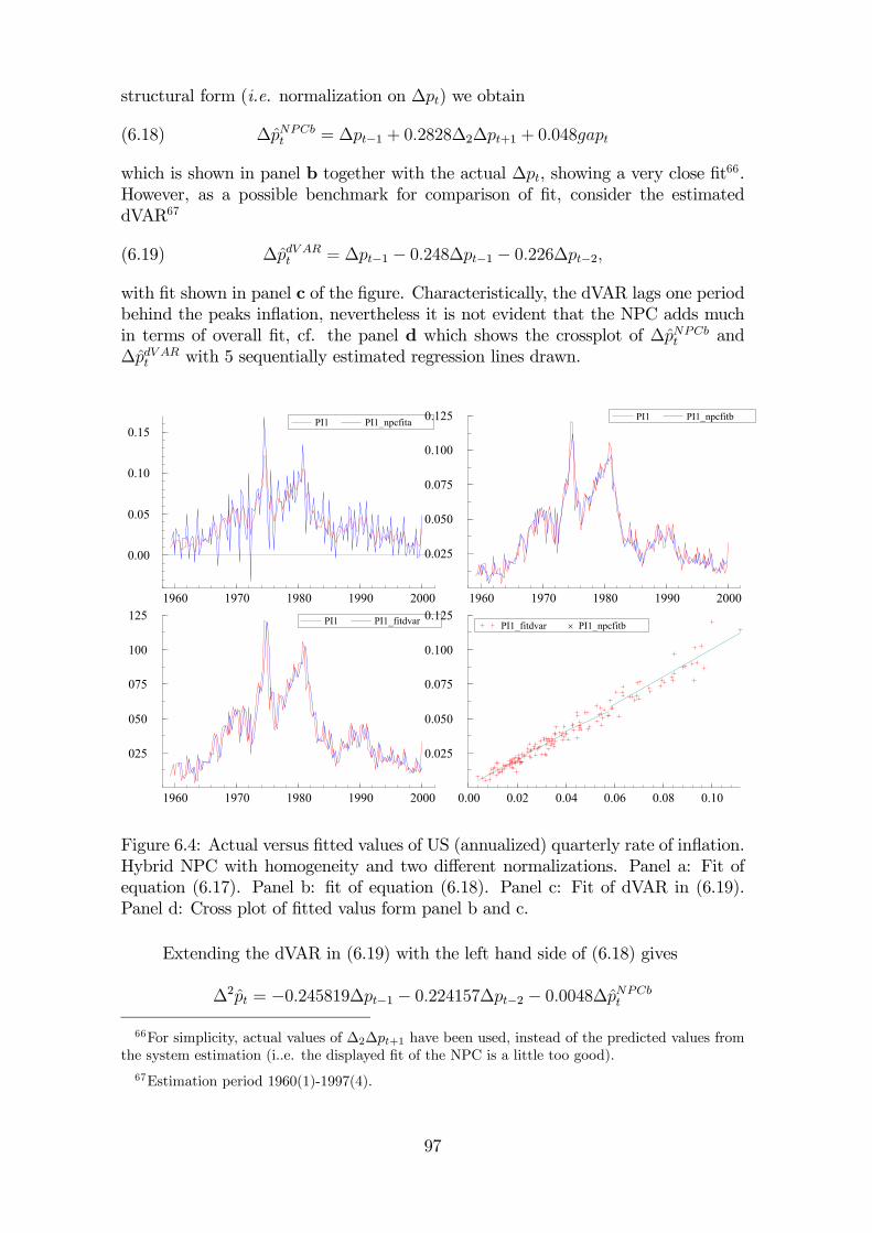
structural form (i.e. normalization on ∆pt) we obtain
(6.18) ∆pNPCbt = ∆pt−1 + 0.2828∆2∆pt+1 + 0.048gapt
which is shown in panel b together with the actual ∆pt, showing a very close fit66.However, as a possible benchmark for comparison of fit, consider the estimateddVAR67
(6.19) ∆pdV ARt = ∆pt−1 − 0.248∆pt−1 − 0.226∆pt−2,
with fit shown in panel c of the figure. Characteristically, the dVAR lags one periodbehind the peaks inflation, nevertheless it is not evident that the NPC adds muchin terms of overall fit, cf. the panel d which shows the crossplot of ∆pNPCb
t and∆pdV ARt with 5 sequentially estimated regression lines drawn.
1960 1970 1980 1990 2000
0.00
0.05
0.10
0.15PI1 PI1_npcfita
1960 1970 1980 1990 2000
0.025
0.050
0.075
0.100
0.125 PI1 PI1_npcfitb
1960 1970 1980 1990 2000
025
050
075
100
125 PI1 PI1_fitdvar
0.00 0.02 0.04 0.06 0.08 0.10
0.025
0.050
0.075
0.100
0.125PI1_fitdvar × PI1_npcfitb
Figure 6.4: Actual versus fitted values of US (annualized) quarterly rate of inflation.Hybrid NPC with homogeneity and two different normalizations. Panel a: Fit ofequation (6.17). Panel b: fit of equation (6.18). Panel c: Fit of dVAR in (6.19).Panel d: Cross plot of fitted valus form panel b and c.
Extending the dVAR in (6.19) with the left hand side of (6.18) gives
∆2pt = −0.245819∆pt−1 − 0.224157∆pt−2 − 0.0048∆pNPCbt
66For simplicity, actual values of ∆2∆pt+1 have been used, instead of the predicted values fromthe system estimation (i..e. the displayed fit of the NPC is a little too good).67Estimation period 1960(1)-1997(4).
97
showing that the fitted values from the structural NPC add nothing to the fit of thedVAR.
It seems reasonable to conclude that by themselves, graphs showing the goodness-of-fit tell very little about how well the estimated NPCs approximate reality. At thevery least, the NPC fit should be compared to the fit of a simple random walk orof a more general equation in differences (a dVAR). It is interesting to note that, inthe cases we have analyzed, the fit of the random walk/dVAR is as good as or betterthan the NPC-fit. The goodness-of-fit is not invariant to the chosen normalization,unless the forward term is close to unity, and this creates an ‘indeterminateness’about the goodness-of-fit also as a descriptive device.
There is thus a need for other evaluation methods, and in the rest of thissection we consider significance testing of the forward term, and of the use of theclosed form solution for testing purposes. In section 6.4 we turn to the testing of theencompassing implications of the NPC for existing econometric models of inflation.
6.3.2 Tests of significance of the forward term
For the original NPC in equation (6.1) one would certainly expect to estimate a βp1that leads to rejection of the null hypothesis that βp1 = 0. This is simply becausethere is typically a lot of autocorrelation in the rate of inflation, beyond what canbe explained by the xt variable or its lag. Thus, at the outset it seems more sensibleto base significance testing of the forward term in the hybrid model.
The empirical evidence based on US data is not unanimous: GG and GGL findthat the coefficient of the forward variable outweigh the backward coefficient by 3to 1 or more, whereas Fuhrer (1997) reports the opposite relative weights. Fuhrer’sfindings are reinforced by Rudd and Whelan (2001), see below, and by Lindé (2001)who reports the weights 0.75 for the backward variable and 0.25 for the forwardvariable, while finding the latter significantly different from zero.
However, Rudd and Whelan (2001) in their appraisal of GG, show that caremust be taken when interpreting the significance of the forward term in the hybridmodel. In particular, they show that the high estimates of βfp1 and low estimates ofβbp1 may be expected if the true model is in fact of a conventional (causal) type:
∆pt = βp0 + βp3∆pt−1 + βp4zt + pt
where zt is a relevant explanatory variable that is not perfectly correlated with thedriving variable of the NPC (i.e., xt) and pt is an innovation process.
This occurs when a variable zt that belongs to the true model is left outof the specification under study. The disturbance (6.7) is then no longer a pureexpectations error, because it includes the influence of zt on inflation. Rudd andWhelan show that the estimates of βfp1 will be biased upwards as long as ∆pt+1and the variables used to instrument it are both correlated with zt. Moreover, theydemonstrate that the bias is likely to be large. Nevertheless, they are pessimisticabout the possibility of detecting the bias with Hansen’s χ2J statistic due to lowpower. That said, the basic logic of Rudd and Whelan’s analysis about biasedcoefficients of forward variables remains valid, and its empirical relevance should bechecked on the specific data sets used in the literature.
98
Equation (6.20) and (6.21) present the results for the Euro area hybrid model,first using GMM and then 2SLS with a moving average disturbance term:
∆pt = 0.65(0.07)
∆pt+1 + 0.34(007)
∆pt−1 + 0.03(0.05)
wst
+ 0.04(0.1182)
(6.20)
GMM, T = 104 (1972 (2) to 1998 (1))
σ = 0.277 χ2J (6) = 7.55 [0.27]
∆pt = 0.62(0.09)
∆pt+1 + 0.39(0.07)
∆pt−1 − 0.008(0.03)
wst
− 0.01(0.04)
(6.21)
2SLS, T = 104 (1972 (2) to 1998 (1))
σ = 0.19 MA-coeff: −0.75(0.18)
The same instruments as GGL are used, with some minor changes68: First, we usean alternative output-gap measure (emugapt), which is a simple transformation ofthe one defined in Fagan et al. (2001) as (the log of) real output relative to potentialoutput, measured by a constant-return-to-scale Cobb-Douglas production functionwith neutral technical progress, see Appendix B. We have also omitted two lagsof the growth rate of wage inflation in order to limit the number of equations inthe system version of the NPC that we estimate in section 6.3.5. Despite thesemodifications, the coefficient estimates of the inflation terms are in good accordancewith GGL, and also with the results reported by GG on US data.
In the same way as for the pure NPC, there is clear indication of a unit root (thetwo inflation coefficients sum to one), and the wage share again plays an unimportantrole in the specification. On the other hand, the formal significance of the forwardterm, and the insignificance of the J-statistic by themselves corroborate the NPC asa relevant model for European inflation dynamics.
However, the overriding question is whether (6.20) and/or (6.21), when viewedas statistical models, give rise to valid inference about the significance of the for-ward coefficient. In other words, the statistical adequacy of the models for testingpurposes is a concern. In this perspective, the practice of ‘whitening’ the resid-uals (GMM or MA(1) correction in 2SLS), is problematic, since one then tacitlyassume that serial correlation in the residuals is symptomatic of serial correlationin the true disturbances. Thus, the specification of the econometric model used fortesting a substantive hypothesis (the role of the forward variable), incorporates thealternative hypothesis associated with a misspecification test (i.e., of residual auto-correlation). This is usually not a good idea in econometrics, since the underlyingcause of the residual misspecification may be quite different, for example omittedvariables, wrong functional form or, in this case, a certain form of over-differencing.
68See below equation (6.14) in section 6.2.
99
Instead, when departures from the underlying assumptions of the statistical modelhave been established, there is need for respecification, with the aim of finding astatistical model which does a better job in capturing the systematic variation inthe rate of inflation, see e.g., Harvey (1981, Ch. 8.4), Hendry (1983) and Spanos(1986, Ch. 26) for general discussions.69.
As an example of this approach, consider first the hybrid NPC estimated by2SLS without MA(1) correction:
∆pt = 0.6551(0.135)
∆pt+1 + 0.28(0.117)
∆pt−1 + 0.071(0.086)
wst
+ 0.1027(0.1182)
(6.22)
2SLS, T = 104 (1972 (2) to 1998 (1))
σIV = 0.276711 RSS = 7.65689519FAR(1−1) = 166.93[0.0000] FAR(2−2) = 4.7294[0.0320]FARCH(1−4) = 2.4713[0.050] χ2normality = 1.5924[0.4510]FHETx2 = 2.6807[0.0191] FHETxixj = 2.3445[0.0200]
The misspecification tests in (6.22) show that the (uncorrected) hybrid model resid-uals are characterized not only by first order autocorrelation (which may be inducedby the errors in variables estimation method), but also by second order autocorrela-tion and by heteroscedasticity70. Thus, the equation appears to be inadequate as astatistical model of the rate of inflation, and does not provide the basis for reliableinference about parameters of interest (e.g., the coefficient of the forward term andthe characteristic roots). As pointed out, the popular route around this is eitherto ‘whiten’ the residuals (GMM), and/or to correct the 2SLS coefficient standarderrors. However, another way of whitening the residuals is to respecify the model,with the aim of attaining innovation error processes and a firmer basis for testinghypothesis within the respecified model.
In the present case, likely directions for respecification are suggested by pre-existing results from several decades of empirical modelling of inflation dynamics.For example, variables representing capacity utilization (output-gap and/or unem-ployment) have a natural role in inflation models. Additional lags in the rate ofinflation are also obvious candidates. As a direct test of this respecification, wemoved the lagged output-gap (emugapt−1) and the fourth lag of inflation (∆pt−4)from the list of instruments used for estimation of (6.21), and included them as ex-
69There is a clear parallel to the fallacy of choosing a common factor model (RALS estimation)on the basis of finding that the residuals of a static model are autocorrelated, Hendry and Mizon(1978), Hendry (1995a, Ch. 7.7) and Mizon (1995).70The reported statistics: F distributed tests of autoregressive residual autocorrelation
(FAR(1−1)and FAR(2−2)), see Godfrey (1978) and Doornik (1996); autoregressive conditional het-eroscedasticity (FARCH(1−4)), see Engle (1982); and heteroscedasticity due to cross products ofthe regressors (FHETxixj ), see White (1980) and Doornik (1996), whereas FHETx2 is a test of het-eroscedasticity due to squares of the regressors. The Chi-square test of residual non-normality(χ2normality) is from Doornik and Hansen (1994).
100
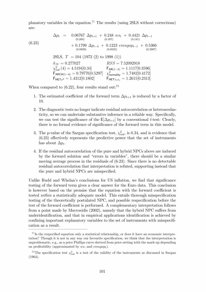
planatory variables in the equation.71 The results (using 2SLS without corrections)are:
∆pt = 0.06767(0.284)
∆pt+1 + 0.248(0.167)
wst + 0.4421(0.141)
∆pt−1
+ 0.1799(0.0939)
∆pt−4 + 0.1223(0.0525)
emugapt−1 + 0.5366(0.2997)
(6.23)
2SLS, T = 104 (1972 (2) to 1998 (1))
σIV = 0.277027 RSS = 7.52092918χ2ival (4) = 4.5194[0.34] FAR(1−5) = 1.1117[0.3596]FARCH(1−4) = 0.79776[0.5297] χ2normality = 1.7482[0.4172]FHETx2 = 1.4312[0.1802] FHETxixj = 1.2615[0.2313]
When compared to (6.22), four results stand out:72
1. The estimated coefficient of the forward term ∆pt+1 is reduced by a factor of10.
2. The diagnostic tests no longer indicate residual autocorrelation or heteroscedas-ticity, so we can undertake substantive inference in a reliable way. Specifically,we can test the significance of the E[∆pt+1] by a conventional t-test: Clearly,there is no formal evidence of significance of the forward term in this model.
3. The p-value of the Sargan specification test, χ2ival, is 0.34, and is evidence that(6.23) effectively represents the predictive power that the set of instrumentshas about ∆pt.
4. If the residual autocorrelation of the pure and hybrid NPCs above are inducedby the forward solution and “errors in variables”, there should be a similarmoving average process in the residuals of (6.23). Since there is no detectableresidual autocorrelation that interpretation is refuted, supporting instead thatthe pure and hybrid NPCs are misspecified.
Unlike Rudd and Whelan’s conclusions for US inflation, we find that significancetesting of the forward term gives a clear answer for the Euro data. This conclusionis however based on the premise that the equation with the forward coefficient istested within a statistically adequate model. This entails thorough misspecificationtesting of the theoretically postulated NPC, and possible respecification before thetest of the forward coefficient is performed. A complementary interpretation followsfrom a point made by Mavroeidis (2002), namely that the hybrid NPC suffers fromunderidentification, and that in empirical applications identification is achieved byconfining important explanatory variables to the set of instruments with misspecifi-cation as a result.
71Is the respecified equation only a statistical relationship, or does it have an economic interpre-tation? Though it is not in any way our favourite specification, we think that the interpretation isunproblematic, e.g., as a price Phillips curve derived from price setting with the mark-up dependingon profitability (approximated by ws, and emugapt).72The specification test χ2ival is a test of the validity of the instruments as discussed in Sargan
(1964).
101
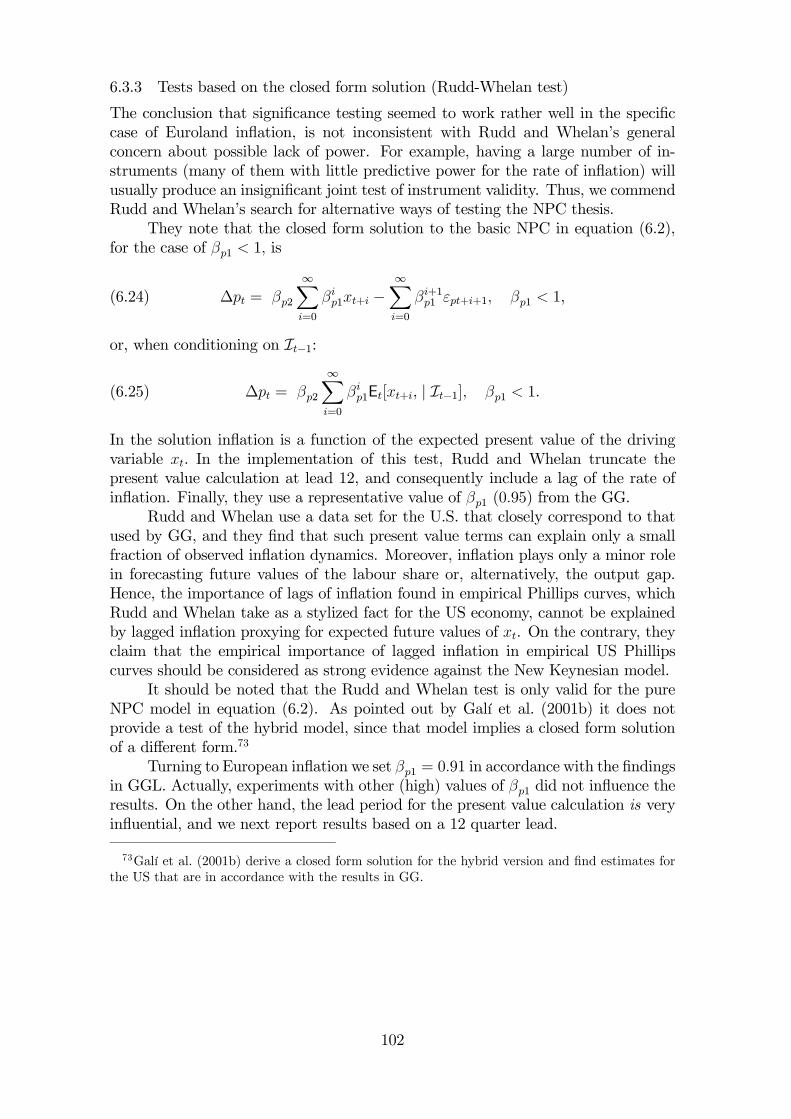
6.3.3 Tests based on the closed form solution (Rudd-Whelan test)
The conclusion that significance testing seemed to work rather well in the specificcase of Euroland inflation, is not inconsistent with Rudd and Whelan’s generalconcern about possible lack of power. For example, having a large number of in-struments (many of them with little predictive power for the rate of inflation) willusually produce an insignificant joint test of instrument validity. Thus, we commendRudd and Whelan’s search for alternative ways of testing the NPC thesis.
They note that the closed form solution to the basic NPC in equation (6.2),for the case of βp1 < 1, is
(6.24) ∆pt = βp2
∞Xi=0
βip1xt+i −∞Xi=0
βi+1p1 εpt+i+1, βp1 < 1,
or, when conditioning on It−1:
(6.25) ∆pt = βp2
∞Xi=0
βip1Et[xt+i, | It−1], βp1 < 1.
In the solution inflation is a function of the expected present value of the drivingvariable xt. In the implementation of this test, Rudd and Whelan truncate thepresent value calculation at lead 12, and consequently include a lag of the rate ofinflation. Finally, they use a representative value of βp1 (0.95) from the GG.
Rudd and Whelan use a data set for the U.S. that closely correspond to thatused by GG, and they find that such present value terms can explain only a smallfraction of observed inflation dynamics. Moreover, inflation plays only a minor rolein forecasting future values of the labour share or, alternatively, the output gap.Hence, the importance of lags of inflation found in empirical Phillips curves, whichRudd and Whelan take as a stylized fact for the US economy, cannot be explainedby lagged inflation proxying for expected future values of xt. On the contrary, theyclaim that the empirical importance of lagged inflation in empirical US Phillipscurves should be considered as strong evidence against the New Keynesian model.
It should be noted that the Rudd and Whelan test is only valid for the pureNPC model in equation (6.2). As pointed out by Galí et al. (2001b) it does notprovide a test of the hybrid model, since that model implies a closed form solutionof a different form.73
Turning to European inflation we set βp1 = 0.91 in accordance with the findingsin GGL. Actually, experiments with other (high) values of βp1 did not influence theresults. On the other hand, the lead period for the present value calculation is veryinfluential, and we next report results based on a 12 quarter lead.
73Galí et al. (2001b) derive a closed form solution for the hybrid version and find estimates forthe US that are in accordance with the results in GG.
102
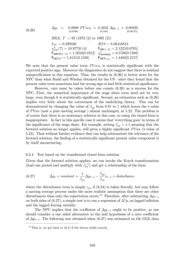
∆pt = 0.0989(0.0198)
PV wst + 0.4033(0.108)
∆pt−1 + 0.00939(0.00175)(6.26)
2SLS, T = 93 (1972 (2) to 1995 (2))
σIV = 0.299336 RSS = 8.06416813χ2ival (7) = 10.977[0.14] FAR(1−5) = 2.1225[0.0705]FARCH(1−4) = 1.5658[0.1912] χ2normality = 0.5786[0.7488]FHETx2 = 1.8131[0.1338] FHETxixj = 1.4480[0.2157]
We note that the present value term PV wst is statistically significant with theexpected positive sign. Moreover the diagnostics do not suggest that there is residualmisspecification in this equation. Thus, the results in (6.26) is better news for theNPC than what Rudd and Whelan obtained for the US–since they found that thepresent value term sometimes had the wrong sign or had little statistical significance.
However, care must be taken before one counts (6.26) as a success for theNPC. First, the numerical importance of the wage share term need not be verylarge, even though it is statistically significant. Second, an estimation such as (6.26)implies very little about the correctness of the underlying theory. This can bedemonstrated by changing the value of βp1 from 0.91 to 1 which leaves the t-valueof PVws (now a pure moving average ) almost unchanged, at 5.22. The problem isof course that there is no stationary solution in this case, so using the closed form isinappropriate. In fact in this specific case it seems that ‘everything goes’ in terms ofthe significance of the wage share. For example, setting βp1 = 1.1 meaning that theforward solution no longer applies, still gives a highly significant PVws, (t-value of5.23). Thus without further evidence that can help substantiate the relevance of theforward solution, the finding of a statistically significant present value component isby itself unconvincing.
6.3.4 Test based on the transformed closed form solution
Given that the forward solution applies, we can invoke the Koyck transformation(lead one period and multiply with β−1p1 ) and get a relationship of the form
(6.27) ∆pt = constant +1
βp1∆pt−1 −
βp2βp1
xt−1 + disturbance.
where the disturbance term is simply εp,t if (6.24) is taken literally, but may followa moving average process under the more realistic assumption that there are otherdisturbances than only the expectation errors.74 Therefore, after subtracting ∆pt−1on both sides of (6.27), a simple test is to run a regression of ∆2pt on lagged inflationand the lagged forcing variable.
The NPC implies that the coefficient of ∆pt−1 ought to be positive, so oneshould consider a one sided alternative to the null hypothesis of a zero coefficientof ∆pt−1. The following was obtained when (6.27) was estimated on the GGL data
74That is, we get back to (6.4) if the theory holds exactly.
103
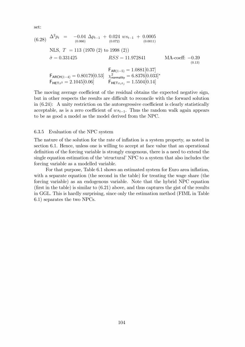
set:
∆2pt = −0.04(0.066)
∆pt−1 + 0.024(0.072)
wst−1 + 0.0005(0.0011)(6.28)
NLS, T = 113 (1970 (2) to 1998 (2))
σ = 0.331425 RSS = 11.972841 MA-coeff: −0.39(0.13)
FAR(1−5) = 1.0881[0.37]FARCH(1−4) = 0.80179[0.53] χ2normality = 6.8376[0.033]
∗
FHETx2 = 2.1045[0.06] FHETxixj = 1.5504[0.14]
The moving average coefficient of the residual obtains the expected negative sign,but in other respects the results are difficult to reconcile with the forward solutionin (6.24): A unity restriction on the autoregressive coefficient is clearly statisticallyacceptable, as is a zero coefficient of wst−1. Thus the random walk again appearsto be as good a model as the model derived from the NPC.
6.3.5 Evaluation of the NPC system
The nature of the solution for the rate of inflation is a system property, as noted insection 6.1. Hence, unless one is willing to accept at face value that an operationaldefinition of the forcing variable is strongly exogenous, there is a need to extend thesingle equation estimation of the ‘structural’ NPC to a system that also includes theforcing variable as a modelled variable.
For that purpose, Table 6.1 shows an estimated system for Euro area inflation,with a separate equation (the second in the table) for treating the wage share (theforcing variable) as an endogenous variable. Note that the hybrid NPC equation(first in the table) is similar to (6.21) above, and thus captures the gist of the resultsin GGL. This is hardly surprising, since only the estimation method (FIML in Table6.1) separates the two NPCs.
104
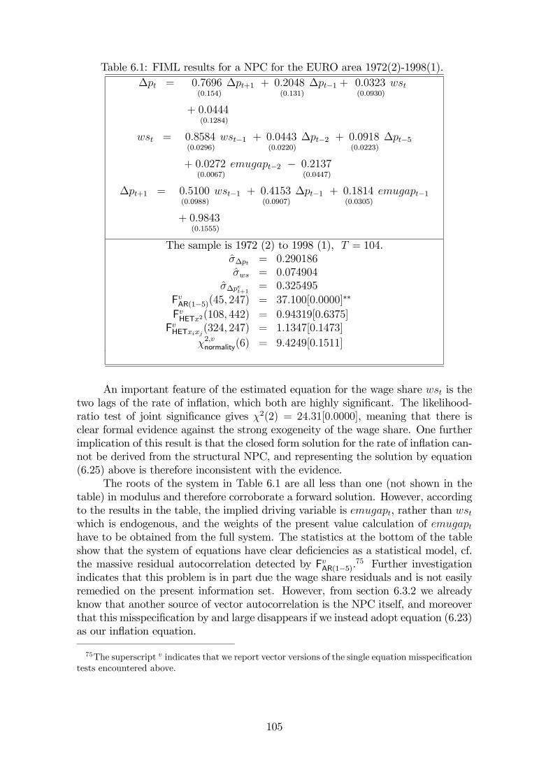
Table 6.1: FIML results for a NPC for the EURO area 1972(2)-1998(1).∆pt = 0.7696
(0.154)
∆pt+1 + 0.2048(0.131)
∆pt−1 + 0.0323(0.0930)
wst
+ 0.0444(0.1284)
wst = 0.8584(0.0296)
wst−1 + 0.0443(0.0220)
∆pt−2 + 0.0918(0.0223)
∆pt−5
+ 0.0272(0.0067)
emugapt−2 − 0.2137(0.0447)
∆pt+1 = 0.5100(0.0988)
wst−1 + 0.4153(0.0907)
∆pt−1 + 0.1814(0.0305)
emugapt−1
+ 0.9843(0.1555)
The sample is 1972 (2) to 1998 (1), T = 104.σ∆pt = 0.290186σws = 0.074904
σ∆pet+1= 0.325495
FvAR(1−5)(45, 247) = 37.100[0.0000]∗∗
FvHETx2(108, 442) = 0.94319[0.6375]FvHETxixj(324, 247) = 1.1347[0.1473]
χ2,vnormality(6) = 9.4249[0.1511]
An important feature of the estimated equation for the wage share wst is thetwo lags of the rate of inflation, which both are highly significant. The likelihood-ratio test of joint significance gives χ2(2) = 24.31[0.0000], meaning that there isclear formal evidence against the strong exogeneity of the wage share. One furtherimplication of this result is that the closed form solution for the rate of inflation can-not be derived from the structural NPC, and representing the solution by equation(6.25) above is therefore inconsistent with the evidence.
The roots of the system in Table 6.1 are all less than one (not shown in thetable) in modulus and therefore corroborate a forward solution. However, accordingto the results in the table, the implied driving variable is emugapt, rather than wstwhich is endogenous, and the weights of the present value calculation of emugapthave to be obtained from the full system. The statistics at the bottom of the tableshow that the system of equations have clear deficiencies as a statistical model, cf.the massive residual autocorrelation detected by FvAR(1−5).
75 Further investigationindicates that this problem is in part due the wage share residuals and is not easilyremedied on the present information set. However, from section 6.3.2 we alreadyknow that another source of vector autocorrelation is the NPC itself, and moreoverthat this misspecification by and large disappears if we instead adopt equation (6.23)as our inflation equation.
75The superscript v indicates that we report vector versions of the single equation misspecificationtests encountered above.
105
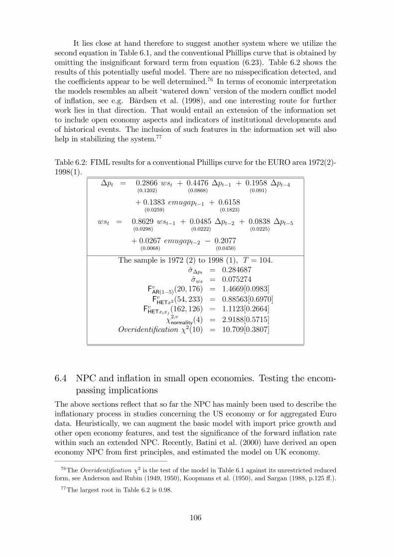
It lies close at hand therefore to suggest another system where we utilize thesecond equation in Table 6.1, and the conventional Phillips curve that is obtained byomitting the insignificant forward term from equation (6.23). Table 6.2 shows theresults of this potentially useful model. There are no misspecification detected, andthe coefficients appear to be well determined.76 In terms of economic interpretationthe models resembles an albeit ‘watered down’ version of the modern conflict modelof inflation, see e.g. Bårdsen et al. (1998), and one interesting route for furtherwork lies in that direction. That would entail an extension of the information setto include open economy aspects and indicators of institutional developments andof historical events. The inclusion of such features in the information set will alsohelp in stabilizing the system.77
Table 6.2: FIML results for a conventional Phillips curve for the EURO area 1972(2)-1998(1).
∆pt = 0.2866(0.1202)
wst + 0.4476(0.0868)
∆pt−1 + 0.1958(0.091)
∆pt−4
+ 0.1383(0.0259)
emugapt−1 + 0.6158(0.1823)
wst = 0.8629(0.0298)
wst−1 + 0.0485(0.0222)
∆pt−2 + 0.0838(0.0225)
∆pt−5
+ 0.0267(0.0068)
emugapt−2 − 0.2077(0.0450)
The sample is 1972 (2) to 1998 (1), T = 104.σ∆pt = 0.284687σws = 0.075274
FvAR(1−5)(20, 176) = 1.4669[0.0983]
FvHETx2(54, 233) = 0.88563[0.6970]FvHETxixj(162, 126) = 1.1123[0.2664]
χ2,vnormality(4) = 2.9188[0.5715]Overidentification χ2(10) = 10.709[0.3807]
6.4 NPC and inflation in small open economies. Testing the encom-passing implications
The above sections reflect that so far the NPC has mainly been used to describe theinflationary process in studies concerning the US economy or for aggregated Eurodata. Heuristically, we can augment the basic model with import price growth andother open economy features, and test the significance of the forward inflation ratewithin such an extended NPC. Recently, Batini et al. (2000) have derived an openeconomy NPC from first principles, and estimated the model on UK economy.
76The Overidentification χ2 is the test of the model in Table 6.1 against its unrestricted reducedform, see Anderson and Rubin (1949, 1950), Koopmans et al. (1950), and Sargan (1988, p.125 ff.).77The largest root in Table 6.2 is 0.98.
106
Once we consider the NPC for individual European economies, there are newpossibilities for testing–since preexisting results should, in principle, be explainedby the new model (the NPC). Specifically, in UK and Norway, the two economiesthat we investigate here, there exist models of inflation that build on a differentframework than the NPC, namely wage bargaining, monopolistic price setting andcointegration, see e.g., Nickell and Andrews (1983), Hoel and Nymoen (1988), Ny-moen (1989a) for early contributions, and Blanchard and Katz (1999) for a view onthis difference in modelling tradition in the US and Europe. Since the underlyingtheoretical assumptions are quite different for the two traditions, the existing em-pirical models define an information set that is wider than the set of instrumentsthat we have seen are typically employed in the estimation of NPCs. In particular,the existing studies claim to have found cointegrating relationships between levelsof wages, prices and productivity. These relationships constitute evidence that canbe used to test the implications of the NPC.
6.4.1 The encompassing implications of the NPC
Already there is a literature on the testing of feed-forward (rational expectationsbased) and feed-back models (allowing data based expectation formation), see Hendry(1988), Engle and Hendry (1993) and Ericsson and Hendry (1999). One of the in-sights is that the rational expectations hypothesis is inconsistent with the jointfinding of a stable feed-back model and a regime shift in the process driving theexplanatory variable (i.e., xt above). Essentially, an implication of the feed-forwardmode, namely that the Lucas critique applies in the described situation, is refutedby the stability of the feed-back model in the presence of a regime shift.
The test below builds on the same type of logic, namely that certain testableimplications follow from the premise that the NPC (with rational expectations) isthe correct model. Specifically, the following procedure is suggested78:
1. Assume that there exists a set of variables z =£z1 z2
¤, where the sub-set z1
is sufficient for overidentification of the maintained NPC model. The variablesin z2 are defined by the empirical findings of existing studies.
2. Using z1 as instruments, estimate the augmented model
∆pt = βfp1Et∆pt+1 + βbp1∆pt−1 + βp2xt + ...+ z2,t βp4
under the assumption of rational expectations about forward prices.
3. Under the hypothesis that the NPC is the correct model, βp4 = 0 is implied.Thus, non-rejection of the null hypothesis of βp4 = 0, corroborates the feed-forward Phillips curve. In the case of the other outcome: non-rejection ofβfp1 = 0, while βp4 = 0 is rejected statistically, the encompassing implicationof the NPCs refuted.
The procedure is clearly related to significance testing of the forward term, butthere are also notable differences. As mentioned above, the motivation of the test
78We thank David F. Hendry for suggesting this test to us.
107

is that of testing the implication of the rational expectations hypothesis, see Faveroand Hendry (1992) and Ericsson and Irons (1995). Thus, we utilize that under theassumption that the NPC is the correct model, consistent estimation of βfp1 can bebased on z1, and supplementing the set of instruments by z2 should not significantlychange the estimated βfp1.
In terms of practical implementation, we take advantage of the existing resultson wage and price modelling using cointegration analysis which readily imply z2-variables in the form of linear combinations of levels variables. In other wordsthey represent “unused” identifying instruments that goes beyond the informationset used in the Phillips curve estimation. Importantly, if agents are rational asassumed, this extension of the information set should not take away the significanceof ∆pet+1 in the NPC.
6.4.2 Norway
Consider the NPC (with forward term only) estimated on quarterly Norwegiandata:79
∆pt = 1.06(0.11)
∆pt+1 + 0.01(0.02)
wst + 0.04(0.02)
∆pbt + dummies(6.29)
χ2J (10) = 11.93 [0.29] .
The closed economy specification has been augmented heuristically with import pricegrowth (∆pbt) and dummies for seasonal effects as well as the special events in theeconomy described in Bårdsen et al. (2002). Estimation is by GMM for the period1972.4 - 2001.1. The instruments used (i.e., the variables in z1) are lagged wagegrowth (∆wt−1, ∆wt−2), lagged inflation (∆pt−1, ∆pt−2), lags of level and change inunemployment (ut−1, ∆ut−1, ∆ut−2), and changes in energy prices (∆pet, ∆pet−1),the short term interest rate (∆RLt, ∆RLt−1) and the length of the working day(∆ht).
The coefficient estimates are similar to GG. Strictly speaking, the coefficientof E[∆pt+1 | It] suggests that a backward solution is appropriate. But more impor-tantly the estimated NPC once more appears to be a modified random walk model.We checked the stability of the key parameters of the model by rolling regressionswith a fixed window of 85 observations. Figure 6.5 can be compared with Figure 6.2for the Euro area showing that the sample dependency is more pronounced in thecase of Norway. That said, the standard errors of the estimates are smaller in thiscase.
79Inflation is measured by the official consumer price index, see Appendix B.
108
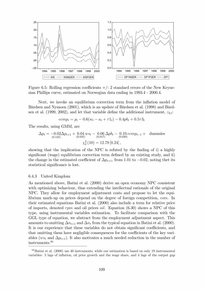
-.05
.00
.05
.10
.15
.20
.25
1994 1995 1996 1997 1998 1999 2000
WS WSM2ER WSP2ER
0.0
0.2
0.4
0.6
0.8
1.0
1.2
1994 1995 1996 1997 1998 1999 2000
DP1M2ER DP1P2ER DP1
Figure 6.5: Rolling regression coefficients +/- 2 standard errors of the New Keyne-sian Phillips curve, estimated on Norwegian data ending in 1993.4 - 2000.4.
Next, we invoke an equilibrium correction term from the inflation model ofBårdsen and Nymoen (2001), which is an update of Bårdsen et al. (1998) and Bård-sen et al. (1999, 2002), and let that variable define the additional instrument, z2,t:
ecmpt = pt − 0.6(wt − at + τ1t)− 0.4pbt + 0.5τ3tThe results, using GMM, are
∆pt = −0.02(0.125)
∆pt+1 + 0.04(0.025)
wst − 0.06(0.017)
∆pbt − 0.10(0.020)
ecmpt−1 + dummies
χ2J (10) = 12.78 [0.24] ,
showing that the implication of the NPC is refuted by the finding of i) a highlysignificant (wage) equilibrium correction term defined by an existing study, and ii)the change in the estimated coefficient of ∆pt+1, from 1.01 to −0.02, noting thet itsstatistical significance is lost.
6.4.3 United Kingdom
As mentioned above, Batini et al. (2000) derive an open economy NPC consistentwith optimizing behaviour, thus extending the intellectual rationale of the originalNPC. They allow for employment adjustment costs and propose to let the equi-librium mark-up on prices depend on the degree of foreign competition, com. Intheir estimated equations Batini et al. (2000) also include a term for relative priceof imports, denoted rpm and oil prices oil. Equation (6.30) shows a NPC of thistype, using instrumental variables estimation. To facilitate comparison with theGGL type of equation, we abstract from the employment adjustment aspect. Thisamounts to omitting∆nt+1 and∆nt from the typical equation in Batini et al. (2000).It is our experience that these variables do not obtain significant coefficients, andthat omitting them have negligible consequences for the coefficients of the key vari-ables (wst and ∆pt+1). It also motivates a much needed reduction in the number ofinstruments.80
80Batini et al. (2000) use 40 instruments, while our estimation is based on only 19 instrumentalvariables: 5 lags of inflation, oil price growth and the wage share, and 4 lags of the output gap
109
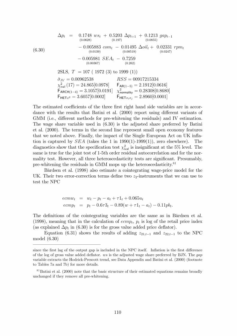
∆pt = 0.1748(0.0628)
wst + 0.5203(0.197)
∆pt+1 + 0.1213(0.0855)
gapt−1
− 0.005883(0.0139)
comt − 0.01495(0.00519)
∆oilt + 0.02331(0.0247)
rpmt
− 0.005981(0.00367)
SEAt − 0.7259(0.262)
(6.30)
2SLS, T = 107 ( 1972 (3) to 1999 (1))
σIV = 0.00962538 RSS = 00917215334χ2ival (17) = 24.865[0.0978] FAR(1−5) = 2.1912[0.0616]FARCH(1−4) = 3.1057[0.0191] χ2normality = 0.28308[0.8680]FHETx2 = 3.6057[0.0002] FHETxixj = 2.8960[0.0001]
The estimated coefficients of the three first right hand side variables are in accor-dance with the results that Batini et al. (2000) report using different variants ofGMM (i.e., different methods for pre-whitening the residuals) and IV estimation.The wage share variable used in (6.30) is the adjusted share preferred by Batiniet al. (2000). The terms in the second line represent small open economy featuresthat we noted above. Finally, the impact of the Single European Act on UK infla-tion is captured by SEA (takes the 1 in 1990(1)-1999(1)), zero elsewhere). Thediagnostics show that the specification test χ2ival is insignificant at the 5% level. Thesame is true for the joint test of 1-5th order residual autocorrelation and for the nor-mality test. However, all three heteroscedasticity tests are significant. Presumably,pre-whitening the residuals in GMM mops up the heteroscedasticity.81
Bårdsen et al. (1998) also estimate a cointegrating wage-price model for theUK. Their two error-correction terms define two z2-instruments that we can use totest the NPC
ecmwt = wt − pt − at + τ1t + 0.065ut
ecmpt = pt − 0.6τ3t − 0.89(w + τ1t − at)− 0.11pbt.
The definitions of the cointegrating variables are the same as in Bårdsen et al.(1998), meaning that in the calculation of ecmpt, pt is log of the retail price index(as explained ∆pt in (6.30) is for the gross value added price deflator).
Equation (6.31) shows the results of adding z21,t−1 and z22,t−1 to the NPCmodel (6.30)
since the first lag of the output gap is included in the NPC itself. Inflation is the first differenceof the log of gross value added deflator. ws is the adjusted wage share preferred by BJN. The gapvariable extracts the Hodrick-Prescott trend, see Data Appendix and Batini et al. (2000) (footnoteto Tables 7a and 7b) for more details.81Batini et al. (2000) note that the basic structure of their estimated equations remains broadly
unchanged if they remove all pre-whitening.
110
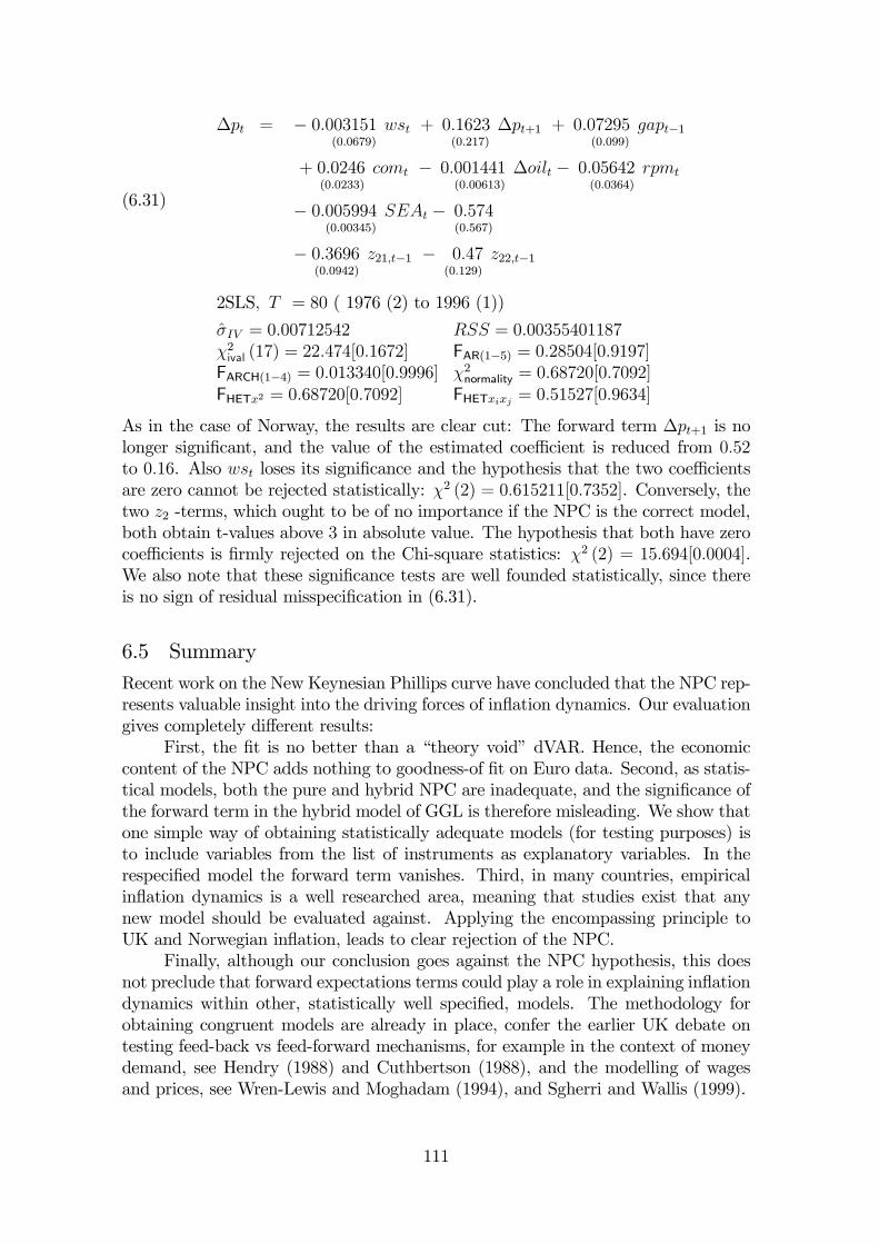
∆pt = − 0.003151(0.0679)
wst + 0.1623(0.217)
∆pt+1 + 0.07295(0.099)
gapt−1
+ 0.0246(0.0233)
comt − 0.001441(0.00613)
∆oilt − 0.05642(0.0364)
rpmt
− 0.005994(0.00345)
SEAt − 0.574(0.567)
− 0.3696(0.0942)
z21,t−1 − 0.47(0.129)
z22,t−1
(6.31)
2SLS, T = 80 ( 1976 (2) to 1996 (1))
σIV = 0.00712542 RSS = 0.00355401187χ2ival (17) = 22.474[0.1672] FAR(1−5) = 0.28504[0.9197]FARCH(1−4) = 0.013340[0.9996] χ2normality = 0.68720[0.7092]FHETx2 = 0.68720[0.7092] FHETxixj = 0.51527[0.9634]
As in the case of Norway, the results are clear cut: The forward term ∆pt+1 is nolonger significant, and the value of the estimated coefficient is reduced from 0.52to 0.16. Also wst loses its significance and the hypothesis that the two coefficientsare zero cannot be rejected statistically: χ2 (2) = 0.615211[0.7352]. Conversely, thetwo z2 -terms, which ought to be of no importance if the NPC is the correct model,both obtain t-values above 3 in absolute value. The hypothesis that both have zerocoefficients is firmly rejected on the Chi-square statistics: χ2 (2) = 15.694[0.0004].We also note that these significance tests are well founded statistically, since thereis no sign of residual misspecification in (6.31).
6.5 SummaryRecent work on the New Keynesian Phillips curve have concluded that the NPC rep-resents valuable insight into the driving forces of inflation dynamics. Our evaluationgives completely different results:
First, the fit is no better than a “theory void” dVAR. Hence, the economiccontent of the NPC adds nothing to goodness-of fit on Euro data. Second, as statis-tical models, both the pure and hybrid NPC are inadequate, and the significance ofthe forward term in the hybrid model of GGL is therefore misleading. We show thatone simple way of obtaining statistically adequate models (for testing purposes) isto include variables from the list of instruments as explanatory variables. In therespecified model the forward term vanishes. Third, in many countries, empiricalinflation dynamics is a well researched area, meaning that studies exist that anynew model should be evaluated against. Applying the encompassing principle toUK and Norwegian inflation, leads to clear rejection of the NPC.
Finally, although our conclusion goes against the NPC hypothesis, this doesnot preclude that forward expectations terms could play a role in explaining inflationdynamics within other, statistically well specified, models. The methodology forobtaining congruent models are already in place, confer the earlier UK debate ontesting feed-back vs feed-forward mechanisms, for example in the context of moneydemand, see Hendry (1988) and Cuthbertson (1988), and the modelling of wagesand prices, see Wren-Lewis and Moghadam (1994), and Sgherri and Wallis (1999).
111
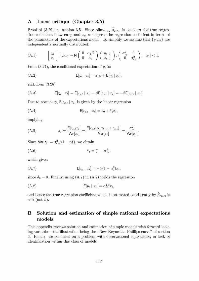
A Lucas critique (Chapter 3.5)
Proof of (3.29) in section 3.5. Since plimT→∞ βOLS is equal to the true regres-sion coefficient between yt and xt, we express the regression coefficient in terms ofthe parameters of the expectations model. To simplify we assume that {yt,xt} areindependently normally distributed:
(A.1)·ytxt
¸| It−1 ∼ N
µ0 α1β0 α1
¶µyt−1xt−1
¶,
µσ2
y0
0 σ2x
¶, |α1| < 1.
From (3.27), the conditional expectation of yt is:
(A.2) E[yt | xt] = xtβ + E[ηt | xt],
and, from (3.28):
(A.3) E[ηt | xt] = E[ y,t | xt]− βE[ x,t | xt] = −βE[ x,t | xt].
Due to normality, E[ x,t | xt] is given by the linear regression
(A.4) E[ x,t | xt] = δ0 + δ1xt,
implying
(A.5) δ1 =E[ x,txt]
Var[xt]=E[ x,t(α1xt−1 + x,t)]
Var[xt]=
σ2x
Var[xt].
Since Var[zt] = σ2x/(1− α21), we obtain
(A.6) δ1 = (1− α21),
which gives:
(A.7) E[ηt | xt] = −β(1− α21)xt,
since δ0 = 0. Finally, using (A.7) in (A.2) yields the regression
(A.8) E[yt | xt] = α21βxt,
and hence the true regression coefficient which is estimated consistently by βOLS isα21β (not β).
B Solution and estimation of simple rational expectationsmodels
This appendix reviews solution and estimation of simple models with forward look-ing variables–the illustration being the “New Keynesian Phillips curve” of section6. Finally, we comment on a problem with observational equivalence, or lack ofidentification within this class of models.
112
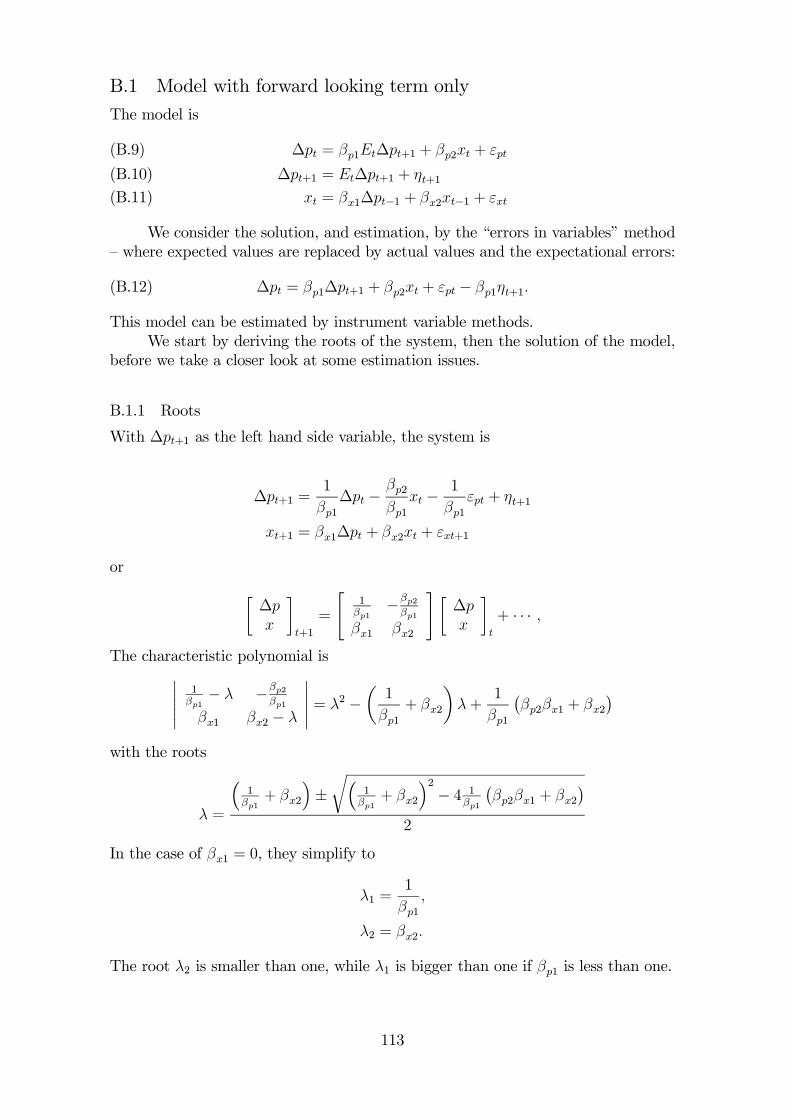
B.1 Model with forward looking term onlyThe model is
∆pt = βp1Et∆pt+1 + βp2xt + εpt(B.9)
∆pt+1 = Et∆pt+1 + ηt+1(B.10)
xt = βx1∆pt−1 + βx2xt−1 + εxt(B.11)
We consider the solution, and estimation, by the “errors in variables” method— where expected values are replaced by actual values and the expectational errors:
(B.12) ∆pt = βp1∆pt+1 + βp2xt + εpt − βp1ηt+1.
This model can be estimated by instrument variable methods.We start by deriving the roots of the system, then the solution of the model,
before we take a closer look at some estimation issues.
B.1.1 Roots
With ∆pt+1 as the left hand side variable, the system is
∆pt+1 =1
βp1∆pt −
βp2βp1
xt − 1
βp1εpt + ηt+1
xt+1 = βx1∆pt + βx2xt + εxt+1
or ·∆px
¸t+1
=
"1βp1
−βp2βp1
βx1 βx2
#·∆px
¸t
+ · · · ,
The characteristic polynomial is¯¯ 1
βp1− λ −βp2
βp1
βx1 βx2 − λ
¯¯ = λ2 −
µ1
βp1+ βx2
¶λ+
1
βp1
¡βp2βx1 + βx2
¢with the roots
λ =
³1βp1+ βx2
´±r³
1βp1+ βx2
´2− 4 1
βp1
¡βp2βx1 + βx2
¢2
In the case of βx1 = 0, they simplify to
λ1 =1
βp1,
λ2 = βx2.
The root λ2 is smaller than one, while λ1 is bigger than one if βp1 is less than one.
113
B.1.2 Solution
Consider the simplified system with βx1 = 0:
∆pt = βp1∆pt+1 + βp2xt + εpt − βp1ηt+1
xt+1 = βx2xt + εxt+1
Following Davidson (2000, p. 109—10), we derive the solution in two steps:
1. Find Et∆pt+1
2. Solve for ∆pt
Solving for Et∆pt+1 We start by reducing the model to a single equation:
∆pt = βp1∆pt+1 + βp2βx2xt−1 + βp2εxt + εpt − βp1ηt+1.
Solving forwards then produces:
∆pt = βp1¡βp1∆pt+2 + βp2βx2xt + βp2εxt+1 + εpt+1 − βp1ηt+2
¢+βp2βx2xt−1+βp2εxt+εpt−βp1ηt+1
=¡βp2βx2xt−1 + βp2εxt + εpt − βp1ηt+1
¢+βp1
¡βp2βx2xt + βp2εxt+1 + εpt+1 − βp1ηt+2
¢+¡βp1¢2∆pt+2
=nX
j=0
¡βp1¢j ¡
βp2βx2xt+j−1 + βp2εxt+j + εpt+j − βp1ηt+j+1¢+¡βp1¢n+1
∆pt+n+1.
By imposing the transversality condition:
limn→∞
¡βp1¢n+1
∆pt+n+1 = 0
and then taking expectations conditional at time t, we get the “discounted solution”:
Et∆pt+1 =∞Xj=0
¡βp1¢j ¡
βp2βx2Etxt+j + βp2Etεxt+j+1 +Etεpt+j+1 − βp1Etηt+j+2¢
=∞Xj=0
¡βp1¢j ¡
βp2βx2Etxt+j¢.
However, we know the process for the forcing variable, so:
Et−1xt = βx2xt−1Etxt = xt
Etxt+1 = βx2xt
Etxt+2 = Et (Et+1xt+2) = Etβx2xt+1 = β2x2xt
Etxt+j = βjx2xt.
We can therefore substitute in:
114
Et∆pt+1 =∞Xj=0
¡βp1¢j ¡
βp2βx2βjx2xt
¢= βp2βx2
∞Xj=0
¡βp1βx2
¢jxt
=
µβp2βx2
1− βp1βx2
¶xt
All that is left to obtain the complete solution is to substitute back into theoriginal equation and rearrange.
Solving for ∆pt
∆pt = βp1Et∆pt+1 + βp2xt + εpt
= βp1
µβp2βx2
1− βp1βx2
¶xt + βp2xt + εpt
=
µβp2
1− βp1βx2
¶xt + εpt
B.1.3 Estimation
The implications of estimating the model by means of the “errors in variables”method is to induce moving average errors. Following Blake (1991), this can bereadily seen as follows:
1. Lead (B.9) one period and subtract the expectation to find the RE error:
ηt+1 = ∆pt+1 − Et∆pt+1
= βp1Et+1∆pt+2 + βp2xt+1 + εpt+1 −Et∆pt+1
=
µβp2
1− βp1βx2
¶xt+1 + εpt+1 −
µβp2
1− βp1βx2
¶βx2xt
= εpt+1 +
µβp2
1− βp1βx2
¶εxt+1
2. Substitute into (B.12):
∆pt = βp1∆pt+1 + βp2xt + εpt − βp1εpt+1 −µ
βp1βp21− βp1βx2
¶εxt+1.
So even though the original model has white noise errors, the estimated modelwill have first order moving average errors.
115
B.2 Hybrid model with both forward and backward looking termsThe model is now
∆pt = βfp1Et∆pt+1 + βbp1∆pt−1 + βp2xt + εpt(B.13)
∆pt+1 = Et∆pt+1 + ηt+1(B.14)
xt = βx1∆pt−1 + βx2xt−1 + εxt(B.15)
B.2.1 Roots
With ∆pt+1 as the left hand side variable, the system is
∆pt+1 =1
βfp1∆pt −
βbp1
βfp1∆pt−1 −
βp2
βfp1xt − 1
βfp1εpt + ηt+1
xt+1 = βx1∆pt + βx2xt + εxt+1
with companion form ∆pt+1xt+1∆pt
= 1
βfp1−βp2
βfp1−βbp1
βfp1
βx1 βx2 01 0 0
∆pt
xt∆pt−1
+ · · · ,and characteristic polynomial
λ3 −Ã1
βfp1+ βx2
!λ2 +
1
βfp1
¡βbp1 + βbp1βx1 + βx2
¢λ− βbp1
βfp1βx2.
In the simplified case of βx1 = 0, the roots are
λ1 = βx2,
λ2 =121
βfp1
µ1−
q1− 4βbp1βfp1
¶,
λ3 =121
βfp1
µ1 +
q1− 4βbp1βfp1
¶.
With the further restriction βbp1 + βfp1 = 1, the roots simplify to
λ1 = βx2,λ2 =
1
βfp1− 1,
λ3 = 1.
B.3 Does the MA(1) process prove that the forward solution applies?Assume that the true model is
∆pt = βp1∆pt−1 + εpt,¯βp1¯< 1
116
but that the following model is estimated by instrument variable methods
∆pt = βfp1∆pt+1 + εfpt
What are the properties of εfpt?
εfpt = ∆pt − βfp1∆pt+1
Assume, as is common in the literature, that we find that βfp1 ≈ 1. Then
εfpt ≈ ∆pt −∆pt+1 = −∆2pt+1
= − £εpt+1 + (βp1 − 1)εpt + ...¤.
So we obtain a model with a moving average residual, but this time the reason isnot forward looking behaviour but rather model misspecification.
117
C Data used in Chapter 3-5
C.1 Annual data set for Norwegian manufacturing wages.All data are taken from the database on Nordic wage formation originally doc-umented (in Norwegian) by Evjen and Langset (1997). The data is available inPcGive format and excell on the following URL: Below we first give a general defi-nition of each variable used in the empirical sections of this paper. In brackets, wegive the variable’s name in Evjen and Langset’s database, and the algebra we haveused to transform each variable into the form it used in the estimated equations.
• w = log of wage costs per hour in manufacturing. [Source variable : WC,1970 = 100] : Transformation: w = ln(WC/100).]
• cpi = log of the consumer price index [Source variable: CPI, 1970 = 100,Transformation: p = ln(CPI/100)].
• q = log GDP deflator for manufacturing [Source variable: P , 1970 = 1. Trans-formation: q = ln(P/100)].
• a =log of average labour productivity in manufacturing [Source variable: PR,1970 = 100. Transformation: pr = ln(PR/100)].
• t1 = log of one plus the pay roll tax rate [Source variable: PT . Transformation:pt = ln(1 + PT ) ≈ PT ].
• t2 = log of one minus the income tax rate [Source variable: AT . Transforma-tion: at = ln(1−AT ) ≈ AT ].
• pq = wedge (= pt− at+ p− q).
• h = log of normal weekly working hours. [Source variable: Norway: HR, h =ln(H) ]rpr = log of replacement rate [Source variable: RPR. Transformation:rpr =ln(RPR)].
• u = log of open unemployment (registered unemployed) in per cent of labourforce [Source variable: U . Transformation: u = ln(U/100)].
• tu =log of total unemployment (registered unemployed plus participants inactive labour market programmes) in per cent of labour force [Source variable:U . Transformation: u = ln(TUPR/100)]
• lmp = log of one minus the per cent of total unemployed who are participat-ing in active labour market programmes. Yearly average.[Source: AMUN .Transformation: lmp = ln(1−AMUN/100)].
• IP = Dummy for income policy in Norway. 1 in 1979. 0.5 in 1980. 1 in 1988and 0.5 in 1989.
118
C.2 United Kingdom, quarterly wage and price data.All variables are seasonally adjusted except for the RPI. ONS is the Office for Na-tional Statistics (formerly the CSO).
W Wages: index of actual quarterly average earnings: ONS identifier DNAB.
P Retail Price Index: ONS identifier: CHAW.
PR Non-north sea productivity: ONS identifiers: CKJL/DYDC.
PI Price deflator for expenditure on imported goods and services: ONS identifiers:DJBC/DJDJ.
U Unemployment rate, registered number of unemployed: ONS identifier: BCJE.
gap Output gap defined as log of non-north sea GDP (NNO) deviations from trend,where the trend is estimated by the Hodrick-Prescott filter using λ = 1600.ONS identifier for NNO: CKJL.
T1 Employers tax rate: (GTAY + AIIR + TSET )/(34.203 ∗DNAB ∗ (BCAD +BCAH)/1000) which are ONS identifiers apart from TSET which is receiptsof selective employment tax. GTAY andAIIR give employers’ National Insur-ance and other contributions and the last term gives the aggregate employedsalary bill.
T3 Tax rate on the retail price index basket, excl. mortgage interest payments. Thistax rate is derived from the Bank of England’s spreadsheet for construction ofRPIY (see Beaton and Fisher (1995)).
BONUS Impulse dummy for retimed bonus payments brought forward one monthbefore a General Election. Takes the value 1 in 1992:1 and -1 in 1992:2.
IP4 Incomes policy dummy. Zero after 1979:2: source Whitley (1986).
D Data used in used in section 6
D.1 The Euroland data
D.1.1 The basic series from ECB
The data for Euroland is derived from a set of data base for the Area Wide modelof the ECB, see Fagan et al. (2001), which can be downloaded with the paper athttp://www.ecb.int/. The following series are used from that data base:YEN - Nominal GDP.YER - Real GDP.WIN - Compensation to employees.LNN - Total employment.
119
YGA - Output gap, defined as actual real output relative to potential real output(YET) measured by a constant returns to scale production function with neutraltechnical progress.
D.1.2 Data used to replicate GGL (sections 6.1 and 6.3.1)
pt = 100 · log(Y EN/Y ER) - GDP price level.wst = 100 · (log(WIN/(Y EN · 6.1333333))−mean(log(WIN/(Y EN · 6.1333333))- Wage share corrected for a constant (due to Sbordone (2002)) minus the samplemean of this corrected wage share.gapt = Output gap, defined as the deviation of log of the actual real output(100·log(YER)) from a quadratic trend.wt = 100·log(WIN/LNN) - wages. The annualised growth in wages (4·(wt−wt−1))is used as an instrument by GGL.
D.1.3 Data used in sections 6.3.3 - 6.3.5
emugapt = 100 · (Y GA− 1).
D.2 The U.S. data
D.2.1 The source data
PGDP = Total GDP chain index (1996=100).GDP = Real GDP, total U.S. economy.
Sources: U.S. National Income accounts.For later use:
COMPHR = Hourly Non-Farm Business (NFB) compensation.LABSHR= Labour share in Non-Farm Business (NFB) income.
Sources: LABSHR and COMPHR is from Bureau of Labor Statistics’ Produc-tivity and Cost release.
D.2.2 Data used in section 6.3.1
pt = log(PGDP ).gapt = Output gap, defined as the deviation of the log of actual real GDP output(log(GDPt)) from a quadratic trend.
For later use:wst = log(LABSHR)− log(mean) - Demeaned labour share.
D.3 The Norwegian data
D.3.1 Notes
1. Unless another source is given, all data are taken from RIMINI, the quarterlymacroeconometric model used in Norges Bank (The Central Bank of Norway).The data are seasonally unadjusted.
120
2. For each RIMINI-variable, the corresponding name in the RIMINI-databaseis given by an entry [RIMINI: variable name] at the end of the description.(The RIMINI identifier is from Rikmodnotat 140, Version 3.1415, dated 11.December 2001, Norges Bank, Research Department.)
3. Several of the variables refer to the mainland economy, defined as total econ-omy minus oil and gass production and international shipping.
4. Baseyear is 1997 (for the sample 1972.4 - 2001.1).
D.3.2 Definitions
H Normal working hours per week (for blue and white colour workers). [RIMINI:NH].
P Consumer price index. Baseyear =1. [RIMINI: CPI].
PB Deflator of total imports. Baseyear =1. [RIMINI: PB].
PE Consumer price index for electricity. Baseyear = 1 [RIMINI: CPIEL].
PR Mainland economy value added per man hour at factor costs, fixed baseyear(1991) prices. Mill. NOK. [RIMINI: ZYF].
RL Average interest rate on bank loans. [RIMINI: R.LB].
τ1 Employers tax rate. τ1 =WCF/WF − 1.τ3 Indirect tax rate. [RIMINI: T3].
U Rate of unemployment. registered unemployed plus persons on active labourmarket programmes as a percentage of the labour force, calculated as employedwage earners plus unemployment. [RIMINI: UTOT].
W Nominal mainland hourly wages. This variable is constructed from RIMINI-database series as a weighted average of hourly wages in manufactures andconstruction and hourly wages in private and public service production, withtotal number of man-hours (corrected for vacations, sick hours, etc) as weights:
W = (WIBA ∗ TWIBA+WOTV J ∗ (TWTV + TWO + TWJ))/TWF.
Finally, the NPC model (6.29) for Norway includes seasonal dummies and
Pdum Composite dummy for introduction and lift of direct price regulations. 1 in1971.1, 1971.2,1976.4,1977.4, 1979.1,1996.1. -1 in 1975.1,1980.1,1981.1,1982.1,1986.3. Zero otherwise.
121
D.4 The UK data
D.4.1 The source data for the Bank of England study
Batini et al. (2000) use the following series from UK Office of National Statistics:ABML - Gross value added at basic prices (excluding taxes less subsidies on prod-ucts).ABMM - Gross value added (constant prices) at basic prices.AJFA - British pounds - US dollar exchange rate.BCAJ - Number of employee in the work-force (seasonally adjusted).DYZN - Number of selfemployment work-force jobs (seasonally adjusted).HAEA - Compensation to employees, including the value of social contributionspayable by the employer.IKBI - Total imports (to the UK) at current prices.IKBL - Total imports (to the UK) at constant prices.NMXS - Compensation of employees paid by general government.
Moreover, Batini et al. (2000) calculate and collect from other sources:GGGVA - A measure of the part of gross value added attributable to general gov-ernment.PETSPOT - Oil spot price (average of Brent Crude, West Texas and Dubai Light).Source: Bloomberg.WPX - Weighted average of export prices from the G7 countries (excluding UK),with effective exchange rates as weights. Sources: Datastream and InternationalFinance Statistics, IMF.EER - UK nominal effective exchange rate. Source: International Finance Statistics,IMF.A = (BCAJ + DYZN) / BCAJ
D.4.2 Bank of England variables used in section 6.4.3
Small letters denote natural logarithms (log) :wst = log[{((HAEAt −NMXSt) ·At)/(ABMLt −GGGVAt)} · 100].pt = log[(ABMLt/ABMMt) · 100].oilt = log[PETSPOTt/AJFAt) · 100].gapt = Output gap defined as output (log(ABMMt)) deviations from trend, wherethe trend is estimated by a Hodrick-Prescott filter.comt = log[(WPXt/EERt) · 100].rpmt = log[(IKBIt/IKBLt) · 100].nt = log(BCAJt +DY ZNt)SEAt = Dummy variable for the Single European Act, which takes on the value 1after 1990.1, zero otherwise.
D.4.3 Variables used to calculate the error correction terms in section 6.4.3
Wt− Wages, index of actual quarterly earnings.Pt− Retail price index.PRt− Non -North Sea productivity.
122
PBt− Price deflator for expenditure on imported goods and services.Ut− Unemployment rate: registered number of unemployed.τ1t− Employers’ tax rate.τ3t− Tax rate on the retail price index basket, excluding mortgage interest pay-ments.
For more precise definitions and for sources, see Bårdsen et al. (1998).
References
Alogoskoufis, G. S. and A. Manning (1988). On the Persistence of Unemployment.Economics Policy.
Andersen, T. M. (1994). Price Rigidity. Causes and Macroeconomic Implications.Claredon Press, Oxford.
Anderson, T. W. and H. Rubin (1949). Estimation of the parameters of a singleequation in a complete system of stochastic equations. Annals of MathematicalStatistics, 20 , 46—63.
Anderson, T. W. and H. Rubin (1950). The asymptotic properties of estimates ofthe parameters of a single equation in a complete system of stochastic equations.Annals of Mathematical Statistics, 21 , 570—582.
Apel, M. and P. Jansson (1999). System Estimates of Potential Output and theNAIRU. Empirical Economics, 24 , xxx—xxxx.
Aukrust, O. (1977). Inflation in the Open Economy. A Norwegian Model. In Klein,L. B. andW. S. Sâlant (eds.),World Wide Inflation. Theory and recent experience.Brookings, Washington D.C.
Backhouse, R. E. (1995). Interpreting Macroeconomics. Explorations in the Historyof Macroeconomic Thought . Routledge, London and New York.
Backhouse, R. E. (2000). Theory, Evidence and the Labour Market. In Backhouse,R. E. and A. Salanti (eds.), Macroeconomics and the Real World. Volume 2:Keynesian Economics, Unemployment and Policy, chap. 7A, 145—155. OxfordUniversity Press, Oxford.
Bank of England (1999). Economic Models at the Bank of England . Bank of England,London.
Bårdsen, G. and P. G. Fisher (1999). Economic Theory and Econometric Dynamicsin Modelling Wages and Prices in the United Kingdom. Empirical Economics,24 (3), 483—507.
Bårdsen, G., P. G. Fisher and R. Nymoen (1998). Business Cycles: Real Facts orFallacies? In Strøm, S. (ed.), Econometrics and Economic Theory in the 20th Cen-tury: The Ragnar Frisch Centennial Symposium, no. 32 in Econometric SocietyMonograph Series, chap. 16, 499—527. Cambridge University Press, Cambridge.
123
Bårdsen, G., E. S. Jansen and R. Nymoen (1999). Econometric Inflation Target-ing. Arbeidsnotat 1999/5, Research Department, Norges Bank [Central Bank ofNorway].
Bårdsen, G., E. S. Jansen and R. Nymoen (2002). Model specification and inflationforecast uncertainty. Annales d’Économie et de Statistique, 67 (68), 495—517.
Bårdsen, G. and R. Nymoen (2001). Sammenhengen mellom rente og inflasjon(Interest rates and inflation). Norsk Økonomisk Tidsskrift , 115(2), 125—147.
Bårdsen, G. and R. Nymoen (2003). Testing Steady-State Implications for theNAIRU. Review of Economics and Statistics. Forthcoming.
Barkbu, B. B., R. Nymoen and K. Røed (2002). Wage Coordination and Unemploy-ment Dynamics in Norway and Sweden. Journal of Socio-Economics. Forthcom-ing.
Batini, N., B. Jackson and S. Nickell (2000). Inflation dynamics and the labourshare in the UK. Discussion Paper 2, External MPC Unit, Bank of England.
Bean, C. (1994). European unemployment: A survey. Journal of Economic Litera-ture, XXXII , 573—619.
Beaton, R. and P. G. Fisher (1995). The Construction of RPIY. Working PaperSeries 28, Bank of England.
Bjerkholt, O. (1998). Interaction between model builders and policy makers in theNorwegian tradition. Economic Modelling, 15 , 317—339.
Blake, D. (1991). The Estimation of Rational Expectations Models: A survey.Journal of Economic Studies, 18(3), 31—70.
Blanchard, O. J. (1987). The Wage Price Spiral. Quarterly Journal of Economics,101 , 543—565.
Blanchard, O. J. and S. Fisher (1989). Lectures on Macroeconomics. The MITPress, Cambridge, Massachusets.
Blanchard, O. J. and L. Katz (1997). What Do We Know and Do Not Know Aboutthe Natural Rate of Unemployment. Journal of Economic Perspectives, 11 , 51—72.
Blanchard, O. J. and L. Katz (1999). Wage Dynamics: Reconciling Theory andEvidence. NBER Working Paper Series 6924, National Bureau of Economic Re-search.
Blanchard, O. J. and N. Kiyotaki (1987). Monopolistic Competition and the Effectsof Aggregate Demand. American Economic Review , 77 , 647—666.
Blanchard, O. J. and L. H. Summers (1986). Husteresis and the European Unem-ployment Problem. NBER Macroeconomics Manual , 1 , 15—78.
Blanchflower, D. G. and A. J. Oswald (1994). The Wage Curve. The MIT Press,Cambridge, Massachusetts.
124
Brockwell, P. J. and R. A. Davies (1991). Time Series: Theory and Methods. Secondedition.. Springer, New York.
Bruno, M. (1979). Price and Output Adjustment: Micro Foundations and MacroTheory. Journal of Monetary Economics, 5 , 187—212.
Bruno, M. and J. Sachs (1984). Economics of World Wide Stagflation. Basil Black-well, Oxford.
Calmfors, L. (1977). Inflation in Sweden. In Klein, L. B. and W. S. Sâlant (eds.),World Wide Inflation. Theory and recent experience. Brookings, Washington D.C.
Calmfors, L. and A. Forslund (1991). Real-Wage Determination and Labour MarketPolicies: The Swedish Experience. The Economic Journal , 101 , 1130—1148.
Calmfors, L. and R. Nymoen (1990). Nordic Employment. Economic Policy, 5 (11),397—448.
Calvo, G. A. (1983). Staggered prices in a utility maximizing framework. Journalof Monetary Economics, 12 , 383—398.
Carlin, W. and D. Soskice (1990). Macroeconomics and the Wage Bargain. OxfordUniversity Press, Oxford.
Carruth, A. A. and A. J. Oswald (1989). Pay Determination and Industrial Pros-perity. Oxford University Press, Oxford.
Cassino, V. and R. Thornton (2002). Do Changes in Structural Factors ExplainMovements in the Equilibirum Rate of Unemployment? Working paper, Bank ofEngland.
Chadha, B., P. R. Masson and G. Meredith (1992). Models of Inflation and theCosts of Disinflation. IMF Staff Papers, 39 , 395—431.
Chow, G. C. (1960). Tests of equality between sets of coefficients in two linearregressions. Econometrica, 28 , 591—605.
Clarida, R., J. Galí and M. Gertler (1999). The Science of Monetary Policy: A NewKeynesian Perspective. Journal of Economic Literature, 37 (4), 1661—1707.
Clements, M. P. and D. F. Hendry (1996). Intercept Corrections and StructuralBreaks. Journal of Applied Econometrics, 11 , 475—494.
Clements, M. P. and D. F. Hendry (1998). Forecasting Economic Time Series.Cambridge University Press, Cambridge.
Clements, M. P. and D. F. Hendry (1999). Forecasting Non-stationary EconomicTime Series. The MIT Press, Cambridge, MA.
Courbis, R. (1974). Liason Internationale Des Prix et Inflation Importé. economieappliquée, 27 , 205–220.
125
Cromb, R. (1993). A Survey of Recent Econometric Work on the NAIRU. Journalof Economic Studies, 20 (1/2), 27—51.
Cross, R. (ed.) (1988). Unemployment, Hysteresis and the Natural Rate Hypothesis.Basil Blackwell, Oxford.
Cross, R. (ed.) (1995). The Natural Rate of Unemployment . Basil Blackwell, Oxford.
Cuthbertson, K. (1988). The Demand for M1: A Forward Looking Buffer StockModel. Oxford Economic Papers, 40 , 110–131.
Dasgupta, A. K. (1985). Epochs of Economic Theory. Basil Blackwell, Oxford.
Davidson, J. (2000). Econometric Theory. Blackwell, Oxford.
Davies, E. P. and L. Schøtt-Jensen (1994). Wage and Price Dynamics in EU-Countries: Preliminary Empirical Estimates. European Monetary Institute.
Desai, M. (1984). Wages, Prices and Unemployment a Quarter of a Century afterthe Phillips Curve. In Hendry, D. F. and K. F. Wallis (eds.), Econometrics andQuantitative Econometrics, chap. 9. Basil Blackwell, Oxford.
Desai, M. (1995). The Natural Rate of Unemployment: A Fundamentalist KeynesianView , chap. 16, 346–361. Cambridge University Press.
Doornik, J. (1996). Testing Vector Autocorrelation and Heteroscedasticity in Dy-namic Models. Working paper, Nuffield College.
Doornik, J. A. and H. Hansen (1994). A Practical Test of Multivariate Normality.Unpublished paper, Nuffield College.
Doornik, J. A. and D. F. Hendry (1997). Modelling Dynamic Systems Using PcFiml9 for Windows. International Thomson Publishing, London.
Drèze, J. and C. R. Bean (eds.) (1990a). Europe’s Unemployment Problem; Intro-duction and Synthesis. MIT Press, Cambridge.
Drèze, J. and C. R. Bean (1990b). Europe’s Unemployment Problem; Introduc-tion and Synthesis. In Drèze, J. and C. R. Bean (eds.), Europe’s UnemploymentProblem, chap. 1. MIT Press, Cambridge.
Driehuis, W. and P. de Wolf (1976). A Sectoral Wage and Price Model for theNetherlands’ Economy. In Frisch, H. (ed.), Inflation in Small Countries, 283–339. Springer-Verlag, New York.
Dunlop, J. T. (1944). Wage Determination under Trade Unions. Reprints of Eco-nomic Classic, 1966. Augustus M. Kelley Publishers, New York.
Edgren, G., K. O. Faxén and C. E. Odher (1969). Wages, Growth and Distributionof Income. Swedish Journal of Economics, 71 , 133—60.
Eika, K. H., N. R. Ericsson and R. Nymoen (1996). Hazards in Implementing aMonetary Conditions Index. Oxford Bulletin of Economics and Statistics, 58(4),765—790.
126
Elmeskov, J. (1994). Nordic Unemployment in a European Perspective. SwedishEconomic Policy Review , 1(1-2 Autumn 1994), 27—70.
Elmeskov, J. and M. MacFarland (1993). Unemployment Persistence. OECD Eco-nomic Studies, (21), 59—88.
Engle, R. F. (1982). Autoregressive Conditional Heteroscedasticity with Estimatesof the Variance of United Kingdom Inflation. Econometrica, 50 , 987—1007.
Engle, R. F. and D. F. Hendry (1993). Testing Super Exogeneity and Invariance inRegression Models. Journal of Econometrics, 56 , 119—139.
Ericsson, N. R. and D. Hendry (1999). Encompassing and Rational Expectations:How Sequential Corroboration Can Imply Refutation. Empirical Economics,24 (1), 1–21.
Ericsson, N. R. and J. S. Irons (1995). The Lucas Critique in Practice: TheoryWithout Measurement. In Hoover, K. D. (ed.), Macroeconometrics: Develop-ments, Tensions and Prospects, chap. 8. Kluwer Academic Publishers.
Ericsson, N. R., E. S. Jansen, N. A. Kerbeshian and R. Nymoen (1997). Under-standing a Monetary Conditions Index. Unpublished paper, presented at xxx.
Evjen, S. and T. Langset (1997). Arbeidsledighet og tiltak i Norden. Dokumentasjonav nordiske makrodata. Kommer som Arbeidsnotat fra SNF Oslo.
Fagan, G., J. Henry and R. Mestre (2001). An area-wide model (AWM) for theEuro area. Working Paper 42, European Central Bank.
Fair, R. C. (2000). Testing the NAIRU model for the United States. Review ofEconomics and Statistics, LXXXII , 64—71.
Favero, C. A. and D. F. Hendry (1992). Testing the Lucas Critique: A Review.Econometric Reviews, 11 , 265—306.
Ferri, P. (2000). Wage Dynamics and The Phillips Curve. In Blackhouse, R. E.and A. Salanti (eds.), Macroeconomics and the Real World. Volume 2: KeynesianEconomics, Unemployment and Policy, chap. 5. Oxford University Press, Oxford.
Fieller, E. C. (1954). Some Problems in Interval Estimation. Journal of the RoyalStatistical Society, 16(2), 175–185. Series B.
Forslund, A. and O. Risager (1994). Wages in Sweden. New and Old Results. Memo1994-22, University of Aarhus, Institute of Economics.
Friedman, M. (1968). The Role of Monetary Policy. American Economic Review ,58 (1), 1—17.
Frisch, H. (1977). The Scandinavian Model of Inflation. A Generalization and Em-pirical Evidence. Atlantic Economic Journal , 5 , 1—14.
Fuhrer, J. C. (1995). The Phillips Curve is Alive and Well. New England EconomicReview , 41—56.
127
Fuhrer, J. C. (1997). The (un)importance of forward-looking behavior in pricespecifications. Journal of Money, Credit and Banking, 29 , 338—350.
Fuhrer, J. C. and G. A. Moore (1995). Inflation persistence. Quarterly Journal ofEconomics, 110 , 127—159.
Galí, J. and M. Gertler (1999). Inflation Dynamics: A Structural EconometricAnalysis. Journal of Monetary Economics, 44 (2), 233—258.
Galí, J., M. Gertler and J. D. López-Salido (2001a). European Inflation Dynamics.European Economic Review , 45 , 1237—1270.
Galí, J., M. Gertler and J. D. López-Salido (2001b). Notes on estimating the closedform of the hybrid new Phillips curve. Unpublished paper, CREI/New YorkUniversity/Bank of Spain.
Godfrey, L. G. (1978). Testing for higher order serial correlation when the regressorsinclude lagged dependent variables. Econometrica, 46 , 1303—1313.
Gordon, R. J. (1983). ’Credibility’ Vs. ’Mainstream’: Two Views of the InflationProcess. In Nordhaus, W. D. (ed.), Inflation: Prospects and Remedies, Alterna-tives for the 1980s. Center for National Policy, Washington.
Gordon, R. J. (1997). The Time-Varying NAIRU and its Implications for EconomicPolicy. Journal of Economic Perspectives, 11 (1), 11—32.
Gourieroux, C. and A. Monfort (1997). Time Series and Dynamic Models. Cam-bridge University Press, Cambridge, New York.
Granger, C. W. J. and P. Newbold (1974). Spurious regressions in econometrics.Journal of Econometrics, 2 , 111—120.
Granger, C. W. J. and P. Newbold (1986). Forecasting Economic Time Series.Academic Press, San Diego.
Gregory, A. M. and M. R. Veall (1985). Formulating Wald Tests of NonlinearRestrictions. Econometrica, 53(6), 1465–1468.
Grubb, D. (1986). Topics in the OECD Phillips Curve. Economic Journal , 96 ,55—79.
Hansen, B. E. (1992). Testing for Parameter Instability in Linear Models. Journalof Policy Modelling, 14 , 517—533.
Hansen, L. P. (1982). Large Sample Properties of Generalized Method of MomentsEstimators. Econometrica, 50 , 1029—1054.
Harvey, A. C. (1981). The Econometric Analysis of Time Series. Philip Allan,Oxford.
Hendry, D. (1983). Econometric Modelling: The Consumption Function in Retro-spect. Scottish Journal of Political Economy, 30 , 193—220.
128
Hendry, D. F. (1988). The Encompassing Implications of Feedback verus Feedfor-ward Mechanisms in Econometrics. Oxford Economic Papers, 40 , 132—149.
Hendry, D. F. (1995a). Dynamic Econometrics. Oxford University Press, Oxford.
Hendry, D. F. (1995b). Econometrics and Business Cycle Empirics. The EconomicJournal , 105 , 1622—1636.
Hendry, D. F. and H. M. Krolzig (2001). Automatic Econometric Model SelectionUsing PcGets 1.0 . Timberlake Consultants, London.
Hendry, D. F. and G. E. Mizon (1978). Serial correlation as a convenient simplifi-cation, not a nuisance: a comment on a study of the demand for money by theBank of England. Economic Journal , 88 , 549—563.
Hendry, D. F. and G. E. Mizon (1993). Evaluating dynamic econometric modelsby encompassing the VAR. In Phillips, P. C. B. (ed.), Models, Methods andApplications of Econometrics, 272—300. Basil Blackwell, Oxford.
Hoel, M. and R. Nymoen (1988). Wage Formation in Norwegian Manufacturing. AnEmpirical Application of a Theoretical Bargaining Model. European EconomicReview , 32 , 977—997.
Holden, S. (1990). Wage Drift in Norway: A Bargaining Approach. In Calmfors,L. (ed.), Wage Formation and Macroeconomic Policy in the Nordic Countries,chap. 7. Oxford University Press, Oxford. With comment by T. Eriksson and P.Skedinger.
Holden, S. and R. Nymoen (1998).
Holden, S. and R. Nymoen (2002). Measuring Structural Unemployment: NAWRUEstimates in the Nordic Countries. The Scandinavian Journal of Economics,104 (1), 87–104.
Johansen, K. (1995). Norwegian Wage Curves. Oxford Bulletin of Economics andStatistics, 57 , 229–247.
Kendall, M. G. and A. Stuart (1973). The Advanced Theory of Statistics: Voume2, Inference and Relationship.. Charles Griffin and Company, London. ThirdEdition.
King, M. (1998). The Employment Policy Institute’s Fourth Annual Lecture:Lessons from the UK labour market. BIS Review 103, Bank for InternationalSettlement.
Kolsrud, D. and R. Nymoen (1998). Unemployment and the Open Economy Wage-Price Spiral. Journal of Economic Studies, 25 , 450—467.
Koopmans, T. C., H. Rubin and R. B. Leibnik (1950). Measuring the equationsystems of dynamic economics. In Koopmans, T. C. (ed.), Statistical inferencein dynamic economic models, Cowles Commission Monograph 10, 53—237. Wiley,New York.
129
Kremers, J. J. M., N. R. Ericsson and J. J. Dolado (1992). The Power of Cointe-gration Tests. Oxford Bulletin of Economics and Statistics, 54 , 325—348.
Layard, R. and S. Nickell (1986). Unemployment in Britain. Economica, 53 , 121—166. Special issue.
Layard, R., S. Nickell and R. Jackman (1991). Unemployment . Oxford UniversityPress, Oxford.
Layard, R., S. Nickell and R. Jackman (1994). The Unemployment Crises. OxfordUniversity Press, Oxford.
Lindbeck, A. (1993). Unemployment and Macroeconomics. The MIT Press, Cam-bridge.
Lindé, J. (2001). Estimating New-Keynesian Phillips Curves on Data With Mea-surements Errors A Full Information Maximum Likelihood Approach. WorkingPaper Series 129, Sveriges Rikbank.
Lipsey, R. G. (1960). The Relationship Between Unemployment and the Rate ofChange in Money Wages in the United Kingdom 1862-1957: a Further Analysis.Economica, 27 , 1—31.
Lucas, R. E., Jr. (1972). Expectations and the Neutrality of Money. Journal ofEconomic Theory, 4 , 103—124.
Lucas, R. E., Jr. (1976). Econometric Policy Evaluation: A Critique. In Brunner,K. and A. H. Meltzer (eds.), The Phillips Curve and Labor Markets, Carnegie-Rochester Conference Series on Public Policy. Volume 1, Journal of MonetaryEconomics, supplementary issue, 19-46.
Lucas, R. E., Jr. and L. A. Rapping (1969). Real Wages, Employment and Inflation.Journal of Political Economy, 77 , 721—754.
Lucas, R. E., Jr. and L. A. Rapping (1970). Price Expectations and the PhillipsCurve. American Economic Review , 59 , 342—349.
MacKinnon, J. G. (1991). Critical Values for Cointegration Tests. In Engle, R. F.and C. W. J. Granger (eds.), Long-Run Economic Relationships: Readings incointegration, chap. 13. Oxford University Press.
Manning, A. (1993). Wage Bargaining and the Phillips Curve: The Identificationand Specification of Aggregate Wage Equations. The Economic Journal , 103 ,98—117.
Mavroeidis, S. (2002). Econometric Issues in Forward-Looking Monetary Models.Ph.D. thesis, Nuffield College, Oxford University.
Mizon, G. M. (1995). Progressive Modelling of Macroeconomic Time Series: TheLSE Methodology. In Hoover, K. D. (ed.), Macroeconometrics: Developments,Tensions and Prospects, chap. 4. Kluwer Academic Publishers.
130
Nickell, S. (1987). Why is Wage Inflation in Britain so High? Oxford Bulletin ofEconomics and Statistics, 49 , 103—128.
Nickell, S. (1993). Unemployment: a Survey. Economic Journal , 100 (401), 391—439.
Nickell, S. J. and M. Andrews (1983). Unions, Real-Wages and Employment inBritain 1951-79. Oxford Economic Papers (Supplement), 35 , 183—206.
Nordhaus, W. D. (1972). The World Wide Wage Explosion. Brookings Papers onEconomic Activity, 2 , 431—464.
Nymoen, R. (1989a). Modelling Wages in the Small Open Economy: An Error-Correction Model of Norwegian Manufacturing Wages. Oxford Bulletin of Eco-nomics and Statistics, 51 , 239—258.
Nymoen, R. (1989b). Wages and the Length of the Working Day. An empiricaltest based on Norwegian Quarterly Manufacturing Data. Scandinavian Journalof Economics, 91 , 599—612.
Nymoen, R. (1990). Empirical Modelling of Wage-Price Inflation and EmploymentUsing Norwegian Quarterly Data. Ph.D. thesis, University of Oslo.
Nymoen, R. (1991). A Small Linear Model of Wage- and Price-Inflation in theNorwegian Economy. Journal of Applied Econometrics, 6 , 255—269.
Nymoen, R. (1992). Finnish Manufacturing Wages 1960-1987: Real-wage Flexiblityand Hysteresis. Journal of Policy Modelling, 14 , 429—451.
Nymoen, R. (2002). Faulty Watch Towers - "Structural" models in Norwegianmonetary policy analysis. Unpublished manuscript, University of Oslo.
Nymoen, R. and A. Rødseth (2003). Explaining Unemployment: Some Lessons fromNordic Wage Formation. Labour Economics, 10 , 1–29.
OECD (1997a). Economic Survey for Norway. OECD, Paris.
OECD (1997b). Economic Survey for Sweden. OECD, Paris.
OECD (1997c). Employment Outlook . No. July 1997. OECD.
Phelps, E. (1967). Phillips Curves, Expectations and Inflation, and Optimal Unem-ployment over Time. Economica, 34 , 254—81.
Phelps, E. (1968). Money-Wage Dynamics and Labour Market Equilibrium. Journalof Political Economy, 76 , 678—711.
Phelps, E. (1995). The Origins and Further Developments of the Natural Rate ofUnemployment. In Cross, R. (ed.), The Natural Rate of Unemployment. Reflec-tions on 25 Years of the Hypothesis, chap. 2, 15—31. Cambridge University Press,Cambridge.
Phelps, E. S. (1978). Disinflation without recession: Adaptive guideposts and mon-etary policy. Weltwirtschaftliches Archiv , 100 , 239—265.
131
Phillips, A. W. (1958). The Relationship Between Unemployment and the Rateof Unemployment and the Rate of Change of Money Wage Rates in the U.K.,1861-1957. Economica, 25 , 283—99.
Qvigstad, J. F. (1975). Noen emner fra inflasjonsteorien (Topics from the theoryof inflation). Memorandum 13.2.1975, Institute of Economics University of Oslo.Notes from Professor Haavelmo’s lectures spring 1974.
Richardson, P., L. Boone, L. Giorno, C. Meacci, M. Rae and D. Turner (2000). TheConcept, Policy Use and Measurement of Stuctural Unemployment: Estimatinga Time Varying NAIRU Accross 21 OECD Countries. Economics DepartmentWorking Paper 250, OECD.
Roberts, J. M. (1995). New Keynesian economics and the Phillips curve. Journalof Money, Credit and Banking, 27 , 975—984.
Rødseth, A. (2000). Open Economy Macroeconomics. Cambridge University Press,Cambridge.
Rødseth, A. and S. Holden (1990). Wage formation in Norway. In Calmfors, L. (ed.),Wage Formation and Macroeconomic Policy in the Nordic Countries, chap. 5.Oxford University Press, Oxford.
Rødseth, A. and R. Nymoen (1999). Nordic Wage Formation and UnemploymentSeven Years Later. Memorandum 10, Department of Economics, University ofOslo.
Røed, K. (1994). Hysteresis versus persistence: Does it make any difference? Un-published paper, Economics Department, University of Oslo.
Romer, D. (1996). Advanced Macroeconomics. McGraw-Hill, New York.
Rorty, R. (1984). The Histography of Philosophy: Four genres’. In Rorty, R., J. B.Schneewind and Q. Skinner (eds.), Philosophy in History. Cambridge UniversityPress, Cambridge and New York.
Rotemberg, J. J. (1982). Sticky prices in the United States. Journal of PoliticalEconomy, 90 , 1187—1211.
Rowlatt, P. A. (1992). Inflation. Chapman and Hall, London.
Rowthorn, R. E. (1977). Conflict, Inflation and Money. Cambridge Journal ofEconomics, 1 , 215—239.
Rudd, J. and K. Whelan (2001). New tests of the New Keynesian Phillips curve.Research and Statistics Discussion Paper 30, Federal Reserve Board of Governors.
Samuelson, P. A. (1941). The Stability of Equilibrium: Comparative Statics andDynamics. Econometrica, 9 , 97—120.
Samuelson, P. A. and R. M. Solow (1960). Analytical Aspects of Anti InflationPolicy. American Econommic Review , 50 , 177—94.
132
Sargan, J. D. (1964). Wages and Prices in the United Kingdom: A Study of Econo-metric Methodology. In Hart, P. E., G. Mills and J. K. Whitaker (eds.), Economet-ric Analysis for National Economic Planning, 25—63. Butterworth Co., London.
Sargan, J. D. (1980). A Model of Wage-Price Inflation. Review of Economic Studies,47 , 113—135.
Sargan, J. D. (1988). Lectures on Advanced Econometric Theory. Blackwell, Oxford.
Sbordone, A. M. (2002). Prices and unit labor costs: a new test of price stickiness.Journal of Monetary Economics, 49 , 265—292.
Scrapetta, S. (1996). Assessing the Role of Labour Markets Policies and InstitutionalSettings on Unemployment: A Cross-Country Study. OECD Economic Studies,(26), 43—98.
Sgherri, S. and K. F. Wallis (1999). Inflation Targetry and the Modelling of Wagesand Prices. Mimo ESRC Macroeconomic Modelling Bureau, University of War-wick.
Silvey, S. D. (1975). Statistical Inference. Chapman and Hall, London.
Solow, R. M. (1986). Unemployment: Getting the Questions Right. Economica, 53 ,S23—S34. Special Issue.
Spanos, A. (1986). Statistical Foundations of Econometric Modelling. CambridgeUniversity Press, Cambridge.
Staiger, D., J. H. Stock and M. W. Watson (1997). The NAIRU, Unemploymentand Monetary Policy. Journal of Economic Perspectives, 11 , 33—49.
Staiger, D., J. H. Stock and M. W. Watson (2002). Prices, Wages and the U.S.NAIRU in the 1990s. In Kruger, A. and R. Solow (eds.), The Roaring Nineties.Russell Sage Foundation.
Stanley, T. D. (2000). An Empirical Critique of the Lucas Critique. Journal ofSocio-Economics, 29 , 91—107.
Stølen, N. M. (1990). Is there a Nairu in Norway. Working Paper 56, Central Bureauof Statistics.
Stølen, N. M. (1993). Wage formation and the macroeconometric functioning of theNorwegian labour market . Ph.D. thesis, University of Oslo.
Svensson, L. (2000). Open Economy Inflation Targeting. Journal of InternationalEconomics, 50 , 155—183.
Taylor, J. B. (1979). Staggered wage setting in a macro model. American EconomicReview , 69 , 108—113.
Taylor, J. B. (1980). Aggregate dynamics and staggered contracts. Journal ofPolitical Economy, 88 , 1—23.
133
Wald, A. (1943). Tests of Statistical Hypotheses Concerning Several ParametersWhen the Number of Observations is Large. Transactions of the American Math-ematical Society, 54 , 426—482.
Wallis, K., M. Andrews, D. Bell, P. Fisher and J. Whitley (1984). Models of theUK Economy. A Review by the ESRC Macroeconomic Modelling Bureau. OxfordUniversity Press, Oxford.
Wallis, K. F. (1993). On Macroeconomic Policy and Macroeconometric Models. TheEconomic Record , 69 , 113—130.
Wallis, K. F. (1995). Large-Scale Macroeconometric Modeling. In Hashem, P. M.and M. R. Wickens (eds.), Handbook of Applied Econometrics. Volume I: Macro-economics, chap. 6, 312–355. Blackwell Publishers, Oxford.
White, H. (1980). A Heteroskedasticity-Consistent Covariance Matrix Estimatorand a Direct Test of Heteroskedasticity. Econometrica, 48 , 817—838.
Whitley, J. D. (1986). A Model of Incomes Policy in the UK 1963—79. ManchesterSchool , 31—64.
Wren-Lewis, S. and R. Moghadam (1994). Are Wages Forward Looking? OxfordEconomic Papers, 46 , 403–424.
Wright, S. (1992). Equilibrium Real-Exchange Rates. The Manchester School , LX ,63—84.
134