Econometric Forecasting

Robert M. Kunst

September 2012

1 Introduction

This lecture is confined to forecasting in the context of time and, conse-quently, time series (time-series forecasting). There are also forecastingproblems outside the time context, for example if k out of n data pointsare observed and the remaining n − k points are to be ‘predicted’. In awide sense, all extrapolations can be viewed as forecasts. However, we willconsider only forecast problems with the following structure:

1. one or several variables are observed over a time period t = 1, . . . , N :x1, . . . , xN ;

2. a ‘future’ data point xN+h is to be approximated using the observations.

For this problem, the English language uses the words forecast (Teutonicorigin, to cast or throw ahead) and prediction (Latin origin, to tell in advance,cf. German ‘vorhersagen’). Some authors try to separate the two words bydefinition, usually using forecast for the aspect of substance matter in a the-ory context, where the aim is a complete vision of a future state, and usingprediction for the purely mathematical and statistical aspect. The forecast-ing literature tends to use the participle ‘forecasted ’, which is grammaticallyincorrect but convenient. The word prognosis (Greek origin, to know in ad-vance) is used only in the context of medicine, while ‘Prognose’ is commonlyused in the German language. Sometimes, the word projection (Latin origin,literally equivalent to ‘forecast’) appears as a synonym for ‘forecast’, while itunfortunately has a specific meaning in mathematics that is not necessarilyrelated to prediction.

Possible aims of forecasting are:

1. Interest in the future

1

2. Planning

3. Control

4. Risk management

5. Evaluation of different policies

6. Evaluation of different models

An example for planning is the management of inventories on the basisof forecasts for the demand for certain goods. Control and policy evalua-tion are complex tasks, as they admit a feedback from future action, whichmay react to the forecasts, to the predicted variables. Economists may usewords such as conditional forecast, policy simulation, or scenarios. Currently,the aim of controlling an economy is often rejected explicitly, as there is awidespread aversion to ‘controlled economies’. The aim of policy evaluation(‘simulation’) is sensitive to the argument of the Lucas critique (the reactionmechanism of the economic system is affected by changing seemingly exoge-nous variables). Also model evaluation is a problematic aim, as good modelswith high explanatory power regarding actual cause-effect relationships arenot necessarily the best forecast models. Some forecasters renounce forecast-ing out of pure interest in the future (‘forecasts without any decision basedon them are useless’), although it reflects an innate human impulse (curios-ity). This impulse has left its marks throughout the history of mankind. Itis also typical of individual human evolution. In the first decade of theirlives, human beings are not yet fully conscious of the differences among thepast (known, but subject to forgetting), the present (immediate sensory per-ception) and the future (unknown). Children often assume that lost objects,demolished buildings, deceased persons will re-appear in the future, although‘more rarely’. Only the full realization of the passing of time incites the searchfor methods to know the future ‘in advance’. Early cultures may have fo-cused on magical procedures of forecasting. It is interesting to consider thequotation by Wayne Fuller:

The analysis of time series is one of the oldest activities ofscientific man.

Possibly, Fuller was thinking of prehistoric priests who investigated themovement of celestial bodies, in order to advise hunters or farmers. Thattype of time-series analysis almost certainly targeted prediction.

Excluding magical procedures (‘magical’ = no recognizable cause-effectrelationship between data and event to be forecast), Chris Chatfield di-vides forecasting procedures into three groups:

2

1. subjective procedures (judgemental forecasts), such as questioning ex-perts and averaging the collected response (so-called Delphi method),which are also applied to economic short-run forecasts. However, onecannot rule out that the questioned experts are using models.

2. univariate procedures use data on a single variable, in order to predictits future

3. multivariate procedures use several variables jointly (a vector of vari-ables)

Furthermore, one could distinguish: model-free procedures, which areoften subsumed under the heading of ‘extrapolative procedures’ and do notattempt to describe explicitly the dynamics of the variables; and model-basedprocedures, which entertain models of the ‘data-generating process (DGP)’,often without assuming that these models explain the actual cause-effectmechanisms. Both groups comprise univariate as well as multivariate meth-ods. Typical model-free procedures are exponential smoothing and neuralnets. Typical model-based procedures are time-series analytic proceduresand also macroeconometric modelling.

Chatfield further distinguishes automatic and non-automatic methods.An automatic method generates forecasts on the basis of a well-defined rulewithout any further intervention by the user. Some forecasting procedures inbusiness economics and finance must be automatic, due to the large numberof predicted variables. Most published economic forecasts are non-automatic.Even when models are utilized for their compilation, experts screen the modelpredictions and modify them so that they conform to their subjective view(Ray Fair talks about ‘add factors’, if subjective constants are added toautomatic forecast values, others are using the word ‘intercept correction’).

self-defeating and self-fulfilling forecasts : often, decision makers react toforecasts. This reaction, which is usually not anticipated in the model thatis used in generating the forecast, may imply that forecasts become correct,even when they would otherwise be of low quality. For example, a forecastof inflation may lead to actual inflation, by way of the wage-price spiraland wage bargaining (self-fulfilling). Conversely, a predicted high unem-ployment rate may entail political action to curb unemployment, such thatthe predicted high unemployment rate will not materialize (self-defeating).Depending on the aim of the forecast, it may make sense to anticipate the re-action of decision makers in forecasting (endogenous policy). In a longer-runeconomic scenario, this kind of anticipation is a basic requirement.

Many text books report curious examples for incorrect forecasts. For ex-ample, the (correct) prediction of increasing traffic in London has caused the

3

prognosis of gigantic quantities of horse manure in the streets, some decadeslater the prognosis of endless networks of rails and suffocating coal steam.TV sets and PC’s rank among the classical examples for technological in-ventions, whose impact on the market was underestimated severely, whileimage telephones and flying machines were overestimated. Such curiositiescan be explained ex post at least partly by forecasters’ inability to account foryet unknown technological developments (automobiles, electrical vehicles forpublic transportation), partly by the always extremely difficult assessment ofconsumers’ acceptance of innovations. It should be added that forecasts forthe volumes and directions of international trade have proven surprisinglyaccurate, and this is also true for demographic projections. A good examplefor a remarkable improvement in forecasting accuracy are weather forecasts,whose uncertainty has diminished significantly in the last decades. Unfortu-nately, no similar remark can be made regarding short-run macroeconomicforecasts.

out-of-sample and in-sample forecasts : A forecast, in symbols

xN (h) ,

i.e. a forecast that is compiled at time N to approximate the yet unknownvalue xN+h, should use only information that is available at time N . Then,the forecast is called out-of-sample. The available information consists ofthe data xN , xN−1, . . . and possibly a forecast model, which is completelydetermined from the available information. Free parameters of the forecastmodel should be estimated from the past only, and even model selectionshould rely on past information. Even in academic publications, many re-portedly ‘out-of-sample’ forecasts do not fulfil these conditions. Conversely,the in-sample forecast uses a forecast model that relies on the entire sampleand predicts observations within the sample range. The prediction errors ofsuch in-sample forecasts are simply residuals that yield no information onthe predictive accuracy of the procedure.

Particularly the German literature uses the expressions ex-ante and ex-post. Their definition varies across authors. They can be equivalent to out-of-sample and in-sample, or ex-post may be out-of-sample in some of itsaspects, and in-sample in others. For example, one may be interested inforecasts that use data on ‘endogenous’ variables and also estimates from thetime period preceding N , while ‘exogenous’ variables are assumed as knownfor the time range N + 1, N + 2, . . . , N + h. In macroeconomics, one oftendistinguishes the original data points that were known physically at time Nand later data revisions that are also indexed by N . Such intermediate formsare of limited validity with respect to an assessment of predictive accuracy.

4

2 Model-free methods of extrapolation

The simplest prediction methods extrapolate a given sample beyond the sam-ple end N . For example, this could be done by hand (‘free-hand’ method)in a time-series plot. A graph with time on the x–axis and the variable onthe y–axis is an important visual tool. Chatfield calls this representationthe time plot. Usually, computer programs admit the options either to rep-resent the data as unconnected points (symbols) or as a connected brokenline or as a broken line with added symbols. Observations are available atdiscrete time points only, therefore the unconnected representation appearsto be more ‘honest’. However, connected representations tend to be morepleasing to the human eye. They may also ease the recognition of importantpatterns.

Whereas generally data are available in discrete time only—usually withequidistant intervals between time points—we may distinguish several casesthat are also relevant in economics (following Chatfield):

1. the variable exists in continuous time, while it is only measured andreported at certain time points. Examples are measurements of temper-ature or certain prices of frequently traded assets on stock exchanges,including exchange rates, or the population. In principle, it is conceiv-able to increase sampling frequency for these cases.

2. the discretely measured variable exists only at certain time points, forexample wages and salaries.

3. the discretely measured variable is a flow variable that is defined fromtime aggregation only, for example gross domestic product (GDP) ormost macroeconomic variables. The GDP measures transactions withina time interval and not at a time point.

For the last case, connecting data points seems incorrect, although it mayhelp with visual interpretation. The distinction of the cases is important forthe problem of time aggregation, if the forecaster decides to switch to a lowerobservation frequency, for example from quarters to years. For this genuinelyeconomic problem, there are again three cases:

1. measurements at well-defined time points, for example a monetary ag-gregate at the end of a month. In this case, it is easy to switch to alower observation frequency, for example to the money aggregate at theend of a quarter.

5

2. averages over a time interval. For example, a quarterly average is de-fined from the average over three monthly averages for non-overlappingmonths.

3. Flows, whose quarterly values should be the sum of three monthlyvalues.

A popular alternative to free-hand forecasting are the many variants ofexponential smoothing. While exponential smoothing can be justified by be-ing optimal under certain model assumptions, the method is not really basedon the validity of a model. Literally, smoothing is not forecasting. Systemsanalysis distinguishes among several methods that are used for recovering‘true underlying’ variables from noisy observations. Filters are distinguishedfrom smoothers by the property that filters use past observations only torecover data, while smoothers use a whole time range to recover observationswithin the very same time range.

2.1 Exponential smoothing

The simplest smoothing algorithm is single exponential smoothing (SES). InSES, the filtered value at t is obtained by calculating a weighted average ofthe observations and the filtered value at t− 1

xt = αxt + (1− α) xt−1,

where α ∈ (0, 1) is a damping or smoothing factor. This equation is alsocalled the ‘recurrence’ form. Small α implies strong smoothing. Chatfield

also mentions the equivalent ‘error-correction’ form (see also Makridakis

et al.)xt = xt−1 + α (xt − xt−1) ,

where xt− xt−1 can be interpreted as the prediction error at t. Alternatively,by repeated substitution one obtains

xt = α

t−1∑

j=0

(1− α)j xt−j ,

which apparently assumes x0 = 0 as a starting value.All exponential smoothing algorithms face two problems in application.

The first is how to determine parameters, such as the smoothing factor α.The other one is how to determine starting values for unobserved variables,such as x0. For the parameters, there are two options:

6

1. Fix the constants a priori. The literature recommends to pick α fromthe range (0.1, 0.3). It may be inconvenient to choose as many as threeparameters arbitrarily, which are required by some of the more complexvariants.

2. Estimate parameters by fitting a model to data. This approach is rec-ommended by many authors (e.g. Gardner ‘The parameters shouldbe estimated from the data’), although it is at odds with the idea ofa model-free procedure. Estimation—or ‘minimization of squared er-rors’ Σ (xt+1 − xt)

2, as it is described in computer manuals—requiresa computer routine for nonlinear optimization, which may be cumber-some, unless the specific exponential-smoothing variant is known to beequivalent to model-based filtering. In that case, a simple time-seriesmodel can be estimated to yield the parameters.

Similar problems concern the starting values. Here, three solutions areoffered:

1. Fix starting values by fitting simple functions of time to data, in thespirit of the respective algorithm. For example, SES should be startedfrom the sample mean as a starting value, while variants that assumea trend would fit a trend line to the sample, for example by simpleleast-squares fitting.

2. Start from the observed data, such as x1 = x1. If α is small and thesample is not too large, this choice may result in severe distortions.

3. Use backcasting. The recursion equation is used to determine x1. In-stead of running it from 1 to N , one runs the recursion from N to 1,using some starting value for xN .

Historically, the method was introduced as a solution to estimating alevel or expectation of xt, if that level changes slowly, although withoutspecifying a formal model for that changing level. A suggested solution wasto replace least squares (the mean or average) by discounted least squares,i.e. to minimize

t−1∑

j=0

βj (xt−j − µ)2 ,

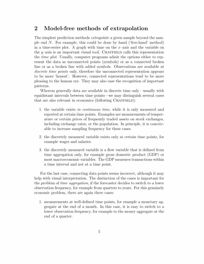
which yields least squares for β = 1. For β = 1− α, SES is obtained.Example. Figure 1 shows the application of SES to a time series of

Austrian private consumption. This version of exponential smoothing usesthe average over the first half of the sample as starting value x1.

7

1980 1985 1990 1995 2000 2005 2010

−0.02

0.00

0.02

0.04

0.06

Figure 1: Growth rates of Austrian private consumption 1977–2011 at con-stant prices and single exponential smoothing. Solid curve is the data, shortdashes are SES values at α = 0.1, long dashes are SES values at α = 0.3.

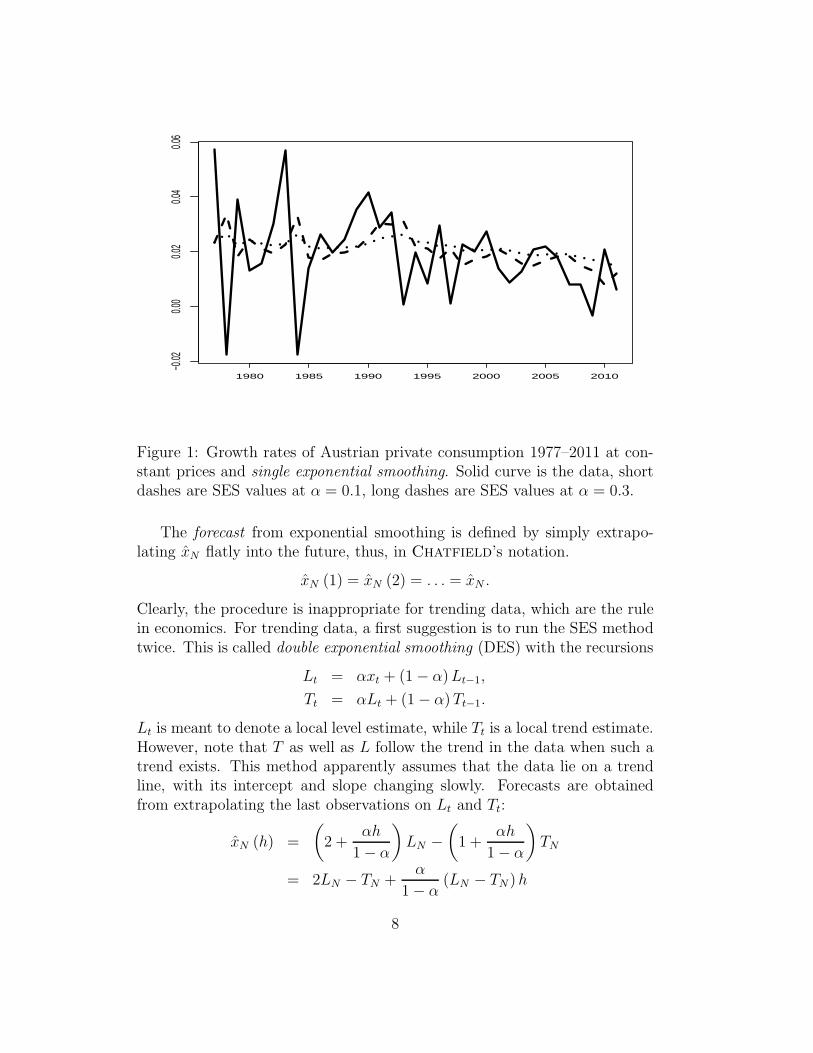
The forecast from exponential smoothing is defined by simply extrapo-lating xN flatly into the future, thus, in Chatfield’s notation.

xN (1) = xN (2) = . . . = xN .

Clearly, the procedure is inappropriate for trending data, which are the rulein economics. For trending data, a first suggestion is to run the SES methodtwice. This is called double exponential smoothing (DES) with the recursions

Lt = αxt + (1− α)Lt−1,

Tt = αLt + (1− α)Tt−1.

Lt is meant to denote a local level estimate, while Tt is a local trend estimate.However, note that T as well as L follow the trend in the data when such atrend exists. This method apparently assumes that the data lie on a trendline, with its intercept and slope changing slowly. Forecasts are obtainedfrom extrapolating the last observations on Lt and Tt:

xN (h) =

(

2 +αh

1− α

)

LN −

(

1 +αh

1− α

)

TN

= 2LN − TN +α

1− α(LN − TN )h

8

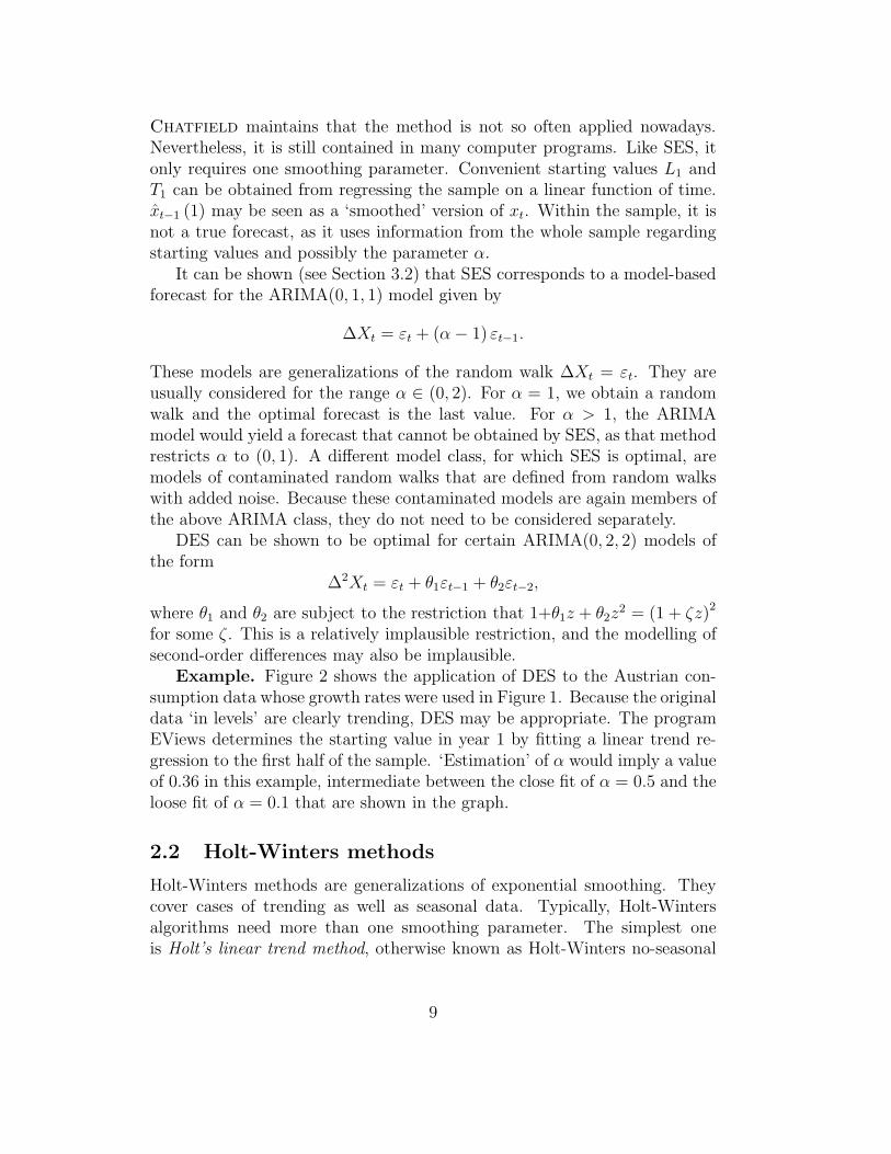
Chatfield maintains that the method is not so often applied nowadays.Nevertheless, it is still contained in many computer programs. Like SES, itonly requires one smoothing parameter. Convenient starting values L1 andT1 can be obtained from regressing the sample on a linear function of time.xt−1 (1) may be seen as a ‘smoothed’ version of xt. Within the sample, it isnot a true forecast, as it uses information from the whole sample regardingstarting values and possibly the parameter α.

It can be shown (see Section 3.2) that SES corresponds to a model-basedforecast for the ARIMA(0, 1, 1) model given by

∆Xt = εt + (α− 1) εt−1.

These models are generalizations of the random walk ∆Xt = εt. They areusually considered for the range α ∈ (0, 2). For α = 1, we obtain a randomwalk and the optimal forecast is the last value. For α > 1, the ARIMAmodel would yield a forecast that cannot be obtained by SES, as that methodrestricts α to (0, 1). A different model class, for which SES is optimal, aremodels of contaminated random walks that are defined from random walkswith added noise. Because these contaminated models are again members ofthe above ARIMA class, they do not need to be considered separately.

DES can be shown to be optimal for certain ARIMA(0, 2, 2) models ofthe form

∆2Xt = εt + θ1εt−1 + θ2εt−2,

where θ1 and θ2 are subject to the restriction that 1+θ1z + θ2z2 = (1 + ζz)2

for some ζ . This is a relatively implausible restriction, and the modelling ofsecond-order differences may also be implausible.

Example. Figure 2 shows the application of DES to the Austrian con-sumption data whose growth rates were used in Figure 1. Because the originaldata ‘in levels’ are clearly trending, DES may be appropriate. The programEViews determines the starting value in year 1 by fitting a linear trend re-gression to the first half of the sample. ‘Estimation’ of α would imply a valueof 0.36 in this example, intermediate between the close fit of α = 0.5 and theloose fit of α = 0.1 that are shown in the graph.

2.2 Holt-Winters methods

Holt-Winters methods are generalizations of exponential smoothing. Theycover cases of trending as well as seasonal data. Typically, Holt-Wintersalgorithms need more than one smoothing parameter. The simplest oneis Holt’s linear trend method, otherwise known as Holt-Winters no-seasonal

9

1975 1980 1985 1990 1995 2000 2005 2010

7080

9010

011

012

013

014

0

Figure 2: Austrian private consumption 1976–2011 and double exponentialsmoothing (DES). Solid curve marks data, short dashes DES values at α =0.1 and long dashes DES values at α = 0.5.

method. Holt’s method defines a local trend Tt as well as a local level Lt bythe following recursions

Lt = αxt + (1− α) (Lt−1 + Tt−1) ,

Tt = γ (Lt − Lt−1) + (1− γ)Tt−1.

The local level is a weighted average of the observation and the value ‘pre-dicted’ from the last level and trend estimates. The local trend or slope is aweighted average of the increase in the local level and the last slope. Conve-nient starting values may be L1 = x1 and T1 determined as the sample meanof the first differences of the data. Note that the meaning of Tt differs fromthe DES method.

Holt’s procedure defines forecasts by

xN (h) = LN + hTN ,

such that xt−1 (1) = Lt−1 + Tt−1 can be viewed as a smoothed version of xt.While the procedure is motivated by being appropriate for data with slowlychanging local linear trends, it can be shown that it is optimal for certain

10

ARIMA(0, 2, 2) models, that is, for models such as

∆2Xt = εt + θ1εt−1 + θ2εt−2.

If a time series follows this model, it becomes only stationary after takingsecond-order differences. In economics, this second-order integratedness wasonly found for some price series and monetary aggregates. Nevertheless, ifmerely seen as a forecasting procedure, Holt’s linear trend method appearsto give good forecasts for many economic series.

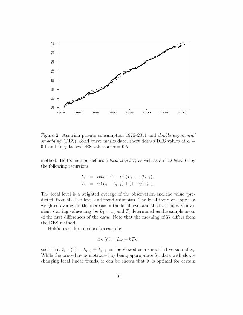
Example. Figure 3 shows the application of the Holt method to theAustrian consumption data. For larger α and small γ, we obtain a reasonablefit, while a loosely fitting curve trend is implied by large γ. The curves wereobtained by EViews, which uses true data values as starting values for thefirst time point here. This explains the deteriorating fit, as time progresses.

1975 1980 1985 1990 1995 2000 2005 2010

7080

9010

011

012

013

014

0

Figure 3: Austrian private consumption and Holt’s linear trend method. Solidcurve shows data, short dashes mark Holt values for α = 0.5 and γ = 0.1,while long dashes mark Holt values for α = 0.1 and γ = 0.9.

Gardner&McKenzie suggested to replace the forecast from Holt’smethod by a discounted forecast

xN (h) = LN +

(

h∑

j=1

φj

)

TN .

11

That forecast would be optimal for an ARIMA(1, 1, 2) model of the form

∆Xt = φ∆Xt−1 + εt + θ1εt−1 + θ2εt−2.

This model describes a variable that becomes stationary after first-orderdifferencing, which may be more plausible for most economic series. Thismay motivate its use in economic forecasting. However, it is less often foundin commercial computer software.

The true strength of the Holt-Winters procedure is that it allows for twovariants of seasonal cycles. This is important for the prediction of quarterlyand monthly economic series, which usually have strong seasonal variation.In the multiplicative version, level Lt, trend Tt, and seasonal St obey therecursions

Lt = αxtSt−s

+ (1− α) (Lt−1 + Tt−1) ,

Tt = β (Lt − Lt−1) + (1− β)Tt−1,

St = γxtLt

+ (1− γ)St−s,

where s is the period of the seasonal cycle, i.e. s = 4 for quarterly and s = 12for monthly observations. The algorithm needs three parameters α, β, γ.Forecasts are generated according to

xN (k) = (LN + TNk)SN+k−s,

where SN+k−s is replaced by the last available corresponding seasonal if k > s.In the additive version, the recursions change to

Lt = α (xt − St−s) + (1− α) (Lt−1 + Tt−1) ,

Tt = β (Lt − Lt−1) + (1− β)Tt−1,

St = γ (xt − Lt) + (1− γ)St−s.

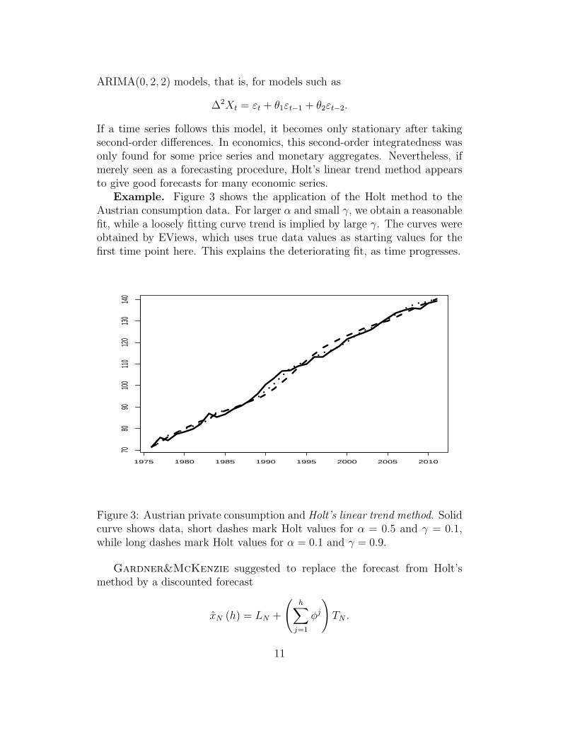
Example. Figure 4 demonstrates the application of Holt-Winters filter-ing to the quarterly Austrian gross domestic product (GDP). In this clearlyseasonal and trending series, both the multiplicative and the additive ver-sions yield similar performance. None of them can, of course, predict theglobal recession of 2008.

The time-series program ITSM includes an additive version of the sea-sonal Holt-Winters algorithm with automatically determined smoothing pa-rameters. For the Austrian GDP data, the algorithm determines α = 0.66,β = 0.05, γ = 1.00. The value of γ implies that the algorithm does not finda separate seasonal component in the data and extrapolates any of the fourquarters, simply based on the trend and noise components.

12

1990 1995 2000 2005 2010

4000

050

000

6000

070

000

Figure 4: Austrian gross domestic product 1988–2012 and Holt-Winters sea-sonal filtering. Forecasts from 2008.

2.3 Brockwell & Davis’ small-trends method

Among the many other ad hoc methods that have been suggested in theliterature, the small-trends method by Brockwell&Davis deserves to bementioned. It has been designed for variables with a ‘not too large’ trendcomponent and a seasonal component.

B&D assume that the trend is not too strong, therefore they concludethat the average of observations over one year yields a crude indicator of thetrend for that year. That ‘trend’, which is constant for any particular year,can be subtracted from the original observations. From the thus adjusted‘non-trending’ series, averages for one particular period (month k or quarterk) are calculated from the whole sample. For example, a January componentis calculated over all de-trended January observations. The resulting seasonalcycle and trend are then extrapolated into the future.

While there are obvious drawbacks of this method—the seasonal cycleis time-constant, no attempt is made at modelling the possibly stationaryremainder component nor the trend itself—the method has proved to be quitereliable for short time series. In their original contribution, B&D mentiona data set on monthly observations of road accidents for a time range ofa decade. Ten observations are not enough to permit sensible time-series

13

modelling.Example. An application of the small-trends method to the Austrian

GDP series is shown in Figure 5. At the end of the sample, 16 observationswere forecast from an extrapolation of the seasonal and trend components. Asexpected, the downturn of the global recession cannot be predicted perfectly.

1990 1995 2000 2005 2010

10.6

10.7

10.8

10.9

11.0

11.1

11.2

Figure 5: Austrian gross domestic product (solid curve), smoothed series,and four years of predictions from 2009 based on the small-trends method ofBrockwell&Davis.

14

3 Univariate time-series models

Forecasts based on time-series models require some tentative specificationof a statistical model that is conceivable as a data-generating process. Atleast for forecasting, it is not required that one believes that the used time-series model actually did generate the observations. Note that, particularlyin the tradition of Box&Jenkins, models are used when they are good anddiscarded when they are bad. The quotation from G.E.P. Box

All models are wrong but some are useful.

has become famous. It is obvious from the examples in the Box&Jenkins

book that some of the suggested time-series models are unlikely to have gen-erated the data. For example, Box&Jenkins use a second-order integratedARIMA model for an airline passenger series. It is hard to imagine the im-plied quadratic time trend to persist in the future development of airline traf-fic, even in the most optimistic outlook for an airline carrier. Box&Jenkins

stick to a philosophy of fitting models to observed data, as guided by somevisual inspection of time plots, correlograms, and other similar means, withthe purpose of short-term out-of-sample prediction. It is useful to review thebasic time-series models that are available as candidates for modelling in thefollowing subsections.

Prediction based on most of these models proceeds in an almost identicalfashion. Most models have the general form

Xt = g (Xt−1, Xt−2, . . . ; θ) + εt,

where g (.) is a (non-linear or linear) function that depends on an unknownparameter θ and εt is unpredictable from the past of Xt. The most rigor-ous assumption would be that εt is i.i.d., i.e. independent and identicallydistributed. Particularly in forecasting, the more liberal assumption of amartingale difference sequence (MDS) generally suffices for models of theabove type. A process (εt) is said to follow a MDS if and only if

E(εt|It−1) = 0,

where It−1 denotes some information set containing the process past. Ad-ditionally, it may be convenient to assume existence of some moments, forexample a variance should at least exist. In any case, the MDS assumptionis stronger than the backdrop assumption of linear time-series analysis, thewhite noise, defined by εt being uncorrelated over time. The white-noiseassumption does not preclude predictability using nonlinear models, whichwould invalidate some of the arguments in forecasting.

15

After specifying a time-series model (class), amodel selection stage followsin order to determine discrete specification parameters, such as lag orders.The selected model is estimated on the basis of a maximum-likelihood proce-dure or some convenient approximation thereof. The estimated parametersθ are inserted in place of the true ones θ and the approximate conditionalexpectation

g(

Xt−1, Xt−2, . . . ; θ)

≈ g (Xt−1, Xt−2, . . . ; θ) = E (Xt|Xt−1, Xt−2, . . .)

serves to determine Xt−1 (1). The same mechanism can be extended to obtain

multi-step predictions. For example, g(

Xt−1 (1) , Xt−1, . . . ; θ)

yields a two-

step forecast.Only in those cases where the design of the generating law is more com-

plex, such asXt = g (Xt−1, Xt−2, . . . ; εt; θ)

with genuinely non-linear dependence on the noise term, conditional expec-tation differs from g (Xt−1, Xt−2, . . . ; 0; θ) and it may pay to use stochas-tic prediction. For stochastic prediction, a statistical distribution is as-sumed for εt, and a large quantity of replications of the right-hand side

g(

Xt−1, Xt−2, . . . ; εt; θ)

are generated. The average of the replications then

approximates the conditional expectation. As an alternative to generatingεt from a parametric class of distributions, one may also draw εt replicationsfrom estimation residuals (‘bootstrapping’).

In nonlinear models of the latter type, εt should be independent over timeand have some time-constant moments. The more liberal MDS assumptionis less natural for these general models.

3.1 Linear models with rational lag functions

Most applications of time-series modelling use linear models. There are threebasic types of linear models: autoregressive (AR), moving-average (MA),and ARMA models. One view on these models is that they provide goodfirst-order approximations to the dynamics of the data-generating process.Another view is that they only intend to capture the first two moments ofthat DGP, i.e. means and covariances (including variance and correlations).Because all features are described exhaustively by the first two moments ina world of Gaussian distributions, the linear models are perfect for data thatare nearly Gaussian or for samples that are too small that there would beevidence to the contrary. To the forecaster, these simple linear models are at-tractive as long as non-Gaussian or non-linear features are not strong enough

16

that they can be successfully exploited by different models. Even for manydata sets that are known to contain non-linear dynamics, the non-linearityis either not time-constant enough or not significant enough to permit im-proved prediction. This justifies the popularity of these simple linear models,as they were suggested by Box&Jenkins.

3.1.1 Autoregressive (AR) models

AR models are the most popular time-series models, as they can be fullyestimated and tested within the framework of least-squares regression. Aseries Xt is said to follow an AR model if

Xt = φ1Xt−1 + φ2Xt−2 + . . .+ φpXt−p + εt.

This is the AR(p) model or the autoregressive model of order p. The errorεt is usually specified as white noise, i.e. as uncorrelated over time with aconstant variance and mean zero. Sometimes, time independence is alsorequired. Time-series statisticians often prefer a notation such as Zt for thewhite-noise error instead of εt. It is convenient to write the model in lagoperators, defined as BXt = Xt−1, as

Xt = φ1BXt + φ2B2Xt + . . .+ φpB

pXt + εt,

(1− φ1B − φ2B2 − . . .− φpB

p)Xt = εt,

φ (B)Xt = εt.

Some authors use L (lag) instead of B (backshift), without any change inthe meaning. The advantage of φ (B) lies in the isomorphism of lag polyno-mials and complex real-coefficients polynomials φ (z), with regard to manyproperties. For example, stability of the autoregressive model can be checkedeasily by calculating the roots (zeros) of φ (z). If all zeros of φ (z) are largerthan one in absolute value, there is a stationary process Xt, which satisfiesthe autoregressive equation and can be represented as

Xt =

∞∑

j=0

ψjεt−j.

The coefficients ψj converge to zero, such that∑

∞

j=0 |ψj | < ∞. Note thatψ0 = 1. If some roots are less than one, there may be a stationary ‘solution’,but it is anticipative, i.e. Xt depends on future εt. Such a solution is notinteresting for practical purposes. If some roots are exactly one in theirmodulus, no stationary solution exists. A typical case is the random walk

Xt = Xt−1 + εt,

(1−B)Xt = εt.

17

There is no stationary process that satisfies this equation.The coefficient series ψj is a complicated function of the p coefficients φj.

For the simple AR(1) model, it is easy to determine ψj , as

Xt = φXt−1 + εt

is immediately transformed into

Xt =

∞∑

j=0

φjεt−j.

The AR(1) model admits a stationary solution—is ‘stable’—whenever |φ| <1. For higher-order models, stability conditions on coefficients become in-creasingly complex. There is no way around an evaluation of the polynomialroots.

Stationary autoregressive processes have an autocorrelation function (ACF)ρj = corr (Xt, Xt−j) that converges to zero at a geometric rate as j → ∞.For the AR(1) process, ρj = φj is very simple. Higher-order AR processeshave cyclical fluctuations and other features in their ACF, before they finallypeter out for large j. One hopes that the sample ACF (the correlogram) re-flects this geometric ‘decay’, although it is of course subject to small-sampleaberrations.

Another characteristic feature of AR(p) models is that the partial auto-correlation function defined as

PACF (j) = corr (Xt, Xt−j |Xt−1, . . . , Xt−j+1)

becomes exactly zero for values larger than p. Time-series analysts say thatthe PACF ‘cuts off’ or ‘breaks off’ at p. Again, the sample PACF (or partialcorrelogram) may reflect this feature by becoming ‘insignificant’ after p.

Prediction on the basis of an AR(p) model is easy, as one simply replacesthe true coefficients by in-sample estimates φj and thus obtains one-stepforecasts immediately by

Xt−1 (1) = φ1Xt−1 + φ2Xt−2 + . . .+ φpXt−p.

Similarly, the next forecast at two steps is obtained by replacing the unknownobservation Xt by its prediction Xt−1 (1)

Xt−1 (2) = φ1Xt−1 (1) + φ2Xt−1 + . . .+ φpXt−p+1.

This algorithm can be continued to longer horizons. In that case, predictionswill converge eventually to the long-run mean. In these simple specifications,

18

the long-run mean must be zero. However, AR models are often specifiedwith a constant term

Xt = µ+ φ1Xt−1 + . . .+ φpXt−p + εt,

in which case the mean will be

EXt =µ

1− φ1 − . . .− φp

=µ

φ (1).

Note that the case φ (1) ≤ 0 has been excluded.

3.1.2 Moving-average (MA) models

A series Xt is said to follow a moving-average process of order q or MA(q)process if

Xt = εt + θ1εt−1 + θ2εt−2 + . . .+ θqεt−q,

where εt is again white noise. MA(q) models immediately define stationaryprocesses, every MA process of finite order is stationary. In order to preservea unique representation, usually the requirement is imposed that all zerosof θ (z) = 1 + θ1z + . . . + θqz

q are equal or larger than one in modulus.In that case, the MA model corresponds to the Wold representation ofthe stationary process. Wold’s Theorem tells that every stationary processcan be decomposed into a deterministic part and a purely stochastic part,with the stochastic part being an infinite-order MA process. The errors (orinnovations) of the Wold representation are defined as prediction errors, ifXt is predicted linearly from its past. This theorem motivates the generalusage of MA models in linear time series.

If all zeros of θ (z) are larger than one in modulus, the MA process hasan autoregressive representation of generally infinite order

∑

∞

j=0 ψjXt−j = εtwith

∑

|ψj | <∞. This excludes stationary MA processes with unit roots inθ (z). Thus, MA models are, as it were, more general than AR models. MAprocesses with an infinite-order autoregressive representation are said to beinvertible.

A characteristic feature of MA processes is that their ACF ρ (j) becomeszero after j = q. In fact, it is fairly easy to calculate all values of ρ (j) fromgiven MA coefficients θj . The property of the ACF should be reflected inthe correlogram, which should ‘cut off’ after q. By contrast, the partial ACFconverges to zero geometrically.

Forecasting from an MA model requires estimating the coefficients θj fromthe sample, after identification of the lag order q. While Box&Jenkins

suggested using visual inspection of correlograms for identifying q, most re-searchers nowadays use information criteria for this purpose. Estimates θj are

19

obtained from maximizing the likelihood or from some approximating com-puter algorithm. Additionally, estimates of the errors εt must be obtained,again using some computer algorithm. If θj and εs, s < t are available, aone-step forecast is calculated as

Xt−1 (1) = θ1εt−1 + θ2εt−2 + . . .+ θq εt−q.

More generally, j–step forecasts obey

Xt (j) =

q∑

k=j

θkεt+j−k

for j ≤ q, while forecasts will become trivially zero for j > q steps.

3.1.3 Autoregressive moving-average (ARMA) models

A series Xt is said to follow an autoregressive moving-average process of order(p, q) or ARMA(p, q) process if

Xt = φ1Xt−1 + . . .+ φpXt−p + εt + θ1εt−1 + . . .+ θqεt−q,

with εt white noise. The ARMA model is stable if all zeros of φ (z) arelarger than one. The representation is unique if all zeros of θ (z) are largeror equal to one in modulus and if φ (z) and θ (z) do not have common zeros.The stable ARMA model always has an infinite-order MA representation.If all zeros of θ (z) are larger than one, it also has an infinite-order ARrepresentation.

In practice, ARMA models often permit to represent an observed timeseries with a lesser number of parameters than AR or MA models. A repre-sentation with the minimum number of free parameters is often called par-simonious. Particularly for forecasting, parsimonious models are attractive,as the sampling variation in parameter estimates may adversely affect pre-diction. In small samples, under-specified ARMA models—i.e., with someparameters set to zero, while they are indeed different from zero—often givebetter predictions than correctly specified ones.

For ARMA processes, both ACF and partial ACF approach zero at a ge-ometric rate. It is difficult to determine lag orders p and q for ARMA modelsfrom visual inspection of correlograms and partial correlograms. While someauthors did suggest extensions of the correlogram (extended ACF, extendedsample ACF ), most researchers determine lag order by comparing a set oftentatively estimated models via information criteria.

20

After estimating coefficients θj and φj by some approximation to maxi-mum likelihood and calculating approximate errors εs, s < t, one-step fore-casts are defined by

Xt−1 (1) = φ1Xt−1 + . . .+ φpXt−p + θ1εt−1 + θ2εt−2 + . . .+ θq εt−q.

Two-step forecasts are obtained from

Xt−1 (2) = φ1Xt−1 (1) + φ2Xt−1 + . . .+ φpXt−p+1 + θ2εt−1 + . . .+ θq εt−q+1.

3.2 Integrated models

In many data sets, stationarity appears to be violated, either because ofgrowth trends, regular cyclical fluctuations, volatility changes, or level shifts.In all these cases, expectation and/or variance appear to be changing throughtime. However, signs of non-stationarity do not necessarily justify discardingthe linear models. In order to ‘beat’ ARMA prediction, a model class hasto be found that can do better. In the absence of such a model class, itis advisable to work with the available ARMA structures. For the veryspecial cases of trending behavior and of seasonal cycles, integrated modelsare attractive. The idea of an integrated process is that the observed variablebecomes stationary ARMA after some preliminary transformations, such asfirst or seasonal differences.

In detail, a variable is said to be first-order integrated or I(1), if it isnot stationary while its first difference ∆Xt = Xt − Xt−1 is stationary andinvertible (i.e. excluding the case of unit roots in the MA part) ARMA. Itis said to be second-order integrated or I(2), if its second-order differences∆2Xt = ∆(Xt −Xt−1) = Xt − 2Xt−1 + Xt−2 are stationary and invertibleARMA. When the differences are ARMA(p, q), Box&Jenkins were usingthe notation ARIMA(p, 1, q). Again, the ‘I’ in ARIMA stands for ‘integrated’.

For the decision on whether to take first differences of the original vari-able, Box&Jenkins suggested visual analysis. The correlogram of a first-order integrated variable decays very slowly, while the correlogram of itsfirst difference replicates the familiar ARMA patterns. The correlogram ofsecond differences of an I(1) variable or of first differences of a stationaryARMA (or I(0)) variable is dominated by some strong negative correlationsand tends to be more complex again. Box&Jenkins called this the caseof ‘over-differencing’. Following the statistical test procedures developed byDickey&Fuller around 1980, most researchers opine that visual analysismay not be reliable enough. We note, however, that Box&Jenkins didnot target statistical decisions and true models. For forecasting, differenc-ing may imply an increase in precision, even when the original variable is

21

I(0) and not I(1). Motivated by robustness toward structural breaks andsimilar features, the benefits of ‘over-differencing’ were analyzed in detail byClements&Hendry (1999).

The test by Dickey&Fuller requires running the regression

∆Xt = µ+ τt+ φXt−1 + γ1∆Xt−1 + . . .+ γp∆Xt−p + εt.

Significance points for the t–statistic of the coefficient φ were tabulated byDickey&Fuller. The null hypothesis is I(1) or ‘taking first differences’. Ifthe t–statistic is less than the tabulated points, one may continue with theoriginal data. The number of included lags p is usually selected automaticallyaccording to information criteria. For data without a clearly recognizabletrend, the term τt is omitted. That version of the test requires slightlydifferent significance points. In order to test for second-order differencing,the test procedure can be repeated for ∆X instead of X , with ∆2X replacing∆X . This second-order test usually is conducted on the version without theterm τt.

Economic variables are often sampled at a quarterly frequency. Such vari-ables tend to show seasonal cycles that change over time yet have some per-sistent regularity. For example, construction investment may show a troughin the winter quarter, while consumption may peak in the quarter beforeChristmas. Then, the mean is not time-constant and the variables are notstationary. A traditional tactic is to remove seasonality by seasonal adjust-ment and to treat the adjusted series as an integrated or stationary process.Seasonal adjustment is performed by sophisticated filters that, unfortunately,tend to remove some dynamic information and to imply a deterioration inpredictive performance.

Box&Jenkins suggested the alternative strategy of seasonal differences.Later authors called a variable seasonally integrated if its seasonal differences∆4Xt = Xt−Xt−4 are stationary and invertible ARMA.WhileBox&Jenkins

based the decision on whether to apply seasonal differencing on a visualinspection of correlograms, Hylleberg et al. developed a statistical test,whose construction principle is similar to the Dickey-Fuller test. Notethat seasonal differencing removes seasonal cycles and the trend, such thatfurther differencing of ∆4Xt is usually not required on purely statisticalgrounds. By contrast, Box&Jenkins liberally conducted further differenc-ing, which again is possibly justified if one aims at good prediction modelsrather than at true models.

In detail, Box&Jenkins suggested SARIMA models (seasonal ARIMA)with the notation (P,D,Q) × (p, d, q), which is to mean that D times thefilter ∆4 and d times the filter ∆ is applied on the original series, while P

22

and Q stand for seasonal ARMA operators of the form Θ (B) = 1 +Θ1B4 +

Θ2B8 + . . . + ΘPΘ

4P etc. Instances are rare, where the SARIMA approachappears to be appropriate. No example is known where D > 1 could beapplied sensibly.

Additionally to ARMA modelling of seasonal differences, SARIMA mod-els, and seasonal adjustment, a monograph by Franses offers another alter-native. Franses considers periodic models that essentially have coefficientsthat change over the annual cycle, i.e. each quarter has different coefficients.Clearly, a drawback is these models require estimating four times as manyparameters, which implies that reliable modelling needs longer samples.

At this point, we can proof the ARIMA(0,1,1) equivalence of SES. If thegenerating process is

∆Xt = εt + (α− 1) εt−1,

conditional expectation yields the forecast

Xt(1) = Xt + (α− 1)εt,

assuming we know the error εt at time point t. In theory, this εt can beretrieved as the difference Xt− Xt−1(1), and substitution immediately yieldsthe recurrence equation for SES. In practice, α will not be known, and fore-casts will differ from true conditional expectations.�

3.3 Fractional models

Fractional or long-memory models are linear models outside of the ARMAframework. While it is easy to define ∆0 as the identity operator (i.e., nothingchanges) and ∆1 = ∆, it is less straightforward to define ∆d for 0 < d < 1.This can be done by expanding (1− z)d as a power series

(1− z)d = 1 + δ1z + δ2z2 + . . . (1)

It turns out that δj are given by binomial expressions. If the power seriesconverges, one may define

∆dXt = Xt + δ1Xt−1 + δ2Xt−2 + . . . (2)

Time-series models may assume that ∆d is the required operator that yieldsa white noise or a stationary ARMA variable. Then, Xt can be called I(d) inanalogy to the cases d = 0, 1, 2, . . . It can be shown that I(d) variables withd < 0.5 are stationary, while d ≥ 0.5 defines a non-stationary variable. Thesefractional models describe processes whose autocorrelation function decaysat a slower than geometric pace. They are sometimes used for variables with

23

some indication of ‘persistent’ behavior in conjunction with some signs ofmean reversion, such as interest rates or inflation.

A drawback of these models is that they need very long time series sam-ples for a reliable identification of d and of the ARMA coefficients of ∆dX .Therefore, they pose a particular challenge to the forecaster.

3.4 Non-linear time-series models

General non-linear time-series models have become popular through the bookby Tong. A more recent and very accessible introduction was provided byFranses&VanDijk. Fan & Yao and Terasvirta et al. are representa-tive for the current state of the art in this field. Because non-linear structuresrequire large data sets for their correct identification and for potential im-provements in forecasting accuracy, the literature focuses on applications infinance and in other sciences, where large data sets are available.

ARCH (autoregressive conditional heteroskedasticity) models are a spe-cial case. Introduced by Engle in 1982 for monthly inflation data, theirmain field of applications quickly moved to financial series, for which vari-ous modifications and extensions of the basic model were developed. Unlikeother non-linear time-series models, ARCH models have been rarely appliedoutside economics. Many researchers in finance apparently prefer stochasticvolatility (SV) models to ARCH, which however are difficult to estimate.

3.4.1 Threshold autoregressions

The general non-linear autoregressive model

Xt = f (Xt−1, Xt−2, . . . , Xt−p) + εt

for some non-linear function f (.) would require non-parametric identifica-tion of its dynamic characteristics. Often, the identified function will notconform to stability conditions, such that simulated versions of the modeltend to explode. A well-behaved and simple specification is the piecewiselinear threshold model

Xt = φ(j)Xt−1 + εt, rj−1 < Xt−1 < rj, j = 1, . . . , k,

where rk = ∞ and r0 = −∞. The literature has called this model the SETAR(self-exciting threshold autoregressive) model and has reserved the simplername TAR for cases where φ(j) may be determined from exogenous forcesrather than Xt−1. The model can be—and has been indeed—generalizedinto many directions, such as longer lags, moving-average terms etc. SETAR

24

can be shown to be stable for strict white noise εt and for∣

∣φ(j)

∣

∣ < 1 for allj. It is interesting that this is only a sufficient condition. SETAR modelscan be stable for ‘explosive’ coefficients

∣

∣φ(j)

∣

∣ > 1 in the central regions, i.e.j 6= 1, k. Economics applications include interest rates and exchange rates,which are series where thresholds can be given an interpretation.

Note that, while for given rj all coefficients can be simply estimated byleast squares, identification of k and of the rk thresholds is quite difficult. Ifsome ‘regimes’ are poorly populated in the sample, neither their exact bound-aries nor their coefficients can be estimated reliably. Therefore, instances ofsuccessful forecasting applications are rare.

3.4.2 Smooth transition

The rough and maybe implausible change in behavior at the threshold pointsin the SETAR model has motivated the interest in smoothing the edges.Franses&VanDijk give a simple example of a smooth-transition autore-gressive (STAR) model by

Xt = φ(1)Xt−1 (1−G (Xt−1; γ, c)) + φ(2)Xt−1G (Xt−1; γ, c) + εt,

where G (.) is a transition function whose shape is determined by the pa-rameters γ (‘smoothness’) and c (‘center’). The left limit of the transitionfunction should be 0 (for Xt−1 → −∞) and the right limit should be 1 (forXt−1 → ∞). Curiously, these transition functions—a typical choice is a lo-gistic function—resemble the squashing functions of neural networks. Thecorrect specification and identification of the functions is difficult. Like alltime-series models, applications usually include deterministic intercepts thatmay also change across regimes.

3.4.3 Random coefficients

Instinctively, many empirical researchers think that the model

Xt = φtXt−1 + εt

would be more general than a standard AR(1) and may respond to the needsof an ever-changing environment. Unfortunately, this model is void withoutspecifying the evolution of the coefficient series φt. Stable autoregressions(φt = ψφt−1 + ηt) and white noise have been suggested in the literature.Curiously, some variants have been shown to come close to ARCH models.If Eφt = 1, the model is sometimes said to contain a ‘stochastic unit root’.

25

3.4.4 ARCH models

Many financial time series, such as returns on common stocks, are nearly un-predictable. Neither ARMA models nor non-linear time-series models allowreliable and possibly profitable predictions. However, these series digress intwo aspects from usual white noise, as it would be generated from a Gaussianrandom number generator. Firstly, the unconditional distribution is severelyleptokurtic, with more unusually large and small realizations than would beimplied from the Gaussian law. Secondly, calm and volatile episodes are ob-served, such that at least the variance appears to be predictable. The ARCHmodel by Engle appears to match both features. A variable X is said tofollow an ARCH process if it obeys two equations, which are called the ‘meanequation’ and the variance or volatility equation. For example, consider thesimple ARCH(1) model

Xt = µ+ εt,

E(

ε2t |εt−1

)

= ht = α0 + α1ε2t−1.

The model is stable (asymptotically stationary) for α0 > 0 and α1 ∈ (0, 1).Later, it was found that it is actually also stable for some α1 ≥ 1, dependingon distributional assumptions. In these cases, the variable Xt has infinitevariance but it is strictly stationary. The model yields leptokurtic Xt and italso implies sizeable ‘volatility clustering’, meaning that ht is serially (pos-itively) correlated. In stationary ARCH processes with finite variance, themean and variance of Xt are time-constant. It is only the conditional vari-ance ht that is time-changing. If the mean equation is replaced by a stableARMA Φ(B)Xt = µ+Θ (B) εt, the generated variable Xt is ARMA. In thisrespect, the model is still ‘linear’. Some authors even considered specifyinga non-linear mean equation.

Today, the most popular variant of the ARCH model is the GARCH(1,1)model

Xt = µ+ εt,

E(

ε2t |εt−1

)

= ht = α0 + α1ε2t−1 + βht−1.

The model may be extended by including a non-trivial first equation, forexample an ARMA model. In the GARCH model, the dependence of htand ht−1 is modelled directly. Stationarity and finite variance are implied byα0 > 0, α1 + β ∈ (0, 1), α1 > 0, β ≥ 0. Again, larger coefficients may retainstationarity, though not finite variances.

Judging by statistical significance of coefficients, the GARCH model wasapplied successfully to all kinds of financial variables, such as stock returns,

26

exchange rates, or interest rates, when these are observed at a moderatelyhigh frequency, such as weekly or daily. Prediction of volatility based on themodels has been less successful. While most forecast evaluation criteria aretuned to mean prediction, it is doubtful whether prediction of X2

t is a goodmeasure for the predictive accuracy of volatility forecasts. Taylor suggestedvarious alternatives for this purpose, which have however not been taken upmuch in the literature. Clements (2005) provides a more recent review ofthis problem.

Many econometric computer programs now contain GARCH estimationroutines. A slightly inefficient iterative routine for the ARCH specificationwas suggested by Engle in his original contribution. He suggests estimatingboth the mean equation and the variance equation by weighted least squares,replacing the ε2t for the ht and determining the weights from the most recentiteration. Therefore, given a conveniently long sample, ARCH models caneven be estimated by ordinary least-squares routines.

3.5 Neural networks

Based on the reports of some surprising successes of forecasts, neural networkmodelling has become popular in the 1990s. To econometricians, a stumblingblock to the application of neural networks (NN) is the quaint language thatwas adopted by NN adherents. The book by Chatfield (section 3.4.4)allows an interesting insight into NN modelling and re-positions it amongthe other non-linear procedures.

The main difference to non-linear time-series modelling is the focus on un-observed variables, which serve as black-box connections between inputs andoutputs. Similar unobserved ‘layers’ are used in the unobserved-components(UC) models suggested by Harvey who calls them ‘structural’. Note thatunobserved variables also appear in ARCH models (ht). Input variables,hidden variables, and output variables are connected by linear and S–shaped‘squashing’ functions, the latter ones resembling those in the STAR mod-els. These squashing functions motivate the word ‘neural’, as nerve cells orneurons react to a stimulus in a similar S–shaped way. Model selection andparameter estimation can be performed on the first portion of the data, whichis then called the ‘training set’. NN adherents call the model selection stagethe choice of ‘architecture’. Alternatively, the model selection and fittingmay be done by optimizing the forecasting performance on a second part ofthe sample, the ‘testing set’. Implied parameter estimates are usually neithertabulated nor published. In this regard, NN modelling resembles Bayesiantime-series applications such as BVAR (Bayesian vector autoregression, dueto Doan&Litterman&Sims). The suggestion to revise the architecture

27

and parameter estimates, as new data come in, is not specific to NN. There-fore, NN models ‘learn’ as much as other time-series models.

Apparently, the reported benefits of NN modelling with respect to predic-tion are mainly due to their usage of non-linear squashing functions. Most NNapplications in economics use just one layer of hidden ‘nodes’. Chatfield

gives an example for the implied output reaction function of a single-layerNN, which here is simplified slightly to

xt = φ0

(

wc0 +

H∑

h=1

wh0φh

(

wch +

h∑

j=1

wjhxt−j

))

,

with φj, j = 0, . . . , h denoting functions and wjk denoting coefficient parame-ters. Autoregressive linear combinations of lagged x with different maximumorder cause a reaction by the unobserved hidden H ‘neurons’ that is de-scribed by the functions φh. A linear combination of the H neurons thencauses another, potentially non-linear, reaction φ0 in the systematic partof the x variable at time t. The ‘stochastic’ difference of xt and xt is notmodelled explicitly.

3.6 State-space modelling

Like ARMA modelling and neural networks, state-space modelling is a differ-ent approach to time-series analysis rather than a class of different models.Often, state-space modelling leads to time-series models that are equivalentto ARMA models. A basic idea is that the observed series are generated asa ‘contaminated version’ of an output from an unobserved black-box systemwith its own intrinsic dynamic behavior. In other words, dynamic modellingis shifted from the observed variable to one or more unobserved variables.

In Chatfield’s notation, an observation equation

Xt = h′tθt + nt

explains the observed X as a linear combination (the vector h′t) of unobservedstate variables θt plus a ‘noise’ error nt. The transition equation

θt = Gtθt−1 + wt

extrapolates the unobserved system variables from their past. Gt is a squarematrix that conforms to the dimension of the unobserved state, i.e. the num-ber of state variables. Another stochastic error wt is permitted. In thismost general form, the system is clearly not identifiable. Under certain re-strictions, estimates of h, θt, G etc. are obtained from an algorithm called

28

the Kalman filter. All ARMA models can be re-written in this form, withconstant G and h.

The most popular specification for a state-space model in economics is the‘structural’ unobserved-components model by Harvey. Its simplest variantis

Xt = µt + nt,

µt = µt−1 + βt−1 + w1,t,

βt = βt−1 + w2,t.

Note that the state is two-dimensional and has the variables µ and β. Whileβt is a random walk, µt is an I(2) process. Therefore, Xt is implicitly also as-sumed as an I(2) process. Because we know that very few economic variablesare likely to be I(2), the model is difficult to justify within the framework oflinear modelling. The argument of Harvey and his numerous followers isthat the variances and relative variances of the errors n and w1, w2 make themodel quite flexible in the sense that the variance of w2 simply approacheszero if Xt is really an I(1) variable. Indeed, note that for w2t = 0, Xt reducesto a random walk plus noise. On the other hand, it is not to be expected thatthe choice of three variance parameters allows an equally powerful modellingtool as p + q ARMA parameters would. The reported success of Harvey’smodels relies mainly on the fact that many economic series approximatelycorrespond to the given dynamic structure. Whenever the dynamics digressfrom the basic pattern, the models can have a very poor performance.

It is shown easily that the above model corresponds to a specific ARIMAstructure with d = 2, and that the ARMA coefficients are simple functions ofthe relative error variances. From these properties, it is quite clear that themodel is not a generalization of I(1) models that allow the average growthrate to be time-changing, as some authors apparently believe. An advantageof the ‘structural’ models is that they directly yield estimates of ‘local’ trendsµt and of ‘local’ growth rates βt. The local trends provide smoothed versionsof the original series that are sometimes interpreted as having economic con-tents. For example, a smoothed output series may be interpreted as potentialoutput.

There is specialized computer software for ‘structural’ modelling, whichalso allows for some additional complexities, such as seasonal cycles in thestate variables or even business cycles. It is also possible to allow for someautocorrelation in the noise terms and to estimate their intrinsic dynamicsby non-parametric methods. That approach highlights the conceptual differ-ence between ARMA and UC modelling. While ARMA modelling targets adescription of the dynamic behavior of the observed variables, UC modelling

29

focuses on a decomposition of the observed series into a systematic and anoise part. The implied models as well as the underlying dynamic behaviorof the observed variables can be the same in both approaches.

30

4 Multivariate forecasting methods

Usually, multivariate forecasting methods rely on models in the statisticalsense of the word, though there have been some attempts at generalizingextrapolation methods to the multivariate case. This does not necessarilyimply that these methods rely on models in the economic sense of the word.Rather, one may classify multivariate methods with regard to whether theyare atheoretical, such as time-series models, or structural and theory-based.Words can be confusing, however, as the so-called ‘structural time-seriesmethods’ suggested by Harvey are actually atheoretical and not theory-based. Truly structural forecasting models with an economic backgroundwill be left for the next unit.

4.1 Is multivariate better than univariate?

Multivariate methods are very important in economics and much less soin other applications of forecasting. In standard textbooks on time-seriesanalysis, multivariate extensions are given a marginal position only. Em-pirical examples outside economics are rare. Exceptions are data sets witha predator-prey background, such as the notorious data on the populationof the Canadian lynx and the snowshoe hare. By contrast, the multivariateview is central in economics, where single variables are traditionally viewed inthe context of relationships to other variables. Contrary to other disciplines,economists may even reject the idea of univariate time-series modelling ongrounds of the theoretical interdependence, which appears to be an exagger-ated position.

In forecasting, and even in economics, multivariate models are not neces-sarily better than univariate ones. While multivariate models are convenientin modelling interesting interdependencies and achieve a better (not worse)fit within a given sample, it is often found that univariate methods outper-form multivariate methods out of sample. Among others, one may name aspossible reasons:

1. Multivariate models have more parameters than univariate ones. Everyadditional parameter is an unknown quantity and has to be estimated.This estimation brings in an additional source of error due to samplingvariation.

2. The number of potential candidates for multivariate models exceeds itsunivariate counterpart. Model selection is therefore more complex andlengthier and more susceptible to errors, which then affect prediction.

31

3. It is difficult to generalize nonlinear procedures to the multivariatecase. Generally, multivariate models must have a simpler structurethan univariate ones, to overcome the additional complexity that isimposed by being multivariate. For example, while a researcher mayuse a nonlinear model for univariate data, she may refrain from usingthe multivariate counterpart or such a generalization may not havebeen developed. Then, multivariate models will miss the nonlinearitiesthat are handled properly by the univariate models.

4. Outliers can have a more serious effect on multivariate than on univari-ate forecasts. Moreover, it is easier to spot and control outliers in theunivariate context.

An additional complication is conditional forecasting, which means thata variable Y is predicted, while values for a different variable X are as-sumed over the prediction interval. If X is a policy variable, it may makesense to regard it as fixed and not to forecast it. Even then, true-life futureX may react to future values of Y , while that reaction is ignored in theconditional forecast. The arguments of ‘feedback’ by Chatfield and theso-called Lucas critique are closely related. Important contributions on thefeedback problem, with some relation to forecasting, are due to Granger

(Granger causality) and to Engle&Hendry&Richard (weak and strongexogeneity). If X is merely another variable that is also predicted over theprediction interval, though maybe using a simple univariate extrapolationmethod, these forecasts may be wrong and there will be another source oferror.

If the forecasting model is designed such that forecasts of one or morevariables of type X are not generated, while one or more variables of type Yare modelled as being dependent on X , the system is called open-loop. If allvariables are modelled as dependent on each other and on lags, the systemis called closed-loop. Even closed-loop systems may allow for deterministicterms, such as constants, trend, or other variables that can be assumed asknown without error at any future time point.

4.2 Static and dynamic forecasts

A clear distinction of in-sample model fitting and out-of-sample forecastingis even more important than for univariate models. If 1, . . . , T serves asthe time range for a ‘training set’, a model is selected on the basis of theseobservations, the model parameters are estimated from the very same set,and predictions are then generated for 2, . . . , T according to the generation

32

mechanism of the model, the ‘prediction errors’ will be mere residuals. Ifvariables are predicted over the time range T + 1, . . . , T + h without usingany further information on the ‘test set’, the differences between observations(if available) and predicted values will be true out-of-sample prediction errors.The exercise yields a sequence of a one-step, a two-step, ..., and an h–stepprediction, which are sometimes called a dynamic forecast. There are manyintermediate cases.

In static forecasts, true observations are used for all lagged values of vari-ables. This situation does not correspond to a forecaster who only usesinformation on the training set. Prediction errors from static forecasts aredifficult to classify. One would expect that they tend to increase from T + 1to T +h if the forecasting model misses an important part of the DGP, whichresults in the impression of a time-changing DGP. Otherwise, the errors canbe regarded as one-step out-of-sample prediction errors. If observations areused for explanatory current variables in regression-type prediction models,the resulting error comes closer to a residual. The expression ex-post predic-tion is used for both variants. Sometimes it is also used for mere in-samplefitting and calculating residuals.

Other intermediate cases are obtained if, for example, a model is selectedon the basis of the total sample 1, . . . , T +h, while parameters are estimatedfrom 1, . . . , T only. The resulting forecast is not really out-of-sample, and itsprediction error tends to under-estimate the true errors. Such exercises areoften presented in research work and are sometimes labelled incorrectly asout-of-sample prediction.

4.3 Cross correlations

An important exploratory tool for modelling multivariate time series is thecross correlation function (CCF). The CCF generalizes the ACF to the mul-tivariate case. Thus, its main purpose is to find linear dynamic relationshipsin time series data that have been generated from stationary processes.

In analogy to the univariate case, a multivariate process Xt is called(covariance) stationary if

1. EXt = µ, i.e. the mean is a time-constant n–vector;

2. E (Xt − µ) (Xt − µ)′ = Σ, i.e. the variance is a time-constant positivedefinite n× n–matrix Σ;

3. E (Xt − µ) (Xt+k − µ)′ = Γ (k), i.e. the covariances over time dependon the lag only, with non-symmetric n× n–matrices Γ (k).

33

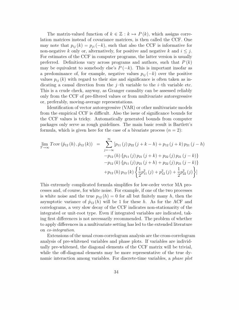
The matrix-valued function of k ∈ Z : k 7→ P (k), which assigns corre-lation matrices instead of covariance matrices, is then called the CCF. Onemay note that pij (k) = pji (−k), such that also the CCF is informative fornon-negative k only or, alternatively, for positive and negative k and i ≤ j.For estimates of the CCF in computer programs, the latter version is usuallypreferred. Definitions vary across programs and authors, such that P (k)may be equivalent to somebody else’s P (−k). This is important insofar asa predominance of, for example, negative values pij (−k) over the positivevalues pij (k) with regard to their size and significance is often taken as in-dicating a causal direction from the j–th variable to the i–th variable etc.This is a crude check, anyway, as Granger causality can be assessed reliablyonly from the CCF of pre-filtered values or from multivariate autoregressiveor, preferably, moving-average representations.

Identification of vector autoregressive (VAR) or other multivariate modelsfrom the empirical CCF is difficult. Also the issue of significance bounds forthe CCF values is tricky. Automatically generated bounds from computerpackages only serve as rough guidelines. The main basic result is Bartlett’sformula, which is given here for the case of a bivariate process (n = 2):

limT→∞

T cov (p12 (h) , p12 (k)) =∞∑

j=−∞

[p11 (j) p22 (j + k − h) + p12 (j + k) p21 (j − h)

−p12 (h) {p11 (j) p21 (j + k) + p22 (j) p21 (j − k)}

−p12 (k) {p11 (j) p21 (j + h) + p22 (j) p21 (j − k)}

+p12 (h) p12 (k)

{

1

2p211 (j) + p212 (j) +

1

2p222 (j)

}

]

This extremely complicated formula simplifies for low-order vector MA pro-cesses and, of course, for white noise. For example, if one of the two processesis white noise and the true p12 (h) = 0 for all but finitely many h, then theasymptotic variance of p12 (h) will be 1 for these h. As for the ACF andcorrelograms, a very slow decay of the CCF indicates non-stationarity of theintegrated or unit-root type. Even if integrated variables are indicated, tak-ing first differences is not necessarily recommended. The problem of whetherto apply differences in a multivariate setting has led to the extended literatureon co-integration.

Extensions of the usual cross-correlogram analysis are the cross-correlogramanalysis of pre-whitened variables and phase plots. If variables are individ-ually pre-whitened, the diagonal elements of the CCF matrix will be trivial,while the off-diagonal elements may be more representative of the true dy-namic interaction among variables. For discrete-time variables, a phase plot

34

refers to a scatter plot of a variable Xt and a lag, such as Xt−1 or Xt−j .If Xt has been generated by a first-order autoregression Xt = φXt−1 + εt,points should show a straight line with the slope corresponding to φ. Suchphase plots are particularly valuable if a nonlinear time-series relationship issuspected. With multiple time series, also phase plots of Xit versus Xj,t−k

can be considered, although the number of possible diagrams becomes largeand the variety of diagrams can become confusing.

4.4 Single-equation models

Two types of so-called single-equation models can be considered for multivari-ate forecasting: regression models and transfer-function models. Both typesare ‘open-loop’ models and model a dynamic relationship of an ‘endogenous’variable that depends on one or several ‘explanatory’ variables. The methodsare helpful in forecasting only if future values of the explanatory variablesare known, if forecasting of explanatory variables is particularly easy, or atleast if there is no dynamic feedback from the endogenous to the explanatoryvariables. In the latter case, the condition is similar to the requirement thatthere is no Granger causality running from the endogenous to the explanatoryvariables and that there is Granger causality from the explanatory to the en-dogenous variables. The concepts may not be entirely equivalent, as Grangercausality often only refers to linear relationships and additional conditionsmay be imposed by the parameterization of interest. These issues have beeninvestigated in the literature on exogeneity (Engle&Hendry&Richard).

The linear regression model can be assumed as known. In a time-seriessetting, errors are often correlated over time, such that ordinary least squares(OLS) may not be appropriate and some kind of generalized least squares(GLS) procedure should be considered. These GLS models assume two equa-tions, with a time-series model for the errors from the ‘means’ equation, forexample an ARMA model:

yt = β ′xt + ut

φ (B) ut = θ (B) εt.

The specification θ (B) = 1 and φ (B) = 1 − φB yields the classical GLSmodel that is used in the Cochrane-Orcutt or Prais-Winsten estimation pro-cedures. When these models are applied for forecasting, one does not onlyneed predicted values for x but also for u. Because ut is unobserved, it isusually replaced by in-sample residuals from the means equation and by out-of-sample predictions based on these residuals. The difference between trueerrors u and estimated residuals u brings in another source of uncertainty,

35

adding to the sampling variation in the coefficient estimates β, φ, and θ.In many cases, it is more advisable to replace the means equation by a dy-namic version that contains lagged values of yt and of some xt as furtherexplanatory variables, and whose errors are approximately white noise (dy-namic regression). An efficient search for the optimal dynamic specificationof such equations can be lengthy and may resemble the techniques used intransfer-function modelling. Thus, the two methods are not too different inspirit. It can be shown that static GLS models are a very restrictive version ofdynamic regression models. Some authors recommend removing trends andseasonals from all variables or possible differencing before regression mod-elling, which however may be problematic and may entail a deterioration ofpredictive accuracy.

Transfer-function models are based on dynamic relationships among mean-and possibly trend-corrected variables yt (output) and xt (input) of the form

δ (B) yt = ω (B)xt + θ (B) εt. (3)

Three different lag polynomials must be determined, which can be difficult.A common suggestion is to start from an ARMA or ARIMA model for theinput variable xt and to apply the identified ‘filter’ to both input and output.It is then much easier to determine the remaining polynomial. Of specialinterest is the case that ωj = 0 for j < d. This indicates that x affects ywith a delay and that, for any h–step forecast for yt with h ≤ d, forecastsfor the input xt are not required. In this case, x is also called a ‘leadingindicator’ for y. In analogy to the GLS regression model, efficient forecastingneeds predictions for the unobserved error series, which are constructed byextrapolating in-sample residuals.

4.5 Vector autoregressions and VARMA models

These models usually treat all n variables in a vector variable X as ‘endoge-nous’. For stationary multivariate processes, a convenient parameterizationis the vector ARMA (VARMA) model

Φ (B)Xt = Θ (B) εt (4)

with the multivariate white noise series εt, defined by E(

εtε′

t−k

)

= 0 if k 6=0. The model is stable if all roots of det (Φ (z)) = 0 are larger than onein absolute value. The model is invertible, i.e. X can be expressed as aconvergent infinite-order vector autoregression, if all roots of det (Θ (z)) = 0are also larger than one. Uniqueness requires the roots of det (Θ (z)) = 0 tobe larger or equal to one. Unfortunately, this condition is necessary but not

36

sufficient for a unique representation. This is one of the reasons why vectorARMA models are rarely used in practice.

For Θ (z) ≡ 1, one has the vector AR or VAR model

Φ (B)Xt = εt,

which is quite popular in economics. The simple VAR(1) model for thebivariate case n = 2 can be written as

Xt = ΦXt−1 + εt,

with the 2× 2–matrix

Φ =

[

φ11 φ12

φ21 φ22

]

.

Of special interest are cases such as φ12 = 0. Then, the first variable X1

does not depend on past values of the second variable, although it may becorrelated with it and it may depend on its own past via φ11. There is noGranger causality from X2 to X1. The model reduces to a transfer-functionmodel. X1 can be forecasted via the univariate model X1,t−1 (1) = φ11X1,t−1

and generally asX1,t−1 (h) = φh

11X1,t−1.

Building on this forecast, a forecast for X2 can be constructed from thesecond equation. Similar remarks apply to the reverse case φ21 = 0.

For the general VAR(1) case, h–step forecasts are obtained from

Xt−1 (h) = ΦhXt−1,

where Φ2 = ΦΦ, Φ3 = Φ2Φ etc. Similarly, forecasts from VAR(p) models canbe constructed in strict analogy to the univariate case. The forecasts requirecoefficient estimates and a lag order p, which are determined from the ‘train-ing’ sample ending in t−1. While cross correlograms may be helpful in findinga good lag order p, many researchers choose it by minimizing multivariateinformation criteria. Estimation can then be conducted by OLS, which canbe shown to be efficient in the absence of further coefficient restrictions.

VARX and VARMAX models are extensions of the VAR and VARMAframework, which allow for exogenous (‘X’) variables whose dynamics are notspecified or whose dynamics at least does not depend on the modelled ‘en-dogenous’ variables. For forecasting, the X variables require an extrapolationtechnique or assumptions on their future behavior.

37

4.6 Cointegration

Although VAR modelling traditionally assumes stationarity of all series, itis not generally recommended to difference non-stationary components indi-vidually, as such a step may destroy important dynamic information. Thecritical issue is cointegration. In short, when there is cointegration, cointe-grated models should be used for forecasting. When there is no cointegration,series with an integrated appearance should be differenced.

Cointegration is said to exist in a vector time series Xt when some ofthe components are individually first-order integrated (I(1)) while the re-maining components may be stationary, and there is a linear combination ofall components expressed by a vector β such that β ′X is stationary (I(0)).Cointegration is non-trivial when β has non-zero entries at the integratedcomponents. Apart from this CI(1,1) cointegration, which reduces integra-tion order from one to zero, higher-order cointegration can be defined but itspractical applicability is limited and examples for applications are rare. Notethat there are slightly different definitions of CI(1,1) cointegration in the lit-erature but that the above definition is the most convenient for multivariateVAR modelling.

The issues at stake can be best motivated by considering a VAR systemthat possibly contains some integrated and some stationary components

Φ (B)Xt = εt.

It is easily shown that such systems can always be transformed into an error-correction form

∆Xt = ΦXt−1 + Γ1∆Xt−1 + . . .+ Γp−1∆Xt−p+1 + εt, (5)

where the matrices Φ and Γ1, . . . ,Γp−1 are one-one functions of the autore-gressive coefficient matrices Φ1, . . . ,Φp. Note that the lag order of the poly-nomial Γ (z) = I−Γ1z− . . .−Γp−1z

p−1 is p−1, while the lag order of Φ (z) isp. The crucial matrix is Φ. If the rank of Φ is zero, there is no cointegrationand the system is best handled in differences. If the rank of Φ is n, the systemis stable and should be handled in the original form without differencing. Ifthe rank is between 1 and p−1, there is cointegration. In this case, the rankof Φ yields the number of linearly independent cointegrating vectors in thesystem. Empirically, the rank of Φ is determined by a sequence of tests withthe null hypothesis ‘rank Φ ≤ k’ and the alternative ‘rank Φ > k’. All detailsare found in Johansen’s monograph. This rank determination procedurehas been integrated into many econometric software packages, such as RATSand EViews.

38

Once the rank has been determined, estimation of (5) is conducted byreduced-rank regression, a technique that was developed by T.W. Ander-

son. Usually, this estimation procedure has been implemented in economet-ric software together with the rank-determination sequence. Then, estimatesΦ and Γ1, . . . , Γp−1 can be substituted for the true matrices and h–step fore-casts are retrieved easily.

Ignoring cointegration issues and naively differencing non-stationary com-ponents implicitly assumes the restriction Φ = 0. If the true Φ 6= 0, this doesnot only imply mis-specification due to an incorrect restriction but this mis-specification has particular consequences. The forecasts will not reflect theproperty that β ′X is stationary, in contrast with the sample. In economics,the usual interpretation is that ‘equilibrium conditions are ignored’. For ex-ample, consumption or investment may amount to a relatively constant shareof national income in the sample, while that share may rise or fall in theforecast interval. Forecasts may violate theory-based plausibility conditions.Using simulation and algebraic techniques, the consequences of cointegrationfor forecasting were analyzed by Clements&Hendry and in two influen-tial studies by Engle&Yoo and by Christoffersen&Diebold. WhileEngle&Yoo demonstrated that cointegration may only be important forprediction at longer horizons, such as h > 10, Christoffersen&Diebold

showed that such results depend on which variable is targeted in predic-tion. Accurate prediction of the original components may be a different taskfrom predicting stationary variables such as ∆X and β ′X . In some specifi-cations, cointegration may even be important for one-step prediction, while,in other specifications, even long-horizon predictions are best conducted onthe basis of the original ‘level’ VAR Φ (B)Xt = εt, while the differences VARΓ (B)∆Xt = εt will typically suffer from serious mis-specification. As a bot-tom line, it is recommended to use cointegration techniques and the impliedprediction models. When no cointegration is found, one should use VARs indifferences.

4.7 Multivariate state-space models

State-space models, such as Harvey’s ‘structural’ time-series models, canbe generalized to the multivariate case. Chatfield draws particular atten-tion to the SUTSE (seemingly unrelated time-series equations) model withcommon trends

Xt = Θµt + µ∗ + nt,

µt = µt−1 + wt.

39

In this model, the matrix Θ is assumed as rectangular n×r with r < n, suchthat the second equation updates an r–dimensional integrated process. Somerestrictions on µ∗ and Θ are needed to identify the model. It can be shownthat n−r cointegrating relationships are implied by this model. The random-walk process µt is viewed as the ‘common trend’ of the system, which yieldsone out of several similar though conflicting definitions of ‘common trends’.In strict analogy to the remarks on univariate state-space models, also thesemodels are not really generalizations of VAR or vector ARIMA models andthey do not really allow for time-varying structure. They are equivalent tocertain vector ARIMA models and merely use a different parameterization.

40

5 Forecasts using econometric models

Even today, the basic workhorse tool for forecasting in economics is the largestructural econometric model. These models are developed in specialized in-stitutions, government agencies, and banks. They often consist of hundredsof equations. It is interesting that econometric theory has not been focusingon these models for almost thirty years. Following the general failure of thesemacro-econometric models to cope with the economies of the 1970s followingthe OPEC crisis, theory has discarded them (see Fair, for a noteworthy ex-ception to the rule). This attitude was supported by several empirical studiesthat generally concluded that time-series models yield better forecasts thanstructural models. From the angle of economic as well as econometric theory,Sims recommended multivariate time-series modelling instead of structuralmodels. He explicitly refers to the many ‘incredible’ exclusion restrictionsof macro-econometric models, while he also concedes that ‘large-scale mod-els do perform useful forecasting ... functions’. Chatfield’s assertion that‘econometric models are often of limited value to forecasters’ sounds muchharsher and may miss the point, as many large-scale models are built withthe purpose of forecasting in mind. Recently, calibrated dynamic stochasticgeneral-equilibrium (DSGE) models with a strong basis in economic theorybut with sometimes only loose fit to data have been used widely in policyevaluation and long-range scenarios. The value of such models for short-runmacroeconomic forecasting is still unsettled.

5.1 The classical macro-econometric model

The classical approach to macro-econometric modelling consists of severalsteps. Model building is indeed guided by theory but the model specificationis not really determined by theory. I distinguish the following phases:

1. choosing the variables to be included in the model;

2. separating the variables into endogenous and exogenous variables;

3. sketching a priori causal relationships among the variables, in the styleof a flow chart;

4. specification of estimable equations;

5. estimation;

6. forecasting.

41

Step 1 is guided by the intended purpose of the model. A model for theAustrian economy may include various Austrian economic variables and alesser variety of foreign variables, together with possibly some non-economicvariables such as population or weather conditions. An important restrictionis the availability of data. For example, a quarterly model could includemacroeconomic sub-aggregates of consumer demand or capital formation,while several government expenditure categories are available on an annualbasis only. Mixing different periodicities is sometimes considered but manymodelers find this option inconvenient.

Step 2 is crucial. Philosophers of science have named the classificationof variables into endogenous and exogenous variables as a characteristic ofeconometric research (Cartwright). In many other sciences, an analogousclassification rests on firm a priori beliefs, while such beliefs are rare ineconomics. No generally accepted theory can tell whether saving causesinvestment or investment causes saving. Similarly, there is no accepted causalordering between the interest rate and real output. Deterministic variables,such as constants and time trends, are always exogenous. If the model isdesigned to represent the domestic sector of a small open economy, foreignvariables are also usually regarded as exogenous. This may change if a worldmodel is targeted. Typical foreign variables would be world demand andprice indexes for the world market, while export prices and even import pricesmay respond to the domestic price structure. Many macroeconomic modelsalso view fiscal variables as exogenous. This decision is often dictated byinstitutional reasons, such as the preference of a government institution whofunds the forecasting project and does not want to be seen as a reaction nodewithout a free will. One may, however, also choose that option to allow forconditional forecasting, i.e. scenarios that respond to alternative governmentpolicies. Some macroeconomic models choose an intermediate solution andkeep aggregate tax revenues as endogenous, while they impose exogenoustax rates and long-range conditions such as a tendency of the budget to bebalanced. Non-economic variables are usually modelled as exogenous.

Step 3 determines the internal structure of the model. Often, the largeamount of considered variables is broken down into blocks of variables, suchas real demand variables, price indexes, labor market variables etc. Influ-ences across these blocks or sectors may run in both directions, though suchrelationships may be restricted to very specific effects. For example, the la-bor market may respond to the price sector via a Phillips-curve only. Causalorderings among blocks or variables are often not meant to specify dynamiccausal orderings. Rather, they indicate which variables will appear on theright-hand side of regression equations for specific left-hand side variables.While the explanatory variables may be accepted as lags in further specifica-

42

tions, some model builders have a skeptical view on such time lags and mayregard them as weak spots of their models. The economic science finds itdifficult to specify dynamic interaction and has to justify it by arguments ofhabit persistence, adjustment costs, delivery lags etc. There is little infor-mation on the exact form of these features, hence coefficients that describedynamic interaction are difficult to interpret. On the other hand, dynamicrather than static relationships in equations help in forecasting as well as instabilizing the system. In the extreme case of an n–variable static model, a‘solution’ for a given time point is calculated by solving a system of n oftennonlinear equations. Forecasting will not be possible, unless assumptionsare made on extrapolating n− 1 of the variables at a different (future) timepoint. The other extreme is a VAR or VARX system, where all influences aredynamic. A forecast for future time points is calculated by simple insertionof the current observed values.

Step 4 consists in a cursory search for equation specifications. In mostmacro-econometric models, this search is conducted on a single-equation ba-sis, in spite of persistent theoretical criticism. The dependent variable isspecified, for example private consumption of durable goods, and variouscombinations of explanatory variables are tried as regressors. The specifica-tion search is guided by the set of possible influences that was specified in step3. Functional forms, such as linear or double-log specifications, are selectedaccording to statistical criteria or, less often, to theory arguments. Possiblenonlinear forms in some equations are among the advantages of econometricmodelling relative to linear VAR systems. Usually, the final specification isrequired to fulfil the following criteria:

1. regressors should be statistically significant;

2. coefficients should have an economically interpretable size and signwhenever such interpretation is possible;

3. influences that are deemed to be important for theoretical reasonsshould exist, which often implies ‘keeping’ insignificant regressors;

4. residuals should not show substantial autocorrelation;

5. if inserted into the whole model, the equation should not de-stabilizethe model. A solution should be possible in a ‘range’ of values aroundthe observed data and for a reasonable ‘range’ of possible residualswithout obtaining inadmissible values, such as negative unemploymentrates;

43

6. measures such as R2 should be conveniently large, the required valuesranging between 0.3 and 0.95;

7. more general statistical tests of mis-specification should not indicatesevere violations of assumptions.

In many cases, these different targets are in conflict with each other.Modelers decide on their preferences among targets on an ad-hoc basis. Itis no wonder that Pindyck&Rubinfeld call model building a ‘science andart’.

Step 5 demands for detailed comments. According to the classical model-building framework, as set out by the Cowles Commission, linear econometricmodels can be written in the form

Y Γ = XB + U.

Many econometric models are nonlinear but this form may even serve as abasis for estimating nonlinear structures. Y is a matrix of dimension T ×Gand contains the observations on the G ‘endogenous’ variables, while Γ is aG × G–matrix of estimable coefficients. X is a matrix of dimension T ×Kand contains the ‘exogenous’ variables, including lags of endogenous vari-ables. Due to their similar estimation properties, exogenous (including laggedones) and lagged endogenous variables are summarized as predetermined vari-ables. Note that the wording ‘predetermined’ does not refer to a forecastingapplication, as data on current exogenous variables are usually not availablebefore the data on endogenous variables. B is a K × G coefficient matrix,while U contains regression errors.

Clearly, the matrix Γ cannot be estimated without further restrictions.It contains information on simultaneous relationships among the endogenousvariables and represents the completely ‘static’ aspect of the model. Withoutrestrictions, the system contains G different equations that look all alike. Theextreme case Γ = I is called the reduced form of the system. In a certaincontext, systems with Γ = I are also called SUR models (seemingly unrelatedregressions), as the only connection among equations is by common regressorsand by possible correlation of errors, which two aspects may be ignored atfirst sight. Reduced-form systems can always be estimated by regressionmethods. They are convenient for forecasting but economists avoid them, asthey do not reflect interdependencies that were developed in economic theory.Another argument against their usage is that their parameters are difficultto interpret. This argument again reflects the ‘hybrid’ aims of econometricmodelling: even when the model is built exclusively for prediction, economistsrequire its interpretability in economic terms.

44

The conditions on Γ that have to be imposed in order to make the model‘identified’, i.e. to allow its sensible empirical estimation, are rather complex.Most applied econometric models fulfil these conditions anyway, due to theirtendency to include ‘many unbelievable restrictions’, as Sims has put it. Inthese systems with general Γ, regression estimation of single equations yieldsinconsistent parameter estimates. The literature recommends variants of in-strumental variables estimation procedures, such as two-stage least squares(2SLS), in order to overcome this deficiency of least squares in ‘simultaneoussystems’. In empirical model building, this advice is not always followed.Many large-scale econometric models are estimated by least squares meth-ods, while in other models 2SLS estimation is restricted to some sensitivesub-systems. An informal argument in favor of this practice is that the in-consistency of least squares plays a lesser role in larger models. This maynot be true in general.

Finally, step 6 consists in substituting estimates for the unknown param-eters and to predict the endogenous variables via

Yt (1) = Xt+1BΓ−1,

which poses difficulties ifXt+1 is not available. Unless X contains only laggedendogenous variables—this is a special case of VAR modelling—Xt+1 will notbe available and has to be guessed or extrapolated. Other forecasters avoidthis ‘zero-residual’ forecasting and prefer

Yt (1) = Xt+1BΓ−1 + Ut+1Γ−1,

where Ut+1 are so-called ‘add factors’ that are guessed and inserted by theforecaster. This may make sense when the model has an annual frequencyand the current year is to be forecasted. Although the endogenous variablesare not yet available, some information has spread on the current economicsituation, which may discourage the automatic usage of zero residuals. Inpractice, the calibration of add factors according to informal information isthe principal and most time-consuming task of economic model forecasters.The above formulae are too simplistic, as they are valid for linear models only.With nonlinear models, simple multiplication by the inverted Γ is replacedby a numerical solution of a high-dimensional system of nonlinear equations.In former times, this step required a large amount of computer time, whichwas a binding constraint to forecasters. Nowadays, computers have becomeso powerful that even high-dimensional systems can be solved within a fewseconds.

45

5.2 An example

A prototypical example for a macro-econometric model is the national incomemodel by Granger:

Ct = a1 + b1Yt + eCt,

It = a2 + c2Pt−1 + eIt,

Tt = d3GDPt + eTt,

Pt = a4 + b4Yt + f4It−1 + ePt,

GDPt = Ct + It +Gt,

Yt = GDPt − Tt.

The endogenous variables are: consumption C, investment I, taxes T , prof-its P , gross domestic product GDP , disposable income Y . Apparently, theoriginal Granger called Y the ‘national disposable income’ out of a misun-derstanding, thus excluding the government sector from the national econ-omy. Rather, Y appears to be a disposable income of the household andfirm sectors. The exogenous variables are: government expenditure on goodsand services G and the constant. There are four structural or behavioralequations with error terms and two identities. The economy is closed, whichis clear from the GDP definition. There are two simultaneous feedback cy-cles: C depends on Y , Y depends on GDP , and GDP depends on C; Tdepends on GDP , GDP depends on C, C depends on Y , and Y depends onT . Therefore, least-squares estimation will yield inconsistent estimates of allparameters (coefficients).

By substitution, for example GDP can be expressed by the predeterminedvariables

GDPt = A+Gt

H+ c2

Pt−1

H+ eGt,

where A = (a1 + a2) /H , H = 1−b1+b1d3, and eGt = (eCt + eIt − b1eTt) /H .Analogous substitution yields the reduced form of the system, which ex-presses all six endogenous variables by predetermined variables and errorterms. Note that the error structure of the reduced form necessarily has asingular covariance matrix. The equations of the reduced form can be es-timated consistently by least squares. Econometric textbooks consider theoption of retrieving estimates for the original ‘structural’ coefficients ‘back-ward’ from these reduced form estimates by algebraic operations and call itindirect least squares. This method is rarely used in practice.

In order to forecast GDPt+1, one may use

GDP t (1) = A +Gt+1

H+ c2

Pt

H,

46

which assumes that approximations to the reduced-form coefficients A, H−1,and c2/H are available in any case, either from least squares on the reducedform or from two-stage least squares on the structural model and simple‘forward’ algebraic operations. While Pt is available at t, Gt+1 is not. Eitherone inserts a ‘plausible value’ for Gt+1, for example from the government’sbudget plan, or one uses an additional time-series or econometric equation forpredicting G. The latter option ‘essentially completes the system by treatingG as if it were endogenous’ (Granger), i.e. by endogenizing governmentpolicy. Granger suggests ‘to use a model to forecast G and then to alterthis forecast subjectively if relevant extra information is available to theforecaster. The success or lack thereof of such adjustments clearly depends onthe quality of the information being utilized and the abilities of the forecasterwho tries to use it’.

47

6 The LIMA forecasting model of the Insti-

tute for Advanced Studies Vienna

[Note: as a tool for professional short-term forecasting, the LIMA model issubject to a never-ceasing process of updates and minor modifications. Mostdetails and parameter estimates in this section reflect the situation as of2009.]

The LIMA model has grown out of the LINK project that attempts tojoin worldwide economic forecasting models into a common framework. Be-cause many of the variables are only available at an annual frequency, theLIMA model also operates at this annual frequency. This can be troublesomefor short-run prediction, as unofficial provisional data on main accounts ag-gregates come in on a quarterly basis. Therefore, LIMA is rarely run in itsoriginal form with zero residuals, and ‘add factors’ play a key role.

The LIMA model is a traditional macro-econometric prediction modelwith an emphasis on the economy’s demand side. Thus, the model may becalled a ‘Keynesian’ model. It has 99 equations, which implies 99 endoge-nous variables. As in most macro-econometric models, most equations aremere identities. Only 19 equations are ‘behavioral’ and contain estimatedcoefficients. With 99 endogenous variables and 19 structural equations, theLIMA model is a comparatively small macro-econometric model.

LIMA’s model structure is updated frequently. Some equations may bereplaced by better ones, while others are being eliminated in a search tosimplify the overall structure and again others are being added in order tosatisfy the needs for a more refined modelling of a certain sector of theeconomy. In the recent decade, the need for disaggregated modelling inmany sectors has decreased on average. Accordingly, the ‘true dimension’of the model has shrunk from a maximum of more than 30 to 19. The‘full dimension’ was even larger, due to a very elaborate bookkeeping modelfor the Austrian public sector. Notwithstanding all modifications, the basicLIMA model structure still resembles its predecessors from the late 1970’s.

Parameter estimates are updated once a year, when the official provisionaldata for the previous year become available, which is usually in September.For example, in September 2007 all equations were re-estimated using datafrom 1976 to 2006. For many equations, estimation intervals ended in 2005if provisional data were earmarked as likely to be revised further. 1976 is theearliest year, for which national accounts data are available that correspondto the ESA standard. With some temporary exceptions, all equations areestimated by OLS. Indications of mis-specification due to autocorrelationare adjusted by dynamic modelling rather than by GLS–type corrections.

48

Thus, most behavioral equations are dynamic.The model’s center piece is the domestic demand sector. Demand aggre-

gates are modelled in real terms, i.e. at constant prices, and sum up to realgross domestic product (GDP). Additional equations are used to determineprices and deflators. By multiplying those deflators into the real aggregates,nominal variables and eventually nominal gross domestic product (GDP$)are calculated. Following the transition from Paasche indexes to chained in-dexes in national accounts, adding-up identities of real variables do not holdexactly any more. This problem is resolved using artificial residual entitiesthat are small on average and will be ignored in further discussion.

This adding-up to obtain GDP requires export and import variables. Thetreatment of exports and imports is asymmetric. Imports are fully endoge-nous and respond to demand categories, such as consumer durables andequipment investment. By contrast, exports are mainly exogenous. OlderLIMA versions considered modelling exports as depending on world demandbut, unfortunately, data on world demand become available with a consid-erable time lag only, which excludes its usage for the practical purpose offorecasting. For export and import prices, the approach is reversed. Importprices are exogenous, as it is assumed that Austrians have to accept the worldmarket’s price level, while export prices are endogenous.

Another component of GDP is public consumption. In the current ver-sion, public consumption is exogenous. In earlier versions, nominal publicconsumption was modelled as resulting from the sum of spending categoriesof general government. This practice was abandoned, as most governmentspending categories are exogenous and as the resulting price deflator of publicconsumption was often implausible or caused instabilities in model solution.In contrast to spending, several components of government revenues are mod-elled as endogenous variables, such as direct taxes or contributions to socialsecurity. From this government sector, balancing items such as the budgetdeficit can also be calculated.

The real and government sectors also interact with the labor market sec-tor, which yields variables such as employment, the labor force, and wages.Other variables, such as the working-age population, are exogenous.

The LIMA model does not include a financial sector. Financial variablesthat are influential for the goods market, such as exchange rates and interestrates, are supplied by specialists on the financial sector who use separatemodels.

49

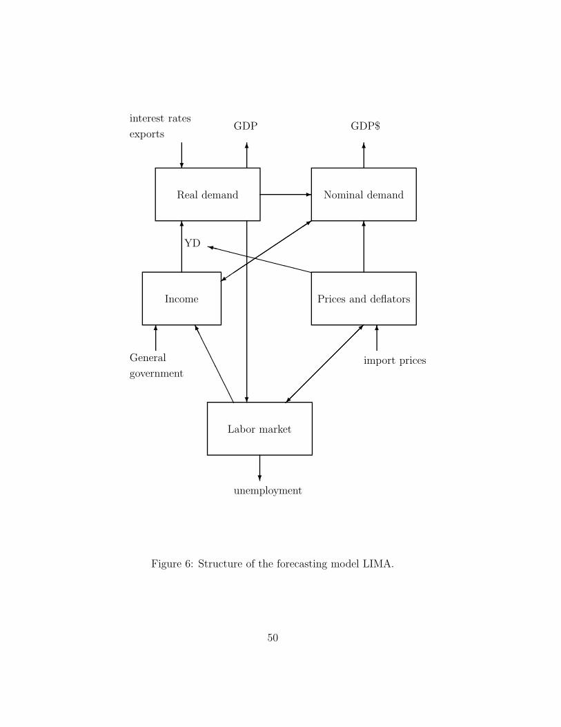
Real demand

interest rates

exportsGDP

?

6

6

?

Nominal demand

6

GDP$

-

Income

���������3��

��

��

��

��+

6

General

government

6

Prices and deflators

XXXXXXXXXXXXyYD

��

��

��

��������

�����

import prices

6

Labor market

AA

AA

AA

AAAK

unemployment?

Figure 6: Structure of the forecasting model LIMA.

50

6.1 A typical demand equation: private consumption

Consumer demand consists of three categories: consumer durables, consump-tion of other goods, and consumer services. Almost 50% of household expen-ditures are spent on services. The share of services in household consumptionappears to be increasing in the longer run. Before 1980, it used to be below45%. Until a few years ago, consumer demand equations could be speci-fied for the sub-aggregates, and total private consumption was obtained byadding the three forecasted categories. Unfortunately, updates of this de-composition are no more available with an acceptable time lag, and henceprivate consumer demand is now modelled on the basis of one behavioralequation only.

As a general rule, demand equations use logarithmic growth rates asdependent variables. Logarithmic growth rates are fairly constant in thelonger run, hence they come closer to fulfilling the assumption of stationaritythan, for example, first differences. On the other hand, percentage growthrates are far less convenient to handle from an econometric model builder’sviewpoint.

In consumer demand, the principal explanatory variable is the growthrate of household disposable income yd. The real variable yd is obtained fromdeflating nominal household income by the consumption deflator. Thus, thesame price index deflates income and the dependent variable.

Another potential source of explanation are error-correction relationshipsbased on the ‘great’ consumption-output ratio. A cointegrating regression oflog private consumption on log income

ct = b0 + b1ydt + ut

yields b1 = 1.067, slightly above one. One may argue, anyway, that unitelasticity for consumption should be imposed on the model, as otherwiselonger-run forecasts may yield over-consumption and ever-decreasing savingrates. Therefore, the theory-based long-run restriction b1 = 1 is used infurther modelling.

The estimation results (see Table 1) are acceptable. The estimation timerange has been shortened at its beginning, in order to exclude some outliersthat were caused by changes in the VAT tax rate. Maybe excepting laggedincome growth, all regressors are significant, and the (here, not very reliable)Durbin-Watson statistic does not indicate any serious specification error.The R2 is lower than in comparable consumption equations for other data,which would be an incentive to search for further explanatory variables. Ob-vious suggestions, such as interest rates at any lags or lags of the dependentvariable, failed to achieve significance. Several other variables were tried, for

51

example budget-consolidation indicators motivated by a Ricardian argumentor unemployment indicators that may set saving incentives due to house-holds’ fears of getting unemployed. Again, none of these indicators achievedsignificance.

Apart from a local dummy for the exceptional year 1983, the equationshows a ‘Keyenesian’ short-run reaction with an elasticity of around 0.8 toreal income, which is mitigated by a lesser contrary effect in the year af-terwards. The error-correction term has the correct sign and has convincingsignificance. Austrian households tune their consumption patterns to longer-run saving plans and correct past under- or over-consumption.

Table 1: Behavioral equation for private consumption. Estimation time rangeis 1979–2006. Dependent variable is log(ct/ct−1).

regressor coefficient t–valueconstant 1.337 3.721dummy83 0.042 4.924log(ct−1)− log(ydt−1) -0.298 -3.712∆ log(ydt) 0.802 6.734∆ log(ydt−1) -0.205 -1.666

R2 = 0.809, DW=1.710

6.2 Equipment investment

Besides consumption, investment or ‘gross fixed capital formation’ is anotherimportant component of aggregate demand. While the ESA system disag-gregates investment into a larger number of subcomponents, LIMA only con-siders equipment investment, which includes machinery and transportationequipment, and construction investment, which includes business as well asresidential construction. Equipment investment is the slightly smaller partbut its equation is more important than the construction investment coun-terpart, as construction often relies much on public funding and policy.

Until fairly recently, modelling of investment demand relied on a theory-based factor-demand framework and on a CES or Cobb-Douglas productionfunction. It was found, however, that dynamic error-correction modellingentailed better in-sample fit and also more stable out-of-sample predictiveperformance.

52

A cointegrating regression of logged equipment investment on gross do-mestic product (GDP) yields the form

log(ifet) = −4.09 + 1.323 log (yt) + ect,

where ife denotes equipment investment and y simply denotes GDP. Thelarge value of the elasticity coefficient may sound a warning, as it appearsto imply an ever-increasing share of equipment investment in output, whiletheory may tell that the investment-output ratio is approximately constant inthe long run. Over the estimation sample, the relative increase of equipmentinvestment was accommodated by a similar relative decrease of constructioninvestment, such that the overall investment quota remained stable. Forlong-run projections, however, a different nonlinear framework may be moreappropriate.

The residual from the cointegrating regression can be used as a regres-sor in an error-correction equation, with first differences of logarithmic in-vestment as the dependent variable. It turns out that the influence of theerror-correction term does not only have the correct sign, it is also clearlysignificant. Short-run influences are expressed via the regressor ∆ log (yt)and a lag ∆ log (ifet−1), while further lags of these variables did not proveinfluential. The short-run effect of current real economic growth has a coef-ficient of 2.42, which confirms traditional wisdom that investment tends toover-react over the business cycle. The own lag is positive at 0.35 and reflectssome persistence of investment decisions.

Table 2: Behavioral equation for equipment investment. Estimation timerange is 1978–2006. Dependent variable is ∆ log(ife).

regressor coefficient t–valuedummies ∼ −0.1 ∼ −2.8ect−1 -0.651 -3.771log(yt/yt−1) 2.417 4.716∆ log(ifet−1) 0.347 2.422real interest -0.008 -2.258

R2 = 0.700, DW=1.593

Of special interest is the effect of interest rates on investment. Economictheory suggests a negative influence from real interest rates on investment de-mand. Unfortunately, such an influence is often difficult to find in empirical

53

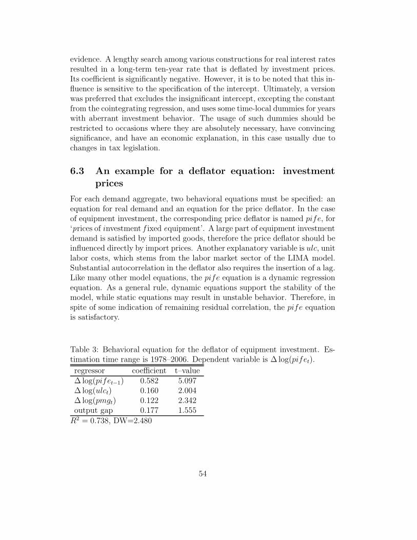
evidence. A lengthy search among various constructions for real interest ratesresulted in a long-term ten-year rate that is deflated by investment prices.Its coefficient is significantly negative. However, it is to be noted that this in-fluence is sensitive to the specification of the intercept. Ultimately, a versionwas preferred that excludes the insignificant intercept, excepting the constantfrom the cointegrating regression, and uses some time-local dummies for yearswith aberrant investment behavior. The usage of such dummies should berestricted to occasions where they are absolutely necessary, have convincingsignificance, and have an economic explanation, in this case usually due tochanges in tax legislation.

6.3 An example for a deflator equation: investment

prices

For each demand aggregate, two behavioral equations must be specified: anequation for real demand and an equation for the price deflator. In the caseof equipment investment, the corresponding price deflator is named pife, for‘prices of investment f ixed equipment’. A large part of equipment investmentdemand is satisfied by imported goods, therefore the price deflator should beinfluenced directly by import prices. Another explanatory variable is ulc, unitlabor costs, which stems from the labor market sector of the LIMA model.Substantial autocorrelation in the deflator also requires the insertion of a lag.Like many other model equations, the pife equation is a dynamic regressionequation. As a general rule, dynamic equations support the stability of themodel, while static equations may result in unstable behavior. Therefore, inspite of some indication of remaining residual correlation, the pife equationis satisfactory.

Table 3: Behavioral equation for the deflator of equipment investment. Es-timation time range is 1978–2006. Dependent variable is ∆ log(pifet).

regressor coefficient t–value∆ log(pifet−1) 0.582 5.097∆ log(ulct) 0.160 2.004∆ log(pmgt) 0.122 2.342output gap 0.177 1.555

R2 = 0.738, DW=2.480

54

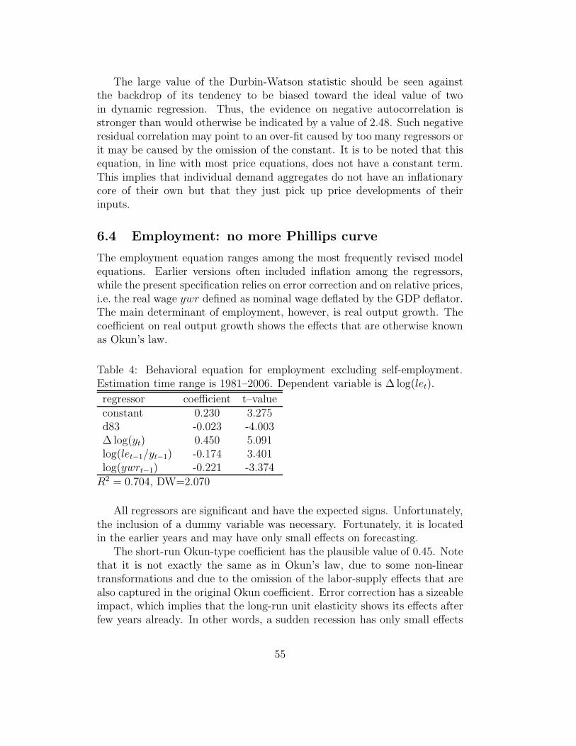
The large value of the Durbin-Watson statistic should be seen againstthe backdrop of its tendency to be biased toward the ideal value of twoin dynamic regression. Thus, the evidence on negative autocorrelation isstronger than would otherwise be indicated by a value of 2.48. Such negativeresidual correlation may point to an over-fit caused by too many regressors orit may be caused by the omission of the constant. It is to be noted that thisequation, in line with most price equations, does not have a constant term.This implies that individual demand aggregates do not have an inflationarycore of their own but that they just pick up price developments of theirinputs.

6.4 Employment: no more Phillips curve

The employment equation ranges among the most frequently revised modelequations. Earlier versions often included inflation among the regressors,while the present specification relies on error correction and on relative prices,i.e. the real wage ywr defined as nominal wage deflated by the GDP deflator.The main determinant of employment, however, is real output growth. Thecoefficient on real output growth shows the effects that are otherwise knownas Okun’s law.

Table 4: Behavioral equation for employment excluding self-employment.Estimation time range is 1981–2006. Dependent variable is ∆ log(let).

regressor coefficient t–valueconstant 0.230 3.275d83 -0.023 -4.003∆ log(yt) 0.450 5.091log(let−1/yt−1) -0.174 3.401log(ywrt−1) -0.221 -3.374

R2 = 0.704, DW=2.070

All regressors are significant and have the expected signs. Unfortunately,the inclusion of a dummy variable was necessary. Fortunately, it is locatedin the earlier years and may have only small effects on forecasting.

The short-run Okun-type coefficient has the plausible value of 0.45. Notethat it is not exactly the same as in Okun’s law, due to some non-lineartransformations and due to the omission of the labor-supply effects that arealso captured in the original Okun coefficient. Error correction has a sizeableimpact, which implies that the long-run unit elasticity shows its effects afterfew years already. In other words, a sudden recession has only small effects

55

on employment, while the full negative effects are felt if the recession doesnot end soon.

The negative effects of real wages, as the relative price of the productionfactor labor, are also quite strong. The variable ywr is the per capita grosswage divided by the GDP deflator. Technically, it counteracts the tendency ofemployment to grow in proportion to output, which would imply an absenceof technological progress. However, the long-run growth of real wage puts abrake on unlimited employment expansion. Thus, the employment equationis a stabilizing component in the LIMA model, even though its structure willcertainly have to be re-considered from time to time.

6.5 Theory and practice and the LIMA model

For many years, the LIMA model has proved a valuable backbone of the offi-cial IHS economic forecast. According to most comparative evaluations, theIHS economic forecast and that of its main competitor, the WIFO Institutefor Economic Research, are of a comparable quality. Usually, forecasts arepublished for the current and for the following year only. Once a year, amedium-term projection is also presented to the public.

The following points can be identified where the LIMA forecast does notcorrespond to textbook forecasting:

1. There is no sharp boundary between a sampling interval and a predic-tion interval. Most macroeconomic variables—exceptions are exchangerates and unemployment data—spend years in an intermediate stage,where they are known with an increasing degree of precision.

2. Often, predicting the final data, i.e. those that mark the endpoint of allrevisions by statistical agencies, is not targeted. For example, a forecastfor 2000 may become uninteresting in 2003, even when it perfectlycoincides with the final value.

3. The basis for prediction does not coincide with the estimation interval.For example, a forecast for 2007 is based on provisional data for alllagged variables from until 2006, while some model parameters maynot have been updated from values beyond 2005.

4. Add factors play a key role. Incoming information is reflected in size-able adjustment of residuals. Usually, zero-residuals forecasts are faroff the mark.

56

5. Exogenous variables for the prediction interval are updated on an adhoc basis. Some of these, however, correspond to information pro-vided by other institutions—for example, government spending—or byresearchers who use separate forecasting models.

6. All estimation is conducted by OLS, even when it is known that thisprocedure yields inconsistent estimates.

These points should not be interpreted as a critique of the current prac-tice. Rather, one may assume that the discrepancies between the textbookprediction approach and current practice follow a longer-run experience offorecasters on how to do forecasting efficiently. It may be interesting toextend the textbook framework, taking the practitioners’ approach into ac-count. This direction of research is still in an early stage.

57

7 Evaluating predictive accuracy

The question “How good is a forecast?” comprises two separate aspects:firstly, measuring predictive accuracy per se; secondly, comparing variousforecasting models. For example, if a variable is almost unpredictable, allforecasts are likely to be poor. Yet, a forecaster may still look for the bestforecast among the poor ones.

The most commonly reported measures of predictive accuracy are

1. mean squared prediction errors or a variant of them;

2. mean absolute prediction errors;

3. percentage measures, such as themean absolute percentage error (MAPE);

4. Theil coefficients;

5. significance measures, such as the Diebold-Mariano test statistic.

Additionally, some researchers, particularly in applied economics, use orsuggest qualitative accuracy measures. Chatfield focuses on such a mea-sure under the name of ‘Percent Better’. We should scrutinize each of thesesuggestions in turn.

Note that the words accuracy and precision are not synonyms. Precisionusually refers to the uncertainty of the forecast, for example measured by itsvariance, and does not imply accuracy.

7.1 Mean squared prediction errors

In the notation of Chatfield’s textbook, the prediction mean square errorPMSE is defined as

PMSE = m−1

N∑

t=N−m+1

(xt − xt−1 (1))2 .

In this form, PMSE evaluates out-of-sample one-step errors. N observa-tions are available, and the last m observations are used for evaluation. Theforecast xt−1 (1) is meant to be calculated on the basis of the observationsx1, . . . , xt−1 only, including parameter estimates. The formula is easily mod-ified for h–step errors with h > 1.

The PMSE formula does not specify m. Economic forecasters often tendto keep m/N small. For large m/N , the forecasts with small t are based onmodels estimated on short samples and thus be not representative. For small

58

m/N , however, the test sample may be too short to be a reliable indicator ofabsolute or relative accuracy. A potential modification would be to replacePMSE by a weighted MSE, with the weights increasing in t. This suggestionemphasizes the possibility that the true model may change over time. Then,the approximation by the prediction model toward the end of the sample ispotentially more important for forecasts beyond N than the approximationin the earlier portion.

As m → ∞, the PMSE should converge to a variance. Depending onthe properties of the DGP, if such a one is assumed to exist, that varianceshould be close to—though slightly larger than—the variance of the theoret-ical prediction error E (xt − E (xt|It−1))

2, where It−1 is an information setthat contains the history of the series x. That theoretical variance serves asthe benchmark for the construction of many statistical procedures, includingleast-squares estimation and AIC, which justifies the widespread usage of thePMSE.

The most common critiques of the PMSE are:

1. quadratic loss may not correspond to the forecaster’s loss function;

2. the PMSE depends on scales;

3. the PMSE is vulnerable to outliers.

The idea of a forecaster’s loss function is that forecast errors entail costs,in the sense that costs depend on

Eg (xt − xt−1 (1))

for some function g. Some authors even consider generalizations of the ex-pectation measure, as the costs may depend on time or on a nonlinear trans-formation of the vector of prediction errors, or on a more qualitative evalua-tion. The function should obey g (0) = 0 and g (x) > g (y) for x > y > 0 andx < y < 0. Otherwise, g may be asymmetric and it may converge to a finiteconstant as its argument approaches infinity. The main problem with theloss-function approach is that the true loss or cost function is rarely knownin practice. In some applications, even the existence of a cost function isuncertain, as the forecast may satisfy curiosity rather than serve as a basisfor actual immediate decisions. Therefore, only simple ad hoc loss functionsare considered usually, such as g (x) = x2 and g (x) = |x|. The first choiceyields the PMSE, the second one yields the mean absolute error, which isoccasionally preferred due to its robustness toward outliers.

59

The scale dependence of PMSE is not a problem, as long as a specificvariable x is in focus. If several variables are predicted using various proce-dures in each case, individual PMSEs should be weighted. A suggestion forweighting would be the sample variance of each series.

Often, instead of the PMSE, its square root is reported. While the PMSEcorresponds to a measure of variance, the root MSE is a measure of standarddeviation, which facilitates its interpretation. The transformation does notchange the ranking of models and predictions according to their accuracy,and it also does not remove any of the inherent problems of the PMSE.

7.2 Mean absolute prediction errors

In the same notation as above, the mean absolute error is defined as

MAE = m−1

N∑

t=N−m+1

|xt − xt−1 (1)| .

As m → ∞, the MAE should converge to E |xt − E (xt|It−1)| or a slightlylarger value, assuming this value exists. For a Gaussian world, this momentis proportional to the standard deviation, with a fixed proportionality factor.Also for other distributions, the absolute moment will measure the dispersionof the forecast errors.

The MAE is based on the loss function g (x) = |x|, which is more sensitiveto small deviations from 0 and much less sensitive to large deviations than theusual squared loss. Therefore, the MAE can be viewed as a ‘robust’ measureof predictive accuracy. The MAE tends to prefer forecasting procedures thatproduce occasional large forecast failures, while they are reasonably good onaverage. By contrast, the MSE tends to prefer forecasting procedures thatavoid large forecast failures, even though they produce a less satisfactory fitotherwise.

Because the estimation procedures are usually based on least-squares cri-teria, an emphasis on the MAE may involve a slight logical inconsistency.The best class of models is then selected according to a criterion that is dif-ferent from the one that selects among the different members of an individualmodel class.

60

7.3 Mean absolute percentage error

In the above notation, the mean absolute percentage error (MAPE) is definedby

MAPE = m−1N∑

t=N−m+1

∣

∣

∣

∣

xt − xt−1 (1)

xt

∣

∣

∣

∣

.

This definition answers complaints by some researchers that traditional crite-ria, such as PMSE and MAE, depend on the scaling of the variable x, whichmay be inconvenient if the criteria are used for comparing predictive accu-racy across different variables or different time ranges. Unfortunately, theMAPE achieves scale independence by a simple division by xt. This entailsa serious drawback.

Many economic variables, such as stock returns and most growth rates,vary around zero. Whenever xt = 0, the contribution at time point t andtherefore the MAPE are undefined. Even if xt is only approximately zero,the relative contribution of time point t will be enormous. Usually, there isno justification for preferring a high precision for small values of xt.

It is obvious that the MAPE is tuned to variables that live in an area thatis separated from zero by common sense. Economic examples would be themain aggregates of national accounts, such as fixed investment and privateconsumption.

Under the name of ‘rmse percent error’, Pindyck and Rubinfeld con-sider the direct squared-loss counterpart to the MAPE

m−1N∑

t=N−m+1

(xt − xt−1 (1))2

xt2.

This measure has properties that are similar to those of the MAPE, withwhom it shares most of its problems. While PMSE is more often reportedthan MAE, MAPE appears to be more popular than the above suggestion(see also Makridakis et al.).

In order to obtain a scale-free precision measure, it would be more ap-pealing to consider measures such as

∑N

t=N−m+1 (xt − xt−1 (1))2

∑N

t=N−m+1 (xt − x)2.

In this formula, the denominator measures the ‘total’ variation of x, whilethe numerator measures that part of the variation that has been accountedfor by the prediction procedure. Thus, the measure is reminiscent of theregression R2. Theil’s accuracy measures follow a similar idea.

61

7.4 Theil coefficients

The idea of Theil’s coefficients was to evaluate a forecast against the back-ground of a simple or primitive forecast. If a forecasting procedure is to betaken seriously, it should at least ‘beat’ the simple benchmark. Unfortu-nately, it is not always clear which benchmark to use. Theil used mainlyrandom-walk or no-change forecasts, while other researchers use autoregres-sive prediction or exponential smoothers instead.

The version of Theil’s coefficient that has been implemented into theEViews software is defined as

U =

√

∑N

t=N−m+1 (xt − xt−1 (1))2

√

∑N

t=N−m+1 x2t +

√

∑N

t=N−m+1 xt−1 (1)2.

For a ‘good’ predictor, the numerator will be small compared to the denom-inator. For a ‘bad’ predictor, both will be of similar magnitude. Theil’smeasures have often been criticized in the literature. They tend to yield im-plausible results in the sense that a predictor that optimizes them may haveundesirable properties and vice versa, at least under lab conditions. It is notso certain whether this is also true in practical applications.

7.5 Decomposing the mean squared error

According to the EViews manual and to Pindyck&Rubinfeld, the meansquared forecast error can be decomposed as

m−1∑

(xt − xt−1 (1))2 =

(

∑

xt−1 (1)− x)2

+ (sx − sx)2 +2 (1− rxx) sxsx.

Here, sx and sx are sample standard deviations of x and x, respectively, whilerxx is the sample correlation. Dividing the three parts by the total yields thebias proportion, the variance proportion, and the covariance proportion. Thenon-negative ‘proportions’ sum up to 1. According to the sources mentionedabove, the bias proportion tells how far the mean of the forecast is fromthe mean of the actual series. The variance proportion tells how far thevariation of the forecast is from the variation of the actual series. Finally,the covariance proportion measures the remaining unsystematic forecastingerrors.

The idea is that, if the forecast is ‘good’, the bias and variance proportionsshould be small so that most of the bias should be concentrated on thecovariance proportions. The informative value of the decomposition has notbeen accepted universally, however.

62

7.6 Diebold-Mariano statistics

The econometricians Diebold and Mariano were interested in a situationwhere a ‘cheap’ benchmark forecast is compared to a sophisticated forecast.A forecaster may prefer the cheap forecast up to a point where the sophisti-cated forecast shows its relative merits ‘significantly’. It is uncertain whetherthis situation is common in applications and empirical projects. Usually,various forecasting methods are considered and an optimum method is thenselected, while the cost of a forecast method plays little role. A complicatedforecasting method may even be selected if it only achieves a slight improve-ment on average. Some economic projects may even show an instinctive biastoward more sophisticated and costly methods, as these demonstrate theforecasting team’s skills.

Chatfield ranks among the few statisticians who criticized the nullhypothesis of these tests expressis verbis. That null hypothesis would bethat the expected difference in squared error (or some other loss moment) iszero. It is doubtful whether this null hypothesis is of central interest to thetypical forecaster.

Diebold&Mariano assume that the precision is basically measured byEg (xt − xt−1 (1)) and Eg (xt − xt−1 (1)) for two different forecasts x and xand a loss function g (.). Under the hypothesis that the difference is zero, itcan be shown that the test statistic

S1 =d

√

m−12πfd (0)

converges to a standard normal distribution as m → ∞. Here, d denotesthe sample average of dt = g (xt − xt−1 (1))− g (xt − xt−1 (1)). The elementfd (0) is a scale factor defined as the spectral density estimate of dt at thefrequency 0. An operable definition for fd (0) is

fd (0) = (2π)−1m−1∑

k=−m+1

w (k,m) γd (k) ,

where γd (k) is the sample autocovariance at lag k and w (.) is a kernel weightfunction that obeys certain consistency conditions, such as w (k,m) → 1 forfixed k and m→ ∞.

7.7 Qualitative measures

Sometimes, macro-economists maintain that they are less interested in theaccuracy of a real growth forecast than in forecasting ‘turning points’ of the

63

business cycle. It is uncertain whether such turning points exist outside ofthe official NBER chronology and economics textbooks. Similarly, a stockmarket analyst may be more interested in whether a specific security price isgoing to rise or to fall in the immediate future than in the numerical accuracyof the price prediction for the next day. Again, it is often uncertain whetherthe implied picture of longer sinusoidal swings in the security price with localmaxima (peaks) and local minima (troughs) corresponds to reality.

It is difficult to construct an accuracy measure for this type of loss func-tion, at least as long as the variable of concern x is quantitative. Someeconomists tend to ‘code’ and discretize some real-valued variables, suchthat ‘x increases’, ‘x decreases’, and ‘x remains approximately constant’ be-come the three events or ‘states’. Then, one may count the occurrences ofsuccesses and failures. The ‘better’ procedure is the one that yields moresuccesses or a larger success ratio. While the winning procedure may missthe exact value of x by far, its forecast for the ‘sign’ of x is reliable. Here,an inherent difficulty is the definition of ‘approximate constancy’. Instead ofsuccess ratios, one may also summarize this type of evidence in coincidencematrices.

A different kind of success ratio is suggested by Chatfield who, incomparing two methods A and B, counts the cases when A is closer to thetrue value and when B is closer. A forecaster who predicts many valuesclosely and misses a few ones by far, would attain a good ‘Percent Better’ratio. In this sense, Chatfield’s ‘Percent Better’ is a robust criterion andcomparable to the MAE. Note, however, that it is scale-independent, unlikethe MAE.

7.8 Forecast bias or mean error

The sample average of the prediction errors

m−1

N∑

t=N−m+1

(xt − xt−1 (1))

is also often reported for prediction experiments. It is not a real measure ofaccuracy, although it contains some important information. A forecast with alarge and systematic forecast bias could be improved by some straightforwardadjustment. In this sense, systematic over-prediction or under-predictionpoints to an inefficiency, or otherwise to an asymmetric loss function.

64

References

[1] Anderson, T.W. (1951) ‘Estimating linear restrictions on regressioncoefficients for multivariate normal distributions’. Journal of the Amer-ican Statistical Association 85, 813–823.

[2] Box, G.E.P., and G.M. Jenkins (1970) Time Series Analysis, Fore-casting, and Control. Holden-Day.

[3] Brockwell, P.J., and R.A. Davis (1991) Time Series: Theory andMethods. 2nd edition, Springer-Verlag.

[4] Cartwright, N. (1995) ‘Probabilities and experiments’. Journal ofEconometrics 67, 47–59.

[5] Chatfield, C. (2001) Time-series Forecasting. Chapman & Hall.

[6] Christoffersen, P.F., and Diebold, F.X. (1998) ‘Cointegrationand long-horizon forecasting’, Journal of Business & Economics Statis-tics 16, 450–458.

[7] Clements, M. (2005) Evaluating Econometric Forecasts of Economicand Financial Variables. Palgrave-Macmillan.

[8] Clements, M., and Hendry, D.F. (1998) Forecasting economic timeseries. Cambridge University Press.

[9] Clements, M., and Hendry, D.F. (1999) Forecasting Non-Stationary Economic Time Series. MIT Press.

[10] Dickey, D.A., and Fuller, W.A. (1979) ‘Distribution of the esti-mators for autoregressive time series with a unit root’ Journal of theAmerican Statistical Association 74, 427–431.

[11] Diebold, F.X., and Mariano, R.S. (1995) ‘Comparing PredictiveAccuracy’ Journal of Business and Economic Statistics 13, 253–263.

[12] Engle, R.F. (1992) ‘Autoregressive conditional heteroskedasticitywith estimates of variance of United Kingdom inflation’ Econometrica50, 987–1007.

[13] Engle, R.F., Hendry, D.F., and Richard, J.-F. (1983) ‘Exogene-ity’. Econometrica 51, 277–304.

[14] Engle, R.F., and Yoo, B.S. (1987) ‘Forecasting and Testing in Co-integrated Systems’, Journal of Econometrics 35, 143–159.

65

[15] Fair, R.C. (2004) Estimating How the Macroeconomy Works. HarvardUniversity Press.

[16] Fan, J., and Yao, Q. (2005) Nonlinear Time Series: Nonparametricand Parametric Methods. Springer.

[17] Franses, P.H. (1996) Periodicity and Stochastic Trends in EconomicTime Series. Oxford University Press.

[18] Franses, P.H., and VanDijk, D. (2000) Non-linear time series mod-els in empirical finance. Cambridge University Press.

[19] Gardner, E.S. Jr. (1985) ‘Exponential Smoothing: The State of theArt’ Journal of Forecasting 4, 1–28.

[20] Gardner, E.S.Jr., and McKenzie, E. (1985) ‘Forecasting trends intime series’ Management Science 31, 1237–1246.

[21] Granger, C.W.J. (1969) ‘Investigating Causal Relations by Econo-metric Models and Cross-Spectral Methods’ Econometrica 37, 424–438.

[22] Granger, C.W.J. (1989) Forecasting in Business and Economics.Academic Press.

[23] Harvey, A.C. (1989) Forecasting, Structural Time Series, and theKalman Filter. Cambridge University Press.

[24] Hylleberg, S., Engle, R.F., Granger, C.W.J., and Yoo, B.S.

(1990) ‘Seasonal integration and cointegration’ Journal of Econometrics44, 215–238.

[25] Johansen, S. (1995) Likelihood-Based Inference in Cointegrated VectorAutoregressive Models. Oxford University Press.

[26] Makridakis, S., Wheelwright, S.C., and Hyndman, R.J. (1998)Forecasting: Methods and Applications. 3rd edition, Wiley.

[27] Pindyck, R.S. and Rubinfeld, D.L. (1991). Econometric Models andEconomic Forecasts. 3rd edition, McGraw-Hill.

[28] Sims, C.A. (1980) ‘Macroeconomics and reality’. Econometrics 48, 1–48.

[29] Taylor, S. (1986) Modelling Financial Time Series. John Wiley &Sons.

66

[30] Terasvirta, T., Tjostheim, T., and Granger, C.W.J. ModellingNonlinear Economic Time Series. Oxford.

[31] Tong, H. (1990) Non-linear Time Series: A Dynamical Systems Ap-proach. Oxford University Press.

67