Forecasting Stock Market

Time Series

Regina Fuchs, 0103290

Richard Sellner, 0150085

Outline

• Description of the Data

• Model free procedures (Double

Exponential Smoothing, Holt-Winters

Method)

• Model based procedures (ARIMA,

GARCH)

• Forecasting and comparing the results

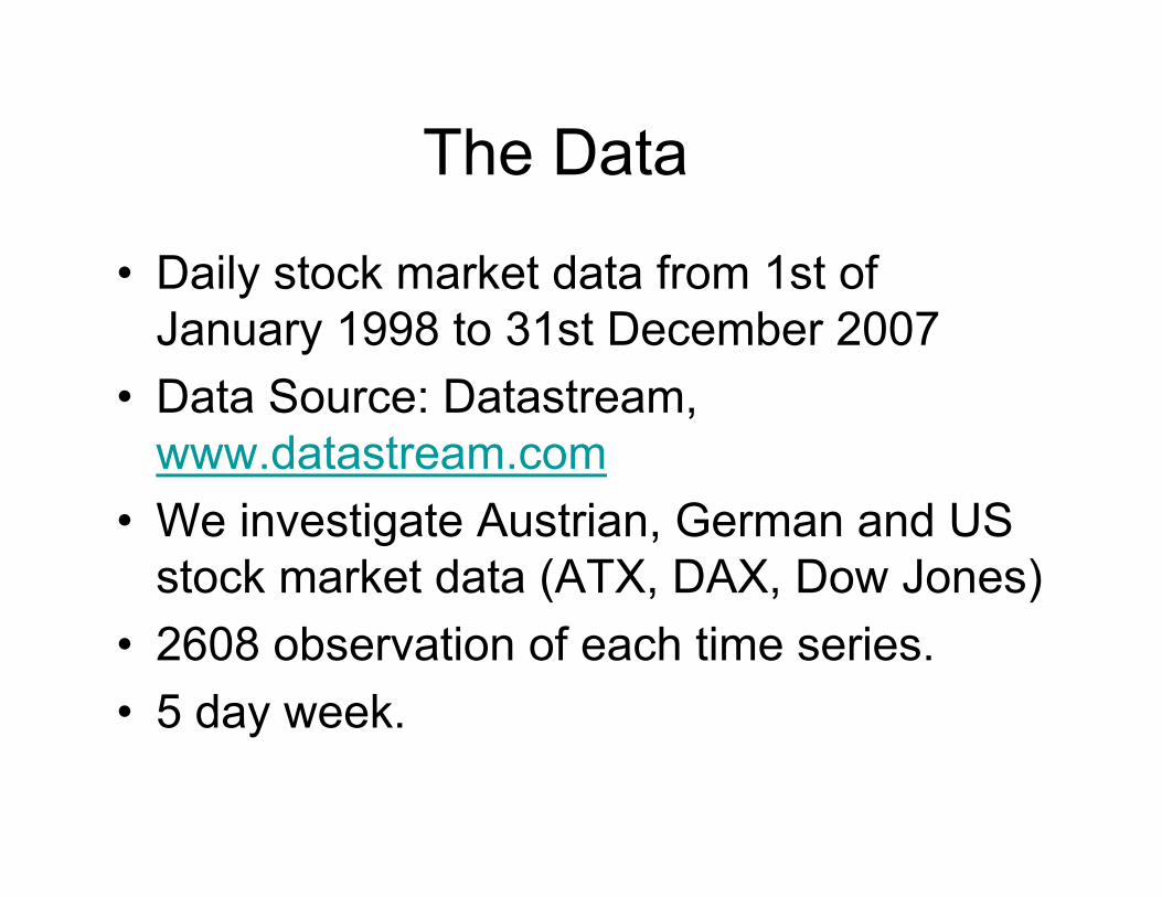
The Data

• Daily stock market data from 1st of

January 1998 to 31st December 2007

• Data Source: Datastream,

www.datastream.com

• We investigate Austrian, German and US

stock market data (ATX, DAX, Dow Jones)

• 2608 observation of each time series.

• 5 day week.

Graphical Representation

0

1000

2000

3000

4000

5000

6000

98 99 00 01 02 03 04 05 06 07

ATXINDX

2000

3000

4000

5000

6000

7000

8000

9000

98 99 00 01 02 03 04 05 06 07

DAXINDX

7000

8000

9000

10000

11000

12000

13000

14000

15000

98 99 00 01 02 03 04 05 06 07

DJINDUS

Augmented Dickey-Fuller

Test Stat. – Diff.Test Stat. – Level Index

-48.78-2.36DJ

-48.58-1.27 DAX

-17.832.57 ATX

Critical values: 1% (-3.43), 5% (-2,86). Time series seem to have unit roots.

Augmented Dickey Fuller test confirms this Hypothesis. For this reason, we

decided to compute 1st differences of the time series.

Time series in first differences

-.08

-.06

-.04

-.02

.00

.02

.04

.06

98 99 00 01 02 03 04 05 06 07

ATXD

-.12

-.08

-.04

.00

.04

.08

98 99 00 01 02 03 04 05 06 07

DAXD

-.08

-.06

-.04

-.02

.00

.02

.04

.06

.08

98 99 00 01 02 03 04 05 06 07

DJD

We used 01-01-98 to 31-12-06 to fit the

model and 01-01-07 to 31-12-07 for dynamic

forecast evaluation.

Double Exponential Smoothing

1

1

)1(

)1(

−

−

−+=−+=

ttt

ttt

TLT

LxL

αααα

• Time series are integrated of order one -> no single exponential smoothing.

• Literature suggests values of alpha between 0.1 and 0.3.

• We fixed value of alpha to 0.1, 0.3 and 0.9 respectively and additionally fitted an alpha to the data by minimizing MSE.

Holt-Winters Method

• We fixed an alpha of 0.1 and compared it with

the alpha E-Views suggests.

11

11

)1()(

))(1(

−−

−−

−+−=+−+=

tttt

tttt

TLLT

TLxL

ββαα

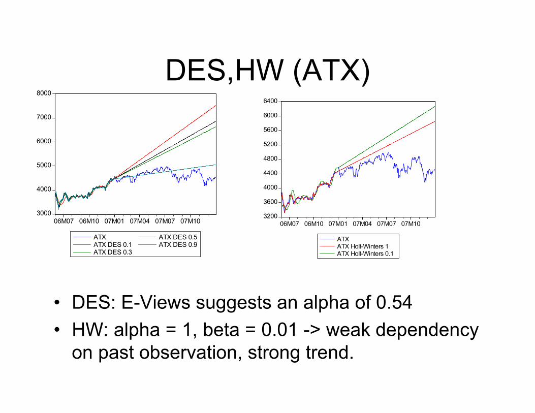
DES,HW (ATX)

• DES: E-Views suggests an alpha of 0.54

• HW: alpha = 1, beta = 0.01 -> weak dependency

on past observation, strong trend.

3000

4000

5000

6000

7000

8000

06M07 06M10 07M01 07M04 07M07 07M10

ATXATX DES 0.1ATX DES 0.3

ATX DES 0.5ATX DES 0.9

3200

3600

4000

4400

4800

5200

5600

6000

6400

06M07 06M10 07M01 07M04 07M07 07M10

ATXATX Holt-Winters 1ATX Holt-Winters 0.1

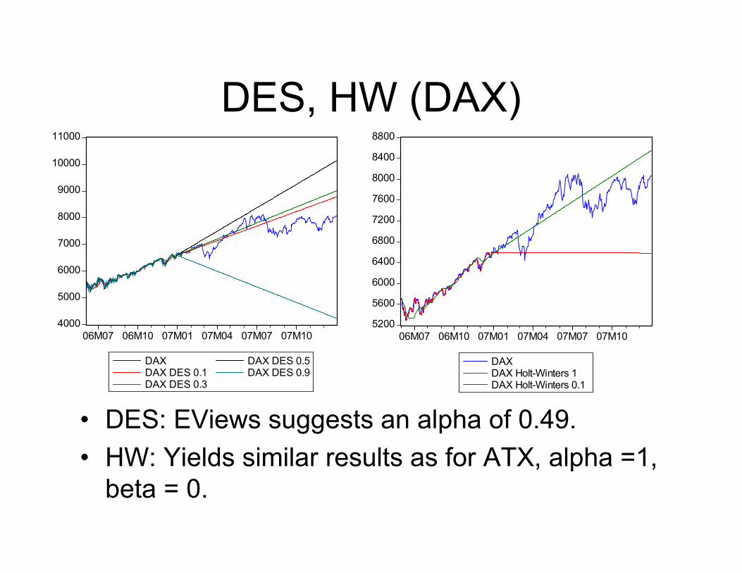
DES, HW (DAX)

• DES: EViews suggests an alpha of 0.49.

• HW: Yields similar results as for ATX, alpha =1,

beta = 0.

5200

5600

6000

6400

6800

7200

7600

8000

8400

8800

06M07 06M10 07M01 07M04 07M07 07M10

DAXDAX Holt-Winters 1DAX Holt-Winters 0.1

4000

5000

6000

7000

8000

9000

10000

11000

06M07 06M10 07M01 07M04 07M07 07M10

DAXDAX DES 0.1DAX DES 0.3

DAX DES 0.5DAX DES 0.9

DES, HW (DJ)

• E-Views suggests an alpha of 0.49

• HW: alpha = 0.99, beta = 0.

10000

11000

12000

13000

14000

15000

16000

06M07 06M10 07M01 07M04 07M07 07M10

DJDJ Holt-Winters 1DJ Holt-Winters 0.1

4000

6000

8000

10000

12000

14000

16000

06M07 06M10 07M01 07M04 07M07 07M10

DJDJ DES 0.1DJ DES 0.3

DJ DES 0.5DJ DES 0.9

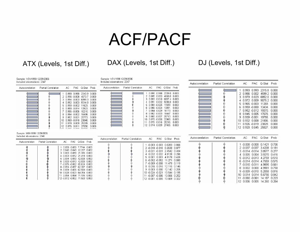
ACF/PACF

ATX (Levels, 1st Diff.) DAX (Levels, 1st Diff.) DJ (Levels, 1st Diff.)

ARIMA

• In order to fit a model to the time series we start visually inspecting the time series (ACF, PACF).

• The autocorrelations do not show a noticeable pattern.

• For this reason, we tried any ARIMA process from ARIMA (1,1,1) to ARIMA(8,1,8).

• We forecasted the model with the smallest AIC.

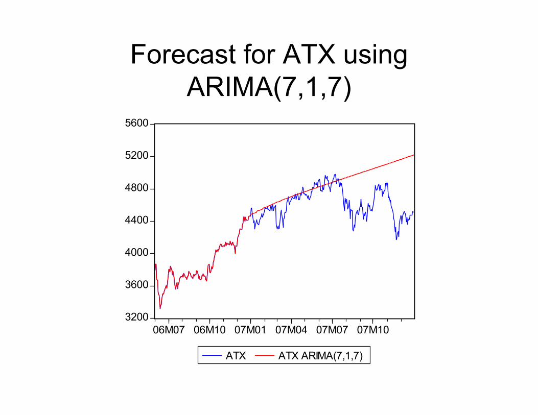
Forecast for ATX using

ARIMA(7,1,7)

3200

3600

4000

4400

4800

5200

5600

06M07 06M10 07M01 07M04 07M07 07M10

ATX ATX ARIMA(7,1,7)

Forecast DAX using ARIMA (8,1,8)

5000

5500

6000

6500

7000

7500

8000

8500

06M07 06M10 07M01 07M04 07M07 07M10

DAX ARIMA(8,1,8) DAX

Forecast for Dow Jones using

ARIMA (8,1,4)

10500

11000

11500

12000

12500

13000

13500

14000

14500

06M07 06M10 07M01 07M04 07M07 07M10

DJ DJ ARIMA(8,1,4)

Forecast using ARIMA-GARCH

models

1

2

1101

2)|( −−− ++==

+=

ttttt

tt

hhE

X

βεααεε

εµ

• Since Engel (1982) it has become very popular

in Finance to model volatility explicitly.

• We tried several ARIMA specifications of the

GARCH(1,1) model and performed a forecast for

the specification with the smallest AIC.

Forecast for ATX using

ARIMA(6,1,3) - GARCH

3000

3500

4000

4500

5000

5500

6000

06M07 06M10 07M01 07M04 07M07 07M10

ATX ATX ARIMA(6,1,3)-GARCH

Forecast for DAX using

ARIMA(3,1,3)-GARCH

5000

5500

6000

6500

7000

7500

8000

8500

06M07 06M10 07M01 07M04 07M07 07M10

DAX DAX ARIMA(3,1,3)-GARCH

Forecast Dow Jones using

ARIMA(2,1,1)-GARCH

10500

11000

11500

12000

12500

13000

13500

14000

14500

06M07 06M10 07M01 07M04 07M07 07M10

DJ DJ ARIMA(2,1,1)-GARCH

Evaluation: Root Mean squared

prediction error

∑+−=

−− −=

N

mNt

tt xxmRMSE

1

21

1 ))1(ˆ( 261=m 2608=N

ATX DAX DJ

DES 1268.63 1139.35 1018.56

DES 0.1 1648.60 432.92 732.51

DES 0.3 1136.65 1139.35 1018.56

DES 0.9 288.26 2325.69 5314.55

HW 701.65 995.74 753.30

ARIMA 373.66 788.96 550.21

GARCH 633.17 330.86 397.25

Thanks for your Attention!!