pids-bsp annual macroeconometric model for the philippines
TRANSCRIPT

DISCUSSION PAPER SERIES NO. 2020-16
APRIL 2020
PIDS-BSP Annual Macroeconometric Model for the Philippines: Preliminary Estimates and Ways Forward
Celia M. Reyes, Connie B. Dacuycuy, Michael Ralph M. Abrigo, Francis Mark A. Quimba, Nicoli Arthur B. Borromeo, Dennis M. Bautista, Jan Christopher G. Ocampo Lora Kryz C. Baje, Sylwyn C. Calizo Jr., Zhandra C. Tam, and Gabriel Iñigo M. Hernandez
The PIDS Discussion Paper Series constitutes studies that are preliminary and subject to further revisions. They are being circulated in a limited number of copies only for purposes of soliciting comments and suggestions for further refinements. The studies under the Series are unedited and unreviewed. The views and opinions expressed are those of the author(s) and do not necessarily reflect those of the Institute. Not for quotation without permission from the author(s) and the Institute.
CONTACT US:RESEARCH INFORMATION DEPARTMENTPhilippine Institute for Development Studies
18th Floor, Three Cyberpod Centris - North Tower EDSA corner Quezon Avenue, Quezon City, Philippines
[email protected](+632) 8877-4000 https://www.pids.gov.ph

PIDS-BSP Annual Macroeconometric Model for the Philippines: Preliminary Estimates and Ways Forward
Celia M. Reyes
Connie B. Dacuycuy
Michael Ralph M. Abrigo
Francis Mark A. Quimba
Nicoli Arthur B. Borromeo
Dennis M. Bautista
Jan Christopher G. Ocampo
Lora Kryz C. Baje
Sylwyn C. Calizo Jr.
Zhandra C. Tam
Gabriel Iñigo M. Hernandez
PHILIPPINE INSTITUTE FOR DEVELOPMENT STUDIES
April 2020 (Updated July 2020)

Abstract
Given new programs and policies in the Philippines, there is a need to formulate a
macroeconometric model (MEM) to gain more insights on how the economy and its sectors
are affected. This paper discusses the estimation of an annual MEM that will be used for policy
analysis and forecasting with respect to the opportunities and challenges brought about by new
developments. The formulation of an annual MEM is useful in assisting major macroeconomic
stakeholders such as NEDA and the BSP in their conduct of policy simulations,
macroeconomic surveillance, and economic analysis. Given this backdrop, PIDS and BSP have
collaborated to estimate an annual MEM, which has four blocks, namely, the real sector, fiscal
sector, trade sector, and monetary sector. Using an Autoregressive Distributed Lag model
approach, these sectors are modeled separately although the linkages with each other are
specified. These sectoral models are then put together and tests on the predictive accuracy of
the forecast of the overall model are conducted. Some ways to further improve the annual
MEM are provided.
Keywords: Autoregressive Distributed Lag Model, Macroeconometric Model, National
Income Accounting

Table of Contents
1. Introduction .......................................................................................................... 1
2. Modelling the Philippine economy: A 4-sector model ...................................... 2
2.1. Real Sector ...................................................................................................... 3
2.2. Fiscal Sector .................................................................................................... 4
2.3 Trade Sector ..................................................................................................... 5
2.4 Monetary Sector ................................................................................................ 5
3. Empirical strategy ................................................................................................ 6
3.1 Autoregressive Distributed Lag Model .............................................................. 6
3.2. Determination of long-run relationship and pre- and post-estimation routines . 7
4. Preliminary results ............................................................................................... 7
5. Model Validation ................................................................................................... 8
6. Ways forward ........................................................................................................ 8
7. References ............................................................................................................ 9
List of Appendix
APPENDIX 1: Mapping of variables ......................................................................... 11
APPENDIX 2: Lists of variables, definition, and sources .......................................... 12
APPENDIX 3: Equation-by-equation estimates ........................................................ 23
APPENDIX 4: Test of the predictive accuracy ........................................................ 199
APPENDIX 5: Documentation of creating consistent data series ........................... 203

1
PIDS-BSP annual macroeconometric model for the Philippines:
Preliminary estimates and ways forward
Celia M. Reyes, Connie B. Dacuycuy, Michael Ralph M. Abrigo,
Francis Mark A. Quimba, Nicoli Arthur B. Borromeo, Dennis M. Bautista,
Jan Christopher G. Ocampo, Lora Kryz C. Baje, Sylwyn C. Calizo Jr.,
Zhandra C. Tam, and Gabriel Iñigo M. Hernandez1
1. Introduction The Philippine Development Plan 2017-2022 has identified several strategies that need to be
implemented in order to improve the ability of the fiscal sector to promote development and
inclusive growth. Given this, the Philippine Institute for Development Studies (PIDS) has
collaborated with the Bangko Sentral ng Pilipinas (BSP) to build a macroeconometric model
(MEM). The formulation of an annual MEM is useful in assisting major macroeconomic
stakeholders such as NEDA and the BSP in their conduct of policy simulations,
macroeconomic surveillance, and economic analysis.
The development of the PIDS-BSP Annual MEM is useful in policy analysis given various
developments at the global and national stage in the past two decades. At the global stage, the
country has seen the Global Financial Crisis in 2008, the election of leaders abroad with
inward-looking policies, and the trade tension between US and China among other things,
unfold. At the national stage, the Philippines has experienced an average gross domestic
product (GDP) growth rate of over 6 percent since 2011. It has witnessed the boom of the
Information Technology-Business Process Outsourcing (IT-BPO) sector in the early 2000 and
has experienced damages of calamitous proportion in the face of typhoon Ondoy in 2009 and
the super typhoon Yolanda in 2013. Several policies such as the government’s infrastructure
program (dubbed as the Build Build Build) and the tax reform program (Tax Reform for
Acceleration and Inclusion) are also underway.
In the past, several MEMs in the Philippines had been done. One of these was the PIDS-NEDA
Annual MEM, which had several versions (see Constantino and Yap 1988; Constantino et al
1990; Reyes and Yap 1993). The main objective of these MEMs was to provide a coordinated
framework for the formulation of medium-term development plans for the Philippines. It was
extensively used during the negotiations involving the country’s external debt in the early years
of the Aquino administration in the late 1980s. It was also used to evaluate the impact of
stabilization policies in the Philippine economy.
Reyes and Yap (1993) version of the PIDS-NEDA Annual MEM followed a structuralist
approach to macroeconomics, which subscribed to a less than full-employment equilibrium. In
this approach, output is primarily determined from the supply side although the demand side
also has a role. There were four major sectors in this MEM: (1) Real Sector, (2) Fiscal Sector,
(3) Financial Sector, and (4) External Sector. The model focuses on the Real Sector, which has
four sub-blocks including production, expenditure, income, wages/employment. GDP was
1 The first author is President of the Philippine Institute for Development Studies (PIDS). The next three authors are senior
research fellows while the fifth author is a former supervising research specialist also at PIDS. The sixth and seventh authors are deputy director and bank officer, respectively, at the Bangko Sentral ng Pilipinas. The next three authors are research analysts while the last author is a former research analyst at PIDS, as well.
2
determined by the interaction of the production side and the expenditure side while government
spending was assumed to be exogenous. This strong link between the production and
expenditures was a significant departure from earlier MEMs such as those in Villanueva
(1977). Meanwhile, the financial sector determined the money supply and the interest rates,
which were used in the real sector to determine output while the trade sector was disaggregated
into various components. This version of the PIDS-NEDA Annual MEM had accounted for the
role of infrastructure in output determination and the effect of public capital expenditures on
power generation. Power outages had been a big issue in the early 1990s.
The PIDS-BSP Annual MEM closely follows the PIDS-NEDA Annual MEM in its attempt to
provide a close link between the production and expenditure sub-blocks of the real sector.
However, the former has modeled a more disaggregated household final consumption
expenditure in order to analyze the effects of consumption-specific taxes and duties. In
addition, the wages are also disaggregated to provide better information in the country’s
production structure. The external sector reflects an updated disaggregation of the goods and
services traded by country highlighting the more significant subsectors of the country like
Computer Services Exports (BPO) and Tourism. Compared to earlier Philippine MEMs, the
accounts in the fiscal sector are also more finely disaggregated and follow more closely the
general government income and outlay accounts of the Philippine System of National
Accounts.
2. Modelling the Philippine economy: A 4-sector model
Consistent with Reyes and Yap (1993), the theoretical framework of the model is influenced
by the structuralist approach to macroeconomics, which takes into account the economy’s
structural features into policy analysis. The structuralist approach subscribes to the notion of
an equilibrium at less than full employment (Taylor, 1991), which to a great extent is observed
in the Philippine economy. In 2018, the unemployment and underemployment rates in the
country are 5.5% and 17%, respectively.
Following the structuralist approach to obtain equilibrium at less than full-employment, the
determination of prices in the sectors follow the fix-price/flex-price method (Hicks, 1985). In
the flex-price system, the demand for and supply of commodities determine the price level,
which inform producers on whether to expand or contract the quantities they will produce. In
the fix-price system, prices can remain unchanged over a period of time although adjustments
will eventually be made to address the surplus (shortage) through output contraction
(expansion). Sectors are assumed to have excess capacity and producers are operating under a
non-competitive scenario where producers practice mark-up pricing. The agricultural sector is
assumed to follow the flex-price system while the industrial and services sectors are assumed
to follow the fix-price system. This assumption has been made by Reyes and Yap (1993) and
is also adapted in this version of the PIDS-BSP Annual MEM as its implications are still
observed in the structure of the Philippine economy today.
Similar to Reyes and Yap (1993), the economy is assumed to have four sectors, namely, the
real sector, fiscal sector, trade sector, and monetary sector. This version of the PIDS-BSP
Annual MEM has 132 behavioral equations, 65, 20, 30, and 17 of which pertain to the real
sector, fiscal sector, trade sector, and monetary sector, respectively. The production and
expenditure sub-blocks of the real sector are linked by including some household final
consumption expenditures into the determination of some of the sectoral gross value added.
3
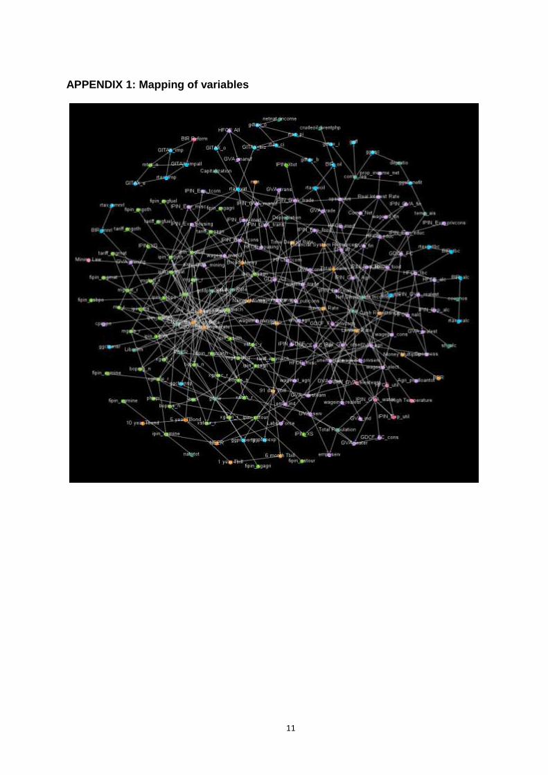
The real sector is also linked with the fiscal sector through the inclusion of interest and reverse
repurchase rates (RRR) into the production subsector and with the external sector through
relevant import and export items (see Appendix 1 for mapping of variables).
2.1. Real Sector
The real sector is made up of four subsectors: production, expenditure, income, and
wage/employment. The aggregation of the GVA or the expenditure items can be used to solve
for the GDP. These two subsectors are linked through the inclusion of specific expenditure
items into the GVA specifications.
The production subsector has eleven groups: agriculture, industry (disaggregated into
construction, electricity and steam, water, manufacturing, mining, and finance), and services
(real estate, trade, transportation, and other services). An indicator for weather patterns
(proxied by the deviation of rainfall from its long-run average) also affects the agricultural
production through the implicit price index. The GVA in each subsector is affected by its
corresponding implicit price index and is closely linked with the monetary sector through the
real effective exchange rate and RRR and with the external sector through the exports and
imports of specific items. Meanwhile, the implicit price index of each group is affected by its
compensation index per employee. Some of the implicit price indices, such as those of real
estate and other services, are also linked with the monetary sector through the lending rate
while the implicit price indices of construction and manufacturing are linked with the external
sector through the imports of fuel and machinery.
On the expenditure side, the HFCE has ten groups: (a) alcoholic beverages, (b) non-alcoholic
beverages, (c) tobacco, (d) education, (e) food, (f) medical, (g) housing, (h) transportation and
communication, (i) utilities, and (j) miscellaneous (which covers the rest of the HFCE items).
Each sector is affected by its corresponding price index and the disposable income. In turn, the
price indices are affected by the price of imports, real interest rate, and exchange rate to pick
up cost effects. The link of expenditure side with the fiscal sector is established through the
inclusion of tax rates on prices. In this version of the PIDS-BSP Annual MEM, the effective
tax rate of alcoholic beverages and import duties affect the implicit price of food while the
import duty affects the implicit price of medical goods.
Among the components of Gross Domestic Capital Formation (GDCF), fixed capital such as
construction expenditures (private and public) are modeled as functions of financial variables
such as the real interest rate, exchange rate, and T-bill rate. Change in inventory, on the other
hand, is affected by the $/PhP exchange rate, inflation rate, and capital depreciation.
On the income side, net disposable income is the sum of net compensation of domestic
employees, net operating surplus from resident producers, property income, net compensation
from the rest of the world, taxes on production and on imports and subsidies, and total transfers
from abroad. The first three components are modeled in the real sector and are affected by
variables from financial sector such as the real interest rate, exchange rate, and inflation.
In terms of employment, that of the agricultural sector is affected by the sectoral wage indices
while that of the industry is affected by external factors such as the imports of machinery to
account for the sector’s increasing intensity of capital use and the exports of BPO services,
which have been booming in recent years. Population also plays a role in the determination of
sectoral employment. Meanwhile, the unemployment rate is affected by the labor force while
4
the labor force is affected by the country’s exports of services and use of government income.
Consistent with Okun’s Law, unemployment rate is affected by wages.
2.2. Fiscal Sector
The econometric models in this sector is designed to simulate and/or forecast general
government net lending (borrowing) based on separate time-series models of the different
sources of government revenues, and on programmed government expenditures taken
exogenously. This module interacts with the rest of the PIDS-BSP Annual MEM through its
linkages with other institutional sectors of the economy, namely, households and non-profit
institutions serving households, corporations, and the external sector. It also interacts with the
monetary sector directly through general government debt and debt servicing, and indirectly
through the latter’s influence on other institutional sectors. More specifically, this block
interacts with the rest of the sectors by using variables from other model blocks, e.g. prices
from the real sector, interest rates from the monetary sector, and exchange rates from the
external sector, as inputs to predict different government accounts (e.g. taxes and other
revenues). Variables form the government sector, on the other hand, are important determinants
of outcomes in the real sector (e.g. GDP).
Different streams of tax revenues are modelled separately as a function of effective tax rates
and the tax base for the good and/or service to be taxed. The effective tax rates are estimated
using individual tax rates for separate goods and services weighted by either value or quantity
of each good or service that is taxed, depending on the type of tax. For personal income tax
revenues, for example, the time series of effective tax rates are calculated using the distribution
of household incomes from the triennial Family Income and Expenditure Survey. Missing
values are linearly imputed. Its tax base, on the other hand, are proxied by annual aggregate
compensation of employees and gross operating surplus estimates from the national accounts.
In this version of the PIDS-BSP Annual MEM, the following tax revenues from the following
sources are modelled separately: (a) import taxes and duties, (b) indirect taxes on business and
occupations, (c) other indirect taxes, (d) excise taxes on domestic products, (e) direct taxes on
business, (f) direct taxes on individuals, and (g) other indirect taxes. Excise taxes are
disaggregated further by commodity, including alcoholic beverages, tobacco, petroleum, and
minerals. Other government revenues, such as (h) social contributions, (i) property income,
and (j) compulsory fees and fines, are also modelled separately using a similar approach used
for government tax revenues. These other government revenues are modelled as a function of
the effective contribution rate, whenever available, and the effective revenue base of these
accounts, or its proxy variables.
Following Yap (2000), government final consumption expenditures (GFCE) are taken as
exogenous in the model although a bridge equation linking actual government expenditures on
personal services, and maintenance and other operating expenditures with GFCE is specified
to ensure internal consistency. Other expenditures, such as on social security benefits and
property expense, are modelled using a similar approach to (h) and (i) above.
General government savings may be derived using estimates/forecasts of the above variables.
When combined with other government accounts, such as the GDCF and net asset holdings,
annual government surplus, and debt stocks may also be calculated. As such, the fiscal sector
is able to capture the influence of different macroeconomic factors on the debt position of the
5
government through these factors’ direct and indirect effects on different government incomes
and expenditures.
2.3 Trade Sector
The trade sector models the flow of goods, services, capital, and transfers in and out of the
country. The different sectors of imports and exports are modelled using demand equations.
On the export side, the export demand equation (EDE) models each subsector good/service as
a function of foreign demand (usually proxied by world GDP), the price index of the subsector,
and relevant exchange rates. The goods for which the EDE is estimated include the key exports
of the country in recent years, namely, (a) electronic components, (b) agricultural exports, (c)
minerals, and (d) other manufactured goods exports (residual). In recent years, the export of
services has grown significantly. As such, the EDE models of (a) computer services exports
(BPO), (b) tourism, and (c) other services exports (residual) are also included.
On the import side, the import demand equation (IDE) models each subsector good/service as
a function of domestic demand (captured by household consumption, investment, and/or
government spending), the import price, and relevant exchange rate. The IDE models of (a)
machinery and equipment, (b) material inputs, (c) fuel, (d) agricultural products, and (e) other
imports (residual) are also included.
This disaggregation of exports and imports allows the external sector block to capture changes
in demand for key Philippine goods and services brought about by the exogenous factors. The
impact of sharp increases in the prices of key production inputs such as fuel is also modelled
through the imports equation.
The export and import price deflators are specified as functions of domestic prices and previous
price deflators. In addition, tariff rates affect the import price deflators. Finally, the total exports
and imports are converted to dollars using the US$-PhP exchange rate. These aggregate
accounts enter the Balance of Payments.
2.4 Monetary Sector
The monetary sector attempts to capture the major channels of the monetary policy
transmission mechanism. Monetary policy decisions affect output and inflation through the
monetary transmission process that conventionally operates through the interest rate channel,
credit channel, exchange rate channel, the asset price channel, and the expectations channel.
These channels are not mutually exclusive as the effect of one channel could amplify or
moderate the effect of another channel. It should be noted that these channels are not invariant
over time since they evolve alongside changes in the overall economic and financial conditions.
The overnight RRR, which serves as the BSP’s key policy rate, is estimated as the primary
driver of domestic interest rates. A change in the BSP’s monetary policy stance is transmitted
through the various interest rates that affect overall economic activity. The policy rate is
estimated to affect savings, time deposit, and lending rates of banks, which influence the
consumption and investment decisions of households and firms. Moreover, changes in the
policy rate is transmitted across the different maturities of the government’s yield curve, which
influence fiscal conditions.
6
The exchange rate channel is particularly relevant for small open economies like the
Philippines especially with greater integration of commodities, services and financial markets
alongside a flexible exchange rate regime. Exchange rates are primarily determined by interest
rate and inflation differentials. Movements in the exchange rates influence the price of
domestic and foreign goods and services, which influence aggregate demand and inflation.
The model also captures the credit channel of monetary policy by tracing the impact of changes
in the policy rate and the reserve requirements ratio (RRR) on domestic liquidity and the
banking system’s credit activity. In this channel, the traditional interest rate channel is
amplified and propagated by how changes in policy rate affect the availability and cost of
credit.
3. Empirical strategy
3.1 Autoregressive Distributed Lag Model
The PIDS-BSP Annual MEM will be estimated using an Autoregressive Distributed Lag
(ARDL), which is represented by the following:
𝑦𝑡 = 𝛼𝑡 + ∑𝛼𝑖𝑦𝑡−1 + ∑∑𝛽𝑘𝑖𝑥𝑘𝑡−1 + 𝑢𝑡
𝑛
𝑖=0
𝑚
𝑘=1
𝑛
𝑖=1
Equation 1
Here, 𝑢𝑡 is assumed to be a white noise error: zero mean [𝐸(𝑢𝑡) = 0, constant variance
[𝐸(𝑢𝑡2) = 0, and serially uncorrelated [𝐸(𝑢𝑡𝑢𝑡−𝑠) = 0]. ARDL has various advantages. It has
an Error Correction representation, which allows for the analysis of short-run and long-run
relationships of variables. It is a dynamic single equation, which makes for easy
implementation and interpretation. It can be used in series with orders 0 [I(0)] or 1 [I(1)] and it
can accommodate different lags in 𝑥 and 𝑦.
Given a one explanatory variable 𝑥 with one lag, equation 1 becomes
𝑦𝑡 = 𝛼0 + 𝛼1𝑦𝑡−1 + 𝛽0𝑥𝑡 + 𝛽1𝑥𝑡−1 + 𝑢𝑡
Equation 2
Equation 2 can be reparameterized to get the following:
𝛥𝑦𝑡 = 𝑐 + (𝛼1 − 1)𝑦𝑡−1 + 𝛽0𝛥𝑥𝑡 + (𝛽1+𝛽0)𝑥𝑡−1 + 𝑢𝑡 Equation 3
𝛥𝑦𝑡 = 𝑐 + 𝜃0[𝑦𝑡−1 + 𝜃1𝑥𝑡−1] + 𝛽0𝛥𝑥𝑡 + 𝑢𝑡
Equation 4
Equation 3 is ARDL in differenced form while equation 4 is the ECM representation of the
ARDL in differenced form where 𝜃0 = 𝛼1 − 1 and 𝜃1 =𝛽1+𝛽0
−𝜃0 . 𝜃0 = 𝛼1 − 1 is the speed of
adjustment to the steady state and −1 < 𝜃0 < 0 for dynamic stability. θ1 is the long-run
multiplier while β0 is the short-run multiplier.

7
3.2. Determination of long-run relationship and pre- and post-estimation routines
The ARDL approach can be used to model a mix of I(0) and I(1)series, which can be
implemented using the bounds test procedure developed by Pesaran et al. (2001). The test for
the existence of a significant long-run relationship is an F-test for the variables in lagged levels
or 𝐻0: 𝜃0 = 𝜃1 = 0. The bounds test has the following rules:
• (computed) F-statistic < the lower bound: H0 of no long-run relationship between the
variables cannot be rejected.
• (computed) F-statistic > the upper bound: H0 of a no long-run relationship is rejected.
• F-statistic falls within the range of the lower and upper bounds: The test is inconclusive.
Since the bounds test is no longer applicable in the presence of series with higher order, unit
root tests have been implemented and results indicate that all series are either I(0) or I(1). All
variables are in natural logarithms (see appendix 2 for sources and computation).
A battery of tests has been conducted to ensure the adequacy of each specification. A white
noise test (Portmanteau test) is implemented to test the adequacy of the model. In this test, the null hypothesis is that residuals follow a white noise process. This means that the residuals have
zero mean, constant variance, and are serially uncorrelated. Nevertheless, additional tests for serial
correlation (Durbin-Watson test) and heteroscedasticity (Breusch-Pagan test) are implemented.
The null hypothesis of the former is that there is no serial correlation while the null hypothesis of
the latter is that the residual has constant variance. Results of these tests are found in Appendix 3.
4. Preliminary results
The preliminary equation-by-equation estimates confirm the expected signs. All the
specifications have passed the battery of tests and the bounds test indicate that the variables
have long-run relationships. Some pertinent results based on the equation-by-equation
estimates include the following:
1. The supply side of the agricultural production is not very sensitive to domestic prices,
as output cannot increase easily to meet demand. It is, however, more sensitive to the
prices of exported agricultural exports, with an increase in the price of foreign
agricultural products resulting in a higher GVA for agricultural product.
2. The price indices in the production side are affected by costs in the other sectors,
including the exchange rates, lending rates, as well as by labor market costs such as the
sectoral wage indices.
3. The HFCE positively affects the GVA of manufacturing, trade, and transportation.
4. Food prices is negatively affectively by the country’s openness. This potentially
captures the positive effect of the country’s liberalization of its agricultural markets.
5. The prices of tobacco and medical goods are positively affected by tobacco tax rate and
import duties, respectively.
6. Investment is sensitive to various measures of interest rate.
7. Operating surplus is negatively affected by the price of capital (interest rates) and
positively by the level of investment in capital formation.
8
8. Capitalization increases the employment in the industry sector while developments in
the BPO, such as increased exports of BPO services, decreases the employment in the
industry sector.
9. The long-run parameters on tax rates in the fiscal sector ARDL models are positive and
statistically significant, implying that the Philippines is still on the upward- sloping side
of the Laffer curve over the estimation period. That is, having higher tax rates may
increase government tax income holding other things the same. However, the
coefficient must be interpreted with caution as there may be other unobservable factors
that may confound the parameter estimates.
10. Models of many government sector accounts have poor fit when using the baseline tax
rate and taxable amount as predictors. This suggests that there may be other factors in
play, e.g. collection effort, in determining these accounts.
11. Real exports of goods (Agriculture, Mineral Exports and Other Goods) and Real exports
of services (Tourism, Other Services) are negatively affected by prices and positively
affected by the growth of world economy.
12. In the long run, real exports are positively affected by the depreciation of the real
exchange rate while real imports are negatively affected by it.
5. Model Validation
There are several measures that can be looked into to determine the extent of the accuracy of
the forecast of the MEM. This PIDS-BSP Annual MEM version looked into the mean absolute
percentage error (MAPE), which is computed as 𝑀𝐴𝑃𝐸 =1
𝑛∑ |
𝐴𝑐𝑡𝑢𝑎𝑙𝑡−𝑃𝑟𝑒𝑑𝑖𝑐𝑡𝑒𝑑𝑡
𝐴𝑐𝑡𝑢𝑎𝑙𝑡|𝑛
𝑡=1 . A lower
MAPE indicates a better predictive performance of the forecast system.
Table 1 in appendix 4 shows the in-sample MAPE statistics (2002-2016) of key variables as
well as the out-of-sample forecasts for 2017 and 2018. It can be seen that the MAPEs of the in-
sample forecasts for the production and expenditures subsectors of the real sector block are
relatively low at less than 5%. However, the GDCF and some of its components have relatively
high MAPEs (greater than 10%). Similarly, the forecasts of some variables in the fiscal sector
also have relatively high MAPEs including the import duty, excise tax on domestic product,
income taxes on business and individual, total government savings, and total government
surplus. The forecasts of some of the external and financial variables also have high MAPEs.
These observations are carried over to the 1-step ahead forecasts (2017) and 2-step ahead
forecasts (2018), with the latter having higher MAPEs than the former.
6. Ways forward
While the challenges of data collection needed for this type of modeling strategy have been
addressed, several important areas should be looked into. These include the following:
1. There is a need to strengthen the link of the real sector with the fiscal sector. This can
be done by ensuring that relevant taxes are included in the specifications of the implicit
price index (IPIN) of the disaggregated HFCEs and their signs conform to a priori
expectations.
2. There is a need to strengthen the link of the production and expenditure sub-blocks of
the real sector. In the current version, only the GVAs of manufacturing, transportation,

9
and trade are affected by the relevant HFCEs. The HFCE-education, for example, can
be used as an explanatory variable of the GVA of other services while the HFCE-food
can be used as an explanatory variable of the GVA of agriculture.
3. While the current model incorporates the relationship between the GVA and IPIN of
exports or imports in some equations (e.g. Agriculture GVA), there is a need to
strengthen the linkage of the export and/or import price indices and the relevant sectors
which may be affected by the change in these prices. For instance, the GVA of
manufacturing may be affected by the IPINs of imports of material inputs, machinery,
and fuel.
4. There is a need to strengthen the specifications and linkages of the private and public
investments. In the current version, there is no link to analyze crowding-in and
crowding-out effects of public investments.
5. The specification of cash remittances can be improved by including the world economic
growth or the weighted growth of countries where majority of OFWs are deployed.
6. There is a need to streamline the specifications included in the monetary sector.
Currently, the model has several T-bill rates although only the 91-day T-bill rate is used
in the real sector. In addition, the feedback between the real sector with the monetary
sector is somewhat weak. While the exchange rate, lending rate, real interest rate, RRR,
and the 91-day T-bill rate are included in the real sector, only the GDP is used in the
monetary sector, specifically, in the US$ and JPY nominal exchange rates.
7. The equations for the exchange rates of USD, JPY, and CNY should also be more
theoretically consistent by focusing on interest rate and inflation differentials.
8. There is a need to analyze the predictive accuracy of the forecasts through the use of
other metrics such as the root mean squared error (RMSE), mean absolute prediction
error (MAE), and Theil coefficient.
9. The forecasting accuracy of the fiscal sector models may be improved by expanding
the sector’s linkages with the rest of the PIDS-BSP MEM. This may be difficult to
implement, however, because of the rather short temporal coverage of many of the input
data series. Expanding the historical coverage of these series may be an important step
moving forward.
7. References
Constantino, W. and Yap, J. (1988). The impact of trade, trade policy and external shocks on
the Philippine economy based on the PIDS-NEDA macroeconometric model.
Philippine Institute for Development Studies Working Paper No. 1988-29. Retrieved
from serp-p.pids.gov.ph
Constantino, W., Yap, J., Butiong, R, and dela Paz, A. (1990). The PIDS-NEDA annual
macroeconometric model version 1989: A summary. Philippine Institute for
Development Studies Working Paper No. 1990-13. Retrieved from serp-p.pids.gov.ph
Frisch, R. (1933). Propagation problems and impulse problems in dynamic economics.
Economic Essays in Honour of Gustav Cassel. Frank Cass. London
Hicks, J. (1985). Method of dynamic economics. Oxford: Macmillan.
Orbeta, A. (2002) Education, labor market, and development: A review of the trends and issues
in the Philippines for the past 25 Years. PIDS DP 2002-19.

10
Pesaran, M. H., Shin, Y. and Smith, R. J. (2001). Bounds testing approaches to the analysis of
level relationships. Journal of Applied Econometrics, 16: 289-326.
Reyes, C. and Yap, J. (1993). Reestimation of the macroeconomic model. Philippine Institute
for Development Studies Discussion Paper Series. Retrieved from serp-p.pids.gov.ph
Taylor, L. (1983). Structuralist macroeconomics: applicable models for the third world. New
York: Basic Books.
Villanueva, D. (1977). A semi-annual macroeconometric model of the Philippines, 1967-1976.
IMF Departmental Memoranda Series 77/89.
11
APPENDIX 1: Mapping of variables
12
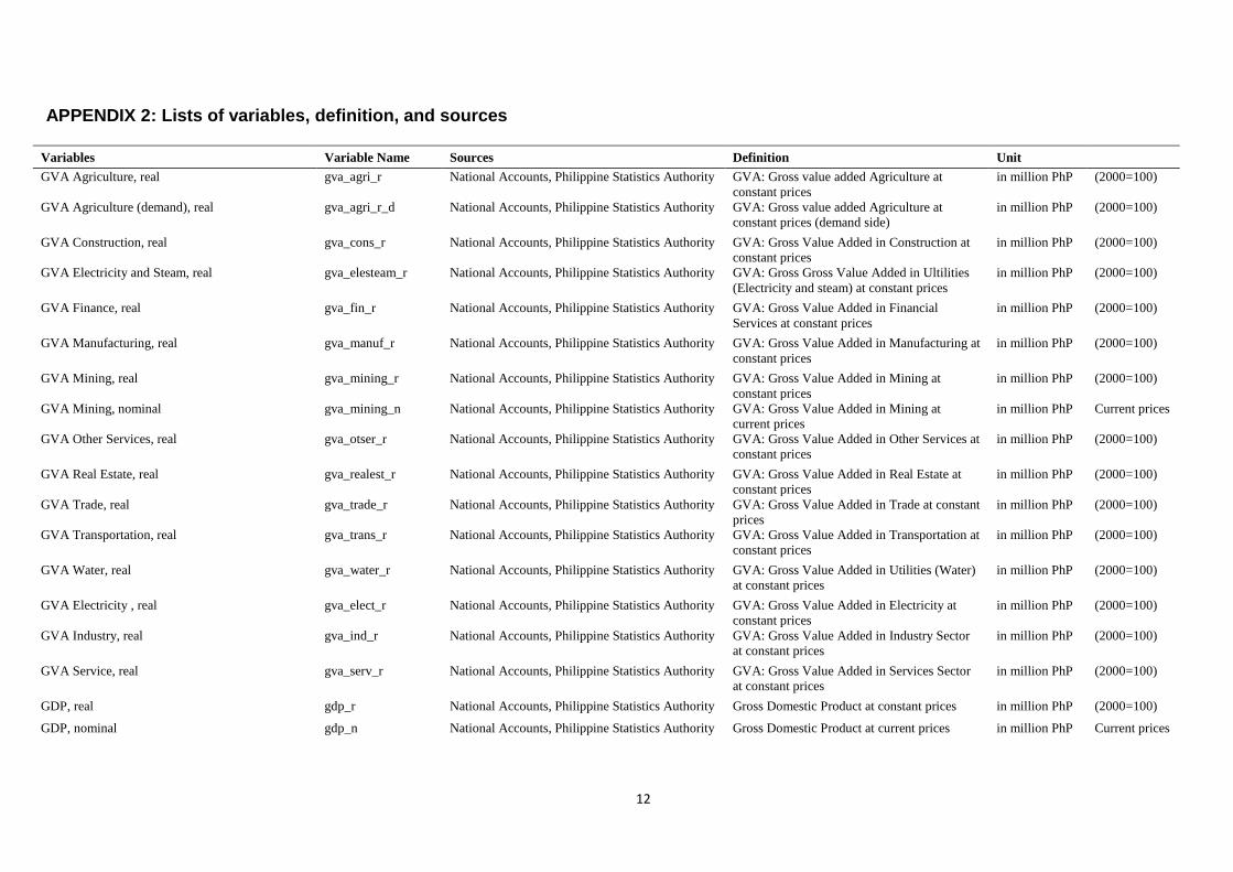
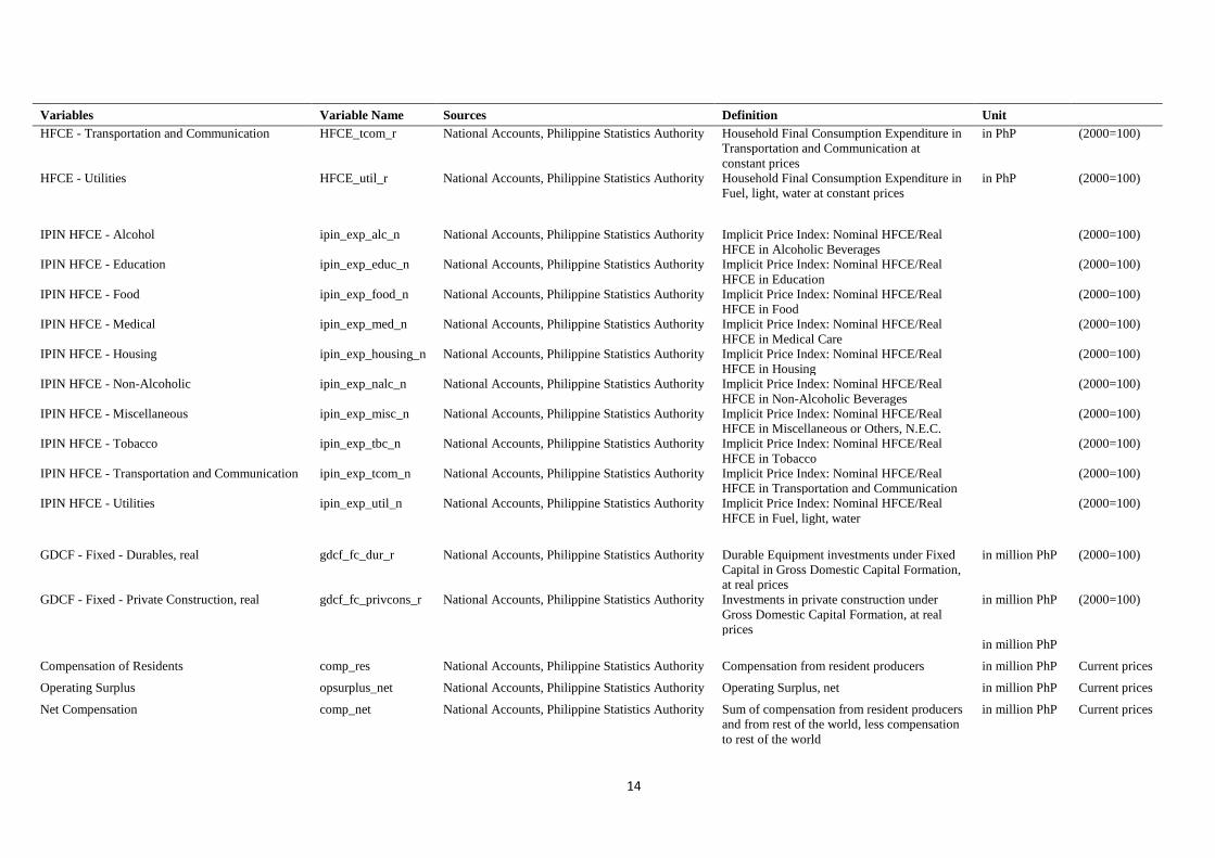
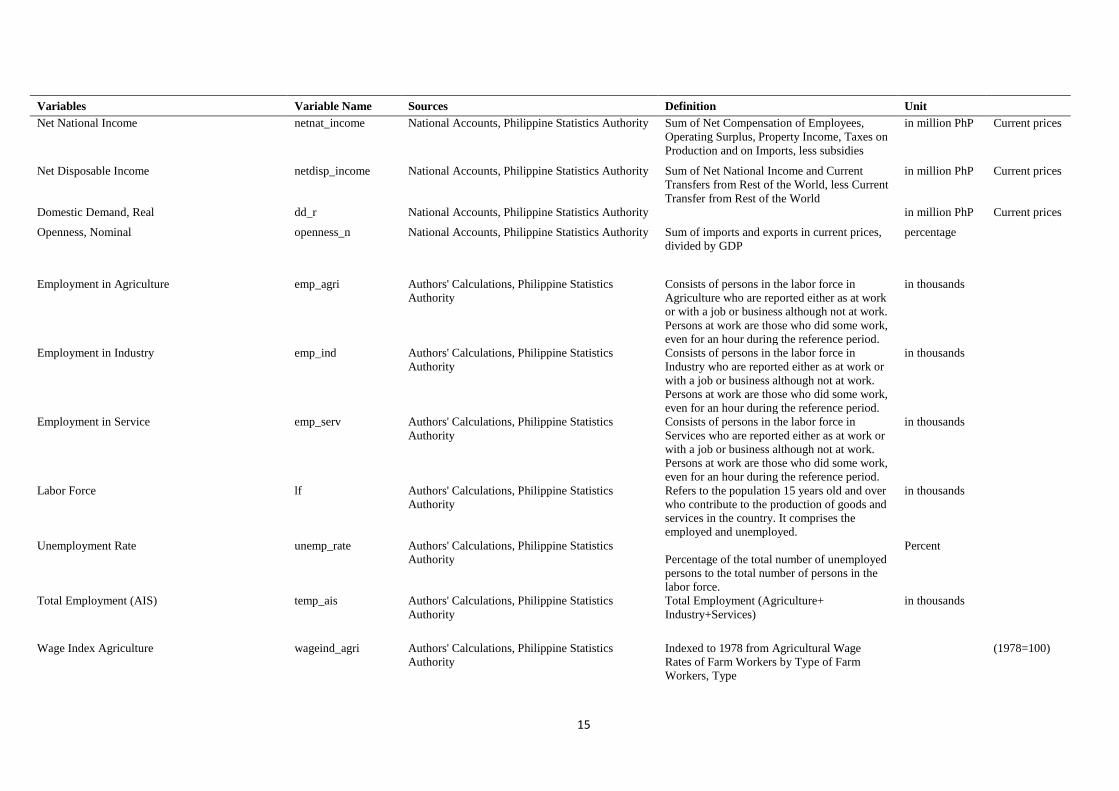
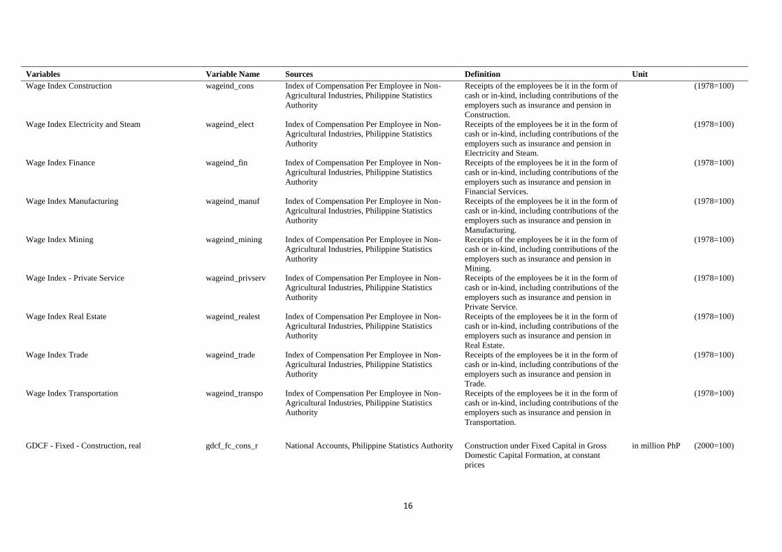
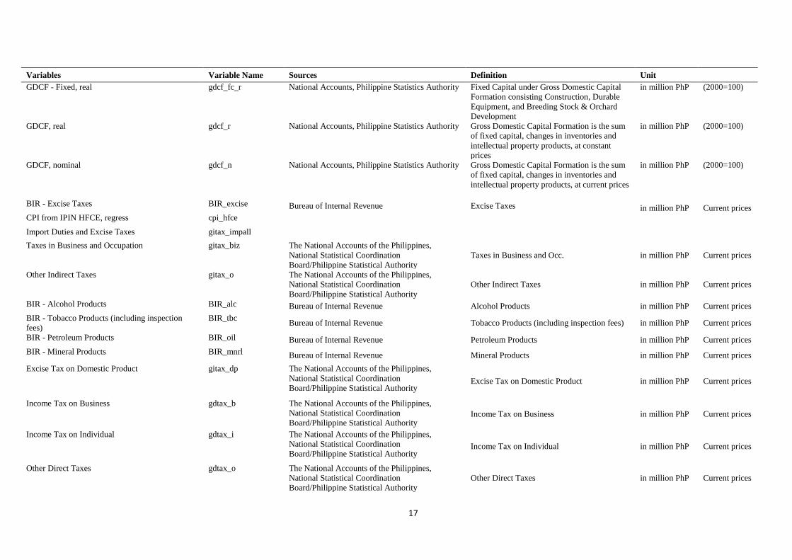
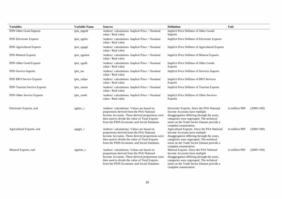
APPENDIX 2: Lists of variables, definition, and sources
Variables Variable Name Sources Definition Unit
GVA Agriculture, real gva_agri_r National Accounts, Philippine Statistics Authority GVA: Gross value added Agriculture at
constant prices
in million PhP (2000=100)
GVA Agriculture (demand), real gva_agri_r_d National Accounts, Philippine Statistics Authority GVA: Gross value added Agriculture at
constant prices (demand side)
in million PhP (2000=100)
GVA Construction, real gva_cons_r National Accounts, Philippine Statistics Authority GVA: Gross Value Added in Construction at
constant prices
in million PhP (2000=100)
GVA Electricity and Steam, real gva_elesteam_r National Accounts, Philippine Statistics Authority GVA: Gross Gross Value Added in Ultilities
(Electricity and steam) at constant prices
in million PhP (2000=100)
GVA Finance, real gva_fin_r National Accounts, Philippine Statistics Authority GVA: Gross Value Added in Financial
Services at constant prices
in million PhP (2000=100)
GVA Manufacturing, real gva_manuf_r National Accounts, Philippine Statistics Authority GVA: Gross Value Added in Manufacturing at
constant prices
in million PhP (2000=100)
GVA Mining, real gva_mining_r National Accounts, Philippine Statistics Authority GVA: Gross Value Added in Mining at
constant prices
in million PhP (2000=100)
GVA Mining, nominal gva_mining_n National Accounts, Philippine Statistics Authority GVA: Gross Value Added in Mining at
current prices
in million PhP Current prices
GVA Other Services, real gva_otser_r National Accounts, Philippine Statistics Authority GVA: Gross Value Added in Other Services at
constant prices
in million PhP (2000=100)
GVA Real Estate, real gva_realest_r National Accounts, Philippine Statistics Authority GVA: Gross Value Added in Real Estate at
constant prices
in million PhP (2000=100)
GVA Trade, real gva_trade_r National Accounts, Philippine Statistics Authority GVA: Gross Value Added in Trade at constant
prices
in million PhP (2000=100)
GVA Transportation, real gva_trans_r National Accounts, Philippine Statistics Authority GVA: Gross Value Added in Transportation at
constant prices
in million PhP (2000=100)
GVA Water, real gva_water_r National Accounts, Philippine Statistics Authority GVA: Gross Value Added in Utilities (Water)
at constant prices
in million PhP (2000=100)
GVA Electricity , real gva_elect_r National Accounts, Philippine Statistics Authority GVA: Gross Value Added in Electricity at
constant prices
in million PhP (2000=100)
GVA Industry, real gva_ind_r National Accounts, Philippine Statistics Authority GVA: Gross Value Added in Industry Sector
at constant prices
in million PhP (2000=100)
GVA Service, real gva_serv_r National Accounts, Philippine Statistics Authority GVA: Gross Value Added in Services Sector
at constant prices
in million PhP (2000=100)
GDP, real gdp_r National Accounts, Philippine Statistics Authority Gross Domestic Product at constant prices in million PhP (2000=100)
GDP, nominal gdp_n National Accounts, Philippine Statistics Authority Gross Domestic Product at current prices in million PhP Current prices

13
Variables Variable Name Sources Definition Unit
IPIN GVA Construction ipin_gva_cons National Accounts, Philippine Statistics Authority Implicit Price Index: Nominal GVA/Real
GVA in Construction
(2000=100)
IPIN GVA Electricity and Steam ipin_gva_elesteam National Accounts, Philippine Statistics Authority Implicit Price Index: Nominal GVA/Real
GVA in Utilities (Electricity and Steam)
(2000=100)
IPIN GVA Finance ipin_gva_fin National Accounts, Philippine Statistics Authority Implicit Price Index: Nominal GVA/Real
GVA in Financial Services
(2000=100)
IPIN GVA Manufacturing ipin_gva_manuf National Accounts, Philippine Statistics Authority Implicit Price Index: Nominal GVA/Real
GVA in Manufacturing
(2000=100)
IPIN GVA Mining ipin_gva_mining National Accounts, Philippine Statistics Authority Implicit Price Index: Nominal GVA/Real
GVA in Mining
(2000=100)
IPIN GVA Other Services ipin_gva_otser National Accounts, Philippine Statistics Authority Implicit Price Index: Nominal GVA/Real
GVA in Other Services
(2000=100)
IPIN GVA Real Estate ipin_gva_realest National Accounts, Philippine Statistics Authority Implicit Price Index: Nominal GVA/Real
GVA in Real Estate
(2000=100)
IPIN GVA Trade ipin_gva_trade National Accounts, Philippine Statistics Authority Implicit Price Index: Nominal GVA/Real
GVA in Trade
(2000=100)
IPIN GVA Transportation ipin_gva_trans National Accounts, Philippine Statistics Authority Implicit Price Index: Nominal GVA/Real
GVA in Transportation
(2000=100)
IPIN GVA Water ipin_gva_water National Accounts, Philippine Statistics Authority Implicit Price Index: Nominal GVA/Real
GVA in Utilities (Water)
(2000=100)
HFCE - Alcohol HFCE_alc_r National Accounts, Philippine Statistics Authority Household Final Consumption Expenditure in
Alcoholic Beverages at constant prices
in PhP (2000=100)
HFCE - Education HFCE_educ_r National Accounts, Philippine Statistics Authority Household Final Consumption Expenditure in
Education at constant prices
in PhP (2000=100)
HFCE - Food HFCE_food_r National Accounts, Philippine Statistics Authority Household Final Consumption Expenditure in
Food at constant prices
in PhP (2000=100)
HFCE - Medical HFCE_med_r National Accounts, Philippine Statistics Authority Household Final Consumption Expenditure in
Medical Care at constant prices
in PhP (2000=100)
HFCE - Housing HFCE_housing_r National Accounts, Philippine Statistics Authority Household Final Consumption Expenditure in
Housing at constant prices
in PhP (2000=100)
HFCE - Non-Alcoholic HFCE_nalc_r National Accounts, Philippine Statistics Authority Household Final Consumption Expenditure in
Non-Alcoholic Beverages at constant prices
in PhP (2000=100)
HFCE - Miscellaneous HFCE_misc_r National Accounts, Philippine Statistics Authority Household Final Consumption Expenditure in
Miscellaneous or Others, N.E.C. at constant
prices
in PhP (2000=100)
HFCE - Tobacco HFCE_tbc_r National Accounts, Philippine Statistics Authority Household Final Consumption Expenditure in
Tobacco at constant prices
in PhP (2000=100)
14
Variables Variable Name Sources Definition Unit
HFCE - Transportation and Communication HFCE_tcom_r National Accounts, Philippine Statistics Authority Household Final Consumption Expenditure in
Transportation and Communication at
constant prices
in PhP (2000=100)
HFCE - Utilities HFCE_util_r National Accounts, Philippine Statistics Authority Household Final Consumption Expenditure in
Fuel, light, water at constant prices
in PhP (2000=100)
IPIN HFCE - Alcohol ipin_exp_alc_n National Accounts, Philippine Statistics Authority Implicit Price Index: Nominal HFCE/Real
HFCE in Alcoholic Beverages
(2000=100)
IPIN HFCE - Education ipin_exp_educ_n National Accounts, Philippine Statistics Authority Implicit Price Index: Nominal HFCE/Real
HFCE in Education
(2000=100)
IPIN HFCE - Food ipin_exp_food_n National Accounts, Philippine Statistics Authority Implicit Price Index: Nominal HFCE/Real
HFCE in Food
(2000=100)
IPIN HFCE - Medical ipin_exp_med_n National Accounts, Philippine Statistics Authority Implicit Price Index: Nominal HFCE/Real
HFCE in Medical Care
(2000=100)
IPIN HFCE - Housing ipin_exp_housing_n National Accounts, Philippine Statistics Authority Implicit Price Index: Nominal HFCE/Real
HFCE in Housing
(2000=100)
IPIN HFCE - Non-Alcoholic ipin_exp_nalc_n National Accounts, Philippine Statistics Authority Implicit Price Index: Nominal HFCE/Real
HFCE in Non-Alcoholic Beverages
(2000=100)
IPIN HFCE - Miscellaneous ipin_exp_misc_n National Accounts, Philippine Statistics Authority Implicit Price Index: Nominal HFCE/Real
HFCE in Miscellaneous or Others, N.E.C.
(2000=100)
IPIN HFCE - Tobacco ipin_exp_tbc_n National Accounts, Philippine Statistics Authority Implicit Price Index: Nominal HFCE/Real
HFCE in Tobacco
(2000=100)
IPIN HFCE - Transportation and Communication ipin_exp_tcom_n National Accounts, Philippine Statistics Authority Implicit Price Index: Nominal HFCE/Real
HFCE in Transportation and Communication
(2000=100)
IPIN HFCE - Utilities ipin_exp_util_n National Accounts, Philippine Statistics Authority Implicit Price Index: Nominal HFCE/Real
HFCE in Fuel, light, water
(2000=100)
GDCF - Fixed - Durables, real gdcf_fc_dur_r National Accounts, Philippine Statistics Authority Durable Equipment investments under Fixed
Capital in Gross Domestic Capital Formation,
at real prices
in million PhP (2000=100)
GDCF - Fixed - Private Construction, real gdcf_fc_privcons_r National Accounts, Philippine Statistics Authority Investments in private construction under
Gross Domestic Capital Formation, at real
prices
in million PhP (2000=100)
in million PhP
Compensation of Residents comp_res National Accounts, Philippine Statistics Authority Compensation from resident producers in million PhP Current prices
Operating Surplus opsurplus_net National Accounts, Philippine Statistics Authority Operating Surplus, net in million PhP Current prices
Net Compensation comp_net National Accounts, Philippine Statistics Authority Sum of compensation from resident producers
and from rest of the world, less compensation
to rest of the world
in million PhP Current prices
15
Variables Variable Name Sources Definition Unit
Net National Income netnat_income National Accounts, Philippine Statistics Authority Sum of Net Compensation of Employees,
Operating Surplus, Property Income, Taxes on
Production and on Imports, less subsidies
in million PhP Current prices
Net Disposable Income netdisp_income National Accounts, Philippine Statistics Authority Sum of Net National Income and Current
Transfers from Rest of the World, less Current
Transfer from Rest of the World
in million PhP Current prices
Domestic Demand, Real dd_r National Accounts, Philippine Statistics Authority
in million PhP Current prices
Openness, Nominal openness_n National Accounts, Philippine Statistics Authority Sum of imports and exports in current prices,
divided by GDP
percentage
Employment in Agriculture emp_agri Authors' Calculations, Philippine Statistics
Authority
Consists of persons in the labor force in
Agriculture who are reported either as at work
or with a job or business although not at work.
Persons at work are those who did some work,
even for an hour during the reference period.
in thousands
Employment in Industry emp_ind Authors' Calculations, Philippine Statistics
Authority
Consists of persons in the labor force in
Industry who are reported either as at work or
with a job or business although not at work.
Persons at work are those who did some work,
even for an hour during the reference period.
in thousands
Employment in Service emp_serv Authors' Calculations, Philippine Statistics
Authority
Consists of persons in the labor force in
Services who are reported either as at work or
with a job or business although not at work.
Persons at work are those who did some work,
even for an hour during the reference period.
in thousands
Labor Force lf Authors' Calculations, Philippine Statistics
Authority
Refers to the population 15 years old and over
who contribute to the production of goods and
services in the country. It comprises the
employed and unemployed.
in thousands
Unemployment Rate unemp_rate Authors' Calculations, Philippine Statistics
Authority
Percentage of the total number of unemployed
persons to the total number of persons in the
labor force.
Percent
Total Employment (AIS) temp_ais Authors' Calculations, Philippine Statistics
Authority
Total Employment (Agriculture+
Industry+Services)
in thousands
Wage Index Agriculture wageind_agri Authors' Calculations, Philippine Statistics
Authority
Indexed to 1978 from Agricultural Wage
Rates of Farm Workers by Type of Farm
Workers, Type
(1978=100)
16
Variables Variable Name Sources Definition Unit
Wage Index Construction wageind_cons Index of Compensation Per Employee in Non-
Agricultural Industries, Philippine Statistics
Authority
Receipts of the employees be it in the form of
cash or in-kind, including contributions of the
employers such as insurance and pension in
Construction.
(1978=100)
Wage Index Electricity and Steam wageind_elect Index of Compensation Per Employee in Non-
Agricultural Industries, Philippine Statistics
Authority
Receipts of the employees be it in the form of
cash or in-kind, including contributions of the
employers such as insurance and pension in
Electricity and Steam.
(1978=100)
Wage Index Finance wageind_fin Index of Compensation Per Employee in Non-
Agricultural Industries, Philippine Statistics
Authority
Receipts of the employees be it in the form of
cash or in-kind, including contributions of the
employers such as insurance and pension in
Financial Services.
(1978=100)
Wage Index Manufacturing wageind_manuf Index of Compensation Per Employee in Non-
Agricultural Industries, Philippine Statistics
Authority
Receipts of the employees be it in the form of
cash or in-kind, including contributions of the
employers such as insurance and pension in
Manufacturing.
(1978=100)
Wage Index Mining wageind_mining Index of Compensation Per Employee in Non-
Agricultural Industries, Philippine Statistics
Authority
Receipts of the employees be it in the form of
cash or in-kind, including contributions of the
employers such as insurance and pension in
Mining.
(1978=100)
Wage Index - Private Service wageind_privserv Index of Compensation Per Employee in Non-
Agricultural Industries, Philippine Statistics
Authority
Receipts of the employees be it in the form of
cash or in-kind, including contributions of the
employers such as insurance and pension in
Private Service.
(1978=100)
Wage Index Real Estate wageind_realest Index of Compensation Per Employee in Non-
Agricultural Industries, Philippine Statistics
Authority
Receipts of the employees be it in the form of
cash or in-kind, including contributions of the
employers such as insurance and pension in
Real Estate.
(1978=100)
Wage Index Trade wageind_trade Index of Compensation Per Employee in Non-
Agricultural Industries, Philippine Statistics
Authority
Receipts of the employees be it in the form of
cash or in-kind, including contributions of the
employers such as insurance and pension in
Trade.
(1978=100)
Wage Index Transportation wageind_transpo Index of Compensation Per Employee in Non-
Agricultural Industries, Philippine Statistics
Authority
Receipts of the employees be it in the form of
cash or in-kind, including contributions of the
employers such as insurance and pension in
Transportation.
(1978=100)
GDCF - Fixed - Construction, real gdcf_fc_cons_r National Accounts, Philippine Statistics Authority Construction under Fixed Capital in Gross
Domestic Capital Formation, at constant
prices
in million PhP (2000=100)
17
Variables Variable Name Sources Definition Unit
GDCF - Fixed, real gdcf_fc_r National Accounts, Philippine Statistics Authority Fixed Capital under Gross Domestic Capital
Formation consisting Construction, Durable
Equipment, and Breeding Stock & Orchard
Development
in million PhP (2000=100)
GDCF, real gdcf_r National Accounts, Philippine Statistics Authority Gross Domestic Capital Formation is the sum
of fixed capital, changes in inventories and
intellectual property products, at constant
prices
in million PhP (2000=100)
GDCF, nominal gdcf_n National Accounts, Philippine Statistics Authority Gross Domestic Capital Formation is the sum
of fixed capital, changes in inventories and
intellectual property products, at current prices
in million PhP (2000=100)
BIR - Excise Taxes BIR_excise Bureau of Internal Revenue Excise Taxes in million PhP Current prices CPI from IPIN HFCE, regress cpi_hfce
Import Duties and Excise Taxes gitax_impall
Taxes in Business and Occupation gitax_biz The National Accounts of the Philippines,
National Statistical Coordination
Board/Philippine Statistical Authority
Taxes in Business and Occ. in million PhP Current prices
Other Indirect Taxes gitax_o The National Accounts of the Philippines,
National Statistical Coordination
Board/Philippine Statistical Authority
Other Indirect Taxes in million PhP Current prices
BIR - Alcohol Products BIR_alc Bureau of Internal Revenue Alcohol Products in million PhP Current prices
BIR - Tobacco Products (including inspection
fees)
BIR_tbc Bureau of Internal Revenue Tobacco Products (including inspection fees) in million PhP Current prices
BIR - Petroleum Products BIR_oil Bureau of Internal Revenue Petroleum Products in million PhP Current prices
BIR - Mineral Products BIR_mnrl Bureau of Internal Revenue Mineral Products in million PhP Current prices
Excise Tax on Domestic Product gitax_dp The National Accounts of the Philippines,
National Statistical Coordination
Board/Philippine Statistical Authority Excise Tax on Domestic Product in million PhP Current prices
Income Tax on Business gdtax_b The National Accounts of the Philippines,
National Statistical Coordination
Board/Philippine Statistical Authority Income Tax on Business in million PhP Current prices
Income Tax on Individual gdtax_i The National Accounts of the Philippines,
National Statistical Coordination
Board/Philippine Statistical Authority Income Tax on Individual in million PhP Current prices
Other Direct Taxes gdtax_o The National Accounts of the Philippines,
National Statistical Coordination
Board/Philippine Statistical Authority
Other Direct Taxes in million PhP Current prices

18
Variables Variable Name Sources Definition Unit
Compulsory fees and fines ggff General Government, Income and Outlay
Account, National Statistical Coordination
Board/Philippine Statistical Authority
Compulsory fees and fines in million PhP Current prices
Govt property income ggproperty General Government, Income and Outlay
Account, National Statistical Coordination
Board/Philippine Statistical Authority
Government property income in million PhP Current prices
Social security contributions ggssc General Government, Income and Outlay
Account, National Statistical Coordination
Board/Philippine Statistical Authority
Social security contributions in million PhP Current prices
Govt property expenditure ggpropexp General Government, Income and Outlay
Account, National Statistical Coordination
Board/Philippine Statistical Authority
Government property expenditure in million PhP Current prices
Social security benefits ggsbenefit General Government, Income and Outlay
Account, National Statistical Coordination
Board/Philippine Statistical Authority
Social security benefits in million PhP Current prices
Implicit Price Index, Government Spending ipin_gfce
Total Indirect Taxes i_tot_indirect_tax
Total Direct Taxes i_tot_direct_tax
Total Taxes i_tot_tax
Total Govt Income i_tot_gov_inc
Total Govt Expenditure i_tot_gov_exp
Total Govt Savings i_tot_govt_sav
Total Govt Surplus i_gov_surp
Total Govt Debt i_gov_debt
IPIN Agricultural Imports ipin_mgagri Authors’ calculations. Implicit Price = Nominal
value / Real value
Implicit Price Deflator of Agricultural Imports Unit
IPIN Fuel Imports ipin_mgfuel Authors’ calculations. Implicit Price = Nominal
value / Real value
Implicit Price Deflator of Fuel Imports
IPIN Machinery Imports ipin_mgmach Authors’ calculations. Implicit Price = Nominal
value / Real value
Implicit Price Deflator of Machinery Imports
IPIN Materials Imports ipin_mgmat Authors’ calculations. Implicit Price = Nominal
value / Real value
Implicit Price Deflator of Materials Imports
19
Variables Variable Name Sources Definition Unit
IPIN Other Good Imports ipin_mgoth Authors’ calculations. Implicit Price = Nominal
value / Real value
Implicit Price Deflator of Other Goods
Imports
IPIN Electronic Exports ipin_xgelec Authors’ calculations. Implicit Price = Nominal
value / Real value
Implicit Price Deflator of Electronic Exports
IPIN Agricultural Exports ipin_xgagri Authors’ calculations. Implicit Price = Nominal
value / Real value
Implicit Price Deflator of Agricultural Exports
IPIN Mineral Exports ipin_xgmine Authors’ calculations. Implicit Price = Nominal
value / Real value
Implicit Price Deflator of Mineral Exports
IPIN Other Good Exports ipin_xgoth Authors’ calculations. Implicit Price = Nominal
value / Real value
Implicit Price Deflator of Other Goods
Exports
IPIN Service Imports ipin_ms Authors’ calculations. Implicit Price = Nominal
value / Real value
Implicit Price Deflator of Services Imports
IPIN BPO Service Exports ipin_xsbpo Authors’ calculations. Implicit Price = Nominal
value / Real value
Implicit Price Deflator of BPO Services
Exports
IPIN Tourism Service Exports ipin_xstour Authors’ calculations. Implicit Price = Nominal
value / Real value
Implicit Price Deflator of Tourism Exports
IPIN Other Service Exports ipin_xsoth Authors’ calculations. Implicit Price = Nominal
value / Real value
Implicit Price Deflator of Other Services
Exports
Electronic Exports, real xgelec_r Authors’ calculations. Values are based on
proportions derived from the PSA National
Income Accounts. These derived proportions were
then used to divide the value of Total Exports
from the PIDS-Economic and Social Database.
Electronic Exports. Since the PSA National
Income Accounts have multiple
disaggregation differing through the years,
categories were regrouped. The technical
notes on the Trade Sector Dataset provide a
complete enumeration.
in million PhP (2000=100)
Agricultural Exports, real xgagri_r Authors’ calculations. Values are based on
proportions derived from the PSA National
Income Accounts. These derived proportions were
then used to divide the value of Total Exports
from the PIDS-Economic and Social Database.
Agricultural Exports. Since the PSA National
Income Accounts have multiple
disaggregation differing through the years,
categories were regrouped. The technical
notes on the Trade Sector Dataset provide a
complete enumeration.
in million PhP (2000=100)
Mineral Exports, real xgmine_r Authors’ calculations. Values are based on
proportions derived from the PSA National
Income Accounts. These derived proportions were
then used to divide the value of Total Exports
from the PIDS-Economic and Social Database.
Mineral Exports. Since the PSA National
Income Accounts have multiple
disaggregation differing through the years,
categories were regrouped. The technical
notes on the Trade Sector Dataset provide a
complete enumeration.
in million PhP (2000=100)

20
Variables Variable Name Sources Definition Unit
Other Good Exports, real xgoth_r Authors’ calculations. Values are based on
proportions derived from the PSA National
Income Accounts. These derived proportions were
then used to divide the value of Total Exports
from the PIDS-Economic and Social Database.
Other Goods Exports. Since the PSA National
Income Accounts have multiple
disaggregation differing through the years,
categories were regrouped. The technical
notes on the Trade Sector Dataset provide a
complete enumeration.
in million PhP (2000=100)
BPO Service Exports, real xsbpo_r Authors’ calculations. Values are based on
proportions derived from the PSA National
Income Accounts. These derived proportions were
then used to divide the value of Total Exports
from the PIDS-Economic and Social Database.
BPO Services Exports. Since the PSA
National Income Accounts have multiple
disaggregation differing through the years,
categories were regrouped. The technical
notes on the Trade Sector Dataset provide a
complete enumeration.
in million PhP (2000=100)
Tourism Service Exports, real xstour_r Authors’ calculations. Values are based on
proportions derived from the PSA National
Income Accounts. These derived proportions were
then used to divide the value of Total Exports
from the PIDS-Economic and Social Database.
Tourism Services Exports. Since the PSA
National Income Accounts have multiple
disaggregation differing through the years,
categories were regrouped. The technical
notes on the Trade Sector Dataset provide a
complete enumeration.
in million PhP (2000=100)
Other Service Exports xsoth_r Authors’ calculations. Values are based on
proportions derived from the PSA National
Income Accounts. These derived proportions were
then used to divide the value of Total Exports
from the PIDS-Economic and Social Database.
Other Services Exports. Since the PSA
National Income Accounts have multiple
disaggregation differing through the years,
categories were regrouped. The technical
notes on the Trade Sector Dataset provide a
complete enumeration.
in million PhP (2000=100)
BOP - Total Good Exports, nominal bopxg_n Bangko Sentral ng Pilipinas Total Goods Exports, Credit in million US$ Current prices
BOP - Total Service Exports, nominal bopxs_n Bangko Sentral ng Pilipinas Total Services Exports, Credit in million US$ Current prices
Agricultural Imports, real mgagri_r Authors’ calculations. Values are based on
proportions derived from the PSA National
Income Accounts. These derived proportions were
then used to divide the value of Total Imports
from the PIDS-Economic and Social Database.
Agricultural Imports. Since the PSA National
Income Accounts have multiple
disaggregation differing through the years,
categories were regrouped. The technical
notes on the Trade Sector Dataset provide a
complete enumeration.
in million PhP (2000=100)
Fuel Imports, real mgfuel_r Authors’ calculations. Values are based on
proportions derived from the PSA National
Income Accounts. These derived proportions were
then used to divide the value of Total Imports
from the PIDS-Economic and Social Database.
Fuel Imports. Since the PSA National Income
Accounts have multiple disaggregation
differing through the years, categories were
regrouped. The technical notes on the Trade
Sector Dataset provide a complete
enumeration.
in million PhP (2000=100)
21
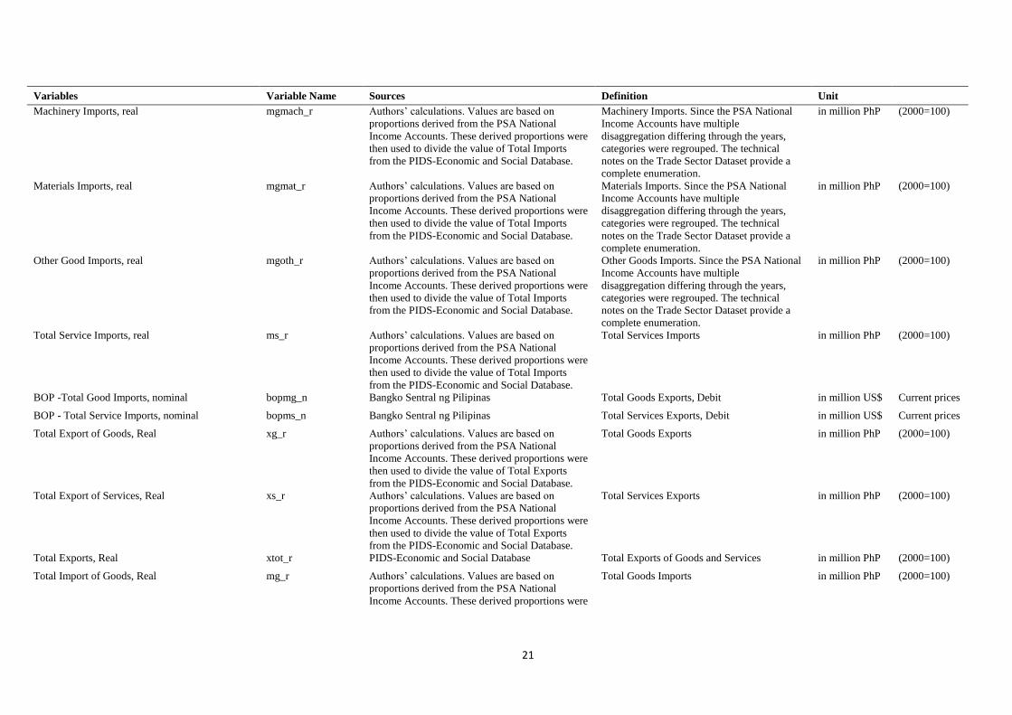
Variables Variable Name Sources Definition Unit
Machinery Imports, real mgmach_r Authors’ calculations. Values are based on
proportions derived from the PSA National
Income Accounts. These derived proportions were
then used to divide the value of Total Imports
from the PIDS-Economic and Social Database.
Machinery Imports. Since the PSA National
Income Accounts have multiple
disaggregation differing through the years,
categories were regrouped. The technical
notes on the Trade Sector Dataset provide a
complete enumeration.
in million PhP (2000=100)
Materials Imports, real mgmat_r Authors’ calculations. Values are based on
proportions derived from the PSA National
Income Accounts. These derived proportions were
then used to divide the value of Total Imports
from the PIDS-Economic and Social Database.
Materials Imports. Since the PSA National
Income Accounts have multiple
disaggregation differing through the years,
categories were regrouped. The technical
notes on the Trade Sector Dataset provide a
complete enumeration.
in million PhP (2000=100)
Other Good Imports, real mgoth_r Authors’ calculations. Values are based on
proportions derived from the PSA National
Income Accounts. These derived proportions were
then used to divide the value of Total Imports
from the PIDS-Economic and Social Database.
Other Goods Imports. Since the PSA National
Income Accounts have multiple
disaggregation differing through the years,
categories were regrouped. The technical
notes on the Trade Sector Dataset provide a
complete enumeration.
in million PhP (2000=100)
Total Service Imports, real ms_r Authors’ calculations. Values are based on
proportions derived from the PSA National
Income Accounts. These derived proportions were
then used to divide the value of Total Imports
from the PIDS-Economic and Social Database.
Total Services Imports in million PhP (2000=100)
BOP -Total Good Imports, nominal bopmg_n Bangko Sentral ng Pilipinas Total Goods Exports, Debit in million US$ Current prices
BOP - Total Service Imports, nominal bopms_n Bangko Sentral ng Pilipinas Total Services Exports, Debit in million US$ Current prices
Total Export of Goods, Real xg_r Authors’ calculations. Values are based on
proportions derived from the PSA National
Income Accounts. These derived proportions were
then used to divide the value of Total Exports
from the PIDS-Economic and Social Database.
Total Goods Exports in million PhP (2000=100)
Total Export of Services, Real xs_r Authors’ calculations. Values are based on
proportions derived from the PSA National
Income Accounts. These derived proportions were
then used to divide the value of Total Exports
from the PIDS-Economic and Social Database.
Total Services Exports in million PhP (2000=100)
Total Exports, Real xtot_r PIDS-Economic and Social Database Total Exports of Goods and Services in million PhP (2000=100)
Total Import of Goods, Real mg_r Authors’ calculations. Values are based on
proportions derived from the PSA National
Income Accounts. These derived proportions were
Total Goods Imports in million PhP (2000=100)

22
Variables Variable Name Sources Definition Unit
then used to divide the value of Total Imports
from the PIDS-Economic and Social Database.
Total Imports, Real mtot_r PIDS-Economic and Social Database Total Imports of Goods and Services in million PhP (2000=100)
Total Imports, Nominal mtot_n PIDS-Economic and Social Database Total Imports of Goods and Services in million PhP Current prices
Net Exports(real) netx_tot
M1 narrowmoney Bangko Sentral ng Pilipinas Consists of currency in circulation (or
currency outside depository corporations) and
peso demand deposits.
in million PhP
M3 broadmoney Bangko Sentral ng Pilipinas Consists of M2 plus peso deposit substitutes,
such as promissory notes and commercial
papers (i.e., securities other than shares
included in broad money)
in million PhP
Total Loans loans Bangko Sentral ng Pilipinas
Resources of the Financial System fsresources Bangko Sentral ng Pilipinas Excludes the Bangko Sentral ng Pilipinas;
amount includes allowance for probable
losses. Includes Investment Houses, Finance
Companies, Investment Companies, Securities
Dealers/Brokers, Pawnshops, Lending
Investors, Non Stocks Savings and Loan
Associations, Credit Card Companies (which
are under BSP supervision), and Private and
Government Insurance Companies (i.e., SSS
and GSIS).
in billion PhP
Cash Remittances cashremit Bangko Sentral ng Pilipinas Overseas Filipinos' Cash Remittances In Thousand
US$
Money Multiplier mm
Inflation* (actual forecast) Inf_hfce_all
23
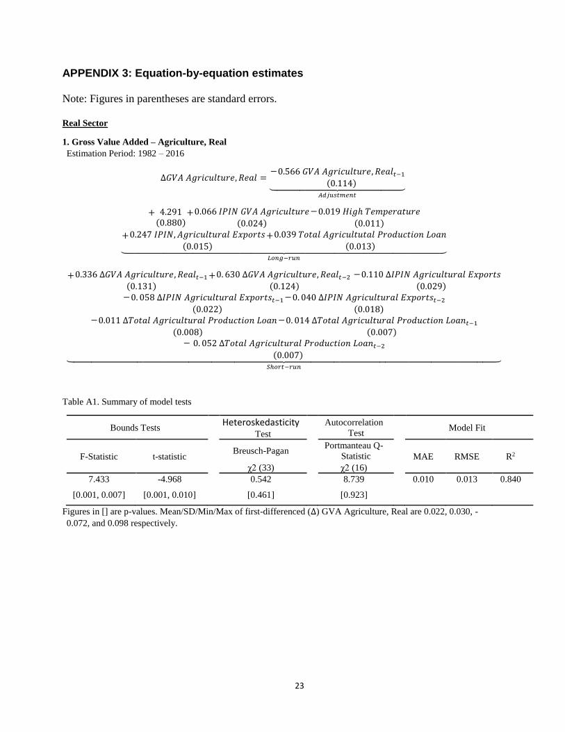
APPENDIX 3: Equation-by-equation estimates
Note: Figures in parentheses are standard errors.
Real Sector
1. Gross Value Added – Agriculture, Real
Estimation Period: 1982 – 2016
∆𝐺𝑉𝐴 𝐴𝑔𝑟𝑖𝑐𝑢𝑙𝑡𝑢𝑟𝑒, 𝑅𝑒𝑎𝑙 =−0.566 𝐺𝑉𝐴 𝐴𝑔𝑟𝑖𝑐𝑢𝑙𝑡𝑢𝑟𝑒, 𝑅𝑒𝑎𝑙𝑡−1
(0.114)⏟ 𝐴𝑑𝑗𝑢𝑠𝑡𝑚𝑒𝑛𝑡
+ 4.291(0.880)
+0.066 𝐼𝑃𝐼𝑁 𝐺𝑉𝐴 𝐴𝑔𝑟𝑖𝑐𝑢𝑙𝑡𝑢𝑟𝑒
(0.024)
−0.019 𝐻𝑖𝑔ℎ 𝑇𝑒𝑚𝑝𝑒𝑟𝑎𝑡𝑢𝑟𝑒
(0.011)
+0.247 𝐼𝑃𝐼𝑁, 𝐴𝑔𝑟𝑖𝑐𝑢𝑙𝑡𝑢𝑟𝑎𝑙 𝐸𝑥𝑝𝑜𝑟𝑡𝑠
(0.015)+0.039 𝑇𝑜𝑡𝑎𝑙 𝐴𝑔𝑟𝑖𝑐𝑢𝑙𝑡𝑢𝑡𝑎𝑙 𝑃𝑟𝑜𝑑𝑢𝑐𝑡𝑖𝑜𝑛 𝐿𝑜𝑎𝑛
(0.013)⏟ 𝐿𝑜𝑛𝑔−𝑟𝑢𝑛
+0.336 ∆𝐺𝑉𝐴 𝐴𝑔𝑟𝑖𝑐𝑢𝑙𝑡𝑢𝑟𝑒, 𝑅𝑒𝑎𝑙𝑡−1(0.131)
+0. 630 ∆𝐺𝑉𝐴 𝐴𝑔𝑟𝑖𝑐𝑢𝑙𝑡𝑢𝑟𝑒, 𝑅𝑒𝑎𝑙𝑡−2
(0.124)
−0.110 ∆𝐼𝑃𝐼𝑁 𝐴𝑔𝑟𝑖𝑐𝑢𝑙𝑡𝑢𝑟𝑎𝑙 𝐸𝑥𝑝𝑜𝑟𝑡𝑠
(0.029)−0. 058 ∆𝐼𝑃𝐼𝑁 𝐴𝑔𝑟𝑖𝑐𝑢𝑙𝑡𝑢𝑟𝑎𝑙 𝐸𝑥𝑝𝑜𝑟𝑡𝑠𝑡−1
(0.022)
−0. 040 ∆𝐼𝑃𝐼𝑁 𝐴𝑔𝑟𝑖𝑐𝑢𝑙𝑡𝑢𝑟𝑎𝑙 𝐸𝑥𝑝𝑜𝑟𝑡𝑠𝑡−2(0.018)
−0.011 ∆𝑇𝑜𝑡𝑎𝑙 𝐴𝑔𝑟𝑖𝑐𝑢𝑙𝑡𝑢𝑟𝑎𝑙 𝑃𝑟𝑜𝑑𝑢𝑐𝑡𝑖𝑜𝑛 𝐿𝑜𝑎𝑛
(0.008)
−0. 014 ∆𝑇𝑜𝑡𝑎𝑙 𝐴𝑔𝑟𝑖𝑐𝑢𝑙𝑡𝑢𝑟𝑎𝑙 𝑃𝑟𝑜𝑑𝑢𝑐𝑡𝑖𝑜𝑛 𝐿𝑜𝑎𝑛𝑡−1(0.007)
− 0. 052 ∆𝑇𝑜𝑡𝑎𝑙 𝐴𝑔𝑟𝑖𝑐𝑢𝑙𝑡𝑢𝑟𝑎𝑙 𝑃𝑟𝑜𝑑𝑢𝑐𝑡𝑖𝑜𝑛 𝐿𝑜𝑎𝑛𝑡−2(0.007)⏟
𝑆ℎ𝑜𝑟𝑡−𝑟𝑢𝑛
Table A1. Summary of model tests
Bounds Tests Heteroskedasticity
Test Autocorrelation
Test Model Fit
F-Statistic t-statistic Breusch-Pagan Portmanteau Q-
Statistic MAE RMSE R2
χ2 (33) χ2 (16)
7.433 -4.968 0.542 8.739 0.010 0.013 0.840
[0.001, 0.007] [0.001, 0.010] [0.461] [0.923]
Figures in [] are p-values. Mean/SD/Min/Max of first-differenced (∆) GVA Agriculture, Real are 0.022, 0.030, -
0.072, and 0.098 respectively.

24
Figure 1. Actual v. Predicted GVA Agriculture, Real, along with residuals
Panel A: Log first-difference Panel B: Log level
Panel C: Model Residuals Panel D: Autocorrelation of Residuals
2. Gross Value Added – Agriculture (Demand), Real
Estimation Period: 1971 – 2016
∆𝐺𝑉𝐴 𝐴𝑔𝑟𝑖𝑐𝑢𝑙𝑡𝑢𝑟𝑒 (𝐷𝑒𝑚𝑎𝑛𝑑), 𝑅𝑒𝑎𝑙 =−0.266 𝐺𝑉𝐴 𝐴𝑔𝑟𝑖𝑐𝑢𝑙𝑡𝑢𝑟𝑒 (𝐷𝑒𝑚𝑎𝑛𝑑), 𝑅𝑒𝑎𝑙𝑡−1
(0.075)⏟ 𝐴𝑑𝑗𝑢𝑠𝑡𝑚𝑒𝑛𝑡
+ 1.418(0.495)
−0.218 𝐼𝑃𝐼𝑁 𝐺𝑉𝐴 𝐴𝑔𝑟𝑖𝑐𝑢𝑙𝑡𝑢𝑟𝑒
(0.083)
+0.306 𝐶𝑜𝑚𝑝𝑒𝑛𝑠𝑎𝑡𝑖𝑜𝑛 𝑜𝑓 𝑅𝑒𝑠𝑖𝑑𝑒𝑛𝑡𝑠
(0.059)+0.094 𝑅𝑒𝑎𝑙 𝐸𝑓𝑓𝑒𝑐𝑡𝑖𝑣𝑒 𝐸𝑥𝑐ℎ𝑎𝑛𝑔𝑒 𝑅𝑎𝑡𝑒
(0.089)⏟ 𝐿𝑜𝑛𝑔−𝑟𝑢𝑛
−0.108 ∆𝐶𝑜𝑚𝑝𝑒𝑛𝑠𝑎𝑡𝑖𝑜𝑛 𝑜𝑓 𝑅𝑒𝑠𝑖𝑑𝑒𝑛𝑡𝑠
(0.043)
−0.162 ∆𝐶𝑜𝑚𝑝𝑒𝑛𝑠𝑎𝑡𝑖𝑜𝑛 𝑜𝑓 𝑅𝑒𝑠𝑖𝑑𝑒𝑛𝑡𝑠𝑡−1(0.044)
−0.101 ∆𝑅𝑒𝑎𝑙 𝐸𝑓𝑓𝑒𝑐𝑡𝑖𝑣𝑒 𝐸𝑥𝑐ℎ𝑎𝑛𝑔𝑒 𝑅𝑎𝑡𝑒
(0.031)
−0.054 ∆𝑅𝑒𝑎𝑙 𝐸𝑓𝑓𝑒𝑐𝑡𝑖𝑣𝑒 𝐸𝑥𝑐ℎ𝑎𝑛𝑔𝑒 𝑅𝑎𝑡𝑒𝑡−1(0.027)⏟
𝑆ℎ𝑜𝑟𝑡−𝑟𝑢𝑛
25
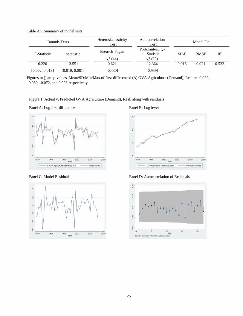
Table A1. Summary of model tests
Bounds Tests Heteroskedasticity
Test Autocorrelation
Test Model Fit
F-Statistic t-statistic Breusch-Pagan Portmanteau Q-
Statistic MAE RMSE R2
χ2 (44) χ2 (22)
6.220 -3.551 0.621 12.364 0.016 0.021 0.522
[0.002, 0.013] [0.010, 0.081] [0.430] [0.949]
Figures in [] are p-values. Mean/SD/Min/Max of first-differenced (∆) GVA Agriculture (Demand), Real are 0.022,
0.030, -0.072, and 0.098 respectively.
Figure 1. Actual v. Predicted GVA Agriculture (Demand), Real, along with residuals
Panel A: Log first-difference Panel B: Log level
Panel C: Model Residuals Panel D: Autocorrelation of Residuals
26
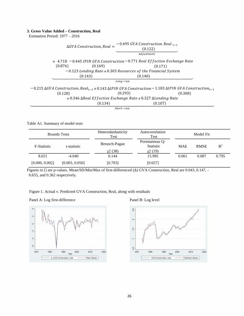
3. Gross Value Added – Construction, Real
Estimation Period: 1977 – 2016
∆𝐺𝑉𝐴 𝐶𝑜𝑛𝑠𝑡𝑟𝑢𝑐𝑡𝑖𝑜𝑛, 𝑅𝑒𝑎𝑙 =−0.495 𝐺𝑉𝐴 𝐶𝑜𝑛𝑠𝑡𝑟𝑢𝑐𝑡𝑖𝑜𝑛. 𝑅𝑒𝑎𝑙 𝑡−1
(0.122)⏟ 𝐴𝑑𝑗𝑢𝑠𝑡𝑚𝑒𝑛𝑡
+ 4.718(0.876)
−0.445 𝐼𝑃𝐼𝑁 𝐺𝑉𝐴 𝐶𝑜𝑛𝑠𝑡𝑟𝑢𝑐𝑡𝑖𝑜𝑛(0.169)
−0.771 𝑅𝑒𝑎𝑙 𝐸𝑓𝑓𝑒𝑐𝑡𝑖𝑣𝑒 𝐸𝑥𝑐ℎ𝑎𝑛𝑔𝑒 𝑅𝑎𝑡𝑒
(0.171)−0.123 𝐿𝑒𝑛𝑑𝑖𝑛𝑔 𝑅𝑎𝑡𝑒
(0.143)+0.303 𝑅𝑒𝑠𝑜𝑢𝑟𝑐𝑒𝑠 𝑜𝑓 𝑡ℎ𝑒 𝐹𝑖𝑛𝑎𝑛𝑐𝑖𝑎𝑙 𝑆𝑦𝑠𝑡𝑒𝑚
(0.140)⏟ 𝐿𝑜𝑛𝑔−𝑟𝑢𝑛
−0.215 ∆𝐺𝑉𝐴 𝐶𝑜𝑛𝑠𝑡𝑟𝑢𝑐𝑡𝑖𝑜𝑛, 𝑅𝑒𝑎𝑙𝑡−1(0.128)
+0.143 ∆𝐼𝑃𝐼𝑁 𝐺𝑉𝐴 𝐶𝑜𝑛𝑠𝑡𝑟𝑢𝑐𝑡𝑖𝑜𝑛(0.293)
−1.183 ∆𝐼𝑃𝐼𝑁 𝐺𝑉𝐴 𝐶𝑜𝑛𝑠𝑡𝑟𝑢𝑐𝑡𝑖𝑜𝑛𝑡−1(0.308)
+0.346 ∆𝑅𝑒𝑎𝑙 𝐸𝑓𝑓𝑒𝑐𝑡𝑖𝑣𝑒 𝐸𝑥𝑐ℎ𝑎𝑛𝑔𝑒 𝑅𝑎𝑡𝑒
(0.134)+0.327 ∆𝐿𝑒𝑛𝑑𝑖𝑛𝑔 𝑅𝑎𝑡𝑒
(0.107)⏟ 𝑆ℎ𝑜𝑟𝑡−𝑟𝑢𝑛
Table A1. Summary of model tests
Bounds Tests Heteroskedasticity
Test Autocorrelation
Test Model Fit
F-Statistic t-statistic Breusch-Pagan Portmanteau Q-
Statistic MAE RMSE R2
χ2 (38) χ2 (19)
8.021 -4.040 0.144 15.995 0.061 0.087 0.795
[0.000, 0.002] [0.003, 0.050] [0.703] [0.657]
Figures in [] are p-values. Mean/SD/Min/Max of first-differenced (∆) GVA Construction, Real are 0.043, 0.147, -
0.655, and 0.362 respectively.
Figure 1. Actual v. Predicted GVA Construction, Real, along with residuals
Panel A: Log first-difference Panel B: Log level
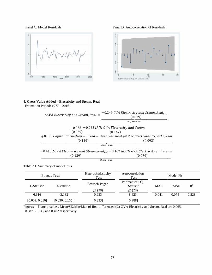
27
Panel C: Model Residuals Panel D: Autocorrelation of Residuals
4. Gross Value Added – Electricity and Steam, Real
Estimation Period: 1977 – 2016
∆𝐺𝑉𝐴 𝐸𝑙𝑒𝑐𝑡𝑟𝑖𝑐𝑖𝑡𝑦 𝑎𝑛𝑑 𝑆𝑡𝑒𝑎𝑚, 𝑅𝑒𝑎𝑙 =−0.249 𝐺𝑉𝐴 𝐸𝑙𝑒𝑐𝑡𝑟𝑖𝑐𝑖𝑡𝑦 𝑎𝑛𝑑 𝑆𝑡𝑒𝑎𝑚, 𝑅𝑒𝑎𝑙𝑡−1
(0.079)⏟ 𝐴𝑑𝑗𝑢𝑠𝑡𝑚𝑒𝑛𝑡
+ 0.055(0.239)
−0.083 𝐼𝑃𝐼𝑁 𝐺𝑉𝐴 𝐸𝑙𝑒𝑐𝑡𝑟𝑖𝑐𝑖𝑡𝑦 𝑎𝑛𝑑 𝑆𝑡𝑒𝑎𝑚(0.147)
+0.533 𝐶𝑎𝑝𝑖𝑡𝑎𝑙 𝐹𝑜𝑟𝑚𝑎𝑡𝑖𝑜𝑛 − 𝐹𝑖𝑥𝑒𝑑 − 𝐷𝑢𝑟𝑎𝑏𝑙𝑒𝑠, 𝑅𝑒𝑎𝑙(0.149)
+0.232 𝐸𝑙𝑒𝑐𝑡𝑟𝑜𝑛𝑖𝑐 𝐸𝑥𝑝𝑜𝑟𝑡𝑠, 𝑅𝑒𝑎𝑙(0.093)⏟
𝐿𝑜𝑛𝑔−𝑟𝑢𝑛
−0.410 ∆𝐺𝑉𝐴 𝐸𝑙𝑒𝑐𝑡𝑟𝑖𝑐𝑖𝑡𝑦 𝑎𝑛𝑑 𝑆𝑡𝑒𝑎𝑚, 𝑅𝑒𝑎𝑙𝑡−1(0.129)
−0.167 ∆𝐼𝑃𝐼𝑁 𝐺𝑉𝐴 𝐸𝑙𝑒𝑐𝑡𝑟𝑖𝑐𝑖𝑡𝑦 𝑠𝑛𝑑 𝑆𝑡𝑒𝑎𝑚(0.079)⏟
𝑆ℎ𝑜𝑟𝑡−𝑟𝑢𝑛
Table A1. Summary of model tests
Bounds Tests Heteroskedasticity
Test Autocorrelation
Test Model Fit
F-Statistic t-statistic Breusch-Pagan Portmanteau Q-
Statistic MAE RMSE R2
χ2 (38) χ2 (20)
6.616 -3.132 0.933 8.423 0.041 0.074 0.528
[0.002, 0.010] [0.030, 0.165] [0.333] [0.988]
Figures in [] are p-values. Mean/SD/Min/Max of first-differenced (∆) GVA Electricity and Steam, Real are 0.065,
0.087, -0.136, and 0.482 respectively.
28
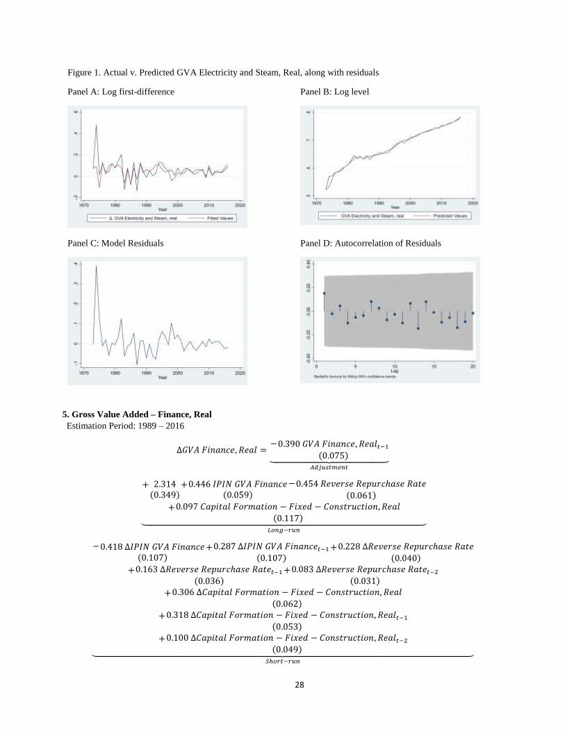
Figure 1. Actual v. Predicted GVA Electricity and Steam, Real, along with residuals
Panel A: Log first-difference Panel B: Log level
Panel C: Model Residuals Panel D: Autocorrelation of Residuals
5. Gross Value Added – Finance, Real
Estimation Period: 1989 – 2016
∆𝐺𝑉𝐴 𝐹𝑖𝑛𝑎𝑛𝑐𝑒, 𝑅𝑒𝑎𝑙 =−0.390 𝐺𝑉𝐴 𝐹𝑖𝑛𝑎𝑛𝑐𝑒, 𝑅𝑒𝑎𝑙𝑡−1
(0.075)⏟ 𝐴𝑑𝑗𝑢𝑠𝑡𝑚𝑒𝑛𝑡
+ 2.314(0.349)
+0.446 𝐼𝑃𝐼𝑁 𝐺𝑉𝐴 𝐹𝑖𝑛𝑎𝑛𝑐𝑒(0.059)
−0.454 𝑅𝑒𝑣𝑒𝑟𝑠𝑒 𝑅𝑒𝑝𝑢𝑟𝑐ℎ𝑎𝑠𝑒 𝑅𝑎𝑡𝑒(0.061)
+0.097 𝐶𝑎𝑝𝑖𝑡𝑎𝑙 𝐹𝑜𝑟𝑚𝑎𝑡𝑖𝑜𝑛 − 𝐹𝑖𝑥𝑒𝑑 − 𝐶𝑜𝑛𝑠𝑡𝑟𝑢𝑐𝑡𝑖𝑜𝑛, 𝑅𝑒𝑎𝑙(0.117)⏟
𝐿𝑜𝑛𝑔−𝑟𝑢𝑛
−0.418 ∆𝐼𝑃𝐼𝑁 𝐺𝑉𝐴 𝐹𝑖𝑛𝑎𝑛𝑐𝑒(0.107)
+0.287 ∆𝐼𝑃𝐼𝑁 𝐺𝑉𝐴 𝐹𝑖𝑛𝑎𝑛𝑐𝑒𝑡−1(0.107)
+0.228 ∆𝑅𝑒𝑣𝑒𝑟𝑠𝑒 𝑅𝑒𝑝𝑢𝑟𝑐ℎ𝑎𝑠𝑒 𝑅𝑎𝑡𝑒(0.040)
+0.163 ∆𝑅𝑒𝑣𝑒𝑟𝑠𝑒 𝑅𝑒𝑝𝑢𝑟𝑐ℎ𝑎𝑠𝑒 𝑅𝑎𝑡𝑒𝑡−1(0.036)
+0.083 ∆𝑅𝑒𝑣𝑒𝑟𝑠𝑒 𝑅𝑒𝑝𝑢𝑟𝑐ℎ𝑎𝑠𝑒 𝑅𝑎𝑡𝑒𝑡−2(0.031)
+0.306 ∆𝐶𝑎𝑝𝑖𝑡𝑎𝑙 𝐹𝑜𝑟𝑚𝑎𝑡𝑖𝑜𝑛 − 𝐹𝑖𝑥𝑒𝑑 − 𝐶𝑜𝑛𝑠𝑡𝑟𝑢𝑐𝑡𝑖𝑜𝑛, 𝑅𝑒𝑎𝑙(0.062)
+0.318 ∆𝐶𝑎𝑝𝑖𝑡𝑎𝑙 𝐹𝑜𝑟𝑚𝑎𝑡𝑖𝑜𝑛 − 𝐹𝑖𝑥𝑒𝑑 − 𝐶𝑜𝑛𝑠𝑡𝑟𝑢𝑐𝑡𝑖𝑜𝑛, 𝑅𝑒𝑎𝑙𝑡−1(0.053)
+0.100 ∆𝐶𝑎𝑝𝑖𝑡𝑎𝑙 𝐹𝑜𝑟𝑚𝑎𝑡𝑖𝑜𝑛 − 𝐹𝑖𝑥𝑒𝑑 − 𝐶𝑜𝑛𝑠𝑡𝑟𝑢𝑐𝑡𝑖𝑜𝑛, 𝑅𝑒𝑎𝑙𝑡−2(0.049)⏟
𝑆ℎ𝑜𝑟𝑡−𝑟𝑢𝑛
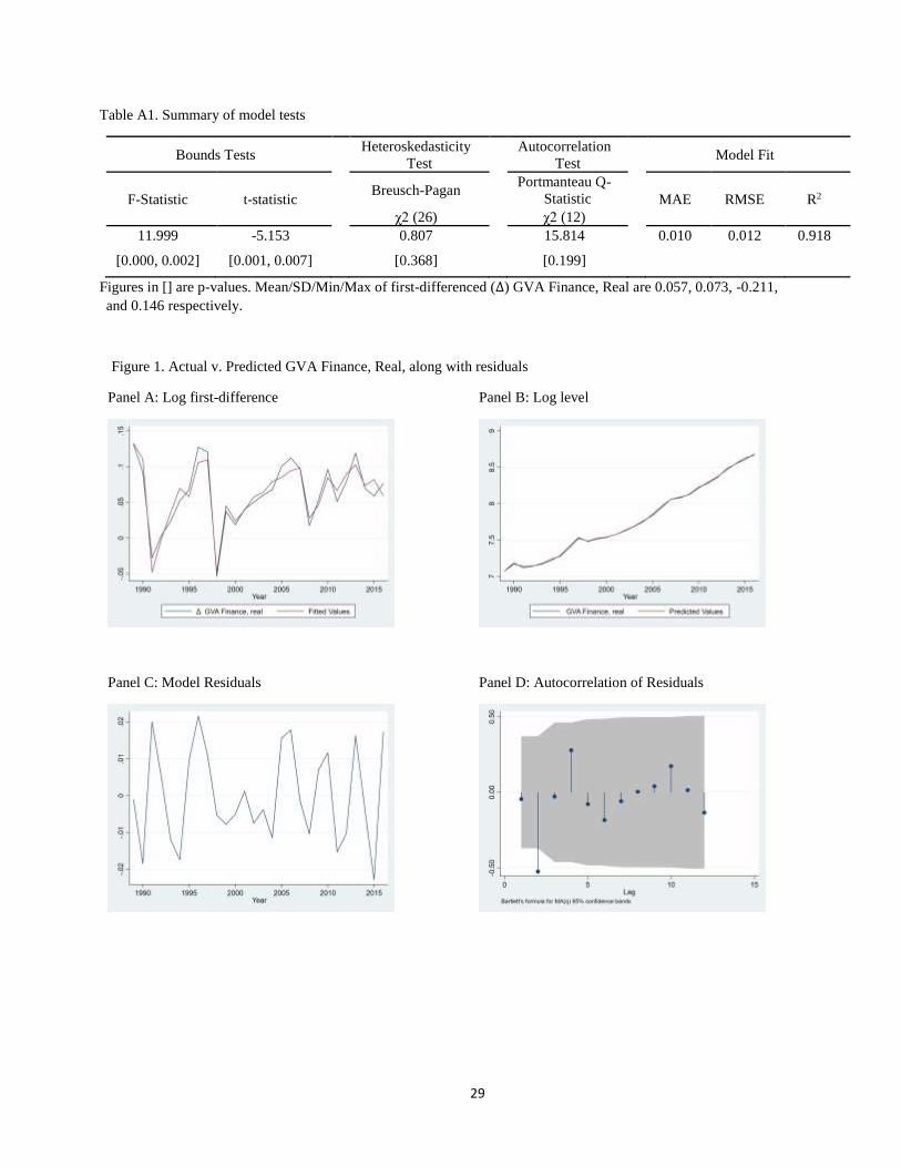
29
Table A1. Summary of model tests
Bounds Tests Heteroskedasticity
Test Autocorrelation
Test Model Fit
F-Statistic t-statistic Breusch-Pagan Portmanteau Q-
Statistic MAE RMSE R2
χ2 (26) χ2 (12)
11.999 -5.153 0.807 15.814 0.010 0.012 0.918
[0.000, 0.002] [0.001, 0.007] [0.368] [0.199]
Figures in [] are p-values. Mean/SD/Min/Max of first-differenced (∆) GVA Finance, Real are 0.057, 0.073, -0.211,
and 0.146 respectively.
Figure 1. Actual v. Predicted GVA Finance, Real, along with residuals
Panel A: Log first-difference Panel B: Log level
Panel C: Model Residuals
Panel D: Autocorrelation of Residuals
30
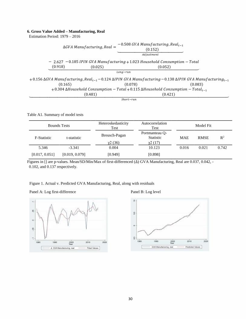
6. Gross Value Added – Manufacturing, Real
Estimation Period: 1979 – 2016
∆𝐺𝑉𝐴 𝑀𝑎𝑛𝑢𝑓𝑎𝑐𝑡𝑢𝑟𝑖𝑛𝑔, 𝑅𝑒𝑎𝑙 =−0.508 𝐺𝑉𝐴 𝑀𝑎𝑛𝑢𝑓𝑎𝑐𝑡𝑢𝑟𝑖𝑛𝑔, 𝑅𝑒𝑎𝑙𝑡−1
(0.152)⏟ 𝐴𝑑𝑗𝑢𝑠𝑡𝑚𝑒𝑛𝑡
− 2.627(0.918)
−0.185 𝐼𝑃𝐼𝑁 𝐺𝑉𝐴 𝑀𝑎𝑛𝑢𝑓𝑎𝑐𝑡𝑢𝑟𝑖𝑛𝑔
(0.025)+1.023 𝐻𝑜𝑢𝑠𝑒ℎ𝑜𝑙𝑑 𝐶𝑜𝑛𝑠𝑢𝑚𝑝𝑡𝑖𝑜𝑛 − 𝑇𝑜𝑡𝑎𝑙
(0.052)⏟ 𝐿𝑜𝑛𝑔−𝑟𝑢𝑛
+0.156 ∆𝐺𝑉𝐴 𝑀𝑎𝑛𝑢𝑓𝑎𝑐𝑡𝑢𝑟𝑖𝑛𝑔, 𝑅𝑒𝑎𝑙𝑡−1(0.165)
−0.124 ∆𝐼𝑃𝐼𝑁 𝐺𝑉𝐴 𝑀𝑎𝑛𝑢𝑓𝑎𝑐𝑡𝑢𝑟𝑖𝑛𝑔
(0.078)
−0.138 ∆𝐼𝑃𝐼𝑁 𝐺𝑉𝐴 𝑀𝑎𝑛𝑢𝑓𝑎𝑐𝑡𝑢𝑟𝑖𝑛𝑔𝑡−1(0.083)
+0.304 ∆𝐻𝑜𝑢𝑠𝑒ℎ𝑜𝑙𝑑 𝐶𝑜𝑛𝑠𝑢𝑚𝑝𝑡𝑖𝑜𝑛 − 𝑇𝑜𝑡𝑎𝑙
(0.481)+0.115 ∆𝐻𝑜𝑢𝑠𝑒ℎ𝑜𝑙𝑑 𝐶𝑜𝑛𝑠𝑢𝑚𝑝𝑡𝑖𝑜𝑛 − 𝑇𝑜𝑡𝑎𝑙𝑡−1
(0.421)⏟ 𝑆ℎ𝑜𝑟𝑡−𝑟𝑢𝑛
Table A1. Summary of model tests
Bounds Tests Heteroskedasticity
Test Autocorrelation
Test Model Fit
F-Statistic t-statistic Breusch-Pagan Portmanteau Q-
Statistic MAE RMSE R2
χ2 (36) χ2 (17)
5.346 -3.341 0.004 10.123 0.016 0.021 0.742
[0.017, 0.051] [0.019, 0.079] [0.949] [0.898]
Figures in [] are p-values. Mean/SD/Min/Max of first-differenced (∆) GVA Manufacturing, Real are 0.037, 0.042, -
0.102, and 0.137 respectively.
Figure 1. Actual v. Predicted GVA Manufacturing, Real, along with residuals
Panel A: Log first-difference Panel B: Log level

31
Panel C: Model Residuals Panel D: Autocorrelation of Residuals
7. Gross Value Added – Mining, Real
Estimation Period: 1990 – 2016
∆𝐺𝑉𝐴 𝑀𝑖𝑛𝑖𝑛𝑔, 𝑅𝑒𝑎𝑙 =−0.919 𝐺𝑉𝐴 𝑀𝑖𝑛𝑖𝑛𝑔, 𝑅𝑒𝑎𝑙𝑡−1
(0.140)⏟ 𝐴𝑑𝑗𝑢𝑠𝑡𝑚𝑒𝑛𝑡
− 10.629(3.038)
−0.226 𝐼𝑃𝐼𝑁 𝐺𝑉𝐴 𝑀𝑖𝑛𝑖𝑛𝑔
(0.152)
−0.538 𝐼𝑃𝐼𝑁 𝐸𝑙𝑒𝑐𝑡𝑟𝑜𝑛𝑖𝑐 𝐸𝑥𝑝𝑜𝑟𝑡𝑠
(0.070)
+0.813 𝑊𝑜𝑟𝑙𝑑 𝐺𝐷𝑃. 𝑅𝑒𝑎𝑙(0.176)
+0.269 𝐺𝑜𝑙𝑑 𝑃𝑟𝑖𝑐𝑒 𝑃𝐻𝑃(0.135)⏟
𝐿𝑜𝑛𝑔−𝑟𝑢𝑛
−0.278 ∆𝐼𝑃𝐼𝑁 𝐺𝑉𝐴 𝑀𝑖𝑛𝑖𝑛𝑔
(0.191)+0.361 ∆𝐼𝑃𝐼𝑁 𝐸𝑙𝑒𝑐𝑡𝑟𝑜𝑛𝑖𝑐 𝐸𝑥𝑝𝑜𝑟𝑡𝑠
(0.138)
−0.358 ∆𝑊𝑜𝑟𝑙𝑑 𝐺𝐷𝑃, 𝑅𝑒𝑎𝑙(0.284)
−0.400 ∆𝑊𝑜𝑟𝑙𝑑 𝐺𝐷𝑃, 𝑅𝑒𝑎𝑙𝑡−1(0.215)
+0.048 ∆𝑊𝑜𝑟𝑙𝑑 𝐺𝐷𝑃, 𝑅𝑒𝑎𝑙𝑡−2(0.208)
−0.574 ∆𝑊𝑜𝑟𝑙𝑑 𝐺𝐷𝑃, 𝑅𝑒𝑎𝑙𝑡−3(0.243)⏟
𝑆ℎ𝑜𝑟𝑡−𝑟𝑢𝑛
Table A1. Summary of model tests
Bounds Tests Heteroskedasticity
Test Autocorrelation
Test Model Fit
F-Statistic t-statistic Breusch-Pagan Portmanteau Q-
Statistic MAE RMSE R2
χ2 (25) χ2 (13)
12.104 -6.552 0.022 12.342 0.071 0.126 0.901
[0.000, 0.001] [0.000, 0.001] [0.880] [0.499]
Figures in [] are p-values. Mean/SD/Min/Max of first-differenced (∆) GVA Mining, Real are 0.037, 0.134, -0.579,
and 0.495 respectively.
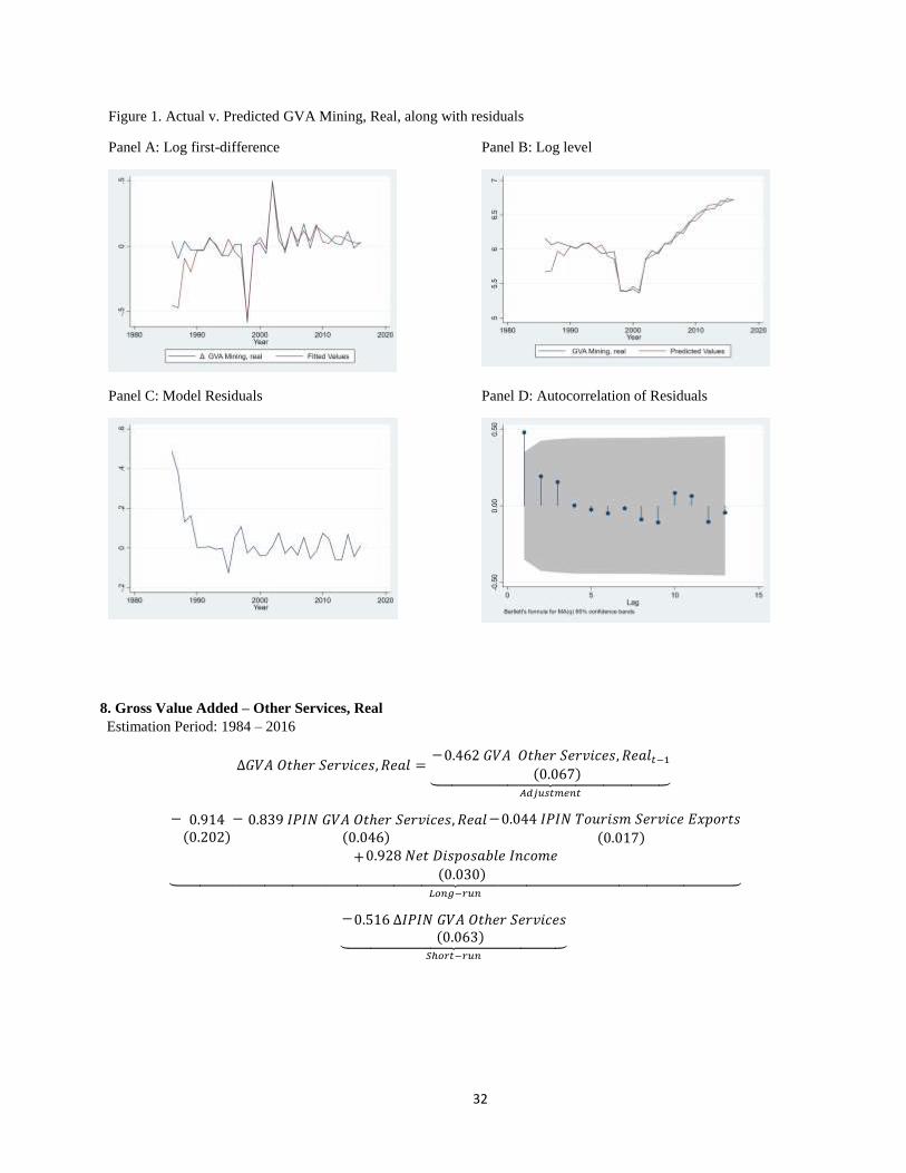
32
Figure 1. Actual v. Predicted GVA Mining, Real, along with residuals
Panel A: Log first-difference Panel B: Log level
Panel C: Model Residuals Panel D: Autocorrelation of Residuals
8. Gross Value Added – Other Services, Real
Estimation Period: 1984 – 2016
∆𝐺𝑉𝐴 𝑂𝑡ℎ𝑒𝑟 𝑆𝑒𝑟𝑣𝑖𝑐𝑒𝑠, 𝑅𝑒𝑎𝑙 =−0.462 𝐺𝑉𝐴 𝑂𝑡ℎ𝑒𝑟 𝑆𝑒𝑟𝑣𝑖𝑐𝑒𝑠, 𝑅𝑒𝑎𝑙𝑡−1
(0.067)⏟ 𝐴𝑑𝑗𝑢𝑠𝑡𝑚𝑒𝑛𝑡
− 0.914(0.202)
− 0.839 𝐼𝑃𝐼𝑁 𝐺𝑉𝐴 𝑂𝑡ℎ𝑒𝑟 𝑆𝑒𝑟𝑣𝑖𝑐𝑒𝑠, 𝑅𝑒𝑎𝑙(0.046)
−0.044 𝐼𝑃𝐼𝑁 𝑇𝑜𝑢𝑟𝑖𝑠𝑚 𝑆𝑒𝑟𝑣𝑖𝑐𝑒 𝐸𝑥𝑝𝑜𝑟𝑡𝑠(0.017)
+0.928 𝑁𝑒𝑡 𝐷𝑖𝑠𝑝𝑜𝑠𝑎𝑏𝑙𝑒 𝐼𝑛𝑐𝑜𝑚𝑒(0.030)⏟
𝐿𝑜𝑛𝑔−𝑟𝑢𝑛
−0.516 ∆𝐼𝑃𝐼𝑁 𝐺𝑉𝐴 𝑂𝑡ℎ𝑒𝑟 𝑆𝑒𝑟𝑣𝑖𝑐𝑒𝑠(0.063)⏟
𝑆ℎ𝑜𝑟𝑡−𝑟𝑢𝑛
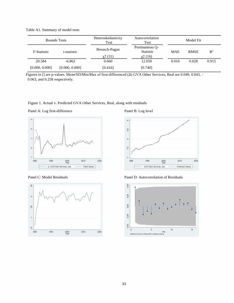
33
Table A1. Summary of model tests
Bounds Tests Heteroskedasticity
Test Autocorrelation
Test Model Fit
F-Statistic t-statistic Breusch-Pagan Portmanteau Q-
Statistic MAE RMSE R2
χ2 (31) χ2 (16)
20.584 -6.862 0.660 12.050 0.016 0.028 0.915
[0.000, 0.000] [0.000, 0.000] [0.416] [0.740]
Figures in [] are p-values. Mean/SD/Min/Max of first-differenced (∆) GVA Other Services, Real are 0.049, 0.043, -
0.063, and 0.258 respectively.
Figure 1. Actual v. Predicted GVA Other Services, Real, along with residuals
Panel A: Log first-difference Panel B: Log level
Panel C: Model Residuals Panel D: Autocorrelation of Residuals
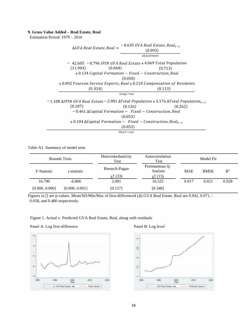
34
9. Gross Value Added – Real Estate, Real
Estimation Period: 1979 – 2016
∆𝐺𝑉𝐴 𝑅𝑒𝑎𝑙 𝐸𝑠𝑡𝑎𝑡𝑒, 𝑅𝑒𝑎𝑙 =−0.635 𝐺𝑉𝐴 𝑅𝑒𝑎𝑙 𝐸𝑠𝑡𝑎𝑡𝑒, 𝑅𝑒𝑎𝑙𝑡−1
(0.093)⏟ 𝐴𝑑𝑗𝑢𝑠𝑡𝑚𝑒𝑛𝑡
− 42.605(11.904)
−0.796 𝐼𝑃𝐼𝑁 𝐺𝑉𝐴 𝑅𝑒𝑎𝑙 𝐸𝑠𝑡𝑎𝑡𝑒(0.068)
+4.069 𝑇𝑜𝑡𝑎𝑙 𝑃𝑜𝑝𝑢𝑙𝑎𝑡𝑖𝑜𝑛
(0.713)
+0.134 𝐶𝑎𝑝𝑖𝑡𝑎𝑙 𝐹𝑜𝑟𝑚𝑎𝑡𝑖𝑜𝑛 − 𝐹𝑖𝑥𝑒𝑑 − 𝐶𝑜𝑛𝑠𝑡𝑟𝑢𝑐𝑡𝑖𝑜𝑛, 𝑅𝑒𝑎𝑙
(0.058)
+0.092 𝑇𝑜𝑢𝑟𝑖𝑠𝑚 𝑆𝑒𝑟𝑣𝑖𝑐𝑒 𝐸𝑥𝑝𝑜𝑟𝑡𝑠, 𝑅𝑒𝑎𝑙(0. 024)
+0.210 𝐶𝑜𝑚𝑝𝑒𝑛𝑠𝑎𝑡𝑖𝑜𝑛 𝑜𝑓 𝑅𝑒𝑠𝑖𝑑𝑒𝑛𝑡𝑠
(0.113)⏟ 𝐿𝑜𝑛𝑔−𝑟𝑢𝑛
−1.108 ∆𝐼𝑃𝐼𝑁 𝐺𝑉𝐴 𝑅𝑒𝑎𝑙 𝐸𝑠𝑡𝑎𝑡𝑒(0.187)
−2.981 ∆𝑇𝑜𝑡𝑎𝑙 𝑃𝑜𝑝𝑢𝑙𝑎𝑡𝑖𝑜𝑛(0.126)
+3.176 ∆𝑇𝑜𝑡𝑎𝑙 𝑃𝑜𝑝𝑢𝑙𝑎𝑡𝑖𝑜𝑛𝑡−1(0.262)
−0.461 ∆𝐶𝑎𝑝𝑖𝑡𝑎𝑙 𝐹𝑜𝑟𝑚𝑎𝑡𝑖𝑜𝑛 − 𝐹𝑖𝑥𝑒𝑑 − 𝐶𝑜𝑛𝑠𝑡𝑟𝑢𝑐𝑡𝑖𝑜𝑛, 𝑅𝑒𝑎𝑙(0.053)
+0.104 ∆𝐶𝑎𝑝𝑖𝑡𝑎𝑙 𝐹𝑜𝑟𝑚𝑎𝑡𝑖𝑜𝑛 − 𝐹𝑖𝑥𝑒𝑑 − 𝐶𝑜𝑛𝑠𝑡𝑟𝑢𝑐𝑡𝑖𝑜𝑛, 𝑅𝑒𝑎𝑙𝑡−1(0.053)⏟
𝑆ℎ𝑜𝑟𝑡−𝑟𝑢𝑛
Table A1. Summary of model tests
Bounds Tests Heteroskedasticity
Test Autocorrelation
Test Model Fit
F-Statistic t-statistic Breusch-Pagan Portmanteau Q-
Statistic MAE RMSE R2
χ2 (33) χ2 (15)
16.790 -6.806 2.001 16.525 0.017 0.021 0.928
[0.000, 0.000] [0.000, 0.001] [0.157] [0.348]
Figures in [] are p-values. Mean/SD/Min/Max of first-differenced (∆) GVA Real Estate, Real are 0.042, 0.071, -
0.058, and 0.480 respectively.
Figure 1. Actual v. Predicted GVA Real Estate, Real, along with residuals
Panel A: Log first-difference Panel B: Log level

35
Panel C: Model Residuals Panel D: Autocorrelation of Residuals
10. Gross Value Added – Trade, Real
Estimation Period: 1981 – 2016
∆𝐺𝑉𝐴 𝑇𝑟𝑎𝑑𝑒, 𝑅𝑒𝑎𝑙 =−0.539 𝐺𝑉𝐴 𝑇𝑟𝑎𝑑𝑒, 𝑅𝑒𝑎𝑙𝑡−1
(0.143)⏟ 𝐴𝑑𝑗𝑢𝑠𝑡𝑚𝑒𝑛𝑡
− 4.501(1.225)
−0.339 𝐼𝑃𝐼𝑁 𝐺𝑉𝐴 𝑇𝑟𝑎𝑑𝑒(0.062)
+1.181 𝐻𝑜𝑢𝑠𝑒ℎ𝑜𝑙𝑑 𝐶𝑜𝑛𝑠𝑢𝑚𝑝𝑡𝑖𝑜𝑛 − 𝑇𝑜𝑡𝑎𝑙
(0.055)
+0.257 𝐼𝑃𝐼𝑁 𝐺𝑉𝐴 𝐴𝑔𝑟𝑖𝑐𝑢𝑙𝑡𝑢𝑟𝑒
(0. 070)⏟ 𝐿𝑜𝑛𝑔−𝑟𝑢𝑛
−0.360 ∆𝐼𝑃𝐼𝑁 𝐺𝑉𝐴 𝑇𝑟𝑎𝑑𝑒(0.076)
+0.168 ∆𝐼𝑃𝐼𝑁 𝐺𝑉𝐴 𝐴𝑔𝑟𝑖𝑐𝑢𝑙𝑡𝑢𝑟𝑒
(0.072)⏟ 𝑆ℎ𝑜𝑟𝑡−𝑟𝑢𝑛
Table A1. Summary of model tests
Bounds Tests Heteroskedasticity
Test Autocorrelation
Test Model Fit
F-Statistic t-statistic Breusch-Pagan Portmanteau Q-
Statistic MAE RMSE R2
χ2 (34) χ2 (18)
4.398 -3.770 1.098 16.256 0.019 0.025 0.820
[0.021, 0.078] [0.007, 0.058] [0.294] [0.574]
Figures in [] are p-values. Mean/SD/Min/Max of first-differenced (∆) GVA Trade, Real are 0.042, 0.042, -0.177, and
0.083 respectively.
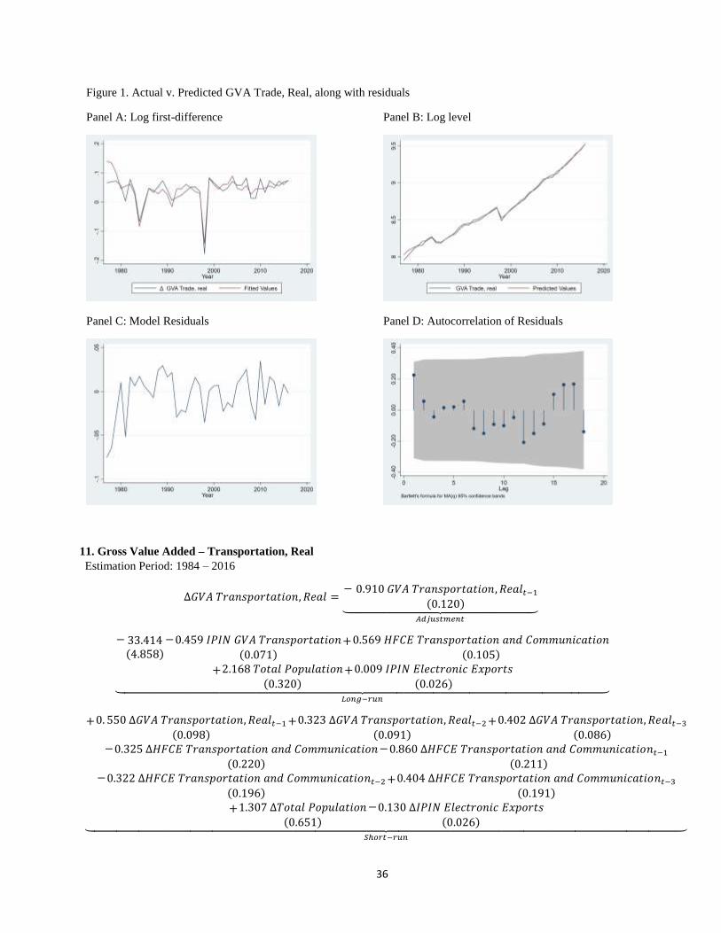
36
Figure 1. Actual v. Predicted GVA Trade, Real, along with residuals
Panel A: Log first-difference Panel B: Log level
Panel C: Model Residuals Panel D: Autocorrelation of Residuals
11. Gross Value Added – Transportation, Real
Estimation Period: 1984 – 2016
∆𝐺𝑉𝐴 𝑇𝑟𝑎𝑛𝑠𝑝𝑜𝑟𝑡𝑎𝑡𝑖𝑜𝑛, 𝑅𝑒𝑎𝑙 =− 0.910 𝐺𝑉𝐴 𝑇𝑟𝑎𝑛𝑠𝑝𝑜𝑟𝑡𝑎𝑡𝑖𝑜𝑛, 𝑅𝑒𝑎𝑙𝑡−1
(0.120)⏟ 𝐴𝑑𝑗𝑢𝑠𝑡𝑚𝑒𝑛𝑡
− 33.414(4.858)
−0.459 𝐼𝑃𝐼𝑁 𝐺𝑉𝐴 𝑇𝑟𝑎𝑛𝑠𝑝𝑜𝑟𝑡𝑎𝑡𝑖𝑜𝑛(0.071)
+0.569 𝐻𝐹𝐶𝐸 𝑇𝑟𝑎𝑛𝑠𝑝𝑜𝑟𝑡𝑎𝑡𝑖𝑜𝑛 𝑎𝑛𝑑 𝐶𝑜𝑚𝑚𝑢𝑛𝑖𝑐𝑎𝑡𝑖𝑜𝑛(0.105)
+2.168 𝑇𝑜𝑡𝑎𝑙 𝑃𝑜𝑝𝑢𝑙𝑎𝑡𝑖𝑜𝑛(0.320)
+0.009 𝐼𝑃𝐼𝑁 𝐸𝑙𝑒𝑐𝑡𝑟𝑜𝑛𝑖𝑐 𝐸𝑥𝑝𝑜𝑟𝑡𝑠(0.026)⏟
𝐿𝑜𝑛𝑔−𝑟𝑢𝑛
+0. 550 ∆𝐺𝑉𝐴 𝑇𝑟𝑎𝑛𝑠𝑝𝑜𝑟𝑡𝑎𝑡𝑖𝑜𝑛, 𝑅𝑒𝑎𝑙𝑡−1(0.098)
+0.323 ∆𝐺𝑉𝐴 𝑇𝑟𝑎𝑛𝑠𝑝𝑜𝑟𝑡𝑎𝑡𝑖𝑜𝑛, 𝑅𝑒𝑎𝑙𝑡−2(0.091)
+0.402 ∆𝐺𝑉𝐴 𝑇𝑟𝑎𝑛𝑠𝑝𝑜𝑟𝑡𝑎𝑡𝑖𝑜𝑛, 𝑅𝑒𝑎𝑙𝑡−3(0.086)
−0.325 ∆𝐻𝐹𝐶𝐸 𝑇𝑟𝑎𝑛𝑠𝑝𝑜𝑟𝑡𝑎𝑡𝑖𝑜𝑛 𝑎𝑛𝑑 𝐶𝑜𝑚𝑚𝑢𝑛𝑖𝑐𝑎𝑡𝑖𝑜𝑛(0.220)
−0.860 ∆𝐻𝐹𝐶𝐸 𝑇𝑟𝑎𝑛𝑠𝑝𝑜𝑟𝑡𝑎𝑡𝑖𝑜𝑛 𝑎𝑛𝑑 𝐶𝑜𝑚𝑚𝑢𝑛𝑖𝑐𝑎𝑡𝑖𝑜𝑛𝑡−1(0.211)
−0.322 ∆𝐻𝐹𝐶𝐸 𝑇𝑟𝑎𝑛𝑠𝑝𝑜𝑟𝑡𝑎𝑡𝑖𝑜𝑛 𝑎𝑛𝑑 𝐶𝑜𝑚𝑚𝑢𝑛𝑖𝑐𝑎𝑡𝑖𝑜𝑛𝑡−2(0.196)
+0.404 ∆𝐻𝐹𝐶𝐸 𝑇𝑟𝑎𝑛𝑠𝑝𝑜𝑟𝑡𝑎𝑡𝑖𝑜𝑛 𝑎𝑛𝑑 𝐶𝑜𝑚𝑚𝑢𝑛𝑖𝑐𝑎𝑡𝑖𝑜𝑛𝑡−3(0.191)
+1.307 ∆𝑇𝑜𝑡𝑎𝑙 𝑃𝑜𝑝𝑢𝑙𝑎𝑡𝑖𝑜𝑛(0.651)
−0.130 ∆𝐼𝑃𝐼𝑁 𝐸𝑙𝑒𝑐𝑡𝑟𝑜𝑛𝑖𝑐 𝐸𝑥𝑝𝑜𝑟𝑡𝑠(0.026)⏟
𝑆ℎ𝑜𝑟𝑡−𝑟𝑢𝑛
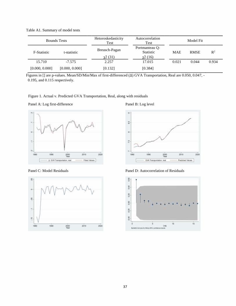
37
Table A1. Summary of model tests
Bounds Tests Hetoroskedasticity
Test Autocorrelation
Test Model Fit
F-Statistic t-statistic Breusch-Pagan Portmanteau Q-
Statistic MAE RMSE R2
χ2 (31) χ2 (16)
15.710 -7.575 2.257 17.015 0.021 0.044 0.934
[0.000, 0.000] [0.000, 0.000] [0.132] [0.384]
Figures in [] are p-values. Mean/SD/Min/Max of first-differenced (∆) GVA Transportation, Real are 0.050, 0.047, -
0.195, and 0.115 respectively.
Figure 1. Actual v. Predicted GVA Transportation, Real, along with residuals
Panel A: Log first-difference Panel B: Log level
Panel C: Model Residuals Panel D: Autocorrelation of Residuals

38
12. Gross Value Added – Water, Real
Estimation Period: 1983 – 2016
∆𝐺𝑉𝐴 𝑊𝑎𝑡𝑒𝑟, 𝑅𝑒𝑎𝑙 =−0.976 𝐺𝑉𝐴 𝑊𝑎𝑡𝑒𝑟, 𝑅𝑒𝑎𝑙𝑡−1
(0.126)⏟ 𝐴𝑑𝑗𝑢𝑠𝑡𝑚𝑒𝑛𝑡
− 57.793(7.499)
−0.546 𝐼𝑃𝐼𝑁 𝐺𝑉𝐴 𝑊𝑎𝑡𝑒𝑟(0.052)
+3.482 𝑇𝑜𝑡𝑎𝑙 𝑃𝑜𝑝𝑢𝑙𝑎𝑡𝑖𝑜𝑛(0.230)
+0.706 𝐺𝑉𝐴 𝑆𝑒𝑟𝑣𝑖𝑐𝑒, 𝑅𝑒𝑎𝑙(0.094)
−0.448 𝐶𝑎𝑝𝑖𝑡𝑎𝑙 𝐹𝑜𝑟𝑚𝑎𝑡𝑖𝑜𝑛 − 𝐹𝑖𝑥𝑒𝑑 − 𝐶𝑜𝑛𝑠𝑡𝑟𝑢𝑐𝑡𝑖𝑜𝑛, 𝑅𝑒𝑎𝑙(0.050)⏟
𝐿𝑜𝑛𝑔−𝑟𝑢𝑛
−0.018 ∆𝐼𝑃𝐼𝑁 𝐺𝑉𝐴 𝑊𝑎𝑡𝑒𝑟(0.080)
+0.065 ∆𝐼𝑃𝐼𝑁 𝐺𝑉𝐴 𝑊𝑎𝑡𝑒𝑟𝑡−1(0.046)
−0.172 ∆𝐼𝑃𝐼𝑁 𝐺𝑉𝐴 𝑊𝑎𝑡𝑒𝑟𝑡−2(0.049)
−4.521 ∆𝑇𝑜𝑡𝑎𝑙 𝑃𝑜𝑝𝑢𝑙𝑎𝑡𝑖𝑜𝑛(0.159)
−0.003 ∆𝐶𝑎𝑝𝑖𝑡𝑎𝑙 𝐹𝑜𝑟𝑚𝑎𝑡𝑖𝑜𝑛 − 𝐹𝑖𝑥𝑒𝑑 − 𝐶𝑜𝑛𝑠𝑡𝑟𝑢𝑐𝑡𝑖𝑜𝑛, 𝑅𝑒𝑎𝑙(0.046)
+0.126 ∆𝐶𝑎𝑝𝑖𝑡𝑎𝑙 𝐹𝑜𝑟𝑚𝑎𝑡𝑖𝑜𝑛 − 𝐹𝑖𝑥𝑒𝑑 − 𝐶𝑜𝑛𝑠𝑡𝑟𝑢𝑐𝑡𝑖𝑜𝑛, 𝑅𝑒𝑎𝑙𝑡−1(0.051)⏟
𝑆ℎ𝑜𝑟𝑡−𝑟𝑢𝑛
Table A1. Summary of model tests
Bounds Tests Hetoroskedasticity
Test Autocorrelation
Test Model Fit
F-Statistic t-statistic Breusch-Pagan Portmanteau Q-
Statistic MAE RMSE R2
χ2 (32) χ2 (16)
22.856 -7.697 0.005 8.404 0.029 0.067 0.932
[0.000, 0.000] [0.000, 0.000] [0.942] [0.935]
Figures in [] are p-values. Mean/SD/Min/Max of first-differenced (∆) GVA Water, Real are 0.072, 0.090, -0.075, and
0.361 respectively.
Figure 1. Actual v. Predicted GVA Water, Real, along with residuals
Panel A: Log first-difference Panel B: Log level
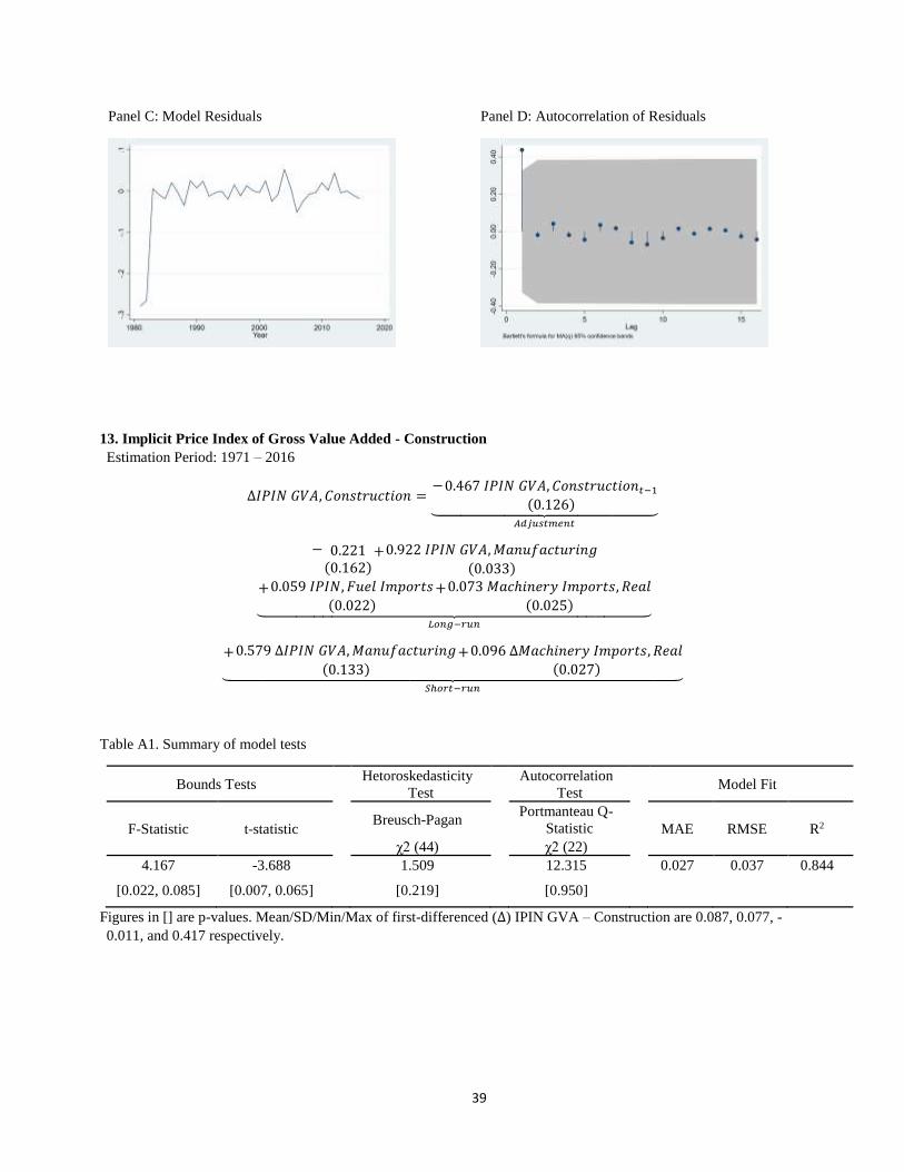
39
Panel C: Model Residuals Panel D: Autocorrelation of Residuals
13. Implicit Price Index of Gross Value Added - Construction
Estimation Period: 1971 – 2016
∆𝐼𝑃𝐼𝑁 𝐺𝑉𝐴, 𝐶𝑜𝑛𝑠𝑡𝑟𝑢𝑐𝑡𝑖𝑜𝑛 =−0.467 𝐼𝑃𝐼𝑁 𝐺𝑉𝐴, 𝐶𝑜𝑛𝑠𝑡𝑟𝑢𝑐𝑡𝑖𝑜𝑛𝑡−1
(0.126)⏟ 𝐴𝑑𝑗𝑢𝑠𝑡𝑚𝑒𝑛𝑡
− 0.221(0.162)
+0.922 𝐼𝑃𝐼𝑁 𝐺𝑉𝐴,𝑀𝑎𝑛𝑢𝑓𝑎𝑐𝑡𝑢𝑟𝑖𝑛𝑔
(0.033)
+0.059 𝐼𝑃𝐼𝑁, 𝐹𝑢𝑒𝑙 𝐼𝑚𝑝𝑜𝑟𝑡𝑠
(0.022)+0.073 𝑀𝑎𝑐ℎ𝑖𝑛𝑒𝑟𝑦 𝐼𝑚𝑝𝑜𝑟𝑡𝑠, 𝑅𝑒𝑎𝑙
(0.025)⏟ 𝐿𝑜𝑛𝑔−𝑟𝑢𝑛
+0.579 ∆𝐼𝑃𝐼𝑁 𝐺𝑉𝐴,𝑀𝑎𝑛𝑢𝑓𝑎𝑐𝑡𝑢𝑟𝑖𝑛𝑔
(0.133)+0.096 ∆𝑀𝑎𝑐ℎ𝑖𝑛𝑒𝑟𝑦 𝐼𝑚𝑝𝑜𝑟𝑡𝑠, 𝑅𝑒𝑎𝑙
(0.027)⏟ 𝑆ℎ𝑜𝑟𝑡−𝑟𝑢𝑛
Table A1. Summary of model tests
Bounds Tests Hetoroskedasticity
Test Autocorrelation
Test Model Fit
F-Statistic t-statistic Breusch-Pagan Portmanteau Q-
Statistic MAE RMSE R2
χ2 (44) χ2 (22)
4.167 -3.688 1.509 12.315 0.027 0.037 0.844
[0.022, 0.085] [0.007, 0.065] [0.219] [0.950]
Figures in [] are p-values. Mean/SD/Min/Max of first-differenced (∆) IPIN GVA – Construction are 0.087, 0.077, -
0.011, and 0.417 respectively.

40
Figure 1. Actual v. Predicted IPIN GVA – Construction, along with residuals
Panel A: Log first-difference Panel B: Log level
Panel C: Model Residuals Panel D: Autocorrelation of Residuals
14. Implicit Price Index of Gross Value Added – Electricity and Steam
Estimation Period: 1984 – 2016
∆𝐼𝑃𝐼𝑁 𝐺𝑉𝐴, 𝐸𝑙𝑒𝑐𝑡𝑟𝑖𝑐𝑖𝑡𝑦 𝑎𝑛𝑑 𝑆𝑡𝑒𝑎𝑚 =− 0.725 𝐼𝑃𝐼𝑁 𝐺𝑉𝐴, 𝐸𝑙𝑒𝑐𝑡𝑟𝑖𝑐𝑖𝑡𝑦 𝑎𝑛𝑑 𝑆𝑡𝑒𝑎𝑚𝑡−1
(0.133)⏟ 𝐴𝑑𝑗𝑢𝑠𝑡𝑚𝑒𝑛𝑡
− 21.418(4.688)
+0.844 𝑊𝑎𝑔𝑒 𝐼𝑛𝑑𝑒𝑥, 𝐸𝑙𝑒𝑐𝑡𝑟𝑖𝑐𝑖𝑡𝑦 𝑎𝑛𝑑 𝑆𝑡𝑒𝑎𝑚
(0.238)
+0.710 𝐼𝑃𝐼𝑁 𝐶𝑎𝑝𝑖𝑡𝑎𝑙 𝐹𝑜𝑟𝑚𝑎𝑡𝑖𝑜𝑛 − 𝐹𝑖𝑥𝑒𝑑 − 𝐷𝑢𝑟𝑎𝑏𝑙𝑒𝑠(0.077)
+1.451 𝑇𝑜𝑡𝑎𝑙 𝑃𝑜𝑝𝑢𝑙𝑎𝑡𝑖𝑜𝑛
(0.195)⏟ 𝐿𝑜𝑛𝑔−𝑟𝑢𝑛
−0.457 ∆𝑊𝑎𝑔𝑒 𝐼𝑛𝑑𝑒𝑥, 𝐸𝑙𝑒𝑐𝑡𝑟𝑖𝑐𝑖𝑡𝑦 𝑎𝑛𝑑 𝑆𝑡𝑒𝑎𝑚
(0.136)
−0.325 ∆𝑊𝑎𝑔𝑒 𝐼𝑛𝑑𝑒𝑥, 𝐸𝑙𝑒𝑐𝑡𝑟𝑖𝑐𝑖𝑡𝑦 𝑎𝑛𝑑 𝑆𝑡𝑒𝑎𝑚𝑡−1
(0.112)
+0.382 ∆𝐼𝑃𝐼𝑁 𝐶𝑎𝑝𝑖𝑡𝑎𝑙 𝐹𝑜𝑟𝑚𝑎𝑡𝑖𝑜𝑛 − 𝐹𝑖𝑥𝑒𝑑 − 𝐷𝑢𝑟𝑎𝑏𝑙𝑒𝑠
(0.137)+0.382 ∆𝐼𝑃𝐼𝑁 𝐶𝑎𝑝𝑖𝑡𝑎𝑙 𝐹𝑜𝑟𝑚𝑎𝑡𝑖𝑜𝑛 − 𝐹𝑖𝑥𝑒𝑑 − 𝐷𝑢𝑟𝑎𝑏𝑙𝑒𝑠𝑡−1
(0.132)⏟ 𝑆ℎ𝑜𝑟𝑡−𝑟𝑢𝑛
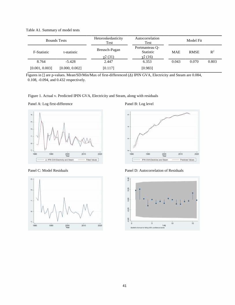
41
Table A1. Summary of model tests
Bounds Tests Hetoroskedasticity
Test Autocorrelation
Test Model Fit
F-Statistic t-statistic Breusch-Pagan Portmanteau Q-
Statistic MAE RMSE R2
χ2 (31) χ2 (16)
8.764 -5.428 2.447 6.353 0.043 0.070 0.803
[0.001, 0.003] [0.000, 0.002] [0.117] [0.983]
Figures in [] are p-values. Mean/SD/Min/Max of first-differenced (∆) IPIN GVA, Electricity and Steam are 0.084,
0.108, -0.094, and 0.432 respectively.
Figure 1. Actual v. Predicted IPIN GVA, Electricity and Steam, along with residuals
Panel A: Log first-difference Panel B: Log level
Panel C: Model Residuals Panel D: Autocorrelation of Residuals
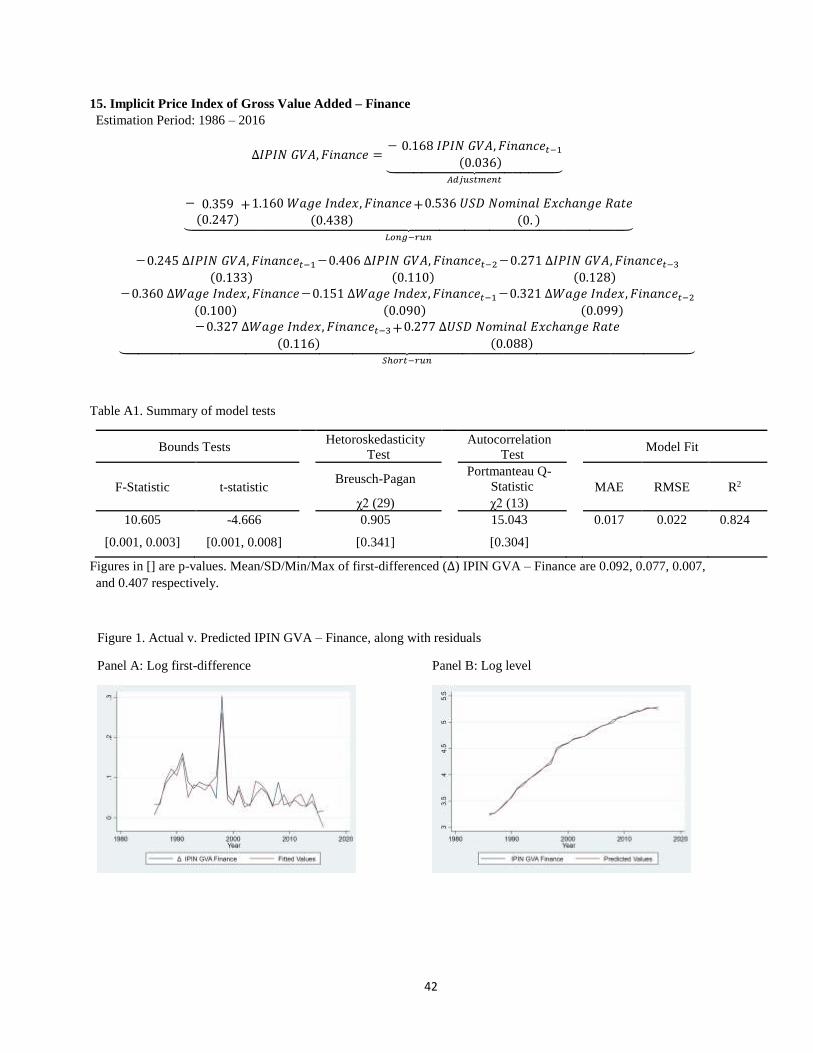
42
15. Implicit Price Index of Gross Value Added – Finance
Estimation Period: 1986 – 2016
∆𝐼𝑃𝐼𝑁 𝐺𝑉𝐴, 𝐹𝑖𝑛𝑎𝑛𝑐𝑒 =− 0.168 𝐼𝑃𝐼𝑁 𝐺𝑉𝐴, 𝐹𝑖𝑛𝑎𝑛𝑐𝑒𝑡−1
(0.036)⏟ 𝐴𝑑𝑗𝑢𝑠𝑡𝑚𝑒𝑛𝑡
− 0.359(0.247)
+1.160 𝑊𝑎𝑔𝑒 𝐼𝑛𝑑𝑒𝑥, 𝐹𝑖𝑛𝑎𝑛𝑐𝑒
(0.438)+0.536 𝑈𝑆𝐷 𝑁𝑜𝑚𝑖𝑛𝑎𝑙 𝐸𝑥𝑐ℎ𝑎𝑛𝑔𝑒 𝑅𝑎𝑡𝑒
(0. )⏟ 𝐿𝑜𝑛𝑔−𝑟𝑢𝑛
−0.245 ∆𝐼𝑃𝐼𝑁 𝐺𝑉𝐴, 𝐹𝑖𝑛𝑎𝑛𝑐𝑒𝑡−1(0.133)
−0.406 ∆𝐼𝑃𝐼𝑁 𝐺𝑉𝐴, 𝐹𝑖𝑛𝑎𝑛𝑐𝑒𝑡−2(0.110)
−0.271 ∆𝐼𝑃𝐼𝑁 𝐺𝑉𝐴, 𝐹𝑖𝑛𝑎𝑛𝑐𝑒𝑡−3(0.128)
−0.360 ∆𝑊𝑎𝑔𝑒 𝐼𝑛𝑑𝑒𝑥, 𝐹𝑖𝑛𝑎𝑛𝑐𝑒
(0.100)
−0.151 ∆𝑊𝑎𝑔𝑒 𝐼𝑛𝑑𝑒𝑥, 𝐹𝑖𝑛𝑎𝑛𝑐𝑒𝑡−1(0.090)
−0.321 ∆𝑊𝑎𝑔𝑒 𝐼𝑛𝑑𝑒𝑥, 𝐹𝑖𝑛𝑎𝑛𝑐𝑒𝑡−2(0.099)
−0.327 ∆𝑊𝑎𝑔𝑒 𝐼𝑛𝑑𝑒𝑥, 𝐹𝑖𝑛𝑎𝑛𝑐𝑒𝑡−3(0.116)
+0.277 ∆𝑈𝑆𝐷 𝑁𝑜𝑚𝑖𝑛𝑎𝑙 𝐸𝑥𝑐ℎ𝑎𝑛𝑔𝑒 𝑅𝑎𝑡𝑒
(0.088)⏟ 𝑆ℎ𝑜𝑟𝑡−𝑟𝑢𝑛
Table A1. Summary of model tests
Bounds Tests Hetoroskedasticity
Test Autocorrelation
Test Model Fit
F-Statistic t-statistic Breusch-Pagan Portmanteau Q-
Statistic MAE RMSE R2
χ2 (29) χ2 (13)
10.605 -4.666 0.905 15.043 0.017 0.022 0.824
[0.001, 0.003] [0.001, 0.008] [0.341] [0.304]
Figures in [] are p-values. Mean/SD/Min/Max of first-differenced (∆) IPIN GVA – Finance are 0.092, 0.077, 0.007,
and 0.407 respectively.
Figure 1. Actual v. Predicted IPIN GVA – Finance, along with residuals
Panel A: Log first-difference Panel B: Log level
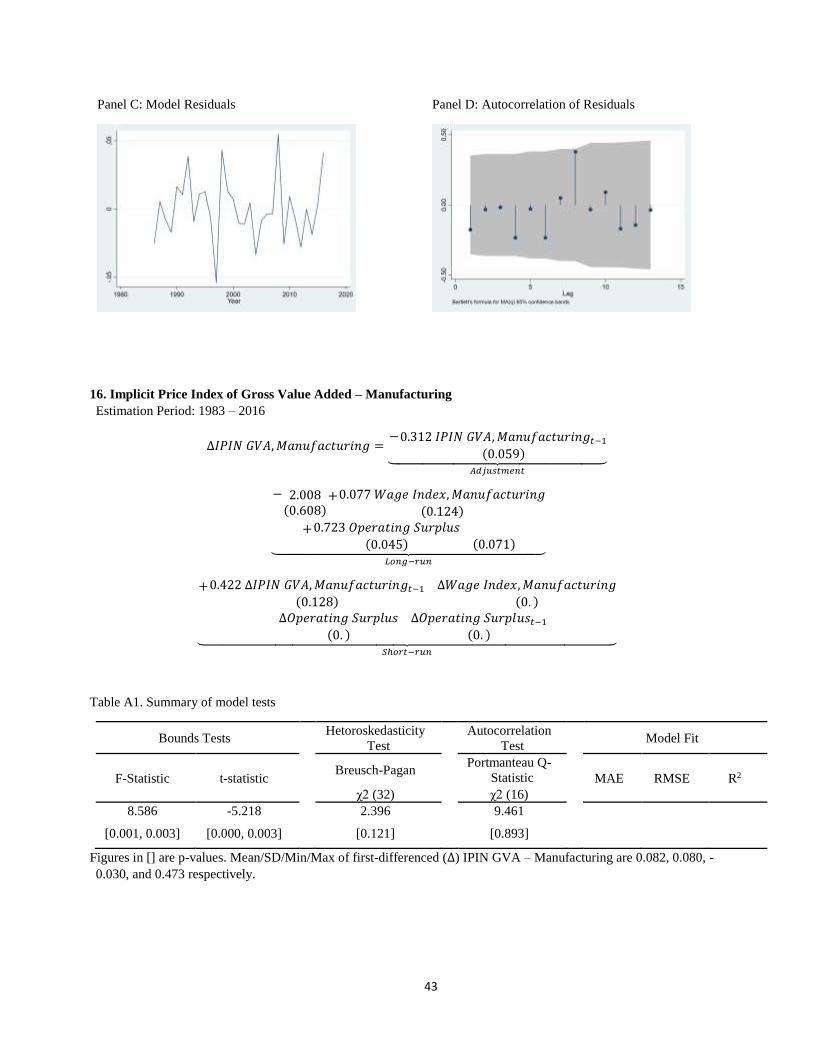
43
Panel C: Model Residuals Panel D: Autocorrelation of Residuals
16. Implicit Price Index of Gross Value Added – Manufacturing
Estimation Period: 1983 – 2016
∆𝐼𝑃𝐼𝑁 𝐺𝑉𝐴,𝑀𝑎𝑛𝑢𝑓𝑎𝑐𝑡𝑢𝑟𝑖𝑛𝑔 =−0.312 𝐼𝑃𝐼𝑁 𝐺𝑉𝐴,𝑀𝑎𝑛𝑢𝑓𝑎𝑐𝑡𝑢𝑟𝑖𝑛𝑔𝑡−1
(0.059)⏟ 𝐴𝑑𝑗𝑢𝑠𝑡𝑚𝑒𝑛𝑡
− 2.008(0.608)
+0.077 𝑊𝑎𝑔𝑒 𝐼𝑛𝑑𝑒𝑥,𝑀𝑎𝑛𝑢𝑓𝑎𝑐𝑡𝑢𝑟𝑖𝑛𝑔
(0.124)
+0.723 𝑂𝑝𝑒𝑟𝑎𝑡𝑖𝑛𝑔 𝑆𝑢𝑟𝑝𝑙𝑢𝑠
(0.045) (0.071)⏟ 𝐿𝑜𝑛𝑔−𝑟𝑢𝑛
+0.422 ∆𝐼𝑃𝐼𝑁 𝐺𝑉𝐴,𝑀𝑎𝑛𝑢𝑓𝑎𝑐𝑡𝑢𝑟𝑖𝑛𝑔𝑡−1(0.128)
∆𝑊𝑎𝑔𝑒 𝐼𝑛𝑑𝑒𝑥,𝑀𝑎𝑛𝑢𝑓𝑎𝑐𝑡𝑢𝑟𝑖𝑛𝑔
(0. )∆𝑂𝑝𝑒𝑟𝑎𝑡𝑖𝑛𝑔 𝑆𝑢𝑟𝑝𝑙𝑢𝑠
(0. )
∆𝑂𝑝𝑒𝑟𝑎𝑡𝑖𝑛𝑔 𝑆𝑢𝑟𝑝𝑙𝑢𝑠𝑡−1(0. )⏟
𝑆ℎ𝑜𝑟𝑡−𝑟𝑢𝑛
Table A1. Summary of model tests
Bounds Tests Hetoroskedasticity
Test Autocorrelation
Test Model Fit
F-Statistic t-statistic Breusch-Pagan Portmanteau Q-
Statistic MAE RMSE R2
χ2 (32) χ2 (16)
8.586 -5.218 2.396 9.461
[0.001, 0.003] [0.000, 0.003] [0.121] [0.893]
Figures in [] are p-values. Mean/SD/Min/Max of first-differenced (∆) IPIN GVA – Manufacturing are 0.082, 0.080, -
0.030, and 0.473 respectively.
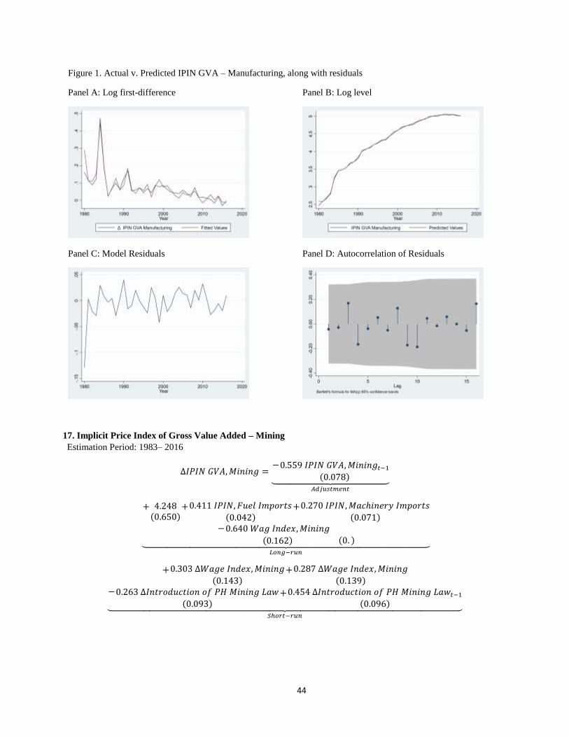
44
Figure 1. Actual v. Predicted IPIN GVA – Manufacturing, along with residuals
Panel A: Log first-difference Panel B: Log level
Panel C: Model Residuals Panel D: Autocorrelation of Residuals
17. Implicit Price Index of Gross Value Added – Mining
Estimation Period: 1983– 2016
∆𝐼𝑃𝐼𝑁 𝐺𝑉𝐴,𝑀𝑖𝑛𝑖𝑛𝑔 =−0.559 𝐼𝑃𝐼𝑁 𝐺𝑉𝐴,𝑀𝑖𝑛𝑖𝑛𝑔𝑡−1
(0.078)⏟ 𝐴𝑑𝑗𝑢𝑠𝑡𝑚𝑒𝑛𝑡
+ 4.248(0.650)
+0.411 𝐼𝑃𝐼𝑁, 𝐹𝑢𝑒𝑙 𝐼𝑚𝑝𝑜𝑟𝑡𝑠
(0.042)+0.270 𝐼𝑃𝐼𝑁,𝑀𝑎𝑐ℎ𝑖𝑛𝑒𝑟𝑦 𝐼𝑚𝑝𝑜𝑟𝑡𝑠
(0.071)−0.640 𝑊𝑎𝑔 𝐼𝑛𝑑𝑒𝑥,𝑀𝑖𝑛𝑖𝑛𝑔
(0.162) (0. )⏟ 𝐿𝑜𝑛𝑔−𝑟𝑢𝑛
+0.303 ∆𝑊𝑎𝑔𝑒 𝐼𝑛𝑑𝑒𝑥,𝑀𝑖𝑛𝑖𝑛𝑔
(0.143)+0.287 ∆𝑊𝑎𝑔𝑒 𝐼𝑛𝑑𝑒𝑥,𝑀𝑖𝑛𝑖𝑛𝑔
(0.139)−0.263 ∆𝐼𝑛𝑡𝑟𝑜𝑑𝑢𝑐𝑡𝑖𝑜𝑛 𝑜𝑓 𝑃𝐻 𝑀𝑖𝑛𝑖𝑛𝑔 𝐿𝑎𝑤
(0.093)+0.454 ∆𝐼𝑛𝑡𝑟𝑜𝑑𝑢𝑐𝑡𝑖𝑜𝑛 𝑜𝑓 𝑃𝐻 𝑀𝑖𝑛𝑖𝑛𝑔 𝐿𝑎𝑤𝑡−1
(0.096)⏟ 𝑆ℎ𝑜𝑟𝑡−𝑟𝑢𝑛
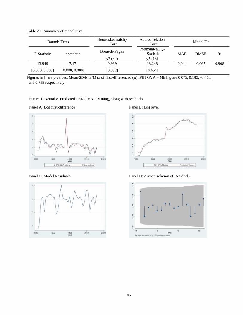
45
Table A1. Summary of model tests
Bounds Tests Hetoroskedasticity
Test Autocorrelation
Test Model Fit
F-Statistic t-statistic Breusch-Pagan Portmanteau Q-
Statistic MAE RMSE R2
χ2 (32) χ2 (16)
13.949 -7.171 0.939 13.248 0.044 0.067 0.908
[0.000, 0.000] [0.000, 0.000] [0.332] [0.654]
Figures in [] are p-values. Mean/SD/Min/Max of first-differenced (∆) IPIN GVA – Mining are 0.079, 0.185, -0.453,
and 0.755 respectively.
Figure 1. Actual v. Predicted IPIN GVA – Mining, along with residuals
Panel A: Log first-difference Panel B: Log level
Panel C: Model Residuals Panel D: Autocorrelation of Residuals
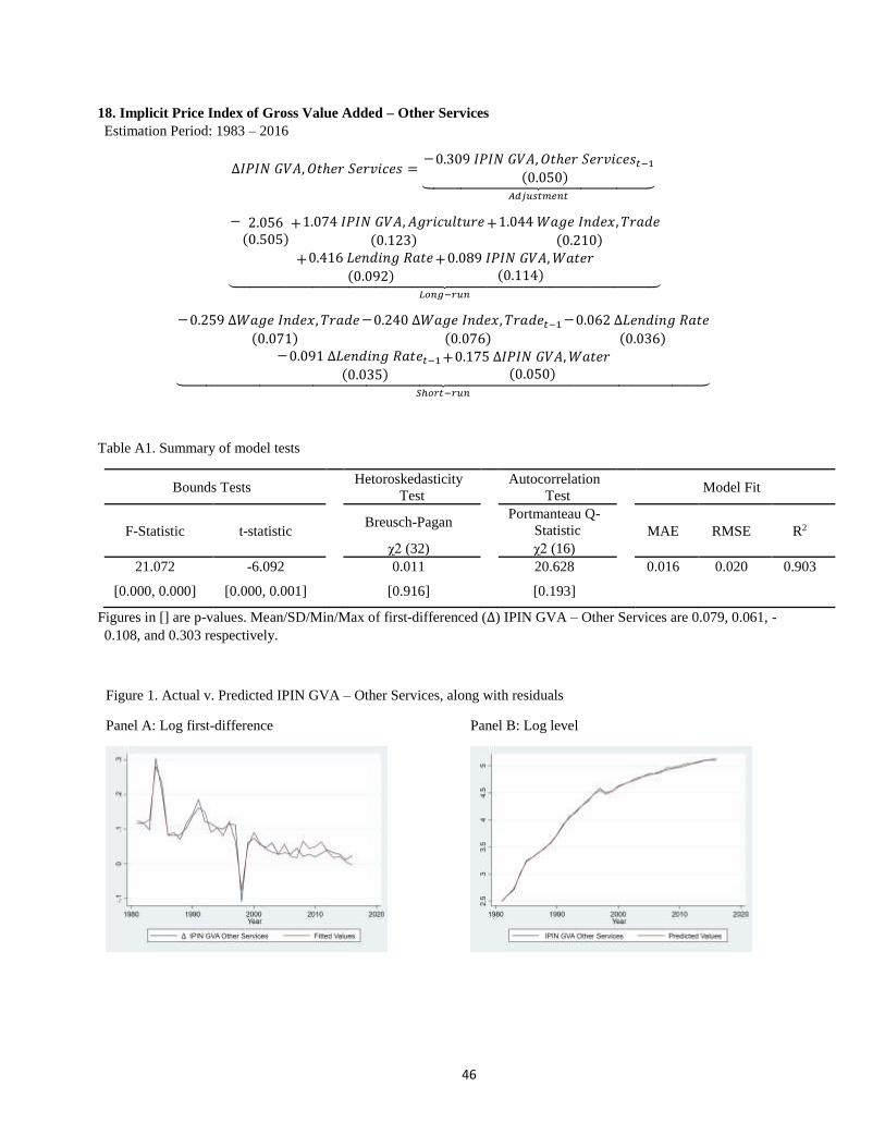
46
18. Implicit Price Index of Gross Value Added – Other Services
Estimation Period: 1983 – 2016
∆𝐼𝑃𝐼𝑁 𝐺𝑉𝐴, 𝑂𝑡ℎ𝑒𝑟 𝑆𝑒𝑟𝑣𝑖𝑐𝑒𝑠 =−0.309 𝐼𝑃𝐼𝑁 𝐺𝑉𝐴, 𝑂𝑡ℎ𝑒𝑟 𝑆𝑒𝑟𝑣𝑖𝑐𝑒𝑠𝑡−1
(0.050)⏟ 𝐴𝑑𝑗𝑢𝑠𝑡𝑚𝑒𝑛𝑡
− 2.056(0.505)
+1.074 𝐼𝑃𝐼𝑁 𝐺𝑉𝐴, 𝐴𝑔𝑟𝑖𝑐𝑢𝑙𝑡𝑢𝑟𝑒
(0.123)+1.044 𝑊𝑎𝑔𝑒 𝐼𝑛𝑑𝑒𝑥, 𝑇𝑟𝑎𝑑𝑒
(0.210)
+0.416 𝐿𝑒𝑛𝑑𝑖𝑛𝑔 𝑅𝑎𝑡𝑒
(0.092)+0.089 𝐼𝑃𝐼𝑁 𝐺𝑉𝐴,𝑊𝑎𝑡𝑒𝑟
(0.114)⏟ 𝐿𝑜𝑛𝑔−𝑟𝑢𝑛
−0.259 ∆𝑊𝑎𝑔𝑒 𝐼𝑛𝑑𝑒𝑥, 𝑇𝑟𝑎𝑑𝑒
(0.071)
−0.240 ∆𝑊𝑎𝑔𝑒 𝐼𝑛𝑑𝑒𝑥, 𝑇𝑟𝑎𝑑𝑒𝑡−1(0.076)
−0.062 ∆𝐿𝑒𝑛𝑑𝑖𝑛𝑔 𝑅𝑎𝑡𝑒
(0.036)−0.091 ∆𝐿𝑒𝑛𝑑𝑖𝑛𝑔 𝑅𝑎𝑡𝑒𝑡−1
(0.035)+0.175 ∆𝐼𝑃𝐼𝑁 𝐺𝑉𝐴,𝑊𝑎𝑡𝑒𝑟
(0.050)⏟ 𝑆ℎ𝑜𝑟𝑡−𝑟𝑢𝑛
Table A1. Summary of model tests
Bounds Tests Hetoroskedasticity
Test Autocorrelation
Test Model Fit
F-Statistic t-statistic Breusch-Pagan Portmanteau Q-
Statistic MAE RMSE R2
χ2 (32) χ2 (16)
21.072 -6.092 0.011 20.628 0.016 0.020 0.903
[0.000, 0.000] [0.000, 0.001] [0.916] [0.193]
Figures in [] are p-values. Mean/SD/Min/Max of first-differenced (∆) IPIN GVA – Other Services are 0.079, 0.061, -
0.108, and 0.303 respectively.
Figure 1. Actual v. Predicted IPIN GVA – Other Services, along with residuals
Panel A: Log first-difference Panel B: Log level
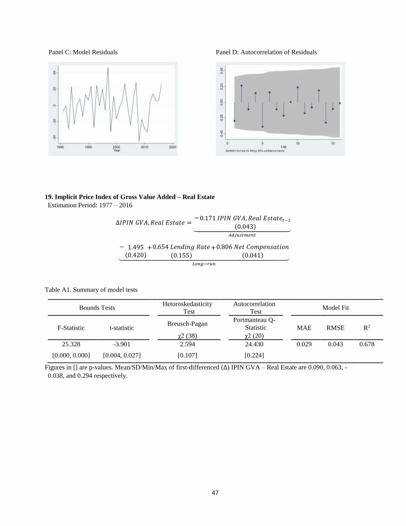
47
Panel C: Model Residuals Panel D: Autocorrelation of Residuals
19. Implicit Price Index of Gross Value Added – Real Estate
Estimation Period: 1977 – 2016
∆𝐼𝑃𝐼𝑁 𝐺𝑉𝐴, 𝑅𝑒𝑎𝑙 𝐸𝑠𝑡𝑎𝑡𝑒 =−0.171 𝐼𝑃𝐼𝑁 𝐺𝑉𝐴, 𝑅𝑒𝑎𝑙 𝐸𝑠𝑡𝑎𝑡𝑒𝑡−1
(0.043)⏟ 𝐴𝑑𝑗𝑢𝑠𝑡𝑚𝑒𝑛𝑡
− 1.495(0.420)
+0.654 𝐿𝑒𝑛𝑑𝑖𝑛𝑔 𝑅𝑎𝑡𝑒
(0.155)+0.806 𝑁𝑒𝑡 𝐶𝑜𝑚𝑝𝑒𝑛𝑠𝑎𝑡𝑖𝑜𝑛
(0.041)⏟ 𝐿𝑜𝑛𝑔−𝑟𝑢𝑛
Table A1. Summary of model tests
Bounds Tests Hetoroskedasticity
Test Autocorrelation
Test Model Fit
F-Statistic t-statistic Breusch-Pagan Portmanteau Q-
Statistic MAE RMSE R2
χ2 (38) χ2 (20)
25.328 -3.901 2.594 24.430 0.029 0.043 0.678
[0.000, 0.000] [0.004, 0.027] [0.107] [0.224]
Figures in [] are p-values. Mean/SD/Min/Max of first-differenced (∆) IPIN GVA – Real Estate are 0.090, 0.063, -
0.038, and 0.294 respectively.
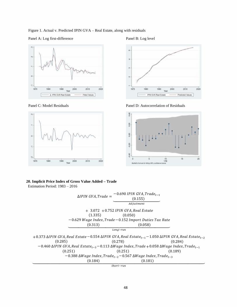
48
Figure 1. Actual v. Predicted IPIN GVA – Real Estate, along with residuals
Panel A: Log first-difference Panel B: Log level
Panel C: Model Residuals Panel D: Autocorrelation of Residuals
20. Implicit Price Index of Gross Value Added – Trade
Estimation Period: 1983 – 2016
∆𝐼𝑃𝐼𝑁 𝐺𝑉𝐴, 𝑇𝑟𝑎𝑑𝑒 =−0.690 𝐼𝑃𝐼𝑁 𝐺𝑉𝐴, 𝑇𝑟𝑎𝑑𝑒𝑡−1
(0.155)⏟ 𝐴𝑑𝑗𝑢𝑠𝑡𝑚𝑒𝑛𝑡
+ 3.072(1.335)
+0.752 𝐼𝑃𝐼𝑁 𝐺𝑉𝐴, 𝑅𝑒𝑎𝑙 𝐸𝑠𝑡𝑎𝑡𝑒(0.050)
−0.629 𝑊𝑎𝑔𝑒 𝐼𝑛𝑑𝑒𝑥, 𝑇𝑟𝑎𝑑𝑒
(0.313)
−0.152 𝐼𝑚𝑝𝑜𝑟𝑡 𝐷𝑢𝑡𝑖𝑒𝑠 𝑇𝑎𝑥 𝑅𝑎𝑡𝑒(0.058)⏟
𝐿𝑜𝑛𝑔−𝑟𝑢𝑛
+0.373 ∆𝐼𝑃𝐼𝑁 𝐺𝑉𝐴, 𝑅𝑒𝑎𝑙 𝐸𝑠𝑡𝑎𝑡𝑒(0.285)
−0.554 ∆𝐼𝑃𝐼𝑁 𝐺𝑉𝐴, 𝑅𝑒𝑎𝑙 𝐸𝑠𝑡𝑎𝑡𝑒𝑡−1(0.278)
−1.050 ∆𝐼𝑃𝐼𝑁 𝐺𝑉𝐴, 𝑅𝑒𝑎𝑙 𝐸𝑠𝑡𝑎𝑡𝑒𝑡−2(0.284)
−0.460 ∆𝐼𝑃𝐼𝑁 𝐺𝑉𝐴, 𝑅𝑒𝑎𝑙 𝐸𝑠𝑡𝑎𝑡𝑒𝑡−3(0.251)
−0.113 ∆𝑊𝑎𝑔𝑒 𝐼𝑛𝑑𝑒𝑥, 𝑇𝑟𝑎𝑑𝑒
(0.251)+0.058 ∆𝑊𝑎𝑔𝑒 𝐼𝑛𝑑𝑒𝑥, 𝑇𝑟𝑎𝑑𝑒𝑡−1
(0.189)−0.388 ∆𝑊𝑎𝑔𝑒 𝐼𝑛𝑑𝑒𝑥, 𝑇𝑟𝑎𝑑𝑒𝑡−2
(0.184)
−0.567 ∆𝑊𝑎𝑔𝑒 𝐼𝑛𝑑𝑒𝑥, 𝑇𝑟𝑎𝑑𝑒𝑡−3(0.181)⏟
𝑆ℎ𝑜𝑟𝑡−𝑟𝑢𝑛
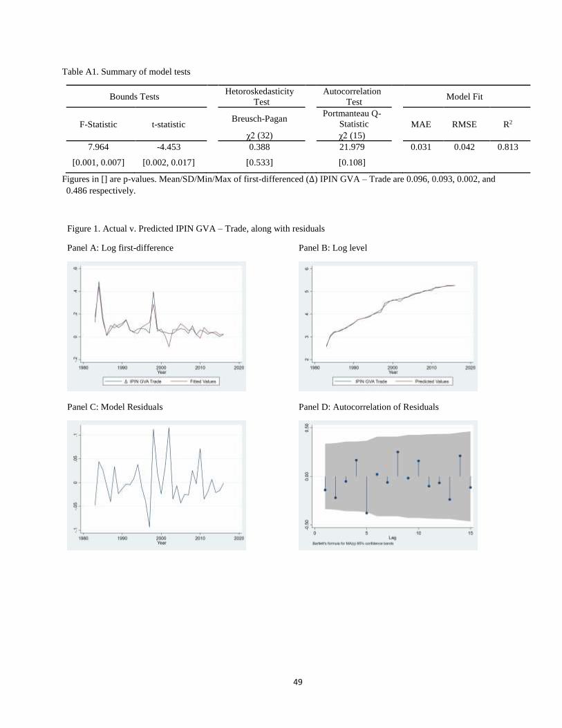
49
Table A1. Summary of model tests
Bounds Tests Hetoroskedasticity
Test Autocorrelation
Test Model Fit
F-Statistic t-statistic Breusch-Pagan Portmanteau Q-
Statistic MAE RMSE R2
χ2 (32) χ2 (15)
7.964 -4.453 0.388 21.979 0.031 0.042 0.813
[0.001, 0.007] [0.002, 0.017] [0.533] [0.108]
Figures in [] are p-values. Mean/SD/Min/Max of first-differenced (∆) IPIN GVA – Trade are 0.096, 0.093, 0.002, and
0.486 respectively.
Figure 1. Actual v. Predicted IPIN GVA – Trade, along with residuals
Panel A: Log first-difference Panel B: Log level
Panel C: Model Residuals Panel D: Autocorrelation of Residuals
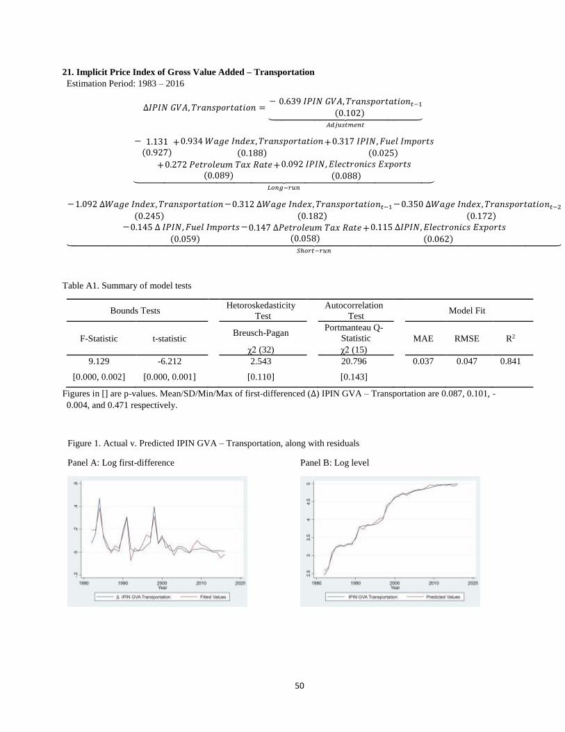
50
21. Implicit Price Index of Gross Value Added – Transportation
Estimation Period: 1983 – 2016
∆𝐼𝑃𝐼𝑁 𝐺𝑉𝐴, 𝑇𝑟𝑎𝑛𝑠𝑝𝑜𝑟𝑡𝑎𝑡𝑖𝑜𝑛 =− 0.639 𝐼𝑃𝐼𝑁 𝐺𝑉𝐴, 𝑇𝑟𝑎𝑛𝑠𝑝𝑜𝑟𝑡𝑎𝑡𝑖𝑜𝑛𝑡−1
(0.102)⏟ 𝐴𝑑𝑗𝑢𝑠𝑡𝑚𝑒𝑛𝑡
− 1.131(0.927)
+0.934 𝑊𝑎𝑔𝑒 𝐼𝑛𝑑𝑒𝑥, 𝑇𝑟𝑎𝑛𝑠𝑝𝑜𝑟𝑡𝑎𝑡𝑖𝑜𝑛
(0.188)+0.317 𝐼𝑃𝐼𝑁, 𝐹𝑢𝑒𝑙 𝐼𝑚𝑝𝑜𝑟𝑡𝑠
(0.025)
+0.272 𝑃𝑒𝑡𝑟𝑜𝑙𝑒𝑢𝑚 𝑇𝑎𝑥 𝑅𝑎𝑡𝑒(0.089)
+0.092 𝐼𝑃𝐼𝑁, 𝐸𝑙𝑒𝑐𝑡𝑟𝑜𝑛𝑖𝑐𝑠 𝐸𝑥𝑝𝑜𝑟𝑡𝑠(0.088)⏟
𝐿𝑜𝑛𝑔−𝑟𝑢𝑛
−1.092 ∆𝑊𝑎𝑔𝑒 𝐼𝑛𝑑𝑒𝑥, 𝑇𝑟𝑎𝑛𝑠𝑝𝑜𝑟𝑡𝑎𝑡𝑖𝑜𝑛
(0.245)
−0.312 ∆𝑊𝑎𝑔𝑒 𝐼𝑛𝑑𝑒𝑥, 𝑇𝑟𝑎𝑛𝑠𝑝𝑜𝑟𝑡𝑎𝑡𝑖𝑜𝑛𝑡−1(0.182)
−0.350 ∆𝑊𝑎𝑔𝑒 𝐼𝑛𝑑𝑒𝑥, 𝑇𝑟𝑎𝑛𝑠𝑝𝑜𝑟𝑡𝑎𝑡𝑖𝑜𝑛𝑡−2(0.172)
−0.145 ∆ 𝐼𝑃𝐼𝑁, 𝐹𝑢𝑒𝑙 𝐼𝑚𝑝𝑜𝑟𝑡𝑠
(0.059)
−0.147 ∆𝑃𝑒𝑡𝑟𝑜𝑙𝑒𝑢𝑚 𝑇𝑎𝑥 𝑅𝑎𝑡𝑒(0.058)
+0.115 ∆𝐼𝑃𝐼𝑁, 𝐸𝑙𝑒𝑐𝑡𝑟𝑜𝑛𝑖𝑐𝑠 𝐸𝑥𝑝𝑜𝑟𝑡𝑠
(0.062)⏟ 𝑆ℎ𝑜𝑟𝑡−𝑟𝑢𝑛
Table A1. Summary of model tests
Bounds Tests Hetoroskedasticity
Test Autocorrelation
Test Model Fit
F-Statistic t-statistic Breusch-Pagan Portmanteau Q-
Statistic MAE RMSE R2
χ2 (32) χ2 (15)
9.129 -6.212 2.543 20.796 0.037 0.047 0.841
[0.000, 0.002] [0.000, 0.001] [0.110] [0.143]
Figures in [] are p-values. Mean/SD/Min/Max of first-differenced (∆) IPIN GVA – Transportation are 0.087, 0.101, -
0.004, and 0.471 respectively.
Figure 1. Actual v. Predicted IPIN GVA – Transportation, along with residuals
Panel A: Log first-difference Panel B: Log level
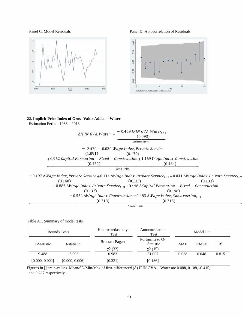
51
Panel C: Model Residuals Panel D: Autocorrelation of Residuals
22. Implicit Price Index of Gross Value Added – Water
Estimation Period: 1983 – 2016
∆𝐼𝑃𝐼𝑁 𝐺𝑉𝐴,𝑊𝑎𝑡𝑒𝑟 =− 0.469 𝐼𝑃𝐼𝑁 𝐺𝑉𝐴,𝑊𝑎𝑡𝑒𝑟𝑡−1
(0.093)⏟ 𝐴𝑑𝑗𝑢𝑠𝑡𝑚𝑒𝑛𝑡
− 2.470(1.091)
+0.030 𝑊𝑎𝑔𝑒 𝐼𝑛𝑑𝑒𝑥, 𝑃𝑟𝑖𝑣𝑎𝑡𝑒 𝑆𝑒𝑟𝑣𝑖𝑐𝑒
(0.179)
+0.962 𝐶𝑎𝑝𝑖𝑡𝑎𝑙 𝐹𝑜𝑟𝑚𝑎𝑡𝑖𝑜𝑛 − 𝐹𝑖𝑥𝑒𝑑 − 𝐶𝑜𝑛𝑠𝑡𝑟𝑢𝑐𝑡𝑖𝑜𝑛(0.122)
+1.169 𝑊𝑎𝑔𝑒 𝐼𝑛𝑑𝑒𝑥, 𝐶𝑜𝑛𝑠𝑡𝑟𝑢𝑐𝑡𝑖𝑜𝑛
(0.464)⏟ 𝐿𝑜𝑛𝑔−𝑟𝑢𝑛
−0.197 ∆𝑊𝑎𝑔𝑒 𝐼𝑛𝑑𝑒𝑥, 𝑃𝑟𝑖𝑣𝑎𝑡𝑒 𝑆𝑒𝑟𝑣𝑖𝑐𝑒
(0.140)+0.114 ∆𝑊𝑎𝑔𝑒 𝐼𝑛𝑑𝑒𝑥, 𝑃𝑟𝑖𝑣𝑎𝑡𝑒 𝑆𝑒𝑟𝑣𝑖𝑐𝑒𝑡−1
(0.133)+0.041 ∆𝑊𝑎𝑔𝑒 𝐼𝑛𝑑𝑒𝑥, 𝑃𝑟𝑖𝑣𝑎𝑡𝑒 𝑆𝑒𝑟𝑣𝑖𝑐𝑒𝑡−2
(0.133)−0.885 ∆𝑊𝑎𝑔𝑒 𝐼𝑛𝑑𝑒𝑥, 𝑃𝑟𝑖𝑣𝑎𝑡𝑒 𝑆𝑒𝑟𝑣𝑖𝑐𝑒𝑡−3
(0.132)
−0.446 ∆𝐶𝑎𝑝𝑖𝑡𝑎𝑙 𝐹𝑜𝑟𝑚𝑎𝑡𝑖𝑜𝑛 − 𝐹𝑖𝑥𝑒𝑑 − 𝐶𝑜𝑛𝑠𝑡𝑟𝑢𝑐𝑡𝑖𝑜𝑛(0.196)
−0.552 ∆𝑊𝑎𝑔𝑒 𝐼𝑛𝑑𝑒𝑥, 𝐶𝑜𝑛𝑠𝑡𝑟𝑢𝑐𝑡𝑖𝑜𝑛
(0.218)
−0.483 ∆𝑊𝑎𝑔𝑒 𝐼𝑛𝑑𝑒𝑥, 𝐶𝑜𝑛𝑠𝑡𝑟𝑢𝑐𝑡𝑖𝑜𝑛𝑡−1(0.215)⏟
𝑆ℎ𝑜𝑟𝑡−𝑟𝑢𝑛
Table A1. Summary of model tests
Bounds Tests Hetoroskedasticity
Test Autocorrelation
Test Model Fit
F-Statistic t-statistic Breusch-Pagan Portmanteau Q-
Statistic MAE RMSE R2
χ2 (32) χ2 (15)
9.488 -5.003 0.983 21.007 0.038 0.048 0.815
[0.000, 0.002] [0.000, 0.006] [0.321] [0.136]
Figures in [] are p-values. Mean/SD/Min/Max of first-differenced (∆) IPIN GVA – Water are 0.088, 0.108, -0.415,
and 0.287 respectively.

52
Figure 1. Actual v. Predicted IPIN GVA – Water, along with residuals
Panel A: Log first-difference Panel B: Log level
Panel C: Model Residuals Panel D: Autocorrelation of Residuals
23. Household Final Consumption Expenditure – Alcohol
Estimation Period: 1981 – 2016
∆𝐻𝐹𝐶𝐸, 𝐴𝑙𝑐𝑜ℎ𝑜𝑙 =− 0.438 𝐻𝐹𝐶𝐸, 𝐴𝑙𝑐𝑜ℎ𝑜𝑙𝑡−1
(0.056)⏟ 𝐴𝑑𝑗𝑢𝑠𝑡𝑚𝑒𝑛𝑡
− 2.610(1.027)
−1.356 𝐼𝑃𝐼𝑁 𝐻𝐹𝐶𝐸, 𝐴𝑙𝑐𝑜ℎ𝑜𝑙(0.119)
+0.586 𝑁𝑒𝑡 𝐷𝑖𝑠𝑝𝑜𝑠𝑎𝑏𝑙𝑒 𝐼𝑛𝑐𝑜𝑚𝑒(0.119)
+1.301 𝐻𝐹𝐶𝐸, 𝑇𝑜𝑏𝑎𝑐𝑐𝑜(0.350)⏟
𝐿𝑜𝑛𝑔−𝑟𝑢𝑛
+0.135 ∆𝐼𝑃𝐼𝑁 𝐻𝐹𝐶𝐸, 𝐴𝑙𝑐𝑜ℎ𝑜𝑙𝑡−1(0.189)
+0.343 ∆𝐼𝑃𝐼𝑁 𝐻𝐹𝐶𝐸, 𝐴𝑙𝑐𝑜ℎ𝑜𝑙𝑡−2(0.179)
−0.529 ∆𝐻𝐹𝐶𝐸, 𝑇𝑜𝑏𝑎𝑐𝑐𝑜(0.281)
−0.759 ∆𝐻𝐹𝐶𝐸, 𝑇𝑜𝑏𝑎𝑐𝑐𝑜𝑡−1(0.353)
−0.780 ∆𝐻𝐹𝐶𝐸, 𝑇𝑜𝑏𝑎𝑐𝑐𝑜𝑡−2(0.289)
−0.766 ∆𝐻𝐹𝐶𝐸, 𝑇𝑜𝑏𝑎𝑐𝑐𝑜𝑡−3(0.285)⏟
𝑆ℎ𝑜𝑟𝑡−𝑟𝑢𝑛
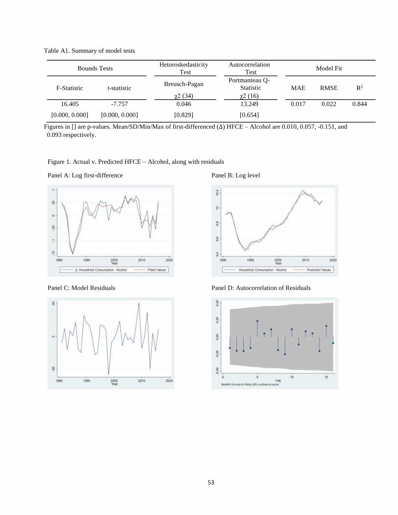
53
Table A1. Summary of model tests
Bounds Tests Hetoroskedasticity
Test Autocorrelation
Test Model Fit
F-Statistic t-statistic Breusch-Pagan Portmanteau Q-
Statistic MAE RMSE R2
χ2 (34) χ2 (16)
16.405 -7.757 0.046 13.249 0.017 0.022 0.844
[0.000, 0.000] [0.000, 0.000] [0.829] [0.654]
Figures in [] are p-values. Mean/SD/Min/Max of first-differenced (∆) HFCE – Alcohol are 0.010, 0.057, -0.151, and
0.093 respectively.
Figure 1. Actual v. Predicted HFCE – Alcohol, along with residuals
Panel A: Log first-difference Panel B: Log level
Panel C: Model Residuals Panel D: Autocorrelation of Residuals
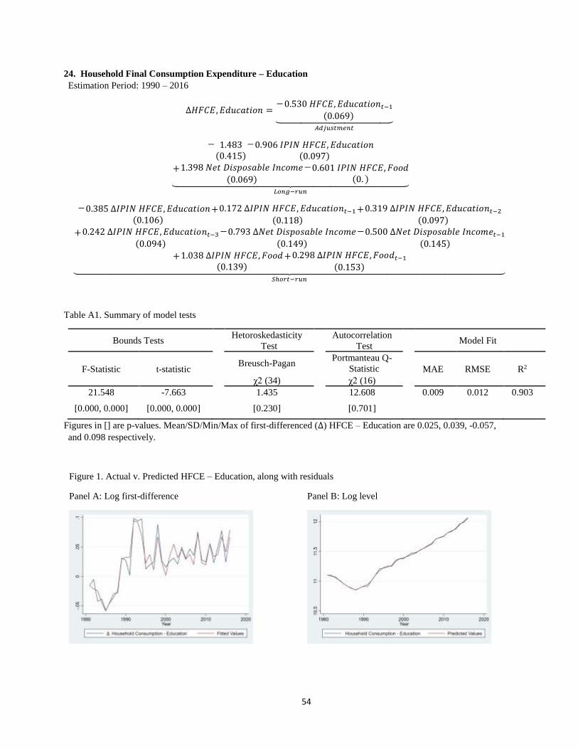
54
24. Household Final Consumption Expenditure – Education
Estimation Period: 1990 – 2016
∆𝐻𝐹𝐶𝐸, 𝐸𝑑𝑢𝑐𝑎𝑡𝑖𝑜𝑛 =−0.530 𝐻𝐹𝐶𝐸, 𝐸𝑑𝑢𝑐𝑎𝑡𝑖𝑜𝑛𝑡−1
(0.069)⏟ 𝐴𝑑𝑗𝑢𝑠𝑡𝑚𝑒𝑛𝑡
− 1.483(0.415)
−0.906 𝐼𝑃𝐼𝑁 𝐻𝐹𝐶𝐸, 𝐸𝑑𝑢𝑐𝑎𝑡𝑖𝑜𝑛(0.097)
+1.398 𝑁𝑒𝑡 𝐷𝑖𝑠𝑝𝑜𝑠𝑎𝑏𝑙𝑒 𝐼𝑛𝑐𝑜𝑚𝑒(0.069)
−0.601 𝐼𝑃𝐼𝑁 𝐻𝐹𝐶𝐸, 𝐹𝑜𝑜𝑑(0. )⏟
𝐿𝑜𝑛𝑔−𝑟𝑢𝑛
−0.385 ∆𝐼𝑃𝐼𝑁 𝐻𝐹𝐶𝐸, 𝐸𝑑𝑢𝑐𝑎𝑡𝑖𝑜𝑛(0.106)
+0.172 ∆𝐼𝑃𝐼𝑁 𝐻𝐹𝐶𝐸, 𝐸𝑑𝑢𝑐𝑎𝑡𝑖𝑜𝑛𝑡−1(0.118)
+0.319 ∆𝐼𝑃𝐼𝑁 𝐻𝐹𝐶𝐸, 𝐸𝑑𝑢𝑐𝑎𝑡𝑖𝑜𝑛𝑡−2(0.097)
+0.242 ∆𝐼𝑃𝐼𝑁 𝐻𝐹𝐶𝐸, 𝐸𝑑𝑢𝑐𝑎𝑡𝑖𝑜𝑛𝑡−3(0.094)
−0.793 ∆𝑁𝑒𝑡 𝐷𝑖𝑠𝑝𝑜𝑠𝑎𝑏𝑙𝑒 𝐼𝑛𝑐𝑜𝑚𝑒(0.149)
−0.500 ∆𝑁𝑒𝑡 𝐷𝑖𝑠𝑝𝑜𝑠𝑎𝑏𝑙𝑒 𝐼𝑛𝑐𝑜𝑚𝑒𝑡−1(0.145)
+1.038 ∆𝐼𝑃𝐼𝑁 𝐻𝐹𝐶𝐸, 𝐹𝑜𝑜𝑑(0.139)
+0.298 ∆𝐼𝑃𝐼𝑁 𝐻𝐹𝐶𝐸, 𝐹𝑜𝑜𝑑𝑡−1(0.153)⏟
𝑆ℎ𝑜𝑟𝑡−𝑟𝑢𝑛
Table A1. Summary of model tests
Bounds Tests Hetoroskedasticity
Test Autocorrelation
Test Model Fit
F-Statistic t-statistic Breusch-Pagan Portmanteau Q-
Statistic MAE RMSE R2
χ2 (34) χ2 (16)
21.548 -7.663 1.435 12.608 0.009 0.012 0.903
[0.000, 0.000] [0.000, 0.000] [0.230] [0.701]
Figures in [] are p-values. Mean/SD/Min/Max of first-differenced (∆) HFCE – Education are 0.025, 0.039, -0.057,
and 0.098 respectively.
Figure 1. Actual v. Predicted HFCE – Education, along with residuals
Panel A: Log first-difference Panel B: Log level
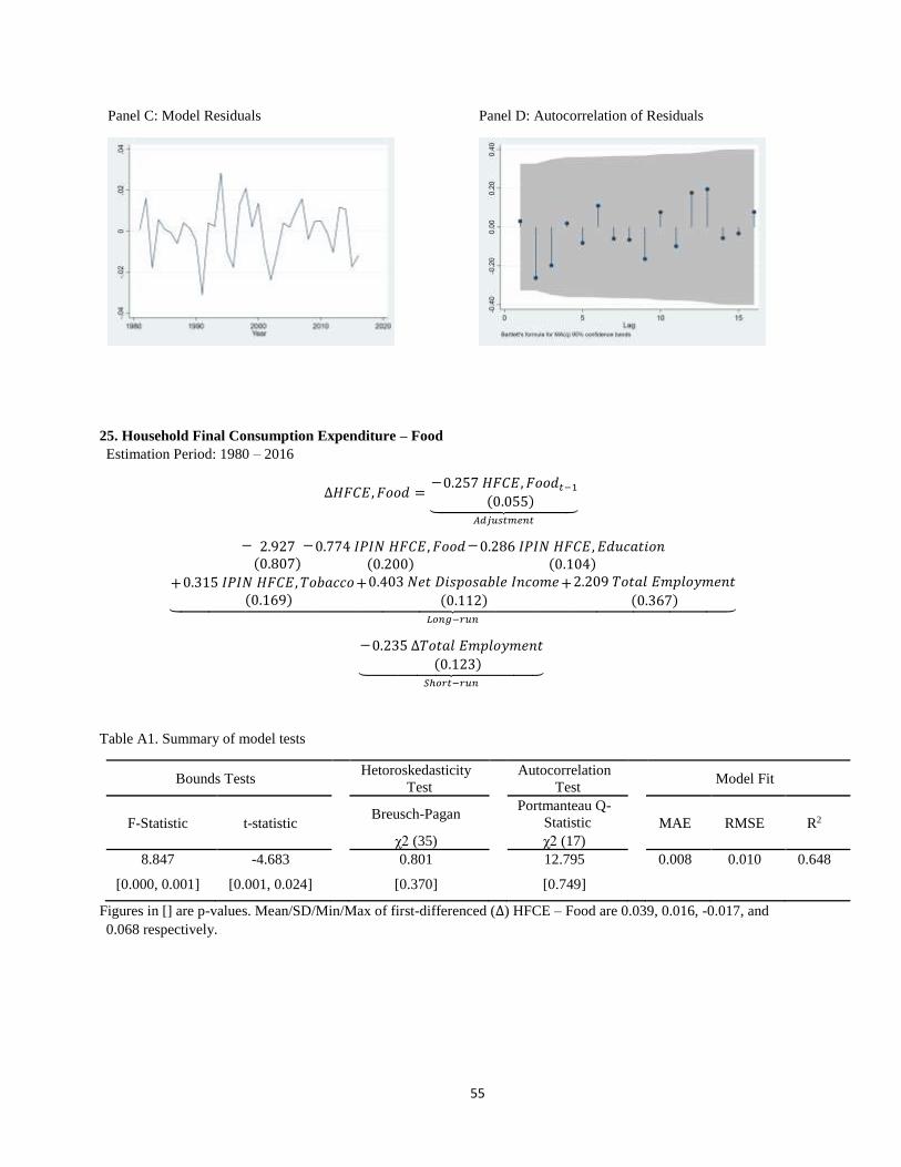
55
Panel C: Model Residuals Panel D: Autocorrelation of Residuals
25. Household Final Consumption Expenditure – Food
Estimation Period: 1980 – 2016
∆𝐻𝐹𝐶𝐸, 𝐹𝑜𝑜𝑑 =−0.257 𝐻𝐹𝐶𝐸, 𝐹𝑜𝑜𝑑𝑡−1
(0.055)⏟ 𝐴𝑑𝑗𝑢𝑠𝑡𝑚𝑒𝑛𝑡
− 2.927(0.807)
−0.774 𝐼𝑃𝐼𝑁 𝐻𝐹𝐶𝐸, 𝐹𝑜𝑜𝑑(0.200)
−0.286 𝐼𝑃𝐼𝑁 𝐻𝐹𝐶𝐸, 𝐸𝑑𝑢𝑐𝑎𝑡𝑖𝑜𝑛(0.104)
+0.315 𝐼𝑃𝐼𝑁 𝐻𝐹𝐶𝐸, 𝑇𝑜𝑏𝑎𝑐𝑐𝑜(0.169)
+0.403 𝑁𝑒𝑡 𝐷𝑖𝑠𝑝𝑜𝑠𝑎𝑏𝑙𝑒 𝐼𝑛𝑐𝑜𝑚𝑒(0.112)
+2.209 𝑇𝑜𝑡𝑎𝑙 𝐸𝑚𝑝𝑙𝑜𝑦𝑚𝑒𝑛𝑡
(0.367)⏟ 𝐿𝑜𝑛𝑔−𝑟𝑢𝑛
−0.235 ∆𝑇𝑜𝑡𝑎𝑙 𝐸𝑚𝑝𝑙𝑜𝑦𝑚𝑒𝑛𝑡(0.123)⏟
𝑆ℎ𝑜𝑟𝑡−𝑟𝑢𝑛
Table A1. Summary of model tests
Bounds Tests Hetoroskedasticity
Test Autocorrelation
Test Model Fit
F-Statistic t-statistic Breusch-Pagan Portmanteau Q-
Statistic MAE RMSE R2
χ2 (35) χ2 (17)
8.847 -4.683 0.801 12.795 0.008 0.010 0.648
[0.000, 0.001] [0.001, 0.024] [0.370] [0.749]
Figures in [] are p-values. Mean/SD/Min/Max of first-differenced (∆) HFCE – Food are 0.039, 0.016, -0.017, and
0.068 respectively.

56
Figure 1. Actual v. Predicted HFCE – Food, along with residuals
Panel A: Log first-difference Panel B: Log level
Panel C: Model Residuals Panel D: Autocorrelation of Residuals
26. Household Final Consumption Expenditure – Medical
Estimation Period: 1979 – 2016
∆𝐻𝐹𝐶𝐸,𝑀𝑒𝑑𝑖𝑐𝑎𝑙 =− 0.297 𝐻𝐹𝐶𝐸,𝑀𝑒𝑑𝑖𝑐𝑎𝑙𝑡−1
(0.070)⏟ 𝐴𝑑𝑗𝑢𝑠𝑡𝑚𝑒𝑛𝑡
− 0.418(0.445)
−2.852 𝐼𝑃𝐼𝑁 𝐻𝐹𝐶𝐸,𝑀𝑒𝑑𝑖𝑐𝑎𝑙(0.286)
+1.248 𝑁𝑒𝑡 𝐷𝑖𝑠𝑝𝑜𝑠𝑎𝑏𝑙𝑒 𝐼𝑛𝑐𝑜𝑚𝑒(0.151)
+1.452 𝐼𝑃𝐼𝑁 𝐻𝐹𝐶𝐸, 𝐸𝑑𝑢𝑐𝑎𝑡𝑖𝑜𝑛(0.362)⏟
𝐿𝑜𝑛𝑔−𝑟𝑢𝑛
+0.447 ∆𝐻𝐹𝐶𝐸,𝑀𝑒𝑑𝑖𝑐𝑎𝑙𝑡−1(0.130)
+0.082 ∆𝐼𝑃𝐼𝑁 𝐻𝐹𝐶𝐸,𝑀𝑒𝑑𝑖𝑐𝑎𝑙(0.407)
+0.592 ∆𝐼𝑃𝐼𝑁 𝐻𝐹𝐶𝐸,𝑀𝑒𝑑𝑖𝑐𝑎𝑙𝑡−1(0.347)
−0.198 ∆𝑁𝑒𝑡 𝐷𝑖𝑠𝑝𝑜𝑠𝑎𝑏𝑙𝑒 𝐼𝑛𝑐𝑜𝑚𝑒(0.174)
−0.343 ∆𝑁𝑒𝑡 𝐷𝑖𝑠𝑝𝑜𝑠𝑎𝑏𝑙𝑒 𝐼𝑛𝑐𝑜𝑚𝑒𝑡−1(0.179)
−0.090 ∆𝐼𝑃𝐼𝑁 𝐻𝐹𝐶𝐸, 𝐸𝑑𝑢𝑐𝑎𝑡𝑖𝑜𝑛(0.351)
−0.320 ∆𝐼𝑃𝐼𝑁 𝐻𝐹𝐶𝐸, 𝐸𝑑𝑢𝑐𝑎𝑡𝑖𝑜𝑛𝑡−1(0. )⏟
𝑆ℎ𝑜𝑟𝑡−𝑟𝑢𝑛

57
Table A1. Summary of model tests
Bounds Tests Hetoroskedasticity
Test Autocorrelation
Test Model Fit
F-Statistic t-statistic Breusch-Pagan Portmanteau Q-
Statistic MAE RMSE R2
χ2 (36) χ2 (17)
4.901 -4.201 0.204 18.468 0.014 0.019 0.829
[0.012, 0.054] [0.003, 0.025] [0.650] [0.359]
Figures in [] are p-values. Mean/SD/Min/Max of first-differenced (∆) HFCE – Medical are 0.031, 0.047, -0.063, and
0.111 respectively.
Figure 1. Actual v. Predicted HFCE – Medical, along with residuals
Panel A: Log first-difference Panel B: Log level
Panel C: Model Residuals Panel D: Autocorrelation of Residuals

58
27. Household Final Consumption Expenditure – Housing
Estimation Period: 1981 – 2016
∆𝐻𝐹𝐶𝐸,𝐻𝑜𝑢𝑠𝑖𝑛𝑔 =−1.401 𝐻𝐹𝐶𝐸,𝐻𝑜𝑢𝑠𝑖𝑛𝑔𝑡−1
(0.208)⏟ 𝐴𝑑𝑗𝑢𝑠𝑡𝑚𝑒𝑛𝑡
+ 12.222(1.841)
+0.500 𝐼𝑃𝐼𝑁 𝐻𝐹𝐶𝐸,𝐻𝑜𝑢𝑠𝑖𝑛𝑔
(0.071)+0.227 𝑁𝑒𝑡 𝐷𝑖𝑠𝑝𝑜𝑠𝑎𝑏𝑙𝑒 𝐼𝑛𝑐𝑜𝑚𝑒
(0.029)−0.476 𝐼𝑃𝐼𝑁 𝐺𝑉𝐴,𝑀𝑎𝑛𝑢𝑓𝑎𝑐𝑡𝑢𝑟𝑖𝑛𝑔
(0.042)
−0.049 𝐼𝑃𝐼𝑁,𝑀𝑎𝑡𝑒𝑟𝑖𝑎𝑙𝑠 𝐼𝑚𝑝𝑜𝑟𝑡𝑠
(0.010)⏟ 𝐿𝑜𝑛𝑔−𝑟𝑢𝑛
−0.718 ∆𝐼𝑃𝐼𝑁 𝐻𝐹𝐶𝐸,𝐻𝑜𝑢𝑠𝑖𝑛𝑔
(0.157)
−0.532 ∆𝐼𝑃𝐼𝑁 𝐻𝐹𝐶𝐸,𝐻𝑜𝑢𝑠𝑖𝑛𝑔𝑡−1(0.116)
−0.338 ∆𝐼𝑃𝐼𝑁 𝐻𝐹𝐶𝐸,𝐻𝑜𝑢𝑠𝑖𝑛𝑔𝑡−2(0.108)
−0.085 ∆𝐼𝑃𝐼𝑁 𝐻𝐹𝐶𝐸,𝐻𝑜𝑢𝑠𝑖𝑛𝑔𝑡−3(0.047)
+0.601 ∆𝐼𝑃𝐼𝑁 𝐺𝑉𝐴,𝑀𝑎𝑛𝑢𝑓𝑎𝑐𝑡𝑢𝑟𝑖𝑛𝑔
(0.131)
+0.386 ∆𝐼𝑃𝐼𝑁 𝐺𝑉𝐴,𝑀𝑎𝑛𝑢𝑓𝑎𝑐𝑡𝑢𝑟𝑖𝑛𝑔𝑡−1(0.095)
+0.250 ∆𝐼𝑃𝐼𝑁 𝐺𝑉𝐴,𝑀𝑎𝑛𝑢𝑓𝑎𝑐𝑡𝑢𝑟𝑖𝑛𝑔𝑡−2(0.085)⏟
𝑆ℎ𝑜𝑟𝑡−𝑟𝑢𝑛
Table A1. Summary of model tests
Bounds Tests Hetoroskedasticity
Test Autocorrelation
Test Model Fit
F-Statistic t-statistic Breusch-Pagan Portmanteau Q-
Statistic MAE RMSE R2
χ2 (34) χ2 (16)
10.604 -6.734 0.427 11.274 0.006 0.008 0.780
[0.000, 0.001] [0.000, 0.000] [0.512] [0.792]
Figures in [] are p-values. Mean/SD/Min/Max of first-differenced (∆) HFCE – Housing are 0.036, 0.019, -0.008, and
0.074 respectively.
Figure 1. Actual v. Predicted HFCE – Housing, along with residuals
Panel A: Log first-difference Panel B: Log level

59
Panel C: Model Residuals Panel D: Autocorrelation of Residuals
28. Household Final Consumption Expenditure – Non-alcoholic Beverages
Estimation Period: 1981 – 2016
∆𝐻𝐹𝐶𝐸,𝑁𝑜𝑛 − 𝑎𝑙𝑐𝑜ℎ𝑜𝑙 =−0.355 𝐻𝐹𝐶𝐸,𝑁𝑜𝑛 − 𝑎𝑙𝑐𝑜ℎ𝑜𝑙𝑡−1
(0.085)⏟ 𝐴𝑑𝑗𝑢𝑠𝑡𝑚𝑒𝑛𝑡
+ 0.855(0.433)
−0.242 𝐼𝑃𝐼𝑁 𝐻𝐹𝐶𝐸,𝑁𝑜𝑛 − 𝑎𝑙𝑐𝑜ℎ𝑜𝑙(0.150)
+0.350 𝑁𝑒𝑡 𝐷𝑖𝑠𝑝𝑜𝑠𝑎𝑏𝑙𝑒 𝐼𝑛𝑐𝑜𝑚𝑒
(0.042)−0.891 𝑆ℎ𝑎𝑟𝑒 𝑜𝑓 𝐶𝑃𝐼, 𝐴𝑙𝑐𝑜ℎ𝑜𝑙
(0.289)
−0.266 𝑂𝑝𝑒𝑛𝑛𝑒𝑠𝑠(0.061)⏟
𝐿𝑜𝑛𝑔−𝑟𝑢𝑛
+0.472 ∆𝐻𝐹𝐶𝐸,𝑁𝑜𝑛 − 𝑎𝑙𝑐𝑜ℎ𝑜𝑙(0.120)
+0.238 ∆𝐻𝐹𝐶𝐸,𝑁𝑜𝑛 − 𝑎𝑙𝑐𝑜ℎ𝑜𝑙(0.140)
−0.252 ∆𝐻𝐹𝐶𝐸,𝑁𝑜𝑛 − 𝑎𝑙𝑐𝑜ℎ𝑜𝑙(0.148)
+0.187 ∆𝐼𝑃𝐼𝑁 𝐻𝐹𝐶𝐸,𝑁𝑜𝑛 − 𝑎𝑙𝑐𝑜ℎ𝑜𝑙(0.076)⏟
𝑆ℎ𝑜𝑟𝑡−𝑟𝑢𝑛
Table A1. Summary of model tests
Bounds Tests Hetoroskedasticity
Test Autocorrelation
Test Model Fit
F-Statistic t-statistic Breusch-Pagan Portmanteau Q-
Statistic MAE RMSE R2
χ2 (34) χ2 (16)
9.506 -4.149 1.160 12.793 0.013 0.015 0.838
[0.000, 0.001] [0.003, 9.506] [0.281] [0.687]
Figures in [] are p-values. Mean/SD/Min/Max of first-differenced (∆) HFCE – Non-alcoholic Beverages are 0.057,
0.039, -0.020, and 0.142 respectively.
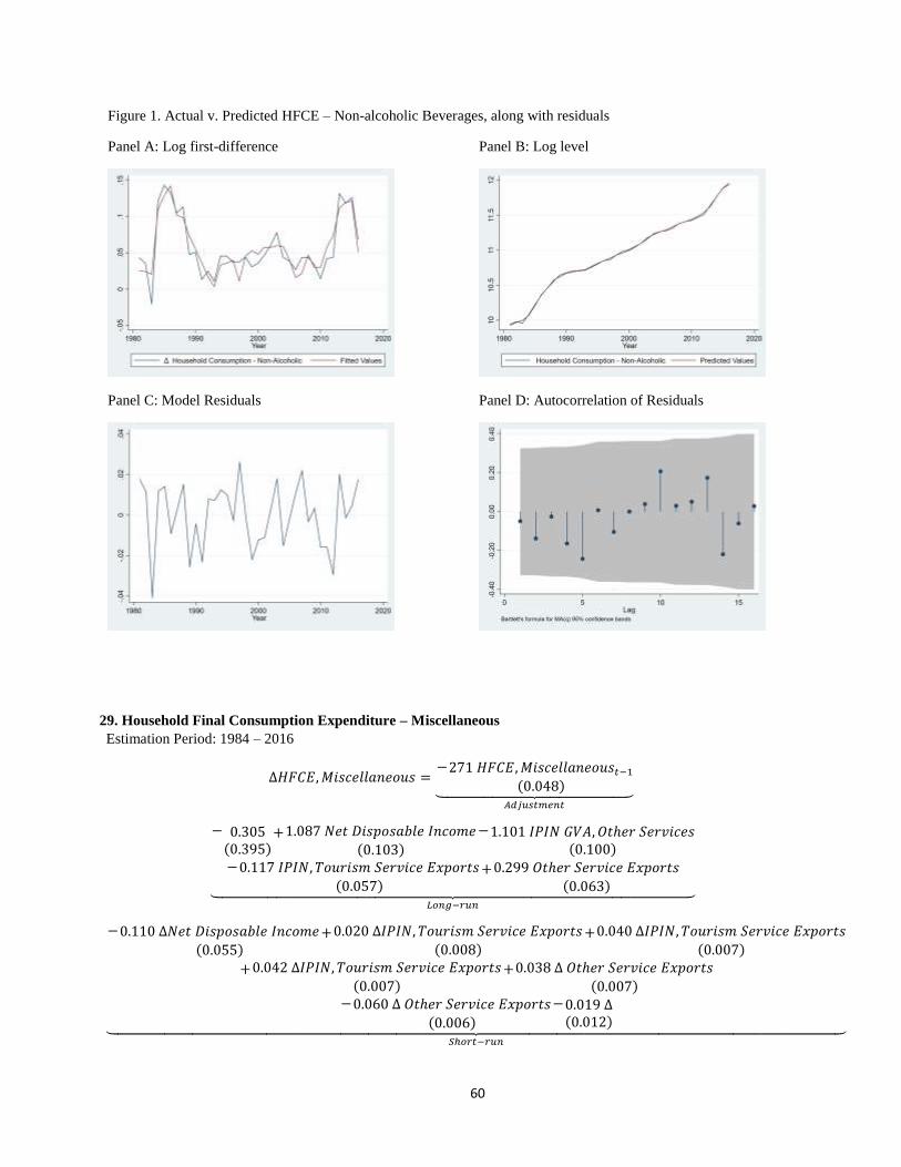
60
Figure 1. Actual v. Predicted HFCE – Non-alcoholic Beverages, along with residuals
Panel A: Log first-difference Panel B: Log level
Panel C: Model Residuals Panel D: Autocorrelation of Residuals
29. Household Final Consumption Expenditure – Miscellaneous
Estimation Period: 1984 – 2016
∆𝐻𝐹𝐶𝐸,𝑀𝑖𝑠𝑐𝑒𝑙𝑙𝑎𝑛𝑒𝑜𝑢𝑠 =−271 𝐻𝐹𝐶𝐸,𝑀𝑖𝑠𝑐𝑒𝑙𝑙𝑎𝑛𝑒𝑜𝑢𝑠𝑡−1
(0.048)⏟ 𝐴𝑑𝑗𝑢𝑠𝑡𝑚𝑒𝑛𝑡
− 0.305(0.395)
+1.087 𝑁𝑒𝑡 𝐷𝑖𝑠𝑝𝑜𝑠𝑎𝑏𝑙𝑒 𝐼𝑛𝑐𝑜𝑚𝑒(0.103)
−1.101 𝐼𝑃𝐼𝑁 𝐺𝑉𝐴, 𝑂𝑡ℎ𝑒𝑟 𝑆𝑒𝑟𝑣𝑖𝑐𝑒𝑠(0.100)
−0.117 𝐼𝑃𝐼𝑁, 𝑇𝑜𝑢𝑟𝑖𝑠𝑚 𝑆𝑒𝑟𝑣𝑖𝑐𝑒 𝐸𝑥𝑝𝑜𝑟𝑡𝑠(0.057)
+0.299 𝑂𝑡ℎ𝑒𝑟 𝑆𝑒𝑟𝑣𝑖𝑐𝑒 𝐸𝑥𝑝𝑜𝑟𝑡𝑠(0.063)⏟
𝐿𝑜𝑛𝑔−𝑟𝑢𝑛
−0.110 ∆𝑁𝑒𝑡 𝐷𝑖𝑠𝑝𝑜𝑠𝑎𝑏𝑙𝑒 𝐼𝑛𝑐𝑜𝑚𝑒(0.055)
+0.020 ∆𝐼𝑃𝐼𝑁, 𝑇𝑜𝑢𝑟𝑖𝑠𝑚 𝑆𝑒𝑟𝑣𝑖𝑐𝑒 𝐸𝑥𝑝𝑜𝑟𝑡𝑠(0.008)
+0.040 ∆𝐼𝑃𝐼𝑁, 𝑇𝑜𝑢𝑟𝑖𝑠𝑚 𝑆𝑒𝑟𝑣𝑖𝑐𝑒 𝐸𝑥𝑝𝑜𝑟𝑡𝑠(0.007)
+0.042 ∆𝐼𝑃𝐼𝑁, 𝑇𝑜𝑢𝑟𝑖𝑠𝑚 𝑆𝑒𝑟𝑣𝑖𝑐𝑒 𝐸𝑥𝑝𝑜𝑟𝑡𝑠(0.007)
+0.038 ∆ 𝑂𝑡ℎ𝑒𝑟 𝑆𝑒𝑟𝑣𝑖𝑐𝑒 𝐸𝑥𝑝𝑜𝑟𝑡𝑠(0.007)
−0.060 ∆ 𝑂𝑡ℎ𝑒𝑟 𝑆𝑒𝑟𝑣𝑖𝑐𝑒 𝐸𝑥𝑝𝑜𝑟𝑡𝑠(0.006)
−0.019 ∆(0.012)⏟
𝑆ℎ𝑜𝑟𝑡−𝑟𝑢𝑛
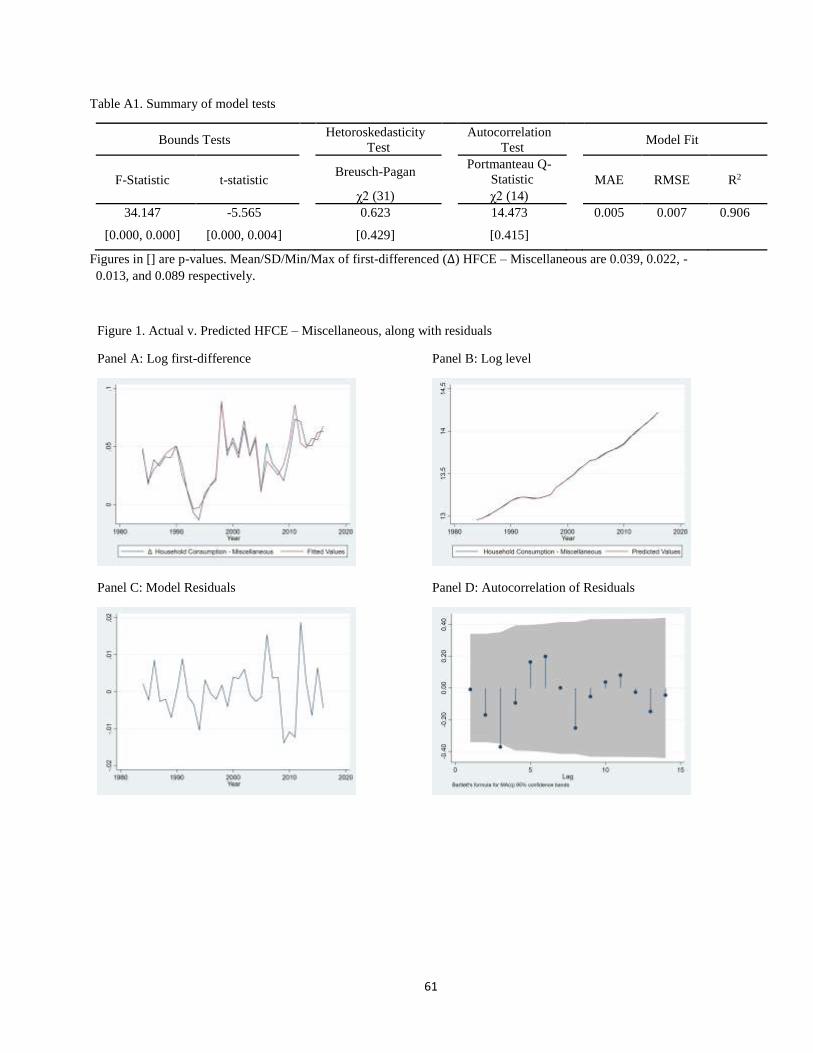
61
Table A1. Summary of model tests
Bounds Tests Hetoroskedasticity
Test Autocorrelation
Test Model Fit
F-Statistic t-statistic Breusch-Pagan Portmanteau Q-
Statistic MAE RMSE R2
χ2 (31) χ2 (14)
34.147 -5.565 0.623 14.473 0.005 0.007 0.906
[0.000, 0.000] [0.000, 0.004] [0.429] [0.415]
Figures in [] are p-values. Mean/SD/Min/Max of first-differenced (∆) HFCE – Miscellaneous are 0.039, 0.022, -
0.013, and 0.089 respectively.
Figure 1. Actual v. Predicted HFCE – Miscellaneous, along with residuals
Panel A: Log first-difference Panel B: Log level
Panel C: Model Residuals Panel D: Autocorrelation of Residuals
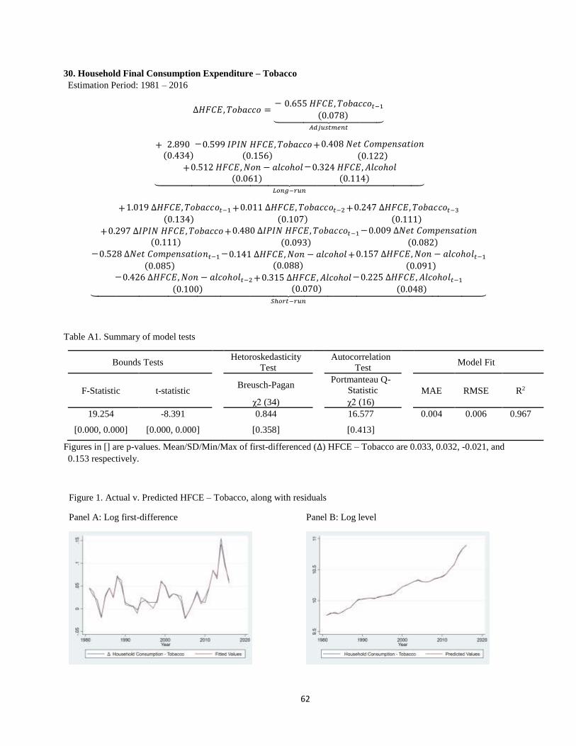
62
30. Household Final Consumption Expenditure – Tobacco
Estimation Period: 1981 – 2016
∆𝐻𝐹𝐶𝐸, 𝑇𝑜𝑏𝑎𝑐𝑐𝑜 =− 0.655 𝐻𝐹𝐶𝐸, 𝑇𝑜𝑏𝑎𝑐𝑐𝑜𝑡−1
(0.078)⏟ 𝐴𝑑𝑗𝑢𝑠𝑡𝑚𝑒𝑛𝑡
+ 2.890(0.434)
−0.599 𝐼𝑃𝐼𝑁 𝐻𝐹𝐶𝐸, 𝑇𝑜𝑏𝑎𝑐𝑐𝑜(0.156)
+0.408 𝑁𝑒𝑡 𝐶𝑜𝑚𝑝𝑒𝑛𝑠𝑎𝑡𝑖𝑜𝑛(0.122)
+0.512 𝐻𝐹𝐶𝐸,𝑁𝑜𝑛 − 𝑎𝑙𝑐𝑜ℎ𝑜𝑙(0.061)
−0.324 𝐻𝐹𝐶𝐸, 𝐴𝑙𝑐𝑜ℎ𝑜𝑙(0.114)⏟
𝐿𝑜𝑛𝑔−𝑟𝑢𝑛
+1.019 ∆𝐻𝐹𝐶𝐸, 𝑇𝑜𝑏𝑎𝑐𝑐𝑜𝑡−1(0.134)
+0.011 ∆𝐻𝐹𝐶𝐸, 𝑇𝑜𝑏𝑎𝑐𝑐𝑜𝑡−2(0.107)
+0.247 ∆𝐻𝐹𝐶𝐸, 𝑇𝑜𝑏𝑎𝑐𝑐𝑜𝑡−3(0.111)
+0.297 ∆𝐼𝑃𝐼𝑁 𝐻𝐹𝐶𝐸, 𝑇𝑜𝑏𝑎𝑐𝑐𝑜(0.111)
+0.480 ∆𝐼𝑃𝐼𝑁 𝐻𝐹𝐶𝐸, 𝑇𝑜𝑏𝑎𝑐𝑐𝑜𝑡−1(0.093)
−0.009 ∆𝑁𝑒𝑡 𝐶𝑜𝑚𝑝𝑒𝑛𝑠𝑎𝑡𝑖𝑜𝑛(0.082)
−0.528 ∆𝑁𝑒𝑡 𝐶𝑜𝑚𝑝𝑒𝑛𝑠𝑎𝑡𝑖𝑜𝑛𝑡−1(0.085)
−0.141 ∆𝐻𝐹𝐶𝐸,𝑁𝑜𝑛 − 𝑎𝑙𝑐𝑜ℎ𝑜𝑙(0.088)
+0.157 ∆𝐻𝐹𝐶𝐸,𝑁𝑜𝑛 − 𝑎𝑙𝑐𝑜ℎ𝑜𝑙𝑡−1(0.091)
−0.426 ∆𝐻𝐹𝐶𝐸,𝑁𝑜𝑛 − 𝑎𝑙𝑐𝑜ℎ𝑜𝑙𝑡−2(0.100)
+0.315 ∆𝐻𝐹𝐶𝐸, 𝐴𝑙𝑐𝑜ℎ𝑜𝑙(0.070)
−0.225 ∆𝐻𝐹𝐶𝐸, 𝐴𝑙𝑐𝑜ℎ𝑜𝑙𝑡−1(0.048)⏟
𝑆ℎ𝑜𝑟𝑡−𝑟𝑢𝑛
Table A1. Summary of model tests
Bounds Tests Hetoroskedasticity
Test Autocorrelation
Test Model Fit
F-Statistic t-statistic Breusch-Pagan Portmanteau Q-
Statistic MAE RMSE R2
χ2 (34) χ2 (16)
19.254 -8.391 0.844 16.577 0.004 0.006 0.967
[0.000, 0.000] [0.000, 0.000] [0.358] [0.413]
Figures in [] are p-values. Mean/SD/Min/Max of first-differenced (∆) HFCE – Tobacco are 0.033, 0.032, -0.021, and
0.153 respectively.
Figure 1. Actual v. Predicted HFCE – Tobacco, along with residuals
Panel A: Log first-difference Panel B: Log level
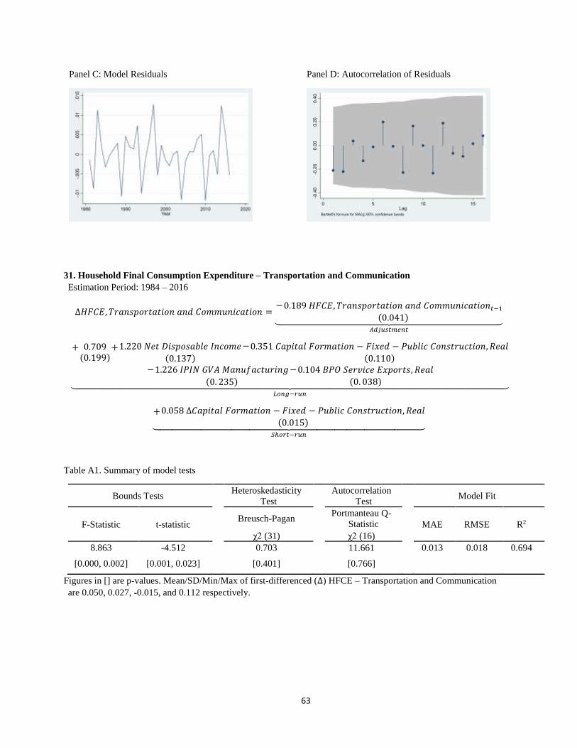
63
Panel C: Model Residuals Panel D: Autocorrelation of Residuals
31. Household Final Consumption Expenditure – Transportation and Communication
Estimation Period: 1984 – 2016
∆𝐻𝐹𝐶𝐸, 𝑇𝑟𝑎𝑛𝑠𝑝𝑜𝑟𝑡𝑎𝑡𝑖𝑜𝑛 𝑎𝑛𝑑 𝐶𝑜𝑚𝑚𝑢𝑛𝑖𝑐𝑎𝑡𝑖𝑜𝑛 =−0.189 𝐻𝐹𝐶𝐸, 𝑇𝑟𝑎𝑛𝑠𝑝𝑜𝑟𝑡𝑎𝑡𝑖𝑜𝑛 𝑎𝑛𝑑 𝐶𝑜𝑚𝑚𝑢𝑛𝑖𝑐𝑎𝑡𝑖𝑜𝑛𝑡−1
(0.041)⏟ 𝐴𝑑𝑗𝑢𝑠𝑡𝑚𝑒𝑛𝑡
+ 0.709(0.199)
+1.220 𝑁𝑒𝑡 𝐷𝑖𝑠𝑝𝑜𝑠𝑎𝑏𝑙𝑒 𝐼𝑛𝑐𝑜𝑚𝑒
(0.137)
−0.351 𝐶𝑎𝑝𝑖𝑡𝑎𝑙 𝐹𝑜𝑟𝑚𝑎𝑡𝑖𝑜𝑛 − 𝐹𝑖𝑥𝑒𝑑 − 𝑃𝑢𝑏𝑙𝑖𝑐 𝐶𝑜𝑛𝑠𝑡𝑟𝑢𝑐𝑡𝑖𝑜𝑛, 𝑅𝑒𝑎𝑙
(0.110)−1.226 𝐼𝑃𝐼𝑁 𝐺𝑉𝐴 𝑀𝑎𝑛𝑢𝑓𝑎𝑐𝑡𝑢𝑟𝑖𝑛𝑔
(0. 235)
−0.104 𝐵𝑃𝑂 𝑆𝑒𝑟𝑣𝑖𝑐𝑒 𝐸𝑥𝑝𝑜𝑟𝑡𝑠, 𝑅𝑒𝑎𝑙(0. 038)⏟
𝐿𝑜𝑛𝑔−𝑟𝑢𝑛
+0.058 ∆𝐶𝑎𝑝𝑖𝑡𝑎𝑙 𝐹𝑜𝑟𝑚𝑎𝑡𝑖𝑜𝑛 − 𝐹𝑖𝑥𝑒𝑑 − 𝑃𝑢𝑏𝑙𝑖𝑐 𝐶𝑜𝑛𝑠𝑡𝑟𝑢𝑐𝑡𝑖𝑜𝑛, 𝑅𝑒𝑎𝑙(0.015)⏟
𝑆ℎ𝑜𝑟𝑡−𝑟𝑢𝑛
Table A1. Summary of model tests
Bounds Tests Heteroskedasticity
Test Autocorrelation
Test Model Fit
F-Statistic t-statistic Breusch-Pagan Portmanteau Q-
Statistic MAE RMSE R2
χ2 (31) χ2 (16)
8.863 -4.512 0.703 11.661 0.013 0.018 0.694
[0.000, 0.002] [0.001, 0.023] [0.401] [0.766]
Figures in [] are p-values. Mean/SD/Min/Max of first-differenced (∆) HFCE – Transportation and Communication
are 0.050, 0.027, -0.015, and 0.112 respectively.

64
Figure 1. Actual v. Predicted HFCE – Transportation and Communication, along with residuals
Panel A: Log first-difference Panel B: Log level
Panel C: Model Residuals Panel D: Autocorrelation of Residuals
32. Household Final Consumption Expenditure – Utilities
Estimation Period: 1983 – 2016
∆𝐻𝐹𝐶𝐸, 𝑈𝑡𝑖𝑙𝑖𝑡𝑖𝑒𝑠 =−0.645 𝐻𝐹𝐶𝐸, 𝑈𝑡𝑖𝑙𝑖𝑡𝑖𝑒𝑠𝑡−1
(0.176)⏟ 𝐴𝑑𝑗𝑢𝑠𝑡𝑚𝑒𝑛𝑡
− 30.487(12.926)
−0.339 𝐼𝑃𝐼𝑁 𝐻𝐹𝐶𝐸 − 𝑈𝑡𝑖𝑙𝑖𝑡𝑖𝑒𝑠 (0.103)
+0.063 𝑁𝑒𝑡 𝐷𝑖𝑠𝑝𝑜𝑠𝑎𝑏𝑙𝑒 𝐼𝑛𝑐𝑜𝑚𝑒
(0. 176)+3.274 𝑇𝑜𝑡𝑎𝑙 𝑃𝑜𝑝𝑢𝑙𝑎𝑡𝑖𝑜𝑛
(0. 729)⏟ 𝐿𝑜𝑛𝑔−𝑟𝑢𝑛
+0.648 ∆𝐻𝐹𝐶𝐸, 𝑈𝑡𝑖𝑙𝑖𝑡𝑖𝑒𝑠𝑡−1 (0.216)
+0.506 ∆𝐻𝐹𝐶𝐸, 𝑈𝑡𝑖𝑙𝑖𝑡𝑖𝑒𝑠𝑡−2(0.240)
−0.068 ∆𝐼𝑃𝐼𝑁 𝐻𝐹𝐶𝐸 − 𝑈𝑡𝑖𝑙𝑖𝑡𝑖𝑒𝑠(0.110)
+0.240 ∆𝐼𝑃𝐼𝑁 𝐻𝐹𝐶𝐸 − 𝑈𝑡𝑖𝑙𝑖𝑡𝑖𝑒𝑠𝑡−1(0.135)
+0.220 ∆𝐼𝑃𝐼𝑁 𝐻𝐹𝐶𝐸 − 𝑈𝑡𝑖𝑙𝑖𝑡𝑖𝑒𝑠𝑡−2(0.151)
+0.197 ∆𝑁𝑒𝑡 𝐷𝑖𝑠𝑝𝑜𝑠𝑎𝑏𝑙𝑒 𝐼𝑛𝑐𝑜𝑚𝑒(0.207)
−0.097 ∆𝑁𝑒𝑡 𝐷𝑖𝑠𝑝𝑜𝑠𝑎𝑏𝑙𝑒 𝐼𝑛𝑐𝑜𝑚𝑒𝑡−1(0.163)
−0.339 ∆𝑁𝑒𝑡 𝐷𝑖𝑠𝑝𝑜𝑠𝑎𝑏𝑙𝑒 𝐼𝑛𝑐𝑜𝑚𝑒𝑡−2(0.232)
−3.410 ∆𝑇𝑜𝑡𝑎𝑙 𝑃𝑜𝑝𝑢𝑙𝑎𝑡𝑖𝑜𝑛(0.236)
−2.689 ∆𝑇𝑜𝑡𝑎𝑙 𝑃𝑜𝑝𝑢𝑙𝑎𝑡𝑖𝑜𝑛𝑡−1(0.298)
−0.480 ∆𝑇𝑜𝑡𝑎𝑙 𝑃𝑜𝑝𝑢𝑙𝑎𝑡𝑖𝑜𝑛𝑡−2(0.856)⏟
𝑆ℎ𝑜𝑟𝑡−𝑟𝑢𝑛
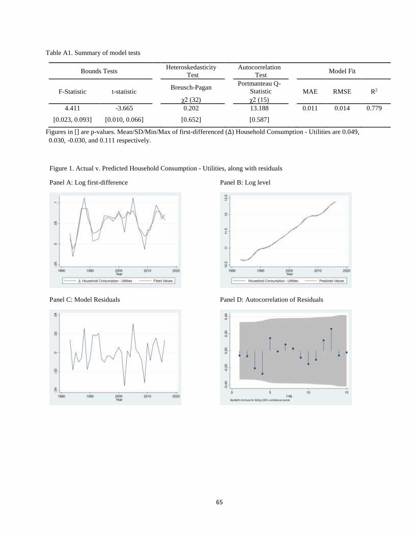
65
Table A1. Summary of model tests
Bounds Tests Heteroskedasticity
Test Autocorrelation
Test Model Fit
F-Statistic t-statistic Breusch-Pagan Portmanteau Q-
Statistic MAE RMSE R2
χ2 (32) χ2 (15)
4.411 -3.665 0.202 13.188 0.011 0.014 0.779
[0.023, 0.093] [0.010, 0.066] [0.652] [0.587]
Figures in [] are p-values. Mean/SD/Min/Max of first-differenced (∆) Household Consumption - Utilities are 0.049,
0.030, -0.030, and 0.111 respectively.
Figure 1. Actual v. Predicted Household Consumption - Utilities, along with residuals
Panel A: Log first-difference Panel B: Log level
Panel C: Model Residuals Panel D: Autocorrelation of Residuals
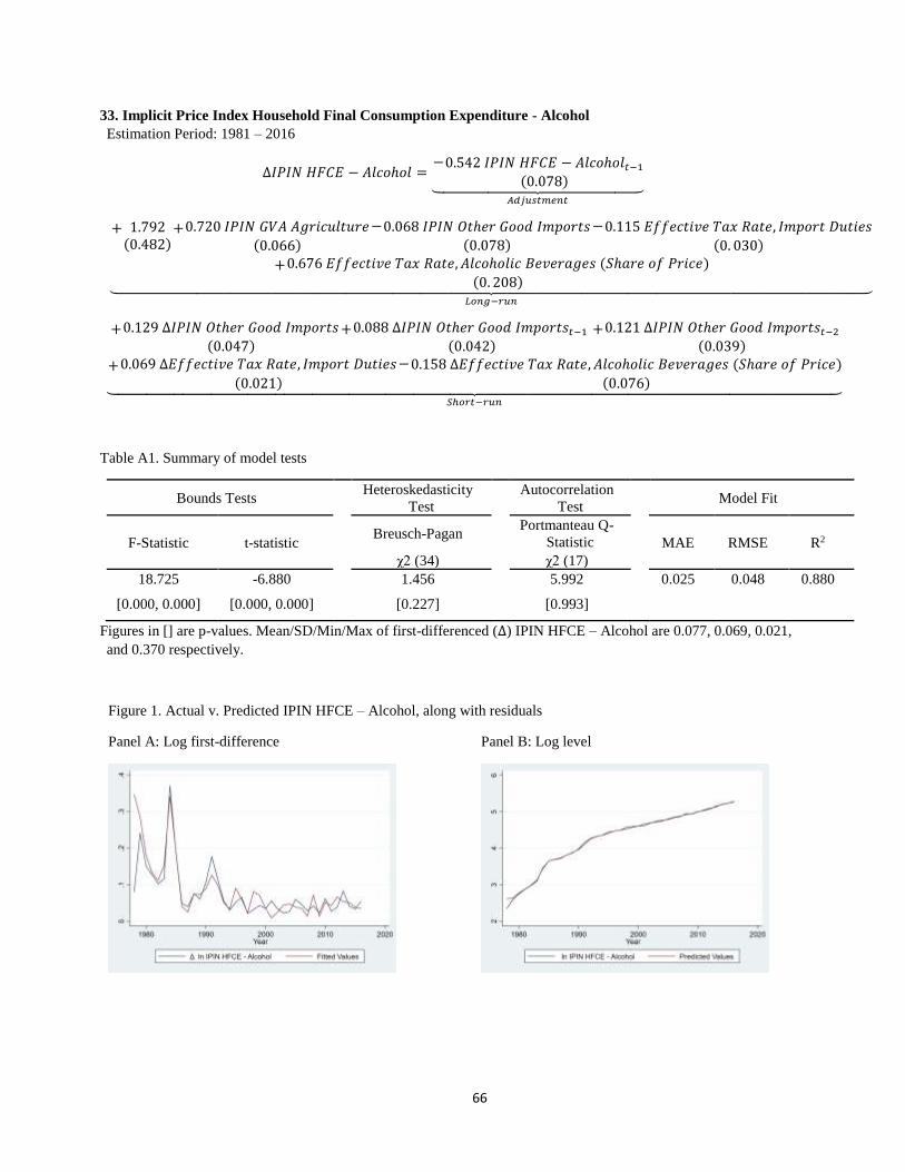
66
33. Implicit Price Index Household Final Consumption Expenditure - Alcohol
Estimation Period: 1981 – 2016
∆𝐼𝑃𝐼𝑁 𝐻𝐹𝐶𝐸 − 𝐴𝑙𝑐𝑜ℎ𝑜𝑙 =−0.542 𝐼𝑃𝐼𝑁 𝐻𝐹𝐶𝐸 − 𝐴𝑙𝑐𝑜ℎ𝑜𝑙𝑡−1
(0.078)⏟ 𝐴𝑑𝑗𝑢𝑠𝑡𝑚𝑒𝑛𝑡
+ 1.792(0.482)
+0.720 𝐼𝑃𝐼𝑁 𝐺𝑉𝐴 𝐴𝑔𝑟𝑖𝑐𝑢𝑙𝑡𝑢𝑟𝑒
(0.066)
−0.068 𝐼𝑃𝐼𝑁 𝑂𝑡ℎ𝑒𝑟 𝐺𝑜𝑜𝑑 𝐼𝑚𝑝𝑜𝑟𝑡𝑠(0.078)
−0.115 𝐸𝑓𝑓𝑒𝑐𝑡𝑖𝑣𝑒 𝑇𝑎𝑥 𝑅𝑎𝑡𝑒, 𝐼𝑚𝑝𝑜𝑟𝑡 𝐷𝑢𝑡𝑖𝑒𝑠
(0. 030)
+0.676 𝐸𝑓𝑓𝑒𝑐𝑡𝑖𝑣𝑒 𝑇𝑎𝑥 𝑅𝑎𝑡𝑒, 𝐴𝑙𝑐𝑜ℎ𝑜𝑙𝑖𝑐 𝐵𝑒𝑣𝑒𝑟𝑎𝑔𝑒𝑠 (𝑆ℎ𝑎𝑟𝑒 𝑜𝑓 𝑃𝑟𝑖𝑐𝑒)
(0. 208)⏟ 𝐿𝑜𝑛𝑔−𝑟𝑢𝑛
+0.129 ∆𝐼𝑃𝐼𝑁 𝑂𝑡ℎ𝑒𝑟 𝐺𝑜𝑜𝑑 𝐼𝑚𝑝𝑜𝑟𝑡𝑠(0.047)
+0.088 ∆𝐼𝑃𝐼𝑁 𝑂𝑡ℎ𝑒𝑟 𝐺𝑜𝑜𝑑 𝐼𝑚𝑝𝑜𝑟𝑡𝑠𝑡−1 (0.042)
+0.121 ∆𝐼𝑃𝐼𝑁 𝑂𝑡ℎ𝑒𝑟 𝐺𝑜𝑜𝑑 𝐼𝑚𝑝𝑜𝑟𝑡𝑠𝑡−2(0.039)
+0.069 ∆𝐸𝑓𝑓𝑒𝑐𝑡𝑖𝑣𝑒 𝑇𝑎𝑥 𝑅𝑎𝑡𝑒, 𝐼𝑚𝑝𝑜𝑟𝑡 𝐷𝑢𝑡𝑖𝑒𝑠
(0.021)
−0.158 ∆𝐸𝑓𝑓𝑒𝑐𝑡𝑖𝑣𝑒 𝑇𝑎𝑥 𝑅𝑎𝑡𝑒, 𝐴𝑙𝑐𝑜ℎ𝑜𝑙𝑖𝑐 𝐵𝑒𝑣𝑒𝑟𝑎𝑔𝑒𝑠 (𝑆ℎ𝑎𝑟𝑒 𝑜𝑓 𝑃𝑟𝑖𝑐𝑒)
(0.076)⏟ 𝑆ℎ𝑜𝑟𝑡−𝑟𝑢𝑛
Table A1. Summary of model tests
Bounds Tests Heteroskedasticity
Test Autocorrelation
Test Model Fit
F-Statistic t-statistic Breusch-Pagan Portmanteau Q-
Statistic MAE RMSE R2
χ2 (34) χ2 (17)
18.725 -6.880 1.456 5.992 0.025 0.048 0.880
[0.000, 0.000] [0.000, 0.000] [0.227] [0.993]
Figures in [] are p-values. Mean/SD/Min/Max of first-differenced (∆) IPIN HFCE – Alcohol are 0.077, 0.069, 0.021,
and 0.370 respectively.
Figure 1. Actual v. Predicted IPIN HFCE – Alcohol, along with residuals
Panel A: Log first-difference Panel B: Log level
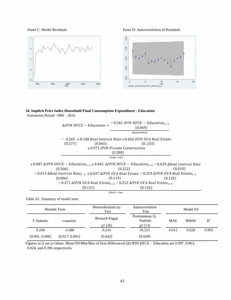
67
Panel C: Model Residuals Panel D: Autocorrelation of Residuals
34. Implicit Price Index Household Final Consumption Expenditure - Education
Estimation Period: 1989 – 2016
∆𝐼𝑃𝐼𝑁 𝐻𝐹𝐶𝐸 − 𝐸𝑑𝑢𝑐𝑎𝑡𝑖𝑜𝑛 =−0.241 𝐼𝑃𝐼𝑁 𝐻𝐹𝐶𝐸 − 𝐸𝑑𝑢𝑐𝑎𝑡𝑖𝑜𝑛𝑡−1
(0.069)⏟ 𝐴𝑑𝑗𝑢𝑠𝑡𝑚𝑒𝑛𝑡
− 0.265(0.177)
+0.140 𝑅𝑒𝑎𝑙 𝐼𝑛𝑡𝑒𝑟𝑒𝑠𝑡 𝑅𝑎𝑡𝑒(0.065)
+0.266 𝐼𝑃𝐼𝑁 𝐺𝑉𝐴 𝑅𝑒𝑎𝑙 𝐸𝑠𝑡𝑎𝑡𝑒(0. 233)
+0.971 𝐼𝑃𝐼𝑁 𝑃𝑟𝑖𝑣𝑎𝑡𝑒 𝐶𝑜𝑛𝑠𝑡𝑟𝑢𝑐𝑡𝑖𝑜𝑛(0.280)⏟
𝐿𝑜𝑛𝑔−𝑟𝑢𝑛
+0.087 ∆𝐼𝑃𝐼𝑁 𝐻𝐹𝐶𝐸 − 𝐸𝑑𝑢𝑐𝑎𝑡𝑖𝑜𝑛𝑡−1(0.206)
+0.442 ∆𝐼𝑃𝐼𝑁 𝐻𝐹𝐶𝐸 − 𝐸𝑑𝑢𝑐𝑎𝑡𝑖𝑜𝑛𝑡−2 (0.222)
−0.029 ∆𝑅𝑒𝑎𝑙 𝐼𝑛𝑡𝑒𝑟𝑒𝑠𝑡 𝑅𝑎𝑡𝑒 (0.010)
−0.013 ∆𝑅𝑒𝑎𝑙 𝐼𝑛𝑡𝑒𝑟𝑒𝑠𝑡 𝑅𝑎𝑡𝑒𝑡−1 (0.006)
+0.037 ∆𝐼𝑃𝐼𝑁 𝐺𝑉𝐴 𝑅𝑒𝑎𝑙 𝐸𝑠𝑡𝑎𝑡𝑒 (0.119)
−0.259 ∆𝐼𝑃𝐼𝑁 𝐺𝑉𝐴 𝑅𝑒𝑎𝑙 𝐸𝑠𝑡𝑎𝑡𝑒𝑡−1 (0.132)
−0.371 ∆𝐼𝑃𝐼𝑁 𝐺𝑉𝐴 𝑅𝑒𝑎𝑙 𝐸𝑠𝑡𝑎𝑡𝑒𝑡−2 (0.131)
−0.212 ∆𝐼𝑃𝐼𝑁 𝐺𝑉𝐴 𝑅𝑒𝑎𝑙 𝐸𝑠𝑡𝑎𝑡𝑒𝑡−3 (0.126)⏟
𝑆ℎ𝑜𝑟𝑡−𝑟𝑢𝑛
Table A1. Summary of model tests
Bounds Tests Heteroskedasticity
Test Autocorrelation
Test Model Fit
F-Statistic t-statistic Breusch-Pagan Portmanteau Q-
Statistic MAE RMSE R2
χ2 (26) χ2 (13)
9.249 -3.486 0.216 10.521 0.012 0.020 0.903
[0.001, 0.006] [0.017, 0.091] [0.642] [0.650]
Figures in [] are p-values. Mean/SD/Min/Max of first-differenced (∆) IPIN HFCE – Education are 0.097, 0.063,
0.024, and 0.396 respectively.

68
Figure 1. Actual v. Predicted IPIN HFCE – Education, along with residuals
Panel A: Log first-difference Panel B: Log level
Panel C: Model Residuals Panel D: Autocorrelation of Residuals
35. Implicit Price Index Household Final Consumption Expenditure – Food
Estimation Period: 1981 – 2016
∆𝐼𝑃𝐼𝑁 𝐻𝐹𝐶𝐸, 𝐹𝑜𝑜𝑑 =− 0.765 𝐼𝑃𝐼𝑁 𝐻𝐹𝐶𝐸, 𝐹𝑜𝑜𝑑𝑡−1
(0.039)⏟ 𝐴𝑑𝑗𝑢𝑠𝑡𝑚𝑒𝑛𝑡
+ 0.715(0.100)
+0.161 𝐼𝑃𝐼𝑁, 𝐴𝑔𝑟𝑖𝑐𝑢𝑙𝑡𝑢𝑟𝑎𝑙 𝐼𝑚𝑝𝑜𝑟𝑡𝑠
(0.021)+0.870 𝐼𝑃𝐼𝑁 𝐺𝑉𝐴, 𝐴𝑔𝑟𝑖𝑐𝑢𝑙𝑡𝑢𝑟𝑒
(0.019)−0.072 𝑂𝑝𝑒𝑛𝑛𝑒𝑠𝑠
(0.033)
−3.124 𝑉𝑎𝑙𝑢𝑒 𝐴𝑑𝑑𝑒𝑑 𝑇𝑎𝑥 𝑅𝑎𝑡𝑒(0.175)⏟
𝐿𝑜𝑛𝑔−𝑟𝑢𝑛
+2.997 ∆ 𝑉𝑎𝑙𝑢𝑒 𝐴𝑑𝑑𝑒𝑑 𝑇𝑎𝑥 𝑅𝑎𝑡𝑒(0.124)⏟
𝑆ℎ𝑜𝑟𝑡−𝑟𝑢𝑛
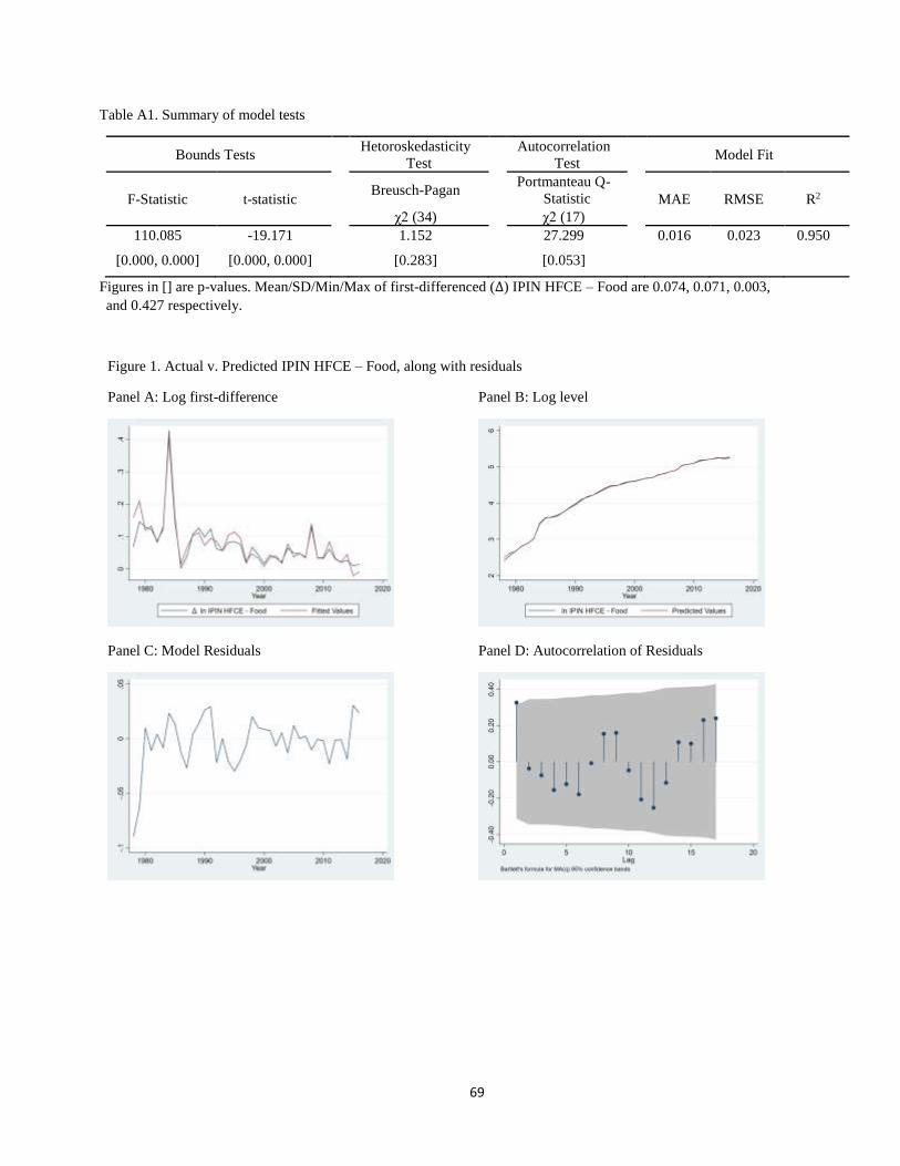
69
Table A1. Summary of model tests
Bounds Tests Hetoroskedasticity
Test Autocorrelation
Test Model Fit
F-Statistic t-statistic Breusch-Pagan Portmanteau Q-
Statistic MAE RMSE R2
χ2 (34) χ2 (17)
110.085 -19.171 1.152 27.299 0.016 0.023 0.950
[0.000, 0.000] [0.000, 0.000] [0.283] [0.053]
Figures in [] are p-values. Mean/SD/Min/Max of first-differenced (∆) IPIN HFCE – Food are 0.074, 0.071, 0.003,
and 0.427 respectively.
Figure 1. Actual v. Predicted IPIN HFCE – Food, along with residuals
Panel A: Log first-difference Panel B: Log level
Panel C: Model Residuals Panel D: Autocorrelation of Residuals
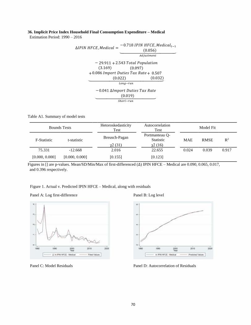
70
36. Implicit Price Index Household Final Consumption Expenditure – Medical
Estimation Period: 1990 – 2016
∆𝐼𝑃𝐼𝑁 𝐻𝐹𝐶𝐸,𝑀𝑒𝑑𝑖𝑐𝑎𝑙 =−0.718 𝐼𝑃𝐼𝑁 𝐻𝐹𝐶𝐸,𝑀𝑒𝑑𝑖𝑐𝑎𝑙𝑡−1
(0.056)⏟ 𝐴𝑑𝑗𝑢𝑠𝑡𝑚𝑒𝑛𝑡
− 29.911(3.169)
+2.543 𝑇𝑜𝑡𝑎𝑙 𝑃𝑜𝑝𝑢𝑙𝑎𝑡𝑖𝑜𝑛(0.097)
+0.086 𝐼𝑚𝑝𝑜𝑟𝑡 𝐷𝑢𝑡𝑖𝑒𝑠 𝑇𝑎𝑥 𝑅𝑎𝑡𝑒(0.022)
+ 0.507 (0.032)⏟
𝐿𝑜𝑛𝑔−𝑟𝑢𝑛
−0.041 ∆𝐼𝑚𝑝𝑜𝑟𝑡 𝐷𝑢𝑡𝑖𝑒𝑠 𝑇𝑎𝑥 𝑅𝑎𝑡𝑒(0.019)⏟
𝑆ℎ𝑜𝑟𝑡−𝑟𝑢𝑛
Table A1. Summary of model tests
Bounds Tests Hetoroskedasticity
Test Autocorrelation
Test Model Fit
F-Statistic t-statistic Breusch-Pagan Portmanteau Q-
Statistic MAE RMSE R2
χ2 (31) χ2 (16)
75.331 -12.668 2.016 22.655 0.024 0.039 0.917
[0.000, 0.000] [0.000, 0.000] [0.155] [0.123]
Figures in [] are p-values. Mean/SD/Min/Max of first-differenced (∆) IPIN HFCE – Medical are 0.090, 0.065, 0.017,
and 0.396 respectively.
Figure 1. Actual v. Predicted IPIN HFCE – Medical, along with residuals
Panel A: Log first-difference Panel B: Log level
Panel C: Model Residuals Panel D: Autocorrelation of Residuals
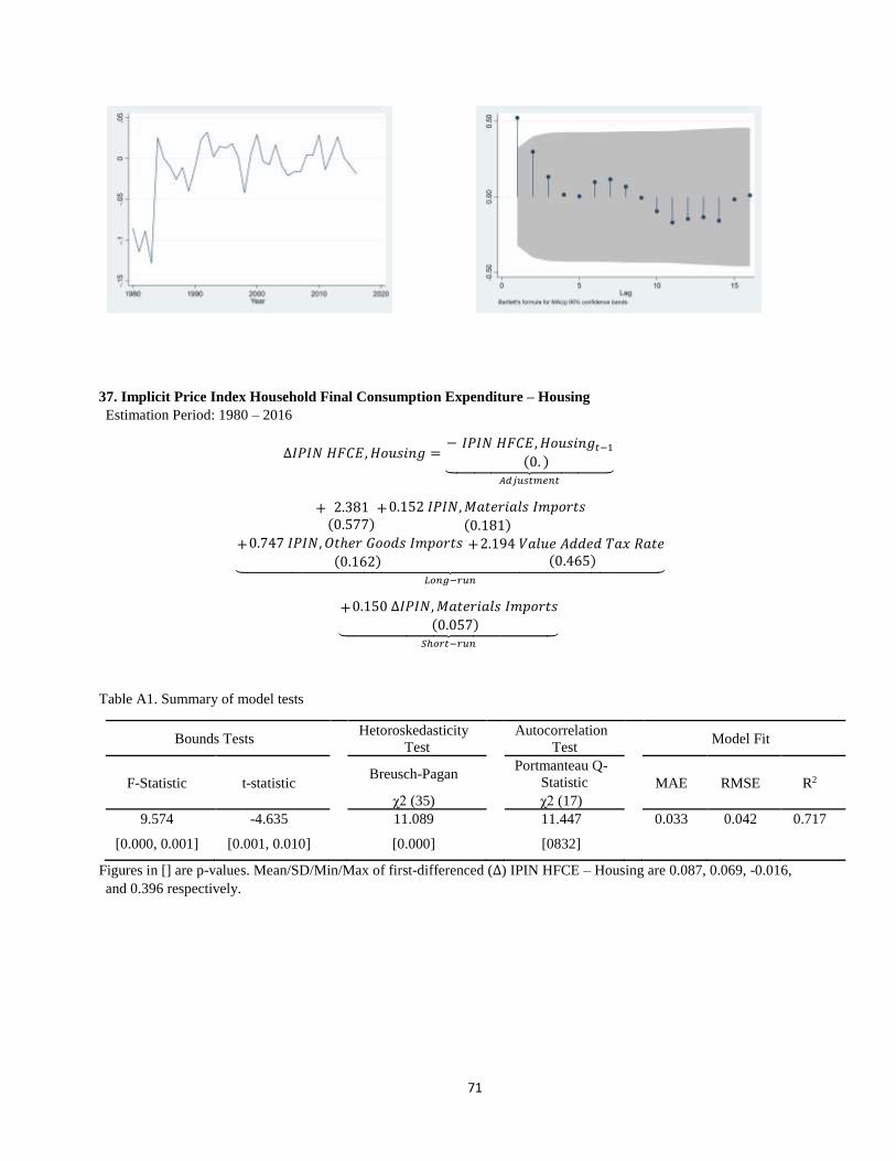
71
37. Implicit Price Index Household Final Consumption Expenditure – Housing
Estimation Period: 1980 – 2016
∆𝐼𝑃𝐼𝑁 𝐻𝐹𝐶𝐸,𝐻𝑜𝑢𝑠𝑖𝑛𝑔 =− 𝐼𝑃𝐼𝑁 𝐻𝐹𝐶𝐸,𝐻𝑜𝑢𝑠𝑖𝑛𝑔𝑡−1
(0. )⏟ 𝐴𝑑𝑗𝑢𝑠𝑡𝑚𝑒𝑛𝑡
+ 2.381(0.577)
+0.152 𝐼𝑃𝐼𝑁,𝑀𝑎𝑡𝑒𝑟𝑖𝑎𝑙𝑠 𝐼𝑚𝑝𝑜𝑟𝑡𝑠(0.181)
+0.747 𝐼𝑃𝐼𝑁, 𝑂𝑡ℎ𝑒𝑟 𝐺𝑜𝑜𝑑𝑠 𝐼𝑚𝑝𝑜𝑟𝑡𝑠 (0.162)
+2.194 𝑉𝑎𝑙𝑢𝑒 𝐴𝑑𝑑𝑒𝑑 𝑇𝑎𝑥 𝑅𝑎𝑡𝑒(0.465)⏟
𝐿𝑜𝑛𝑔−𝑟𝑢𝑛
+0.150 ∆𝐼𝑃𝐼𝑁,𝑀𝑎𝑡𝑒𝑟𝑖𝑎𝑙𝑠 𝐼𝑚𝑝𝑜𝑟𝑡𝑠(0.057)⏟
𝑆ℎ𝑜𝑟𝑡−𝑟𝑢𝑛
Table A1. Summary of model tests
Bounds Tests Hetoroskedasticity
Test Autocorrelation
Test Model Fit
F-Statistic t-statistic Breusch-Pagan Portmanteau Q-
Statistic MAE RMSE R2
χ2 (35) χ2 (17)
9.574 -4.635 11.089 11.447 0.033 0.042 0.717
[0.000, 0.001] [0.001, 0.010] [0.000] [0832]
Figures in [] are p-values. Mean/SD/Min/Max of first-differenced (∆) IPIN HFCE – Housing are 0.087, 0.069, -0.016,
and 0.396 respectively.

72
Figure 1. Actual v. Predicted IPIN HFCE – Housing, along with residuals
Panel A: Log first-difference Panel B: Log level
Panel C: Model Residuals Panel D: Autocorrelation of Residuals
38. Implicit Price Index Household Final Consumption Expenditure – Non-Alcoholic Beverages
Estimation Period: 1981 – 2016
∆𝐼𝑃𝐼𝑁 𝐻𝐹𝐶𝐸,𝑁𝑜𝑛 − 𝑎𝑙𝑐𝑜ℎ𝑜𝑙 =−0.460 𝐻𝐹𝐶𝐸,𝑁𝑜𝑛 − 𝑎𝑙𝑐𝑜ℎ𝑜𝑙𝑡−1
(0.098)⏟ 𝐴𝑑𝑗𝑢𝑠𝑡𝑚𝑒𝑛𝑡
+ 0.356(0.091)
+0.106 𝐼𝑃𝐼𝑁, 𝐴𝑔𝑟𝑖𝑐𝑢𝑙𝑡𝑢𝑟𝑎𝑙 𝐼𝑚𝑝𝑜𝑟𝑡𝑠
(0.034)+0.839 𝐼𝑃𝐼𝑁 𝐺𝑉𝐴, 𝐴𝑔𝑟𝑖𝑐𝑢𝑙𝑡𝑢𝑟𝑒
(0.043)⏟ 𝐿𝑜𝑛𝑔−𝑟𝑢𝑛
+0.239 ∆𝐻𝐹𝐶𝐸,𝑁𝑜𝑛 − 𝑎𝑙𝑐𝑜ℎ𝑜𝑙𝑡−1(0.066)
+0.218 ∆𝐼𝑃𝐼𝑁 𝐺𝑉𝐴, 𝐴𝑔𝑟𝑖𝑐𝑢𝑙𝑡𝑢𝑟𝑒
(0.096)⏟ 𝑆ℎ𝑜𝑟𝑡−𝑟𝑢𝑛
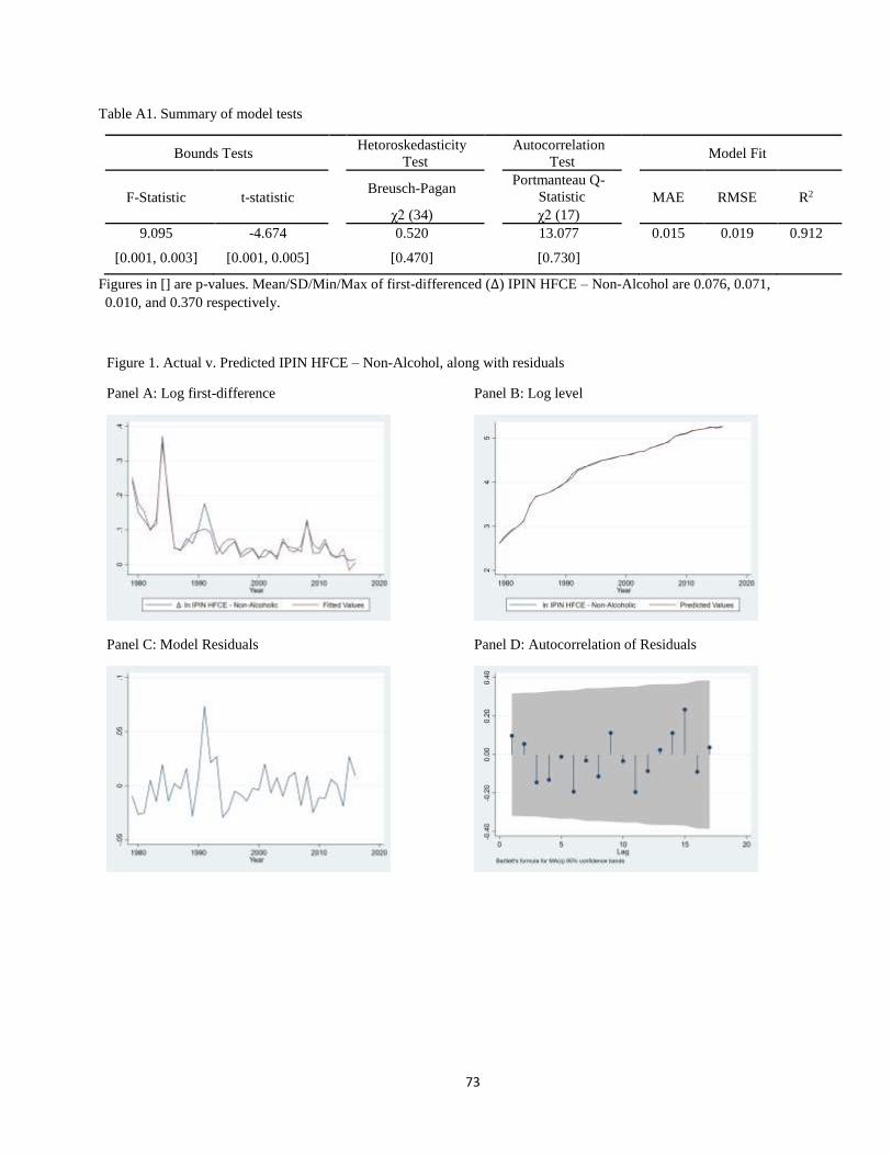
73
Table A1. Summary of model tests
Bounds Tests Hetoroskedasticity
Test Autocorrelation
Test Model Fit
F-Statistic t-statistic Breusch-Pagan Portmanteau Q-
Statistic MAE RMSE R2
χ2 (34) χ2 (17)
9.095 -4.674 0.520 13.077 0.015 0.019 0.912
[0.001, 0.003] [0.001, 0.005] [0.470] [0.730]
Figures in [] are p-values. Mean/SD/Min/Max of first-differenced (∆) IPIN HFCE – Non-Alcohol are 0.076, 0.071,
0.010, and 0.370 respectively.
Figure 1. Actual v. Predicted IPIN HFCE – Non-Alcohol, along with residuals
Panel A: Log first-difference Panel B: Log level
Panel C: Model Residuals Panel D: Autocorrelation of Residuals

74
39. Implicit Price Index Household Final Consumption Expenditure – Miscellaneous
Estimation Period: 1990 – 2016
∆𝐼𝑃𝐼𝑁 𝐻𝐹𝐶𝐸,𝑀𝑖𝑠𝑐𝑒𝑙𝑙𝑎𝑛𝑒𝑜𝑢𝑠 =− 0.352 𝐼𝑃𝐼𝑁 𝐻𝐹𝐶𝐸,𝑀𝑖𝑠𝑐𝑒𝑙𝑙𝑎𝑛𝑒𝑜𝑢𝑠𝑡−1
(0.097)⏟ 𝐴𝑑𝑗𝑢𝑠𝑡𝑚𝑒𝑛𝑡
− 0.422(0.221)
+0.134 𝑅𝑒𝑣𝑒𝑟𝑠𝑒 𝑅𝑒𝑝𝑢𝑟𝑐ℎ𝑎𝑠𝑒 𝑅𝑎𝑡𝑒(0.081)
−2.095 𝐼𝑃𝐼𝑁 𝐻𝐹𝐶𝐸, 𝐸𝑑𝑢𝑐𝑎𝑡𝑖𝑜𝑛(0.565)
+3.300 𝐼𝑃𝐼𝑁 𝐻𝐹𝐶𝐸,𝑀𝑒𝑑𝑖𝑐𝑎𝑙(0.603)⏟
𝐿𝑜𝑛𝑔−𝑟𝑢𝑛
Table A1. Summary of model tests
Bounds Tests Hetoroskedasticity
Test Autocorrelation
Test Model Fit
F-Statistic t-statistic Breusch-Pagan Portmanteau Q-
Statistic MAE RMSE R2
χ2 (25) χ2 (13)
19.981 -3.607 1.021 8.751 0.018 0.022 0.784
[0.000, 0.000] [0.013, 0.081] [0.312] [0.791]
Figures in [] are p-values. Mean/SD/Min/Max of first-differenced (∆) IPIN HFCE – Miscellaneous are 0.084, 0.079, -
0.009, and 0.464 respectively.
Figure 1. Actual v. Predicted IPIN HFCE – Miscellaneous, along with residuals
Panel A: Log first-difference Panel B: Log level

75
Panel C: Model Residuals Panel D: Autocorrelation of Residuals
40. Implicit Price Index Household Final Consumption Expenditure – Tobacco
Estimation Period: 1982 – 2016
∆𝐼𝑃𝐼𝑁 𝐻𝐹𝐶𝐸, 𝑇𝑜𝑏𝑎𝑐𝑐𝑜 =− 1.514 𝐼𝑃𝐼𝑁 𝐻𝐹𝐶𝐸, 𝑇𝑜𝑏𝑎𝑐𝑐𝑜𝑡−1
(0.168)⏟ 𝐴𝑑𝑗𝑢𝑠𝑡𝑚𝑒𝑛𝑡
+ 0.056(0.203)
+0.120 𝑇𝑜𝑏𝑎𝑐𝑐𝑜 𝑇𝑎𝑥 𝑅𝑎𝑡𝑒 (𝑆ℎ𝑎𝑟𝑒 𝑜𝑓 𝑃𝑟𝑖𝑐𝑒)
(0.009)+0.705 𝐼𝑃𝐼𝑁 𝐺𝑉𝐴, 𝐴𝑔𝑟𝑖𝑐𝑢𝑙𝑡𝑢𝑟𝑒
(0.014)
+0.087 𝐼𝑃𝐼𝑁, 𝐴𝑔𝑟𝑖𝑐𝑢𝑙𝑡𝑢𝑟𝑎𝑙 𝐼𝑚𝑝𝑜𝑟𝑡𝑠
(0.014)+0.149 𝑊𝑎𝑔𝑒 𝐼𝑛𝑑𝑒𝑥,𝑀𝑎𝑛𝑢𝑓𝑎𝑐𝑡𝑢𝑟𝑖𝑛𝑔
(0.023)+0.247 𝑈𝑆𝐷 𝑁𝑜𝑚𝑖𝑛𝑎𝑙 𝐸𝑥𝑐ℎ𝑎𝑛𝑔𝑒 𝑅𝑎𝑡𝑒
(0.015)⏟ 𝐿𝑜𝑛𝑔−𝑟𝑢𝑛
−0.524 ∆𝐼𝑃𝐼𝑁 𝐺𝑉𝐴, 𝐴𝑔𝑟𝑖𝑐𝑢𝑙𝑡𝑢𝑟𝑒
(0.128)
−0.155 ∆𝑈𝑆𝐷 𝑁𝑜𝑚𝑖𝑛𝑎𝑙 𝐸𝑥𝑐ℎ𝑎𝑛𝑔𝑒 𝑅𝑎𝑡𝑒
(0.061)⏟ 𝑆ℎ𝑜𝑟𝑡−𝑟𝑢𝑛
Table A1. Summary of model tests
Bounds Tests Hetoroskedasticity
Test Autocorrelation
Test Model Fit
F-Statistic t-statistic Breusch-Pagan Portmanteau Q-
Statistic MAE RMSE R2
χ2 (33) χ2 (17)
16.292 -9.006 0.229 14.426 0.027 0.051 0.939
[0.000, 0.000] [0.000, 0.000] [0.631] [0.636]
Figures in [] are p-values. Mean/SD/Min/Max of first-differenced (∆) IPIN HFCE – Tobacco are 0.076, 0.075, 0.022,
and 0.464 respectively.
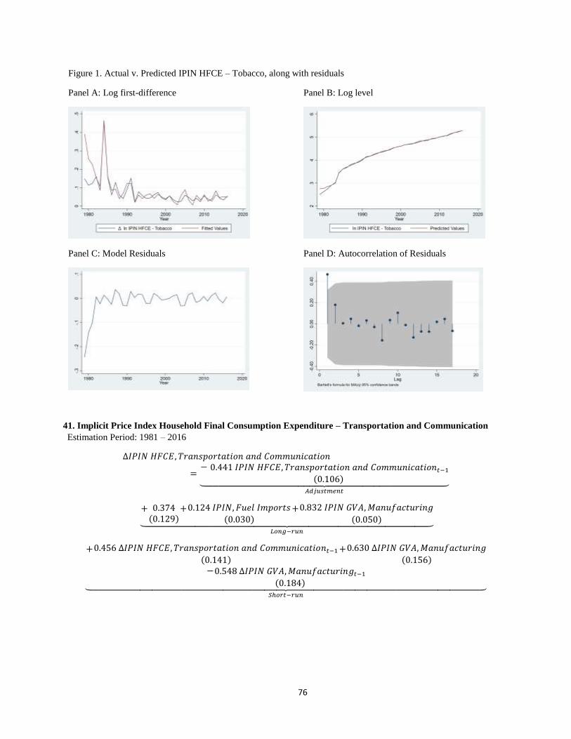
76
Figure 1. Actual v. Predicted IPIN HFCE – Tobacco, along with residuals
Panel A: Log first-difference Panel B: Log level
Panel C: Model Residuals Panel D: Autocorrelation of Residuals
41. Implicit Price Index Household Final Consumption Expenditure – Transportation and Communication
Estimation Period: 1981 – 2016
∆𝐼𝑃𝐼𝑁 𝐻𝐹𝐶𝐸, 𝑇𝑟𝑎𝑛𝑠𝑝𝑜𝑟𝑡𝑎𝑡𝑖𝑜𝑛 𝑎𝑛𝑑 𝐶𝑜𝑚𝑚𝑢𝑛𝑖𝑐𝑎𝑡𝑖𝑜𝑛
=− 0.441 𝐼𝑃𝐼𝑁 𝐻𝐹𝐶𝐸, 𝑇𝑟𝑎𝑛𝑠𝑝𝑜𝑟𝑡𝑎𝑡𝑖𝑜𝑛 𝑎𝑛𝑑 𝐶𝑜𝑚𝑚𝑢𝑛𝑖𝑐𝑎𝑡𝑖𝑜𝑛𝑡−1
(0.106)⏟ 𝐴𝑑𝑗𝑢𝑠𝑡𝑚𝑒𝑛𝑡
+ 0.374(0.129)
+0.124 𝐼𝑃𝐼𝑁, 𝐹𝑢𝑒𝑙 𝐼𝑚𝑝𝑜𝑟𝑡𝑠(0.030)
+0.832 𝐼𝑃𝐼𝑁 𝐺𝑉𝐴,𝑀𝑎𝑛𝑢𝑓𝑎𝑐𝑡𝑢𝑟𝑖𝑛𝑔
(0.050)⏟ 𝐿𝑜𝑛𝑔−𝑟𝑢𝑛
+0.456 ∆𝐼𝑃𝐼𝑁 𝐻𝐹𝐶𝐸, 𝑇𝑟𝑎𝑛𝑠𝑝𝑜𝑟𝑡𝑎𝑡𝑖𝑜𝑛 𝑎𝑛𝑑 𝐶𝑜𝑚𝑚𝑢𝑛𝑖𝑐𝑎𝑡𝑖𝑜𝑛𝑡−1(0.141)
+0.630 ∆𝐼𝑃𝐼𝑁 𝐺𝑉𝐴,𝑀𝑎𝑛𝑢𝑓𝑎𝑐𝑡𝑢𝑟𝑖𝑛𝑔
(0.156)−0.548 ∆𝐼𝑃𝐼𝑁 𝐺𝑉𝐴,𝑀𝑎𝑛𝑢𝑓𝑎𝑐𝑡𝑢𝑟𝑖𝑛𝑔𝑡−1
(0.184)⏟ 𝑆ℎ𝑜𝑟𝑡−𝑟𝑢𝑛
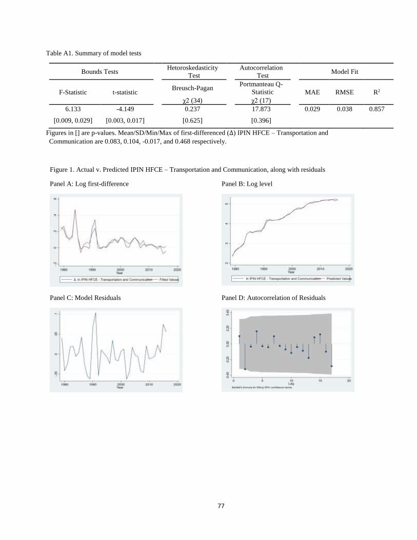
77
Table A1. Summary of model tests
Bounds Tests Hetoroskedasticity
Test Autocorrelation
Test Model Fit
F-Statistic t-statistic Breusch-Pagan Portmanteau Q-
Statistic MAE RMSE R2
χ2 (34) χ2 (17)
6.133 -4.149 0.237 17.873 0.029 0.038 0.857
[0.009, 0.029] [0.003, 0.017] [0.625] [0.396]
Figures in [] are p-values. Mean/SD/Min/Max of first-differenced (∆) IPIN HFCE – Transportation and
Communication are 0.083, 0.104, -0.017, and 0.468 respectively.
Figure 1. Actual v. Predicted IPIN HFCE – Transportation and Communication, along with residuals
Panel A: Log first-difference Panel B: Log level
Panel C: Model Residuals Panel D: Autocorrelation of Residuals

78
42. Implicit Price Index Household Final Consumption Expenditure – Utilities
Estimation Period: 1981 – 2016
∆𝐼𝑃𝐼𝑁 𝐻𝐹𝐶𝐸, 𝑈𝑡𝑖𝑙𝑖𝑡𝑖𝑒𝑠 =−0.881 𝐼𝑃𝐼𝑁 𝐻𝐹𝐶𝐸, 𝑈𝑡𝑖𝑙𝑖𝑡𝑖𝑒𝑠𝑡−1
(0.139)⏟ 𝐴𝑑𝑗𝑢𝑠𝑡𝑚𝑒𝑛𝑡
+ 0.750(0.284)
+0.656 𝐼𝑃𝐼𝑁 𝐺𝑉𝐴,𝑊𝑎𝑡𝑒𝑟(0.072)
+0.100 𝐼𝑃𝐼𝑁 𝐺𝑉𝐴, 𝐸𝑙𝑒𝑐𝑡𝑟𝑖𝑐𝑖𝑡𝑦 𝑎𝑛𝑑 𝑆𝑡𝑒𝑎𝑚
(0.120)
+0.099 𝑈𝑆𝐷 𝑁𝑜𝑚𝑖𝑛𝑎𝑙 𝐸𝑥𝑐ℎ𝑎𝑛𝑔𝑒 𝑅𝑎𝑡𝑒
(0.097)+0.186 𝐽𝑃𝑌 𝑁𝑜𝑚𝑖𝑛𝑎𝑙 𝐸𝑥𝑐ℎ𝑎𝑛𝑔𝑒 𝑅𝑎𝑡𝑒
(0.050)⏟ 𝐿𝑜𝑛𝑔−𝑟𝑢𝑛
+0.249 ∆𝐼𝑃𝐼𝑁 𝐻𝐹𝐶𝐸, 𝑈𝑡𝑖𝑙𝑖𝑡𝑖𝑒𝑠𝑡−1(0.127)
−0.379 ∆𝐼𝑃𝐼𝑁 𝐻𝐹𝐶𝐸, 𝑈𝑡𝑖𝑙𝑖𝑡𝑖𝑒𝑠𝑡−2(0.126)
−0.266 ∆𝐼𝑃𝐼𝑁 𝐺𝑉𝐴,𝑊𝑎𝑡𝑒𝑟(0.103)
−0.345 ∆𝐼𝑃𝐼𝑁 𝐺𝑉𝐴,𝑊𝑎𝑡𝑒𝑟𝑡−1(0.082)
+0.022 ∆𝐼𝑃𝐼𝑁 𝐺𝑉𝐴,𝑊𝑎𝑡𝑒𝑟𝑡−2(0.068)
−0.130 ∆𝐼𝑃𝐼𝑁 𝐺𝑉𝐴,𝑊𝑎𝑡𝑒𝑟𝑡−3(0.060)
−0.012 ∆𝐼𝑃𝐼𝑁 𝐺𝑉𝐴, 𝐸𝑙𝑒𝑐𝑡𝑟𝑖𝑐𝑖𝑡𝑦 𝑎𝑛𝑑 𝑆𝑡𝑒𝑎𝑚
(0.112)+0.319∆𝐼𝑃𝐼𝑁 𝐺𝑉𝐴, 𝐸𝑙𝑒𝑐𝑡𝑟𝑖𝑐𝑖𝑡𝑦 𝑎𝑛𝑑 𝑆𝑡𝑒𝑎𝑚𝑡−1
(0.097)
+0.418 ∆𝐼𝑃𝐼𝑁 𝐺𝑉𝐴, 𝐸𝑙𝑒𝑐𝑡𝑟𝑖𝑐𝑖𝑡𝑦 𝑎𝑛𝑑 𝑆𝑡𝑒𝑎𝑚𝑡−2
(0.084)+0.172 ∆𝐼𝑃𝐼𝑁 𝐺𝑉𝐴, 𝐸𝑙𝑒𝑐𝑡𝑟𝑖𝑐𝑖𝑡𝑦 𝑎𝑛𝑑 𝑆𝑡𝑒𝑎𝑚𝑡−3
(0.079)
+0.334 ∆𝑈𝑆𝐷 𝑁𝑜𝑚𝑖𝑛𝑎𝑙 𝐸𝑥𝑐ℎ𝑎𝑛𝑔𝑒 𝑅𝑎𝑡𝑒
(0.116)
−0.101 ∆𝐽𝑃𝑌 𝑁𝑜𝑚𝑖𝑛𝑎𝑙 𝐸𝑥𝑐ℎ𝑎𝑛𝑔𝑒 𝑅𝑎𝑡𝑒
(0.072)⏟ 𝑆ℎ𝑜𝑟𝑡−𝑟𝑢𝑛
Table A1. Summary of model tests
Bounds Tests Hetoroskedasticity
Test Autocorrelation
Test Model Fit
F-Statistic t-statistic Breusch-Pagan Portmanteau Q-
Statistic MAE RMSE R2
χ2 (34) χ2 (16)
11.653 -6.296 0.219 6.928 0.016 0.023 0.950
[0.000, 0.001] [0.000, 0.001] [0.639] [0.974]
Figures in [] are p-values. Mean/SD/Min/Max of first-differenced (∆) IPIN HFCE – Utilities are 0.091, 0.094, -0.018,
and 0.441 respectively.
Figure 1. Actual v. Predicted IPIN HFCE – Utilities, along with residuals
Panel A: Log first-difference Panel B: Log level
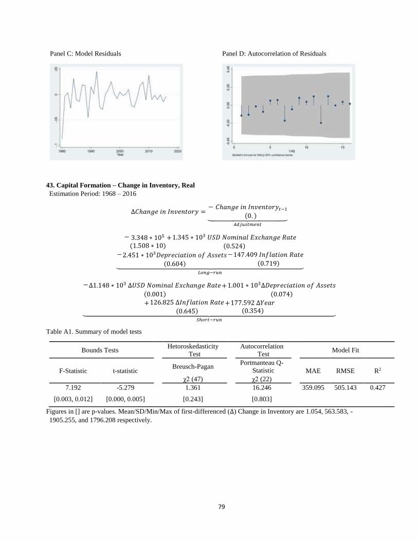
79
Panel C: Model Residuals Panel D: Autocorrelation of Residuals
43. Capital Formation – Change in Inventory, Real
Estimation Period: 1968 – 2016
∆𝐶ℎ𝑎𝑛𝑔𝑒 𝑖𝑛 𝐼𝑛𝑣𝑒𝑛𝑡𝑜𝑟𝑦 =− 𝐶ℎ𝑎𝑛𝑔𝑒 𝑖𝑛 𝐼𝑛𝑣𝑒𝑛𝑡𝑜𝑟𝑦𝑡−1
(0. )⏟ 𝐴𝑑𝑗𝑢𝑠𝑡𝑚𝑒𝑛𝑡
− 3.348 ∗ 105
(1.508 ∗ 10)+1.345 ∗ 103 𝑈𝑆𝐷 𝑁𝑜𝑚𝑖𝑛𝑎𝑙 𝐸𝑥𝑐ℎ𝑎𝑛𝑔𝑒 𝑅𝑎𝑡𝑒
(0.524)
−2.451 ∗ 103𝐷𝑒𝑝𝑟𝑒𝑐𝑖𝑎𝑡𝑖𝑜𝑛 𝑜𝑓 𝐴𝑠𝑠𝑒𝑡𝑠
(0.604)
−147.409 𝐼𝑛𝑓𝑙𝑎𝑡𝑖𝑜𝑛 𝑅𝑎𝑡𝑒
(0.719)⏟ 𝐿𝑜𝑛𝑔−𝑟𝑢𝑛
−∆1.148 ∗ 103 ∆𝑈𝑆𝐷 𝑁𝑜𝑚𝑖𝑛𝑎𝑙 𝐸𝑥𝑐ℎ𝑎𝑛𝑔𝑒 𝑅𝑎𝑡𝑒
(0.001)+1.001 ∗ 103∆𝐷𝑒𝑝𝑟𝑒𝑐𝑖𝑎𝑡𝑖𝑜𝑛 𝑜𝑓 𝐴𝑠𝑠𝑒𝑡𝑠
(0.074)
+126.825 ∆𝐼𝑛𝑓𝑙𝑎𝑡𝑖𝑜𝑛 𝑅𝑎𝑡𝑒
(0.645)+177.592 ∆𝑌𝑒𝑎𝑟
(0.354)⏟ 𝑆ℎ𝑜𝑟𝑡−𝑟𝑢𝑛
Table A1. Summary of model tests
Bounds Tests Hetoroskedasticity
Test Autocorrelation
Test Model Fit
F-Statistic t-statistic Breusch-Pagan Portmanteau Q-
Statistic MAE RMSE R2
χ2 (47) χ2 (22)
7.192 -5.279 1.361 16.246 359.095 505.143 0.427
[0.003, 0.012] [0.000, 0.005] [0.243] [0.803]
Figures in [] are p-values. Mean/SD/Min/Max of first-differenced (∆) Change in Inventory are 1.054, 563.583, -
1905.255, and 1796.208 respectively.

80
Figure 1. Actual v. Predicted Change in Inventory, along with residuals
Panel A: Log first-difference Panel B: Log level
Panel C: Model Residuals Panel D: Autocorrelation of Residuals
44. Capital Formation – Fixed – Durables, Real
Estimation Period: 1990 – 2016
∆𝐷𝑢𝑟𝑎𝑏𝑙𝑒𝑠 =−0.855 𝐷𝑢𝑟𝑎𝑏𝑙𝑒𝑠𝑡−1
(0.160)⏟ 𝐴𝑑𝑗𝑢𝑠𝑡𝑚𝑒𝑛𝑡
− 2.555(1.734)
+0.700 𝑀𝑎𝑐ℎ𝑖𝑛𝑒𝑟𝑦 𝐼𝑚𝑝𝑜𝑟𝑡𝑠, 𝑅𝑒𝑎𝑙
(0.096)−0.477 𝑅𝑒𝑣𝑒𝑟𝑠𝑒 𝑅𝑒𝑝𝑢𝑟𝑐ℎ𝑎𝑠𝑒 𝑅𝑎𝑡𝑒
(0.033)+0.917 𝑈𝑆𝐷 𝑅𝑒𝑎𝑙 𝐸𝑥𝑐ℎ𝑎𝑛𝑔𝑒 𝑅𝑎𝑡𝑒
(0.244)⏟ 𝐿𝑜𝑛𝑔−𝑟𝑢𝑛
+0.699 ∆𝐷𝑢𝑟𝑎𝑏𝑙𝑒𝑠(0.188)
+0.118 ∆𝑀𝑎𝑐ℎ𝑖𝑛𝑒𝑟𝑦 𝐼𝑚𝑝𝑜𝑟𝑡𝑠, 𝑅𝑒𝑎𝑙
(0.121)
−0.385 ∆𝑀𝑎𝑐ℎ𝑖𝑛𝑒𝑟𝑦 𝐼𝑚𝑝𝑜𝑟𝑡𝑠, 𝑅𝑒𝑎𝑙
(0.101)
+0.180 ∆𝑅𝑒𝑣𝑒𝑟𝑠𝑒 𝑅𝑒𝑝𝑢𝑟𝑐ℎ𝑎𝑠𝑒 𝑅𝑎𝑡𝑒(0.095)
−1.127 ∆𝑈𝑆𝐷 𝑅𝑒𝑎𝑙 𝐸𝑥𝑐ℎ𝑎𝑛𝑔𝑒 𝑅𝑎𝑡𝑒
(0.309)
−0.593 ∆𝑈𝑆𝐷 𝑅𝑒𝑎𝑙 𝐸𝑥𝑐ℎ𝑎𝑛𝑔𝑒 𝑅𝑎𝑡𝑒
(0.227)⏟ 𝑆ℎ𝑜𝑟𝑡−𝑟𝑢𝑛
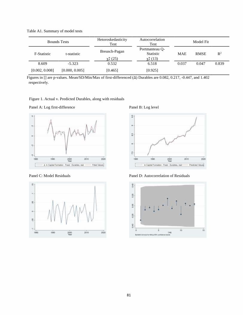
81
Table A1. Summary of model tests
Bounds Tests Hetoroskedasticity
Test Autocorrelation
Test Model Fit
F-Statistic t-statistic Breusch-Pagan Portmanteau Q-
Statistic MAE RMSE R2
χ2 (25) χ2 (13)
8.609 -5.323 0.532 6.518 0.037 0.047 0.839
[0.002, 0.008] [0.000, 0.005] [0.465] [0.925]
Figures in [] are p-values. Mean/SD/Min/Max of first-differenced (∆) Durables are 0.082, 0.217, -0.447, and 1.402
respectively.
Figure 1. Actual v. Predicted Durables, along with residuals
Panel A: Log first-difference Panel B: Log level
Panel C: Model Residuals Panel D: Autocorrelation of Residuals

82
45. Capital Formation - Fixed - Private Construction, Real
Estimation Period: 1977 – 2016
∆𝑃𝑟𝑖𝑣𝑎𝑡𝑒 𝐶𝑜𝑛𝑠𝑡𝑟𝑢𝑐𝑡𝑖𝑜𝑛 =−0.381 𝑃𝑟𝑖𝑣𝑎𝑡𝑒 𝐶𝑜𝑛𝑠𝑡𝑟𝑢𝑐𝑡𝑖𝑜𝑛𝑡−1
(0.066)⏟ 𝐴𝑑𝑗𝑢𝑠𝑡𝑚𝑒𝑛𝑡
+ 13.557(4.388)
+0.778 𝐷𝑢𝑟𝑎𝑏𝑙𝑒𝑠(0.150)
−0.631 𝐿𝑒𝑛𝑑𝑖𝑛𝑔 𝑅𝑎𝑡𝑒
(0.143)⏟ 𝐿𝑜𝑛𝑔−𝑟𝑢𝑛
−0.006 ∆𝑌𝑒𝑎𝑟(0. )⏟
𝑆ℎ𝑜𝑟𝑡−𝑟𝑢𝑛
Table A1. Summary of model tests
Bounds Tests Hetoroskedasticity
Test Autocorrelation
Test Model Fit
F-Statistic t-statistic Breusch-Pagan Portmanteau Q-
Statistic MAE RMSE R2
χ2 (38) χ2 (20)
21.066 -5.765 2.348 9.007 0.064 0.088 0.662
[0.000, 0.000] [0.000, 0.001] [0.125] [0.982]
Figures in [] are p-values. Mean/SD/Min/Max of first-differenced (∆) Private Construction are 0.040, 0.151, -0.491,
and 0.435 respectively.
Figure 1. Actual v. Predicted Private Construction, along with residuals
Panel A: Log first-difference Panel B: Log level
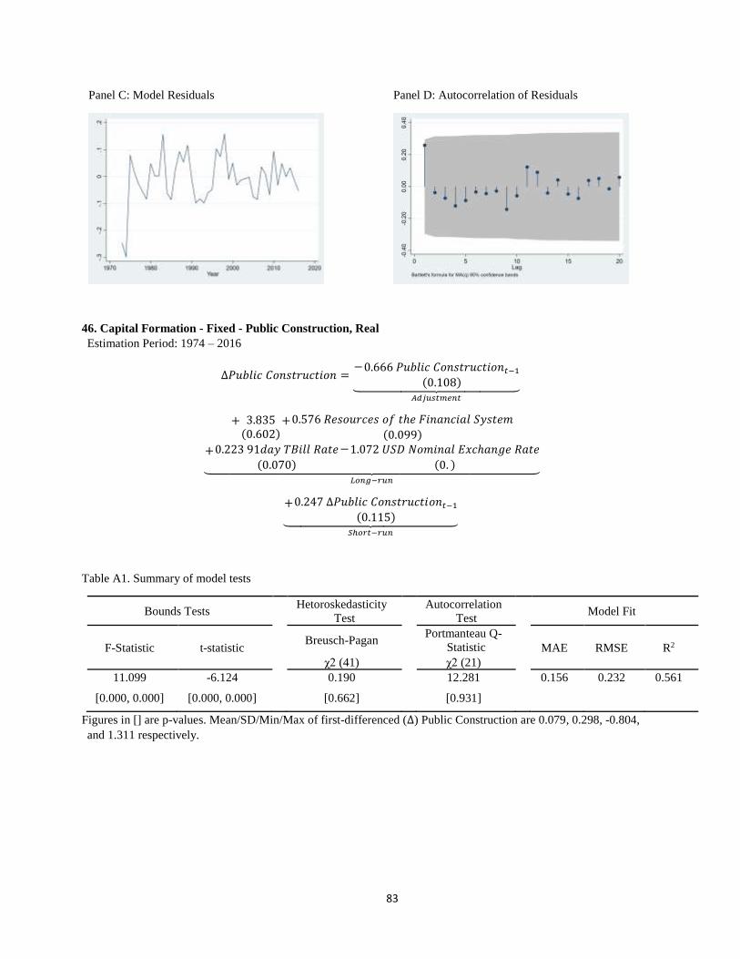
83
Panel C: Model Residuals Panel D: Autocorrelation of Residuals
46. Capital Formation - Fixed - Public Construction, Real
Estimation Period: 1974 – 2016
∆𝑃𝑢𝑏𝑙𝑖𝑐 𝐶𝑜𝑛𝑠𝑡𝑟𝑢𝑐𝑡𝑖𝑜𝑛 =−0.666 𝑃𝑢𝑏𝑙𝑖𝑐 𝐶𝑜𝑛𝑠𝑡𝑟𝑢𝑐𝑡𝑖𝑜𝑛𝑡−1
(0.108)⏟ 𝐴𝑑𝑗𝑢𝑠𝑡𝑚𝑒𝑛𝑡
+ 3.835(0.602)
+0.576 𝑅𝑒𝑠𝑜𝑢𝑟𝑐𝑒𝑠 𝑜𝑓 𝑡ℎ𝑒 𝐹𝑖𝑛𝑎𝑛𝑐𝑖𝑎𝑙 𝑆𝑦𝑠𝑡𝑒𝑚
(0.099)
+0.223 91𝑑𝑎𝑦 𝑇𝐵𝑖𝑙𝑙 𝑅𝑎𝑡𝑒
(0.070)
−1.072 𝑈𝑆𝐷 𝑁𝑜𝑚𝑖𝑛𝑎𝑙 𝐸𝑥𝑐ℎ𝑎𝑛𝑔𝑒 𝑅𝑎𝑡𝑒
(0. )⏟ 𝐿𝑜𝑛𝑔−𝑟𝑢𝑛
+0.247 ∆𝑃𝑢𝑏𝑙𝑖𝑐 𝐶𝑜𝑛𝑠𝑡𝑟𝑢𝑐𝑡𝑖𝑜𝑛𝑡−1(0.115)⏟
𝑆ℎ𝑜𝑟𝑡−𝑟𝑢𝑛
Table A1. Summary of model tests
Bounds Tests Hetoroskedasticity
Test Autocorrelation
Test Model Fit
F-Statistic t-statistic Breusch-Pagan Portmanteau Q-
Statistic MAE RMSE R2
χ2 (41) χ2 (21)
11.099 -6.124 0.190 12.281 0.156 0.232 0.561
[0.000, 0.000] [0.000, 0.000] [0.662] [0.931]
Figures in [] are p-values. Mean/SD/Min/Max of first-differenced (∆) Public Construction are 0.079, 0.298, -0.804,
and 1.311 respectively.
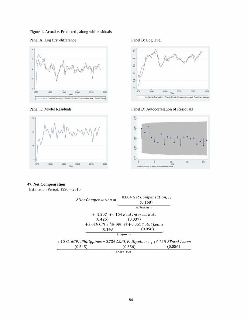
84
Figure 1. Actual v. Predicted , along with residuals
Panel A: Log first-difference Panel B: Log level
Panel C: Model Residuals Panel D: Autocorrelation of Residuals
47. Net Compensation
Estimation Period: 1996 – 2016
∆𝑁𝑒𝑡 𝐶𝑜𝑚𝑝𝑒𝑛𝑠𝑎𝑡𝑖𝑜𝑛 =− 0.604 𝑁𝑒𝑡 𝐶𝑜𝑚𝑝𝑒𝑛𝑠𝑎𝑡𝑖𝑜𝑛𝑡−1
(0.168)⏟ 𝐴𝑑𝑗𝑢𝑠𝑡𝑚𝑒𝑛𝑡
+ 1.207(0.425)
+0.104 𝑅𝑒𝑎𝑙 𝐼𝑛𝑡𝑒𝑟𝑒𝑠𝑡 𝑅𝑎𝑡𝑒(0.037)
+2.616 𝐶𝑃𝐼, 𝑃ℎ𝑖𝑙𝑖𝑝𝑝𝑖𝑛𝑒𝑠
(0.143)+0.051 𝑇𝑜𝑡𝑎𝑙 𝐿𝑜𝑎𝑛𝑠
(0.058)⏟ 𝐿𝑜𝑛𝑔−𝑟𝑢𝑛
+1.381 ∆𝐶𝑃𝐼, 𝑃ℎ𝑖𝑙𝑖𝑝𝑝𝑖𝑛𝑒𝑠(0.545)
−0.736 ∆𝐶𝑃𝐼, 𝑃ℎ𝑖𝑙𝑖𝑝𝑝𝑖𝑛𝑒𝑠𝑡−1(0.356)
+0.219 ∆𝑇𝑜𝑡𝑎𝑙 𝐿𝑜𝑎𝑛𝑠(0.056)⏟
𝑆ℎ𝑜𝑟𝑡−𝑟𝑢𝑛
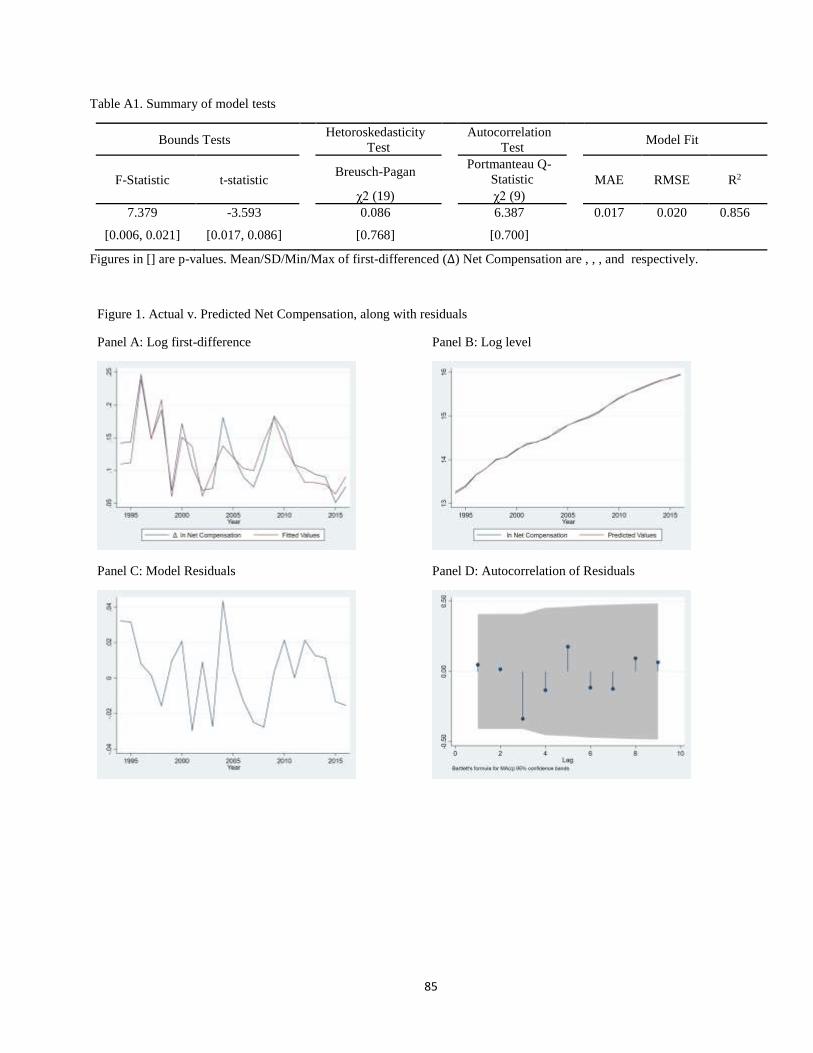
85
Table A1. Summary of model tests
Bounds Tests Hetoroskedasticity
Test Autocorrelation
Test Model Fit
F-Statistic t-statistic Breusch-Pagan Portmanteau Q-
Statistic MAE RMSE R2
χ2 (19) χ2 (9)
7.379 -3.593 0.086 6.387 0.017 0.020 0.856
[0.006, 0.021] [0.017, 0.086] [0.768] [0.700]
Figures in [] are p-values. Mean/SD/Min/Max of first-differenced (∆) Net Compensation are , , , and respectively.
Figure 1. Actual v. Predicted Net Compensation, along with residuals
Panel A: Log first-difference Panel B: Log level
Panel C: Model Residuals Panel D: Autocorrelation of Residuals

86
48. Operating Surplus
Estimation Period: 1996 – 2016
∆𝑂𝑝𝑒𝑟𝑎𝑡𝑖𝑛𝑔 𝑆𝑢𝑟𝑝𝑙𝑢𝑠 =− 0.133 𝑂𝑝𝑒𝑟𝑎𝑡𝑖𝑛𝑔 𝑆𝑢𝑟𝑝𝑙𝑢𝑠𝑡−1
(0.034)⏟ 𝐴𝑑𝑗𝑢𝑠𝑡𝑚𝑒𝑛𝑡
+ 1.060(0.218)
−0.307 𝑅𝑒𝑎𝑙 𝐼𝑛𝑡𝑒𝑟𝑒𝑠𝑡 𝑅𝑎𝑡𝑒(0.071)
−0.326 𝑇𝑜𝑡𝑎𝑙 𝐿𝑜𝑎𝑛𝑠(0.356)
+1.389 𝐶𝑎𝑝𝑖𝑡𝑎𝑙 𝐹𝑜𝑟𝑚𝑎𝑡𝑖𝑜𝑛 − 𝐹𝑖𝑥𝑒𝑑, 𝑅𝑒𝑎𝑙
(0.541)⏟ 𝐿𝑜𝑛𝑔−𝑟𝑢𝑛
−0.114 ∆𝑇𝑜𝑡𝑎𝑙 𝐿𝑜𝑎𝑛𝑠(0.070)⏟
𝑆ℎ𝑜𝑟𝑡−𝑟𝑢𝑛
Table A1. Summary of model tests
Bounds Tests Hetoroskedasticity
Test Autocorrelation
Test Model Fit
F-Statistic t-statistic Breusch-Pagan Portmanteau Q-
Statistic MAE RMSE R2
χ2 (19) χ2 (9)
5.892 -3.865 1.719 5.573 0.018 0.028 0.622
[0.013, 0.041] [0.010, 0.058] [0.189] [0.781]
Figures in [] are p-values. Mean/SD/Min/Max of first-differenced (∆) Operating Surplus are 0.125, 0.082, 0.016, and
0.443 respectively.
Figure 1. Actual v. Predicted Operating Surplus, along with residuals
Panel A: Log first-difference Panel B: Log level
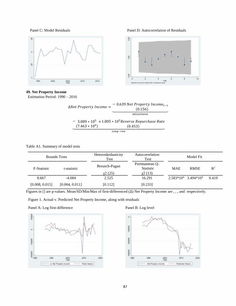
87
Panel C: Model Residuals Panel D: Autocorrelation of Residuals
49. Net Property Income
Estimation Period: 1990 – 2016
∆𝑁𝑒𝑡 𝑃𝑟𝑜𝑝𝑒𝑟𝑡𝑦 𝐼𝑛𝑐𝑜𝑚𝑒 =− 0.639 𝑁𝑒𝑡 𝑃𝑟𝑜𝑝𝑒𝑟𝑡𝑦 𝐼𝑛𝑐𝑜𝑚𝑒𝑡−1
(0.156)⏟ 𝐴𝑑𝑗𝑢𝑠𝑡𝑚𝑒𝑛𝑡
− 3.089 ∗ 105
(7.463 ∗ 104)+1.805 ∗ 105𝑅𝑒𝑣𝑒𝑟𝑠𝑒 𝑅𝑒𝑝𝑢𝑟𝑐ℎ𝑎𝑠𝑒 𝑅𝑎𝑡𝑒
(0.453)⏟ 𝐿𝑜𝑛𝑔−𝑟𝑢𝑛
Table A1. Summary of model tests
Bounds Tests Hetoroskedasticity
Test Autocorrelation
Test Model Fit
F-Statistic t-statistic Breusch-Pagan Portmanteau Q-
Statistic MAE RMSE R2
χ2 (25) χ2 (13)
8.667 -4.084 2.525 16.291 2.583*104 3.494*104 0.419
[0.008, 0.015] [0.004, 0.011] [0.112] [0.233]
Figures in [] are p-values. Mean/SD/Min/Max of first-differenced (∆) Net Property Income are , , , and respectively.
Figure 1. Actual v. Predicted Net Property Income, along with residuals
Panel A: Log first-difference Panel B: Log level
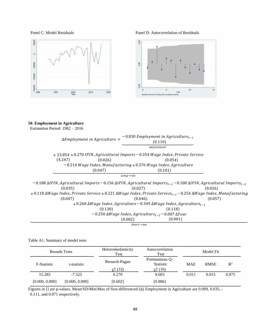
88
Panel C: Model Residuals Panel D: Autocorrelation of Residuals
50. Employment in Agriculture
Estimation Period: 1982 – 2016
∆𝐸𝑚𝑝𝑙𝑜𝑦𝑚𝑒𝑛𝑡 𝑖𝑛 𝐴𝑔𝑟𝑖𝑐𝑢𝑙𝑡𝑢𝑟𝑒 =−0.830 𝐸𝑚𝑝𝑙𝑜𝑦𝑚𝑒𝑛𝑡 𝑖𝑛 𝐴𝑔𝑟𝑖𝑐𝑢𝑙𝑡𝑢𝑟𝑒𝑡−1
(0.110)⏟ 𝐴𝑑𝑗𝑢𝑠𝑡𝑚𝑒𝑛𝑡
+ 23.854(4.247)
+0.270 𝐼𝑃𝐼𝑁, 𝐴𝑔𝑟𝑖𝑐𝑢𝑙𝑡𝑢𝑟𝑎𝑙 𝐼𝑚𝑝𝑜𝑟𝑡𝑠
(0.026)
−0.354 𝑊𝑎𝑔𝑒 𝐼𝑛𝑑𝑒𝑥, 𝑃𝑟𝑖𝑣𝑎𝑡𝑒 𝑆𝑒𝑟𝑣𝑖𝑐𝑒
(0.054)−0.214 𝑊𝑎𝑔𝑒 𝐼𝑛𝑑𝑒𝑥,𝑀𝑎𝑛𝑢𝑓𝑎𝑐𝑡𝑢𝑟𝑖𝑛𝑔
(0.047)+0.376 𝑊𝑎𝑔𝑒 𝐼𝑛𝑑𝑒𝑥, 𝐴𝑔𝑟𝑖𝑐𝑢𝑙𝑡𝑢𝑟𝑒
(0.101)⏟ 𝐿𝑜𝑛𝑔−𝑟𝑢𝑛
−0.188 ∆𝐼𝑃𝐼𝑁, 𝐴𝑔𝑟𝑖𝑐𝑢𝑙𝑡𝑢𝑟𝑎𝑙 𝐼𝑚𝑝𝑜𝑟𝑡𝑠
(0.035)
−0.156 ∆𝐼𝑃𝐼𝑁, 𝐴𝑔𝑟𝑖𝑐𝑢𝑙𝑡𝑢𝑟𝑎𝑙 𝐼𝑚𝑝𝑜𝑟𝑡𝑠𝑡−1(0.027)
−0.108 ∆𝐼𝑃𝐼𝑁, 𝐴𝑔𝑟𝑖𝑐𝑢𝑙𝑡𝑢𝑟𝑎𝑙 𝐼𝑚𝑝𝑜𝑟𝑡𝑠𝑡−2(0.026)
+0.118 ∆𝑊𝑎𝑔𝑒 𝐼𝑛𝑑𝑒𝑥, 𝑃𝑟𝑖𝑣𝑎𝑡𝑒 𝑆𝑒𝑟𝑣𝑖𝑐𝑒
(0.047)+0.221 ∆𝑊𝑎𝑔𝑒 𝐼𝑛𝑑𝑒𝑥, 𝑃𝑟𝑖𝑣𝑎𝑡𝑒 𝑆𝑒𝑟𝑣𝑖𝑐𝑒𝑡−1
(0.046)
−0.254 ∆𝑊𝑎𝑔𝑒 𝐼𝑛𝑑𝑒𝑥,𝑀𝑎𝑛𝑢𝑓𝑎𝑐𝑡𝑢𝑟𝑖𝑛𝑔
(0.057)
+0.260 ∆𝑊𝑎𝑔𝑒 𝐼𝑛𝑑𝑒𝑥, 𝐴𝑔𝑟𝑖𝑐𝑢𝑙𝑡𝑢𝑟𝑒
(0.130)
−0.349 ∆𝑊𝑎𝑔𝑒 𝐼𝑛𝑑𝑒𝑥, 𝐴𝑔𝑟𝑖𝑐𝑢𝑙𝑡𝑢𝑟𝑒𝑡−1(0.118)
−0.250 ∆𝑊𝑎𝑔𝑒 𝐼𝑛𝑑𝑒𝑥, 𝐴𝑔𝑟𝑖𝑐𝑢𝑙𝑡𝑢𝑟𝑒𝑡−2(0.082)
−0.007 ∆𝑌𝑒𝑎𝑟(0.001)⏟
𝑆ℎ𝑜𝑟𝑡−𝑟𝑢𝑛
Table A1. Summary of model tests
Bounds Tests Hetoroskedasticity
Test Autocorrelation
Test Model Fit
F-Statistic t-statistic Breusch-Pagan Portmanteau Q-
Statistic MAE RMSE R2
χ2 (33) χ2 (16)
15.283 -7.525 0.270 9.603 0.011 0.015 0.875
[0.000, 0.000] [0.000, 0.000] [0.602] [0.886]
Figures in [] are p-values. Mean/SD/Min/Max of first-differenced (∆) Employment in Agriculture are 0.009, 0.035, -
0.111, and 0.071 respectively.
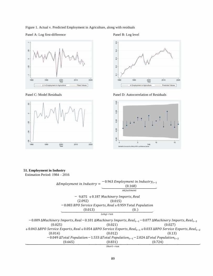
89
Figure 1. Actual v. Predicted Employment in Agriculture, along with residuals
Panel A: Log first-difference Panel B: Log level
Panel C: Model Residuals Panel D: Autocorrelation of Residuals
51. Employment in Industry
Estimation Period: 1984 – 2016
∆𝐸𝑚𝑝𝑙𝑜𝑦𝑚𝑒𝑛𝑡 𝑖𝑛 𝐼𝑛𝑑𝑢𝑠𝑡𝑟𝑦 =−0.963 𝐸𝑚𝑝𝑙𝑜𝑦𝑚𝑒𝑛𝑡 𝑖𝑛 𝐼𝑛𝑑𝑢𝑠𝑡𝑟𝑦𝑡−1
(0.168)⏟ 𝐴𝑑𝑗𝑢𝑠𝑡𝑚𝑒𝑛𝑡
− 9.875(2.092)
+0.187 𝑀𝑎𝑐ℎ𝑖𝑛𝑒𝑟𝑦 𝐼𝑚𝑝𝑜𝑟𝑡𝑠, 𝑅𝑒𝑎𝑙(0.015)
−0.083 𝐵𝑃𝑂 𝑆𝑒𝑟𝑣𝑖𝑐𝑒 𝐸𝑥𝑝𝑜𝑟𝑡𝑠, 𝑅𝑒𝑎𝑙(0.013)
+0.959 𝑇𝑜𝑡𝑎𝑙 𝑃𝑜𝑝𝑢𝑙𝑎𝑡𝑖𝑜𝑛(0. )⏟
𝐿𝑜𝑛𝑔−𝑟𝑢𝑛
−0.009 ∆𝑀𝑎𝑐ℎ𝑖𝑛𝑒𝑟𝑦 𝐼𝑚𝑝𝑜𝑟𝑡𝑠, 𝑅𝑒𝑎𝑙
(0.025)
−0.101 ∆𝑀𝑎𝑐ℎ𝑖𝑛𝑒𝑟𝑦 𝐼𝑚𝑝𝑜𝑟𝑡𝑠, 𝑅𝑒𝑎𝑙𝑡−1(0.021)
−0.077 ∆𝑀𝑎𝑐ℎ𝑖𝑛𝑒𝑟𝑦 𝐼𝑚𝑝𝑜𝑟𝑡𝑠, 𝑅𝑒𝑎𝑙𝑡−2(0.027)
+0.043 ∆𝐵𝑃𝑂 𝑆𝑒𝑟𝑣𝑖𝑐𝑒 𝐸𝑥𝑝𝑜𝑟𝑡𝑠, 𝑅𝑒𝑎𝑙(0.014)
+0.054 ∆𝐵𝑃𝑂 𝑆𝑒𝑟𝑣𝑖𝑐𝑒 𝐸𝑥𝑝𝑜𝑟𝑡𝑠, 𝑅𝑒𝑎𝑙𝑡−1(0.012)
+0.033 ∆𝐵𝑃𝑂 𝑆𝑒𝑟𝑣𝑖𝑐𝑒 𝐸𝑥𝑝𝑜𝑟𝑡𝑠, 𝑅𝑒𝑎𝑙𝑡−2(0.13)
−0.049 ∆𝑇𝑜𝑡𝑎𝑙 𝑃𝑜𝑝𝑢𝑙𝑎𝑡𝑖𝑜𝑛(0.665)
−1.533 ∆𝑇𝑜𝑡𝑎𝑙 𝑃𝑜𝑝𝑢𝑙𝑎𝑡𝑖𝑜𝑛𝑡−1(0.831)
−2.024 ∆𝑇𝑜𝑡𝑎𝑙 𝑃𝑜𝑝𝑢𝑙𝑎𝑡𝑖𝑜𝑛𝑡−2(0.724)⏟
𝑆ℎ𝑜𝑟𝑡−𝑟𝑢𝑛
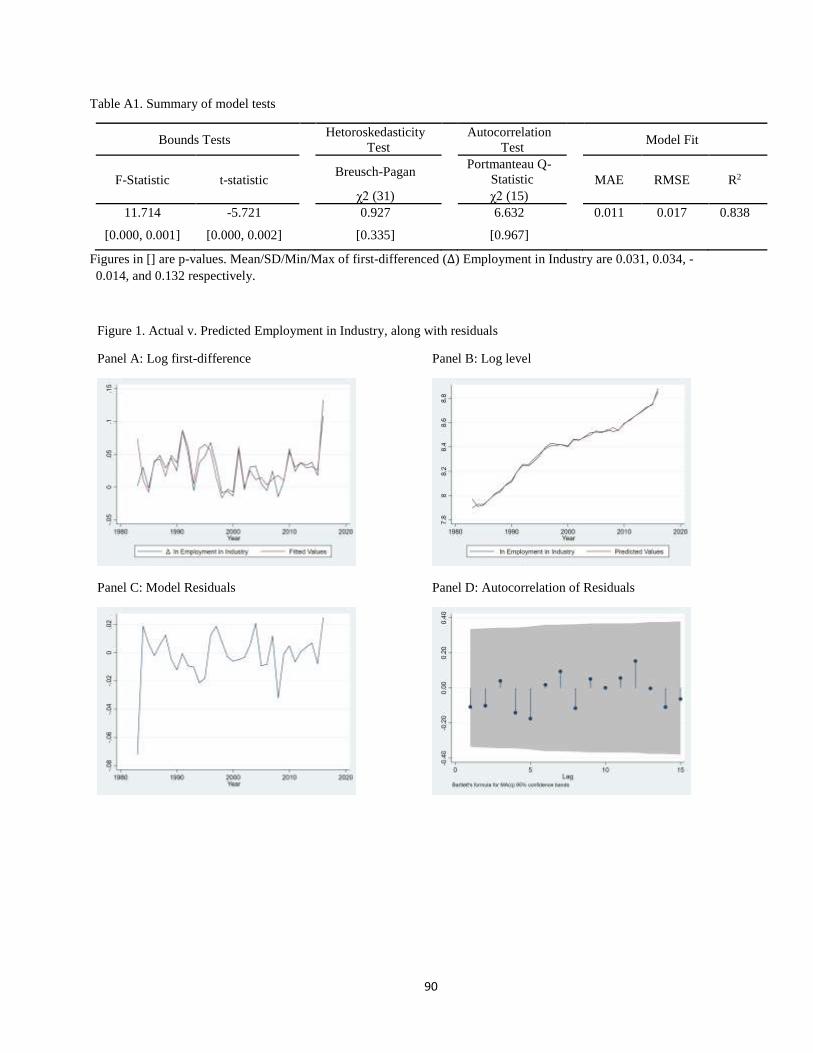
90
Table A1. Summary of model tests
Bounds Tests Hetoroskedasticity
Test Autocorrelation
Test Model Fit
F-Statistic t-statistic Breusch-Pagan Portmanteau Q-
Statistic MAE RMSE R2
χ2 (31) χ2 (15)
11.714 -5.721 0.927 6.632 0.011 0.017 0.838
[0.000, 0.001] [0.000, 0.002] [0.335] [0.967]
Figures in [] are p-values. Mean/SD/Min/Max of first-differenced (∆) Employment in Industry are 0.031, 0.034, -
0.014, and 0.132 respectively.
Figure 1. Actual v. Predicted Employment in Industry, along with residuals
Panel A: Log first-difference Panel B: Log level
Panel C: Model Residuals Panel D: Autocorrelation of Residuals
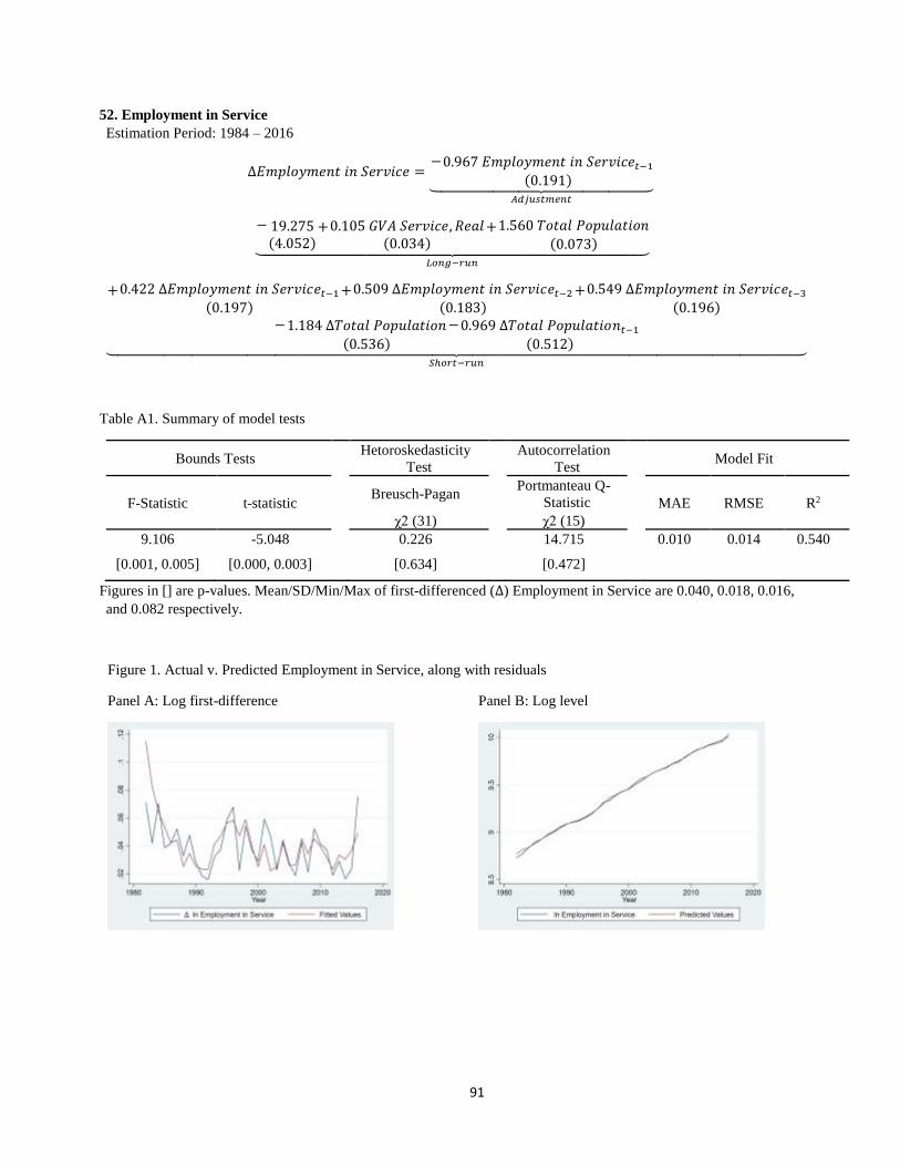
91
52. Employment in Service
Estimation Period: 1984 – 2016
∆𝐸𝑚𝑝𝑙𝑜𝑦𝑚𝑒𝑛𝑡 𝑖𝑛 𝑆𝑒𝑟𝑣𝑖𝑐𝑒 =−0.967 𝐸𝑚𝑝𝑙𝑜𝑦𝑚𝑒𝑛𝑡 𝑖𝑛 𝑆𝑒𝑟𝑣𝑖𝑐𝑒𝑡−1
(0.191)⏟ 𝐴𝑑𝑗𝑢𝑠𝑡𝑚𝑒𝑛𝑡
− 19.275(4.052)
+0.105 𝐺𝑉𝐴 𝑆𝑒𝑟𝑣𝑖𝑐𝑒, 𝑅𝑒𝑎𝑙(0.034)
+1.560 𝑇𝑜𝑡𝑎𝑙 𝑃𝑜𝑝𝑢𝑙𝑎𝑡𝑖𝑜𝑛(0.073)⏟
𝐿𝑜𝑛𝑔−𝑟𝑢𝑛
+0.422 ∆𝐸𝑚𝑝𝑙𝑜𝑦𝑚𝑒𝑛𝑡 𝑖𝑛 𝑆𝑒𝑟𝑣𝑖𝑐𝑒𝑡−1(0.197)
+0.509 ∆𝐸𝑚𝑝𝑙𝑜𝑦𝑚𝑒𝑛𝑡 𝑖𝑛 𝑆𝑒𝑟𝑣𝑖𝑐𝑒𝑡−2(0.183)
+0.549 ∆𝐸𝑚𝑝𝑙𝑜𝑦𝑚𝑒𝑛𝑡 𝑖𝑛 𝑆𝑒𝑟𝑣𝑖𝑐𝑒𝑡−3(0.196)
−1.184 ∆𝑇𝑜𝑡𝑎𝑙 𝑃𝑜𝑝𝑢𝑙𝑎𝑡𝑖𝑜𝑛(0.536)
−0.969 ∆𝑇𝑜𝑡𝑎𝑙 𝑃𝑜𝑝𝑢𝑙𝑎𝑡𝑖𝑜𝑛𝑡−1(0.512)⏟
𝑆ℎ𝑜𝑟𝑡−𝑟𝑢𝑛
Table A1. Summary of model tests
Bounds Tests Hetoroskedasticity
Test Autocorrelation
Test Model Fit
F-Statistic t-statistic Breusch-Pagan Portmanteau Q-
Statistic MAE RMSE R2
χ2 (31) χ2 (15)
9.106 -5.048 0.226 14.715 0.010 0.014 0.540
[0.001, 0.005] [0.000, 0.003] [0.634] [0.472]
Figures in [] are p-values. Mean/SD/Min/Max of first-differenced (∆) Employment in Service are 0.040, 0.018, 0.016,
and 0.082 respectively.
Figure 1. Actual v. Predicted Employment in Service, along with residuals
Panel A: Log first-difference Panel B: Log level
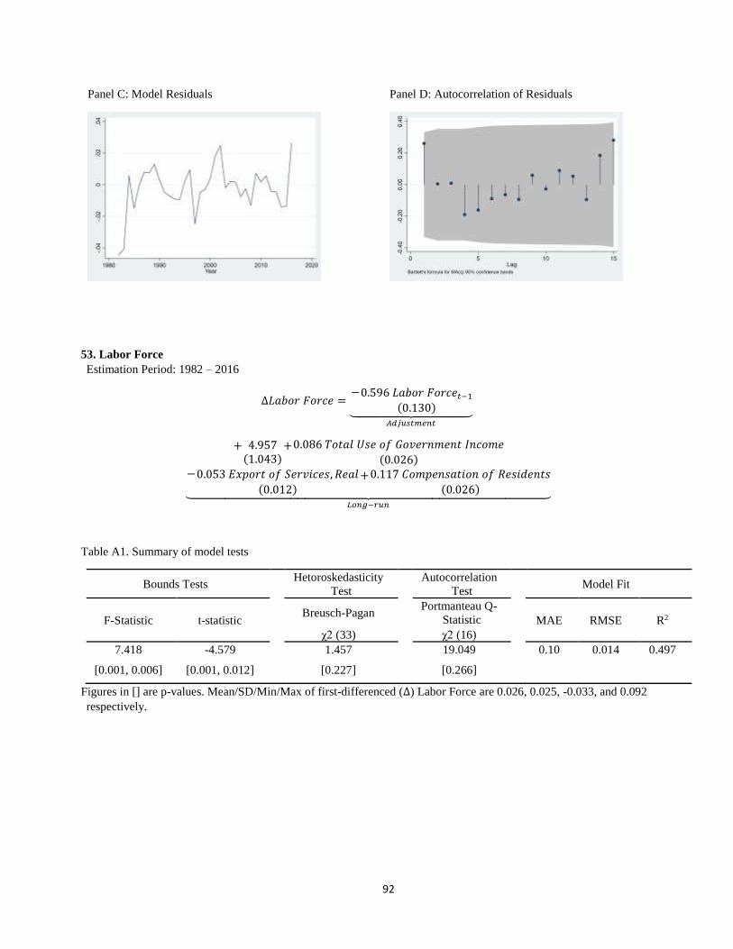
92
Panel C: Model Residuals Panel D: Autocorrelation of Residuals
53. Labor Force
Estimation Period: 1982 – 2016
∆𝐿𝑎𝑏𝑜𝑟 𝐹𝑜𝑟𝑐𝑒 =−0.596 𝐿𝑎𝑏𝑜𝑟 𝐹𝑜𝑟𝑐𝑒𝑡−1
(0.130)⏟ 𝐴𝑑𝑗𝑢𝑠𝑡𝑚𝑒𝑛𝑡
+ 4.957(1.043)
+0.086 𝑇𝑜𝑡𝑎𝑙 𝑈𝑠𝑒 𝑜𝑓 𝐺𝑜𝑣𝑒𝑟𝑛𝑚𝑒𝑛𝑡 𝐼𝑛𝑐𝑜𝑚𝑒
(0.026)−0.053 𝐸𝑥𝑝𝑜𝑟𝑡 𝑜𝑓 𝑆𝑒𝑟𝑣𝑖𝑐𝑒𝑠, 𝑅𝑒𝑎𝑙
(0.012)+0.117 𝐶𝑜𝑚𝑝𝑒𝑛𝑠𝑎𝑡𝑖𝑜𝑛 𝑜𝑓 𝑅𝑒𝑠𝑖𝑑𝑒𝑛𝑡𝑠
(0.026)⏟ 𝐿𝑜𝑛𝑔−𝑟𝑢𝑛
Table A1. Summary of model tests
Bounds Tests Hetoroskedasticity
Test Autocorrelation
Test Model Fit
F-Statistic t-statistic Breusch-Pagan Portmanteau Q-
Statistic MAE RMSE R2
χ2 (33) χ2 (16)
7.418 -4.579 1.457 19.049 0.10 0.014 0.497
[0.001, 0.006] [0.001, 0.012] [0.227] [0.266]
Figures in [] are p-values. Mean/SD/Min/Max of first-differenced (∆) Labor Force are 0.026, 0.025, -0.033, and 0.092
respectively.
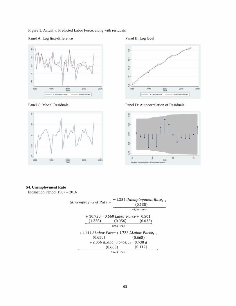
93
Figure 1. Actual v. Predicted Labor Force, along with residuals
Panel A: Log first-difference Panel B: Log level
Panel C: Model Residuals Panel D: Autocorrelation of Residuals
54. Unemployment Rate
Estimation Period: 1967 – 2016
∆𝑈𝑛𝑒𝑚𝑝𝑙𝑜𝑦𝑚𝑒𝑛𝑡 𝑅𝑎𝑡𝑒 =−1.354 𝑈𝑛𝑒𝑚𝑝𝑙𝑜𝑦𝑚𝑒𝑛𝑡 𝑅𝑎𝑡𝑒𝑡−1
(0.135)⏟ 𝐴𝑑𝑗𝑢𝑠𝑡𝑚𝑒𝑛𝑡
+ 10.720(1.228)
−0.660 𝐿𝑎𝑏𝑜𝑟 𝐹𝑜𝑟𝑐𝑒(0.056)
+ 0.501(0.033)⏟
𝐿𝑜𝑛𝑔−𝑟𝑢𝑛
+1.144 ∆𝐿𝑎𝑏𝑜𝑟 𝐹𝑜𝑟𝑐𝑒(0.650)
+1.738 ∆𝐿𝑎𝑏𝑜𝑟 𝐹𝑜𝑟𝑐𝑒𝑡−1(0.665)
+2.056 ∆𝐿𝑎𝑏𝑜𝑟 𝐹𝑜𝑟𝑐𝑒𝑡−2(0.663)
−0.430 ∆(0.112)⏟
𝑆ℎ𝑜𝑟𝑡−𝑟𝑢𝑛

94
Table A1. Summary of model tests
Bounds Tests Hetoroskedasticity
Test Autocorrelation
Test Model Fit
F-Statistic t-statistic Breusch-Pagan Portmanteau Q-
Statistic MAE RMSE R2
χ2 (48) χ2 (24)
33.846 -10.014 0.042 12.238 0.079 0.109 0.718
[0.000, 0.000] [0.000, 0.000] [0.837] [0.977]
Figures in [] are p-values. Mean/SD/Min/Max of first-differenced (∆) Unemployment Rate are -0.004, 0.190, -0.584,
and 0.531 respectively.
Figure 1. Actual v. Predicted Unemployment Rate, along with residuals
Panel A: Log first-difference Panel B: Log level
Panel C: Model Residuals Panel D: Autocorrelation of Residuals
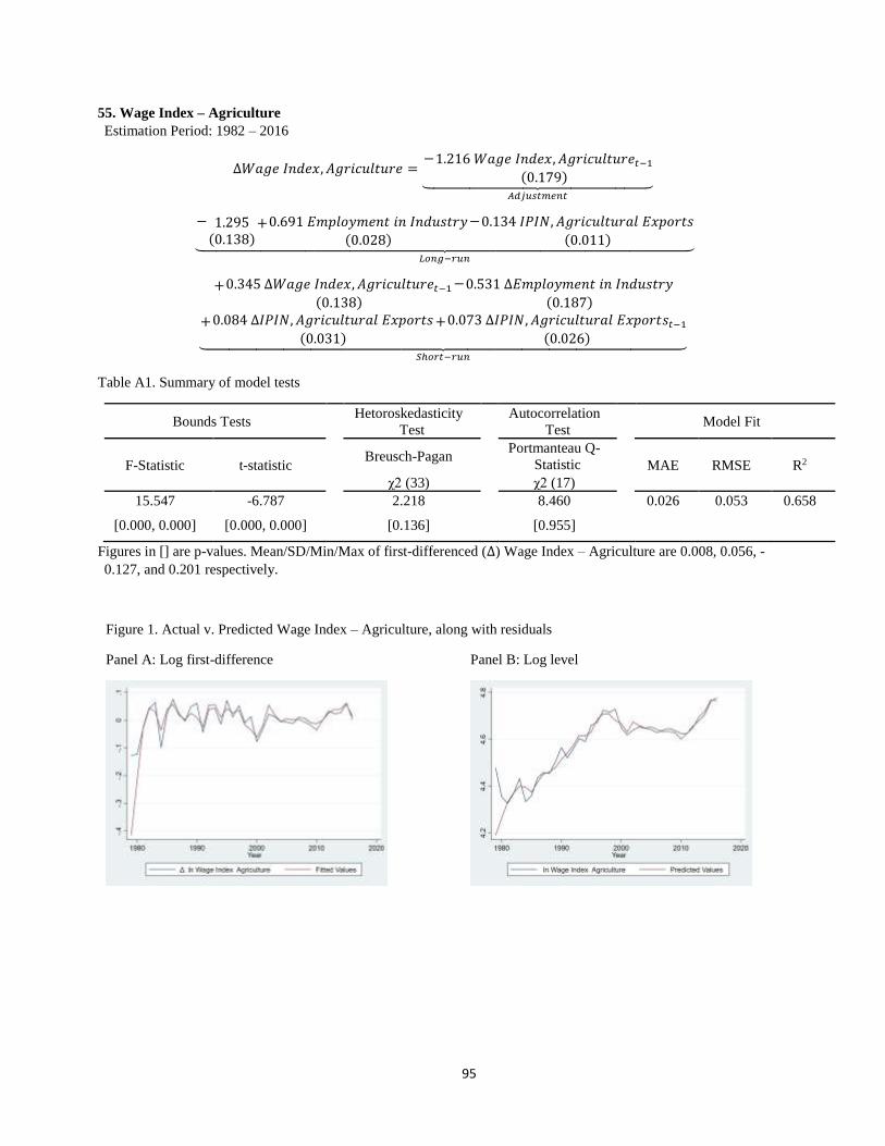
95
55. Wage Index – Agriculture
Estimation Period: 1982 – 2016
∆𝑊𝑎𝑔𝑒 𝐼𝑛𝑑𝑒𝑥, 𝐴𝑔𝑟𝑖𝑐𝑢𝑙𝑡𝑢𝑟𝑒 =−1.216 𝑊𝑎𝑔𝑒 𝐼𝑛𝑑𝑒𝑥, 𝐴𝑔𝑟𝑖𝑐𝑢𝑙𝑡𝑢𝑟𝑒𝑡−1
(0.179)⏟ 𝐴𝑑𝑗𝑢𝑠𝑡𝑚𝑒𝑛𝑡
− 1.295(0.138)
+0.691 𝐸𝑚𝑝𝑙𝑜𝑦𝑚𝑒𝑛𝑡 𝑖𝑛 𝐼𝑛𝑑𝑢𝑠𝑡𝑟𝑦(0.028)
−0.134 𝐼𝑃𝐼𝑁, 𝐴𝑔𝑟𝑖𝑐𝑢𝑙𝑡𝑢𝑟𝑎𝑙 𝐸𝑥𝑝𝑜𝑟𝑡𝑠
(0.011)⏟ 𝐿𝑜𝑛𝑔−𝑟𝑢𝑛
+0.345 ∆𝑊𝑎𝑔𝑒 𝐼𝑛𝑑𝑒𝑥, 𝐴𝑔𝑟𝑖𝑐𝑢𝑙𝑡𝑢𝑟𝑒𝑡−1(0.138)
−0.531 ∆𝐸𝑚𝑝𝑙𝑜𝑦𝑚𝑒𝑛𝑡 𝑖𝑛 𝐼𝑛𝑑𝑢𝑠𝑡𝑟𝑦
(0.187)
+0.084 ∆𝐼𝑃𝐼𝑁, 𝐴𝑔𝑟𝑖𝑐𝑢𝑙𝑡𝑢𝑟𝑎𝑙 𝐸𝑥𝑝𝑜𝑟𝑡𝑠
(0.031)+0.073 ∆𝐼𝑃𝐼𝑁, 𝐴𝑔𝑟𝑖𝑐𝑢𝑙𝑡𝑢𝑟𝑎𝑙 𝐸𝑥𝑝𝑜𝑟𝑡𝑠𝑡−1
(0.026)⏟ 𝑆ℎ𝑜𝑟𝑡−𝑟𝑢𝑛
Table A1. Summary of model tests
Bounds Tests Hetoroskedasticity
Test Autocorrelation
Test Model Fit
F-Statistic t-statistic Breusch-Pagan Portmanteau Q-
Statistic MAE RMSE R2
χ2 (33) χ2 (17)
15.547 -6.787 2.218 8.460 0.026 0.053 0.658
[0.000, 0.000] [0.000, 0.000] [0.136] [0.955]
Figures in [] are p-values. Mean/SD/Min/Max of first-differenced (∆) Wage Index – Agriculture are 0.008, 0.056, -
0.127, and 0.201 respectively.
Figure 1. Actual v. Predicted Wage Index – Agriculture, along with residuals
Panel A: Log first-difference Panel B: Log level
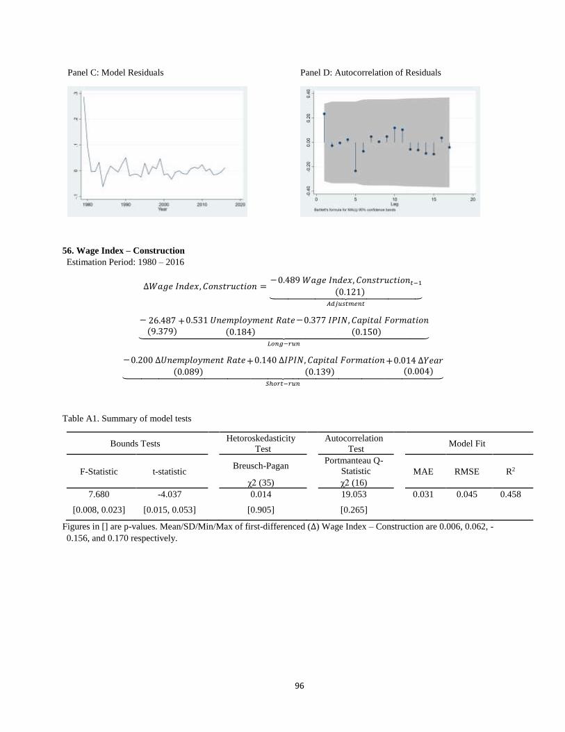
96
Panel C: Model Residuals Panel D: Autocorrelation of Residuals
56. Wage Index – Construction
Estimation Period: 1980 – 2016
∆𝑊𝑎𝑔𝑒 𝐼𝑛𝑑𝑒𝑥, 𝐶𝑜𝑛𝑠𝑡𝑟𝑢𝑐𝑡𝑖𝑜𝑛 =−0.489 𝑊𝑎𝑔𝑒 𝐼𝑛𝑑𝑒𝑥, 𝐶𝑜𝑛𝑠𝑡𝑟𝑢𝑐𝑡𝑖𝑜𝑛𝑡−1
(0.121)⏟ 𝐴𝑑𝑗𝑢𝑠𝑡𝑚𝑒𝑛𝑡
− 26.487(9.379)
+0.531 𝑈𝑛𝑒𝑚𝑝𝑙𝑜𝑦𝑚𝑒𝑛𝑡 𝑅𝑎𝑡𝑒(0.184)
−0.377 𝐼𝑃𝐼𝑁, 𝐶𝑎𝑝𝑖𝑡𝑎𝑙 𝐹𝑜𝑟𝑚𝑎𝑡𝑖𝑜𝑛(0.150)⏟
𝐿𝑜𝑛𝑔−𝑟𝑢𝑛
−0.200 ∆𝑈𝑛𝑒𝑚𝑝𝑙𝑜𝑦𝑚𝑒𝑛𝑡 𝑅𝑎𝑡𝑒(0.089)
+0.140 ∆𝐼𝑃𝐼𝑁, 𝐶𝑎𝑝𝑖𝑡𝑎𝑙 𝐹𝑜𝑟𝑚𝑎𝑡𝑖𝑜𝑛(0.139)
+0.014 ∆𝑌𝑒𝑎𝑟(0.004)⏟
𝑆ℎ𝑜𝑟𝑡−𝑟𝑢𝑛
Table A1. Summary of model tests
Bounds Tests Hetoroskedasticity
Test Autocorrelation
Test Model Fit
F-Statistic t-statistic Breusch-Pagan Portmanteau Q-
Statistic MAE RMSE R2
χ2 (35) χ2 (16)
7.680 -4.037 0.014 19.053 0.031 0.045 0.458
[0.008, 0.023] [0.015, 0.053] [0.905] [0.265]
Figures in [] are p-values. Mean/SD/Min/Max of first-differenced (∆) Wage Index – Construction are 0.006, 0.062, -
0.156, and 0.170 respectively.
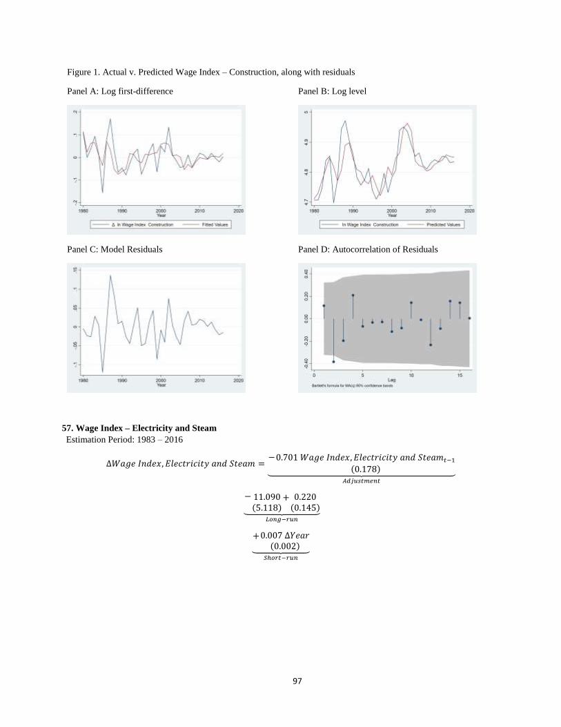
97
Figure 1. Actual v. Predicted Wage Index – Construction, along with residuals
Panel A: Log first-difference Panel B: Log level
Panel C: Model Residuals Panel D: Autocorrelation of Residuals
57. Wage Index – Electricity and Steam
Estimation Period: 1983 – 2016
∆𝑊𝑎𝑔𝑒 𝐼𝑛𝑑𝑒𝑥, 𝐸𝑙𝑒𝑐𝑡𝑟𝑖𝑐𝑖𝑡𝑦 𝑎𝑛𝑑 𝑆𝑡𝑒𝑎𝑚 =−0.701 𝑊𝑎𝑔𝑒 𝐼𝑛𝑑𝑒𝑥, 𝐸𝑙𝑒𝑐𝑡𝑟𝑖𝑐𝑖𝑡𝑦 𝑎𝑛𝑑 𝑆𝑡𝑒𝑎𝑚𝑡−1
(0.178)⏟ 𝐴𝑑𝑗𝑢𝑠𝑡𝑚𝑒𝑛𝑡
− 11.090(5.118)
+ 0.220(0.145)⏟
𝐿𝑜𝑛𝑔−𝑟𝑢𝑛
+0.007 ∆𝑌𝑒𝑎𝑟(0.002)⏟
𝑆ℎ𝑜𝑟𝑡−𝑟𝑢𝑛
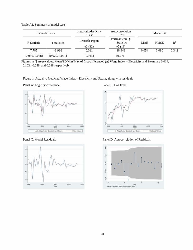
98
Table A1. Summary of model tests
Bounds Tests Hetoroskedasticity
Test Autocorrelation
Test Model Fit
F-Statistic t-statistic Breusch-Pagan Portmanteau Q-
Statistic MAE RMSE R2
χ2 (32) χ2 (16)
7.785 -3.936 0.011 18.949 0.054 0.080 0.342
[0.036, 0.058] [0.020, 0.041] [0.914] [0.271]
Figures in [] are p-values. Mean/SD/Min/Max of first-differenced (∆) Wage Index – Electricity and Steam are 0.014,
0.103, -0.259, and 0.248 respectively.
Figure 1. Actual v. Predicted Wage Index – Electricity and Steam, along with residuals
Panel A: Log first-difference Panel B: Log level
Panel C: Model Residuals Panel D: Autocorrelation of Residuals
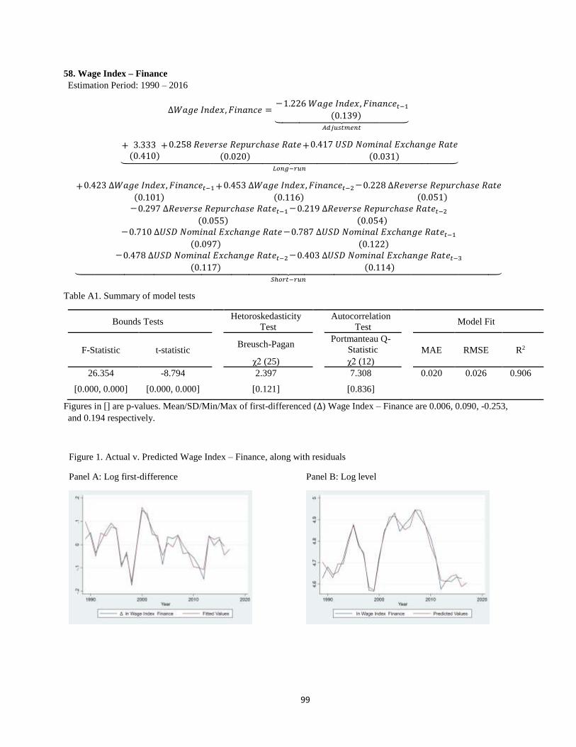
99
58. Wage Index – Finance
Estimation Period: 1990 – 2016
∆𝑊𝑎𝑔𝑒 𝐼𝑛𝑑𝑒𝑥, 𝐹𝑖𝑛𝑎𝑛𝑐𝑒 =−1.226 𝑊𝑎𝑔𝑒 𝐼𝑛𝑑𝑒𝑥, 𝐹𝑖𝑛𝑎𝑛𝑐𝑒𝑡−1
(0.139)⏟ 𝐴𝑑𝑗𝑢𝑠𝑡𝑚𝑒𝑛𝑡
+ 3.333(0.410)
+0.258 𝑅𝑒𝑣𝑒𝑟𝑠𝑒 𝑅𝑒𝑝𝑢𝑟𝑐ℎ𝑎𝑠𝑒 𝑅𝑎𝑡𝑒(0.020)
+0.417 𝑈𝑆𝐷 𝑁𝑜𝑚𝑖𝑛𝑎𝑙 𝐸𝑥𝑐ℎ𝑎𝑛𝑔𝑒 𝑅𝑎𝑡𝑒
(0.031)⏟ 𝐿𝑜𝑛𝑔−𝑟𝑢𝑛
+0.423 ∆𝑊𝑎𝑔𝑒 𝐼𝑛𝑑𝑒𝑥, 𝐹𝑖𝑛𝑎𝑛𝑐𝑒𝑡−1(0.101)
+0.453 ∆𝑊𝑎𝑔𝑒 𝐼𝑛𝑑𝑒𝑥, 𝐹𝑖𝑛𝑎𝑛𝑐𝑒𝑡−2(0.116)
−0.228 ∆𝑅𝑒𝑣𝑒𝑟𝑠𝑒 𝑅𝑒𝑝𝑢𝑟𝑐ℎ𝑎𝑠𝑒 𝑅𝑎𝑡𝑒(0.051)
−0.297 ∆𝑅𝑒𝑣𝑒𝑟𝑠𝑒 𝑅𝑒𝑝𝑢𝑟𝑐ℎ𝑎𝑠𝑒 𝑅𝑎𝑡𝑒𝑡−1(0.055)
−0.219 ∆𝑅𝑒𝑣𝑒𝑟𝑠𝑒 𝑅𝑒𝑝𝑢𝑟𝑐ℎ𝑎𝑠𝑒 𝑅𝑎𝑡𝑒𝑡−2(0.054)
−0.710 ∆𝑈𝑆𝐷 𝑁𝑜𝑚𝑖𝑛𝑎𝑙 𝐸𝑥𝑐ℎ𝑎𝑛𝑔𝑒 𝑅𝑎𝑡𝑒
(0.097)
−0.787 ∆𝑈𝑆𝐷 𝑁𝑜𝑚𝑖𝑛𝑎𝑙 𝐸𝑥𝑐ℎ𝑎𝑛𝑔𝑒 𝑅𝑎𝑡𝑒𝑡−1(0.122)
−0.478 ∆𝑈𝑆𝐷 𝑁𝑜𝑚𝑖𝑛𝑎𝑙 𝐸𝑥𝑐ℎ𝑎𝑛𝑔𝑒 𝑅𝑎𝑡𝑒𝑡−2(0.117)
−0.403 ∆𝑈𝑆𝐷 𝑁𝑜𝑚𝑖𝑛𝑎𝑙 𝐸𝑥𝑐ℎ𝑎𝑛𝑔𝑒 𝑅𝑎𝑡𝑒𝑡−3(0.114)⏟
𝑆ℎ𝑜𝑟𝑡−𝑟𝑢𝑛
Table A1. Summary of model tests
Bounds Tests Hetoroskedasticity
Test Autocorrelation
Test Model Fit
F-Statistic t-statistic Breusch-Pagan Portmanteau Q-
Statistic MAE RMSE R2
χ2 (25) χ2 (12)
26.354 -8.794 2.397 7.308 0.020 0.026 0.906
[0.000, 0.000] [0.000, 0.000] [0.121] [0.836]
Figures in [] are p-values. Mean/SD/Min/Max of first-differenced (∆) Wage Index – Finance are 0.006, 0.090, -0.253,
and 0.194 respectively.
Figure 1. Actual v. Predicted Wage Index – Finance, along with residuals
Panel A: Log first-difference Panel B: Log level

100
Panel C: Model Residuals Panel D: Autocorrelation of Residuals
59. Wage Index – Manufacturing
Estimation Period: 1981 – 2016
∆𝑊𝑎𝑔𝑒 𝐼𝑛𝑑𝑒𝑥,𝑀𝑎𝑛𝑢𝑓𝑎𝑐𝑡𝑢𝑟𝑖𝑛𝑔 =−0.413 𝑊𝑎𝑔𝑒 𝐼𝑛𝑑𝑒𝑥,𝑀𝑎𝑛𝑢𝑓𝑎𝑐𝑡𝑢𝑟𝑖𝑛𝑔𝑡−1
(0.087)⏟ 𝐴𝑑𝑗𝑢𝑠𝑡𝑚𝑒𝑛𝑡
+ 1.853(0.388)
+0.390 𝐼𝑃𝐼𝑁,𝑀𝑎𝑡𝑒𝑟𝑖𝑎𝑙𝑠 𝐼𝑚𝑝𝑜𝑟𝑡𝑠(0.138)
−0.942 𝐼𝑃𝐼𝑁,𝑀𝑎𝑐ℎ𝑖𝑛𝑒𝑟𝑦 𝐼𝑚𝑝𝑜𝑟𝑡𝑠(0.215)
−0.119 𝐼𝑃𝐼𝑁, 𝐹𝑢𝑒𝑙 𝐼𝑚𝑝𝑜𝑟𝑡𝑠(0.033)
+0.415 𝐼𝑃𝐼𝑁, 𝐸𝑥𝑝𝑜𝑟𝑡 𝐺𝑜𝑜𝑑𝑠(0.187)⏟
𝐿𝑜𝑛𝑔−𝑟𝑢𝑛
+0.215 ∆𝑊𝑎𝑔𝑒 𝐼𝑛𝑑𝑒𝑥,𝑀𝑎𝑛𝑢𝑓𝑎𝑐𝑡𝑢𝑟𝑖𝑛𝑔𝑡−1(0.129)
−0.306 ∆𝐼𝑃𝐼𝑁,𝑀𝑎𝑡𝑒𝑟𝑖𝑎𝑙𝑠 𝐼𝑚𝑝𝑜𝑟𝑡𝑠(0.080)
−0.105 ∆𝐼𝑃𝐼𝑁, 𝐹𝑢𝑒𝑙 𝐼𝑚𝑝𝑜𝑟𝑡𝑠
(0.045)
−0.074 ∆𝐼𝑃𝐼𝑁, 𝐹𝑢𝑒𝑙 𝐼𝑚𝑝𝑜𝑟𝑡𝑠𝑡−1(0.040)⏟
𝑆ℎ𝑜𝑟𝑡−𝑟𝑢𝑛
Table A1. Summary of model tests
Bounds Tests Hetoroskedasticity
Test Autocorrelation
Test Model Fit
F-Statistic t-statistic Breusch-Pagan Portmanteau Q-
Statistic MAE RMSE R2
χ2 (34) χ2 (16)
7.122 -4.705 0.739 15.076 0.029 0.042 0.678
[0.001, 0.006] [0.001, 0.016] [0.389] [0.519]
Figures in [] are p-values. Mean/SD/Min/Max of first-differenced (∆) Wage Index – Manufacturing are -0.012, 0.074,
-0.226, and 0.234 respectively.

101
Figure 1. Actual v. Predicted Wage Index – Manufacturing, along with residuals
Panel A: Log first-difference Panel B: Log level
Panel C: Model Residuals Panel D: Autocorrelation of Residuals
60. Wage Index – Mining
Estimation Period: 1983 – 2016
∆𝑊𝑎𝑔𝑒 𝐼𝑛𝑑𝑒𝑥,𝑀𝑖𝑛𝑖𝑛𝑔 =−0.529 𝑊𝑎𝑔𝑒 𝐼𝑛𝑑𝑒𝑥,𝑀𝑖𝑛𝑖𝑛𝑔𝑡−1
(0.102)⏟ 𝐴𝑑𝑗𝑢𝑠𝑡𝑚𝑒𝑛𝑡
+ 3.466(0.734)
−0.665 𝑈𝑛𝑒𝑚𝑝𝑙𝑜𝑦𝑚𝑒𝑛𝑡 𝑅𝑎𝑡𝑒(0.158)
+0.468 𝐼𝑃𝐼𝑁 𝑀𝑎𝑐ℎ𝑖𝑛𝑒𝑟𝑦 𝐼𝑚𝑝𝑜𝑟𝑡𝑠(0.047)⏟
𝐿𝑜𝑛𝑔−𝑟𝑢𝑛
+0.074 ∆𝑊𝑎𝑔𝑒 𝐼𝑛𝑑𝑒𝑥,𝑀𝑖𝑛𝑖𝑛𝑔𝑡−1(0.144)
+0.299 ∆𝑊𝑎𝑔𝑒 𝐼𝑛𝑑𝑒𝑥,𝑀𝑖𝑛𝑖𝑛𝑔𝑡−2(0.139)
+0.504 ∆𝑈𝑛𝑒𝑚𝑝𝑙𝑜𝑦𝑚𝑒𝑛𝑡 𝑅𝑎𝑡𝑒
(0.166)
+0.414 ∆𝑈𝑛𝑒𝑚𝑝𝑙𝑜𝑦𝑚𝑒𝑛𝑡 𝑅𝑎𝑡𝑒𝑡−1(0.158)
+0.350 ∆𝑈𝑛𝑒𝑚𝑝𝑙𝑜𝑦𝑚𝑒𝑛𝑡 𝑅𝑎𝑡𝑒𝑡−2(0.152)
−0.095 ∆𝐼𝑃𝐼𝑁 𝑀𝑎𝑐ℎ𝑖𝑛𝑒𝑟𝑦 𝐼𝑚𝑝𝑜𝑟𝑡𝑠
(0.080)
−0.362 ∆𝐼𝑃𝐼𝑁 𝑀𝑎𝑐ℎ𝑖𝑛𝑒𝑟𝑦 𝐼𝑚𝑝𝑜𝑟𝑡𝑠𝑡−1(0.080)⏟
𝑆ℎ𝑜𝑟𝑡−𝑟𝑢𝑛
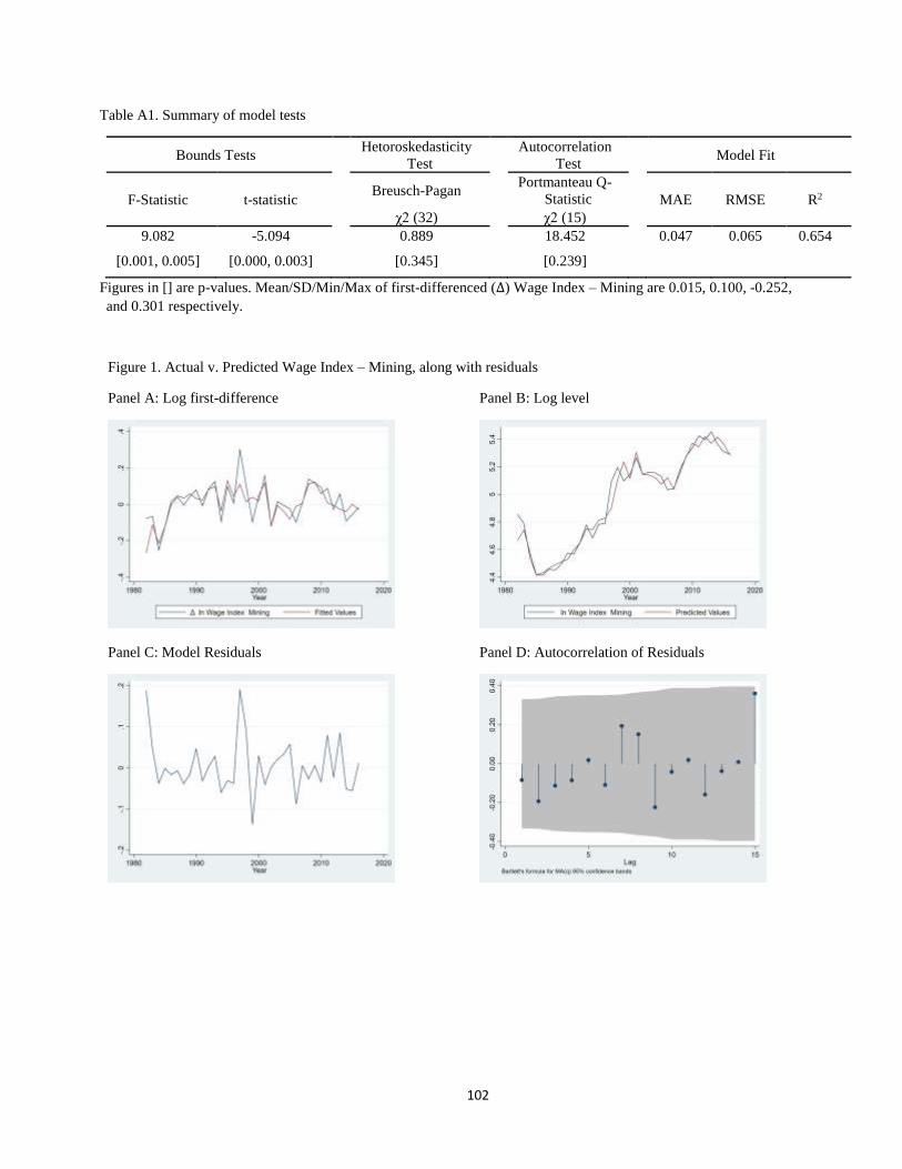
102
Table A1. Summary of model tests
Bounds Tests Hetoroskedasticity
Test Autocorrelation
Test Model Fit
F-Statistic t-statistic Breusch-Pagan Portmanteau Q-
Statistic MAE RMSE R2
χ2 (32) χ2 (15)
9.082 -5.094 0.889 18.452 0.047 0.065 0.654
[0.001, 0.005] [0.000, 0.003] [0.345] [0.239]
Figures in [] are p-values. Mean/SD/Min/Max of first-differenced (∆) Wage Index – Mining are 0.015, 0.100, -0.252,
and 0.301 respectively.
Figure 1. Actual v. Predicted Wage Index – Mining, along with residuals
Panel A: Log first-difference Panel B: Log level
Panel C: Model Residuals Panel D: Autocorrelation of Residuals

103
61. Wage Index – Private Service
Estimation Period: 1983 – 2016
∆𝑊𝑎𝑔𝑒 𝐼𝑛𝑑𝑒𝑥, 𝑃𝑟𝑖𝑣𝑎𝑡𝑒 𝑆𝑒𝑟𝑣𝑖𝑐𝑒 =−0.320 𝑊𝑎𝑔𝑒 𝐼𝑛𝑑𝑒𝑥, 𝑃𝑟𝑖𝑣𝑎𝑡𝑒 𝑆𝑒𝑟𝑣𝑖𝑐𝑒𝑡−1
(0.106)⏟ 𝐴𝑑𝑗𝑢𝑠𝑡𝑚𝑒𝑛𝑡
− 29.775(10.058)
+0.882 𝑈𝑛𝑒𝑚𝑝𝑙𝑜𝑦𝑚𝑒𝑛𝑡 𝑅𝑎𝑡𝑒(0.297)⏟
𝐿𝑜𝑛𝑔−𝑟𝑢𝑛
+0.343 ∆𝑊𝑎𝑔𝑒 𝐼𝑛𝑑𝑒𝑥, 𝑃𝑟𝑖𝑣𝑎𝑡𝑒 𝑆𝑒𝑟𝑣𝑖𝑐𝑒𝑡−1(0.168)
+0.015 ∆𝑌𝑒𝑎𝑟(0.005)⏟
𝑆ℎ𝑜𝑟𝑡−𝑟𝑢𝑛
Table A1. Summary of model tests
Bounds Tests Hetoroskedasticity
Test Autocorrelation
Test Model Fit
F-Statistic t-statistic Breusch-Pagan Portmanteau Q-
Statistic MAE RMSE R2
χ2 (32) χ2 (16)
4.919 -3.015 1.185 12.173 0.049 0.079 0.276
[0.171, 0.241] [0.135, 0.211] [0.276] [0.731]
Figures in [] are p-values. Mean/SD/Min/Max of first-differenced (∆) Wage Index – Private Service are 0.032, 0.084,
-0.106, and 0.437 respectively.
Figure 1. Actual v. Predicted Wage Index – Private Service, along with residuals
Panel A: Log first-difference Panel B: Log level

104
Panel C: Model Residuals Panel D: Autocorrelation of Residuals
62. Wage Index – Real Estate
Estimation Period: 1990 – 2016
∆𝑊𝑎𝑔𝑒 𝐼𝑛𝑑𝑒𝑥, 𝑅𝑒𝑎𝑙 𝐸𝑠𝑡𝑎𝑡𝑒 =−0.884 𝑊𝑎𝑔𝑒 𝐼𝑛𝑑𝑒𝑥, 𝑅𝑒𝑎𝑙 𝐸𝑠𝑡𝑎𝑡𝑒𝑡−1
(0.187)⏟ 𝐴𝑑𝑗𝑢𝑠𝑡𝑚𝑒𝑛𝑡
+ 36.819(12.584)
−0.020 𝑈𝑛𝑒𝑚𝑝𝑙𝑜𝑦𝑚𝑒𝑛𝑡 𝑅𝑎𝑡𝑒
(0.101)−0.392 𝐿𝑒𝑛𝑑𝑖𝑛𝑔 𝑅𝑎𝑡𝑒
(0.133)
−0.178 𝐼𝑃𝐼𝑁, 𝑆𝑒𝑟𝑣𝑖𝑐𝑒 𝐸𝑥𝑝𝑜𝑟𝑡𝑠(0.043)⏟
𝐿𝑜𝑛𝑔−𝑟𝑢𝑛
+0.330 ∆𝐿𝑒𝑛𝑑𝑖𝑛𝑔 𝑅𝑎𝑡𝑒
(0.095)+0.287 ∆𝐿𝑒𝑛𝑑𝑖𝑛𝑔 𝑅𝑎𝑡𝑒𝑡−1
(0.106)+0.016 ∆𝑌𝑒𝑎𝑟
(0.006)⏟ 𝑆ℎ𝑜𝑟𝑡−𝑟𝑢𝑛
Table A1. Summary of model tests
Bounds Tests Hetoroskedasticity
Test Autocorrelation
Test Model Fit
F-Statistic t-statistic Breusch-Pagan Portmanteau Q-
Statistic MAE RMSE R2
χ2 (29) χ2 (15)
6.195 -4.716 0.753 15.777 0.055 0.077 0.545
[0.014, 0.044] [0.004, 0.024] [0.385] [0.396]
Figures in [] are p-values. Mean/SD/Min/Max of first-differenced (∆) Wage Index – Real Estate are -0.010, 0.082, -
0.218, and 0.245 respectively.

105
Figure 1. Actual v. Predicted Wage Index – Real Estate, along with residuals
Panel A: Log first-difference Panel B: Log level
Panel C: Model Residuals Panel D: Autocorrelation of Residuals
63. Wage Index – Trade
Estimation Period: 1983 – 2016
∆𝑊𝑎𝑔𝑒 𝐼𝑛𝑑𝑒𝑥, 𝑇𝑟𝑎𝑑𝑒 =−0.779 𝑊𝑎𝑔𝑒 𝐼𝑛𝑑𝑒𝑥, 𝑇𝑟𝑎𝑑𝑒𝑡−1
(0.201)⏟ 𝐴𝑑𝑗𝑢𝑠𝑡𝑚𝑒𝑛𝑡
+ 4.381(1.173)
+0.140 𝑈𝑛𝑒𝑚𝑝𝑙𝑜𝑦𝑚𝑒𝑛𝑡 𝑅𝑎𝑡𝑒(0.080)
−0.303 𝑊𝑎𝑔𝑒 𝐼𝑛𝑑𝑒𝑥,𝑀𝑎𝑛𝑢𝑓𝑎𝑐𝑡𝑢𝑟𝑖𝑛𝑔
(0.057)⏟ 𝐿𝑜𝑛𝑔−𝑟𝑢𝑛
+0.577 ∆𝑊𝑎𝑔𝑒 𝐼𝑛𝑑𝑒𝑥, 𝑇𝑟𝑎𝑑𝑒𝑡−1(0.164)
+0.420 ∆𝑊𝑎𝑔𝑒 𝐼𝑛𝑑𝑒𝑥, 𝑇𝑟𝑎𝑑𝑒𝑡−2(0.179)
+0.502 ∆𝑊𝑎𝑔𝑒 𝐼𝑛𝑑𝑒𝑥,𝑀𝑎𝑛𝑢𝑓𝑎𝑐𝑡𝑢𝑟𝑖𝑛𝑔
(0.181)⏟ 𝑆ℎ𝑜𝑟𝑡−𝑟𝑢𝑛
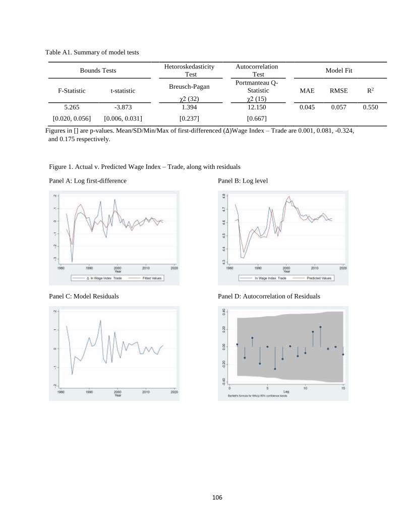
106
Table A1. Summary of model tests
Bounds Tests Hetoroskedasticity
Test Autocorrelation
Test Model Fit
F-Statistic t-statistic Breusch-Pagan Portmanteau Q-
Statistic MAE RMSE R2
χ2 (32) χ2 (15)
5.265 -3.873 1.394 12.150 0.045 0.057 0.550
[0.020, 0.056] [0.006, 0.031] [0.237] [0.667]
Figures in [] are p-values. Mean/SD/Min/Max of first-differenced (∆)Wage Index – Trade are 0.001, 0.081, -0.324,
and 0.175 respectively.
Figure 1. Actual v. Predicted Wage Index – Trade, along with residuals
Panel A: Log first-difference Panel B: Log level
Panel C: Model Residuals Panel D: Autocorrelation of Residuals
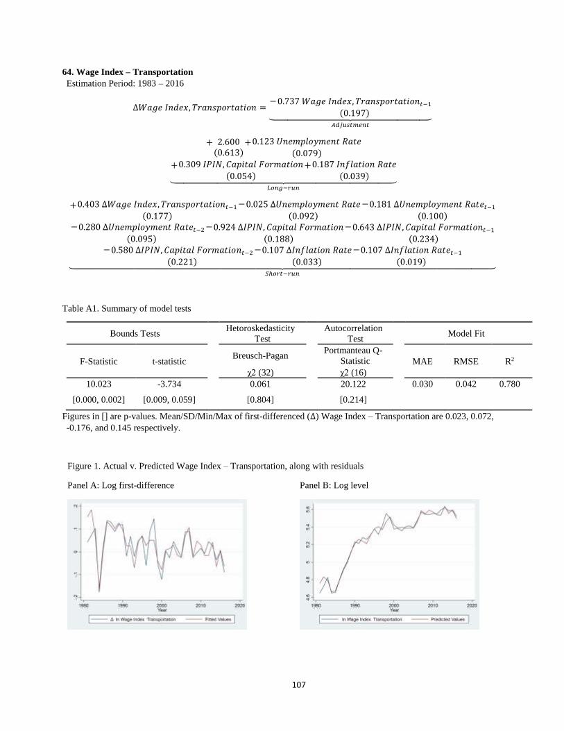
107
64. Wage Index – Transportation
Estimation Period: 1983 – 2016
∆𝑊𝑎𝑔𝑒 𝐼𝑛𝑑𝑒𝑥, 𝑇𝑟𝑎𝑛𝑠𝑝𝑜𝑟𝑡𝑎𝑡𝑖𝑜𝑛 =−0.737 𝑊𝑎𝑔𝑒 𝐼𝑛𝑑𝑒𝑥, 𝑇𝑟𝑎𝑛𝑠𝑝𝑜𝑟𝑡𝑎𝑡𝑖𝑜𝑛𝑡−1
(0.197)⏟ 𝐴𝑑𝑗𝑢𝑠𝑡𝑚𝑒𝑛𝑡
+ 2.600(0.613)
+0.123 𝑈𝑛𝑒𝑚𝑝𝑙𝑜𝑦𝑚𝑒𝑛𝑡 𝑅𝑎𝑡𝑒
(0.079)
+0.309 𝐼𝑃𝐼𝑁, 𝐶𝑎𝑝𝑖𝑡𝑎𝑙 𝐹𝑜𝑟𝑚𝑎𝑡𝑖𝑜𝑛(0.054)
+0.187 𝐼𝑛𝑓𝑙𝑎𝑡𝑖𝑜𝑛 𝑅𝑎𝑡𝑒
(0.039)⏟ 𝐿𝑜𝑛𝑔−𝑟𝑢𝑛
+0.403 ∆𝑊𝑎𝑔𝑒 𝐼𝑛𝑑𝑒𝑥, 𝑇𝑟𝑎𝑛𝑠𝑝𝑜𝑟𝑡𝑎𝑡𝑖𝑜𝑛𝑡−1(0.177)
−0.025 ∆𝑈𝑛𝑒𝑚𝑝𝑙𝑜𝑦𝑚𝑒𝑛𝑡 𝑅𝑎𝑡𝑒
(0.092)
−0.181 ∆𝑈𝑛𝑒𝑚𝑝𝑙𝑜𝑦𝑚𝑒𝑛𝑡 𝑅𝑎𝑡𝑒𝑡−1(0.100)
−0.280 ∆𝑈𝑛𝑒𝑚𝑝𝑙𝑜𝑦𝑚𝑒𝑛𝑡 𝑅𝑎𝑡𝑒𝑡−2(0.095)
−0.924 ∆𝐼𝑃𝐼𝑁, 𝐶𝑎𝑝𝑖𝑡𝑎𝑙 𝐹𝑜𝑟𝑚𝑎𝑡𝑖𝑜𝑛(0.188)
−0.643 ∆𝐼𝑃𝐼𝑁, 𝐶𝑎𝑝𝑖𝑡𝑎𝑙 𝐹𝑜𝑟𝑚𝑎𝑡𝑖𝑜𝑛𝑡−1(0.234)
−0.580 ∆𝐼𝑃𝐼𝑁, 𝐶𝑎𝑝𝑖𝑡𝑎𝑙 𝐹𝑜𝑟𝑚𝑎𝑡𝑖𝑜𝑛𝑡−2(0.221)
−0.107 ∆𝐼𝑛𝑓𝑙𝑎𝑡𝑖𝑜𝑛 𝑅𝑎𝑡𝑒
(0.033)
−0.107 ∆𝐼𝑛𝑓𝑙𝑎𝑡𝑖𝑜𝑛 𝑅𝑎𝑡𝑒𝑡−1(0.019)⏟
𝑆ℎ𝑜𝑟𝑡−𝑟𝑢𝑛
Table A1. Summary of model tests
Bounds Tests Hetoroskedasticity
Test Autocorrelation
Test Model Fit
F-Statistic t-statistic Breusch-Pagan Portmanteau Q-
Statistic MAE RMSE R2
χ2 (32) χ2 (16)
10.023 -3.734 0.061 20.122 0.030 0.042 0.780
[0.000, 0.002] [0.009, 0.059] [0.804] [0.214]
Figures in [] are p-values. Mean/SD/Min/Max of first-differenced (∆) Wage Index – Transportation are 0.023, 0.072,
-0.176, and 0.145 respectively.
Figure 1. Actual v. Predicted Wage Index – Transportation, along with residuals
Panel A: Log first-difference Panel B: Log level
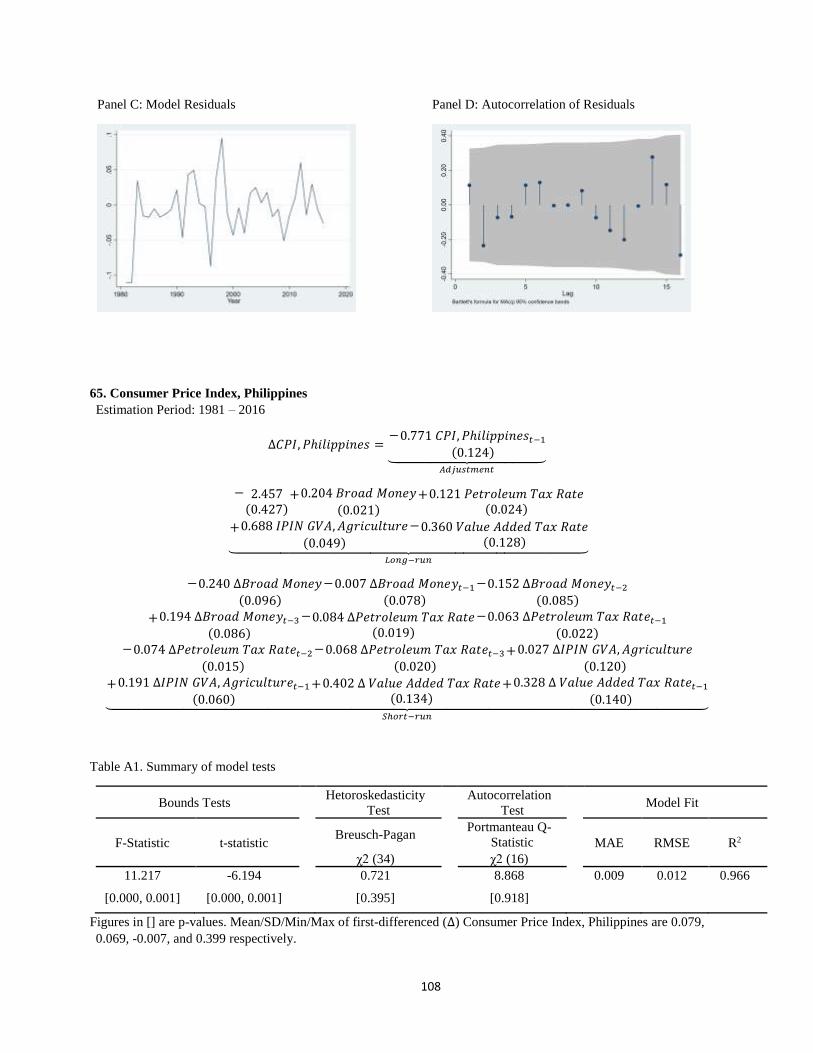
108
Panel C: Model Residuals Panel D: Autocorrelation of Residuals
65. Consumer Price Index, Philippines
Estimation Period: 1981 – 2016
∆𝐶𝑃𝐼, 𝑃ℎ𝑖𝑙𝑖𝑝𝑝𝑖𝑛𝑒𝑠 =−0.771 𝐶𝑃𝐼, 𝑃ℎ𝑖𝑙𝑖𝑝𝑝𝑖𝑛𝑒𝑠𝑡−1
(0.124)⏟ 𝐴𝑑𝑗𝑢𝑠𝑡𝑚𝑒𝑛𝑡
− 2.457(0.427)
+0.204 𝐵𝑟𝑜𝑎𝑑 𝑀𝑜𝑛𝑒𝑦
(0.021)+0.121 𝑃𝑒𝑡𝑟𝑜𝑙𝑒𝑢𝑚 𝑇𝑎𝑥 𝑅𝑎𝑡𝑒
(0.024)
+0.688 𝐼𝑃𝐼𝑁 𝐺𝑉𝐴, 𝐴𝑔𝑟𝑖𝑐𝑢𝑙𝑡𝑢𝑟𝑒
(0.049)
−0.360 𝑉𝑎𝑙𝑢𝑒 𝐴𝑑𝑑𝑒𝑑 𝑇𝑎𝑥 𝑅𝑎𝑡𝑒(0.128)⏟
𝐿𝑜𝑛𝑔−𝑟𝑢𝑛
−0.240 ∆𝐵𝑟𝑜𝑎𝑑 𝑀𝑜𝑛𝑒𝑦(0.096)
−0.007 ∆𝐵𝑟𝑜𝑎𝑑 𝑀𝑜𝑛𝑒𝑦𝑡−1(0.078)
−0.152 ∆𝐵𝑟𝑜𝑎𝑑 𝑀𝑜𝑛𝑒𝑦𝑡−2(0.085)
+0.194 ∆𝐵𝑟𝑜𝑎𝑑 𝑀𝑜𝑛𝑒𝑦𝑡−3(0.086)
−0.084 ∆𝑃𝑒𝑡𝑟𝑜𝑙𝑒𝑢𝑚 𝑇𝑎𝑥 𝑅𝑎𝑡𝑒(0.019)
−0.063 ∆𝑃𝑒𝑡𝑟𝑜𝑙𝑒𝑢𝑚 𝑇𝑎𝑥 𝑅𝑎𝑡𝑒𝑡−1(0.022)
−0.074 ∆𝑃𝑒𝑡𝑟𝑜𝑙𝑒𝑢𝑚 𝑇𝑎𝑥 𝑅𝑎𝑡𝑒𝑡−2(0.015)
−0.068 ∆𝑃𝑒𝑡𝑟𝑜𝑙𝑒𝑢𝑚 𝑇𝑎𝑥 𝑅𝑎𝑡𝑒𝑡−3(0.020)
+0.027 ∆𝐼𝑃𝐼𝑁 𝐺𝑉𝐴, 𝐴𝑔𝑟𝑖𝑐𝑢𝑙𝑡𝑢𝑟𝑒
(0.120)
+0.191 ∆𝐼𝑃𝐼𝑁 𝐺𝑉𝐴, 𝐴𝑔𝑟𝑖𝑐𝑢𝑙𝑡𝑢𝑟𝑒𝑡−1(0.060)
+0.402 ∆ 𝑉𝑎𝑙𝑢𝑒 𝐴𝑑𝑑𝑒𝑑 𝑇𝑎𝑥 𝑅𝑎𝑡𝑒(0.134)
+0.328 ∆ 𝑉𝑎𝑙𝑢𝑒 𝐴𝑑𝑑𝑒𝑑 𝑇𝑎𝑥 𝑅𝑎𝑡𝑒𝑡−1(0.140)⏟
𝑆ℎ𝑜𝑟𝑡−𝑟𝑢𝑛
Table A1. Summary of model tests
Bounds Tests Hetoroskedasticity
Test Autocorrelation
Test Model Fit
F-Statistic t-statistic Breusch-Pagan Portmanteau Q-
Statistic MAE RMSE R2
χ2 (34) χ2 (16)
11.217 -6.194 0.721 8.868 0.009 0.012 0.966
[0.000, 0.001] [0.000, 0.001] [0.395] [0.918]
Figures in [] are p-values. Mean/SD/Min/Max of first-differenced (∆) Consumer Price Index, Philippines are 0.079,
0.069, -0.007, and 0.399 respectively.
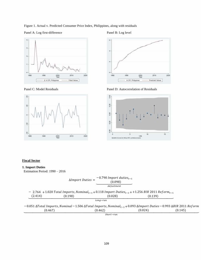
109
Figure 1. Actual v. Predicted Consumer Price Index, Philippines, along with residuals
Panel A: Log first-difference Panel B: Log level
Panel C: Model Residuals Panel D: Autocorrelation of Residuals
Fiscal Sector
1. Import Duties
Estimation Period: 1990 – 2016
∆𝐼𝑚𝑝𝑜𝑟𝑡 𝐷𝑢𝑡𝑖𝑒𝑠 =−0.790 𝐼𝑚𝑝𝑜𝑟𝑡 𝑑𝑢𝑡𝑖𝑒𝑠𝑡−1
(0.098)⏟ 𝐴𝑑𝑗𝑢𝑠𝑡𝑚𝑒𝑛𝑡
− 2.764(2.414)
+1.020 𝑇𝑜𝑡𝑎𝑙 𝐼𝑚𝑝𝑜𝑟𝑡𝑠, 𝑁𝑜𝑚𝑖𝑛𝑎𝑙𝑡−1(0.198)
+0.118 𝐼𝑚𝑝𝑜𝑟𝑡 𝐷𝑢𝑡𝑖𝑒𝑠𝑡−1(0.028)
++1.256 𝐵𝐼𝑅 2011 𝑅𝑒𝑓𝑜𝑟𝑚𝑡−1
(0.139)⏟ 𝐿𝑜𝑛𝑔−𝑟𝑢𝑛
−0.051 ∆𝑇𝑜𝑡𝑎𝑙 𝐼𝑚𝑝𝑜𝑟𝑡𝑠, 𝑁𝑜𝑚𝑖𝑛𝑎𝑙(0.467)
−1.506 ∆𝑇𝑜𝑡𝑎𝑙 𝐼𝑚𝑝𝑜𝑟𝑡𝑠, 𝑁𝑜𝑚𝑖𝑛𝑎𝑙𝑡−1(0.462)
+0.093 ∆𝐼𝑚𝑝𝑜𝑟𝑡 𝐷𝑢𝑡𝑖𝑒𝑠(0.024)
−0.993 ∆𝐵𝐼𝑅 2011 𝑅𝑒𝑓𝑜𝑟𝑚
(0.145)⏟ 𝑆ℎ𝑜𝑟𝑡−𝑟𝑢𝑛
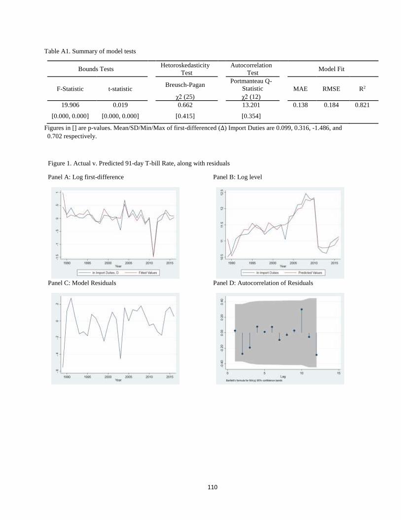
110
Table A1. Summary of model tests
Bounds Tests Hetoroskedasticity
Test Autocorrelation
Test Model Fit
F-Statistic t-statistic Breusch-Pagan Portmanteau Q-
Statistic MAE RMSE R2
χ2 (25) χ2 (12)
19.906 0.019 0.662 13.201 0.138 0.184 0.821
[0.000, 0.000] [0.000, 0.000] [0.415] [0.354]
Figures in [] are p-values. Mean/SD/Min/Max of first-differenced (∆) Import Duties are 0.099, 0.316, -1.486, and
0.702 respectively.
Figure 1. Actual v. Predicted 91-day T-bill Rate, along with residuals
Panel A: Log first-difference Panel B: Log level
Panel C: Model Residuals Panel D: Autocorrelation of Residuals

111
2. Excise Tax on Imports
Estimation Period: 1990 – 2016
∆𝐼𝑚𝑝𝑜𝑟𝑡 𝐷𝑢𝑡𝑖𝑒𝑠 𝑎𝑛𝑑 𝐸𝑥𝑐𝑖𝑠𝑒 𝑇𝑎𝑥𝑒𝑠 =−0.873 𝐼𝑚𝑝𝑜𝑟𝑡 𝐷𝑢𝑡𝑖𝑒𝑠 𝑎𝑛𝑑 𝐸𝑥𝑐𝑖𝑠𝑒 𝑇𝑎𝑥𝑒𝑠𝑡−1
(0.101)⏟ 𝐴𝑑𝑗𝑢𝑠𝑡𝑚𝑒𝑛𝑡
− 3.338(2.125)
+1.042 𝑇𝑜𝑡𝑎𝑙 𝐼𝑚𝑝𝑜𝑟𝑡𝑠, 𝑁𝑜𝑚𝑖𝑛𝑎𝑙𝑡−1(0.155)
+0.119 𝐼𝑚𝑝𝑜𝑟𝑡 𝑑𝑢𝑡𝑖𝑒𝑠𝑡−1(0.022)
−0.916 𝐵𝐼𝑅 2011 𝑅𝑒𝑓𝑜𝑟𝑚 𝑡−1(0.111)⏟
𝐿𝑜𝑛𝑔−𝑟𝑢𝑛
+0.174 ∆𝐼𝑚𝑝𝑜𝑟𝑡 𝐷𝑢𝑡𝑖𝑒𝑠 𝑎𝑛𝑑 𝐸𝑥𝑐𝑖𝑠𝑒 𝑇𝑎𝑥𝑒𝑠𝑡−1(0.097)
+0.060 ∆𝑇𝑜𝑡𝑎𝑙 𝐼𝑚𝑝𝑜𝑟𝑡𝑠, 𝑁𝑜𝑚𝑖𝑛𝑎𝑙
(0.403)
−1.599 ∆𝑇𝑜𝑡𝑎𝑙 𝐼𝑚𝑝𝑜𝑟𝑡𝑠,𝑁𝑜𝑚𝑖𝑛𝑎𝑙𝑡−1(0.404)
+0.104 ∆𝐼𝑚𝑝𝑜𝑟𝑡 𝐷𝑢𝑡𝑖𝑒𝑠(0.022)
−0.800 𝐵𝐼𝑅 2011 𝑅𝑒𝑓𝑜𝑟𝑚
(0.122)⏟ 𝑆ℎ𝑜𝑟𝑡−𝑟𝑢𝑛
Table A1. Summary of model tests
Bounds Tests Hetoroskedasticity
Test Autocorrelation
Test Model Fit
F-Statistic t-statistic Breusch-Pagan Portmanteau Q-
Statistic MAE RMSE R2
χ2 (25) χ2 (12)
8.000 -4.750 0.079 3.516 0.505 0.723 0.510
[0.003, 0.010] [0.001, 0.006] [0.777] [0.990]
Figures in [] are p-values. Mean/SD/Min/Max of first-differenced (∆) Excise Tax on Imports are 0.089, 1.361, -4.770,
and 4.770 respectively.
Figure 1. Actual v. Predicted Excise Tax on Imports, along with residuals
Panel A: Log first-difference Panel B: Log level
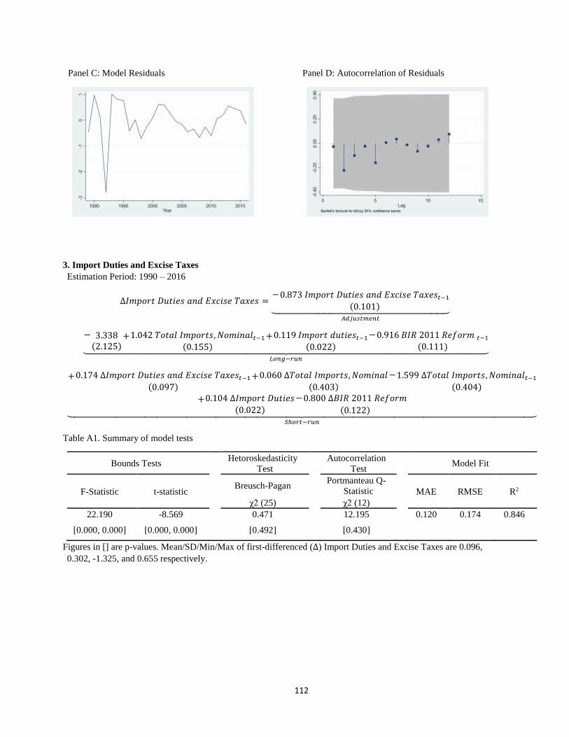
112
Panel C: Model Residuals Panel D: Autocorrelation of Residuals
3. Import Duties and Excise Taxes
Estimation Period: 1990 – 2016
∆𝐼𝑚𝑝𝑜𝑟𝑡 𝐷𝑢𝑡𝑖𝑒𝑠 𝑎𝑛𝑑 𝐸𝑥𝑐𝑖𝑠𝑒 𝑇𝑎𝑥𝑒𝑠 =−0.873 𝐼𝑚𝑝𝑜𝑟𝑡 𝐷𝑢𝑡𝑖𝑒𝑠 𝑎𝑛𝑑 𝐸𝑥𝑐𝑖𝑠𝑒 𝑇𝑎𝑥𝑒𝑠𝑡−1
(0.101)⏟ 𝐴𝑑𝑗𝑢𝑠𝑡𝑚𝑒𝑛𝑡
− 3.338(2.125)
+1.042 𝑇𝑜𝑡𝑎𝑙 𝐼𝑚𝑝𝑜𝑟𝑡𝑠, 𝑁𝑜𝑚𝑖𝑛𝑎𝑙𝑡−1(0.155)
+0.119 𝐼𝑚𝑝𝑜𝑟𝑡 𝑑𝑢𝑡𝑖𝑒𝑠𝑡−1(0.022)
−0.916 𝐵𝐼𝑅 2011 𝑅𝑒𝑓𝑜𝑟𝑚 𝑡−1(0.111)⏟
𝐿𝑜𝑛𝑔−𝑟𝑢𝑛
+0.174 ∆𝐼𝑚𝑝𝑜𝑟𝑡 𝐷𝑢𝑡𝑖𝑒𝑠 𝑎𝑛𝑑 𝐸𝑥𝑐𝑖𝑠𝑒 𝑇𝑎𝑥𝑒𝑠𝑡−1(0.097)
+0.060 ∆𝑇𝑜𝑡𝑎𝑙 𝐼𝑚𝑝𝑜𝑟𝑡𝑠, 𝑁𝑜𝑚𝑖𝑛𝑎𝑙
(0.403)
−1.599 ∆𝑇𝑜𝑡𝑎𝑙 𝐼𝑚𝑝𝑜𝑟𝑡𝑠,𝑁𝑜𝑚𝑖𝑛𝑎𝑙𝑡−1(0.404)
+0.104 ∆𝐼𝑚𝑝𝑜𝑟𝑡 𝐷𝑢𝑡𝑖𝑒𝑠(0.022)
−0.800 ∆𝐵𝐼𝑅 2011 𝑅𝑒𝑓𝑜𝑟𝑚
(0.122)⏟ 𝑆ℎ𝑜𝑟𝑡−𝑟𝑢𝑛
Table A1. Summary of model tests
Bounds Tests Hetoroskedasticity
Test Autocorrelation
Test Model Fit
F-Statistic t-statistic Breusch-Pagan Portmanteau Q-
Statistic MAE RMSE R2
χ2 (25) χ2 (12)
22.190 -8.569 0.471 12.195 0.120 0.174 0.846
[0.000, 0.000] [0.000, 0.000] [0.492] [0.430]
Figures in [] are p-values. Mean/SD/Min/Max of first-differenced (∆) Import Duties and Excise Taxes are 0.096,
0.302, -1.325, and 0.655 respectively.
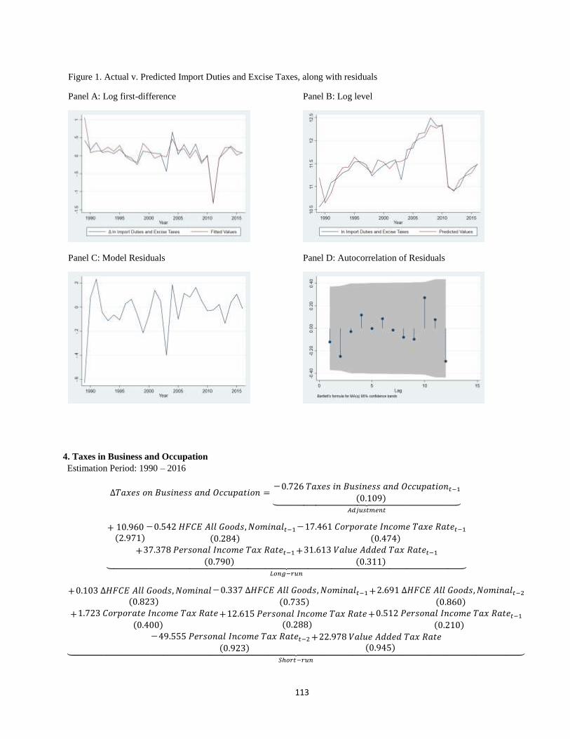
113
4. Taxes in Business and Occupation
Estimation Period: 1990 – 2016
∆𝑇𝑎𝑥𝑒𝑠 𝑜𝑛 𝐵𝑢𝑠𝑖𝑛𝑒𝑠𝑠 𝑎𝑛𝑑 𝑂𝑐𝑐𝑢𝑝𝑎𝑡𝑖𝑜𝑛 =−0.726 𝑇𝑎𝑥𝑒𝑠 𝑖𝑛 𝐵𝑢𝑠𝑖𝑛𝑒𝑠𝑠 𝑎𝑛𝑑 𝑂𝑐𝑐𝑢𝑝𝑎𝑡𝑖𝑜𝑛𝑡−1
(0.109)⏟ 𝐴𝑑𝑗𝑢𝑠𝑡𝑚𝑒𝑛𝑡
+ 10.960(2.971)
−0.542 𝐻𝐹𝐶𝐸 𝐴𝑙𝑙 𝐺𝑜𝑜𝑑𝑠, 𝑁𝑜𝑚𝑖𝑛𝑎𝑙𝑡−1(0.284)
−17.461 𝐶𝑜𝑟𝑝𝑜𝑟𝑎𝑡𝑒 𝐼𝑛𝑐𝑜𝑚𝑒 𝑇𝑎𝑥𝑒 𝑅𝑎𝑡𝑒𝑡−1(0.474)
+37.378 𝑃𝑒𝑟𝑠𝑜𝑛𝑎𝑙 𝐼𝑛𝑐𝑜𝑚𝑒 𝑇𝑎𝑥 𝑅𝑎𝑡𝑒𝑡−1(0.790)
+31.613 𝑉𝑎𝑙𝑢𝑒 𝐴𝑑𝑑𝑒𝑑 𝑇𝑎𝑥 𝑅𝑎𝑡𝑒𝑡−1(0.311)⏟
𝐿𝑜𝑛𝑔−𝑟𝑢𝑛
+0.103 ∆𝐻𝐹𝐶𝐸 𝐴𝑙𝑙 𝐺𝑜𝑜𝑑𝑠, 𝑁𝑜𝑚𝑖𝑛𝑎𝑙(0.823)
−0.337 ∆𝐻𝐹𝐶𝐸 𝐴𝑙𝑙 𝐺𝑜𝑜𝑑𝑠, 𝑁𝑜𝑚𝑖𝑛𝑎𝑙𝑡−1(0.735)
+2.691 ∆𝐻𝐹𝐶𝐸 𝐴𝑙𝑙 𝐺𝑜𝑜𝑑𝑠, 𝑁𝑜𝑚𝑖𝑛𝑎𝑙𝑡−2(0.860)
+1.723 𝐶𝑜𝑟𝑝𝑜𝑟𝑎𝑡𝑒 𝐼𝑛𝑐𝑜𝑚𝑒 𝑇𝑎𝑥 𝑅𝑎𝑡𝑒(0.400)
+12.615 𝑃𝑒𝑟𝑠𝑜𝑛𝑎𝑙 𝐼𝑛𝑐𝑜𝑚𝑒 𝑇𝑎𝑥 𝑅𝑎𝑡𝑒(0.288)
+0.512 𝑃𝑒𝑟𝑠𝑜𝑛𝑎𝑙 𝐼𝑛𝑐𝑜𝑚𝑒 𝑇𝑎𝑥 𝑅𝑎𝑡𝑒𝑡−1(0.210)
−49.555 𝑃𝑒𝑟𝑠𝑜𝑛𝑎𝑙 𝐼𝑛𝑐𝑜𝑚𝑒 𝑇𝑎𝑥 𝑅𝑎𝑡𝑒𝑡−2(0.923)
+22.978 𝑉𝑎𝑙𝑢𝑒 𝐴𝑑𝑑𝑒𝑑 𝑇𝑎𝑥 𝑅𝑎𝑡𝑒(0.945)⏟
𝑆ℎ𝑜𝑟𝑡−𝑟𝑢𝑛
Figure 1. Actual v. Predicted Import Duties and Excise Taxes, along with residuals
Panel A: Log first-difference Panel B: Log level
Panel C: Model Residuals Panel D: Autocorrelation of Residuals

114
Table A1. Summary of model tests
Bounds Tests Hetoroskedasticity
Test Autocorrelation
Test Model Fit
F-Statistic t-statistic Breusch-Pagan Portmanteau Q-
Statistic MAE RMSE R2
χ2 (35) χ2 (16)
11.159 -6.624 0.902 12.417 0.147 0.191 0.755
[0.000, 0.000] [0.000, 0.000] [0.342] [0.714]
Figures in [] are p-values. Mean/SD/Min/Max of first-differenced (∆)Taxes in Business and Occupation are 0.151,
0.351, -0.530, and 1.356 respectively.
Figure 1. Actual v. Predicted Taxes in Business and Occupation, along with residuals
Panel A: Log first-difference Panel B: Log level
Panel C: Model Residuals Panel D: Autocorrelation of Residuals

115
5. Other Indirect Taxes
Estimation Period: 1979 – 2016
∆𝑂𝑡ℎ𝑒𝑟 𝐼𝑛𝑑𝑖𝑟𝑒𝑐𝑡 𝑇𝑎𝑥𝑒𝑠 =−0.493 𝑂𝑡ℎ𝑒𝑟 𝐼𝑛𝑑𝑖𝑟𝑒𝑐𝑡 𝑇𝑎𝑥𝑒𝑠𝑡−1
(0.113)⏟ 𝐴𝑑𝑗𝑢𝑠𝑡𝑚𝑒𝑛𝑡
− 3.009(0.878)
+1.078 𝐻𝐹𝐶𝐸 𝐴𝑙𝑙 𝐺𝑜𝑜𝑑𝑠, 𝑁𝑜𝑚𝑖𝑛𝑎𝑙𝑡−1(0.116)
+7.671 𝑉𝑎𝑙𝑢𝑒 𝐴𝑑𝑑𝑒𝑑 𝑇𝑎𝑥 𝑅𝑎𝑡𝑒𝑡−1(0.956)⏟
𝐿𝑜𝑛𝑔−𝑟𝑢𝑛
+0.325 ∆𝑂𝑡ℎ𝑒𝑟 𝐼𝑛𝑑𝑖𝑟𝑒𝑐𝑡 𝑇𝑎𝑥𝑒𝑠𝑡−1(0.134)
+0.513 ∆𝐻𝐹𝐶𝐸 𝐴𝑙𝑙 𝐺𝑜𝑜𝑑𝑠, 𝑁𝑜𝑚𝑖𝑛𝑎𝑙(0.117)
+3.782 ∆𝑉𝑎𝑙𝑢𝑒 𝐴𝑑𝑑𝑒𝑑 𝑇𝑎𝑥 𝑅𝑎𝑡𝑒(0.121)⏟
𝑆ℎ𝑜𝑟𝑡−𝑟𝑢𝑛
Table A1. Summary of model tests
Bounds Tests Hetoroskedasticity
Test Autocorrelation
Test Model Fit
F-Statistic t-statistic Breusch-Pagan Portmanteau Q-
Statistic MAE RMSE R2
χ2 (36) χ2 (17)
7.014 -4.346 0.035 23.379 0.220 0.330 0.397
[0.004, 0.013] [0.001, 0.010] [0.851] [0.137]
Figures in [] are p-values. Mean/SD/Min/Max of first-differenced (∆) Other Indirect Taxes are 0.130, 0.351, -0.785,
and 1.028 respectively.
Figure 1. Actual v. Predicted Other Indirect Taxes, along with residuals
Panel A: Log first-difference Panel B: Log level
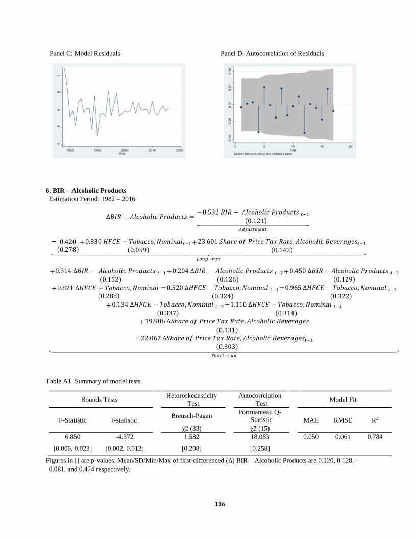
116
Panel C: Model Residuals Panel D: Autocorrelation of Residuals
6. BIR – Alcoholic Products
Estimation Period: 1982 – 2016
∆𝐵𝐼𝑅 − 𝐴𝑙𝑐𝑜ℎ𝑜𝑙𝑖𝑐 𝑃𝑟𝑜𝑑𝑢𝑐𝑡𝑠 =−0.532 𝐵𝐼𝑅 − 𝐴𝑙𝑐𝑜ℎ𝑜𝑙𝑖𝑐 𝑃𝑟𝑜𝑑𝑢𝑐𝑡𝑠 𝑡−1
(0.121)⏟ 𝐴𝑑𝑗𝑢𝑠𝑡𝑚𝑒𝑛𝑡
− 0.420(0.278)
+0.830 𝐻𝐹𝐶𝐸 − 𝑇𝑜𝑏𝑎𝑐𝑐𝑜, 𝑁𝑜𝑚𝑖𝑛𝑎𝑙𝑡−1(0.059)
+23.601 𝑆ℎ𝑎𝑟𝑒 𝑜𝑓 𝑃𝑟𝑖𝑐𝑒 𝑇𝑎𝑥 𝑅𝑎𝑡𝑒, 𝐴𝑙𝑐𝑜ℎ𝑜𝑙𝑖𝑐 𝐵𝑒𝑣𝑒𝑟𝑎𝑔𝑒𝑠𝑡−1(0.142)⏟
𝐿𝑜𝑛𝑔−𝑟𝑢𝑛
+0.314 ∆𝐵𝐼𝑅 − 𝐴𝑙𝑐𝑜ℎ𝑜𝑙𝑖𝑐 𝑃𝑟𝑜𝑑𝑢𝑐𝑡𝑠 𝑡−1(0.152)
+0.204 ∆𝐵𝐼𝑅 − 𝐴𝑙𝑐𝑜ℎ𝑜𝑙𝑖𝑐 𝑃𝑟𝑜𝑑𝑢𝑐𝑡𝑠 𝑡−2(0.126)
+0.450 ∆𝐵𝐼𝑅 − 𝐴𝑙𝑐𝑜ℎ𝑜𝑙𝑖𝑐 𝑃𝑟𝑜𝑑𝑢𝑐𝑡𝑠 𝑡−3(0.129)
+0.821 ∆𝐻𝐹𝐶𝐸 − 𝑇𝑜𝑏𝑎𝑐𝑐𝑜, 𝑁𝑜𝑚𝑖𝑛𝑎𝑙 (0.288)
−0.520 ∆𝐻𝐹𝐶𝐸 − 𝑇𝑜𝑏𝑎𝑐𝑐𝑜, 𝑁𝑜𝑚𝑖𝑛𝑎𝑙 𝑡−1(0.324)
−0.965 ∆𝐻𝐹𝐶𝐸 − 𝑇𝑜𝑏𝑎𝑐𝑐𝑜, 𝑁𝑜𝑚𝑖𝑛𝑎𝑙 𝑡−2(0.322)
+0.134 ∆𝐻𝐹𝐶𝐸 − 𝑇𝑜𝑏𝑎𝑐𝑐𝑜, 𝑁𝑜𝑚𝑖𝑛𝑎𝑙 𝑡−3(0.337)
−1.110 ∆𝐻𝐹𝐶𝐸 − 𝑇𝑜𝑏𝑎𝑐𝑐𝑜, 𝑁𝑜𝑚𝑖𝑛𝑎𝑙 𝑡−4(0.314)
+19.906 ∆𝑆ℎ𝑎𝑟𝑒 𝑜𝑓 𝑃𝑟𝑖𝑐𝑒 𝑇𝑎𝑥 𝑅𝑎𝑡𝑒, 𝐴𝑙𝑐𝑜ℎ𝑜𝑙𝑖𝑐 𝐵𝑒𝑣𝑒𝑟𝑎𝑔𝑒𝑠
(0.131)−22.067 ∆𝑆ℎ𝑎𝑟𝑒 𝑜𝑓 𝑃𝑟𝑖𝑐𝑒 𝑇𝑎𝑥 𝑅𝑎𝑡𝑒, 𝐴𝑙𝑐𝑜ℎ𝑜𝑙𝑖𝑐 𝐵𝑒𝑣𝑒𝑟𝑎𝑔𝑒𝑠𝑡−1
(0.303)⏟ 𝑆ℎ𝑜𝑟𝑡−𝑟𝑢𝑛
Table A1. Summary of model tests
Bounds Tests Hetoroskedasticity
Test Autocorrelation
Test Model Fit
F-Statistic t-statistic Breusch-Pagan Portmanteau Q-
Statistic MAE RMSE R2
χ2 (33) χ2 (15)
6.850 -4.372 1.582 18.083 0.050 0.061 0.784
[0.006, 0.023] [0.002, 0.012] [0.208] [0.258]
Figures in [] are p-values. Mean/SD/Min/Max of first-differenced (∆) BIR – Alcoholic Products are 0.120, 0.128, -
0.081, and 0.474 respectively.

117
Figure 1. Actual v. Predicted BIR – Alcoholic Products, along with residuals
Panel A: Log first-difference Panel B: Log level
Panel C: Model Residuals
Panel D: Autocorrelation of Residuals
7. BIR – Tobacco Products
Estimation Period: 1979 – 2016
∆𝐵𝐼𝑅 − 𝑇𝑜𝑏𝑎𝑐𝑐𝑜 𝑃𝑟𝑜𝑑𝑢𝑐𝑡𝑠 =−0.717 𝐵𝐼𝑅 − 𝑇𝑜𝑏𝑎𝑐𝑐𝑜 𝑃𝑟𝑜𝑑𝑢𝑐𝑡𝑠 𝑡−1
(0.139)⏟ 𝐴𝑑𝑗𝑢𝑠𝑡𝑚𝑒𝑛𝑡
− 0.282(0.287)
+0.949 𝐻𝐹𝐶𝐸 − 𝐴𝑙𝑐𝑜ℎ𝑜𝑙, 𝑁𝑜𝑚𝑖𝑛𝑎𝑙𝑡−1(0.037)
−1.016 𝑆ℎ𝑎𝑟𝑒 𝑜𝑓 𝑃𝑟𝑖𝑐𝑒 𝑇𝑎𝑥 𝑅𝑎𝑡𝑒, 𝑇𝑜𝑏𝑎𝑐𝑐𝑜𝑡−1(0.971)⏟
𝐿𝑜𝑛𝑔−𝑟𝑢𝑛
−0.219 ∆𝐻𝐹𝐶𝐸 − 𝐴𝑙𝑐𝑜ℎ𝑜𝑙, 𝑁𝑜𝑚𝑖𝑛𝑎𝑙 (0.306)
−0.641 ∆𝐻𝐹𝐶𝐸 − 𝐴𝑙𝑐𝑜ℎ𝑜𝑙, 𝑁𝑜𝑚𝑖𝑛𝑎𝑙 𝑡−1(0.321)
+7.039 ∆𝑆ℎ𝑎𝑟𝑒 𝑜𝑓 𝑃𝑟𝑖𝑐𝑒 𝑇𝑎𝑥 𝑅𝑎𝑡𝑒, 𝑇𝑜𝑏𝑎𝑐𝑐𝑜
(0.063)⏟ 𝑆ℎ𝑜𝑟𝑡−𝑟𝑢𝑛
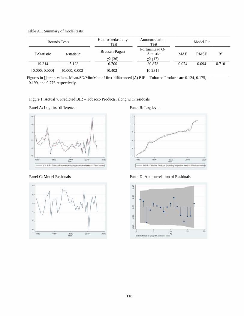
118
Table A1. Summary of model tests
Bounds Tests Hetoroskedasticity
Test Autocorrelation
Test Model Fit
F-Statistic t-statistic Breusch-Pagan Portmanteau Q-
Statistic MAE RMSE R2
χ2 (36) χ2 (17)
19.214 -5.123 0.700 20.873 0.074 0.094 0.710
[0.000, 0.000] [0.000, 0.002] [0.402] [0.231]
Figures in [] are p-values. Mean/SD/Min/Max of first-differenced (∆) BIR – Tobacco Products are 0.124, 0.175, -
0.199, and 0.776 respectively.
Figure 1. Actual v. Predicted BIR – Tobacco Products, along with residuals
Panel A: Log first-difference Panel B: Log level
Panel C: Model Residuals Panel D: Autocorrelation of Residuals
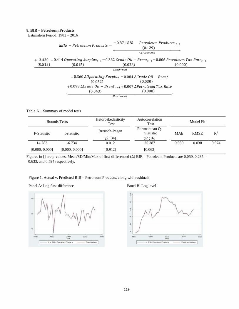
119
8. BIR – Petroleum Products
Estimation Period: 1981 – 2016
∆𝐵𝐼𝑅 − 𝑃𝑒𝑡𝑟𝑜𝑙𝑒𝑢𝑚 𝑃𝑟𝑜𝑑𝑢𝑐𝑡𝑠 =−0.871 𝐵𝐼𝑅 − 𝑃𝑒𝑡𝑟𝑜𝑙𝑒𝑢𝑚 𝑃𝑟𝑜𝑑𝑢𝑐𝑡𝑠 𝑡−1
(0.129)⏟ 𝐴𝑑𝑗𝑢𝑠𝑡𝑚𝑒𝑛𝑡
+ 3.430(0.515)
+0.414 𝑂𝑝𝑒𝑟𝑎𝑡𝑖𝑛𝑔 𝑆𝑢𝑟𝑝𝑙𝑢𝑠𝑡−1(0.015)
−0.382 𝐶𝑟𝑢𝑑𝑒 𝑂𝑖𝑙 − 𝐵𝑟𝑒𝑛𝑡𝑡−1(0.028)
−0.006 𝑃𝑒𝑡𝑟𝑜𝑙𝑒𝑢𝑚 𝑇𝑎𝑥 𝑅𝑎𝑡𝑒𝑡−1(0.000)⏟
𝐿𝑜𝑛𝑔−𝑟𝑢𝑛
+0.360 ∆𝑂𝑝𝑒𝑟𝑎𝑡𝑖𝑛𝑔 𝑆𝑢𝑟𝑝𝑙𝑢𝑠
(0.052)
−0.084 ∆𝐶𝑟𝑢𝑑𝑒 𝑂𝑖𝑙 − 𝐵𝑟𝑒𝑛𝑡 (0.030)
+0.098 ∆𝐶𝑟𝑢𝑑𝑒 𝑂𝑖𝑙 − 𝐵𝑟𝑒𝑛𝑡 𝑡−1(0.043)
+0.007 ∆𝑃𝑒𝑡𝑟𝑜𝑙𝑒𝑢𝑚 𝑇𝑎𝑥 𝑅𝑎𝑡𝑒 (0.000)⏟
𝑆ℎ𝑜𝑟𝑡−𝑟𝑢𝑛
Table A1. Summary of model tests
Bounds Tests Hetoroskedasticity
Test Autocorrelation
Test Model Fit
F-Statistic t-statistic Breusch-Pagan Portmanteau Q-
Statistic MAE RMSE R2
χ2 (34) χ2 (16)
14.283 -6.734 0.012 25.387 0.030 0.038 0.974
[0.000, 0.000] [0.000, 0.000] [0.912] [0.063]
Figures in [] are p-values. Mean/SD/Min/Max of first-differenced (∆) BIR – Petroleum Products are 0.050, 0.235, -
0.633, and 0.594 respectively.
Figure 1. Actual v. Predicted BIR – Petroleum Products, along with residuals
Panel A: Log first-difference Panel B: Log level
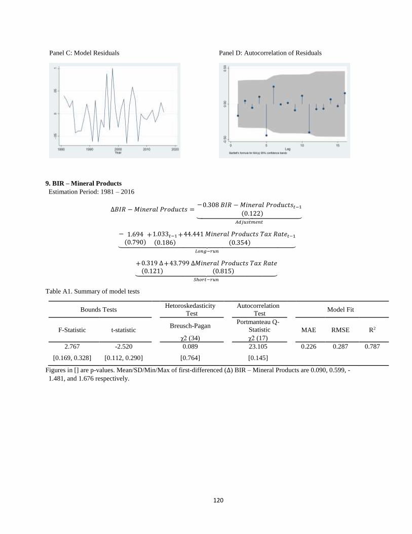
120
Panel C: Model Residuals Panel D: Autocorrelation of Residuals
9. BIR – Mineral Products
Estimation Period: 1981 – 2016
∆𝐵𝐼𝑅 − 𝑀𝑖𝑛𝑒𝑟𝑎𝑙 𝑃𝑟𝑜𝑑𝑢𝑐𝑡𝑠 =−0.308 𝐵𝐼𝑅 − 𝑀𝑖𝑛𝑒𝑟𝑎𝑙 𝑃𝑟𝑜𝑑𝑢𝑐𝑡𝑠𝑡−1
(0.122)⏟ 𝐴𝑑𝑗𝑢𝑠𝑡𝑚𝑒𝑛𝑡
− 1.694(0.790)
+1.033𝑡−1(0.186)
+44.441 𝑀𝑖𝑛𝑒𝑟𝑎𝑙 𝑃𝑟𝑜𝑑𝑢𝑐𝑡𝑠 𝑇𝑎𝑥 𝑅𝑎𝑡𝑒𝑡−1(0.354)⏟
𝐿𝑜𝑛𝑔−𝑟𝑢𝑛
+0.319 ∆(0.121)
+43.799 ∆𝑀𝑖𝑛𝑒𝑟𝑎𝑙 𝑃𝑟𝑜𝑑𝑢𝑐𝑡𝑠 𝑇𝑎𝑥 𝑅𝑎𝑡𝑒(0.815)⏟
𝑆ℎ𝑜𝑟𝑡−𝑟𝑢𝑛
Table A1. Summary of model tests
Bounds Tests Hetoroskedasticity
Test Autocorrelation
Test Model Fit
F-Statistic t-statistic Breusch-Pagan Portmanteau Q-
Statistic MAE RMSE R2
χ2 (34) χ2 (17)
2.767 -2.520 0.089 23.105 0.226 0.287 0.787
[0.169, 0.328] [0.112, 0.290] [0.764] [0.145]
Figures in [] are p-values. Mean/SD/Min/Max of first-differenced (∆) BIR – Mineral Products are 0.090, 0.599, -
1.481, and 1.676 respectively.
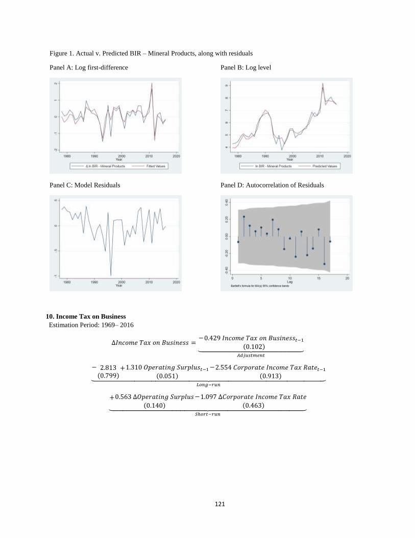
121
Figure 1. Actual v. Predicted BIR – Mineral Products, along with residuals
Panel A: Log first-difference Panel B: Log level
Panel C: Model Residuals Panel D: Autocorrelation of Residuals
10. Income Tax on Business
Estimation Period: 1969– 2016
∆𝐼𝑛𝑐𝑜𝑚𝑒 𝑇𝑎𝑥 𝑜𝑛 𝐵𝑢𝑠𝑖𝑛𝑒𝑠𝑠 =−0.429 𝐼𝑛𝑐𝑜𝑚𝑒 𝑇𝑎𝑥 𝑜𝑛 𝐵𝑢𝑠𝑖𝑛𝑒𝑠𝑠𝑡−1
(0.102)⏟ 𝐴𝑑𝑗𝑢𝑠𝑡𝑚𝑒𝑛𝑡
− 2.813(0.799)
+1.310 𝑂𝑝𝑒𝑟𝑎𝑡𝑖𝑛𝑔 𝑆𝑢𝑟𝑝𝑙𝑢𝑠𝑡−1(0.051)
−2.554 𝐶𝑜𝑟𝑝𝑜𝑟𝑎𝑡𝑒 𝐼𝑛𝑐𝑜𝑚𝑒 𝑇𝑎𝑥 𝑅𝑎𝑡𝑒𝑡−1(0.913)⏟
𝐿𝑜𝑛𝑔−𝑟𝑢𝑛
+0.563 ∆𝑂𝑝𝑒𝑟𝑎𝑡𝑖𝑛𝑔 𝑆𝑢𝑟𝑝𝑙𝑢𝑠
(0.140)
−1.097 ∆𝐶𝑜𝑟𝑝𝑜𝑟𝑎𝑡𝑒 𝐼𝑛𝑐𝑜𝑚𝑒 𝑇𝑎𝑥 𝑅𝑎𝑡𝑒(0.463)⏟
𝑆ℎ𝑜𝑟𝑡−𝑟𝑢𝑛
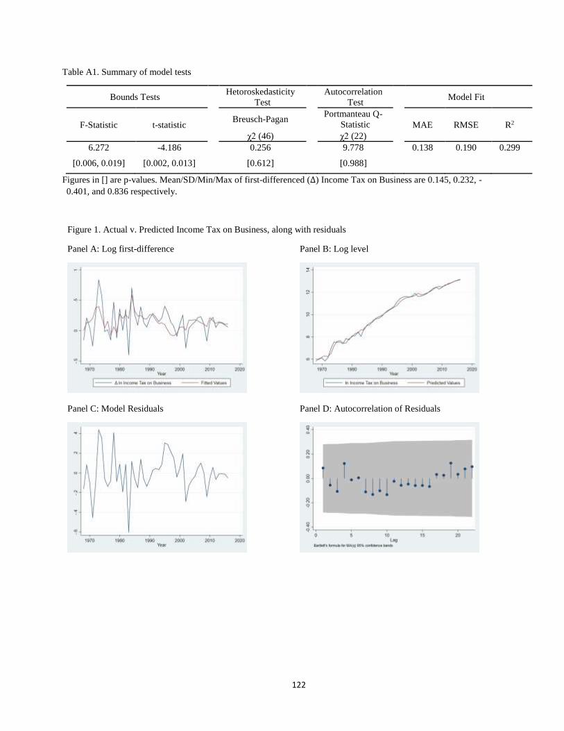
122
Table A1. Summary of model tests
Bounds Tests Hetoroskedasticity
Test Autocorrelation
Test Model Fit
F-Statistic t-statistic Breusch-Pagan Portmanteau Q-
Statistic MAE RMSE R2
χ2 (46) χ2 (22)
6.272 -4.186 0.256 9.778 0.138 0.190 0.299
[0.006, 0.019] [0.002, 0.013] [0.612] [0.988]
Figures in [] are p-values. Mean/SD/Min/Max of first-differenced (∆) Income Tax on Business are 0.145, 0.232, -
0.401, and 0.836 respectively.
Figure 1. Actual v. Predicted Income Tax on Business, along with residuals
Panel A: Log first-difference Panel B: Log level
Panel C: Model Residuals Panel D: Autocorrelation of Residuals

123
11. Income Tax on Individual
Estimation Period: 1969 – 2016
∆𝐼𝑛𝑐𝑜𝑚𝑒 𝑇𝑎𝑥 𝑜𝑛 𝐼𝑛𝑑𝑖𝑣𝑖𝑑𝑢𝑎𝑙 =−0.471 𝐼𝑛𝑐𝑜𝑚𝑒 𝑇𝑎𝑥 𝑜𝑛 𝐼𝑛𝑑𝑖𝑣𝑖𝑑𝑢𝑎𝑙𝑡−1
(0.135)⏟ 𝐴𝑑𝑗𝑢𝑠𝑡𝑚𝑒𝑛𝑡
− 0.589(1.108)
+0.758 𝐶𝑜𝑚𝑝𝑒𝑛𝑠𝑎𝑡𝑖𝑜𝑛 𝑜𝑓 𝑅𝑒𝑠𝑖𝑑𝑒𝑛𝑡𝑠𝑡−1(0.227)
+11.845 𝑃𝑒𝑟𝑠𝑜𝑛𝑎𝑙 𝐼𝑛𝑐𝑜𝑚𝑒 𝑇𝑎𝑥 𝑅𝑎𝑡𝑒𝑡−1(0.453)⏟
𝐿𝑜𝑛𝑔−𝑟𝑢𝑛
+0.358 ∆𝐶𝑜𝑚𝑝𝑒𝑛𝑠𝑎𝑡𝑖𝑜𝑛 𝑜𝑓 𝑅𝑒𝑠𝑖𝑑𝑒𝑛𝑡𝑠
(0.166)+5.591 𝑃𝑒𝑟𝑠𝑜𝑛𝑎𝑙 𝐼𝑛𝑐𝑜𝑚𝑒 𝑇𝑎𝑥 𝑅𝑎𝑡𝑒
(0.783)⏟ 𝑆ℎ𝑜𝑟𝑡−𝑟𝑢𝑛
Table A1. Summary of model tests
Bounds Tests Hetoroskedasticity
Test Autocorrelation
Test Model Fit
F-Statistic t-statistic Breusch-Pagan Portmanteau Q-
Statistic MAE RMSE R2
χ2 (46) χ2 (22)
4.900 -3.480 0.055 13.732 0.184 0.280 0.250
[0.022, 0.061] [0.012, 0.063] [0.813] [0.910]
Figures in [] are p-values. Mean/SD/Min/Max of first-differenced (∆) Income Tax on Individual are 0.148, 0.317, -
1.241, and 1.097 respectively.
Figure 1. Actual v. Predicted Income Tax on Individual, along with residuals
Panel A: Log first-difference Panel B: Log level
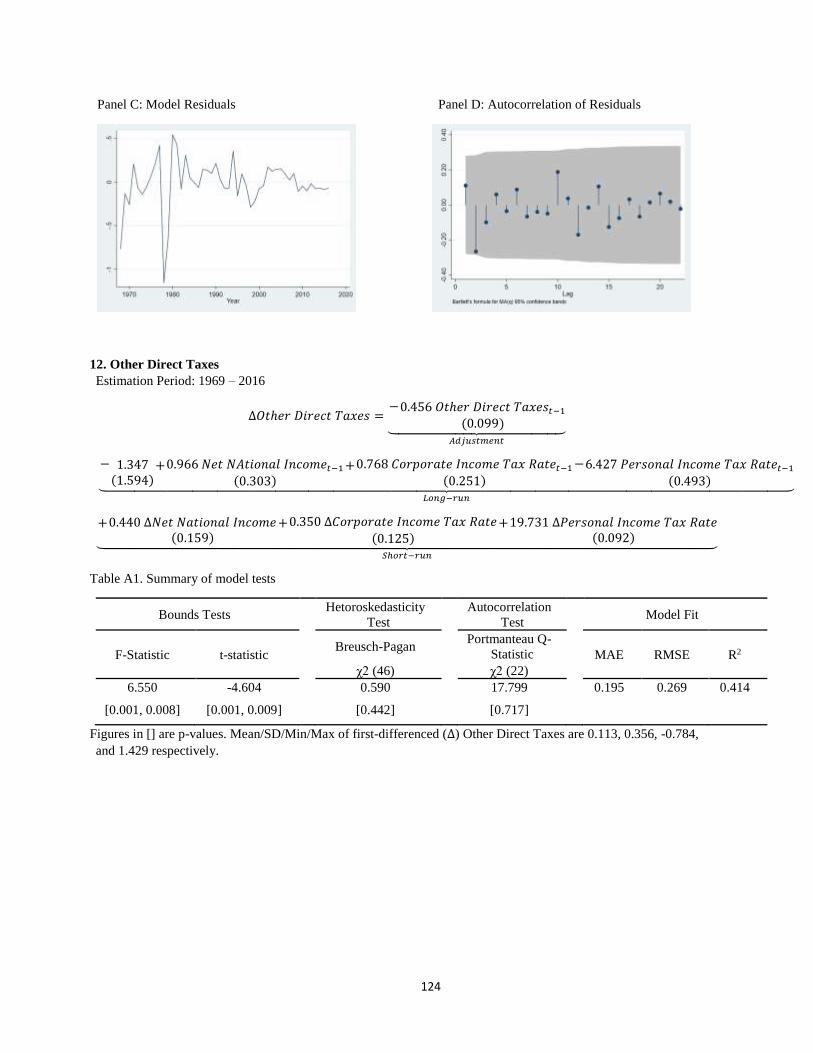
124
Panel C: Model Residuals Panel D: Autocorrelation of Residuals
12. Other Direct Taxes
Estimation Period: 1969 – 2016
∆𝑂𝑡ℎ𝑒𝑟 𝐷𝑖𝑟𝑒𝑐𝑡 𝑇𝑎𝑥𝑒𝑠 =−0.456 𝑂𝑡ℎ𝑒𝑟 𝐷𝑖𝑟𝑒𝑐𝑡 𝑇𝑎𝑥𝑒𝑠𝑡−1
(0.099)⏟ 𝐴𝑑𝑗𝑢𝑠𝑡𝑚𝑒𝑛𝑡
− 1.347(1.594)
+0.966 𝑁𝑒𝑡 𝑁𝐴𝑡𝑖𝑜𝑛𝑎𝑙 𝐼𝑛𝑐𝑜𝑚𝑒𝑡−1(0.303)
+0.768 𝐶𝑜𝑟𝑝𝑜𝑟𝑎𝑡𝑒 𝐼𝑛𝑐𝑜𝑚𝑒 𝑇𝑎𝑥 𝑅𝑎𝑡𝑒𝑡−1(0.251)
−6.427 𝑃𝑒𝑟𝑠𝑜𝑛𝑎𝑙 𝐼𝑛𝑐𝑜𝑚𝑒 𝑇𝑎𝑥 𝑅𝑎𝑡𝑒𝑡−1(0.493)⏟
𝐿𝑜𝑛𝑔−𝑟𝑢𝑛
+0.440 ∆𝑁𝑒𝑡 𝑁𝑎𝑡𝑖𝑜𝑛𝑎𝑙 𝐼𝑛𝑐𝑜𝑚𝑒(0.159)
+0.350 ∆𝐶𝑜𝑟𝑝𝑜𝑟𝑎𝑡𝑒 𝐼𝑛𝑐𝑜𝑚𝑒 𝑇𝑎𝑥 𝑅𝑎𝑡𝑒(0.125)
+19.731 ∆𝑃𝑒𝑟𝑠𝑜𝑛𝑎𝑙 𝐼𝑛𝑐𝑜𝑚𝑒 𝑇𝑎𝑥 𝑅𝑎𝑡𝑒(0.092)⏟
𝑆ℎ𝑜𝑟𝑡−𝑟𝑢𝑛
Table A1. Summary of model tests
Bounds Tests Hetoroskedasticity
Test Autocorrelation
Test Model Fit
F-Statistic t-statistic Breusch-Pagan Portmanteau Q-
Statistic MAE RMSE R2
χ2 (46) χ2 (22)
6.550 -4.604 0.590 17.799 0.195 0.269 0.414
[0.001, 0.008] [0.001, 0.009] [0.442] [0.717]
Figures in [] are p-values. Mean/SD/Min/Max of first-differenced (∆) Other Direct Taxes are 0.113, 0.356, -0.784,
and 1.429 respectively.

125
Figure 1. Actual v. Predicted Other Direct Taxes, along with residuals
Panel A: Log first-difference Panel B: Log level
Panel C: Model Residuals Panel D: Autocorrelation of Residuals
13. Compulsory Fees and Fines
Estimation Period: 1970 – 2016
∆𝐶𝑜𝑚𝑝𝑢𝑙𝑠𝑜𝑟𝑦 𝐹𝑒𝑒𝑠 𝑎𝑛𝑑 𝐹𝑖𝑛𝑒𝑠 =−0.458 𝐶𝑜𝑚𝑝𝑢𝑙𝑠𝑜𝑟𝑦 𝐹𝑒𝑒𝑠 𝑎𝑛𝑑 𝐹𝑖𝑛𝑒𝑠𝑡−1
(0.114)⏟ 𝐴𝑑𝑗𝑢𝑠𝑡𝑚𝑒𝑛𝑡
− 2.983(0.848)
+1.229 𝐶𝑜𝑚𝑝𝑒𝑛𝑠𝑎𝑡𝑖𝑜𝑛 𝑜𝑓 𝑅𝑒𝑠𝑖𝑑𝑒𝑛𝑡𝑠𝑡−1(0.042)⏟
𝐿𝑜𝑛𝑔−𝑟𝑢𝑛
+0.563 ∆𝐶𝑜𝑚𝑝𝑒𝑛𝑠𝑎𝑡𝑖𝑜𝑛 𝑜𝑓 𝑅𝑒𝑠𝑖𝑑𝑒𝑛𝑡𝑠
(0.144)⏟ 𝑆ℎ𝑜𝑟𝑡−𝑟𝑢𝑛
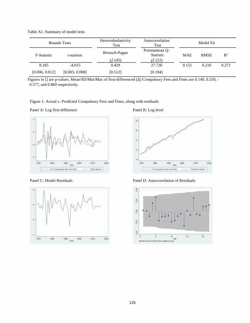
126
Table A1. Summary of model tests
Bounds Tests Hetoroskedasticity
Test Autocorrelation
Test Model Fit
F-Statistic t-statistic Breusch-Pagan Portmanteau Q-
Statistic MAE RMSE R2
χ2 (45) χ2 (22)
8.185 -4.015 0.429 27.730 0.151 0.210 0.271
[0.006, 0.012] [0.003, 0.008] [0.512] [0.184]
Figures in [] are p-values. Mean/SD/Min/Max of first-differenced (∆) Compulsory Fees and Fines are 0.149, 0.250, -
0.577, and 0.869 respectively.
Figure 1. Actual v. Predicted Compulsory Fees and Fines, along with residuals
Panel A: Log first-difference Panel B: Log level
Panel C: Model Residuals Panel D: Autocorrelation of Residuals

127
14. Other Current Transfers, Received
Estimation Period: 1950 – 2016
∆𝑂𝑡ℎ𝑒𝑟 𝐶𝑢𝑟𝑟𝑒𝑛𝑡 𝑇𝑟𝑎𝑛𝑠𝑓𝑒𝑟𝑠, 𝑅𝑒𝑐𝑒𝑖𝑣𝑒𝑑 =−0.241 𝑂𝑡ℎ𝑒𝑟 𝐶𝑢𝑟𝑟𝑒𝑛𝑡 𝑇𝑟𝑎𝑛𝑠𝑓𝑒𝑟𝑠, 𝑅𝑒𝑐𝑒𝑖𝑣𝑒𝑑𝑡−1
(0.072)⏟ 𝐴𝑑𝑗𝑢𝑠𝑡𝑚𝑒𝑛𝑡
+ 0.388(0.243)
+2.150 𝑈𝑆𝐷 𝑁𝑜𝑚𝑖𝑛𝑎𝑙 𝐸𝑥𝑐ℎ𝑎𝑛𝑔𝑒 𝑅𝑎𝑡𝑒𝑡−1(0.302)⏟
𝐿𝑜𝑛𝑔−𝑟𝑢𝑛
+0.519 ∆𝑈𝑆𝐷 𝑁𝑜𝑚𝑖𝑛𝑎𝑙 𝐸𝑥𝑐ℎ𝑎𝑛𝑔𝑒 𝑅𝑎𝑡𝑒
(0.146)⏟ 𝑆ℎ𝑜𝑟𝑡−𝑟𝑢𝑛
Table A1. Summary of model tests
Bounds Tests Hetoroskedasticity
Test Autocorrelation
Test Model Fit
F-Statistic t-statistic Breusch-Pagan Portmanteau Q-
Statistic MAE RMSE R2
χ2 (65) χ2 (33)
6.406 -3.341 0.462 25.405 0.524 0.707 0.166
[0.019, 0.036] [0.016, 0.043] [0.496] [0.824]
Figures in [] are p-values. Mean/SD/Min/Max of first-differenced (∆) Other Current Transfers, Received are 0.123,
0.750, -2.335, and 2.358 respectively.
Figure 1. Actual v. Predicted Other Current Transfers, along with residuals
Panel A: Log first-difference Panel B: Log level

128
Panel C: Model Residuals Panel D: Autocorrelation of Residuals
15. Government Property Income
Estimation Period: 1971 – 2016
∆𝐺𝑜𝑣𝑒𝑟𝑛𝑚𝑒𝑛𝑡 𝑃𝑟𝑜𝑝𝑒𝑟𝑡𝑦 𝐼𝑛𝑐𝑜𝑚𝑒 =−0.352 𝐺𝑜𝑣𝑒𝑟𝑛𝑚𝑒𝑛𝑡 𝑃𝑟𝑜𝑝𝑒𝑟𝑡𝑦 𝐼𝑛𝑐𝑜𝑚𝑒𝑡−1
(0.101)⏟ 𝐴𝑑𝑗𝑢𝑠𝑡𝑚𝑒𝑛𝑡
− 4.372(1.655)
+1.114 𝑊𝑜𝑟𝑙𝑑 𝐺𝐷𝑃,𝑁𝑜𝑚𝑖𝑛𝑎𝑙𝑡−1(0.074)
+0.005 91𝑑𝑎𝑦 𝑇𝐵𝑖𝑙𝑙 𝑅𝑎𝑡𝑒𝑡−1(0.018)⏟
𝐿𝑜𝑛𝑔−𝑟𝑢𝑛
+0.392 ∆𝑊𝑜𝑟𝑙𝑑 𝐺𝐷𝑃,𝑁𝑜𝑚𝑖𝑛𝑎𝑙(0.130)
−0.007 ∆91𝑑𝑎𝑦 𝑇𝐵𝑖𝑙𝑙 𝑅𝑎𝑡𝑒(0.009)
−0.006 ∆91𝑑𝑎𝑦 𝑇𝐵𝑖𝑙𝑙 𝑅𝑎𝑡𝑒𝑡−1(0.008)
−0.040 ∆91𝑑𝑎𝑦 𝑇𝐵𝑖𝑙𝑙 𝑅𝑎𝑡𝑒𝑡−2(0.009)⏟
𝑆ℎ𝑜𝑟𝑡−𝑟𝑢𝑛
Table A1. Summary of model tests
Bounds Tests Hetoroskedasticity
Test Autocorrelation
Test Model Fit
F-Statistic t-statistic Breusch-Pagan Portmanteau Q-
Statistic MAE RMSE R2
χ2 (44) χ2 (22)
7.883 -3.466 0.142 25.385 0.140 0.187 0.525
[0.001, 0.006] [0.013, 0.063] [0.706] [0.279]
Figures in [] are p-values. Mean/SD/Min/Max of first-differenced (∆) Government Property Income are 0.148, 0.276
-0.534, and 0.888 respectively.

129
Figure 1. Actual v. Predicted Government Property Income, along with residuals
Panel A: Log first-difference Panel B: Log level
Panel C: Model Residuals Panel D: Autocorrelation of Residuals
16. Social Security Contributions
Estimation Period: 1981 – 2016
∆𝑆𝑜𝑐𝑖𝑎𝑙 𝑆𝑒𝑐𝑢𝑟𝑖𝑡𝑦 𝐶𝑜𝑛𝑡𝑟𝑖𝑏𝑢𝑡𝑖𝑜𝑛𝑠 =−0.496 𝑆𝑜𝑐𝑖𝑎𝑙 𝑆𝑒𝑐𝑢𝑟𝑖𝑡𝑦 𝐶𝑜𝑛𝑡𝑟𝑖𝑏𝑢𝑡𝑖𝑜𝑛𝑠𝑡−1
(0.112)⏟ 𝐴𝑑𝑗𝑢𝑠𝑡𝑚𝑒𝑛𝑡
+ 5.098(2.797)
+1.036 𝑆𝑜𝑐𝑖𝑎𝑙 𝑆𝑒𝑐𝑢𝑟𝑖𝑡𝑦 𝐵𝑒𝑛𝑒𝑓𝑖𝑡𝑠𝑡−1(0.088)
−0.973 𝐸𝑚𝑝𝑙𝑜𝑦𝑚𝑒𝑛𝑡 𝑖𝑛 𝐼𝑛𝑑𝑢𝑠𝑡𝑟𝑦
(0.448)
+0.118 𝐸𝑚𝑝𝑙𝑜𝑦𝑚𝑒𝑛𝑡 𝑖𝑛 𝑆𝑒𝑟𝑣𝑖𝑐𝑒
(0.252)
−0.356 𝐸𝑚𝑝𝑙𝑜𝑦𝑚𝑒𝑛𝑡 𝑖𝑛 𝐴𝑔𝑟𝑖𝑐𝑢𝑙𝑡𝑢𝑟𝑒
(0.463)⏟ 𝐿𝑜𝑛𝑔−𝑟𝑢𝑛
+0.416 ∆𝑆𝑜𝑐𝑖𝑎𝑙 𝑆𝑒𝑐𝑢𝑟𝑖𝑡𝑦 𝐶𝑜𝑛𝑡𝑟𝑖𝑏𝑢𝑡𝑖𝑜𝑛𝑠𝑡−1(0.113)
+0.358 ∆𝑆𝑜𝑐𝑖𝑎𝑙 𝑆𝑒𝑐𝑢𝑟𝑖𝑡𝑦 𝐶𝑜𝑛𝑡𝑟𝑖𝑏𝑢𝑡𝑖𝑜𝑛𝑠𝑡−2(0.140)
+0.176 ∆𝑆𝑜𝑐𝑖𝑎𝑙 𝑆𝑒𝑐𝑢𝑟𝑖𝑡𝑦 𝐵𝑒𝑛𝑒𝑓𝑖𝑡𝑠
(0.176)−0.386 ∆𝑆𝑜𝑐𝑖𝑎𝑙 𝑆𝑒𝑐𝑢𝑟𝑖𝑡𝑦 𝐵𝑒𝑛𝑒𝑓𝑖𝑡𝑠𝑡−1
(0.144)
−0.302 ∆𝑆𝑜𝑐𝑖𝑎𝑙 𝑆𝑒𝑐𝑢𝑟𝑖𝑡𝑦 𝐵𝑒𝑛𝑒𝑓𝑖𝑡𝑠𝑡−2(0.157)
−0.755 ∆𝐸𝑚𝑝𝑙𝑜𝑦𝑚𝑒𝑛𝑡 𝑖𝑛 𝐴𝑔𝑟𝑖𝑐𝑢𝑙𝑡𝑢𝑟𝑒
(0.291)⏟ 𝑆ℎ𝑜𝑟𝑡−𝑟𝑢𝑛

130
Table A1. Summary of model tests
Bounds Tests Hetoroskedasticity
Test Autocorrelation
Test Model Fit
F-Statistic t-statistic Breusch-Pagan Portmanteau Q-
Statistic MAE RMSE R2
χ2 (34) χ2 (17)
7.548 -4.394 0.199 10.533 0.037 0.064 0.836
[0.001, 0.005] [0.002, 0.028] [0.655] [0.879]
Figures in [] are p-values. Mean/SD/Min/Max of first-differenced (∆) Social Security Contributions are 0.139, 0.097,
-0.050, and 0.369 respectively.
Figure 1. Actual v. Predicted Social Security Contributions, along with residuals
Panel A: Log first-difference Panel B: Log level
Panel C: Model Residuals Panel D: Autocorrelation of Residuals

131
17. Other Current Transfers, Paid
Estimation Period: 1974 – 2016
∆𝑂𝑡ℎ𝑒𝑟 𝐶𝑢𝑟𝑟𝑒𝑛𝑡 𝑇𝑟𝑎𝑛𝑠𝑓𝑒𝑟𝑠, 𝑃𝑎𝑖𝑑 =−0.584 𝑂𝑡ℎ𝑒𝑟 𝐶𝑢𝑟𝑟𝑒𝑛𝑡 𝑇𝑟𝑎𝑛𝑎𝑓𝑒𝑟𝑠, 𝑃𝑎𝑖𝑑𝑡−1
(0.133)⏟ 𝐴𝑑𝑗𝑢𝑠𝑡𝑚𝑒𝑛𝑡
+ 0.708(3.920)
+0.584 𝑊𝑜𝑟𝑙𝑑 𝐺𝐷𝑃,𝑁𝑜𝑚𝑖𝑛𝑎𝑙(0.303)
−0.985 𝑈𝑆𝐷 𝑁𝑜𝑚𝑖𝑛𝑎𝑙 𝐸𝑥𝑐ℎ𝑎𝑛𝑔𝑒 𝑅𝑎𝑡𝑒
(0.641)+0.826 𝐽𝑃𝑌 𝑁𝑜𝑚𝑖𝑛𝑎𝑙 𝐸𝑥𝑐ℎ𝑎𝑛𝑔𝑒 𝑅𝑎𝑡𝑒
(0.518)⏟ 𝐿𝑜𝑛𝑔−𝑟𝑢𝑛
+ ∆( )
+ ∆( )⏟
𝑆ℎ𝑜𝑟𝑡−𝑟𝑢𝑛
Table A1. Summary of model tests
Bounds Tests Hetoroskedasticity
Test Autocorrelation
Test Model Fit
F-Statistic t-statistic Breusch-Pagan Portmanteau Q-
Statistic MAE RMSE R2
χ2 (41) χ2 (21)
5.135 -4.386 1.365 20.241 0.207 0.256 0.350
[0.008, 0.034] [0.001, 0.016] [0.242] [0.506]
Figures in [] are p-values. Mean/SD/Min/Max of first-differenced (∆) Other Current Transfers, Paid are 0.105, 0.326,
-0.673, and 1.410 respectively.
Figure 1. Actual v. Predicted Other Current Transfers, along with residuals
Panel A: Log first-difference Panel B: Log level
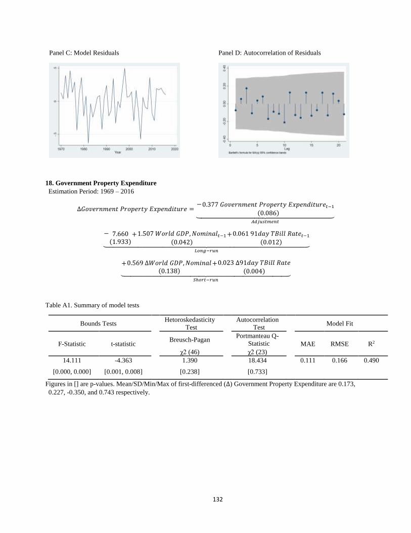
132
Panel C: Model Residuals Panel D: Autocorrelation of Residuals
18. Government Property Expenditure
Estimation Period: 1969 – 2016
∆𝐺𝑜𝑣𝑒𝑟𝑛𝑚𝑒𝑛𝑡 𝑃𝑟𝑜𝑝𝑒𝑟𝑡𝑦 𝐸𝑥𝑝𝑒𝑛𝑑𝑖𝑡𝑢𝑟𝑒 =−0.377 𝐺𝑜𝑣𝑒𝑟𝑛𝑚𝑒𝑛𝑡 𝑃𝑟𝑜𝑝𝑒𝑟𝑡𝑦 𝐸𝑥𝑝𝑒𝑛𝑑𝑖𝑡𝑢𝑟𝑒𝑡−1
(0.086)⏟ 𝐴𝑑𝑗𝑢𝑠𝑡𝑚𝑒𝑛𝑡
− 7.660(1.933)
+1.507 𝑊𝑜𝑟𝑙𝑑 𝐺𝐷𝑃,𝑁𝑜𝑚𝑖𝑛𝑎𝑙𝑡−1(0.042)
+0.061 91𝑑𝑎𝑦 𝑇𝐵𝑖𝑙𝑙 𝑅𝑎𝑡𝑒𝑡−1(0.012)⏟
𝐿𝑜𝑛𝑔−𝑟𝑢𝑛
+0.569 ∆𝑊𝑜𝑟𝑙𝑑 𝐺𝐷𝑃,𝑁𝑜𝑚𝑖𝑛𝑎𝑙(0.138)
+0.023 ∆91𝑑𝑎𝑦 𝑇𝐵𝑖𝑙𝑙 𝑅𝑎𝑡𝑒(0.004)⏟
𝑆ℎ𝑜𝑟𝑡−𝑟𝑢𝑛
Table A1. Summary of model tests
Bounds Tests Hetoroskedasticity
Test Autocorrelation
Test Model Fit
F-Statistic t-statistic Breusch-Pagan Portmanteau Q-
Statistic MAE RMSE R2
χ2 (46) χ2 (23)
14.111 -4.363 1.390 18.434 0.111 0.166 0.490
[0.000, 0.000] [0.001, 0.008] [0.238] [0.733]
Figures in [] are p-values. Mean/SD/Min/Max of first-differenced (∆) Government Property Expenditure are 0.173,
0.227, -0.350, and 0.743 respectively.
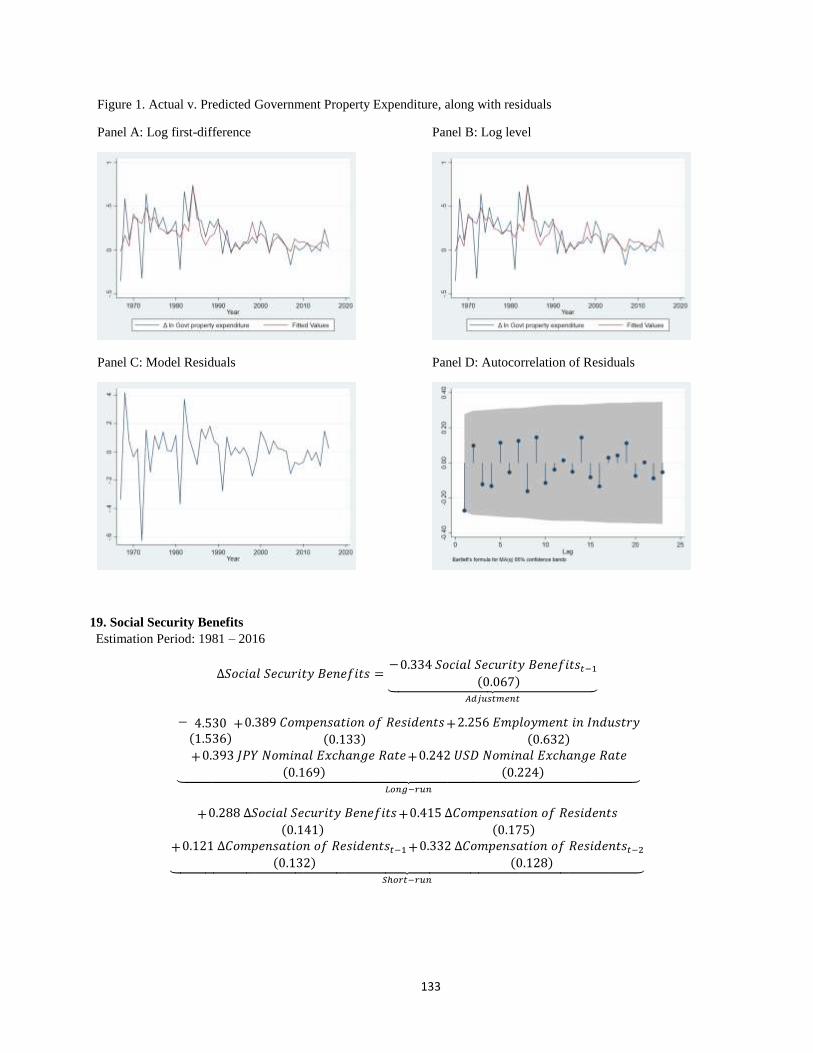
133
Figure 1. Actual v. Predicted Government Property Expenditure, along with residuals
Panel A: Log first-difference Panel B: Log level
Panel C: Model Residuals Panel D: Autocorrelation of Residuals
19. Social Security Benefits
Estimation Period: 1981 – 2016
∆𝑆𝑜𝑐𝑖𝑎𝑙 𝑆𝑒𝑐𝑢𝑟𝑖𝑡𝑦 𝐵𝑒𝑛𝑒𝑓𝑖𝑡𝑠 =−0.334 𝑆𝑜𝑐𝑖𝑎𝑙 𝑆𝑒𝑐𝑢𝑟𝑖𝑡𝑦 𝐵𝑒𝑛𝑒𝑓𝑖𝑡𝑠𝑡−1
(0.067)⏟ 𝐴𝑑𝑗𝑢𝑠𝑡𝑚𝑒𝑛𝑡
− 4.530(1.536)
+0.389 𝐶𝑜𝑚𝑝𝑒𝑛𝑠𝑎𝑡𝑖𝑜𝑛 𝑜𝑓 𝑅𝑒𝑠𝑖𝑑𝑒𝑛𝑡𝑠
(0.133)+2.256 𝐸𝑚𝑝𝑙𝑜𝑦𝑚𝑒𝑛𝑡 𝑖𝑛 𝐼𝑛𝑑𝑢𝑠𝑡𝑟𝑦
(0.632)
+0.393 𝐽𝑃𝑌 𝑁𝑜𝑚𝑖𝑛𝑎𝑙 𝐸𝑥𝑐ℎ𝑎𝑛𝑔𝑒 𝑅𝑎𝑡𝑒
(0.169)+0.242 𝑈𝑆𝐷 𝑁𝑜𝑚𝑖𝑛𝑎𝑙 𝐸𝑥𝑐ℎ𝑎𝑛𝑔𝑒 𝑅𝑎𝑡𝑒
(0.224)⏟ 𝐿𝑜𝑛𝑔−𝑟𝑢𝑛
+0.288 ∆𝑆𝑜𝑐𝑖𝑎𝑙 𝑆𝑒𝑐𝑢𝑟𝑖𝑡𝑦 𝐵𝑒𝑛𝑒𝑓𝑖𝑡𝑠
(0.141)+0.415 ∆𝐶𝑜𝑚𝑝𝑒𝑛𝑠𝑎𝑡𝑖𝑜𝑛 𝑜𝑓 𝑅𝑒𝑠𝑖𝑑𝑒𝑛𝑡𝑠
(0.175)
+0.121 ∆𝐶𝑜𝑚𝑝𝑒𝑛𝑠𝑎𝑡𝑖𝑜𝑛 𝑜𝑓 𝑅𝑒𝑠𝑖𝑑𝑒𝑛𝑡𝑠𝑡−1(0.132)
+0.332 ∆𝐶𝑜𝑚𝑝𝑒𝑛𝑠𝑎𝑡𝑖𝑜𝑛 𝑜𝑓 𝑅𝑒𝑠𝑖𝑑𝑒𝑛𝑡𝑠𝑡−2(0.128)⏟
𝑆ℎ𝑜𝑟𝑡−𝑟𝑢𝑛

134
Table A1. Summary of model tests
Bounds Tests Hetoroskedasticity
Test Autocorrelation
Test Model Fit
F-Statistic t-statistic Breusch-Pagan Portmanteau Q-
Statistic MAE RMSE R2
χ2 (34) χ2 (17)
5.805 -4.939 1.814 23.404 0.040 0.054 0.664
[0.003, 0.019] [0.000, 0.010] [0.177] [0.136]
Figures in [] are p-values. Mean/SD/Min/Max of first-differenced (∆) Social Security Benefits are 0.185, 0.110,
0.016, and 0.606 respectively.
Figure 1. Actual v. Predicted Social Security Benefits, along with residuals
Panel A: Log first-difference Panel B: Log level
Panel C: Model Residuals Panel D: Autocorrelation of Residuals

135
20. Implicit Price Index, Government Spending
Estimation Period: 1981 – 2016
∆𝐼𝑃𝐼𝑁, 𝐺𝑜𝑣𝑒𝑟𝑛𝑚𝑒𝑛𝑡 𝑆𝑝𝑒𝑛𝑑𝑖𝑛𝑔 =−0.376 𝐼𝑃𝐼𝑁, 𝐺𝑜𝑣𝑒𝑟𝑛𝑚𝑒𝑛𝑡 𝑆𝑝𝑒𝑛𝑑𝑖𝑛𝑔𝑡−1
(0.090)⏟ 𝐴𝑑𝑗𝑢𝑠𝑡𝑚𝑒𝑛𝑡
− 2.264(0.591)
+0.291 𝑊𝑎𝑔𝑒 𝐼𝑛𝑑𝑒𝑥, 𝑃𝑟𝑖𝑣𝑎𝑡𝑒 𝑆𝑒𝑟𝑣𝑖𝑐𝑒𝑡−1(0.075)
+1.007 𝐶𝑃𝐼𝑡−1(0.036)⏟
𝐿𝑜𝑛𝑔−𝑟𝑢𝑛
+0.493 ∆𝐼𝑃𝐼𝑁, 𝐺𝑜𝑣𝑒𝑟𝑛𝑚𝑒𝑛𝑡 𝑆𝑝𝑒𝑛𝑑𝑖𝑛𝑔𝑡−1(0.118)
+0.110 ∆𝑊𝑎𝑔𝑒 𝐼𝑛𝑑𝑒𝑥, 𝑃𝑟𝑖𝑣𝑎𝑡𝑒 𝑆𝑒𝑟𝑣𝑖𝑐𝑒
(0.042)
+0.704 ∆𝐶𝑃𝐼(0.073)
−0.406 ∆𝐶𝑃𝐼𝑡−1(0.104)⏟
𝑆ℎ𝑜𝑟𝑡−𝑟𝑢𝑛
Table A1. Summary of model tests
Bounds Tests Hetoroskedasticity
Test Autocorrelation
Test Model Fit
F-Statistic t-statistic Breusch-Pagan Portmanteau Q-
Statistic MAE RMSE R2
χ2 (34) χ2 (16)
7.277 -4.185 0.030 23.819 0.015 0.020 0.894
[0.004, 0.013] [0.002, 0.016] [0.860] [0.093]
Figures in [] are p-values. Mean/SD/Min/Max of first-differenced (∆) Implicit Price Index, Government Spending are
0.069, 0.074, -0.256, and 0.326 respectively.
Figure 1. Actual v. Predicted Implicit Price Index, Government Spending, along with residuals
Panel A: Log first-difference Panel B: Log level

136
Panel C: Model Residuals Panel D: Autocorrelation of Residuals
Trade Sector
1. Implicit Price Index – Agricultural Imports
Estimation Period: 1974 – 2017
∆𝐼𝑃𝐼𝑁, 𝐴𝑔𝑟𝑖𝑐𝑢𝑙𝑡𝑢𝑟𝑎𝑙 𝐼𝑚𝑝𝑜𝑟𝑡𝑠 =−0.788 𝐼𝑃𝐼𝑁, 𝐴𝑔𝑟𝑖𝑐𝑢𝑙𝑡𝑢𝑟𝑎𝑙 𝐼𝑚𝑝𝑜𝑟𝑡𝑠𝑡−1
(0.119)⏟ 𝐴𝑑𝑗𝑢𝑠𝑡𝑚𝑒𝑛𝑡
− 5.041(2.016)
+0.964 𝐹𝑜𝑟𝑒𝑖𝑔𝑛 𝐼𝑃𝐼𝑁, 𝐴𝑔𝑟𝑖𝑐𝑢𝑙𝑡𝑢𝑟𝑎𝑙 𝐼𝑚𝑝𝑜𝑟𝑡𝑠
(0.193)+1.178 𝑈𝑆𝐷 𝑁𝑜𝑚𝑖𝑛𝑎𝑙 𝐸𝑥𝑐ℎ𝑎𝑛𝑔𝑒 𝑅𝑎𝑡𝑒
(0.387)−0.048 𝐽𝑃𝑌 𝑁𝑜𝑚𝑖𝑛𝑎𝑙 𝐸𝑥𝑐ℎ𝑎𝑛𝑔𝑒 𝑅𝑎𝑡𝑒
(0.218)
−0.208 𝐶𝑁𝑌 𝑁𝑜𝑚𝑖𝑛𝑎𝑙 𝐸𝑥𝑐ℎ𝑎𝑛𝑔𝑒 𝑅𝑎𝑡𝑒
(0.149)−0.499 𝑇𝑎𝑟𝑖𝑓𝑓, 𝐴𝑔𝑟𝑖𝑐𝑢𝑙𝑡𝑢𝑟𝑎𝑙 𝐼𝑚𝑝𝑜𝑟𝑡𝑠
(0.140)
−0.227 𝑃ℎ𝑖𝑙𝑖𝑝𝑝𝑖𝑛𝑒 𝑅𝑒𝑡𝑎𝑖𝑙 𝑃𝑟𝑖𝑐𝑒 𝐼𝑛𝑑𝑒𝑥
(0.165)⏟ 𝐿𝑜𝑛𝑔−𝑟𝑢𝑛
+0.210 ∆𝐼𝑚𝑝𝑜𝑟𝑡 𝐷𝑢𝑡𝑖𝑒𝑠(0.126)⏟
𝑆ℎ𝑜𝑟𝑡−𝑟𝑢𝑛
Table A1. Summary of model tests
Bounds Tests Hetoroskedasticity
Test Autocorrelation
Test Model Fit
F-Statistic t-statistic Breusch-Pagan Portmanteau Q-
Statistic MAE RMSE R2
χ2 (42) χ2 (22)
6.711 -6.574 1.685 15.655 0.087 0.114 0.579
[0.000, 0.003] [0.000, 0.001] [0.194] [0.832]
Figures in [] are p-values. Mean/SD/Min/Max of first-differenced (∆) IPIN – Agricultural Imports are 0.074, 0.169, -
0.301, and 0.487 respectively.
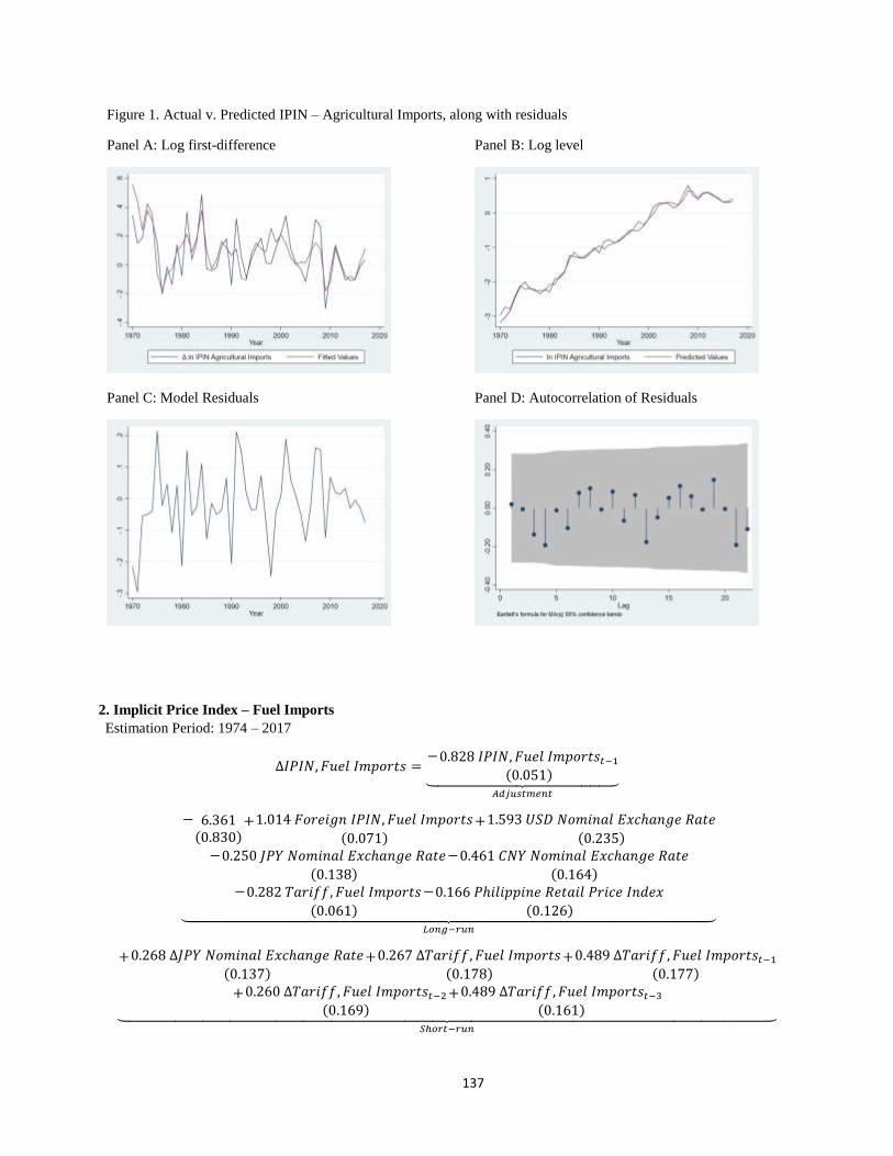
137
Figure 1. Actual v. Predicted IPIN – Agricultural Imports, along with residuals
Panel A: Log first-difference Panel B: Log level
Panel C: Model Residuals Panel D: Autocorrelation of Residuals
2. Implicit Price Index – Fuel Imports
Estimation Period: 1974 – 2017
∆𝐼𝑃𝐼𝑁, 𝐹𝑢𝑒𝑙 𝐼𝑚𝑝𝑜𝑟𝑡𝑠 =−0.828 𝐼𝑃𝐼𝑁, 𝐹𝑢𝑒𝑙 𝐼𝑚𝑝𝑜𝑟𝑡𝑠𝑡−1
(0.051)⏟ 𝐴𝑑𝑗𝑢𝑠𝑡𝑚𝑒𝑛𝑡
− 6.361(0.830)
+1.014 𝐹𝑜𝑟𝑒𝑖𝑔𝑛 𝐼𝑃𝐼𝑁, 𝐹𝑢𝑒𝑙 𝐼𝑚𝑝𝑜𝑟𝑡𝑠
(0.071)+1.593 𝑈𝑆𝐷 𝑁𝑜𝑚𝑖𝑛𝑎𝑙 𝐸𝑥𝑐ℎ𝑎𝑛𝑔𝑒 𝑅𝑎𝑡𝑒
(0.235)−0.250 𝐽𝑃𝑌 𝑁𝑜𝑚𝑖𝑛𝑎𝑙 𝐸𝑥𝑐ℎ𝑎𝑛𝑔𝑒 𝑅𝑎𝑡𝑒
(0.138)
−0.461 𝐶𝑁𝑌 𝑁𝑜𝑚𝑖𝑛𝑎𝑙 𝐸𝑥𝑐ℎ𝑎𝑛𝑔𝑒 𝑅𝑎𝑡𝑒
(0.164)−0.282 𝑇𝑎𝑟𝑖𝑓𝑓, 𝐹𝑢𝑒𝑙 𝐼𝑚𝑝𝑜𝑟𝑡𝑠
(0.061)
−0.166 𝑃ℎ𝑖𝑙𝑖𝑝𝑝𝑖𝑛𝑒 𝑅𝑒𝑡𝑎𝑖𝑙 𝑃𝑟𝑖𝑐𝑒 𝐼𝑛𝑑𝑒𝑥
(0.126)⏟ 𝐿𝑜𝑛𝑔−𝑟𝑢𝑛
+0.268 ∆𝐽𝑃𝑌 𝑁𝑜𝑚𝑖𝑛𝑎𝑙 𝐸𝑥𝑐ℎ𝑎𝑛𝑔𝑒 𝑅𝑎𝑡𝑒
(0.137)+0.267 ∆𝑇𝑎𝑟𝑖𝑓𝑓, 𝐹𝑢𝑒𝑙 𝐼𝑚𝑝𝑜𝑟𝑡𝑠
(0.178)+0.489 ∆𝑇𝑎𝑟𝑖𝑓𝑓, 𝐹𝑢𝑒𝑙 𝐼𝑚𝑝𝑜𝑟𝑡𝑠𝑡−1
(0.177)
+0.260 ∆𝑇𝑎𝑟𝑖𝑓𝑓, 𝐹𝑢𝑒𝑙 𝐼𝑚𝑝𝑜𝑟𝑡𝑠𝑡−2(0.169)
+0.489 ∆𝑇𝑎𝑟𝑖𝑓𝑓, 𝐹𝑢𝑒𝑙 𝐼𝑚𝑝𝑜𝑟𝑡𝑠𝑡−3(0.161)⏟
𝑆ℎ𝑜𝑟𝑡−𝑟𝑢𝑛
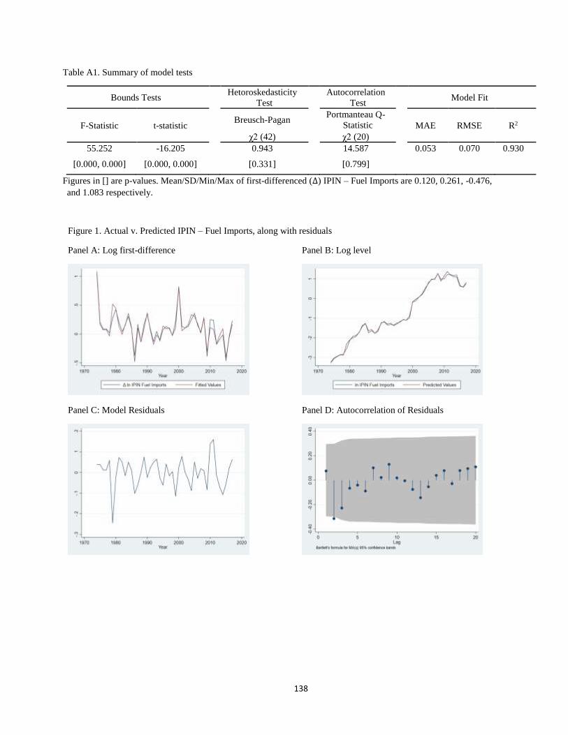
138
Table A1. Summary of model tests
Bounds Tests Hetoroskedasticity
Test Autocorrelation
Test Model Fit
F-Statistic t-statistic Breusch-Pagan Portmanteau Q-
Statistic MAE RMSE R2
χ2 (42) χ2 (20)
55.252 -16.205 0.943 14.587 0.053 0.070 0.930
[0.000, 0.000] [0.000, 0.000] [0.331] [0.799]
Figures in [] are p-values. Mean/SD/Min/Max of first-differenced (∆) IPIN – Fuel Imports are 0.120, 0.261, -0.476,
and 1.083 respectively.
Figure 1. Actual v. Predicted IPIN – Fuel Imports, along with residuals
Panel A: Log first-difference Panel B: Log level
Panel C: Model Residuals Panel D: Autocorrelation of Residuals

139
3. Implicit Price Index – Machinery Imports
Estimation Period: 1974 – 2017
∆𝐼𝑃𝐼𝑁,𝑀𝑎𝑐ℎ𝑖𝑛𝑒𝑟𝑦 𝐼𝑚𝑝𝑜𝑟𝑡𝑠 =−0.547 𝐼𝑃𝐼𝑁,𝑀𝑎𝑐ℎ𝑖𝑛𝑒𝑟𝑦 𝐼𝑚𝑝𝑜𝑟𝑡𝑠𝑡−1
(0.112)⏟ 𝐴𝑑𝑗𝑢𝑠𝑡𝑚𝑒𝑛𝑡
− 1.688(0.443)
+1.243 𝑈𝑆𝐷 𝑁𝑜𝑚𝑖𝑛𝑎𝑙 𝐸𝑥𝑐ℎ𝑎𝑛𝑔𝑒 𝑅𝑎𝑡𝑒
(0.101)
−0.879 𝐶𝑁𝑌 𝑁𝑜𝑚𝑖𝑛𝑎𝑙 𝐸𝑥𝑐ℎ𝑎𝑛𝑔𝑒 𝑅𝑎𝑡𝑒
(0.200)+0.139 𝐼𝑃𝐼𝑁, 𝐹𝑢𝑒𝑙 𝐼𝑚𝑝𝑜𝑟𝑡𝑠
(0.065)⏟ 𝐿𝑜𝑛𝑔−𝑟𝑢𝑛
+0.411 ∆𝐶𝑁𝑌 𝑁𝑜𝑚𝑖𝑛𝑎𝑙 𝐸𝑥𝑐ℎ𝑎𝑛𝑔𝑒 𝑅𝑎𝑡𝑒
(0.157)+0.615 ∆𝐶𝑁𝑌 𝑁𝑜𝑚𝑖𝑛𝑎𝑙 𝐸𝑥𝑐ℎ𝑎𝑛𝑔𝑒 𝑅𝑎𝑡𝑒𝑡−1
(0.157)+0.192 ∆𝐼𝑃𝐼𝑁, 𝐹𝑢𝑒𝑙 𝐼𝑚𝑝𝑜𝑟𝑡𝑠
(0.066)⏟ 𝑆ℎ𝑜𝑟𝑡−𝑟𝑢𝑛
Table A1. Summary of model tests
Bounds Tests Hetoroskedasticity
Test Autocorrelation
Test Model Fit
F-Statistic t-statistic Breusch-Pagan Portmanteau Q-
Statistic MAE RMSE R2
χ2 (42) χ2 (21)
8.908 -4.851 2.636 17.410 0.085 0.127 0.619
[0.000, 0.001] [0.000, 0.005] [0.104] [0.685]
Figures in [] are p-values. Mean/SD/Min/Max of first-differenced (∆) IPIN – Machinery Imports are 0.073, 0.168, -
0.573, and 0.168 respectively.
Figure 1. Actual v. Predicted IPIN – Machinery Imports, along with residuals
Panel A: Log first-difference Panel B: Log level

140
Panel C: Model Residuals Panel D: Autocorrelation of Residuals
4. Implicit Price Index – Materials Imports
Estimation Period: 1990 – 2016
∆𝐼𝑃𝐼𝑁,𝑀𝑎𝑡𝑒𝑟𝑖𝑎𝑙𝑠 𝐼𝑚𝑝𝑜𝑟𝑡𝑠 =−0.355 𝐼𝑃𝐼𝑁,𝑀𝑎𝑡𝑒𝑟𝑖𝑎𝑙𝑠 𝐼𝑚𝑝𝑜𝑟𝑡𝑠𝑡−1
(0.086)⏟ 𝐴𝑑𝑗𝑢𝑠𝑡𝑚𝑒𝑛𝑡
+ 5.126(1.474)
−2.223 𝐹𝑜𝑟𝑒𝑖𝑔𝑛 𝐼𝑃𝐼𝑁,𝑀𝑎𝑡𝑒𝑟𝑖𝑎𝑙𝑠 𝐼𝑚𝑝𝑜𝑟𝑡𝑠
(0.800)
−2.087 𝑈𝑆𝐷 𝑁𝑜𝑚𝑖𝑛𝑎𝑙 𝐸𝑥𝑐ℎ𝑎𝑛𝑔𝑒 𝑅𝑎𝑡𝑒
(0.103)
+1.554 𝐽𝑃𝑌 𝑁𝑜𝑚𝑖𝑛𝑎𝑙 𝐸𝑥𝑐ℎ𝑎𝑛𝑔𝑒 𝑅𝑎𝑡𝑒
(0.502)+0.140 𝐶𝑁𝑌 𝑁𝑜𝑚𝑖𝑛𝑎𝑙 𝐸𝑥𝑐ℎ𝑎𝑛𝑔𝑒 𝑅𝑎𝑡𝑒
(0.171)−0.242 𝑇𝑎𝑟𝑖𝑓𝑓,𝑀𝑎𝑡𝑒𝑟𝑖𝑎𝑙𝑠 𝐼𝑚𝑝𝑜𝑟𝑡𝑠
(0.135)+1.112 𝑃ℎ𝑖𝑙𝑖𝑝𝑝𝑖𝑛𝑒 𝑅𝑒𝑡𝑎𝑖𝑙 𝑃𝑟𝑖𝑐𝑒 𝐼𝑛𝑑𝑒𝑧
(0.543)⏟ 𝐿𝑜𝑛𝑔−𝑟𝑢𝑛
+0.430 ∆𝐹𝑜𝑟𝑒𝑖𝑔𝑛 𝐼𝑃𝐼𝑁,𝑀𝑎𝑡𝑒𝑟𝑖𝑎𝑙𝑠 𝐼𝑚𝑝𝑜𝑟𝑡𝑠
(0.178)+0.357 ∆𝐹𝑜𝑟𝑒𝑖𝑔𝑛 𝐼𝑃𝐼𝑁,𝑀𝑎𝑡𝑒𝑟𝑖𝑎𝑙𝑠 𝐼𝑚𝑝𝑜𝑟𝑡𝑠𝑡−1
(0.122)
+0.869 ∆𝑈𝑆𝐷 𝑁𝑜𝑚𝑖𝑛𝑎𝑙 𝐸𝑥𝑐ℎ𝑎𝑛𝑔𝑒 𝑅𝑎𝑡𝑒
(0.214)
−0.210 ∆𝐽𝑃𝑌 𝑁𝑜𝑚𝑖𝑛𝑎𝑙 𝐸𝑥𝑐ℎ𝑎𝑛𝑔𝑒 𝑅𝑎𝑡𝑒
(0.122)
+0.357 ∆𝑃ℎ𝑖𝑙𝑖𝑝𝑝𝑖𝑛𝑒 𝑅𝑒𝑡𝑎𝑖𝑙 𝑃𝑟𝑖𝑐𝑒 𝐼𝑛𝑑𝑒𝑥
(0.172)⏟ 𝑆ℎ𝑜𝑟𝑡−𝑟𝑢𝑛
Table A1. Summary of model tests
Bounds Tests Hetoroskedasticity
Test Autocorrelation
Test Model Fit
F-Statistic t-statistic Breusch-Pagan Portmanteau Q-
Statistic MAE RMSE R2
χ2 (42) χ2 (21)
6.776 -4.105 0.048 10.318 0.054 0.088 0.858
[0.000, 0.003] [0.003, 0.082] [0.826] [0.974]
Figures in [] are p-values. Mean/SD/Min/Max of first-differenced (∆) IPIN – Materials Imports are 0.070, 0.150, -
0.143, and 0.541 respectively.
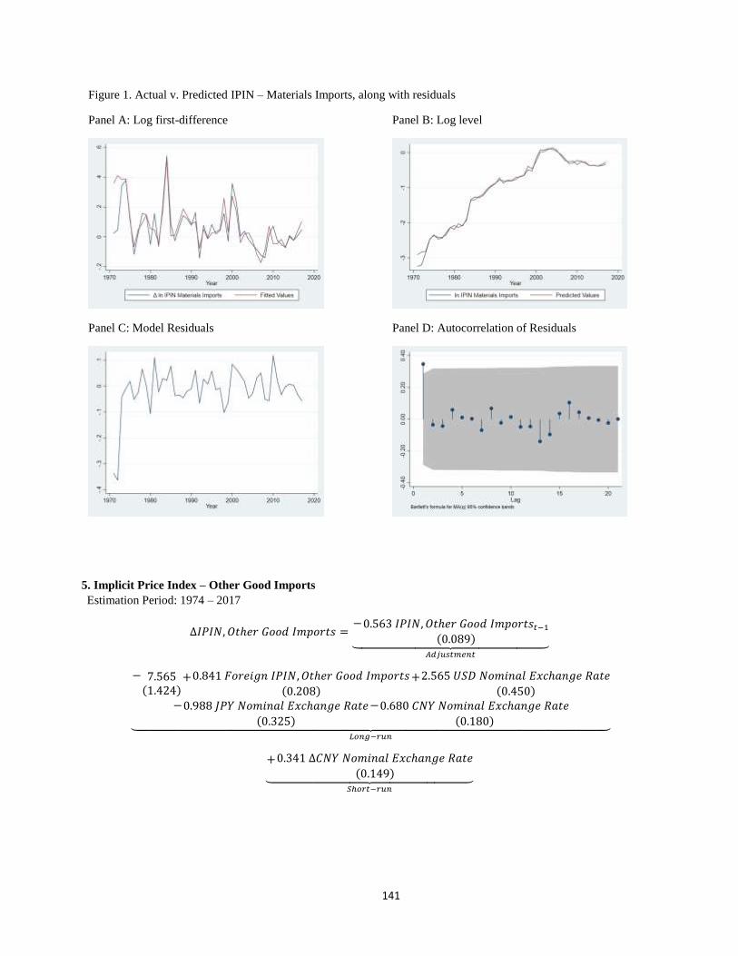
141
Figure 1. Actual v. Predicted IPIN – Materials Imports, along with residuals
Panel A: Log first-difference Panel B: Log level
Panel C: Model Residuals Panel D: Autocorrelation of Residuals
5. Implicit Price Index – Other Good Imports
Estimation Period: 1974 – 2017
∆𝐼𝑃𝐼𝑁, 𝑂𝑡ℎ𝑒𝑟 𝐺𝑜𝑜𝑑 𝐼𝑚𝑝𝑜𝑟𝑡𝑠 =−0.563 𝐼𝑃𝐼𝑁, 𝑂𝑡ℎ𝑒𝑟 𝐺𝑜𝑜𝑑 𝐼𝑚𝑝𝑜𝑟𝑡𝑠𝑡−1
(0.089)⏟ 𝐴𝑑𝑗𝑢𝑠𝑡𝑚𝑒𝑛𝑡
− 7.565(1.424)
+0.841 𝐹𝑜𝑟𝑒𝑖𝑔𝑛 𝐼𝑃𝐼𝑁, 𝑂𝑡ℎ𝑒𝑟 𝐺𝑜𝑜𝑑 𝐼𝑚𝑝𝑜𝑟𝑡𝑠
(0.208)+2.565 𝑈𝑆𝐷 𝑁𝑜𝑚𝑖𝑛𝑎𝑙 𝐸𝑥𝑐ℎ𝑎𝑛𝑔𝑒 𝑅𝑎𝑡𝑒
(0.450)−0.988 𝐽𝑃𝑌 𝑁𝑜𝑚𝑖𝑛𝑎𝑙 𝐸𝑥𝑐ℎ𝑎𝑛𝑔𝑒 𝑅𝑎𝑡𝑒
(0.325)
−0.680 𝐶𝑁𝑌 𝑁𝑜𝑚𝑖𝑛𝑎𝑙 𝐸𝑥𝑐ℎ𝑎𝑛𝑔𝑒 𝑅𝑎𝑡𝑒
(0.180)⏟ 𝐿𝑜𝑛𝑔−𝑟𝑢𝑛
+0.341 ∆𝐶𝑁𝑌 𝑁𝑜𝑚𝑖𝑛𝑎𝑙 𝐸𝑥𝑐ℎ𝑎𝑛𝑔𝑒 𝑅𝑎𝑡𝑒
(0.149)⏟ 𝑆ℎ𝑜𝑟𝑡−𝑟𝑢𝑛

142
Table A1. Summary of model tests
Bounds Tests Hetoroskedasticity
Test Autocorrelation
Test Model Fit
F-Statistic t-statistic Breusch-Pagan Portmanteau Q-
Statistic MAE RMSE R2
χ2 (42) χ2 (21)
10.962 -6.288 0.132 18.453 0.077 0.102 0.622
[0.000, 0.000] [0.000, 0.000] [0.715] [0.620]
Figures in [] are p-values. Mean/SD/Min/Max of first-differenced (∆) IPIN – Other Good Imports are 0.078, 0.201, -
0.312, and 0.948 respectively.
Figure 1. Actual v. Predicted IPIN – Other Good Imports, along with residuals
Panel A: Log first-difference Panel B: Log level
Panel C: Model Residuals Panel D: Autocorrelation of Residuals
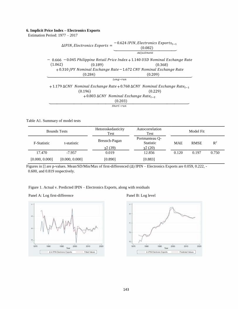
143
6. Implicit Price Index – Electronics Exports
Estimation Period: 1977 – 2017
∆𝐼𝑃𝐼𝑁, 𝐸𝑙𝑒𝑐𝑡𝑟𝑜𝑛𝑖𝑐𝑠 𝐸𝑥𝑝𝑜𝑟𝑡𝑠 =−0.624 𝐼𝑃𝐼𝑁, 𝐸𝑙𝑒𝑐𝑡𝑟𝑜𝑛𝑖𝑐𝑠 𝐸𝑥𝑝𝑜𝑟𝑡𝑠𝑡−1
(0.082)⏟ 𝐴𝑑𝑗𝑢𝑠𝑡𝑚𝑒𝑛𝑡
− 0.666(1.062)
−0.045 𝑃ℎ𝑖𝑙𝑖𝑝𝑝𝑖𝑛𝑒 𝑅𝑒𝑡𝑎𝑖𝑙 𝑃𝑟𝑖𝑐𝑒 𝐼𝑛𝑑𝑒𝑥
(0.189)+1.140 𝑈𝑆𝐷 𝑁𝑜𝑚𝑖𝑛𝑎𝑙 𝐸𝑥𝑐ℎ𝑎𝑛𝑔𝑒 𝑅𝑎𝑡𝑒
(0.368)
+0.310 𝐽𝑃𝑌 𝑁𝑜𝑚𝑖𝑛𝑎𝑙 𝐸𝑥𝑐ℎ𝑎𝑛𝑔𝑒 𝑅𝑎𝑡𝑒
(0.284)
−1.672 𝐶𝑁𝑌 𝑁𝑜𝑚𝑖𝑛𝑎𝑙 𝐸𝑥𝑐ℎ𝑎𝑛𝑔𝑒 𝑅𝑎𝑡𝑒
(0.209)⏟ 𝐿𝑜𝑛𝑔−𝑟𝑢𝑛
+1.179 ∆𝐶𝑁𝑌 𝑁𝑜𝑚𝑖𝑛𝑎𝑙 𝐸𝑥𝑐ℎ𝑎𝑛𝑔𝑒 𝑅𝑎𝑡𝑒
(0.196)+0.768 ∆𝐶𝑁𝑌 𝑁𝑜𝑚𝑖𝑛𝑎𝑙 𝐸𝑥𝑐ℎ𝑎𝑛𝑔𝑒 𝑅𝑎𝑡𝑒𝑡−1
(0.229)
+0.803 ∆𝐶𝑁𝑌 𝑁𝑜𝑚𝑖𝑛𝑎𝑙 𝐸𝑥𝑐ℎ𝑎𝑛𝑔𝑒 𝑅𝑎𝑡𝑒𝑡−2(0.203)⏟
𝑆ℎ𝑜𝑟𝑡−𝑟𝑢𝑛
Table A1. Summary of model tests
Bounds Tests Hetoroskedasticity
Test Autocorrelation
Test Model Fit
F-Statistic t-statistic Breusch-Pagan Portmanteau Q-
Statistic MAE RMSE R2
χ2 (39) χ2 (20)
17.470 -7.957 0.019 12.856 0.120 0.197 0.750
[0.000, 0.000] [0.000, 0.000] [0.890] [0.883]
Figures in [] are p-values. Mean/SD/Min/Max of first-differenced (∆) IPIN – Electronics Exports are 0.059, 0.222, -
0.600, and 0.819 respectively.
Figure 1. Actual v. Predicted IPIN – Electronics Exports, along with residuals
Panel A: Log first-difference Panel B: Log level

144
Panel C: Model Residuals Panel D: Autocorrelation of Residuals
7. Implicit Price Index – Agricultural Exports
Estimation Period: 1974 – 2017
∆𝐼𝑃𝐼𝑁, 𝐴𝑔𝑟𝑖𝑐𝑢𝑙𝑡𝑢𝑟𝑎𝑙 𝐸𝑥𝑝𝑜𝑟𝑡𝑠 =−0.546 𝐼𝑃𝐼𝑁, 𝐴𝑔𝑟𝑖𝑐𝑢𝑙𝑡𝑢𝑟𝑎𝑙 𝐸𝑥𝑝𝑜𝑟𝑡𝑠𝑡−1
(0.134)⏟ 𝐴𝑑𝑗𝑢𝑠𝑡𝑚𝑒𝑛𝑡
− 4.158(1.127)
+0.764 𝑊𝑜𝑟𝑙𝑑 𝑊ℎ𝑜𝑙𝑒𝑠𝑎𝑙𝑒 𝑃𝑟𝑖𝑐𝑒 𝐼𝑛𝑑𝑒𝑥𝑡−1(0.107)
+0.813 𝑈𝑆𝐷 𝑁𝑜𝑚𝑖𝑛𝑎𝑙 𝐸𝑥𝑐ℎ𝑎𝑛𝑔𝑒 𝑅𝑎𝑡𝑒𝑡−1(0.509)
+0.502 𝐶𝑁𝑌 𝑁𝑜𝑚𝑖𝑛𝑎𝑙 𝐸𝑥𝑐ℎ𝑎𝑛𝑔𝑒 𝑅𝑎𝑡𝑒𝑡−1(0.240)
−0.529 𝐽𝑃𝑌 𝑁𝑜𝑚𝑖𝑛𝑎𝑙 𝐸𝑥ℎ𝑎𝑛𝑔𝑒 𝑅𝑎𝑡𝑒𝑡−1(0.367)⏟
𝐿𝑜𝑛𝑔−𝑟𝑢𝑛
+1.173 ∆𝑊𝑜𝑟𝑙𝑑 𝑊ℎ𝑜𝑙𝑒𝑠𝑎𝑙𝑒 𝑃𝑟𝑖𝑐𝑒 𝐼𝑛𝑑𝑒𝑥(0.537)
−0.322 ∆𝑊𝑜𝑟𝑙𝑑 𝑊ℎ𝑜𝑙𝑒𝑠𝑎𝑙𝑒 𝑃𝑟𝑖𝑐𝑒 𝐼𝑛𝑑𝑒𝑥𝑡−1(0.507)
−1.936 ∆𝑊𝑜𝑟𝑙𝑑 𝑊ℎ𝑜𝑙𝑒𝑠𝑎𝑙𝑒 𝑃𝑟𝑖𝑐𝑒 𝐼𝑛𝑑𝑒𝑥𝑡−2(0.558)
−0.960 ∆𝑊𝑜𝑟𝑙𝑑 𝑊ℎ𝑜𝑙𝑒𝑠𝑎𝑙𝑒 𝑃𝑟𝑖𝑐𝑒 𝐼𝑛𝑑𝑒𝑥𝑡−3(0.487)
+0.444 ∆𝑈𝑆𝐷 𝑁𝑜𝑚𝑖𝑛𝑎𝑙 𝐸𝑥𝑐ℎ𝑎𝑛𝑔𝑒 𝑅𝑎𝑡𝑒
(0.234)+0.343 ∆𝐶𝑁𝑌 𝑁𝑜𝑚𝑖𝑛𝑎𝑙 𝐸𝑥𝑐ℎ𝑎𝑛𝑔𝑒 𝑅𝑎𝑡𝑒
(0.233)−0.063 ∆𝐶𝑁𝑌 𝑁𝑜𝑚𝑖𝑛𝑎𝑙 𝐸𝑥𝑐ℎ𝑎𝑛𝑔𝑒 𝑅𝑎𝑡𝑒𝑡−1
(0.226)
−0.680 ∆𝐶𝑁𝑌 𝑁𝑜𝑚𝑖𝑛𝑎𝑙 𝐸𝑥𝑐ℎ𝑎𝑛𝑔𝑒 𝑅𝑎𝑡𝑒𝑡−2(0. )
−0.289 ∆𝐽𝑃𝑌 𝑁𝑜𝑚𝑖𝑛𝑎𝑙 𝐸𝑥𝑐ℎ𝑎𝑛𝑔𝑒 𝑅𝑎𝑡𝑒
(0. )⏟ 𝑆ℎ𝑜𝑟𝑡−𝑟𝑢𝑛
Table A1. Summary of model tests
Bounds Tests Hetoroskedasticity
Test Autocorrelation
Test Model Fit
F-Statistic t-statistic Breusch-Pagan Portmanteau Q-
Statistic MAE RMSE R2
χ2 (42) χ2 (20)
5.435 -4.063 0.053 11.110 0.087 0.112 0.704
[0.003, 0.022] [0.003, 0.046] [0.817] [0.943]
Figures in [] are p-values. Mean/SD/Min/Max of first-differenced (∆) IPIN – Agricultural Exports are 0.092, 0.193, -
0.273, and 0.692 respectively.
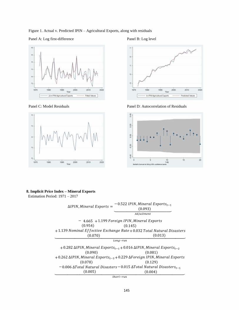
145
Figure 1. Actual v. Predicted IPIN – Agricultural Exports, along with residuals
Panel A: Log first-difference Panel B: Log level
Panel C: Model Residuals Panel D: Autocorrelation of Residuals
8. Implicit Price Index – Mineral Exports
Estimation Period: 1971 – 2017
∆𝐼𝑃𝐼𝑁,𝑀𝑖𝑛𝑒𝑟𝑎𝑙 𝐸𝑥𝑝𝑜𝑟𝑡𝑠 =−0.522 𝐼𝑃𝐼𝑁,𝑀𝑖𝑛𝑒𝑟𝑎𝑙 𝐸𝑥𝑝𝑜𝑟𝑡𝑠𝑡−1
(0.093)⏟ 𝐴𝑑𝑗𝑢𝑠𝑡𝑚𝑒𝑛𝑡
− 4.665(0.954)
+1.199 𝐹𝑜𝑟𝑒𝑖𝑔𝑛 𝐼𝑃𝐼𝑁,𝑀𝑖𝑛𝑒𝑟𝑎𝑙 𝐸𝑥𝑝𝑜𝑟𝑡𝑠
(0.145)
+1.139 𝑁𝑜𝑚𝑖𝑛𝑎𝑙 𝐸𝑓𝑓𝑒𝑐𝑡𝑖𝑣𝑒 𝐸𝑥𝑐ℎ𝑎𝑛𝑔𝑒 𝑅𝑎𝑡𝑒
(0.070)+0.032 𝑇𝑜𝑡𝑎𝑙 𝑁𝑎𝑡𝑢𝑟𝑎𝑙 𝐷𝑖𝑠𝑎𝑠𝑡𝑒𝑟𝑠
(0.013)⏟ 𝐿𝑜𝑛𝑔−𝑟𝑢𝑛
+0.282 ∆𝐼𝑃𝐼𝑁,𝑀𝑖𝑛𝑒𝑟𝑎𝑙 𝐸𝑥𝑝𝑜𝑟𝑡𝑠𝑡−1(0.090)
+0.016 ∆𝐼𝑃𝐼𝑁,𝑀𝑖𝑛𝑒𝑟𝑎𝑙 𝐸𝑥𝑝𝑜𝑟𝑡𝑠𝑡−2(0.081)
+0.262 ∆𝐼𝑃𝐼𝑁,𝑀𝑖𝑛𝑒𝑟𝑎𝑙 𝐸𝑥𝑝𝑜𝑟𝑡𝑠𝑡−3(0.078)
+0.229 ∆𝐹𝑜𝑟𝑒𝑖𝑔𝑛 𝐼𝑃𝐼𝑁,𝑀𝑖𝑛𝑒𝑟𝑎𝑙 𝐸𝑥𝑝𝑜𝑟𝑡𝑠
(0.129)−0.006 ∆𝑇𝑜𝑡𝑎𝑙 𝑁𝑎𝑡𝑢𝑟𝑎𝑙 𝐷𝑖𝑠𝑎𝑠𝑡𝑒𝑟𝑠
(0.005)−0.015 ∆𝑇𝑜𝑡𝑎𝑙 𝑁𝑎𝑡𝑢𝑟𝑎𝑙 𝐷𝑖𝑠𝑎𝑠𝑡𝑒𝑟𝑠𝑡−1
(0.004)⏟ 𝑆ℎ𝑜𝑟𝑡−𝑟𝑢𝑛

146
Table A1. Summary of model tests
Bounds Tests Hetoroskedasticity
Test Autocorrelation
Test Model Fit
F-Statistic t-statistic Breusch-Pagan Portmanteau Q-
Statistic MAE RMSE R2
χ2 (45) χ2 (21)
9.062 -5.574 1.848 17.007 0.079 0.110 0.767
[0.000, 0.001] [0.000, 0.001] [0.173] [0.710]
Figures in [] are p-values. Mean/SD/Min/Max of first-differenced (∆) IPIN – Mineral Exports are 0.084, 0.257, -
0.584, and 0.953 respectively.
Figure 1. Actual v. Predicted IPIN – Mineral Exports, along with residuals
Panel A: Log first-difference Panel B: Log level
Panel C: Model Residuals Panel D: Autocorrelation of Residuals
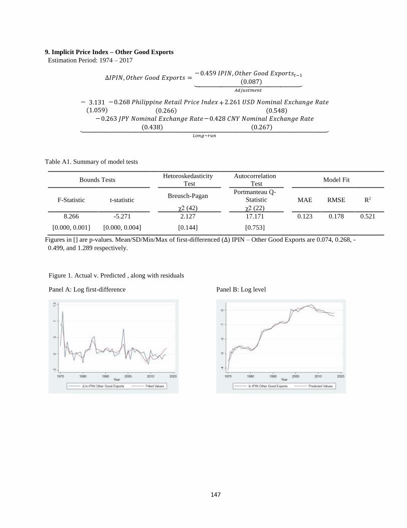
147
9. Implicit Price Index – Other Good Exports
Estimation Period: 1974 – 2017
∆𝐼𝑃𝐼𝑁, 𝑂𝑡ℎ𝑒𝑟 𝐺𝑜𝑜𝑑 𝐸𝑥𝑝𝑜𝑟𝑡𝑠 =−0.459 𝐼𝑃𝐼𝑁, 𝑂𝑡ℎ𝑒𝑟 𝐺𝑜𝑜𝑑 𝐸𝑥𝑝𝑜𝑟𝑡𝑠𝑡−1
(0.087)⏟ 𝐴𝑑𝑗𝑢𝑠𝑡𝑚𝑒𝑛𝑡
− 3.131(1.059)
−0.268 𝑃ℎ𝑖𝑙𝑖𝑝𝑝𝑖𝑛𝑒 𝑅𝑒𝑡𝑎𝑖𝑙 𝑃𝑟𝑖𝑐𝑒 𝐼𝑛𝑑𝑒𝑥
(0.266)+2.261 𝑈𝑆𝐷 𝑁𝑜𝑚𝑖𝑛𝑎𝑙 𝐸𝑥𝑐ℎ𝑎𝑛𝑔𝑒 𝑅𝑎𝑡𝑒
(0.548)−0.263 𝐽𝑃𝑌 𝑁𝑜𝑚𝑖𝑛𝑎𝑙 𝐸𝑥𝑐ℎ𝑎𝑛𝑔𝑒 𝑅𝑎𝑡𝑒
(0.438)
−0.428 𝐶𝑁𝑌 𝑁𝑜𝑚𝑖𝑛𝑎𝑙 𝐸𝑥𝑐ℎ𝑎𝑛𝑔𝑒 𝑅𝑎𝑡𝑒
(0.267)⏟ 𝐿𝑜𝑛𝑔−𝑟𝑢𝑛
Table A1. Summary of model tests
Bounds Tests Hetoroskedasticity
Test Autocorrelation
Test Model Fit
F-Statistic t-statistic Breusch-Pagan Portmanteau Q-
Statistic MAE RMSE R2
χ2 (42) χ2 (22)
8.266 -5.271 2.127 17.171 0.123 0.178 0.521
[0.000, 0.001] [0.000, 0.004] [0.144] [0.753]
Figures in [] are p-values. Mean/SD/Min/Max of first-differenced (∆) IPIN – Other Good Exports are 0.074, 0.268, -
0.499, and 1.289 respectively.
Figure 1. Actual v. Predicted , along with residuals
Panel A: Log first-difference Panel B: Log level
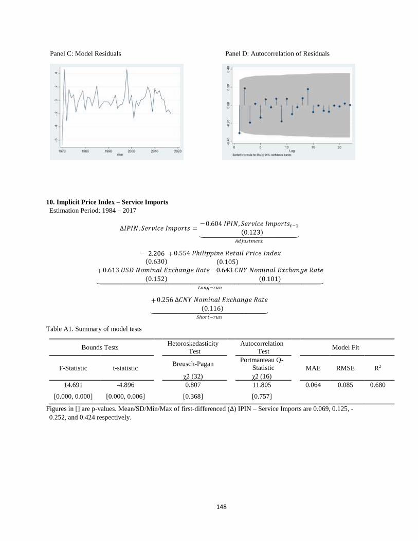
148
Panel C: Model Residuals Panel D: Autocorrelation of Residuals
10. Implicit Price Index – Service Imports
Estimation Period: 1984 – 2017
∆𝐼𝑃𝐼𝑁, 𝑆𝑒𝑟𝑣𝑖𝑐𝑒 𝐼𝑚𝑝𝑜𝑟𝑡𝑠 =−0.604 𝐼𝑃𝐼𝑁, 𝑆𝑒𝑟𝑣𝑖𝑐𝑒 𝐼𝑚𝑝𝑜𝑟𝑡𝑠𝑡−1
(0.123)⏟ 𝐴𝑑𝑗𝑢𝑠𝑡𝑚𝑒𝑛𝑡
− 2.206(0.630)
+0.554 𝑃ℎ𝑖𝑙𝑖𝑝𝑝𝑖𝑛𝑒 𝑅𝑒𝑡𝑎𝑖𝑙 𝑃𝑟𝑖𝑐𝑒 𝐼𝑛𝑑𝑒𝑥
(0.105)
+0.613 𝑈𝑆𝐷 𝑁𝑜𝑚𝑖𝑛𝑎𝑙 𝐸𝑥𝑐ℎ𝑎𝑛𝑔𝑒 𝑅𝑎𝑡𝑒
(0.152)
−0.643 𝐶𝑁𝑌 𝑁𝑜𝑚𝑖𝑛𝑎𝑙 𝐸𝑥𝑐ℎ𝑎𝑛𝑔𝑒 𝑅𝑎𝑡𝑒
(0.101)⏟ 𝐿𝑜𝑛𝑔−𝑟𝑢𝑛
+0.256 ∆𝐶𝑁𝑌 𝑁𝑜𝑚𝑖𝑛𝑎𝑙 𝐸𝑥𝑐ℎ𝑎𝑛𝑔𝑒 𝑅𝑎𝑡𝑒
(0.116)⏟ 𝑆ℎ𝑜𝑟𝑡−𝑟𝑢𝑛
Table A1. Summary of model tests
Bounds Tests Hetoroskedasticity
Test Autocorrelation
Test Model Fit
F-Statistic t-statistic Breusch-Pagan Portmanteau Q-
Statistic MAE RMSE R2
χ2 (32) χ2 (16)
14.691 -4.896 0.807 11.805 0.064 0.085 0.680
[0.000, 0.000] [0.000, 0.006] [0.368] [0.757]
Figures in [] are p-values. Mean/SD/Min/Max of first-differenced (∆) IPIN – Service Imports are 0.069, 0.125, -
0.252, and 0.424 respectively.

149
Figure 1. Actual v. Predicted IPIN – Service Imports, along with residuals
Panel A: Log first-difference Panel B: Log level
Panel C: Model Residuals Panel D: Autocorrelation of Residuals
11. Implicit Price Index – BPO Service Exports
Estimation Period: 1984 – 2017
∆𝐼𝑃𝐼𝑁, 𝐵𝑃𝑂 𝑆𝑒𝑟𝑣𝑖𝑐𝑒 𝐸𝑥𝑝𝑜𝑟𝑡𝑠 =−0.798 𝐼𝑃𝐼𝑁, 𝐵𝑃𝑂 𝑆𝑒𝑟𝑣𝑖𝑐𝑒 𝐸𝑥𝑝𝑜𝑟𝑡𝑠𝑡−1
(0.149)⏟ 𝐴𝑑𝑗𝑢𝑠𝑡𝑚𝑒𝑛𝑡
− 1.073(3.166)
+0.683 𝐹𝑜𝑟𝑒𝑖𝑔𝑛 𝐼𝑃𝐼𝑁, 𝐵𝑃𝑂 𝑆𝑒𝑟𝑣𝑖𝑐𝑒 𝐸𝑥𝑝𝑜𝑟𝑡𝑠
(0.182)+2.024 𝑈𝑆𝐷 𝑁𝑜𝑚𝑖𝑛𝑎𝑙 𝐸𝑥𝑐ℎ𝑎𝑛𝑔𝑒 𝑅𝑎𝑡𝑒
(0.732)
+1.713 𝐼𝑃𝐼𝑁,𝑀𝑎𝑡𝑒𝑟𝑖𝑎𝑙𝑠 𝐼𝑚𝑝𝑜𝑟𝑡𝑠(0.583)
+0.321 𝐼𝑃𝐼𝑁, 𝐹𝑢𝑒𝑙 𝐼𝑚𝑝𝑜𝑟𝑡𝑠(0.126)⏟
𝐿𝑜𝑛𝑔−𝑟𝑢𝑛
+0.239 ∆𝐼𝑃𝐼𝑁, 𝐵𝑃𝑂 𝑆𝑒𝑟𝑣𝑖𝑐𝑒 𝐸𝑥𝑝𝑜𝑟𝑡𝑠𝑡−1(0.150)
+0.364 ∆𝐼𝑃𝐼𝑁, 𝐵𝑃𝑂 𝑆𝑒𝑟𝑣𝑖𝑐𝑒 𝐸𝑥𝑝𝑜𝑟𝑡𝑠𝑡−2(0.156)
−0.307 ∆ 𝐼𝑃𝐼𝑁, 𝐹𝑢𝑒𝑙 𝐼𝑚𝑝𝑜𝑟𝑡𝑠(0.176)⏟
𝑆ℎ𝑜𝑟𝑡−𝑟𝑢𝑛
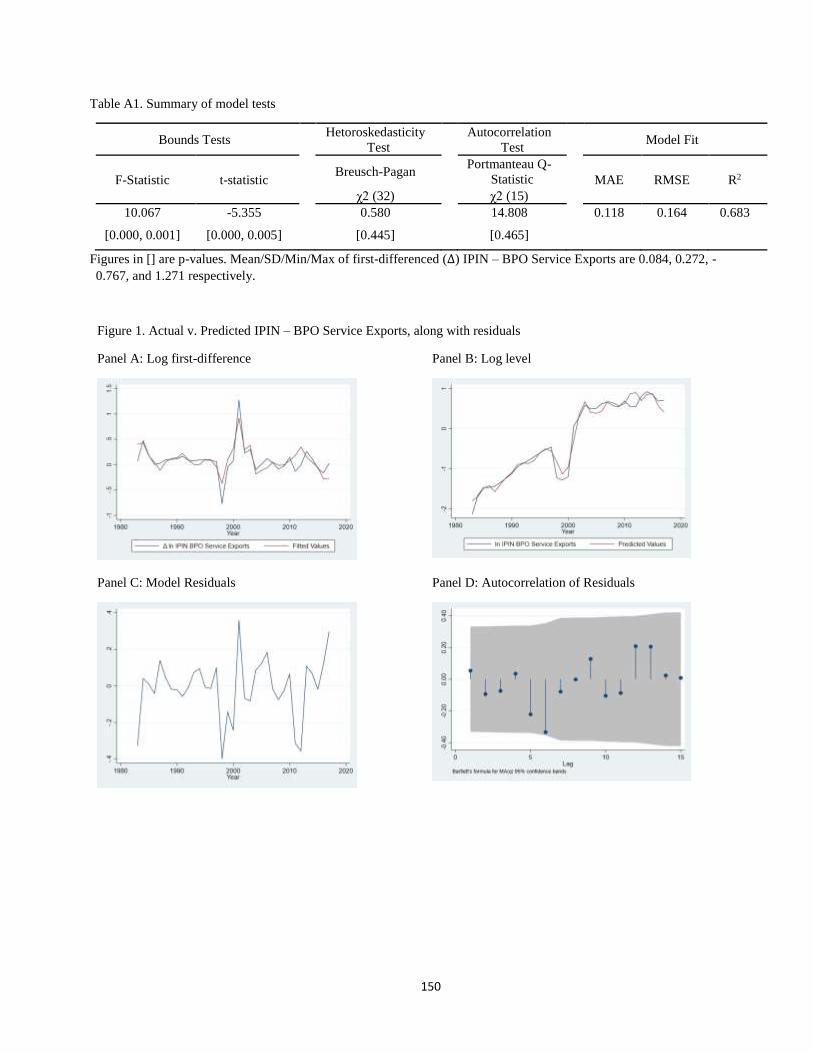
150
Table A1. Summary of model tests
Bounds Tests Hetoroskedasticity
Test Autocorrelation
Test Model Fit
F-Statistic t-statistic Breusch-Pagan Portmanteau Q-
Statistic MAE RMSE R2
χ2 (32) χ2 (15)
10.067 -5.355 0.580 14.808 0.118 0.164 0.683
[0.000, 0.001] [0.000, 0.005] [0.445] [0.465]
Figures in [] are p-values. Mean/SD/Min/Max of first-differenced (∆) IPIN – BPO Service Exports are 0.084, 0.272, -
0.767, and 1.271 respectively.
Figure 1. Actual v. Predicted IPIN – BPO Service Exports, along with residuals
Panel A: Log first-difference Panel B: Log level
Panel C: Model Residuals Panel D: Autocorrelation of Residuals

151
12. Implicit Price Index – Tourism Service Exports
Estimation Period: 1984 – 2017
∆𝐼𝑃𝐼𝑁, 𝑇𝑜𝑢𝑟𝑖𝑠𝑚 𝑆𝑒𝑟𝑣𝑖𝑐𝑒 𝐸𝑥𝑝𝑜𝑟𝑡𝑠 =−0.590 𝐼𝑃𝐼𝑁, 𝑇𝑜𝑢𝑟𝑖𝑠𝑚 𝑆𝑒𝑟𝑣𝑖𝑐𝑒 𝐸𝑥𝑝𝑜𝑟𝑡𝑠𝑡−1
(0.163)⏟ 𝐴𝑑𝑗𝑢𝑠𝑡𝑚𝑒𝑛𝑡
+ 2.650(4.616)
−1.338 𝐹𝑜𝑟𝑒𝑖𝑔𝑛 𝐼𝑃𝐼𝑁, 𝑇𝑜𝑢𝑟𝑖𝑠𝑚 𝑆𝑒𝑟𝑣𝑖𝑐𝑒 𝐸𝑥𝑝𝑜𝑟𝑡𝑠
(0.042)−0.407 𝑁𝑜𝑚𝑖𝑛𝑎𝑙 𝐸𝑓𝑓𝑒𝑐𝑡𝑖𝑣𝑒 𝐸𝑥𝑐ℎ𝑎𝑛𝑔𝑒 𝑅𝑎𝑡𝑒
(0.401)+2.939 𝑃ℎ𝑖𝑙𝑖𝑝𝑝𝑖𝑛𝑒 𝑊ℎ𝑜𝑙𝑒𝑠𝑎𝑙𝑒 𝑃𝑟𝑖𝑐𝑒 𝐼𝑛𝑑𝑒𝑥
(0.248)⏟ 𝐿𝑜𝑛𝑔−𝑟𝑢𝑛
Table A1. Summary of model tests
Bounds Tests Hetoroskedasticity
Test Autocorrelation
Test Model Fit
F-Statistic t-statistic Breusch-Pagan Portmanteau Q-
Statistic MAE RMSE R2
χ2 (32) χ2 (16)
4.113 -3.616 1.236 14.355 0.206 0.310 0.362
[0.030, 0.098] [0.011, 0.078] [0.266] [0.572]
Figures in [] are p-values. Mean/SD/Min/Max of first-differenced (∆) IPIN – Tourism Service Exports are 0.084,
0.0342, -0.900, and 1.256 respectively.
Figure 1. Actual v. Predicted IPIN – Tourism Service Exports, along with residuals
Panel A: Log first-difference Panel B: Log level
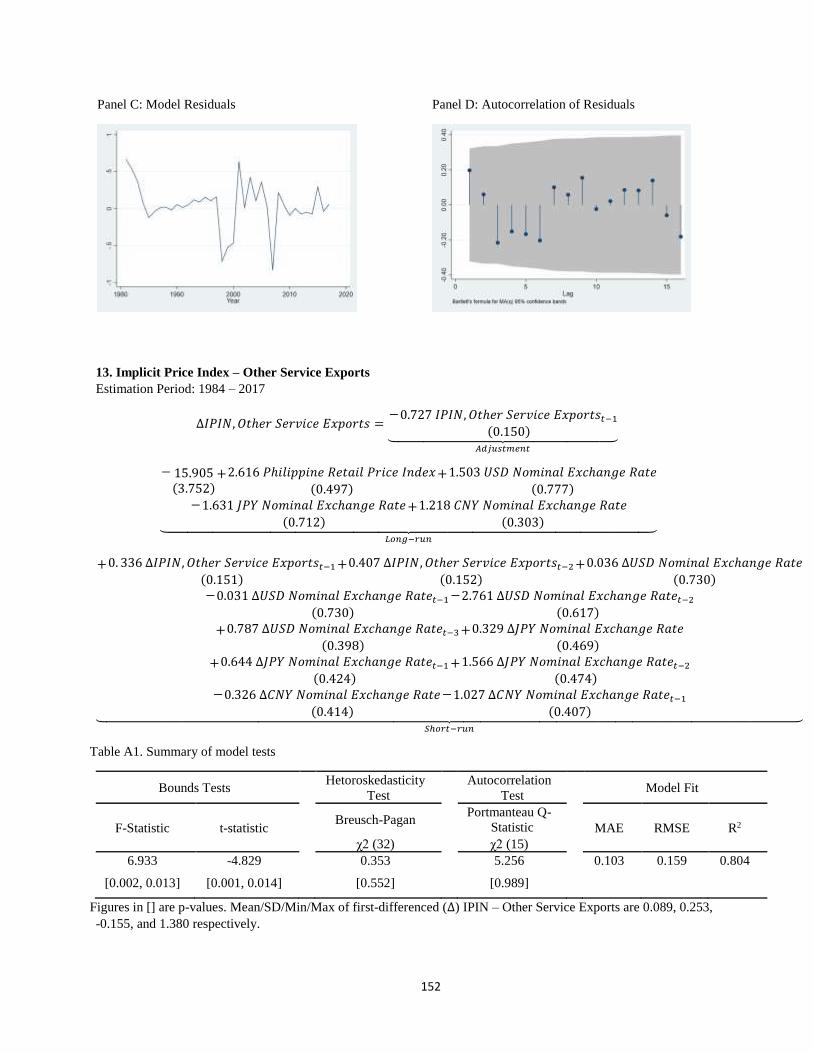
152
Panel C: Model Residuals Panel D: Autocorrelation of Residuals
13. Implicit Price Index – Other Service Exports
Estimation Period: 1984 – 2017
∆𝐼𝑃𝐼𝑁, 𝑂𝑡ℎ𝑒𝑟 𝑆𝑒𝑟𝑣𝑖𝑐𝑒 𝐸𝑥𝑝𝑜𝑟𝑡𝑠 =−0.727 𝐼𝑃𝐼𝑁, 𝑂𝑡ℎ𝑒𝑟 𝑆𝑒𝑟𝑣𝑖𝑐𝑒 𝐸𝑥𝑝𝑜𝑟𝑡𝑠𝑡−1
(0.150)⏟ 𝐴𝑑𝑗𝑢𝑠𝑡𝑚𝑒𝑛𝑡
− 15.905(3.752)
+2.616 𝑃ℎ𝑖𝑙𝑖𝑝𝑝𝑖𝑛𝑒 𝑅𝑒𝑡𝑎𝑖𝑙 𝑃𝑟𝑖𝑐𝑒 𝐼𝑛𝑑𝑒𝑥
(0.497)+1.503 𝑈𝑆𝐷 𝑁𝑜𝑚𝑖𝑛𝑎𝑙 𝐸𝑥𝑐ℎ𝑎𝑛𝑔𝑒 𝑅𝑎𝑡𝑒
(0.777)−1.631 𝐽𝑃𝑌 𝑁𝑜𝑚𝑖𝑛𝑎𝑙 𝐸𝑥𝑐ℎ𝑎𝑛𝑔𝑒 𝑅𝑎𝑡𝑒
(0.712)+1.218 𝐶𝑁𝑌 𝑁𝑜𝑚𝑖𝑛𝑎𝑙 𝐸𝑥𝑐ℎ𝑎𝑛𝑔𝑒 𝑅𝑎𝑡𝑒
(0.303)⏟ 𝐿𝑜𝑛𝑔−𝑟𝑢𝑛
+0. 336 ∆𝐼𝑃𝐼𝑁, 𝑂𝑡ℎ𝑒𝑟 𝑆𝑒𝑟𝑣𝑖𝑐𝑒 𝐸𝑥𝑝𝑜𝑟𝑡𝑠𝑡−1(0.151)
+0.407 ∆𝐼𝑃𝐼𝑁, 𝑂𝑡ℎ𝑒𝑟 𝑆𝑒𝑟𝑣𝑖𝑐𝑒 𝐸𝑥𝑝𝑜𝑟𝑡𝑠𝑡−2(0.152)
+0.036 ∆𝑈𝑆𝐷 𝑁𝑜𝑚𝑖𝑛𝑎𝑙 𝐸𝑥𝑐ℎ𝑎𝑛𝑔𝑒 𝑅𝑎𝑡𝑒
(0.730)−0.031 ∆𝑈𝑆𝐷 𝑁𝑜𝑚𝑖𝑛𝑎𝑙 𝐸𝑥𝑐ℎ𝑎𝑛𝑔𝑒 𝑅𝑎𝑡𝑒𝑡−1
(0.730)
−2.761 ∆𝑈𝑆𝐷 𝑁𝑜𝑚𝑖𝑛𝑎𝑙 𝐸𝑥𝑐ℎ𝑎𝑛𝑔𝑒 𝑅𝑎𝑡𝑒𝑡−2(0.617)
+0.787 ∆𝑈𝑆𝐷 𝑁𝑜𝑚𝑖𝑛𝑎𝑙 𝐸𝑥𝑐ℎ𝑎𝑛𝑔𝑒 𝑅𝑎𝑡𝑒𝑡−3(0.398)
+0.329 ∆𝐽𝑃𝑌 𝑁𝑜𝑚𝑖𝑛𝑎𝑙 𝐸𝑥𝑐ℎ𝑎𝑛𝑔𝑒 𝑅𝑎𝑡𝑒
(0.469)
+0.644 ∆𝐽𝑃𝑌 𝑁𝑜𝑚𝑖𝑛𝑎𝑙 𝐸𝑥𝑐ℎ𝑎𝑛𝑔𝑒 𝑅𝑎𝑡𝑒𝑡−1(0.424)
+1.566 ∆𝐽𝑃𝑌 𝑁𝑜𝑚𝑖𝑛𝑎𝑙 𝐸𝑥𝑐ℎ𝑎𝑛𝑔𝑒 𝑅𝑎𝑡𝑒𝑡−2(0.474)
−0.326 ∆𝐶𝑁𝑌 𝑁𝑜𝑚𝑖𝑛𝑎𝑙 𝐸𝑥𝑐ℎ𝑎𝑛𝑔𝑒 𝑅𝑎𝑡𝑒
(0.414)
−1.027 ∆𝐶𝑁𝑌 𝑁𝑜𝑚𝑖𝑛𝑎𝑙 𝐸𝑥𝑐ℎ𝑎𝑛𝑔𝑒 𝑅𝑎𝑡𝑒𝑡−1(0.407)⏟
𝑆ℎ𝑜𝑟𝑡−𝑟𝑢𝑛
Table A1. Summary of model tests
Bounds Tests Hetoroskedasticity
Test Autocorrelation
Test Model Fit
F-Statistic t-statistic Breusch-Pagan Portmanteau Q-
Statistic MAE RMSE R2
χ2 (32) χ2 (15)
6.933 -4.829 0.353 5.256 0.103 0.159 0.804
[0.002, 0.013] [0.001, 0.014] [0.552] [0.989]
Figures in [] are p-values. Mean/SD/Min/Max of first-differenced (∆) IPIN – Other Service Exports are 0.089, 0.253,
-0.155, and 1.380 respectively.
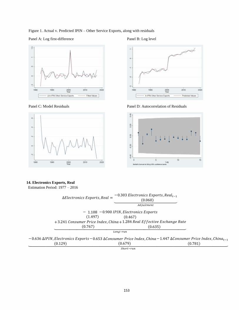
153
Figure 1. Actual v. Predicted IPIN – Other Service Exports, along with residuals
Panel A: Log first-difference Panel B: Log level
Panel C: Model Residuals Panel D: Autocorrelation of Residuals
14. Electronics Exports, Real
Estimation Period: 1977 – 2016
∆𝐸𝑙𝑒𝑐𝑡𝑟𝑜𝑛𝑖𝑐𝑠 𝐸𝑥𝑝𝑜𝑟𝑡𝑠, 𝑅𝑒𝑎𝑙 =−0.303 𝐸𝑙𝑒𝑐𝑡𝑟𝑜𝑛𝑖𝑐𝑠 𝐸𝑥𝑝𝑜𝑟𝑡𝑠, 𝑅𝑒𝑎𝑙𝑡−1
(0.060)⏟ 𝐴𝑑𝑗𝑢𝑠𝑡𝑚𝑒𝑛𝑡
− 1.108(1.497)
−0.900 𝐼𝑃𝐼𝑁, 𝐸𝑙𝑒𝑐𝑡𝑟𝑜𝑛𝑖𝑐𝑠 𝐸𝑥𝑝𝑜𝑟𝑡𝑠
(0.467)
+3.241 𝐶𝑜𝑛𝑠𝑢𝑚𝑒𝑟 𝑃𝑟𝑖𝑐𝑒 𝐼𝑛𝑑𝑒𝑥, 𝐶ℎ𝑖𝑛𝑎(0.767)
+1.284 𝑅𝑒𝑎𝑙 𝐸𝑓𝑓𝑒𝑐𝑡𝑖𝑣𝑒 𝐸𝑥𝑐ℎ𝑎𝑛𝑔𝑒 𝑅𝑎𝑡𝑒
(0.635)⏟ 𝐿𝑜𝑛𝑔−𝑟𝑢𝑛
−0.636 ∆𝐼𝑃𝐼𝑁, 𝐸𝑙𝑒𝑐𝑡𝑟𝑜𝑛𝑖𝑐𝑠 𝐸𝑥𝑝𝑜𝑟𝑡𝑠(0.129)
−0.653 ∆𝐶𝑜𝑛𝑠𝑢𝑚𝑒𝑟 𝑃𝑟𝑖𝑐𝑒 𝐼𝑛𝑑𝑒𝑥, 𝐶ℎ𝑖𝑛𝑎(0.679)
−1.447 ∆𝐶𝑜𝑛𝑠𝑢𝑚𝑒𝑟 𝑃𝑟𝑖𝑐𝑒 𝐼𝑛𝑑𝑒𝑥, 𝐶ℎ𝑖𝑛𝑎𝑡−1(0.781)⏟
𝑆ℎ𝑜𝑟𝑡−𝑟𝑢𝑛
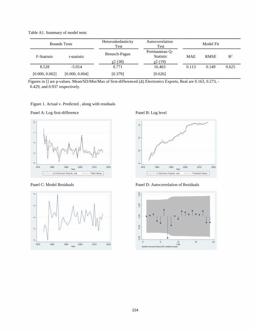
154
Table A1. Summary of model tests
Bounds Tests Hetoroskedasticity
Test Autocorrelation
Test Model Fit
F-Statistic t-statistic Breusch-Pagan Portmanteau Q-
Statistic MAE RMSE R2
χ2 (38) χ2 (19)
8.528 -5.014 0.771 16.463 0.113 0.149 0.625
[0.000, 0.002] [0.000, 0.004] [0.379] [0.626]
Figures in [] are p-values. Mean/SD/Min/Max of first-differenced (∆) Electronics Exports, Real are 0.163, 0.273, -
0.429, and 0.937 respectively.
Figure 1. Actual v. Predicted , along with residuals
Panel A: Log first-difference Panel B: Log level
Panel C: Model Residuals Panel D: Autocorrelation of Residuals
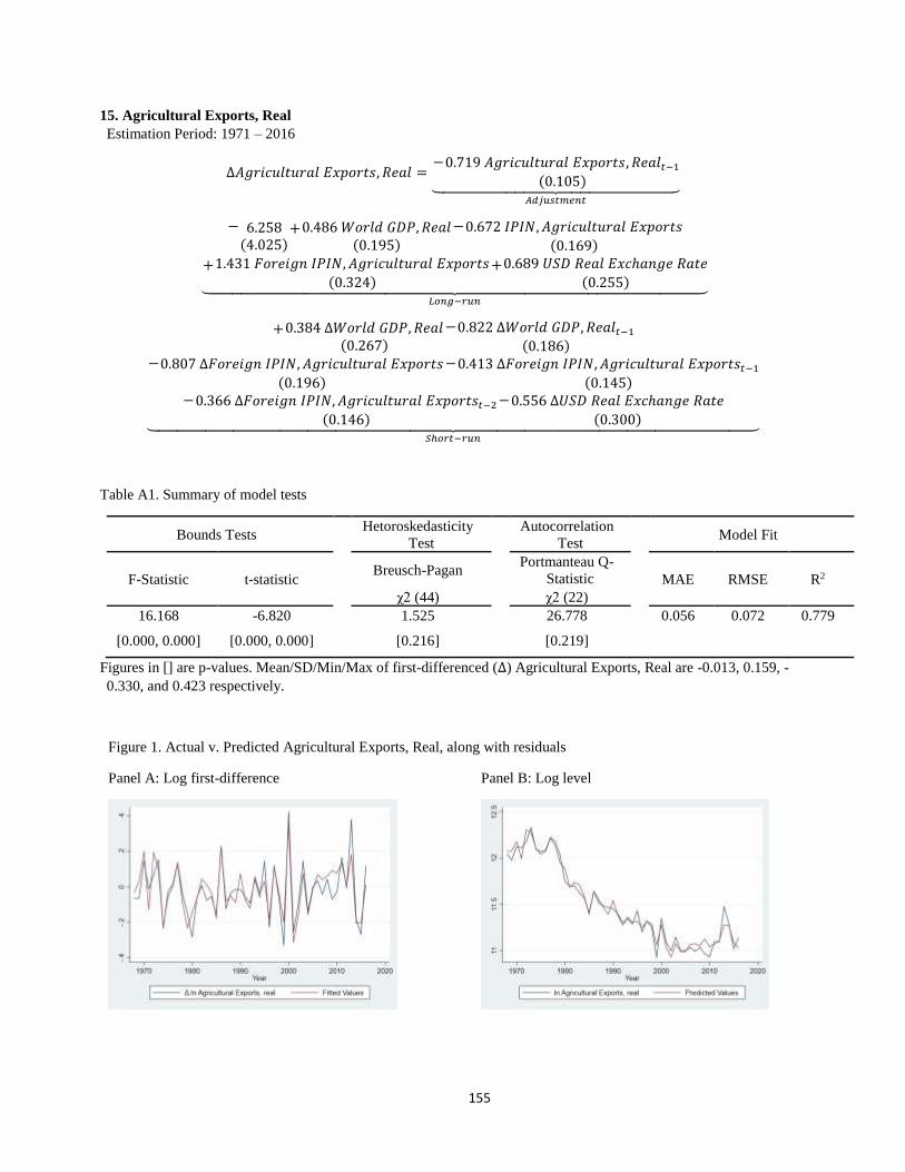
155
15. Agricultural Exports, Real
Estimation Period: 1971 – 2016
∆𝐴𝑔𝑟𝑖𝑐𝑢𝑙𝑡𝑢𝑟𝑎𝑙 𝐸𝑥𝑝𝑜𝑟𝑡𝑠, 𝑅𝑒𝑎𝑙 =−0.719 𝐴𝑔𝑟𝑖𝑐𝑢𝑙𝑡𝑢𝑟𝑎𝑙 𝐸𝑥𝑝𝑜𝑟𝑡𝑠, 𝑅𝑒𝑎𝑙𝑡−1
(0.105)⏟ 𝐴𝑑𝑗𝑢𝑠𝑡𝑚𝑒𝑛𝑡
− 6.258(4.025)
+0.486 𝑊𝑜𝑟𝑙𝑑 𝐺𝐷𝑃, 𝑅𝑒𝑎𝑙(0.195)
−0.672 𝐼𝑃𝐼𝑁, 𝐴𝑔𝑟𝑖𝑐𝑢𝑙𝑡𝑢𝑟𝑎𝑙 𝐸𝑥𝑝𝑜𝑟𝑡𝑠
(0.169)
+1.431 𝐹𝑜𝑟𝑒𝑖𝑔𝑛 𝐼𝑃𝐼𝑁, 𝐴𝑔𝑟𝑖𝑐𝑢𝑙𝑡𝑢𝑟𝑎𝑙 𝐸𝑥𝑝𝑜𝑟𝑡𝑠
(0.324)+0.689 𝑈𝑆𝐷 𝑅𝑒𝑎𝑙 𝐸𝑥𝑐ℎ𝑎𝑛𝑔𝑒 𝑅𝑎𝑡𝑒
(0.255)⏟ 𝐿𝑜𝑛𝑔−𝑟𝑢𝑛
+0.384 ∆𝑊𝑜𝑟𝑙𝑑 𝐺𝐷𝑃, 𝑅𝑒𝑎𝑙(0.267)
−0.822 ∆𝑊𝑜𝑟𝑙𝑑 𝐺𝐷𝑃, 𝑅𝑒𝑎𝑙𝑡−1(0.186)
−0.807 ∆𝐹𝑜𝑟𝑒𝑖𝑔𝑛 𝐼𝑃𝐼𝑁, 𝐴𝑔𝑟𝑖𝑐𝑢𝑙𝑡𝑢𝑟𝑎𝑙 𝐸𝑥𝑝𝑜𝑟𝑡𝑠
(0.196)
−0.413 ∆𝐹𝑜𝑟𝑒𝑖𝑔𝑛 𝐼𝑃𝐼𝑁, 𝐴𝑔𝑟𝑖𝑐𝑢𝑙𝑡𝑢𝑟𝑎𝑙 𝐸𝑥𝑝𝑜𝑟𝑡𝑠𝑡−1(0.145)
−0.366 ∆𝐹𝑜𝑟𝑒𝑖𝑔𝑛 𝐼𝑃𝐼𝑁, 𝐴𝑔𝑟𝑖𝑐𝑢𝑙𝑡𝑢𝑟𝑎𝑙 𝐸𝑥𝑝𝑜𝑟𝑡𝑠𝑡−2(0.146)
−0.556 ∆𝑈𝑆𝐷 𝑅𝑒𝑎𝑙 𝐸𝑥𝑐ℎ𝑎𝑛𝑔𝑒 𝑅𝑎𝑡𝑒
(0.300)⏟ 𝑆ℎ𝑜𝑟𝑡−𝑟𝑢𝑛
Table A1. Summary of model tests
Bounds Tests Hetoroskedasticity
Test Autocorrelation
Test Model Fit
F-Statistic t-statistic Breusch-Pagan Portmanteau Q-
Statistic MAE RMSE R2
χ2 (44) χ2 (22)
16.168 -6.820 1.525 26.778 0.056 0.072 0.779
[0.000, 0.000] [0.000, 0.000] [0.216] [0.219]
Figures in [] are p-values. Mean/SD/Min/Max of first-differenced (∆) Agricultural Exports, Real are -0.013, 0.159, -
0.330, and 0.423 respectively.
Figure 1. Actual v. Predicted Agricultural Exports, Real, along with residuals
Panel A: Log first-difference Panel B: Log level
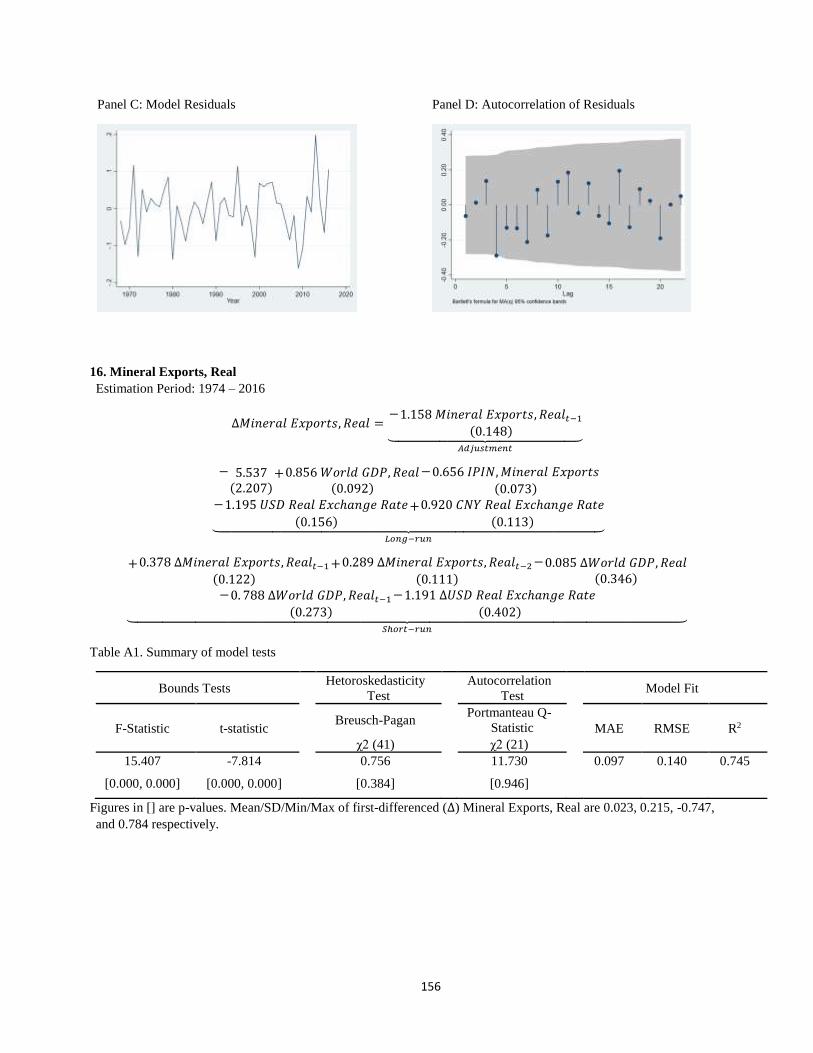
156
Panel C: Model Residuals Panel D: Autocorrelation of Residuals
16. Mineral Exports, Real
Estimation Period: 1974 – 2016
∆𝑀𝑖𝑛𝑒𝑟𝑎𝑙 𝐸𝑥𝑝𝑜𝑟𝑡𝑠, 𝑅𝑒𝑎𝑙 =−1.158 𝑀𝑖𝑛𝑒𝑟𝑎𝑙 𝐸𝑥𝑝𝑜𝑟𝑡𝑠, 𝑅𝑒𝑎𝑙𝑡−1
(0.148)⏟ 𝐴𝑑𝑗𝑢𝑠𝑡𝑚𝑒𝑛𝑡
− 5.537(2.207)
+0.856 𝑊𝑜𝑟𝑙𝑑 𝐺𝐷𝑃, 𝑅𝑒𝑎𝑙(0.092)
−0.656 𝐼𝑃𝐼𝑁,𝑀𝑖𝑛𝑒𝑟𝑎𝑙 𝐸𝑥𝑝𝑜𝑟𝑡𝑠
(0.073)−1.195 𝑈𝑆𝐷 𝑅𝑒𝑎𝑙 𝐸𝑥𝑐ℎ𝑎𝑛𝑔𝑒 𝑅𝑎𝑡𝑒
(0.156)+0.920 𝐶𝑁𝑌 𝑅𝑒𝑎𝑙 𝐸𝑥𝑐ℎ𝑎𝑛𝑔𝑒 𝑅𝑎𝑡𝑒
(0.113)⏟ 𝐿𝑜𝑛𝑔−𝑟𝑢𝑛
+0.378 ∆𝑀𝑖𝑛𝑒𝑟𝑎𝑙 𝐸𝑥𝑝𝑜𝑟𝑡𝑠, 𝑅𝑒𝑎𝑙𝑡−1(0.122)
+0.289 ∆𝑀𝑖𝑛𝑒𝑟𝑎𝑙 𝐸𝑥𝑝𝑜𝑟𝑡𝑠, 𝑅𝑒𝑎𝑙𝑡−2(0.111)
−0.085 ∆𝑊𝑜𝑟𝑙𝑑 𝐺𝐷𝑃, 𝑅𝑒𝑎𝑙(0.346)
−0. 788 ∆𝑊𝑜𝑟𝑙𝑑 𝐺𝐷𝑃, 𝑅𝑒𝑎𝑙𝑡−1(0.273)
−1.191 ∆𝑈𝑆𝐷 𝑅𝑒𝑎𝑙 𝐸𝑥𝑐ℎ𝑎𝑛𝑔𝑒 𝑅𝑎𝑡𝑒
(0.402)⏟ 𝑆ℎ𝑜𝑟𝑡−𝑟𝑢𝑛
Table A1. Summary of model tests
Bounds Tests Hetoroskedasticity
Test Autocorrelation
Test Model Fit
F-Statistic t-statistic Breusch-Pagan Portmanteau Q-
Statistic MAE RMSE R2
χ2 (41) χ2 (21)
15.407 -7.814 0.756 11.730 0.097 0.140 0.745
[0.000, 0.000] [0.000, 0.000] [0.384] [0.946]
Figures in [] are p-values. Mean/SD/Min/Max of first-differenced (∆) Mineral Exports, Real are 0.023, 0.215, -0.747,
and 0.784 respectively.

157
Figure 1. Actual v. Predicted Mineral Exports, Real, along with residuals
Panel A: Log first-difference Panel B: Log level
Panel C: Model Residuals Panel D: Autocorrelation of Residuals
17. Other Good Exports, Real
Estimation Period: 1973 – 2016
∆𝑂𝑡ℎ𝑒𝑟 𝐺𝑜𝑜𝑑 𝐸𝑥𝑝𝑜𝑟𝑡𝑠, 𝑅𝑒𝑎𝑙 =−0.879 𝑂𝑡ℎ𝑒𝑟 𝐺𝑜𝑜𝑑 𝐸𝑥𝑝𝑜𝑟𝑡𝑠, 𝑅𝑒𝑎𝑙𝑡−1
(0.139)⏟ 𝐴𝑑𝑗𝑢𝑠𝑡𝑚𝑒𝑛𝑡
− 0.054(2.149)
+1.008 𝑊𝑜𝑟𝑙𝑑 𝐺𝐷𝑃, 𝑅𝑒𝑎𝑙(0.085)
−0.568 𝐼𝑃𝐼𝑁, 𝑂𝑡ℎ𝑒𝑟 𝐺𝑜𝑜𝑑 𝐸𝑥𝑝𝑜𝑟𝑡𝑠
(0.085)−2.053 𝑈𝑆𝐷 𝑅𝑒𝑎𝑙 𝐸𝑥𝑐ℎ𝑎𝑛𝑔𝑒 𝑅𝑎𝑡𝑒
(0.255)+0.519 𝐽𝑃𝑌 𝑅𝑒𝑎𝑙 𝐸𝑥𝑐ℎ𝑎𝑛𝑔𝑒 𝑅𝑎𝑡𝑒
(0.139)⏟ 𝐿𝑜𝑛𝑔−𝑟𝑢𝑛
+0. 263 ∆𝑂𝑡ℎ𝑒𝑟 𝐺𝑜𝑜𝑑 𝐸𝑥𝑝𝑜𝑟𝑡𝑠, 𝑅𝑒𝑎𝑙𝑡−1(0.133)
+0.009 ∆𝑊𝑜𝑟𝑙𝑑 𝐺𝐷𝑃, 𝑅𝑒𝑎𝑙(0.361)
−0.869 ∆𝑊𝑜𝑟𝑙𝑑 𝐺𝐷𝑃, 𝑅𝑒𝑎𝑙𝑡−1(0.339)
−0.239 ∆𝐼𝑃𝐼𝑁, 𝑂𝑡ℎ𝑒𝑟 𝐺𝑜𝑜𝑑 𝐸𝑥𝑝𝑜𝑟𝑡𝑠(0.131)
+0.087 ∆𝐼𝑃𝐼𝑁, 𝑂𝑡ℎ𝑒𝑟 𝐺𝑜𝑜𝑑 𝐸𝑥𝑝𝑜𝑟𝑡𝑠𝑡−1(0.131)
+0.294 ∆𝐼𝑃𝐼𝑁, 𝑂𝑡ℎ𝑒𝑟 𝐺𝑜𝑜𝑑 𝐸𝑥𝑝𝑜𝑟𝑡𝑠𝑡−2(0.074)
+1.020 ∆𝑈𝑆𝐷 𝑅𝑒𝑎𝑙 𝐸𝑥𝑐ℎ𝑎𝑛𝑔𝑒 𝑅𝑎𝑡𝑒
(0.441)+1.620 ∆𝑈𝑆𝐷 𝑅𝑒𝑎𝑙 𝐸𝑥𝑐ℎ𝑎𝑛𝑔𝑒 𝑅𝑎𝑡𝑒𝑡−1
(0.403)+1.305 ∆𝑈𝑆𝐷 𝑅𝑒𝑎𝑙 𝐸𝑥𝑐ℎ𝑎𝑛𝑔𝑒 𝑅𝑎𝑡𝑒𝑡−2
(0.325)−0.438 ∆𝐽𝑃𝑌 𝑅𝑒𝑎𝑙 𝐸𝑥𝑐ℎ𝑎𝑛𝑔𝑒 𝑅𝑎𝑡𝑒
(0.223)
−0.463 ∆𝐽𝑃𝑌 𝑅𝑒𝑎𝑙 𝐸𝑥𝑐ℎ𝑎𝑛𝑔𝑒 𝑅𝑎𝑡𝑒𝑡−1(0.213)
−0.389 ∆𝐽𝑃𝑌 𝑅𝑒𝑎𝑙 𝐸𝑥𝑐ℎ𝑎𝑛𝑔𝑒 𝑅𝑎𝑡𝑒𝑡−2(0.195)⏟
𝑆ℎ𝑜𝑟𝑡−𝑟𝑢𝑛
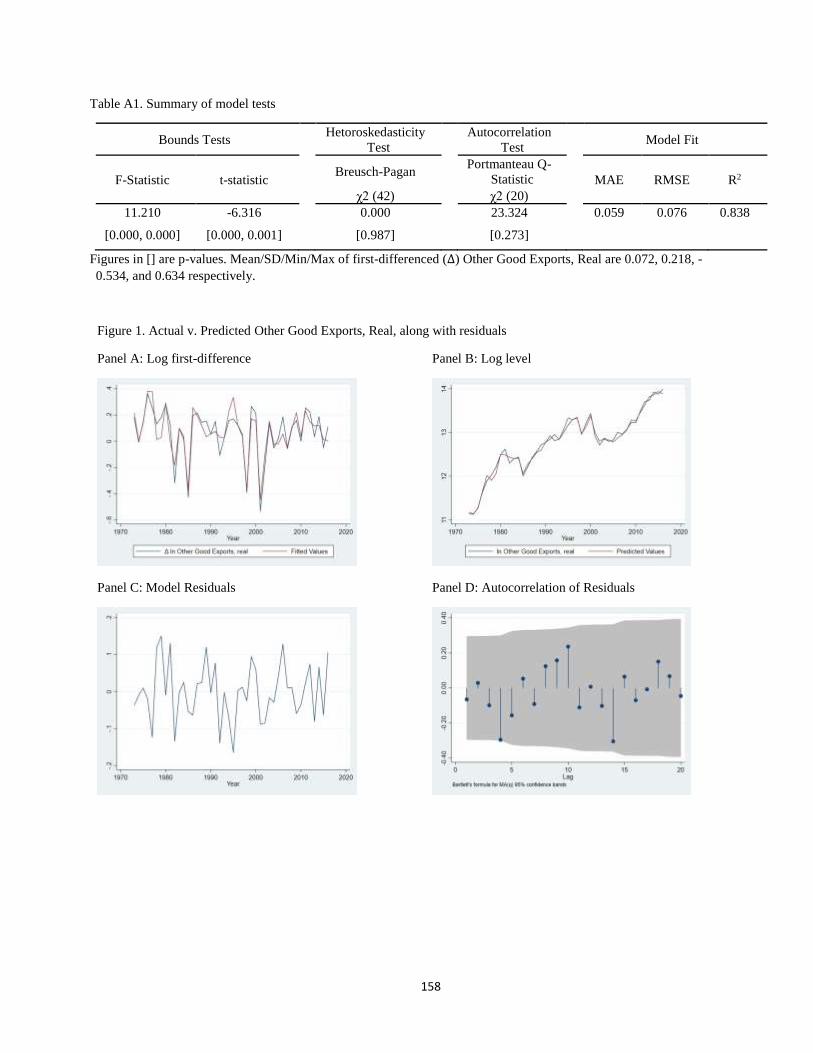
158
Table A1. Summary of model tests
Bounds Tests Hetoroskedasticity
Test Autocorrelation
Test Model Fit
F-Statistic t-statistic Breusch-Pagan Portmanteau Q-
Statistic MAE RMSE R2
χ2 (42) χ2 (20)
11.210 -6.316 0.000 23.324 0.059 0.076 0.838
[0.000, 0.000] [0.000, 0.001] [0.987] [0.273]
Figures in [] are p-values. Mean/SD/Min/Max of first-differenced (∆) Other Good Exports, Real are 0.072, 0.218, -
0.534, and 0.634 respectively.
Figure 1. Actual v. Predicted Other Good Exports, Real, along with residuals
Panel A: Log first-difference Panel B: Log level
Panel C: Model Residuals Panel D: Autocorrelation of Residuals
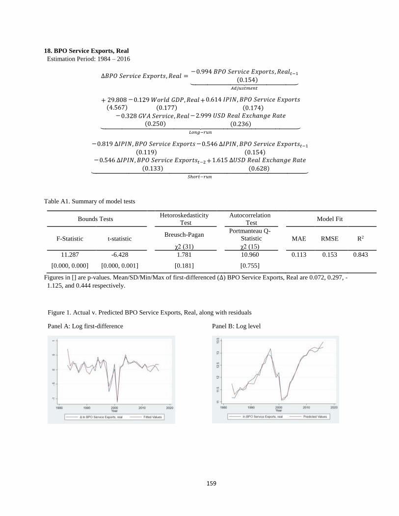
159
18. BPO Service Exports, Real
Estimation Period: 1984 – 2016
∆𝐵𝑃𝑂 𝑆𝑒𝑟𝑣𝑖𝑐𝑒 𝐸𝑥𝑝𝑜𝑟𝑡𝑠, 𝑅𝑒𝑎𝑙 =−0.994 𝐵𝑃𝑂 𝑆𝑒𝑟𝑣𝑖𝑐𝑒 𝐸𝑥𝑝𝑜𝑟𝑡𝑠, 𝑅𝑒𝑎𝑙𝑡−1
(0.154)⏟ 𝐴𝑑𝑗𝑢𝑠𝑡𝑚𝑒𝑛𝑡
+ 29.808(4.567)
−0.129 𝑊𝑜𝑟𝑙𝑑 𝐺𝐷𝑃,𝑅𝑒𝑎𝑙(0.177)
+0.614 𝐼𝑃𝐼𝑁, 𝐵𝑃𝑂 𝑆𝑒𝑟𝑣𝑖𝑐𝑒 𝐸𝑥𝑝𝑜𝑟𝑡𝑠
(0.174)−0.328 𝐺𝑉𝐴 𝑆𝑒𝑟𝑣𝑖𝑐𝑒, 𝑅𝑒𝑎𝑙
(0.250)
−2.999 𝑈𝑆𝐷 𝑅𝑒𝑎𝑙 𝐸𝑥𝑐ℎ𝑎𝑛𝑔𝑒 𝑅𝑎𝑡𝑒
(0.236)⏟ 𝐿𝑜𝑛𝑔−𝑟𝑢𝑛
−0.819 ∆𝐼𝑃𝐼𝑁, 𝐵𝑃𝑂 𝑆𝑒𝑟𝑣𝑖𝑐𝑒 𝐸𝑥𝑝𝑜𝑟𝑡𝑠
(0.119)
−0.546 ∆𝐼𝑃𝐼𝑁, 𝐵𝑃𝑂 𝑆𝑒𝑟𝑣𝑖𝑐𝑒 𝐸𝑥𝑝𝑜𝑟𝑡𝑠𝑡−1(0.154)
−0.546 ∆𝐼𝑃𝐼𝑁, 𝐵𝑃𝑂 𝑆𝑒𝑟𝑣𝑖𝑐𝑒 𝐸𝑥𝑝𝑜𝑟𝑡𝑠𝑡−2(0.133)
+1.615 ∆𝑈𝑆𝐷 𝑅𝑒𝑎𝑙 𝐸𝑥𝑐ℎ𝑎𝑛𝑔𝑒 𝑅𝑎𝑡𝑒
(0.628)⏟ 𝑆ℎ𝑜𝑟𝑡−𝑟𝑢𝑛
Table A1. Summary of model tests
Bounds Tests Hetoroskedasticity
Test Autocorrelation
Test Model Fit
F-Statistic t-statistic Breusch-Pagan Portmanteau Q-
Statistic MAE RMSE R2
χ2 (31) χ2 (15)
11.287 -6.428 1.781 10.960 0.113 0.153 0.843
[0.000, 0.000] [0.000, 0.001] [0.181] [0.755]
Figures in [] are p-values. Mean/SD/Min/Max of first-differenced (∆) BPO Service Exports, Real are 0.072, 0.297, -
1.125, and 0.444 respectively.
Figure 1. Actual v. Predicted BPO Service Exports, Real, along with residuals
Panel A: Log first-difference Panel B: Log level
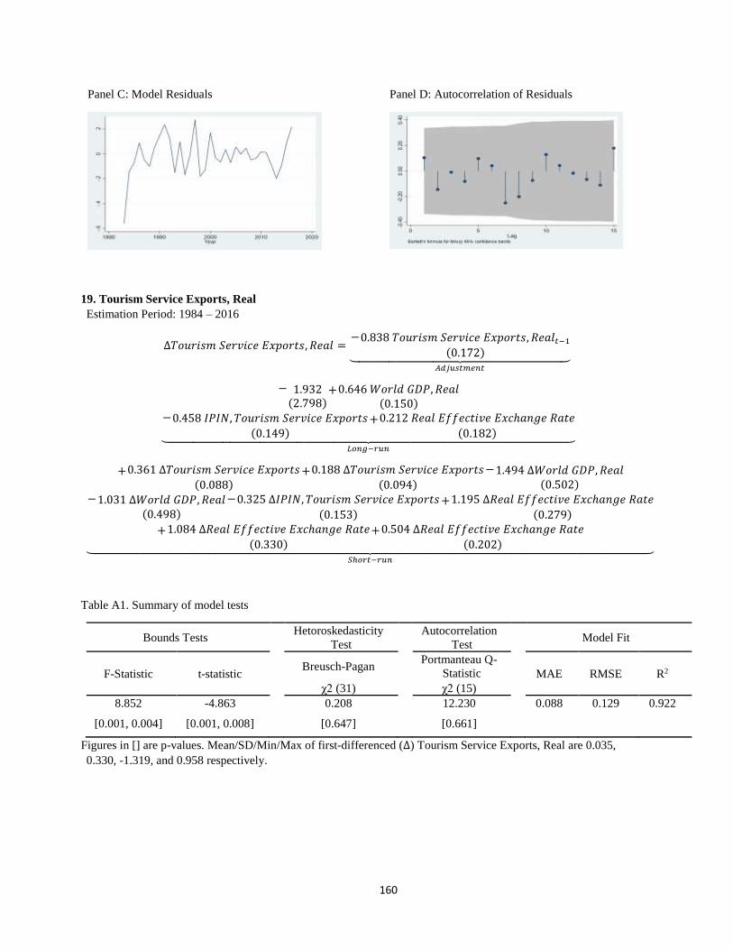
160
Panel C: Model Residuals Panel D: Autocorrelation of Residuals
19. Tourism Service Exports, Real
Estimation Period: 1984 – 2016
∆𝑇𝑜𝑢𝑟𝑖𝑠𝑚 𝑆𝑒𝑟𝑣𝑖𝑐𝑒 𝐸𝑥𝑝𝑜𝑟𝑡𝑠, 𝑅𝑒𝑎𝑙 =−0.838 𝑇𝑜𝑢𝑟𝑖𝑠𝑚 𝑆𝑒𝑟𝑣𝑖𝑐𝑒 𝐸𝑥𝑝𝑜𝑟𝑡𝑠, 𝑅𝑒𝑎𝑙𝑡−1
(0.172)⏟ 𝐴𝑑𝑗𝑢𝑠𝑡𝑚𝑒𝑛𝑡
− 1.932(2.798)
+0.646 𝑊𝑜𝑟𝑙𝑑 𝐺𝐷𝑃, 𝑅𝑒𝑎𝑙(0.150)
−0.458 𝐼𝑃𝐼𝑁, 𝑇𝑜𝑢𝑟𝑖𝑠𝑚 𝑆𝑒𝑟𝑣𝑖𝑐𝑒 𝐸𝑥𝑝𝑜𝑟𝑡𝑠(0.149)
+0.212 𝑅𝑒𝑎𝑙 𝐸𝑓𝑓𝑒𝑐𝑡𝑖𝑣𝑒 𝐸𝑥𝑐ℎ𝑎𝑛𝑔𝑒 𝑅𝑎𝑡𝑒
(0.182)⏟ 𝐿𝑜𝑛𝑔−𝑟𝑢𝑛
+0.361 ∆𝑇𝑜𝑢𝑟𝑖𝑠𝑚 𝑆𝑒𝑟𝑣𝑖𝑐𝑒 𝐸𝑥𝑝𝑜𝑟𝑡𝑠(0.088)
+0.188 ∆𝑇𝑜𝑢𝑟𝑖𝑠𝑚 𝑆𝑒𝑟𝑣𝑖𝑐𝑒 𝐸𝑥𝑝𝑜𝑟𝑡𝑠(0.094)
−1.494 ∆𝑊𝑜𝑟𝑙𝑑 𝐺𝐷𝑃, 𝑅𝑒𝑎𝑙(0.502)
−1.031 ∆𝑊𝑜𝑟𝑙𝑑 𝐺𝐷𝑃, 𝑅𝑒𝑎𝑙(0.498)
−0.325 ∆𝐼𝑃𝐼𝑁, 𝑇𝑜𝑢𝑟𝑖𝑠𝑚 𝑆𝑒𝑟𝑣𝑖𝑐𝑒 𝐸𝑥𝑝𝑜𝑟𝑡𝑠
(0.153)+1.195 ∆𝑅𝑒𝑎𝑙 𝐸𝑓𝑓𝑒𝑐𝑡𝑖𝑣𝑒 𝐸𝑥𝑐ℎ𝑎𝑛𝑔𝑒 𝑅𝑎𝑡𝑒
(0.279)
+1.084 ∆𝑅𝑒𝑎𝑙 𝐸𝑓𝑓𝑒𝑐𝑡𝑖𝑣𝑒 𝐸𝑥𝑐ℎ𝑎𝑛𝑔𝑒 𝑅𝑎𝑡𝑒
(0.330)+0.504 ∆𝑅𝑒𝑎𝑙 𝐸𝑓𝑓𝑒𝑐𝑡𝑖𝑣𝑒 𝐸𝑥𝑐ℎ𝑎𝑛𝑔𝑒 𝑅𝑎𝑡𝑒
(0.202)⏟ 𝑆ℎ𝑜𝑟𝑡−𝑟𝑢𝑛
Table A1. Summary of model tests
Bounds Tests Hetoroskedasticity
Test Autocorrelation
Test Model Fit
F-Statistic t-statistic Breusch-Pagan Portmanteau Q-
Statistic MAE RMSE R2
χ2 (31) χ2 (15)
8.852 -4.863 0.208 12.230 0.088 0.129 0.922
[0.001, 0.004] [0.001, 0.008] [0.647] [0.661]
Figures in [] are p-values. Mean/SD/Min/Max of first-differenced (∆) Tourism Service Exports, Real are 0.035,
0.330, -1.319, and 0.958 respectively.

161
Figure 1. Actual v. Predicted Tourism Service Exports, Real, along with residuals
Panel A: Log first-difference Panel B: Log level
Panel C: Model Residuals Panel D: Autocorrelation of Residuals
20. Other Service Exports
Estimation Period: 1984 – 2016
∆𝑂𝑡ℎ𝑒𝑟 𝑆𝑒𝑟𝑣𝑖𝑐𝑒 𝐸𝑥𝑝𝑜𝑟𝑡𝑠 =−𝑂𝑡ℎ𝑒𝑟 𝑆𝑒𝑟𝑣𝑖𝑐𝑒 𝐸𝑥𝑝𝑜𝑟𝑡𝑠 𝑡−1
(0.916)⏟ 𝐴𝑑𝑗𝑢𝑠𝑡𝑚𝑒𝑛𝑡
− 3.774(2.353)
−0.425 𝑊𝑜𝑟𝑙𝑑 𝐺𝐷𝑃, 𝑅𝑒𝑎𝑙(0.132)
−0.595 𝐼𝑃𝐼𝑁, 𝑂𝑡ℎ𝑒𝑟 𝑆𝑒𝑟𝑣𝑖𝑐𝑒 𝐸𝑥𝑝𝑜𝑟𝑡𝑠
(0.091)
+2.144 𝐺𝑉𝐴 𝑆𝑒𝑟𝑣𝑖𝑐𝑒, 𝑅𝑒𝑎𝑙(0.402)
+0.982 𝑅𝑒𝑎𝑙 𝐸𝑓𝑓𝑒𝑐𝑡𝑖𝑣𝑒 𝐸𝑥𝑐ℎ𝑎𝑛𝑔𝑒 𝑅𝑎𝑡𝑒
(0.222)⏟ 𝐿𝑜𝑛𝑔−𝑟𝑢𝑛
−0.047 ∆𝐼𝑃𝐼𝑁, 𝑂𝑡ℎ𝑒𝑟 𝑆𝑒𝑟𝑣𝑖𝑐𝑒 𝐸𝑥𝑝𝑜𝑟𝑡𝑠
(0.916)+0. 209 ∆𝐼𝑃𝐼𝑁, 𝑂𝑡ℎ𝑒𝑟 𝑆𝑒𝑟𝑣𝑖𝑐𝑒 𝐸𝑥𝑝𝑜𝑟𝑡𝑠𝑡−1
(0.099)−1.113 ∆𝑅𝑒𝑎𝑙 𝐸𝑓𝑓𝑒𝑐𝑡𝑖𝑣𝑒 𝐸𝑥𝑐ℎ𝑎𝑛𝑔𝑒 𝑅𝑎𝑡𝑒
(0.193)
−1. 089 ∆𝑅𝑒𝑎𝑙 𝐸𝑓𝑓𝑒𝑐𝑡𝑖𝑣𝑒 𝐸𝑥𝑐ℎ𝑎𝑛𝑔𝑒 𝑅𝑎𝑡𝑒𝑡−1(0.194)⏟
𝑆ℎ𝑜𝑟𝑡−𝑟𝑢𝑛

162
Table A1. Summary of model tests
Bounds Tests Hetoroskedasticity
Test Autocorrelation
Test Model Fit
F-Statistic t-statistic Breusch-Pagan Portmanteau Q-
Statistic MAE RMSE R2
χ2 (31) χ2 (15)
15.617 -7.071 1.531 9.662 0.093 0.148 0.899
[0.000, 0.000] [0.000, 0.000] [0.251] [0.840]
Figures in [] are p-values. Mean/SD/Min/Max of first-differenced (∆) Other Service Exports are 0.007, 0.251, -1.056,
and 0.489 respectively.
Figure 1. Actual v. Predicted Other Service Exports, along with residuals
Panel A: Log first-difference Panel B: Log level
Panel C: Model Residuals Panel D: Autocorrelation of Residuals
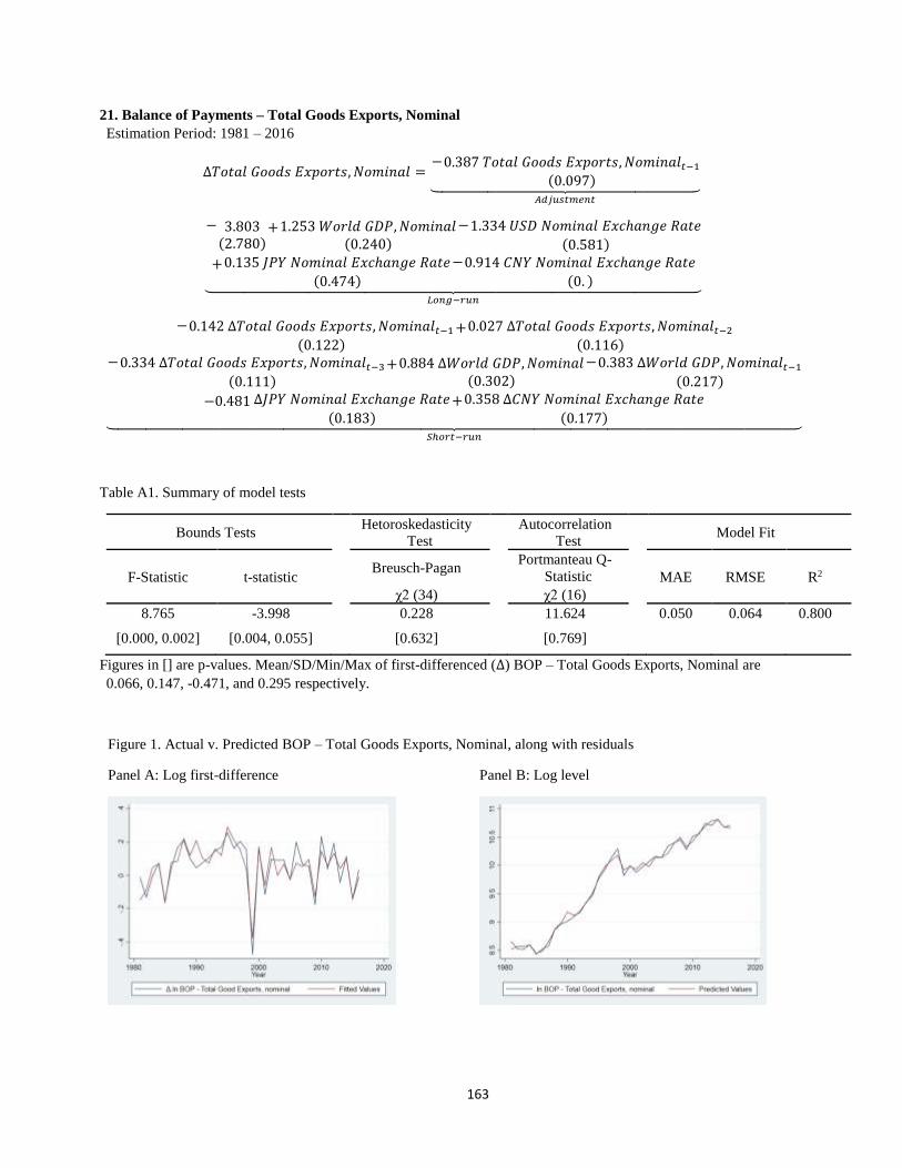
163
21. Balance of Payments – Total Goods Exports, Nominal
Estimation Period: 1981 – 2016
∆𝑇𝑜𝑡𝑎𝑙 𝐺𝑜𝑜𝑑𝑠 𝐸𝑥𝑝𝑜𝑟𝑡𝑠, 𝑁𝑜𝑚𝑖𝑛𝑎𝑙 =−0.387 𝑇𝑜𝑡𝑎𝑙 𝐺𝑜𝑜𝑑𝑠 𝐸𝑥𝑝𝑜𝑟𝑡𝑠, 𝑁𝑜𝑚𝑖𝑛𝑎𝑙𝑡−1
(0.097)⏟ 𝐴𝑑𝑗𝑢𝑠𝑡𝑚𝑒𝑛𝑡
− 3.803(2.780)
+1.253 𝑊𝑜𝑟𝑙𝑑 𝐺𝐷𝑃,𝑁𝑜𝑚𝑖𝑛𝑎𝑙(0.240)
−1.334 𝑈𝑆𝐷 𝑁𝑜𝑚𝑖𝑛𝑎𝑙 𝐸𝑥𝑐ℎ𝑎𝑛𝑔𝑒 𝑅𝑎𝑡𝑒
(0.581)
+0.135 𝐽𝑃𝑌 𝑁𝑜𝑚𝑖𝑛𝑎𝑙 𝐸𝑥𝑐ℎ𝑎𝑛𝑔𝑒 𝑅𝑎𝑡𝑒
(0.474)
−0.914 𝐶𝑁𝑌 𝑁𝑜𝑚𝑖𝑛𝑎𝑙 𝐸𝑥𝑐ℎ𝑎𝑛𝑔𝑒 𝑅𝑎𝑡𝑒
(0. )⏟ 𝐿𝑜𝑛𝑔−𝑟𝑢𝑛
−0.142 ∆𝑇𝑜𝑡𝑎𝑙 𝐺𝑜𝑜𝑑𝑠 𝐸𝑥𝑝𝑜𝑟𝑡𝑠, 𝑁𝑜𝑚𝑖𝑛𝑎𝑙𝑡−1(0.122)
+0.027 ∆𝑇𝑜𝑡𝑎𝑙 𝐺𝑜𝑜𝑑𝑠 𝐸𝑥𝑝𝑜𝑟𝑡𝑠, 𝑁𝑜𝑚𝑖𝑛𝑎𝑙𝑡−2(0.116)
−0.334 ∆𝑇𝑜𝑡𝑎𝑙 𝐺𝑜𝑜𝑑𝑠 𝐸𝑥𝑝𝑜𝑟𝑡𝑠, 𝑁𝑜𝑚𝑖𝑛𝑎𝑙𝑡−3(0.111)
+0.884 ∆𝑊𝑜𝑟𝑙𝑑 𝐺𝐷𝑃,𝑁𝑜𝑚𝑖𝑛𝑎𝑙(0.302)
−0.383 ∆𝑊𝑜𝑟𝑙𝑑 𝐺𝐷𝑃,𝑁𝑜𝑚𝑖𝑛𝑎𝑙𝑡−1(0.217)
−0.481 ∆𝐽𝑃𝑌 𝑁𝑜𝑚𝑖𝑛𝑎𝑙 𝐸𝑥𝑐ℎ𝑎𝑛𝑔𝑒 𝑅𝑎𝑡𝑒
(0.183)+0.358 ∆𝐶𝑁𝑌 𝑁𝑜𝑚𝑖𝑛𝑎𝑙 𝐸𝑥𝑐ℎ𝑎𝑛𝑔𝑒 𝑅𝑎𝑡𝑒
(0.177)⏟ 𝑆ℎ𝑜𝑟𝑡−𝑟𝑢𝑛
Table A1. Summary of model tests
Bounds Tests Hetoroskedasticity
Test Autocorrelation
Test Model Fit
F-Statistic t-statistic Breusch-Pagan Portmanteau Q-
Statistic MAE RMSE R2
χ2 (34) χ2 (16)
8.765 -3.998 0.228 11.624 0.050 0.064 0.800
[0.000, 0.002] [0.004, 0.055] [0.632] [0.769]
Figures in [] are p-values. Mean/SD/Min/Max of first-differenced (∆) BOP – Total Goods Exports, Nominal are
0.066, 0.147, -0.471, and 0.295 respectively.
Figure 1. Actual v. Predicted BOP – Total Goods Exports, Nominal, along with residuals
Panel A: Log first-difference Panel B: Log level
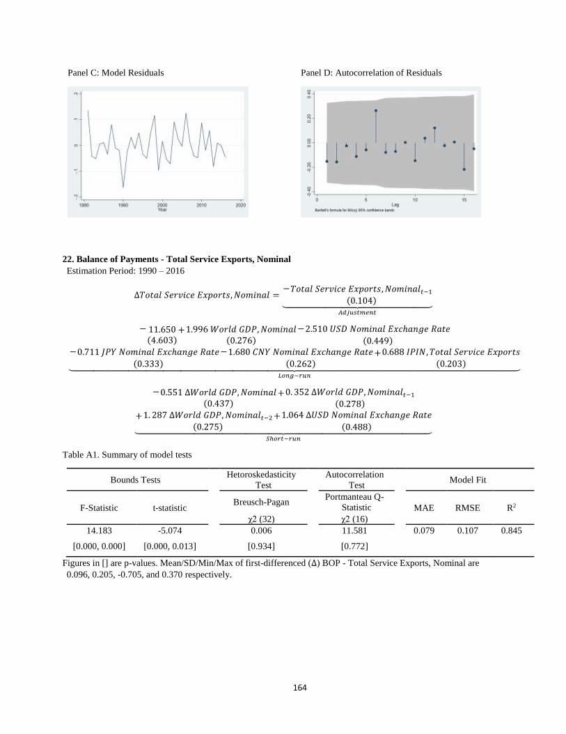
164
Panel C: Model Residuals Panel D: Autocorrelation of Residuals
22. Balance of Payments - Total Service Exports, Nominal
Estimation Period: 1990 – 2016
∆𝑇𝑜𝑡𝑎𝑙 𝑆𝑒𝑟𝑣𝑖𝑐𝑒 𝐸𝑥𝑝𝑜𝑟𝑡𝑠, 𝑁𝑜𝑚𝑖𝑛𝑎𝑙 =−𝑇𝑜𝑡𝑎𝑙 𝑆𝑒𝑟𝑣𝑖𝑐𝑒 𝐸𝑥𝑝𝑜𝑟𝑡𝑠,𝑁𝑜𝑚𝑖𝑛𝑎𝑙𝑡−1
(0.104)⏟ 𝐴𝑑𝑗𝑢𝑠𝑡𝑚𝑒𝑛𝑡
− 11.650(4.603)
+1.996 𝑊𝑜𝑟𝑙𝑑 𝐺𝐷𝑃,𝑁𝑜𝑚𝑖𝑛𝑎𝑙(0.276)
−2.510 𝑈𝑆𝐷 𝑁𝑜𝑚𝑖𝑛𝑎𝑙 𝐸𝑥𝑐ℎ𝑎𝑛𝑔𝑒 𝑅𝑎𝑡𝑒
(0.449)−0.711 𝐽𝑃𝑌 𝑁𝑜𝑚𝑖𝑛𝑎𝑙 𝐸𝑥𝑐ℎ𝑎𝑛𝑔𝑒 𝑅𝑎𝑡𝑒
(0.333)
−1.680 𝐶𝑁𝑌 𝑁𝑜𝑚𝑖𝑛𝑎𝑙 𝐸𝑥𝑐ℎ𝑎𝑛𝑔𝑒 𝑅𝑎𝑡𝑒
(0.262)+0.688 𝐼𝑃𝐼𝑁, 𝑇𝑜𝑡𝑎𝑙 𝑆𝑒𝑟𝑣𝑖𝑐𝑒 𝐸𝑥𝑝𝑜𝑟𝑡𝑠
(0.203)⏟ 𝐿𝑜𝑛𝑔−𝑟𝑢𝑛
−0.551 ∆𝑊𝑜𝑟𝑙𝑑 𝐺𝐷𝑃,𝑁𝑜𝑚𝑖𝑛𝑎𝑙(0.437)
+0. 352 ∆𝑊𝑜𝑟𝑙𝑑 𝐺𝐷𝑃,𝑁𝑜𝑚𝑖𝑛𝑎𝑙𝑡−1(0.278)
+1. 287 ∆𝑊𝑜𝑟𝑙𝑑 𝐺𝐷𝑃,𝑁𝑜𝑚𝑖𝑛𝑎𝑙𝑡−2(0.275)
+1.064 ∆𝑈𝑆𝐷 𝑁𝑜𝑚𝑖𝑛𝑎𝑙 𝐸𝑥𝑐ℎ𝑎𝑛𝑔𝑒 𝑅𝑎𝑡𝑒
(0.488)⏟ 𝑆ℎ𝑜𝑟𝑡−𝑟𝑢𝑛
Table A1. Summary of model tests
Bounds Tests Hetoroskedasticity
Test Autocorrelation
Test Model Fit
F-Statistic t-statistic Breusch-Pagan Portmanteau Q-
Statistic MAE RMSE R2
χ2 (32) χ2 (16)
14.183 -5.074 0.006 11.581 0.079 0.107 0.845
[0.000, 0.000] [0.000, 0.013] [0.934] [0.772]
Figures in [] are p-values. Mean/SD/Min/Max of first-differenced (∆) BOP - Total Service Exports, Nominal are
0.096, 0.205, -0.705, and 0.370 respectively.
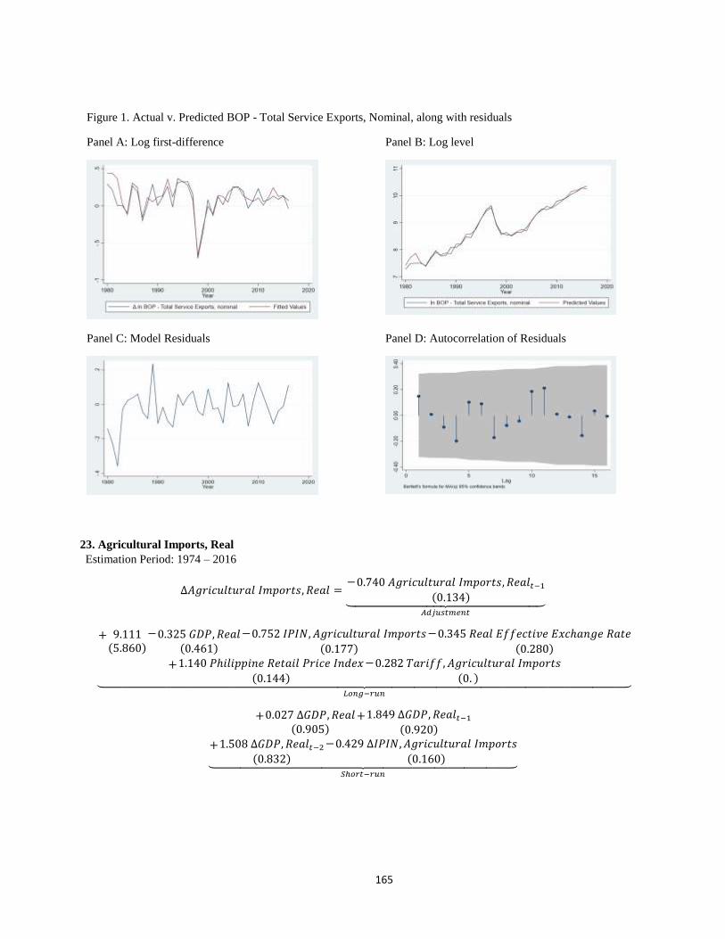
165
Figure 1. Actual v. Predicted BOP - Total Service Exports, Nominal, along with residuals
Panel A: Log first-difference Panel B: Log level
Panel C: Model Residuals Panel D: Autocorrelation of Residuals
23. Agricultural Imports, Real
Estimation Period: 1974 – 2016
∆𝐴𝑔𝑟𝑖𝑐𝑢𝑙𝑡𝑢𝑟𝑎𝑙 𝐼𝑚𝑝𝑜𝑟𝑡𝑠, 𝑅𝑒𝑎𝑙 =−0.740 𝐴𝑔𝑟𝑖𝑐𝑢𝑙𝑡𝑢𝑟𝑎𝑙 𝐼𝑚𝑝𝑜𝑟𝑡𝑠, 𝑅𝑒𝑎𝑙𝑡−1
(0.134)⏟ 𝐴𝑑𝑗𝑢𝑠𝑡𝑚𝑒𝑛𝑡
+ 9.111(5.860)
−0.325 𝐺𝐷𝑃, 𝑅𝑒𝑎𝑙(0.461)
−0.752 𝐼𝑃𝐼𝑁, 𝐴𝑔𝑟𝑖𝑐𝑢𝑙𝑡𝑢𝑟𝑎𝑙 𝐼𝑚𝑝𝑜𝑟𝑡𝑠
(0.177)
−0.345 𝑅𝑒𝑎𝑙 𝐸𝑓𝑓𝑒𝑐𝑡𝑖𝑣𝑒 𝐸𝑥𝑐ℎ𝑎𝑛𝑔𝑒 𝑅𝑎𝑡𝑒
(0.280)
+1.140 𝑃ℎ𝑖𝑙𝑖𝑝𝑝𝑖𝑛𝑒 𝑅𝑒𝑡𝑎𝑖𝑙 𝑃𝑟𝑖𝑐𝑒 𝐼𝑛𝑑𝑒𝑥
(0.144)
−0.282 𝑇𝑎𝑟𝑖𝑓𝑓, 𝐴𝑔𝑟𝑖𝑐𝑢𝑙𝑡𝑢𝑟𝑎𝑙 𝐼𝑚𝑝𝑜𝑟𝑡𝑠
(0. )⏟ 𝐿𝑜𝑛𝑔−𝑟𝑢𝑛
+0.027 ∆𝐺𝐷𝑃, 𝑅𝑒𝑎𝑙(0.905)
+1.849 ∆𝐺𝐷𝑃, 𝑅𝑒𝑎𝑙𝑡−1(0.920)
+1.508 ∆𝐺𝐷𝑃, 𝑅𝑒𝑎𝑙𝑡−2(0.832)
−0.429 ∆𝐼𝑃𝐼𝑁, 𝐴𝑔𝑟𝑖𝑐𝑢𝑙𝑡𝑢𝑟𝑎𝑙 𝐼𝑚𝑝𝑜𝑟𝑡𝑠
(0.160)⏟ 𝑆ℎ𝑜𝑟𝑡−𝑟𝑢𝑛
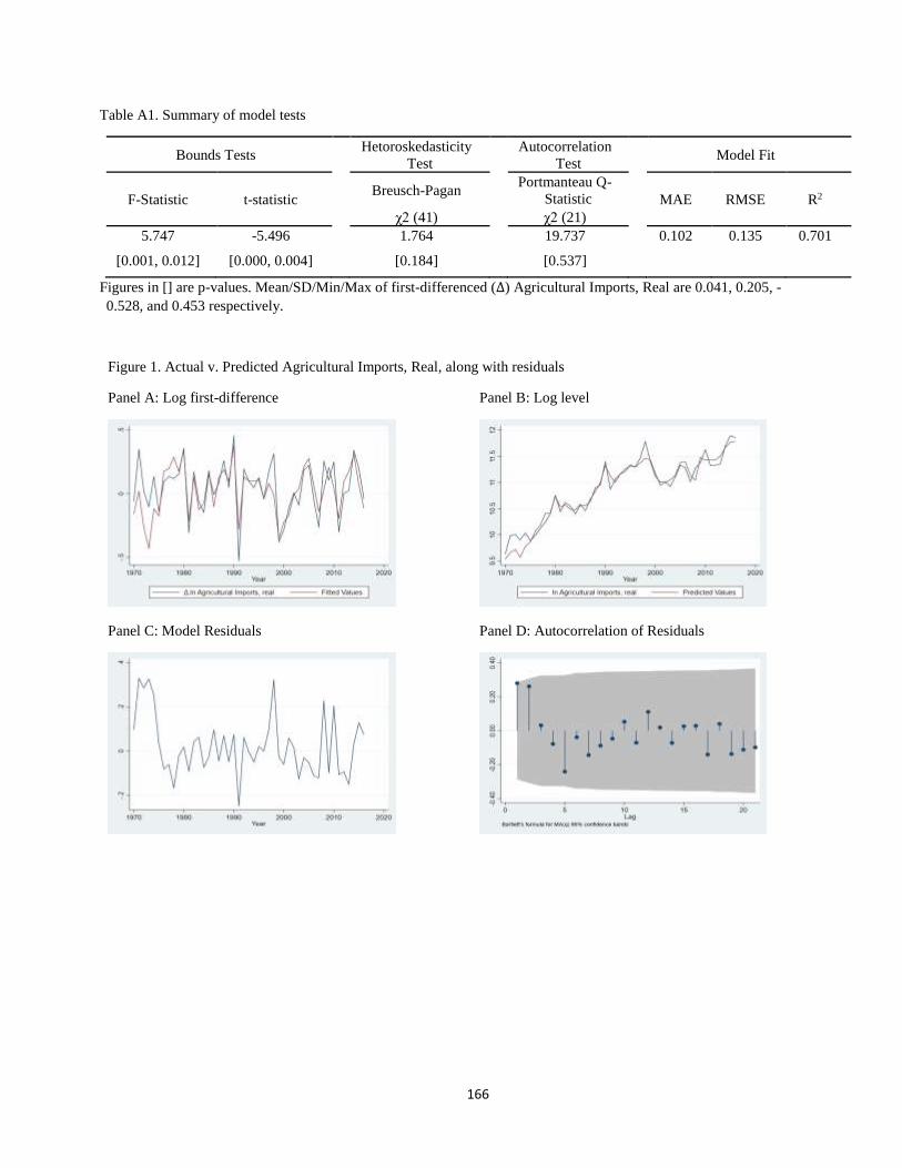
166
Table A1. Summary of model tests
Bounds Tests Hetoroskedasticity
Test Autocorrelation
Test Model Fit
F-Statistic t-statistic Breusch-Pagan Portmanteau Q-
Statistic MAE RMSE R2
χ2 (41) χ2 (21)
5.747 -5.496 1.764 19.737 0.102 0.135 0.701
[0.001, 0.012] [0.000, 0.004] [0.184] [0.537]
Figures in [] are p-values. Mean/SD/Min/Max of first-differenced (∆) Agricultural Imports, Real are 0.041, 0.205, -
0.528, and 0.453 respectively.
Figure 1. Actual v. Predicted Agricultural Imports, Real, along with residuals
Panel A: Log first-difference Panel B: Log level
Panel C: Model Residuals Panel D: Autocorrelation of Residuals

167
24. Fuel Imports, Real
Estimation Period: 1974 – 2016
∆𝐹𝑢𝑒𝑙 𝐼𝑚𝑝𝑜𝑟𝑡𝑠, 𝑅𝑒𝑎𝑙 =−0.484 𝐹𝑢𝑒𝑙 𝐼𝑚𝑝𝑜𝑟𝑡𝑠, 𝑅𝑒𝑎𝑙 𝑡−1
(0.063)⏟ 𝐴𝑑𝑗𝑢𝑠𝑡𝑚𝑒𝑛𝑡
− 2.791(1.390)
+1.261 𝐺𝐷𝑃, 𝑅𝑒𝑎𝑙(0.197)
−0.471 𝐼𝑃𝐼𝑁, 𝐹𝑢𝑒𝑙 𝐼𝑚𝑝𝑜𝑟𝑡𝑠
(0.060)−0.515 𝐶𝑁𝑌 𝑅𝑒𝑎𝑙 𝐸𝑥𝑐ℎ𝑎𝑛𝑔𝑒 𝑅𝑎𝑡𝑒
(0.131)+0.468 𝐽𝑃𝑌 𝑅𝑒𝑎𝑙 𝐸𝑥𝑐ℎ𝑎𝑛𝑔𝑒 𝑅𝑎𝑡𝑒
(0.171)⏟ 𝐿𝑜𝑛𝑔−𝑟𝑢𝑛
+0.286 ∆𝐶𝑁𝑌 𝑅𝑒𝑎𝑙 𝐸𝑥𝑐ℎ𝑎𝑛𝑔𝑒 𝑅𝑎𝑡𝑒
(0.119)
−0.366 ∆𝐽𝑃𝑌 𝑅𝑒𝑎𝑙 𝐸𝑥𝑐ℎ𝑎𝑛𝑔𝑒 𝑅𝑎𝑡𝑒
(0.103)−0.083 ∆𝐽𝑃𝑌 𝑅𝑒𝑎𝑙 𝐸𝑥𝑐ℎ𝑎𝑛𝑔𝑒 𝑅𝑎𝑡𝑒𝑡−1
(0.098)
−0.243 ∆𝐽𝑃𝑌 𝑅𝑒𝑎𝑙 𝐸𝑥𝑐ℎ𝑎𝑛𝑔𝑒 𝑅𝑎𝑡𝑒𝑡−2(0.091)⏟
𝑆ℎ𝑜𝑟𝑡−𝑟𝑢𝑛
Table A1. Summary of model tests
Bounds Tests Hetoroskedasticity
Test Autocorrelation
Test Model Fit
F-Statistic t-statistic Breusch-Pagan Portmanteau Q-
Statistic MAE RMSE R2
χ2 (41) χ2 (20)
15.015 -7.688 0.755 26.433 0.043 0.059 0.709
[0.000, 0.000] [0.000, 0.000] [0.384] [0.151]
Figures in [] are p-values. Mean/SD/Min/Max of first-differenced (∆) Fuel Imports, Real are 0.020, 0.104, -0.304,
and 0.264 respectively.
Figure 1. Actual v. Predicted Fuel Imports, Real, along with residuals
Panel A: Log first-difference Panel B: Log level

168
Panel C: Model Residuals Panel D: Autocorrelation of Residuals
25. Machinery Imports, Real
Estimation Period: 1974 – 2016
∆𝑀𝑎𝑐ℎ𝑖𝑛𝑒𝑟𝑦 𝐼𝑚𝑝𝑜𝑟𝑡𝑠, 𝑅𝑒𝑎𝑙 =−0.360 𝑀𝑎𝑐ℎ𝑖𝑛𝑒𝑟𝑦 𝐼𝑚𝑝𝑜𝑟𝑡𝑠, 𝑅𝑒𝑎𝑙𝑡−1
(0.060)⏟ 𝐴𝑑𝑗𝑢𝑠𝑡𝑚𝑒𝑛𝑡
− 7.806(3.850)
+2.548 𝐺𝐷𝑃, 𝑅𝑒𝑎𝑙(0.712)
+0.572 𝐼𝑃𝐼𝑁,𝑀𝑎𝑐ℎ𝑖𝑛𝑒𝑟𝑦 𝐼𝑚𝑝𝑜𝑟𝑡𝑠
(0.179)
−0.971 𝐹𝑜𝑟𝑒𝑖𝑔𝑛 𝐼𝑃𝐼𝑁,𝑀𝑎𝑐ℎ𝑖𝑛𝑒𝑟𝑦 𝐼𝑚𝑝𝑜𝑟𝑡𝑠
(0.170)−1.124 𝑅𝑒𝑎𝑙 𝐸𝑓𝑓𝑒𝑐𝑡𝑖𝑣𝑒 𝐸𝑥𝑐ℎ𝑎𝑛𝑔𝑒 𝑅𝑎𝑡𝑒
(0.389)+1.078 𝑇𝑎𝑟𝑖𝑓𝑓,𝑀𝑎𝑐ℎ𝑖𝑛𝑒𝑟𝑦 𝐼𝑚𝑝𝑜𝑟𝑡𝑠
(0.339)⏟ 𝐿𝑜𝑛𝑔−𝑟𝑢𝑛
+0.305 ∆𝑀𝑎𝑐ℎ𝑖𝑛𝑒𝑟𝑦 𝐼𝑚𝑝𝑜𝑟𝑡𝑠, 𝑅𝑒𝑎𝑙𝑡−1(0.104)
+1.663 ∆𝐺𝐷𝑃, 𝑅𝑒𝑎𝑙(0.805)
+0.190 ∆𝐹𝑜𝑟𝑒𝑖𝑔𝑛 𝐼𝑃𝐼𝑁,𝑀𝑎𝑐ℎ𝑖𝑛𝑒𝑟𝑦 𝐼𝑚𝑝𝑜𝑟𝑡𝑠
(0.074)
−0.435 ∆𝑇𝑎𝑟𝑖𝑓𝑓,𝑀𝑎𝑐ℎ𝑖𝑛𝑒𝑟𝑦 𝐼𝑚𝑝𝑜𝑟𝑡𝑠
(0.173)⏟ 𝑆ℎ𝑜𝑟𝑡−𝑟𝑢𝑛
Table A1. Summary of model tests
Bounds Tests Hetoroskedasticity
Test Autocorrelation
Test Model Fit
F-Statistic t-statistic Breusch-Pagan Portmanteau Q-
Statistic MAE RMSE R2
χ2 (41) χ2 (21)
8.536 -5.920 0.725 10.085 0.094 0.140 0.792
[0.000, 0.001] [0.000, 0.002] [0.394] [0.977]
Figures in [] are p-values. Mean/SD/Min/Max of first-differenced (∆) Machinery Imports, Real are 0.053, 0.207, -
0.512, and 0.441 respectively.

169
Figure 1. Actual v. Predicted Machinery Imports, Real, along with residuals
Panel A: Log first-difference Panel B: Log level
Panel C: Model Residuals Panel D: Autocorrelation of Residuals
26. Materials Imports, Real
Estimation Period: 1974 – 2017
∆𝑀𝑎𝑡𝑒𝑟𝑖𝑎𝑙𝑠 𝐼𝑚𝑝𝑜𝑟𝑡𝑠, 𝑅𝑒𝑎𝑙 =−0.693 𝑀𝑎𝑡𝑒𝑟𝑖𝑎𝑙𝑠 𝐼𝑚𝑝𝑜𝑟𝑡𝑠, 𝑅𝑒𝑎𝑙 𝑡−1
(0.109)⏟ 𝐴𝑑𝑗𝑢𝑠𝑡𝑚𝑒𝑛𝑡
− 5.254(2.032)
+1.592 𝐺𝐷𝑃, 𝑅𝑒𝑎𝑙(0.212)
−0.653 𝐹𝑜𝑟𝑒𝑖𝑔𝑛 𝐼𝑃𝐼𝑁,𝑀𝑎𝑡𝑒𝑟𝑖𝑎𝑙𝑠 𝐼𝑚𝑝𝑜𝑟𝑡𝑠
(0.216)−0.853 𝑇𝑎𝑟𝑖𝑓𝑓,𝑀𝑎𝑡𝑒𝑟𝑖𝑎𝑙𝑠 𝐼𝑚𝑝𝑜𝑟𝑡𝑠
(0.160)+0.130 𝐼𝑃𝐼𝑁,𝑀𝑎𝑐ℎ𝑖𝑛𝑒𝑟𝑦 𝐼𝑚𝑝𝑜𝑟𝑡𝑠
(0.127)⏟ 𝐿𝑜𝑛𝑔−𝑟𝑢𝑛
+0.332 ∆𝑀𝑎𝑡𝑒𝑟𝑖𝑎𝑙𝑠 𝐼𝑚𝑝𝑜𝑟𝑡𝑠𝑡−1(0.131)
+0. 333 ∆𝑀𝑎𝑡𝑒𝑟𝑖𝑎𝑙𝑠 𝐼𝑚𝑝𝑜𝑟𝑡𝑠𝑡−2(0.114)
+1.849 ∆𝐺𝐷𝑃, 𝑅𝑒𝑎𝑙(0.806)
−1. 945 ∆𝐺𝐷𝑃, 𝑅𝑒𝑎𝑙𝑡−1(0.973)
−1.451 ∆𝐺𝐷𝑃, 𝑅𝑒𝑎𝑡−2𝑙
(0.154)+3. 612 ∆𝐺𝐷𝑃, 𝑅𝑒𝑎𝑙𝑡−3
(0.985)
+0.597 ∆𝐹𝑜𝑟𝑒𝑖𝑔𝑛 𝐼𝑃𝐼𝑁,𝑀𝑎𝑡𝑒𝑟𝑖𝑎𝑙 𝐼𝑚𝑝𝑜𝑟𝑡𝑠
(0.227)+0.830 ∆𝐹𝑜𝑟𝑒𝑖𝑔𝑛 𝐼𝑃𝐼𝑁,𝑀𝑎𝑡𝑒𝑟𝑖𝑎𝑙 𝐼𝑚𝑝𝑜𝑟𝑡𝑠𝑡−1
(0.239)−0.833 ∆𝐼𝑃𝐼𝑁,𝑀𝑎𝑐ℎ𝑖𝑛𝑒𝑟𝑦 𝐼𝑚𝑝𝑜𝑟𝑡𝑠
(0.150)
−0.352 ∆𝐼𝑃𝐼𝑁,𝑀𝑎𝑐ℎ𝑖𝑛𝑒𝑟𝑦 𝐼𝑚𝑝𝑜𝑟𝑡𝑠𝑡−1(0.201)⏟
𝑆ℎ𝑜𝑟𝑡−𝑟𝑢𝑛
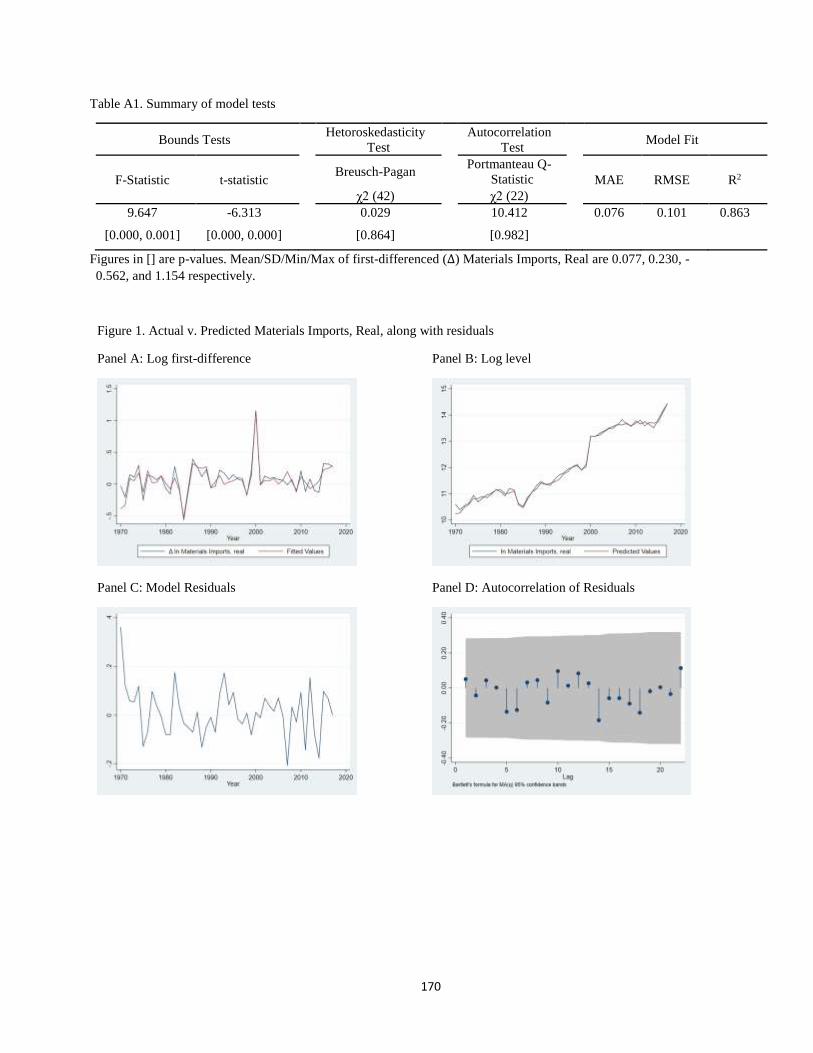
170
Table A1. Summary of model tests
Bounds Tests Hetoroskedasticity
Test Autocorrelation
Test Model Fit
F-Statistic t-statistic Breusch-Pagan Portmanteau Q-
Statistic MAE RMSE R2
χ2 (42) χ2 (22)
9.647 -6.313 0.029 10.412 0.076 0.101 0.863
[0.000, 0.001] [0.000, 0.000] [0.864] [0.982]
Figures in [] are p-values. Mean/SD/Min/Max of first-differenced (∆) Materials Imports, Real are 0.077, 0.230, -
0.562, and 1.154 respectively.
Figure 1. Actual v. Predicted Materials Imports, Real, along with residuals
Panel A: Log first-difference Panel B: Log level
Panel C: Model Residuals Panel D: Autocorrelation of Residuals

171
27. Other Goods Imports, Real
Estimation Period: 1971 – 2016
∆𝑂𝑡ℎ𝑒𝑟 𝐺𝑜𝑜𝑑𝑠 𝐼𝑚𝑝𝑜𝑟𝑡𝑠, 𝑅𝑒𝑎𝑙 =−0.319 𝑂𝑡ℎ𝑒𝑟 𝐺𝑜𝑜𝑑𝑠 𝐼𝑚𝑝𝑜𝑟𝑡𝑠, 𝑅𝑒𝑎𝑙𝑡−1
(0.085)⏟ 𝐴𝑑𝑗𝑢𝑠𝑡𝑚𝑒𝑛𝑡
+ 11.368(3.155)
−1.567 𝐺𝐷𝑃, 𝑅𝑒𝑎𝑙(0.824)
+0.323 𝐼𝑃𝐼𝑁, 𝑂𝑡ℎ𝑒𝑟 𝐺𝑜𝑜𝑑𝑠 𝐼𝑚𝑝𝑜𝑟𝑡𝑠
(0.246)
+0.839 𝑃ℎ𝑖𝑙𝑖𝑝𝑝𝑖𝑛𝑒 𝑊ℎ𝑜𝑙𝑒𝑠𝑎𝑙𝑒 𝑃𝑟𝑖𝑐𝑒 𝐼𝑛𝑑𝑒𝑥(0.238)
−0.870 𝑅𝑒𝑎𝑙 𝐸𝑓𝑓𝑒𝑐𝑡𝑖𝑣𝑒 𝐸𝑥𝑐ℎ𝑎𝑛𝑔𝑒 𝑅𝑎𝑡𝑒
(0.558)⏟ 𝐿𝑜𝑛𝑔−𝑟𝑢𝑛
+1.933 ∆𝐺𝐷𝑃, 𝑅𝑒𝑎𝑙(0.966)
−0.748 ∆𝐼𝑃𝐼𝑁, 𝑂𝑡ℎ𝑒𝑟 𝐺𝑜𝑜𝑑𝑠 𝐼𝑚𝑝𝑜𝑟𝑡𝑠(0.135)
−0.106 ∆𝐼𝑃𝐼𝑁, 𝑂𝑡ℎ𝑒𝑟 𝐺𝑜𝑜𝑑𝑠 𝐼𝑚𝑝𝑜𝑟𝑡𝑠𝑡−1(0.134)
+0.411 ∆𝐼𝑃𝐼𝑁, 𝑂𝑡ℎ𝑒𝑟 𝐺𝑜𝑜𝑑𝑠 𝐼𝑚𝑝𝑜𝑟𝑡𝑠𝑡−2(0.129)
−0.363 ∆𝐼𝑃𝐼𝑁, 𝑂𝑡ℎ𝑒𝑟 𝐺𝑜𝑜𝑑𝑠 𝐼𝑚𝑝𝑜𝑟𝑡𝑠𝑡−3(0.113)
+0.481∆𝑃ℎ𝑖𝑙𝑖𝑝𝑝𝑖𝑛𝑒 𝑊ℎ𝑜𝑙𝑒𝑠𝑎𝑙𝑒 𝑃𝑟𝑖𝑐𝑒 𝐼𝑛𝑑𝑒𝑥(0.242)
−0631 ∆𝑃ℎ𝑖𝑙𝑖𝑝𝑝𝑖𝑛𝑒 𝑊ℎ𝑜𝑙𝑒𝑠𝑎𝑙𝑒 𝑃𝑟𝑖𝑐𝑒 𝐼𝑛𝑑𝑒𝑥𝑡−1(0.245)
+0.249 ∆𝑅𝑒𝑎𝑙 𝐸𝑓𝑓𝑒𝑐𝑡𝑖𝑣𝑒 𝐸𝑥𝑐ℎ𝑎𝑛𝑔𝑒 𝑅𝑎𝑡𝑒
(0.199)+0.274 ∆𝑅𝑒𝑎𝑙 𝐸𝑓𝑓𝑒𝑐𝑡𝑖𝑣𝑒 𝐸𝑥𝑐ℎ𝑎𝑛𝑔𝑒 𝑅𝑎𝑡𝑒𝑡−1
(0.167)
+0.703 ∆𝑅𝑒𝑎𝑙 𝐸𝑓𝑓𝑒𝑐𝑡𝑖𝑣𝑒 𝐸𝑥𝑐ℎ𝑎𝑛𝑔𝑒 𝑅𝑎𝑡𝑒𝑡−2(0.154)
+0.368 ∆𝑅𝑒𝑎𝑙 𝐸𝑓𝑓𝑒𝑐𝑡𝑖𝑣𝑒 𝐸𝑥𝑐ℎ𝑎𝑛𝑔𝑒 𝑅𝑎𝑡𝑒𝑡−3(0.153)⏟
𝑆ℎ𝑜𝑟𝑡−𝑟𝑢𝑛
Table A1. Summary of model tests
Bounds Tests Hetoroskedasticity
Test Autocorrelation
Test Model Fit
F-Statistic t-statistic Breusch-Pagan Portmanteau Q-
Statistic MAE RMSE R2
χ2 (44) χ2 (21)
7.346 -3.719 1.377 25.455 0.055 0.067 0.838
[0.000, 0.004] [0.007, 0.079] [0.240] [0.227]
Figures in [] are p-values. Mean/SD/Min/Max of first-differenced (∆) Other Goods Imports, Real are 0.064, 0.192, -
0.618, and 0.404 respectively.
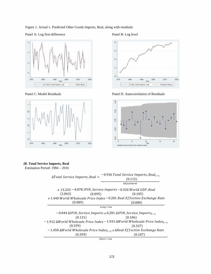
172
Figure 1. Actual v. Predicted Other Goods Imports, Real, along with residuals
Panel A: Log first-difference Panel B: Log level
Panel C: Model Residuals Panel D: Autocorrelation of Residuals
28. Total Service Imports, Real
Estimation Period: 1984 – 2016
∆𝑇𝑜𝑡𝑎𝑙 𝑆𝑒𝑟𝑣𝑖𝑐𝑒 𝐼𝑚𝑝𝑜𝑟𝑡𝑠, 𝑅𝑒𝑎𝑙 =−0.936 𝑇𝑜𝑡𝑎𝑙 𝑆𝑒𝑟𝑣𝑖𝑐𝑒 𝐼𝑚𝑝𝑜𝑟𝑡𝑠, 𝑅𝑒𝑎𝑙𝑡−1
(0.115)⏟ 𝐴𝑑𝑗𝑢𝑠𝑡𝑚𝑒𝑛𝑡
+ 13.243(2.063)
−0.878 𝐼𝑃𝐼𝑁, 𝑆𝑒𝑟𝑣𝑖𝑐𝑒 𝐼𝑚𝑝𝑜𝑟𝑡𝑠
(0.095)
−0.334 𝑊𝑜𝑟𝑙𝑑 𝐺𝐷𝑃, 𝑅𝑒𝑎𝑙(0.105)
+1.440 𝑊𝑜𝑟𝑙𝑑 𝑊ℎ𝑜𝑙𝑒𝑠𝑎𝑙𝑒 𝑃𝑟𝑖𝑐𝑒 𝐼𝑛𝑑𝑒𝑥(0.089)
−0.281 𝑅𝑒𝑎𝑙 𝐸𝑓𝑓𝑒𝑐𝑡𝑖𝑣𝑒 𝐸𝑥𝑐ℎ𝑎𝑛𝑔𝑒 𝑅𝑎𝑡𝑒
(0.080)⏟ 𝐿𝑜𝑛𝑔−𝑟𝑢𝑛
−0.044 ∆𝐼𝑃𝐼𝑁, 𝑆𝑒𝑟𝑣𝑖𝑐𝑒 𝐼𝑚𝑝𝑜𝑟𝑡𝑠
(0.131)+0.281 ∆𝐼𝑃𝐼𝑁, 𝑆𝑒𝑟𝑣𝑖𝑐𝑒 𝐼𝑚𝑝𝑜𝑟𝑡𝑠𝑡−1
(0.106)−1.912 ∆𝑊𝑜𝑟𝑙𝑑 𝑊ℎ𝑜𝑙𝑒𝑠𝑎𝑙𝑒 𝑃𝑟𝑖𝑐𝑒 𝐼𝑛𝑑𝑒𝑥
(0.339)−1.933 ∆𝑊𝑜𝑟𝑙𝑑 𝑊ℎ𝑜𝑙𝑒𝑠𝑎𝑙𝑒 𝑃𝑟𝑖𝑐𝑒 𝐼𝑛𝑑𝑒𝑥𝑡−1
(0.337)−1.458 ∆𝑊𝑜𝑟𝑙𝑑 𝑊ℎ𝑜𝑙𝑒𝑠𝑎𝑙𝑒 𝑃𝑟𝑖𝑐𝑒 𝐼𝑛𝑑𝑒𝑥𝑡−2
(0.359)+∆𝑅𝑒𝑎𝑙 𝐸𝑓𝑓𝑒𝑐𝑡𝑖𝑣𝑒 𝐸𝑥𝑐ℎ𝑎𝑛𝑔𝑒 𝑅𝑎𝑡𝑒
(0.107)⏟ 𝑆ℎ𝑜𝑟𝑡−𝑟𝑢𝑛

173
Table A1. Summary of model tests
Bounds Tests Hetoroskedasticity
Test Autocorrelation
Test Model Fit
F-Statistic t-statistic Breusch-Pagan Portmanteau Q-
Statistic MAE RMSE R2
χ2 (31) χ2 (15)
17.133 -8.091 1.982 7.753 0.057 0.105 0.878
[0.000, 0.000] [0.000, 0.000] [0.159] [0.933]
Figures in [] are p-values. Mean/SD/Min/Max of first-differenced (∆) Total Service Imports, Real are 0.067, 0.123, -
0.148, and 0.483 respectively.
Figure 1. Actual v. Predicted Total Service Imports, Real, along with residuals
Panel A: Log first-difference Panel B: Log level
Panel C: Model Residuals Panel D: Autocorrelation of Residuals

174
29. Balance of Payments – Total Goods Imports, Nominal
Estimation Period: 1981 – 2016
∆𝑇𝑜𝑡𝑎𝑙 𝐺𝑜𝑜𝑑𝑠 𝐼𝑚𝑝𝑜𝑟𝑡𝑠, 𝑁𝑜𝑚𝑖𝑛𝑎𝑙 =−0.564 𝑇𝑜𝑡𝑎𝑙 𝐺𝑜𝑜𝑑𝑠 𝐼𝑚𝑝𝑜𝑟𝑡𝑠, 𝑁𝑜𝑚𝑖𝑛𝑎𝑙𝑡−1
(0.089)⏟ 𝐴𝑑𝑗𝑢𝑠𝑡𝑚𝑒𝑛𝑡
+ 7.300(1.554)
−0.602 𝐺𝐷𝑃,𝑁𝑜𝑚𝑖𝑛𝑎𝑙(0.271)
+1.749 𝑊𝑜𝑟𝑙𝑑 𝑊ℎ𝑜𝑙𝑒𝑠𝑎𝑙𝑒 𝑃𝑟𝑖𝑐𝑒 𝐼𝑛𝑑𝑒𝑥(0.315)
−0.509 𝑈𝑆𝐷 𝑁𝑜𝑚𝑖𝑛𝑎𝑙 𝐸𝑥𝑐ℎ𝑎𝑛𝑔𝑒 𝑅𝑎𝑡𝑒
(0.095)+0.254 𝐶𝑁𝑌 𝑁𝑜𝑚𝑖𝑛𝑎𝑙 𝐸𝑥𝑐ℎ𝑎𝑛𝑔𝑒 𝑅𝑎𝑡𝑒
(0.197)⏟ 𝐿𝑜𝑛𝑔−𝑟𝑢𝑛
+0.030 ∆𝑇𝑜𝑡𝑎𝑙 𝐺𝑜𝑜𝑑𝑠 𝐼𝑚𝑝𝑜𝑟𝑡𝑠, 𝑁𝑜𝑚𝑖𝑛𝑎𝑙𝑡−1(0.108)
+0.189 ∆𝑇𝑜𝑡𝑎𝑙 𝐺𝑜𝑜𝑑𝑠 𝐼𝑚𝑝𝑜𝑟𝑡𝑠, 𝑁𝑜𝑚𝑖𝑛𝑎𝑙𝑡−2(0.081)
+0.841 ∆𝐺𝐷𝑃,𝑁𝑜𝑚𝑖𝑛𝑎𝑙(0.260)
+0.430 ∆𝐺𝐷𝑃,𝑁𝑜𝑚𝑖𝑛𝑎𝑙𝑡−1(0.267)
−0.030 ∆𝑊𝑜𝑟𝑙𝑑 𝑊ℎ𝑜𝑙𝑒𝑠𝑎𝑙𝑒 𝑃𝑟𝑖𝑐𝑒 𝐼𝑛𝑑𝑒𝑥(0.269)
−1.128 ∆𝑊𝑜𝑟𝑙𝑑 𝑊ℎ𝑜𝑙𝑒𝑠𝑎𝑙𝑒 𝑃𝑟𝑖𝑐𝑒 𝐼𝑛𝑑𝑒𝑥𝑡−1(0.272)
−0.427 ∆𝑈𝑆𝐷 𝑁𝑜𝑚𝑖𝑛𝑎𝑙 𝐸𝑥𝑐ℎ𝑎𝑛𝑔𝑒 𝑅𝑎𝑡𝑒
(0.136)
−0.766 ∆𝑈𝑆𝐷 𝑁𝑜𝑚𝑖𝑛𝑎𝑙 𝐸𝑥𝑐ℎ𝑎𝑛𝑔𝑒 𝑅𝑎𝑡𝑒𝑡−1(0.146)⏟
𝑆ℎ𝑜𝑟𝑡−𝑟𝑢𝑛
Table A1. Summary of model tests
Bounds Tests Hetoroskedasticity
Test Autocorrelation
Test Model Fit
F-Statistic t-statistic Breusch-Pagan Portmanteau Q-
Statistic MAE RMSE R2
χ2 (34) χ2 (16)
12.927 -6.329 0.376 22.388 0.031 0.038 0.915
[0.000, 0.000] [0.000, 0.001] [0.539] [0.131]
Figures in [] are p-values. Mean/SD/Min/Max of first-differenced (∆) BOP – Total Goods Imports, Nominal are
0.076, 0.137, -0.215, and 0.289 respectively.
Figure 1. Actual v. Predicted BOP – Total Goods Imports, Nominal, along with residuals
Panel A: Log first-difference Panel B: Log level

175
Panel C: Model Residuals Panel D: Autocorrelation of Residuals
30. Balance of Payments – Total Service Imports, Nominal
Estimation Period: 1981 – 2016
∆𝑇𝑜𝑡𝑎𝑙 𝑆𝑒𝑟𝑣𝑖𝑐𝑒 𝐼𝑚𝑝𝑜𝑟𝑡𝑠, 𝑁𝑜𝑚𝑖𝑛𝑎𝑙 =−0.954 𝑇𝑜𝑡𝑎𝑙 𝑆𝑒𝑟𝑣𝑖𝑐𝑒 𝐼𝑚𝑝𝑜𝑟𝑡𝑠, 𝑁𝑜𝑚𝑖𝑛𝑎𝑙𝑡−1
(0.101)⏟ 𝐴𝑑𝑗𝑢𝑠𝑡𝑚𝑒𝑛𝑡
+ 18.277(2.062)
−1.406 𝐺𝐷𝑃,𝑁𝑜𝑚𝑖𝑛𝑎𝑙(0.117)
+2.925 𝑊𝑜𝑟𝑙𝑑 𝑊ℎ𝑜𝑙𝑒𝑠𝑎𝑙𝑒 𝑃𝑟𝑖𝑐𝑒 𝐼𝑛𝑑𝑒𝑥(0.148)
−1.092 𝑁𝑜𝑚𝑖𝑛𝑎𝑙 𝐸𝑓𝑓𝑒𝑐𝑡𝑖𝑣𝑒 𝐸𝑥𝑐ℎ𝑎𝑛𝑔𝑒 𝑅𝑎𝑡𝑒
(0.061)⏟ 𝐿𝑜𝑛𝑔−𝑟𝑢𝑛
+0.332 ∆𝑇𝑜𝑡𝑎𝑙 𝑆𝑒𝑟𝑣𝑖𝑐𝑒 𝐼𝑚𝑝𝑜𝑟𝑡𝑠, 𝑁𝑜𝑚𝑖𝑛𝑎𝑙𝑡−1(0.081)
+1.101 ∆𝐺𝐷𝑃,𝑁𝑜𝑚𝑖𝑛𝑎𝑙(0.430)
+0.940 ∆𝐺𝐷𝑃,𝑁𝑜𝑚𝑖𝑛𝑎𝑙𝑡−1(0.440)
−1.609 ∆𝑊𝑜𝑟𝑙𝑑 𝑊ℎ𝑜𝑙𝑒𝑠𝑎𝑙𝑒 𝑃𝑟𝑖𝑐𝑒 𝐼𝑛𝑑𝑒𝑥(0.492)
−2.704 ∆𝑊𝑜𝑟𝑙𝑑 𝑊ℎ𝑜𝑙𝑒𝑠𝑎𝑙𝑒 𝑃𝑟𝑖𝑐𝑒 𝐼𝑛𝑑𝑒𝑥𝑡−1(0.521)
+0.640 ∆𝑁𝑜𝑚𝑖𝑛𝑎𝑙 𝐸𝑓𝑓𝑒𝑐𝑡𝑖𝑣𝑒 𝐸𝑥𝑐ℎ𝑎𝑛𝑔𝑒 𝑅𝑎𝑡𝑒
(0.182)⏟ 𝑆ℎ𝑜𝑟𝑡−𝑟𝑢𝑛
Table A1. Summary of model tests
Bounds Tests Hetoroskedasticity
Test Autocorrelation
Test Model Fit
F-Statistic t-statistic Breusch-Pagan Portmanteau Q-
Statistic MAE RMSE R2
χ2 (34) χ2 (17)
23.367 -9.401 0.093 12.114 0.065 0.082 0.895
[0.000, 0.000] [0.000, 0.000] [0.760] [0.793]
Figures in [] are p-values. Mean/SD/Min/Max of first-differenced (∆) BOP – Total Service Imports, Nominal are
0.085, 0.226, -0.674, and 0.409 respectively.
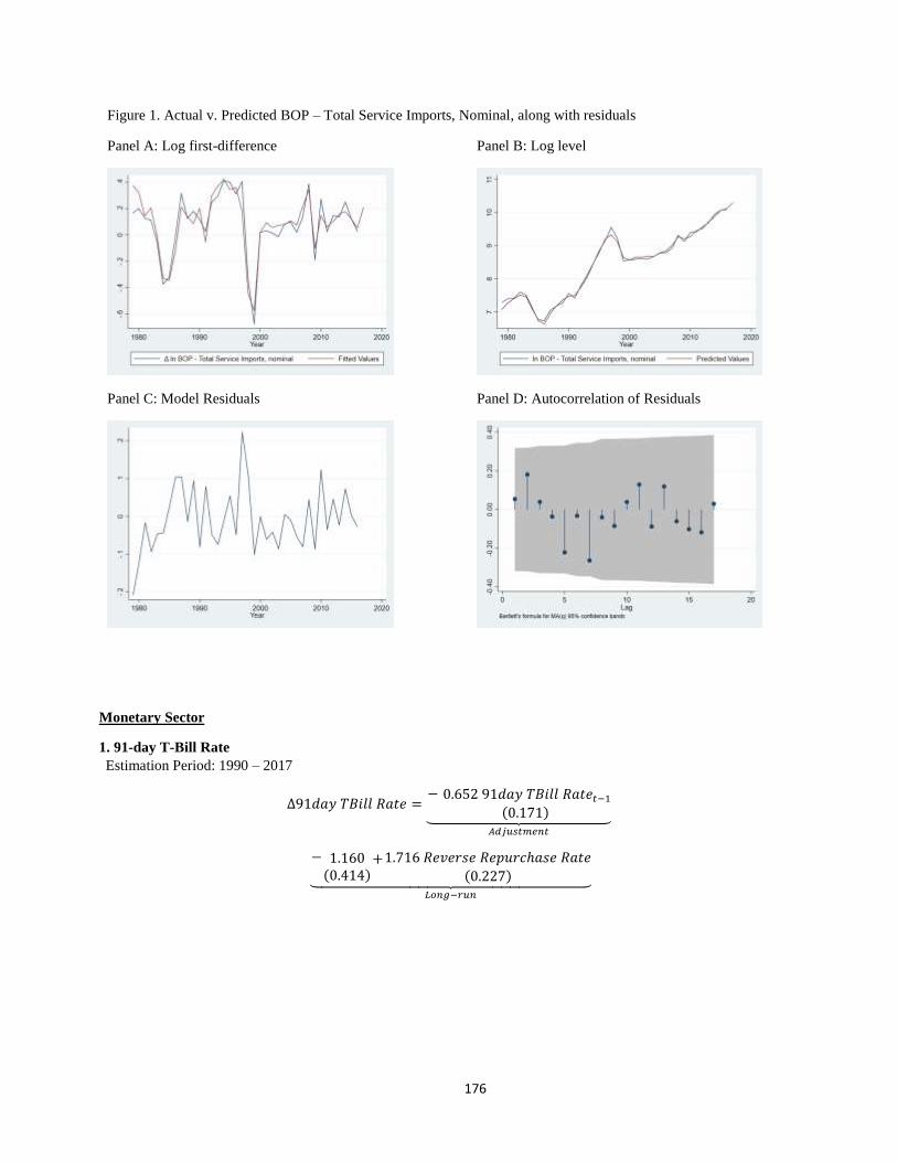
176
Figure 1. Actual v. Predicted BOP – Total Service Imports, Nominal, along with residuals
Panel A: Log first-difference Panel B: Log level
Panel C: Model Residuals Panel D: Autocorrelation of Residuals
Monetary Sector
1. 91-day T-Bill Rate
Estimation Period: 1990 – 2017
∆91𝑑𝑎𝑦 𝑇𝐵𝑖𝑙𝑙 𝑅𝑎𝑡𝑒 =− 0.652 91𝑑𝑎𝑦 𝑇𝐵𝑖𝑙𝑙 𝑅𝑎𝑡𝑒𝑡−1
(0.171)⏟ 𝐴𝑑𝑗𝑢𝑠𝑡𝑚𝑒𝑛𝑡
− 1.160(0.414)
+1.716 𝑅𝑒𝑣𝑒𝑟𝑠𝑒 𝑅𝑒𝑝𝑢𝑟𝑐ℎ𝑎𝑠𝑒 𝑅𝑎𝑡𝑒(0.227)⏟
𝐿𝑜𝑛𝑔−𝑟𝑢𝑛
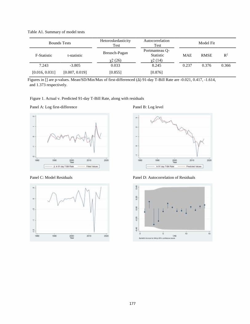
177
Table A1. Summary of model tests
Bounds Tests Hetoroskedasticity
Test Autocorrelation
Test Model Fit
F-Statistic t-statistic Breusch-Pagan Portmanteau Q-
Statistic MAE RMSE R2
χ2 (26) χ2 (14)
7.243 -3.805 0.033 8.245 0.237 0.376 0.366
[0.016, 0.031] [0.007, 0.019] [0.855] [0.876]
Figures in [] are p-values. Mean/SD/Min/Max of first-differenced (∆) 91-day T-Bill Rate are -0.021, 0.417, -1.614,
and 1.373 respectively.
Figure 1. Actual v. Predicted 91-day T-Bill Rate, along with residuals
Panel A: Log first-difference Panel B: Log level
Panel C: Model Residuals Panel D: Autocorrelation of Residuals
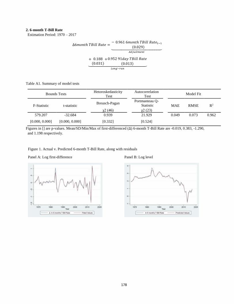
178
2. 6-month T-Bill Rate
Estimation Period: 1970 – 2017
∆6𝑚𝑜𝑛𝑡ℎ 𝑇𝐵𝑖𝑙𝑙 𝑅𝑎𝑡𝑒 =− 0.961 6𝑚𝑜𝑛𝑡ℎ 𝑇𝐵𝑖𝑙𝑙 𝑅𝑎𝑡𝑒𝑡−1
(0.029)⏟ 𝐴𝑑𝑗𝑢𝑠𝑡𝑚𝑒𝑛𝑡
+ 0.188(0.031)
+0.952 91𝑑𝑎𝑦 𝑇𝐵𝑖𝑙𝑙 𝑅𝑎𝑡𝑒(0.013)⏟
𝐿𝑜𝑛𝑔−𝑟𝑢𝑛
Table A1. Summary of model tests
Bounds Tests Hetoroskedasticity
Test Autocorrelation
Test Model Fit
F-Statistic t-statistic Breusch-Pagan Portmanteau Q-
Statistic MAE RMSE R2
χ2 (46) χ2 (23)
579.207 -32.684 0.939 21.929 0.049 0.073 0.962
[0.000, 0.000] [0.000, 0.000] [0.332] [0.524]
Figures in [] are p-values. Mean/SD/Min/Max of first-differenced (∆) 6-month T-Bill Rate are -0.019, 0.383, -1.290,
and 1.198 respectively.
Figure 1. Actual v. Predicted 6-month T-Bill Rate, along with residuals
Panel A: Log first-difference Panel B: Log level

179
Panel C: Model Residuals Panel D: Autocorrelation of Residuals
3. 1-year T-Bill Rate
Estimation Period: 1990 – 2017
∆1𝑦𝑒𝑎𝑟 𝑇𝐵𝑖𝑙𝑙 𝑅𝑎𝑡𝑒 =− 0.924 1𝑦𝑒𝑎𝑟 𝑇𝐵𝑖𝑙𝑙 𝑅𝑎𝑡𝑒𝑡−1
(0.036)⏟ 𝐴𝑑𝑗𝑢𝑠𝑡𝑚𝑒𝑛𝑡
+ 0.130(0.070)
+0.913 6𝑚𝑜𝑛𝑡ℎ 𝑇𝐵𝑖𝑙𝑙 𝑅𝑎𝑡𝑒(0.039)
+0.055 𝑅𝑒𝑣𝑒𝑟𝑠𝑒 𝑅𝑒𝑝𝑢𝑟𝑐ℎ𝑎𝑠𝑒 𝑅𝑎𝑡𝑒(0.070)⏟
𝐿𝑜𝑛𝑔−𝑟𝑢𝑛
+0.172 ∆𝑅𝑒𝑣𝑒𝑟𝑠𝑒 𝑅𝑒𝑝𝑢𝑟𝑐ℎ𝑎𝑠𝑒 𝑅𝑎𝑡𝑒(0.087)⏟
𝑆ℎ𝑜𝑟𝑡−𝑟𝑢𝑛
Table A1. Summary of model tests
Bounds Tests Hetoroskedasticity
Test Autocorrelation
Test Model Fit
F-Statistic t-statistic Breusch-Pagan Portmanteau Q-
Statistic MAE RMSE R2
χ2 (26) χ2 (13)
329.441 -25.169 0.805 14.485 0.038 0.050 0.979
[0.000, 0.000] [0.000, 0.000] [0.369] [0.340]
Figures in [] are p-values. Mean/SD/Min/Max of first-differenced (∆) 1-year T-Bill Rate are , , , and respectively.
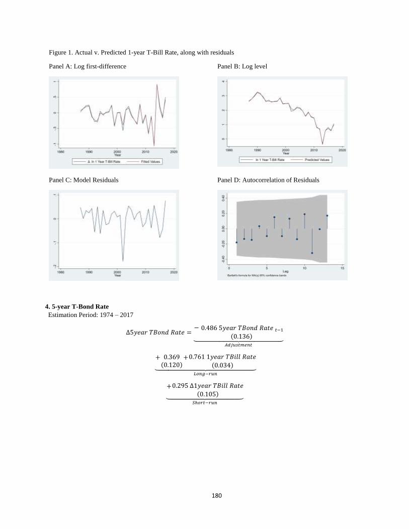
180
Figure 1. Actual v. Predicted 1-year T-Bill Rate, along with residuals
Panel A: Log first-difference Panel B: Log level
Panel C: Model Residuals Panel D: Autocorrelation of Residuals
4. 5-year T-Bond Rate
Estimation Period: 1974 – 2017
∆5𝑦𝑒𝑎𝑟 𝑇𝐵𝑜𝑛𝑑 𝑅𝑎𝑡𝑒 =− 0.486 5𝑦𝑒𝑎𝑟 𝑇𝐵𝑜𝑛𝑑 𝑅𝑎𝑡𝑒 𝑡−1
(0.136)⏟ 𝐴𝑑𝑗𝑢𝑠𝑡𝑚𝑒𝑛𝑡
+ 0.369(0.120)
+0.761 1𝑦𝑒𝑎𝑟 𝑇𝐵𝑖𝑙𝑙 𝑅𝑎𝑡𝑒(0.034)⏟
𝐿𝑜𝑛𝑔−𝑟𝑢𝑛
+0.295 ∆1𝑦𝑒𝑎𝑟 𝑇𝐵𝑖𝑙𝑙 𝑅𝑎𝑡𝑒(0.105)⏟
𝑆ℎ𝑜𝑟𝑡−𝑟𝑢𝑛
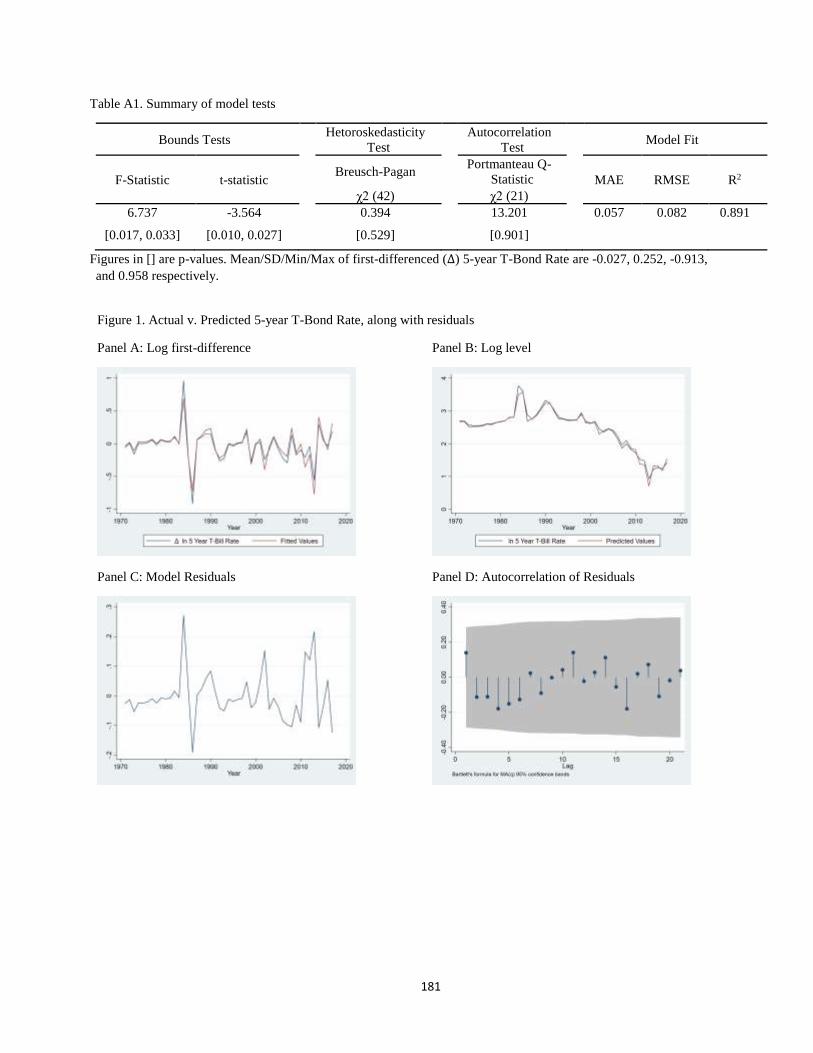
181
Table A1. Summary of model tests
Bounds Tests Hetoroskedasticity
Test Autocorrelation
Test Model Fit
F-Statistic t-statistic Breusch-Pagan Portmanteau Q-
Statistic MAE RMSE R2
χ2 (42) χ2 (21)
6.737 -3.564 0.394 13.201 0.057 0.082 0.891
[0.017, 0.033] [0.010, 0.027] [0.529] [0.901]
Figures in [] are p-values. Mean/SD/Min/Max of first-differenced (∆) 5-year T-Bond Rate are -0.027, 0.252, -0.913,
and 0.958 respectively.
Figure 1. Actual v. Predicted 5-year T-Bond Rate, along with residuals
Panel A: Log first-difference Panel B: Log level
Panel C: Model Residuals Panel D: Autocorrelation of Residuals
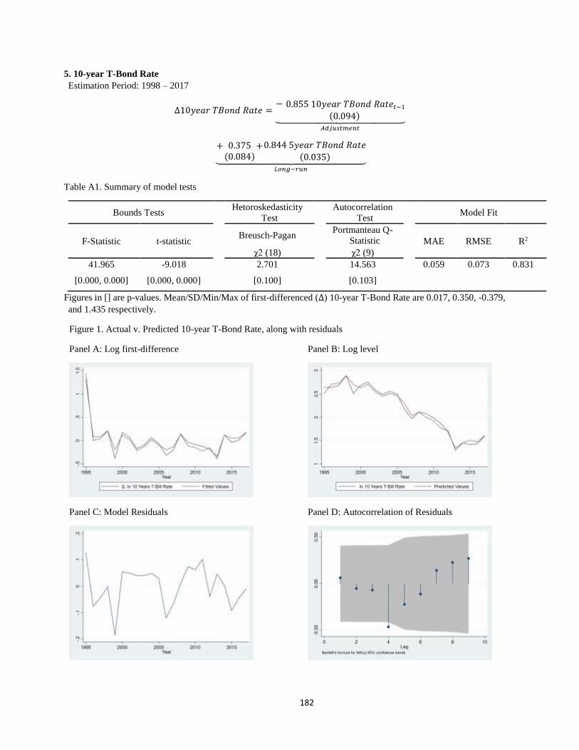
182
5. 10-year T-Bond Rate
Estimation Period: 1998 – 2017
∆10𝑦𝑒𝑎𝑟 𝑇𝐵𝑜𝑛𝑑 𝑅𝑎𝑡𝑒 =− 0.855 10𝑦𝑒𝑎𝑟 𝑇𝐵𝑜𝑛𝑑 𝑅𝑎𝑡𝑒𝑡−1
(0.094)⏟ 𝐴𝑑𝑗𝑢𝑠𝑡𝑚𝑒𝑛𝑡
+ 0.375(0.084)
+0.844 5𝑦𝑒𝑎𝑟 𝑇𝐵𝑜𝑛𝑑 𝑅𝑎𝑡𝑒(0.035)⏟
𝐿𝑜𝑛𝑔−𝑟𝑢𝑛
Table A1. Summary of model tests
Bounds Tests Hetoroskedasticity
Test Autocorrelation
Test Model Fit
F-Statistic t-statistic Breusch-Pagan Portmanteau Q-
Statistic MAE RMSE R2
χ2 (18) χ2 (9)
41.965 -9.018 2.701 14.563 0.059 0.073 0.831
[0.000, 0.000] [0.000, 0.000] [0.100] [0.103]
Figures in [] are p-values. Mean/SD/Min/Max of first-differenced (∆) 10-year T-Bond Rate are 0.017, 0.350, -0.379,
and 1.435 respectively.
Figure 1. Actual v. Predicted 10-year T-Bond Rate, along with residuals
Panel A: Log first-difference Panel B: Log level
Panel C: Model Residuals Panel D: Autocorrelation of Residuals
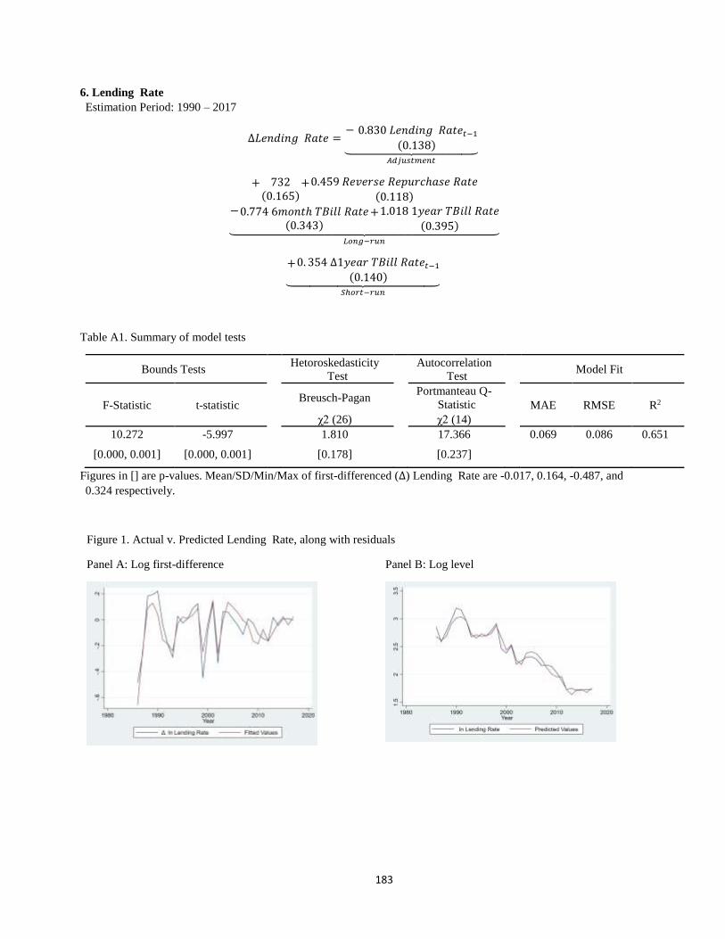
183
6. Lending Rate
Estimation Period: 1990 – 2017
∆𝐿𝑒𝑛𝑑𝑖𝑛𝑔 𝑅𝑎𝑡𝑒 =− 0.830 𝐿𝑒𝑛𝑑𝑖𝑛𝑔 𝑅𝑎𝑡𝑒𝑡−1
(0.138)⏟ 𝐴𝑑𝑗𝑢𝑠𝑡𝑚𝑒𝑛𝑡
+ 732(0.165)
+0.459 𝑅𝑒𝑣𝑒𝑟𝑠𝑒 𝑅𝑒𝑝𝑢𝑟𝑐ℎ𝑎𝑠𝑒 𝑅𝑎𝑡𝑒(0.118)
−0.774 6𝑚𝑜𝑛𝑡ℎ 𝑇𝐵𝑖𝑙𝑙 𝑅𝑎𝑡𝑒(0.343)
+1.018 1𝑦𝑒𝑎𝑟 𝑇𝐵𝑖𝑙𝑙 𝑅𝑎𝑡𝑒(0.395)⏟
𝐿𝑜𝑛𝑔−𝑟𝑢𝑛
+0. 354 ∆1𝑦𝑒𝑎𝑟 𝑇𝐵𝑖𝑙𝑙 𝑅𝑎𝑡𝑒𝑡−1(0.140)⏟
𝑆ℎ𝑜𝑟𝑡−𝑟𝑢𝑛
Table A1. Summary of model tests
Bounds Tests Hetoroskedasticity
Test Autocorrelation
Test Model Fit
F-Statistic t-statistic Breusch-Pagan Portmanteau Q-
Statistic MAE RMSE R2
χ2 (26) χ2 (14)
10.272 -5.997 1.810 17.366 0.069 0.086 0.651
[0.000, 0.001] [0.000, 0.001] [0.178] [0.237]
Figures in [] are p-values. Mean/SD/Min/Max of first-differenced (∆) Lending Rate are -0.017, 0.164, -0.487, and
0.324 respectively.
Figure 1. Actual v. Predicted Lending Rate, along with residuals
Panel A: Log first-difference Panel B: Log level

184
Panel C: Model Residuals Panel D: Autocorrelation of Residuals
7. Time Deposit Rate
Estimation Period: 1990 – 2017
∆𝑇𝑖𝑚𝑒 𝐷𝑒𝑝𝑜𝑠𝑖𝑡 𝑅𝑎𝑡𝑒 =−0.549 𝑇𝑖𝑚𝑒 𝐷𝑒𝑝𝑜𝑠𝑖𝑡 𝑅𝑎𝑡𝑒𝑡−1
(0.106)⏟ 𝐴𝑑𝑗𝑢𝑠𝑡𝑚𝑒𝑛𝑡
− 0.210(0.198)
+0.519 𝑅𝑒𝑣𝑒𝑟𝑠𝑒 𝑅𝑒𝑝𝑢𝑟𝑐ℎ𝑎𝑠𝑒 𝑅𝑎𝑡𝑒(0.286)
+0.560 91𝑑𝑎𝑦 𝑇𝐵𝑖𝑙𝑙 𝑅𝑎𝑡𝑒(0.159)⏟
𝐿𝑜𝑛𝑔−𝑟𝑢𝑛
Table A1. Summary of model tests
Bounds Tests Hetoroskedasticity
Test Autocorrelation
Test Model Fit
F-Statistic t-statistic Breusch-Pagan Portmanteau Q-
Statistic MAE RMSE R2
χ2 (26) χ2 (14)
13.715 -5.148 1.008 19.652 0.123 0.152 0.631
[0.000, 0.000] [0.000, 0.002] [0.315] [0.141]
Figures in [] are p-values. Mean/SD/Min/Max of first-differenced (∆) Time Deposit Rate are -0.024, 0.209, -0.695,
and 0.457 respectively.
Figure 1. Actual v. Predicted Time Deposit Rate, along with residuals
Panel A: Log first-difference Panel B: Log level

185
Panel C: Model Residuals Panel D: Autocorrelation of Residuals
8. Savings Interest Rate
Estimation Period: 1990 – 2017
∆𝑆𝑎𝑣𝑖𝑛𝑔𝑠 𝐼𝑛𝑡𝑒𝑟𝑒𝑠𝑡 𝑅𝑎𝑡𝑒 =−0.419 𝑆𝑎𝑣𝑖𝑛𝑔𝑠 𝐼𝑛𝑡𝑒𝑟𝑒𝑠𝑡 𝑅𝑎𝑡𝑒𝑡−1
(0.094)⏟ 𝐴𝑑𝑗𝑢𝑠𝑡𝑚𝑒𝑛𝑡
− 1.145(0.214)
+1.934 𝑅𝑒𝑣𝑒𝑟𝑠𝑒 𝑅𝑒𝑝𝑢𝑟𝑐ℎ𝑎𝑠𝑒 𝑅𝑎𝑡𝑒(0.160)⏟
𝐿𝑜𝑛𝑔−𝑟𝑢𝑛
Table A1. Summary of model tests
Bounds Tests Hetoroskedasticity
Test Autocorrelation
Test Model Fit
F-Statistic t-statistic Breusch-Pagan Portmanteau Q-
Statistic MAE RMSE R2
χ2 (26) χ2 (14)
12.795 -4.438 0.169 18.356 0.151 0.200 0.505
[0.001, 0.002] [0.002, 0.005] [0.680] [0.191]
Figures in [] are p-values. Mean/SD/Min/Max of first-differenced (∆) Savings Interest Rate are -0.016, 0.209, -0.573,
and 0.560 respectively.
Figure 1. Actual v. Predicted Savings Interest Rate, along with residuals
Panel A: Log first-difference Panel B: Log level

186
Panel C: Model Residuals Panel D: Autocorrelation of Residuals
9. Narrow Money
Estimation Period: 1989 – 2017
∆𝑁𝑎𝑟𝑟𝑜𝑤 𝑀𝑜𝑛𝑒𝑦 =−0.884 𝑁𝑎𝑟𝑟𝑜𝑤 𝑀𝑜𝑛𝑒𝑦𝑡−1
(0.154)⏟ 𝐴𝑑𝑗𝑢𝑠𝑡𝑚𝑒𝑛𝑡
− 6.217(1.262)
+1.458 𝐺𝐷𝑃,𝑁𝑜𝑚𝑖𝑛𝑎𝑙(0.037)
−0.137 𝑆𝑎𝑣𝑖𝑛𝑔𝑠 𝐼𝑛𝑡𝑒𝑟𝑒𝑠𝑡 𝑅𝑎𝑡𝑒
(0.024)−0.214 𝐺𝑜𝑙𝑑 𝑃𝑟𝑖𝑐𝑒 𝑃𝐻𝑃
(0.055)−0.268 𝑈𝑆𝐷 𝑁𝑜𝑚𝑖𝑛𝑎𝑙 𝐸𝑥𝑐ℎ𝑎𝑛𝑔𝑒 𝑅𝑎𝑡𝑒
(0.071)⏟ 𝐿𝑜𝑛𝑔−𝑟𝑢𝑛
−0.108 ∆𝑁𝑎𝑟𝑟𝑜𝑤 𝑀𝑜𝑛𝑒𝑦𝑡−1(0.143)
+0.400 ∆𝑁𝑎𝑟𝑟𝑜𝑤 𝑀𝑜𝑛𝑒𝑦𝑡−2(0.171)
+0.157 ∆𝐺𝑜𝑙𝑑 𝑃𝑟𝑖𝑐𝑒 𝑃𝐻𝑃(0.050)
+0.247 ∆𝑈𝑆𝐷 𝑁𝑜𝑚𝑖𝑛𝑎𝑙 𝐸𝑥𝑐ℎ𝑎𝑛𝑔𝑒 𝑅𝑎𝑡𝑒
(0.080)+0.140 ∆𝑈𝑆𝐷 𝑁𝑜𝑚𝑖𝑛𝑎𝑙 𝐸𝑥𝑐ℎ𝑎𝑛𝑔𝑒 𝑅𝑎𝑡𝑒𝑡−1
(0.064)
+0.238 ∆𝑈𝑆𝐷 𝑁𝑜𝑚𝑖𝑛𝑎𝑙 𝐸𝑥𝑐ℎ𝑎𝑛𝑔𝑒 𝑅𝑎𝑡𝑒𝑡−2(0.078)⏟
𝑆ℎ𝑜𝑟𝑡−𝑟𝑢𝑛
Table A1. Summary of model tests
Bounds Tests Hetoroskedasticity
Test Autocorrelation
Test Model Fit
F-Statistic t-statistic Breusch-Pagan Portmanteau Q-
Statistic MAE RMSE R2
χ2 (27) χ2 (13)
11.415 -5.715 0.369 10.244 0.018 0.024 0.794
[0.000, 0.001] [0.000, 0.004] [0.543] [0.673]
Figures in [] are p-values. Mean/SD/Min/Max of first-differenced (∆) Narrow Money are 0.135, 0.056, -0.072, and
0.262 respectively.
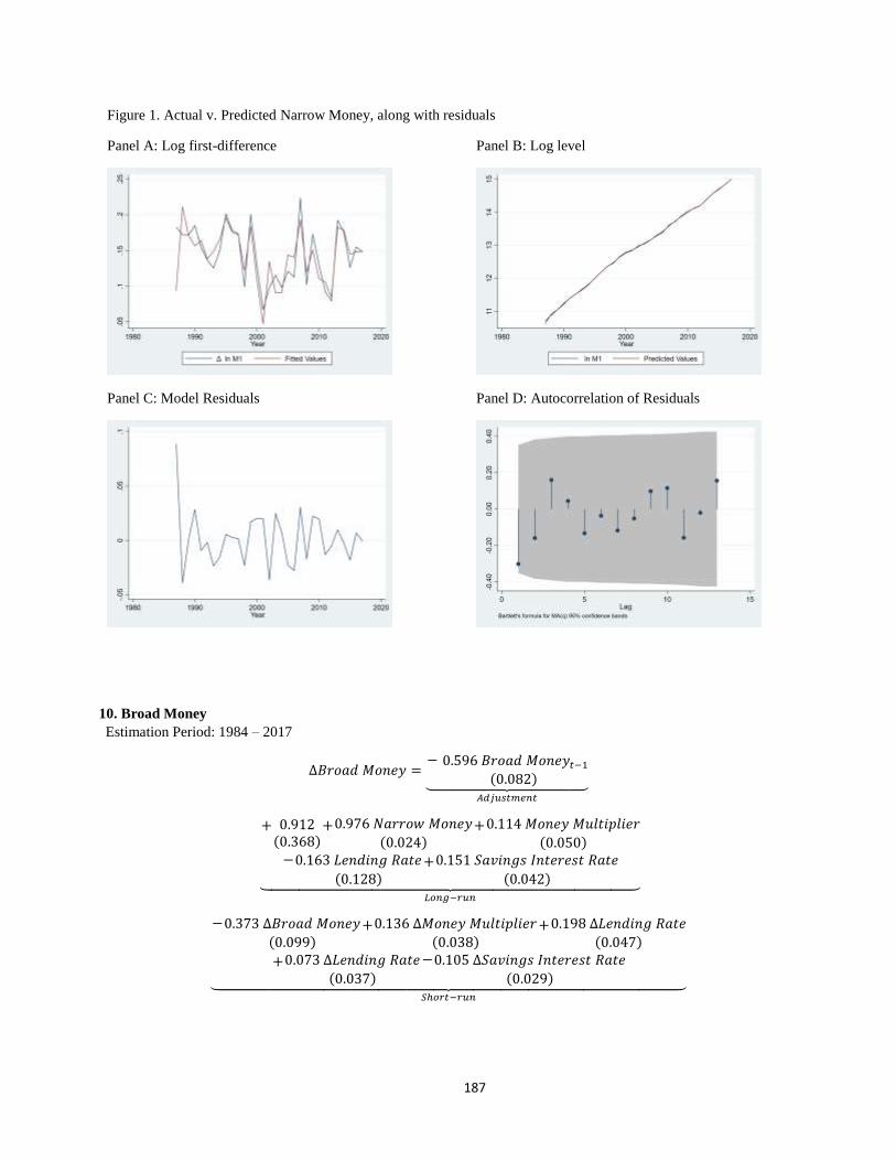
187
Figure 1. Actual v. Predicted Narrow Money, along with residuals
Panel A: Log first-difference Panel B: Log level
Panel C: Model Residuals Panel D: Autocorrelation of Residuals
10. Broad Money
Estimation Period: 1984 – 2017
∆𝐵𝑟𝑜𝑎𝑑 𝑀𝑜𝑛𝑒𝑦 =− 0.596 𝐵𝑟𝑜𝑎𝑑 𝑀𝑜𝑛𝑒𝑦𝑡−1
(0.082)⏟ 𝐴𝑑𝑗𝑢𝑠𝑡𝑚𝑒𝑛𝑡
+ 0.912(0.368)
+0.976 𝑁𝑎𝑟𝑟𝑜𝑤 𝑀𝑜𝑛𝑒𝑦
(0.024)+0.114 𝑀𝑜𝑛𝑒𝑦 𝑀𝑢𝑙𝑡𝑖𝑝𝑙𝑖𝑒𝑟
(0.050)−0.163 𝐿𝑒𝑛𝑑𝑖𝑛𝑔 𝑅𝑎𝑡𝑒
(0.128)+0.151 𝑆𝑎𝑣𝑖𝑛𝑔𝑠 𝐼𝑛𝑡𝑒𝑟𝑒𝑠𝑡 𝑅𝑎𝑡𝑒
(0.042)⏟ 𝐿𝑜𝑛𝑔−𝑟𝑢𝑛
−0.373 ∆𝐵𝑟𝑜𝑎𝑑 𝑀𝑜𝑛𝑒𝑦
(0.099)+0.136 ∆𝑀𝑜𝑛𝑒𝑦 𝑀𝑢𝑙𝑡𝑖𝑝𝑙𝑖𝑒𝑟
(0.038)+0.198 ∆𝐿𝑒𝑛𝑑𝑖𝑛𝑔 𝑅𝑎𝑡𝑒
(0.047)
+0.073 ∆𝐿𝑒𝑛𝑑𝑖𝑛𝑔 𝑅𝑎𝑡𝑒
(0.037)
−0.105 ∆𝑆𝑎𝑣𝑖𝑛𝑔𝑠 𝐼𝑛𝑡𝑒𝑟𝑒𝑠𝑡 𝑅𝑎𝑡𝑒
(0.029)⏟ 𝑆ℎ𝑜𝑟𝑡−𝑟𝑢𝑛

188
Table A1. Summary of model tests
Bounds Tests Hetoroskedasticity
Test Autocorrelation
Test Model Fit
F-Statistic t-statistic Breusch-Pagan Portmanteau Q-
Statistic MAE RMSE R2
χ2 (32) χ2 (16)
11.470 -7.199 0.336 11.383 0.020 0.031 0.870
[0.000, 0.000] [0.000, 0.000] [0.561] [0.785]
Figures in [] are p-values. Mean/SD/Min/Max of first-differenced (∆) Broad Money are 0.143, 0.068, 0.049, and
0.360 respectively.
Figure 1. Actual v. Predicted Broad Money, along with residuals
Panel A: Log first-difference Panel B: Log level
Panel C: Model Residuals Panel D: Autocorrelation of Residuals
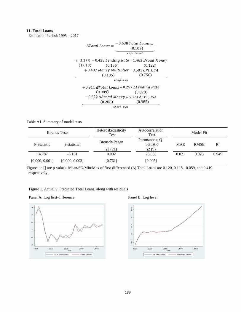
189
11. Total Loans
Estimation Period: 1995 – 2017
∆𝑇𝑜𝑡𝑎𝑙 𝐿𝑜𝑎𝑛𝑠 =−0.638 𝑇𝑜𝑡𝑎𝑙 𝐿𝑜𝑎𝑛𝑠𝑡−1
(0.103)⏟ 𝐴𝑑𝑗𝑢𝑠𝑡𝑚𝑒𝑛𝑡
+ 5.238(1.613)
−0.435 𝐿𝑒𝑛𝑑𝑖𝑛𝑔 𝑅𝑎𝑡𝑒
(0.155)+1.463 𝐵𝑟𝑜𝑎𝑑 𝑀𝑜𝑛𝑒𝑦
(0.122)
+0.497 𝑀𝑜𝑛𝑒𝑦 𝑀𝑢𝑙𝑡𝑖𝑝𝑙𝑖𝑒𝑟
(0.135)
−3.501 𝐶𝑃𝐼, 𝑈𝑆𝐴(0.756)⏟
𝐿𝑜𝑛𝑔−𝑟𝑢𝑛
+0.911 ∆𝑇𝑜𝑡𝑎𝑙 𝐿𝑜𝑎𝑛𝑠(0.089)
+0.257 ∆𝐿𝑒𝑛𝑑𝑖𝑛𝑔 𝑅𝑎𝑡𝑒
(0.070)−0.522 ∆𝐵𝑟𝑜𝑎𝑑 𝑀𝑜𝑛𝑒𝑦
(0.206)+5.373 ∆𝐶𝑃𝐼, 𝑈𝑆𝐴
(0.985)⏟ 𝑆ℎ𝑜𝑟𝑡−𝑟𝑢𝑛
Table A1. Summary of model tests
Bounds Tests Hetoroskedasticity
Test Autocorrelation
Test Model Fit
F-Statistic t-statistic Breusch-Pagan Portmanteau Q-
Statistic MAE RMSE R2
χ2 (21) χ2 (9)
14.787 -6.161 0.092 23.583 0.021 0.025 0.949
[0.000, 0.001] [0.000, 0.003] [0.761] [0.005]
Figures in [] are p-values. Mean/SD/Min/Max of first-differenced (∆) Total Loans are 0.120, 0.115, -0.059, and 0.419
respectively.
Figure 1. Actual v. Predicted Total Loans, along with residuals
Panel A: Log first-difference Panel B: Log level
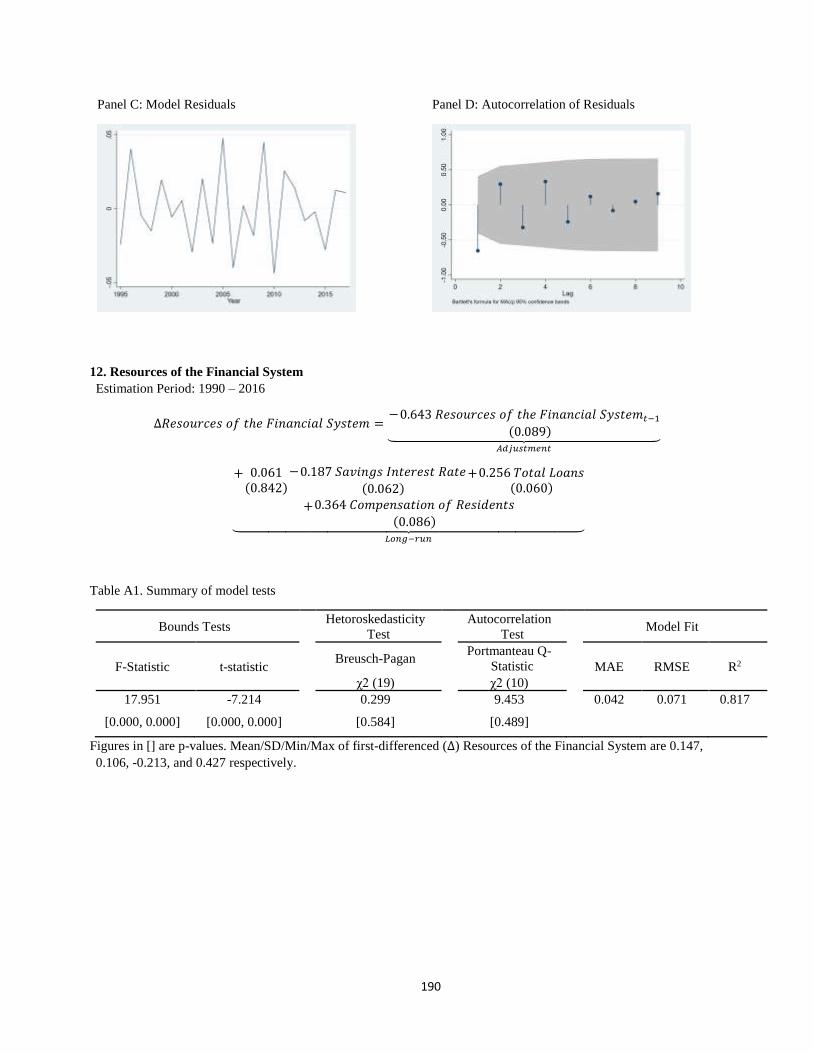
190
Panel C: Model Residuals Panel D: Autocorrelation of Residuals
12. Resources of the Financial System
Estimation Period: 1990 – 2016
∆𝑅𝑒𝑠𝑜𝑢𝑟𝑐𝑒𝑠 𝑜𝑓 𝑡ℎ𝑒 𝐹𝑖𝑛𝑎𝑛𝑐𝑖𝑎𝑙 𝑆𝑦𝑠𝑡𝑒𝑚 =−0.643 𝑅𝑒𝑠𝑜𝑢𝑟𝑐𝑒𝑠 𝑜𝑓 𝑡ℎ𝑒 𝐹𝑖𝑛𝑎𝑛𝑐𝑖𝑎𝑙 𝑆𝑦𝑠𝑡𝑒𝑚𝑡−1
(0.089)⏟ 𝐴𝑑𝑗𝑢𝑠𝑡𝑚𝑒𝑛𝑡
+ 0.061(0.842)
−0.187 𝑆𝑎𝑣𝑖𝑛𝑔𝑠 𝐼𝑛𝑡𝑒𝑟𝑒𝑠𝑡 𝑅𝑎𝑡𝑒
(0.062)+0.256 𝑇𝑜𝑡𝑎𝑙 𝐿𝑜𝑎𝑛𝑠
(0.060)
+0.364 𝐶𝑜𝑚𝑝𝑒𝑛𝑠𝑎𝑡𝑖𝑜𝑛 𝑜𝑓 𝑅𝑒𝑠𝑖𝑑𝑒𝑛𝑡𝑠
(0.086)⏟ 𝐿𝑜𝑛𝑔−𝑟𝑢𝑛
Table A1. Summary of model tests
Bounds Tests Hetoroskedasticity
Test Autocorrelation
Test Model Fit
F-Statistic t-statistic Breusch-Pagan Portmanteau Q-
Statistic MAE RMSE R2
χ2 (19) χ2 (10)
17.951 -7.214 0.299 9.453 0.042 0.071 0.817
[0.000, 0.000] [0.000, 0.000] [0.584] [0.489]
Figures in [] are p-values. Mean/SD/Min/Max of first-differenced (∆) Resources of the Financial System are 0.147,
0.106, -0.213, and 0.427 respectively.

191
Figure 1. Actual v. Predicted Resources of the Financial System, along with residuals
Panel A: Log first-difference Panel B: Log level
Panel C: Model Residuals Panel D: Autocorrelation of Residuals
13. Cash Remittances
Estimation Period: 1974 – 2016
∆𝐶𝑎𝑠ℎ 𝑅𝑒𝑚𝑖𝑡𝑡𝑎𝑛𝑐𝑒𝑠 =−0.275 𝐶𝑎𝑠ℎ 𝑅𝑒𝑚𝑖𝑡𝑡𝑎𝑛𝑐𝑒𝑠𝑡−1
(0.073)⏟ 𝐴𝑑𝑗𝑢𝑠𝑡𝑚𝑒𝑛𝑡
+ 2.197(0.446)
+1.112 𝐶𝑃𝐼, 𝑃ℎ𝑖𝑙𝑖𝑝𝑝𝑖𝑛𝑒𝑠(0.144)
−1.419 𝑈𝑛𝑒𝑚𝑝𝑙𝑜𝑦𝑚𝑒𝑛𝑡 𝑅𝑎𝑡𝑒(0.388)⏟
𝐿𝑜𝑛𝑔−𝑟𝑢𝑛
+0.218 ∆𝐶𝑎𝑠ℎ 𝑅𝑒𝑚𝑖𝑡𝑡𝑎𝑛𝑐𝑒𝑠𝑡−1(0.052)
−0.203 ∆𝐶𝑎𝑠ℎ 𝑅𝑒𝑚𝑖𝑡𝑡𝑎𝑛𝑐𝑒𝑠𝑡−2(0.053)
−1.116 ∆𝐶𝑃𝐼, 𝑃ℎ𝑖𝑙𝑖𝑝𝑝𝑖𝑛𝑒𝑠(0.312)
−0.119 ∆𝐶𝑃𝐼, 𝑃ℎ𝑖𝑙𝑖𝑝𝑝𝑖𝑛𝑒𝑠𝑡−1(0.305)
−0.911 ∆𝐶𝑃𝐼, 𝑃ℎ𝑖𝑙𝑖𝑝𝑝𝑖𝑛𝑒𝑠𝑡−2(0.308)
+0.535 ∆𝑈𝑛𝑒𝑚𝑝𝑙𝑜𝑦𝑚𝑒𝑛𝑡 𝑅𝑎𝑡𝑒(0.206)⏟
𝑆ℎ𝑜𝑟𝑡−𝑟𝑢𝑛

192
Table A1. Summary of model tests
Bounds Tests Hetoroskedasticity
Test Autocorrelation
Test Model Fit
F-Statistic t-statistic Breusch-Pagan Portmanteau Q-
Statistic MAE RMSE R2
χ2 (41) χ2 (20)
11.358 -3.739 0.000 5.600 0.100 0.194 0.709
[0.000, 0.036] [0.007, 0.036] [0.989] [0.999]
Figures in [] are p-values. Mean/SD/Min/Max of first-differenced (∆) Cash Remittances are 0.168, 0.397, -0.693, and
2.397 respectively.
Figure 1. Actual v. Predicted Cash Remittances, along with residuals
Panel A: Log first-difference Panel B: Log level
Panel C: Model Residuals Panel D: Autocorrelation of Residuals
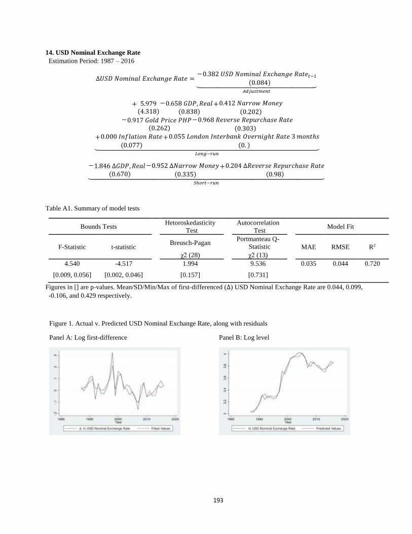
193
14. USD Nominal Exchange Rate
Estimation Period: 1987 – 2016
∆𝑈𝑆𝐷 𝑁𝑜𝑚𝑖𝑛𝑎𝑙 𝐸𝑥𝑐ℎ𝑎𝑛𝑔𝑒 𝑅𝑎𝑡𝑒 =−0.382 𝑈𝑆𝐷 𝑁𝑜𝑚𝑖𝑛𝑎𝑙 𝐸𝑥𝑐ℎ𝑎𝑛𝑔𝑒 𝑅𝑎𝑡𝑒𝑡−1
(0.084)⏟ 𝐴𝑑𝑗𝑢𝑠𝑡𝑚𝑒𝑛𝑡
+ 5.979(4.318)
−0.658 𝐺𝐷𝑃, 𝑅𝑒𝑎𝑙(0.838)
+0.412 𝑁𝑎𝑟𝑟𝑜𝑤 𝑀𝑜𝑛𝑒𝑦
(0.202)−0.917 𝐺𝑜𝑙𝑑 𝑃𝑟𝑖𝑐𝑒 𝑃𝐻𝑃
(0.262)−0.968 𝑅𝑒𝑣𝑒𝑟𝑠𝑒 𝑅𝑒𝑝𝑢𝑟𝑐ℎ𝑎𝑠𝑒 𝑅𝑎𝑡𝑒
(0.303)
+0.000 𝐼𝑛𝑓𝑙𝑎𝑡𝑖𝑜𝑛 𝑅𝑎𝑡𝑒
(0.077)+0.055 𝐿𝑜𝑛𝑑𝑜𝑛 𝐼𝑛𝑡𝑒𝑟𝑏𝑎𝑛𝑘 𝑂𝑣𝑒𝑟𝑛𝑖𝑔ℎ𝑡 𝑅𝑎𝑡𝑒 3 𝑚𝑜𝑛𝑡ℎ𝑠
(0. )⏟ 𝐿𝑜𝑛𝑔−𝑟𝑢𝑛
−1.846 ∆𝐺𝐷𝑃, 𝑅𝑒𝑎𝑙(0.670)
−0.952 ∆𝑁𝑎𝑟𝑟𝑜𝑤 𝑀𝑜𝑛𝑒𝑦(0.335)
+0.204 ∆𝑅𝑒𝑣𝑒𝑟𝑠𝑒 𝑅𝑒𝑝𝑢𝑟𝑐ℎ𝑎𝑠𝑒 𝑅𝑎𝑡𝑒(0.98)⏟
𝑆ℎ𝑜𝑟𝑡−𝑟𝑢𝑛
Table A1. Summary of model tests
Bounds Tests Hetoroskedasticity
Test Autocorrelation
Test Model Fit
F-Statistic t-statistic Breusch-Pagan Portmanteau Q-
Statistic MAE RMSE R2
χ2 (28) χ2 (13)
4.540 -4.517 1.994 9.536 0.035 0.044 0.720
[0.009, 0.056] [0.002, 0.046] [0.157] [0.731]
Figures in [] are p-values. Mean/SD/Min/Max of first-differenced (∆) USD Nominal Exchange Rate are 0.044, 0.099,
-0.106, and 0.429 respectively.
Figure 1. Actual v. Predicted USD Nominal Exchange Rate, along with residuals
Panel A: Log first-difference Panel B: Log level
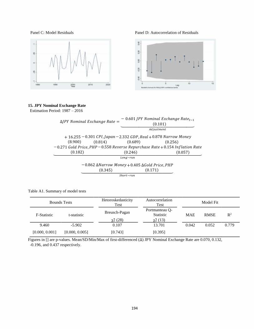
194
Panel C: Model Residuals Panel D: Autocorrelation of Residuals
15. JPY Nominal Exchange Rate
Estimation Period: 1987 – 2016
∆𝐽𝑃𝑌 𝑁𝑜𝑚𝑖𝑛𝑎𝑙 𝐸𝑥𝑐ℎ𝑎𝑛𝑔𝑒 𝑅𝑎𝑡𝑒 =− 0.601 𝐽𝑃𝑌 𝑁𝑜𝑚𝑖𝑛𝑎𝑙 𝐸𝑥𝑐ℎ𝑎𝑛𝑔𝑒 𝑅𝑎𝑡𝑒𝑡−1
(0.101)⏟ 𝐴𝑑𝑗𝑢𝑠𝑡𝑚𝑒𝑛𝑡
+ 16.255(8.900)
−0.301 𝐶𝑃𝐼, 𝐽𝑎𝑝𝑎𝑛
(0.814)
−2.332 𝐺𝐷𝑃, 𝑅𝑒𝑎𝑙(0.689)
+0.878 𝑁𝑎𝑟𝑟𝑜𝑤 𝑀𝑜𝑛𝑒𝑦
(0.256)−0.271 𝐺𝑜𝑙𝑑 𝑃𝑟𝑖𝑐𝑒, 𝑃𝐻𝑃
(0.182)
−0.558 𝑅𝑒𝑣𝑒𝑟𝑠𝑒 𝑅𝑒𝑝𝑢𝑟𝑐ℎ𝑎𝑠𝑒 𝑅𝑎𝑡𝑒(0.246)
+0.154 𝐼𝑛𝑓𝑙𝑎𝑡𝑖𝑜𝑛 𝑅𝑎𝑡𝑒
(0.057)⏟ 𝐿𝑜𝑛𝑔−𝑟𝑢𝑛
−0.862 ∆𝑁𝑎𝑟𝑟𝑜𝑤 𝑀𝑜𝑛𝑒𝑦(0.345)
+0.405 ∆𝐺𝑜𝑙𝑑 𝑃𝑟𝑖𝑐𝑒, 𝑃𝐻𝑃(0.171)⏟
𝑆ℎ𝑜𝑟𝑡−𝑟𝑢𝑛
Table A1. Summary of model tests
Bounds Tests Hetoroskedasticity
Test Autocorrelation
Test Model Fit
F-Statistic t-statistic Breusch-Pagan Portmanteau Q-
Statistic MAE RMSE R2
χ2 (28) χ2 (13)
9.460 -5.902 0.107 13.701 0.042 0.052 0.779
[0.000, 0.001] [0.000, 0.005] [0.743] [0.395]
Figures in [] are p-values. Mean/SD/Min/Max of first-differenced (∆) JPY Nominal Exchange Rate are 0.070, 0.132,
-0.196, and 0.437 respectively.
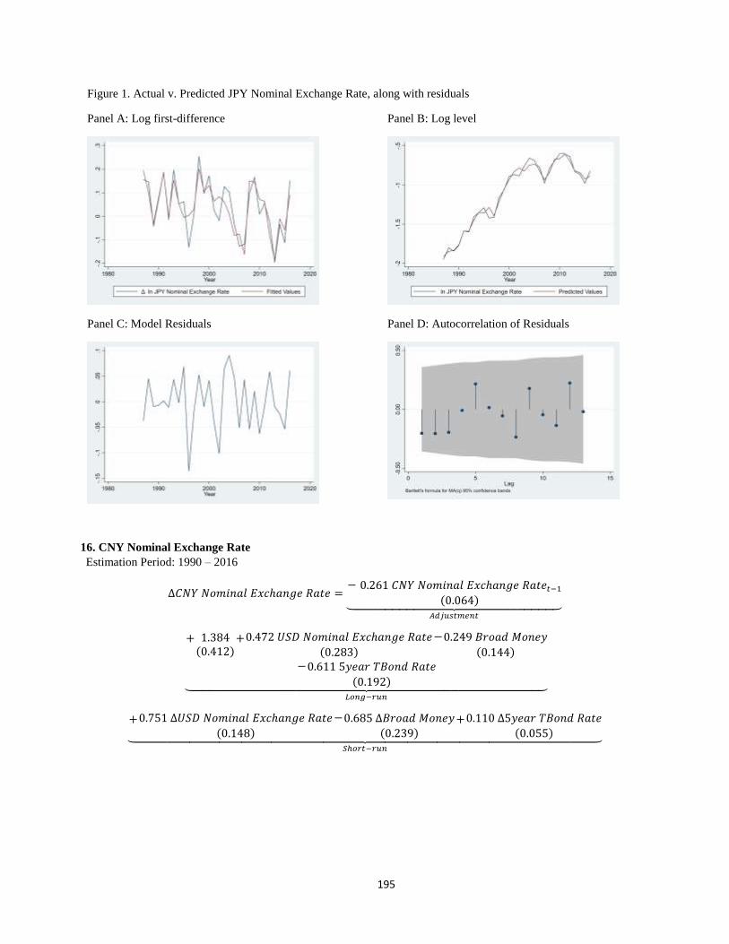
195
Figure 1. Actual v. Predicted JPY Nominal Exchange Rate, along with residuals
Panel A: Log first-difference Panel B: Log level
Panel C: Model Residuals Panel D: Autocorrelation of Residuals
16. CNY Nominal Exchange Rate
Estimation Period: 1990 – 2016
∆𝐶𝑁𝑌 𝑁𝑜𝑚𝑖𝑛𝑎𝑙 𝐸𝑥𝑐ℎ𝑎𝑛𝑔𝑒 𝑅𝑎𝑡𝑒 =− 0.261 𝐶𝑁𝑌 𝑁𝑜𝑚𝑖𝑛𝑎𝑙 𝐸𝑥𝑐ℎ𝑎𝑛𝑔𝑒 𝑅𝑎𝑡𝑒𝑡−1
(0.064)⏟ 𝐴𝑑𝑗𝑢𝑠𝑡𝑚𝑒𝑛𝑡
+ 1.384(0.412)
+0.472 𝑈𝑆𝐷 𝑁𝑜𝑚𝑖𝑛𝑎𝑙 𝐸𝑥𝑐ℎ𝑎𝑛𝑔𝑒 𝑅𝑎𝑡𝑒
(0.283)
−0.249 𝐵𝑟𝑜𝑎𝑑 𝑀𝑜𝑛𝑒𝑦
(0.144)−0.611 5𝑦𝑒𝑎𝑟 𝑇𝐵𝑜𝑛𝑑 𝑅𝑎𝑡𝑒
(0.192)⏟ 𝐿𝑜𝑛𝑔−𝑟𝑢𝑛
+0.751 ∆𝑈𝑆𝐷 𝑁𝑜𝑚𝑖𝑛𝑎𝑙 𝐸𝑥𝑐ℎ𝑎𝑛𝑔𝑒 𝑅𝑎𝑡𝑒
(0.148)
−0.685 ∆𝐵𝑟𝑜𝑎𝑑 𝑀𝑜𝑛𝑒𝑦(0.239)
+0.110 ∆5𝑦𝑒𝑎𝑟 𝑇𝐵𝑜𝑛𝑑 𝑅𝑎𝑡𝑒(0.055)⏟
𝑆ℎ𝑜𝑟𝑡−𝑟𝑢𝑛
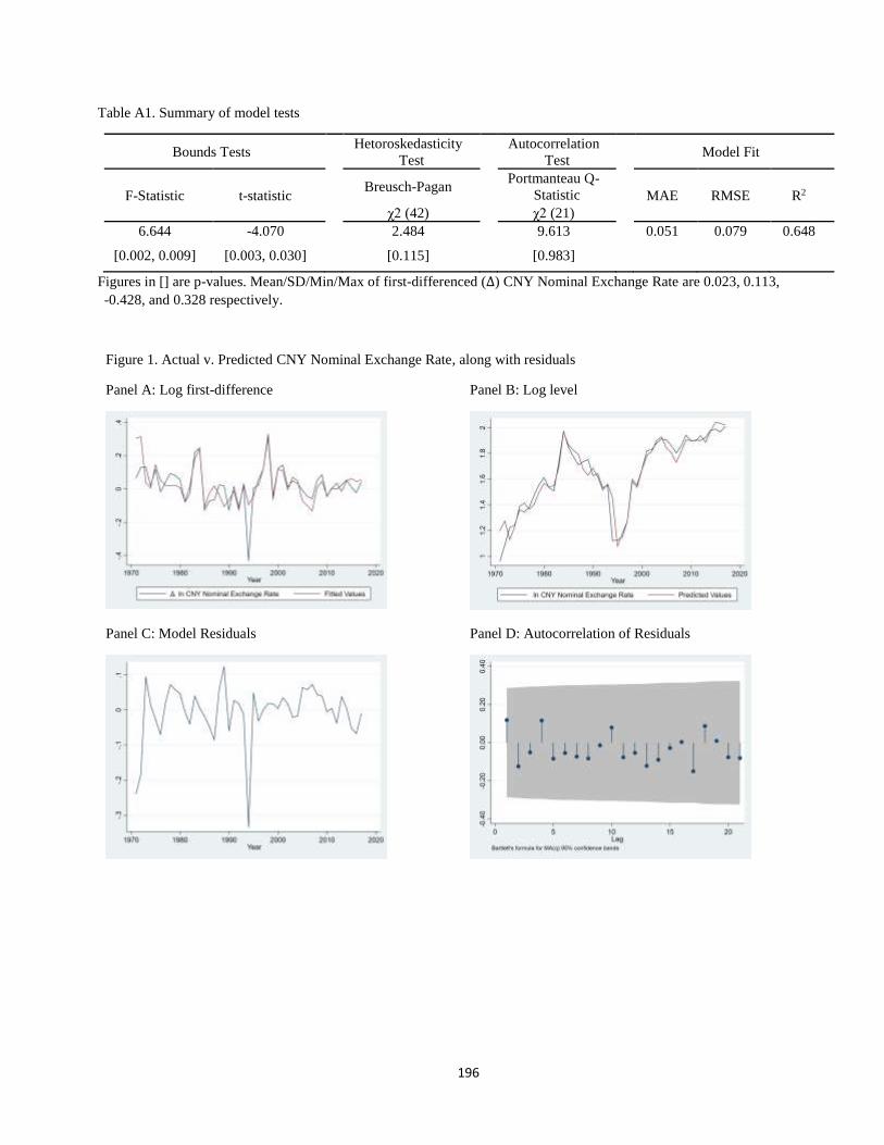
196
Table A1. Summary of model tests
Bounds Tests Hetoroskedasticity
Test Autocorrelation
Test Model Fit
F-Statistic t-statistic Breusch-Pagan Portmanteau Q-
Statistic MAE RMSE R2
χ2 (42) χ2 (21)
6.644 -4.070 2.484 9.613 0.051 0.079 0.648
[0.002, 0.009] [0.003, 0.030] [0.115] [0.983]
Figures in [] are p-values. Mean/SD/Min/Max of first-differenced (∆) CNY Nominal Exchange Rate are 0.023, 0.113,
-0.428, and 0.328 respectively.
Figure 1. Actual v. Predicted CNY Nominal Exchange Rate, along with residuals
Panel A: Log first-difference Panel B: Log level
Panel C: Model Residuals Panel D: Autocorrelation of Residuals

197
17. Money Multiplier
Estimation Period: 1984 – 2017
∆𝑀𝑜𝑛𝑒𝑦 𝑀𝑢𝑙𝑡𝑖𝑝𝑙𝑖𝑒𝑟 =−0.647 𝑀𝑜𝑛𝑒𝑦 𝑀𝑢𝑙𝑡𝑖𝑝𝑙𝑖𝑒𝑟𝑡−1
(0.164)⏟ 𝐴𝑑𝑗𝑢𝑠𝑡𝑚𝑒𝑛𝑡
+ 1.592(0.426)
−0.506 𝑅𝑒𝑠𝑒𝑟𝑣𝑒 𝑅𝑒𝑞𝑢𝑖𝑟𝑒𝑚𝑒𝑛𝑡 𝑅𝑎𝑡𝑖𝑜(0.035)
+0.042 𝑆𝑎𝑣𝑖𝑛𝑔𝑠 𝐼𝑛𝑡𝑒𝑟𝑒𝑠𝑡 𝑅𝑎𝑡𝑒
(0.005)⏟ 𝐿𝑜𝑛𝑔−𝑟𝑢𝑛
−0.159 ∆𝑅𝑒𝑠𝑒𝑟𝑣𝑒 𝑅𝑒𝑞𝑢𝑖𝑟𝑒𝑚𝑒𝑛𝑡 𝑅𝑎𝑡𝑖𝑜(0.080)⏟
𝑆ℎ𝑜𝑟𝑡−𝑟𝑢𝑛
Table A1. Summary of model tests
Bounds Tests Hetoroskedasticity
Test Autocorrelation
Test Model Fit
F-Statistic t-statistic Breusch-Pagan Portmanteau Q-
Statistic MAE RMSE R2
χ2 (32) χ2 (16)
5.577 -3.925 0.013 21.767 0.015 0.017 0.867
[0.015, 0.043] [0.005, 0.027] [0.908] [0.150]
Figures in [] are p-values. Mean/SD/Min/Max of first-differenced (∆) Money Multiplier are -0.001, 0.050, -0.155,
and 0.127 respectively.
Figure 1. Actual v. Predicted Money Multiplier, along with residuals
Panel A: Log first-difference Panel B: Log level
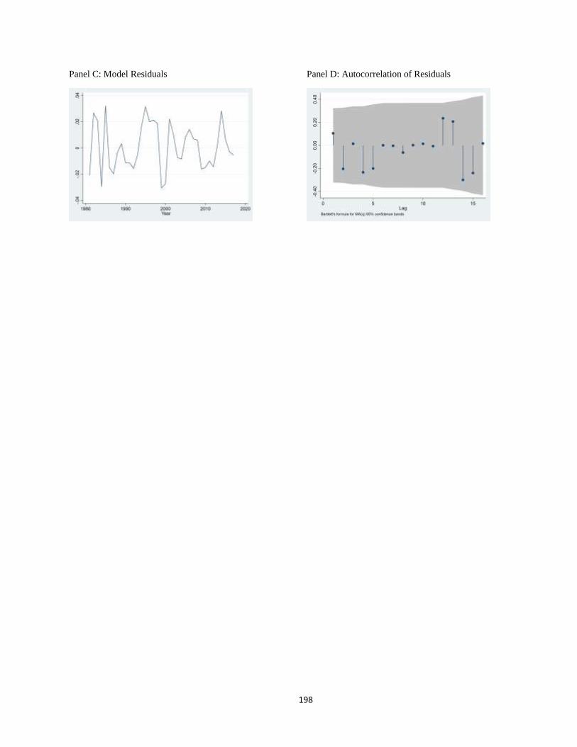
198
Panel C: Model Residuals Panel D: Autocorrelation of Residuals

199
APPENDIX 4: Test of the predictive accuracy
Table 1. Test of the predictive accuracy of forecasts: MAPE
In-sample forecast Out-sample forecast 2002-2016 2017 2018
GDP, real 0.021 0.024 0.029
GDP, nominal 0.011 0.005 0.003
Nominal GDP (exp) 0.022 0.019 0.08
GVA Agriculture, real 0.018 0.017 0.006
GVA Agriculture (demand), real 0.008 0.002 0.012
GVA Construction, real 0.059 0.158 0.129
GVA Electricity and Steam, real 0.041 0.069 0.057
GVA Finance, real 0.031 0.01 0.031
GVA Manufacturing, real 0.051 0.078 0.09
GVA Mining, real 0.093 0.057 0.124
GVA Mining, nominal 0.096 0.102 0.148
GVA Other Services, real 0.029 0.031 0.072
GVA Real Estate, real 0.016 0.034 0.067
GVA Trade, real 0.044 0.072 0.088
GVA Transportation, real 0.039 0.088 0.186
GVA Water, real 0.049 0.016 0.018
IPIN GVA Construction 0.052 0.011 0.037
IPIN GVA Electricity and Steam 0.026 0.027 0.072
IPIN GVA Finance 0.03 0.032 0.095
IPIN GVA Manufacturing 0.07 0.031 0.041
IPIN GVA Mining 0.073 0.047 0.027
IPIN GVA Other Services 0.038 0.019 0.035
IPIN GVA Real Estate 0.021 0.024 0.095
IPIN GVA Trade 0.075 0.118 0.156
IPIN GVA Transportation 0.048 0.1 0.114
IPIN GVA Water 0.056 0.016 0.062
HFCE - Alcohol 0.031 0.113 0.435
HFCE - Education 0.031 0.042 0.073
HFCE - Food 0.016 0.015 0.009
HFCE - Medical 0.027 0.085 0.169
HFCE - Housing 0.022 0.125 0.078
HFCE - Non-Alcoholic 0.045 0.084 0.222
HFCE - Miscellaneous 0.017 0.01 0.03
HFCE - Tobacco 0.039 0.014 0.034
HFCE - Transportation and Communication 0.031 0.002 0.004
HFCE - Utilities 0.042 0.047 0.086
IPIN HFCE - Alcohol 0.022 0.072 0.203
IPIN HFCE - Education 0.013 0.03 0.104
IPIN HFCE - Food 0.016 0.033 0.014
IPIN HFCE - Medical 0.026 0.145 0.285
IPIN HFCE - Housing 0.032 0.07 0.065
IPIN HFCE - Non-Alcoholic 0.014 0.005 0.012
IPIN HFCE - Miscellaneous 0.078 0.005 0.012
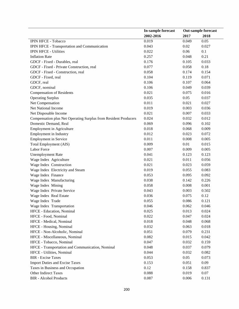
200
In-sample forecast Out-sample forecast 2002-2016 2017 2018
IPIN HFCE - Tobacco 0.019 0.049 0.05
IPIN HFCE - Transportation and Communication 0.043 0.02 0.027
IPIN HFCE - Utilities 0.022 0.06 0.1
Inflation Rate 0.257 0.048 0.21
GDCF - Fixed - Durables, real 0.176 0.105 0.033
GDCF - Fixed - Private Construction, real 0.077 0.058 0.18
GDCF - Fixed - Construction, real 0.058 0.174 0.154
GDCF - Fixed, real 0.104 0.119 0.071
GDCF, real 0.106 0.107 0.064
GDCF, nominal 0.106 0.049 0.039
Compensation of Residents 0.021 0.075 0.016
Operating Surplus 0.035 0.05 0.037
Net Compensation 0.011 0.021 0.027
Net National Income 0.019 0.003 0.036
Net Disposable Income 0.021 0.007 0.033
Compensation plus Net Operating Surplus from Resident Producers 0.024 0.032 0.012
Domestic Demand, Real 0.069 0.096 0.102
Employment in Agriculture 0.018 0.068 0.009
Employment in Industry 0.012 0.023 0.072
Employment in Service 0.011 0.008 0.005
Total Employment (AIS) 0.009 0.01 0.015
Labor Force 0.007 0.009 0.005
Unemployment Rate 0.041 0.123 0.123
Wage Index Agriculture 0.021 0.011 0.056
Wage Index Construction 0.021 0.023 0.059
Wage Index Electricity and Steam 0.019 0.055 0.083
Wage Index Finance 0.053 0.095 0.092
Wage Index Manufacturing 0.038 0.142 0.226
Wage Index Mining 0.058 0.008 0.001
Wage Index Private Service 0.043 0.003 0.502
Wage Index Real Estate 0.036 0.075 0.12
Wage Index Trade 0.055 0.086 0.121
Wage Index Transportation 0.046 0.062 0.046
HFCE - Education, Nominal 0.025 0.013 0.024
HFCE - Food, Nominal 0.022 0.047 0.024
HFCE - Medical, Nominal 0.018 0.048 0.068
HFCE - Housing, Nominal 0.032 0.063 0.018
HFCE - Non-Alcoholic, Nominal 0.051 0.079 0.231
HFCE - Miscellaneous, Nominal 0.082 0.015 0.042
HFCE - Tobacco, Nominal 0.047 0.032 0.159
HFCE - Transportation and Communication, Nominal 0.048 0.037 0.079
HFCE - Utilities, Nominal 0.044 0.032 0.082
BIR - Excise Taxes 0.053 0.05 0.073
Import Duties and Excise Taxes 0.153 0.051 0.09
Taxes in Business and Occupation 0.12 0.158 0.837
Other Indirect Taxes 0.088 0.019 0.07
BIR - Alcohol Products 0.087 0.006 0.131

201
In-sample forecast Out-sample forecast 2002-2016 2017 2018
BIR - Tobacco Products (including inspection fees) 0.07 0.07 0.285
BIR - Petroleum Products 0.042 0.032 0.024
BIR - Mineral Products 0.084 0.099 1.554
Excise Tax on Domestic Product 0.224 0.086 0.21
Income Tax on Business 0.143 0.067 0.202
Income Tax on Individual 0.164 0.093 0.589
Other Direct Taxes 0.236 0.066 0.922
Compulsory fees and fines 0.175 0.061 0.158
Govt property income 0.095 0.06 0.153
Social security contributions 0.067 0.054 0.24
Govt property expenditure 0.099 0.088 0.117
Social security benefits 0.059 0.151 0.236
Total Indirect Taxes 0.139 0.11 0.364
Total Direct Taxes 0.1 0.078 0.181
Total Taxes 0.054 0.027 0.357
Total Govt Income 0.047 0.008 0.23
Total Govt Expenditure 0.021 0.002 0.008
Total Govt Savings 0.291 0.072 2.036
Total Govt Surplus 0.63 0.125 2.149
Total Govt Debt 0.0523 0.0146 0.3634
IPIN Agricultural Imports 0.067 0.227 0.491
IPIN Fuel Imports 0.079 0.02 0.011
IPIN Machinery Imports 0.094 0.196 0.161
IPIN Materials Imports 0.043 0.129 0.219
IPIN Other Good Imports 0.073 0.072 0.123
IPIN Electronic Exports 0.132 0.083 0.24
IPIN Agricultural Exports 0.061 0.107 0.325
IPIN Mineral Exports 0.129 0.203 0.388
IPIN Other Good Exports 0.103 0.236 0.846
IPIN Service Imports 0.073 0.067 0.055
IPIN BPO Service Exports 0.13 0.08 0.277
IPIN Tourism Service Exports 0.257 0.658 2.573
IPIN Other Service Exports 0.129 0.176 1.408
Electronic Exports, real 0.153 0.24 0.413
Agricultural Exports, real 0.068 0.397 0.442
Mineral Exports, real 0.154 0.422 0.607
Other Good Exports, real 0.084 0.269 0.48
BPO Service Exports, real 0.134 0.418 0.553
Tourism Service Exports, real 0.163 0.511 0.737
Other Service Exports 0.064 0.276 0.633
BOP - Total Good Exports, nominal 0.052 0.234 0.194
BOP - Total Service Exports, nominal 0.059 0.149 0.012
Agricultural Imports, real 0.121 0.203 0.406
Fuel Imports, real 0.096 0.11 0.131
Machinery Imports, real 0.182 0.128 0.043
Materials Imports, real 0.13 0.321 0.429
Other Good Imports, real 0.149 0.058 0.016
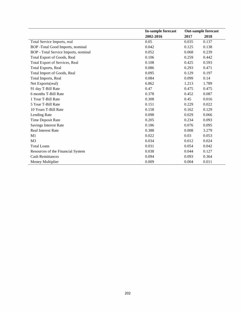
202
In-sample forecast Out-sample forecast 2002-2016 2017 2018
Total Service Imports, real 0.05 0.035 0.137
BOP -Total Good Imports, nominal 0.042 0.125 0.138
BOP - Total Service Imports, nominal 0.052 0.068 0.239
Total Export of Goods, Real 0.106 0.259 0.442
Total Export of Services, Real 0.108 0.425 0.593
Total Exports, Real 0.086 0.293 0.471
Total Import of Goods, Real 0.095 0.129 0.197
Total Imports, Real 0.084 0.099 0.14
Net Exports(real) 6.862 1.213 1.789
91 day T-Bill Rate 0.47 0.475 0.475
6 months T-Bill Rate 0.378 0.452 0.087
1 Year T-Bill Rate 0.308 0.45 0.016
5 Year T-Bill Rate 0.151 0.229 0.022
10 Years T-Bill Rate 0.158 0.162 0.129
Lending Rate 0.098 0.029 0.066
Time Deposit Rate 0.205 0.234 0.093
Savings Interest Rate 0.186 0.076 0.095
Real Interest Rate 0.388 0.008 3.279
M1 0.022 0.03 0.053
M3 0.034 0.012 0.024
Total Loans 0.031 0.054 0.042
Resources of the Financial System 0.038 0.044 0.127
Cash Remittances 0.094 0.093 0.364
Money Multiplier 0.009 0.004 0.011

203
APPENDIX 5: Documentation of creating consistent data series
1. Total and sectoral employment (tot_emp, emp_agri, emp_ind, emp_ser).
Total employment data have the following breaks:
Break 1: Past week reference period and covered household population 10 years old and over
(1956-1976 August).
Break 2: Past quarter reference period and covered household population 15 years old and over
(1976-1987 first quarter) in thousands
Break 3: Past week reference period (July 1986-2016)
Since there is an overlap in 1986 between breaks 2 and 3, a factor is computed using two
overlapping data on total employment. We use this factor to find the total employment data in
1985 that is consistent with the break 3 series. Since there is now an overlap in breaks 2 and 3 in
1985, a factor is computed again, which is used to get the data in 1984. This is done until the series
has reached 1956 (the first year of the break 1 series).
In terms of sectoral employment, there is a consistent data series from 1991 to 2016. To get
employment shares for the earlier years, Orbeta (2002) has recorded sectoral employment shares
in 1978, 1980, 1985, and 1990. A linear extrapolation has been done using this information. This
completes the series in sectoral employment shares for 1978-2016. Using this series and the total
employment generated above, sectoral employment data (level) are generated.
2. Labor Force (lf) and Unemployment Rate (unemp_rate).
Similar to the employment data, labor force data and unemployment rate data have three breaks.
To get data series earlier than 1986, a procedure similar to (1) is followed.
3. Wage index for Agriculture (wageind_agri).
These data are derived from the Nominal Agricultural Wage Rates of Farm Workers by Type of
Farm Workers published by the PSA. These are divided by the CPI and indexed to 1978 prices to
be consistent with the wage index for other sectors, all of which are publicly available.
4. Compensation of Employees, From the Rest of the World (ROW), net and Property
Income, Net
The official data for these variables originally contained 4 breaks (1946-1994, 1980-1998, 1995-
2009 and 2009-present). Right Side Scaling adjustment using raising factor was utilized in order
to harmonize the series.

204
5. Components of Gross Domestic Capital Formation (Fixed Capital + Change in Inventories)
(gdcf_fc_n and gdcf_ci_n)
These components have two data series due to changes in base years. One series (from 1946 to
2000) at 1985 prices and another series (from 1998 to 2016) at 2000 prices. In order to create a
single time-series, the shares of these components are computed using the Total GDCF, which are
also available in 2 series. The computed shares are then multiplied by the Total GDCF (at 2000
prices), which are available from 1946-2016, to create a series of Fixed Capital and Change in
Inventories at 2000 prices from 1946-1997.
6. Components Gross Domestic Capital Formation: Construction, Intellectual Property
Product, Durable Equipment, Breeding Stock and Orchard Development (gdcf_fc_cons_n,
gdcf_fc_ipp_n, gdcf_fc_dur_n, gdcf_ci_n , and gdcf_fc_breed_n)
Similar to (5), these components have two data series due to rebasing. A similar procedure done
in (5) is also done to create data series at 2000 prices. The computed shares are then multiplied by
the Fixed Capital generated in (5) to get the data on Construction, Intellectual Property Product,
Durable Equipment, Breeding Stock and Orchard Development.
7. Gross Domestic Capital Formation components: Public Construction, Private
Construction, (gdcf_fc_pubcons_n, gdcf_fc_privcons_n)
Similar to (5), these components have two data series due to rebasing. A similar procedure done
in (5) is also done to create data series at 2000 prices. The computed shares are then multiplied by
the Total Construction (at 2000 prices) to get the data series for Public Construction and Private
Construction at 2000 prices.
8. Goods export categories include electric components exports, agricultural exports,
mineral components exports, and other manufactured goods exports. Electric components
are being modelled as this is a growing export product for the Philippines in recent years.
Agricultural exports are a staple as well as with mineral components exports. Other
manufactured goods are lumped together.
Services export categories include computer services exports (business process
outsourcing), tourism exports, and other services exports. Considering that the Philippines
has a growing BPO industry, singling out these services is important for policy analysis.
Tourism exports are also a growing sector in the Philippines. Other services exports are
lumped together.
Goods import categories include machinery and equipment imports, material inputs
imports, fuel imports, rice/agricultural imports, and other imports. Machinery and
equipment together with material inputs are important goods for the growth of industry
which is why these have been singled out as individual categories. Fuel imports are
likewise a staple. With the increased importation of rice, agricultural imports have been
singled out as well. Other imports are lumped together.

205
Services imports are lumped only as total services imports. No breakdown has been made
for this.
9. Regrouping of PSA National Income Accounts’ Goods Exports Categories
Table 1 PSA National Income Accounts (1967-1991), Goods Exports
Regrouped Goods Export Categories
Export Categories
PSA National Income Accounts (1967-1991) Electronics Agricultural Mineral
Other
Manufactured
Goods
1. Semiconductors and electronic microcircuits
2. Garments
3. Crude coconut oil
4. Bars, rods of copper
5. Gold from copper ores
6. Banana and plantains
7. Lumbers
8. Copper concentrates
9. Shrimp and prawns
10. Canned pineapple
11. Iron agglomerates
12. Centrifugal sugar
13. Copra oil, cake & meal
14. Coffee, not roasted
15. Plywood, ordinary
16. Prepared tuna
17. Desiccated coconut
18. Logs
19. Others
20. Monetization of gold
Table 2 PSA National Income Accounts (1991-2000), Goods Exports
Regrouped Goods Export Categories
Export Categories
PSA National Income Accounts (1991-2000) Electronics Agricultural Mineral
Other
Manufactured
Goods
1. Garments
2. Semiconductors and electric microcircuits
3. Finished electrical machinery
4. Other products manufactured
5. Ignition wiring sets
6. Crude coconut oil
7. Bars, rods of copper
8. Shrimps and prawns
9. Gold from copper ores
10. Banana and plantains
11. Transmission apparatus
12. Copper concentrates
13. Canned pineapple
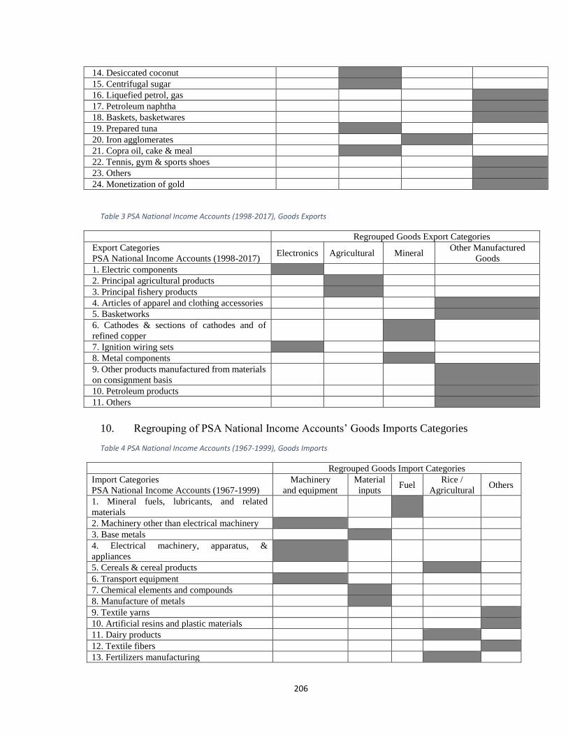
206
14. Desiccated coconut
15. Centrifugal sugar
16. Liquefied petrol, gas
17. Petroleum naphtha
18. Baskets, basketwares
19. Prepared tuna
20. Iron agglomerates
21. Copra oil, cake & meal
22. Tennis, gym & sports shoes
23. Others
24. Monetization of gold
Table 3 PSA National Income Accounts (1998-2017), Goods Exports
Regrouped Goods Export Categories
Export Categories
PSA National Income Accounts (1998-2017) Electronics Agricultural Mineral
Other Manufactured
Goods
1. Electric components
2. Principal agricultural products
3. Principal fishery products
4. Articles of apparel and clothing accessories
5. Basketworks
6. Cathodes & sections of cathodes and of
refined copper
7. Ignition wiring sets
8. Metal components
9. Other products manufactured from materials
on consignment basis
10. Petroleum products
11. Others
10. Regrouping of PSA National Income Accounts’ Goods Imports Categories
Table 4 PSA National Income Accounts (1967-1999), Goods Imports
Regrouped Goods Import Categories
Import Categories
PSA National Income Accounts (1967-1999)
Machinery
and equipment
Material
inputs Fuel
Rice /
Agricultural Others
1. Mineral fuels, lubricants, and related
materials
2. Machinery other than electrical machinery
3. Base metals
4. Electrical machinery, apparatus, &
appliances
5. Cereals & cereal products
6. Transport equipment
7. Chemical elements and compounds
8. Manufacture of metals
9. Textile yarns
10. Artificial resins and plastic materials
11. Dairy products
12. Textile fibers
13. Fertilizers manufacturing
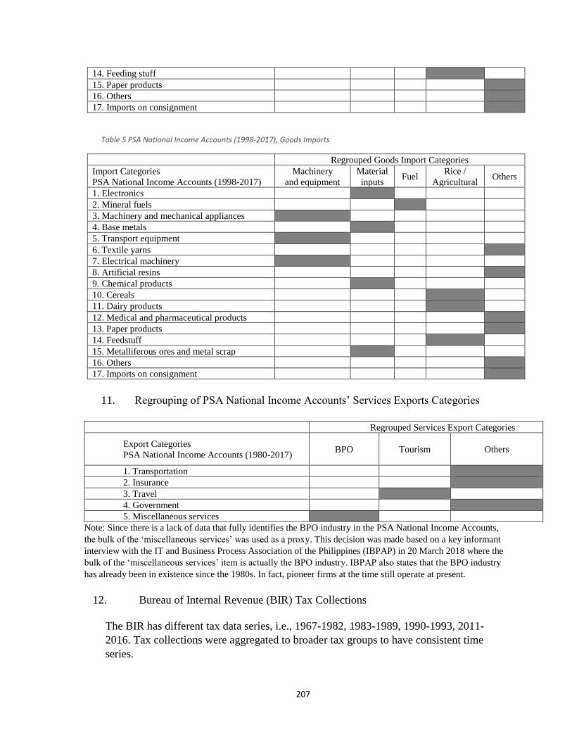
207
14. Feeding stuff
15. Paper products
16. Others
17. Imports on consignment
Table 5 PSA National Income Accounts (1998-2017), Goods Imports
Regrouped Goods Import Categories
Import Categories
PSA National Income Accounts (1998-2017)
Machinery
and equipment
Material
inputs Fuel
Rice /
Agricultural Others
1. Electronics
2. Mineral fuels
3. Machinery and mechanical appliances
4. Base metals
5. Transport equipment
6. Textile yarns
7. Electrical machinery
8. Artificial resins
9. Chemical products
10. Cereals
11. Dairy products
12. Medical and pharmaceutical products
13. Paper products
14. Feedstuff
15. Metalliferous ores and metal scrap
16. Others
17. Imports on consignment
11. Regrouping of PSA National Income Accounts’ Services Exports Categories
Regrouped Services Export Categories
Export Categories
PSA National Income Accounts (1980-2017) BPO Tourism Others
1. Transportation
2. Insurance
3. Travel
4. Government
5. Miscellaneous services
Note: Since there is a lack of data that fully identifies the BPO industry in the PSA National Income Accounts,
the bulk of the ‘miscellaneous services’ was used as a proxy. This decision was made based on a key informant
interview with the IT and Business Process Association of the Philippines (IBPAP) in 20 March 2018 where the
bulk of the ‘miscellaneous services’ item is actually the BPO industry. IBPAP also states that the BPO industry
has already been in existence since the 1980s. In fact, pioneer firms at the time still operate at present.
12. Bureau of Internal Revenue (BIR) Tax Collections
The BIR has different tax data series, i.e., 1967-1982, 1983-1989, 1990-1993, 2011-
2016. Tax collections were aggregated to broader tax groups to have consistent time
series.
208
13. Effective tax rates
Commodity-specific effective tax rates were calculated using the official tax schedules
weighted by actual or proxy measures for each commodity-schedule pair. For example,
for the effective individual income tax rate, tax schedules from the different Internal
Revenue Codes were applied to the distribution of per capita income from the Family
Income and Expenditure Surveys.
14. Household Final Consumption Expenditure (HFCE)
Older National Accounts HFCE series from NSCB and PSA were harmonized to newer
series by using the ratio of the value of the older series to the newer series at series breaks.
Some consumption items were aggregated for consistency across time. Others that require
more detailed breakdown, e.g. tobacco and alcoholic beverages, were disaggregated from
a more aggregated series using ratios derived from the triennial Family Income and
Expenditure Surveys.
15. General Government Income and Outlay Account
The General Government Income and Outlay Account estimates from NSCB and PSA
were harmonized using a similar technique employed for HFCE. Older National Accounts
HFCE series from NSCB and PSA were harmonized to newer series by using the ratio of
the value of the older series to the newer series at series breaks.