introductory dynamic macroeconomics - folk.uio.nofolk.uio.no/rnymoen/econ3410_h09_idm_aug18.pdf ·...
TRANSCRIPT
Introductory DynamicMacroeconomics
Ragnar NymoenUniversity of Oslo
18 August 2009

ii
Contents
Preface v
1 Dynamic models in economics 11.1 Introduction . . . . . . . . . . . . . . . . . . . . . . . . . . . . . . . . 11.2 Statics and dynamics in economic analysis . . . . . . . . . . . . . . . 31.3 When is a dynamic approach “required”? . . . . . . . . . . . . . . . 131.4 The distinction between a short-run model and a long-run model . . 141.5 Some milestones in the development of dynamic macroeconomics . . 181.6 Stock and flow variables . . . . . . . . . . . . . . . . . . . . . . . . . 191.7 Summary and overview of the rest of the book . . . . . . . . . . . . 23
2 Linear dynamic models 252.1 The autoregressive distributed lag model and dynamic multipliers . 25
2.1.1 The effects of a temporary change: dynamic multipliers . . . 262.1.2 The effects of a permanent change: cumulated interim multi-
pliers . . . . . . . . . . . . . . . . . . . . . . . . . . . . . . . 272.2 An example: dynamic effects of increased income on consumption . . 302.3 A typology of single equation linear models . . . . . . . . . . . . . . 342.4 More examples of dynamic relationships in economics . . . . . . . . 38
2.4.1 The dynamic consumption function (revisited) . . . . . . . . 382.4.2 The price Phillips curve . . . . . . . . . . . . . . . . . . . . . 382.4.3 Exchange rate dynamics . . . . . . . . . . . . . . . . . . . . . 40
2.5 Error correction . . . . . . . . . . . . . . . . . . . . . . . . . . . . . . 422.6 The two interpretations of static equations . . . . . . . . . . . . . . . 462.7 Solution and simulation of dynamic models . . . . . . . . . . . . . . 49
2.7.1 The solution of ADL equations . . . . . . . . . . . . . . . . . 492.7.2 Simulation of dynamic models . . . . . . . . . . . . . . . . . 55
2.8 Dynamic systems . . . . . . . . . . . . . . . . . . . . . . . . . . . . . 572.8.1 A dynamic income-expenditure model . . . . . . . . . . . . . 572.8.2 The method with a short-run and long-run model . . . . . . 582.8.3 The basic Solow growth model . . . . . . . . . . . . . . . . . 592.8.4 A real business cycle model . . . . . . . . . . . . . . . . . . . 642.8.5 The solution of the bivariate first order system (VAR) . . . . 69
iii
iv CONTENTS
3 Wage-price dynamics 733.1 Introduction . . . . . . . . . . . . . . . . . . . . . . . . . . . . . . . . 733.2 Wage bargaining and incomplete competition. . . . . . . . . . . . . . 75
3.2.1 A bargaining theory of the steady state wage . . . . . . . . . 753.2.2 Wage bargaining and dynamics . . . . . . . . . . . . . . . . . 793.2.3 Wage bargaining and inflation . . . . . . . . . . . . . . . . . . 823.2.4 The Norwegian model of inflation . . . . . . . . . . . . . . . . 843.2.5 A simulation model of wage dynamics . . . . . . . . . . . . . 893.2.6 The main-course model and the Scandinavian model of inflation 933.2.7 Wage-price curves and the NAIRU/natural rate of unemploy-
ment . . . . . . . . . . . . . . . . . . . . . . . . . . . . . . . 933.2.8 Role of exchange rate regime . . . . . . . . . . . . . . . . . . 97
3.3 The open economy Phillips curve . . . . . . . . . . . . . . . . . . . . 983.4 Summing up the Norwegain model of inflation and the Phillips curve
model . . . . . . . . . . . . . . . . . . . . . . . . . . . . . . . . . . . 1053.5 Norwegian evidence . . . . . . . . . . . . . . . . . . . . . . . . . . . . 107
3.5.1 A Phillips curve model . . . . . . . . . . . . . . . . . . . . . . 1073.5.2 An error correction wage model . . . . . . . . . . . . . . . . . 111
3.6 The New Keynesian Phillips curve . . . . . . . . . . . . . . . . . . . 1133.6.1 The ‘pure’ NPC model . . . . . . . . . . . . . . . . . . . . . . 1133.6.2 A NPC system . . . . . . . . . . . . . . . . . . . . . . . . . . 1163.6.3 The hybrid NPC model . . . . . . . . . . . . . . . . . . . . . 1183.6.4 The empirical status of the NPC model . . . . . . . . . . . . 118
A Variables and relationships in logs 125
B Linearization of the Solow model 131
Preface
These notes are written for the course ECON 3410 /4410 Introductory DynamicMacroeconomics at the University of Oslo. They contain a presentation of the keyconcepts and models required for starting to address positive macrodynamics in asystematic way, for example in connection with the master thesis in economics. Thelevel of mathematics used does not go beyond basic calculus and simple algebra.
Several students and colleagues have already contributed to this project by of-fering their comments and corrections, in particular Roger Hammersland, ThomasLystad, Andreas Ringen, and Eivind Tveter.
c° Ragnar Nymoen 2009.
v

vi PREFACE
Chapter 1
Dynamic models in economics
In this chapter we introduce the distinction between static and dy-namic models in economics. The concepts are explained with the aidof the standard model of supply and demand in a single market. Staticmodels are of most relevance when the speed of adjustment is so fastthat market disequilibria are corrected with only negligible time lags.Dynamic models become necessary when adjustment lags cannot be ig-nored without significant loss of relevance for the economic phenomenathat we want to understand and analyze. Despite these differences, sta-tic and dynamic models are related in two important respects: First,a static relationship can be seen as a limiting case of a dynamic rela-tionship. Second, static equations can be used to analyze the stationarystate of a dynamic system. Dynamic analysis is simplified by formulat-ing separate models for the short-run and for the long-run equilibrium,and this methodology is also introduced in this chapter. Another impor-tant conceptual distinction, namely between stock and flow variables, isexplained at the end of the chapter.
1.1 Introduction
In many areas of economics time plays an important role: firms and households donot react instantly to changes in for example taxes, wages and business prospects.One source of adjustment lags are found in information lags: It usually takes timebefore changes in economic circumstances are recognized or reported statistically,so that adaptive action is taken by households, firms and the government. Anothersource of time lags is that fast and full adjustment may be more costly, or inducelarger risk, than moderate and partial adjustment.
Economic activity is influenced by social norms, and markets function withina framework defined by institutions and by legislation. Often, these wider institu-tional aspects help explain why gradual adjustment is typical of economic behav-iour. Annual collective wage bargaining is an example of such an institution, which
1
2 CHAPTER 1. DYNAMIC MODELS IN ECONOMICS
helps explain the relatively smooth development of the average wage level in manyeconomies. The manufacturing of goods is not instantaneous but takes consider-able time, even years in the case of projects with huge capital investment. Finally,dynamic behaviour is also induced by the fact that many economic decisions areinfluenced by what firms, households and the government believe about the future.Often expectation formation will attribute a large weight to past developments, sincerational anticipations usually build on experience.
Economic dynamics often take the form of delayed reactions to changes in eco-nomic incentives, this delay is not the defining characteristic of dynamics. Instan-taneous changes, which takes place in the same time period as the shock occurs, isoften part of a dynamic process.. A classic example, which we shall study in somedetail in the next section, is the case of a single market characterized by perfectcompetition. A demand shift in such a market will lead to an immediate change inthe (market clearing) price.
The hallmark of dynamic adjustments therefore, is not that the response to ashock is necessarily delayed, but that the adjustment process takes several timeperiods. The effects of shock literary ‘spill over’ to the following periods. Usingthe terminology of Ragnar Frisch, who formalized macrodynamics as a discipline,we can speak of impulses to the macroeconomic system which are propagated bythe system’s own mechanism into effects that lasts for several periods after theoccurrence of the shock.1
Because dynamic behaviour is an important feature of the real world macroecon-omy, serious policy analysis requires a dynamic approach. Hence, those responsiblefor fiscal and monetary policy use dynamic models as an aid in their decision process.In recent years, monetary policy has come to play an important role in activity reg-ulation, and the central banks in many countries have defined the rate of inflation asthe target variable of economic policy. The instrument of monetary policy nowadaysis the central bank sight deposit rate, i.e., the interest rate on banks’ deposits in thecentral bank. It is interesting to note that no central bank believe in an immediateand strong effect on the rate of inflation after a change in their interest rate. Rather,because of the many dynamic effects triggered by a change in the interest rate, cen-tral banks prepare themselves to wait a substantial amount of time before the effectof the interest rate has a noticeable impact on inflation. The following statementfrom Norges Bank [The Norwegian Central Bank] represent a typical central bankview:
Monetary policy influences the economy with long and variable lags.Norges Bank sets the interest rate with a view to stabilizing inflation atthe target within a reasonable time horizon, normally 1-3 years.2
1One of Frisch’s many influential publications is called Propagation Problems and Impulse Prob-lems in Dynamic Economics, Frisch (1933).
2See Norges Bank’s web page on monetary policy: http://www.norges-bank.no/english/monetary_policy/in_norway.html.Similar formulations can be found on the web pages of the central banks in e.g., Autralia, New-
1.2. STATICS AND DYNAMICS IN ECONOMIC ANALYSIS 3
We continue this chapter by giving the classic definition of static and dynamicmodels, which is due to Ragnar Frisch (1929,1992).3 In section 1.2 we apply Frisch’sconcepts to an equilibrium model of a single product market. Section 1.3 and 1.4discuss the choice between a static and dynamic approach in macroeconomics andwe introduce the central distinction between a model for the short-run and modelfor the long-run. Section 1.5 mentions some of the milestones in the development ofmacrodynamics, and where they appear in this text. Finally, section 1.6 introducesanother conceptual distinction, namely between stock and flow variables, which playsan important role in macrodynamics, while section 1.7 gives a summary of mainpoints and sketches the road ahead.
1.2 Statics and dynamics in economic analysis
The above examples already rationalize that dynamic behaviour by economic agents,and dynamic responses in economic systems, are typical features that we want tobe able to model. As a first step we need to establish definitions of both static anddynamic models.
At a general level, static models are used to describe, or to predict, relationshipbetween state variables, while dynamic models are used to describe, or predict, therelationships between variables which are in motion. Hence, in the terminologyinvented by Ragnar Frisch, we may talk about state laws (or static law) and laws ofmotion (dynamic laws) as synonyms for static and dynamic relationships.
Frisch also formulated a simple and operational definition of dynamics. A dy-namic theory, or model, is made up of relationships between variables that refer todifferent time periods. Conversely, when all the variables included in the theory referto the same time period (or, more generally, the model is conceptualized withouttime as an entity), the system of relationships is static.4 Hence, a genuinely dynamicmodel is not obtained by simply adding subscripts for time period to the variablesof an essentially timeless relationship. The defining characteristic of dynamic theoryis that one and the same equation (often as part of a system of equations) containsentities that refer to different time periods.
Following convention, we will use the subscript t as an index for time period. Toprovide a simple example of the differences between static and dynamic relationshipswe consider a partial equilibrium model. Let Pt denote the price prevailing in a singlemarket in time period t, and let Xt denote the demand of a good in period t. A
Zealand, The United Kingdom and Sweden.The quotation stems from the summer of 2004 (and has been unchanged since then). Before that
the corresponding passage read:“A substantial share of the effects on inflation of an interest rate change will occur within two
years. Two years is therefore a reasonable time horizon for achieving the inflation target of 2 12per
cent”.3Frisch (1992) is an English translation of (parts of) Frisch (1929). An edited version of Frisch
(1929) is available in Norwegian in Frisch (1995, Ch 11).4This definition is adopted directly from Frisch (1947, p. 71).
4 CHAPTER 1. DYNAMIC MODELS IN ECONOMICS
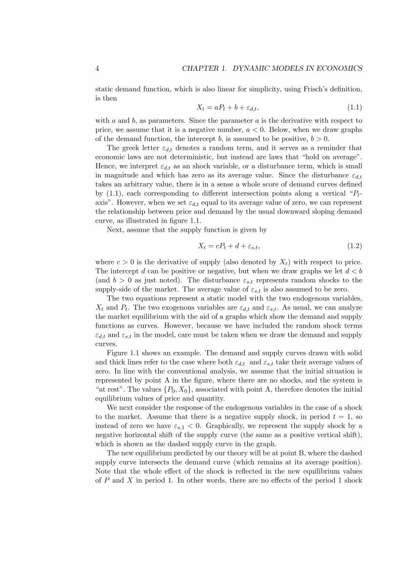
static demand function, which is also linear for simplicity, using Frisch’s definition,is then
Xt = aPt + b+ εd,t, (1.1)
with a and b, as parameters. Since the parameter a is the derivative with respect toprice, we assume that it is a negative number, a < 0. Below, when we draw graphsof the demand function, the intercept b, is assumed to be positive, b > 0.
The greek letter εd,t denotes a random term, and it serves as a reminder thateconomic laws are not deterministic, but instead are laws that “hold on average”.Hence, we interpret εd,t as an shock variable, or a disturbance term, which is smallin magnitude and which has zero as its average value. Since the disturbance εd,ttakes an arbitrary value, there is in a sense a whole score of demand curves definedby (1.1), each corresponding to different intersection points along a vertical “Pt-axis”. However, when we set εd,t equal to its average value of zero, we can representthe relationship between price and demand by the usual downward sloping demandcurve, as illustrated in figure 1.1.
Next, assume that the supply function is given by
Xt = cPt + d+ εs,t, (1.2)
where c > 0 is the derivative of supply (also denoted by Xt) with respect to price.The intercept d can be positive or negative, but when we draw graphs we let d < b(and b > 0 as just noted). The disturbance εs,t represents random shocks to thesupply-side of the market. The average value of εs,t is also assumed to be zero.
The two equations represent a static model with the two endogenous variables,Xt and Pt. The two exogenous variables are εd,t and εs,t. As usual, we can analyzethe market equilibrium with the aid of a graphs which show the demand and supplyfunctions as curves. However, because we have included the random shock termsεd,t and εs,t in the model, care must be taken when we draw the demand and supplycurves.
Figure 1.1 shows an example. The demand and supply curves drawn with solidand thick lines refer to the case where both εd,t and εs,t take their average values ofzero. In line with the conventional analysis, we assume that the initial situation isrepresented by point A in the figure, where there are no shocks, and the system is“at rest”. The values {P0,X0}, associated with point A, therefore denotes the initialequilibrium values of price and quantity.
We next consider the response of the endogenous variables in the case of a shockto the market. Assume that there is a negative supply shock, in period t = 1, soinstead of zero we have εs,1 < 0. Graphically, we represent the supply shock by anegative horizontal shift of the supply curve (the same as a positive vertical shift),which is shown as the dashed supply curve in the graph.
The new equilibrium predicted by our theory will be at point B, where the dashedsupply curve intersects the demand curve (which remains at its average position).Note that the whole effect of the shock is reflected in the new equilibrium valuesof P and X in period 1. In other words, there are no effects of the period 1 shock
1.2. STATICS AND DYNAMICS IN ECONOMIC ANALYSIS 5
Supply curve (average position)Demand curve(average position)
Pt
Xt
A
B
X0
P0
C
P1
X1
D
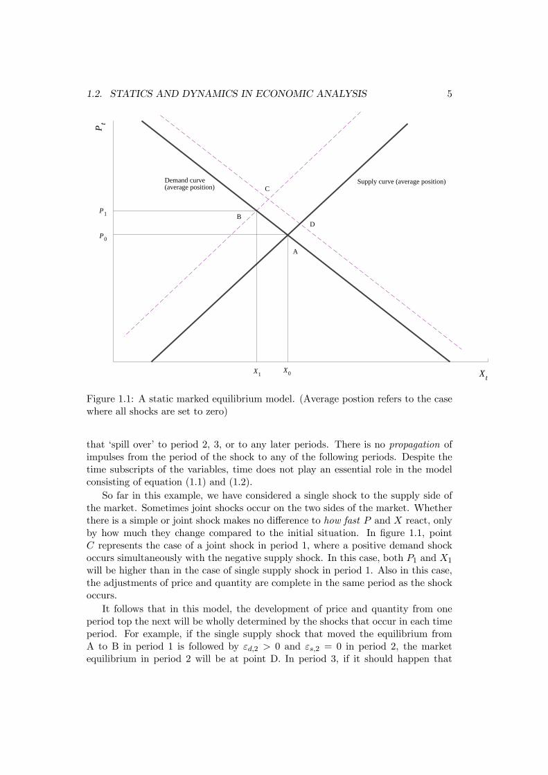
Figure 1.1: A static marked equilibrium model. (Average postion refers to the casewhere all shocks are set to zero)
that ‘spill over’ to period 2, 3, or to any later periods. There is no propagation ofimpulses from the period of the shock to any of the following periods. Despite thetime subscripts of the variables, time does not play an essential role in the modelconsisting of equation (1.1) and (1.2).
So far in this example, we have considered a single shock to the supply side ofthe market. Sometimes joint shocks occur on the two sides of the market. Whetherthere is a simple or joint shock makes no difference to how fast P and X react, onlyby how much they change compared to the initial situation. In figure 1.1, pointC represents the case of a joint shock in period 1, where a positive demand shockoccurs simultaneously with the negative supply shock. In this case, both P1 and X1
will be higher than in the case of single supply shock in period 1. Also in this case,the adjustments of price and quantity are complete in the same period as the shockoccurs.
It follows that in this model, the development of price and quantity from oneperiod top the next will be wholly determined by the shocks that occur in each timeperiod. For example, if the single supply shock that moved the equilibrium fromA to B in period 1 is followed by εd,2 > 0 and εs,2 = 0 in period 2, the marketequilibrium in period 2 will be at point D. In period 3, if it should happen that
6 CHAPTER 1. DYNAMIC MODELS IN ECONOMICS
10 20 30 40 50
−0.01
0.00
0.01
0.02
0.03
Static marked equilibrium model
market price net demand shock
0 5 10 15 20
0.25
0.50
0.75
1.00Static marked equilibrium model
Dynamic multipliers
0 5 10 15 20
−0.5
0.0
0.5
1.0 Dynamic marked equilibrium model
Dynamic multipliers
10 20 30 40 50
−0.025
0.000
0.025
0.050
Dynamic marked equilibrium model
market price net demand shock
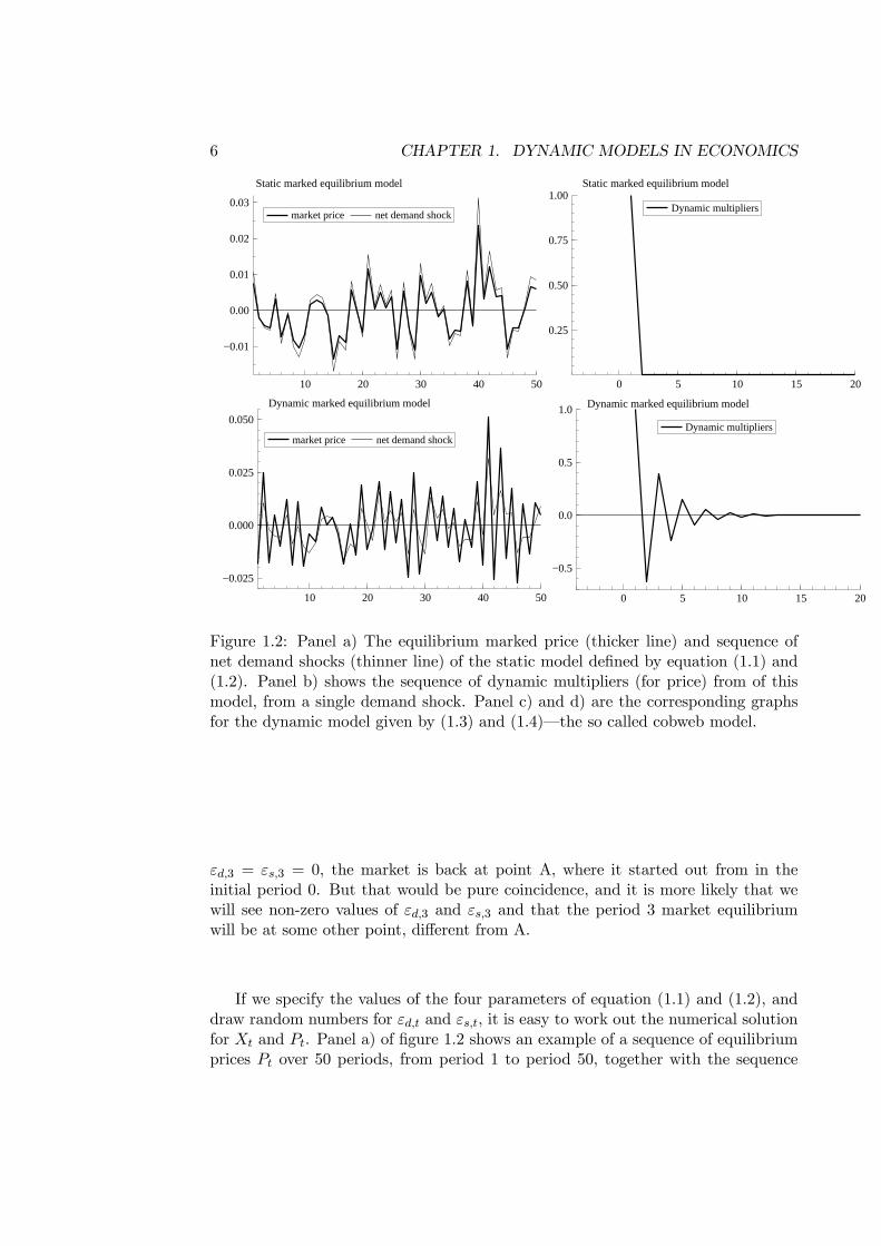
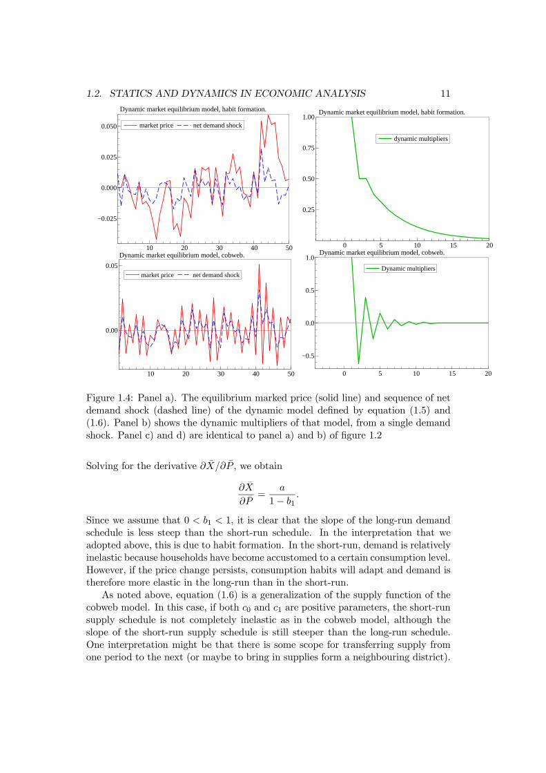
Figure 1.2: Panel a) The equilibrium marked price (thicker line) and sequence ofnet demand shocks (thinner line) of the static model defined by equation (1.1) and(1.2). Panel b) shows the sequence of dynamic multipliers (for price) from of thismodel, from a single demand shock. Panel c) and d) are the corresponding graphsfor the dynamic model given by (1.3) and (1.4)–the so called cobweb model.
εd,3 = εs,3 = 0, the market is back at point A, where it started out from in theinitial period 0. But that would be pure coincidence, and it is more likely that wewill see non-zero values of εd,3 and εs,3 and that the period 3 market equilibriumwill be at some other point, different from A.
If we specify the values of the four parameters of equation (1.1) and (1.2), anddraw random numbers for εd,t and εs,t, it is easy to work out the numerical solutionfor Xt and Pt. Panel a) of figure 1.2 shows an example of a sequence of equilibriumprices Pt over 50 periods, from period 1 to period 50, together with the sequence
1.2. STATICS AND DYNAMICS IN ECONOMIC ANALYSIS 7
of random shocks that drives the solution.5 There are random supply and demandshocks in each period, so in the graph we have chosen to show the net demandshocks: εd,t − εs,t.
Note how closely the graph of the equilibrium price follows the graph of randomshocks. As we have seen, this is because of the static nature of the model, whichimplies that the price in any period, for example period 20, reflects the random“excess demand” of that period. No other stochastic shocks, before or after, influencethe equilibrium price P20 for example.
The underlying model characteristic is therefore that the endogenous variablesof the static mode adjust fully to a shock to the system, within the same periodof the shock. There are no spill-over effects of a shock to the following period, orto subsequent periods. The graph in panel b) of figure 1.2 is an example of a socalled dynamic multiplier. It shows how the response of an endogenous variable (themarket price in this case) develops over time. In this case, the graph of the dynamicmultiplier simply reflects that it is derived from a static model: the whole responsetakes place within the period of the shock, and all the responses are zero in all theperiods after the shock. Dynamic models, where time plays an essential role, willgenerate dynamic multipliers which have a much more interesting shape. So let usconsider genuine dynamics!
As a first example of a dynamic model, we keep the demand equation (1.1):
Xt = aPt + b+ εd,t, (1.3)
but the supply function (1.2) is replaced by
Xt = cPt−1 + d+ εs,t (1.4)
with parameter c > 0. In terms of economic interpretation, equation (1.4) mayrepresent a case of important production and delivery lags, so that today’s supplydepends of the price obtained in the previous period. The classic example is fromagricultural economics, where the whole supply, for example of pork or of wheat,is replenished from one year to the next.6 Another interpretation, see Evans andHonkapoja (2001), which captures that the underlying behaviour of suppliers maybe influenced by expectations, starts from
Xt = cP et + d+ εs,t
where P et denotes the expected price in period t, as in the so-called Lucas supply
function, see Lucas (1976). If we assume that information about period t is either5 In this book we often use figures with multiple graphs, such as Figure 1.2. In the text, we refer
to the panels as a), b) etc, according to the rule
a bc d
for a 2× 2 figure. In the case of a 3× 3 figure for example, c) denotes the third panel of the firstrow, while e) is the third panel of the second row.
6Named by Niclas Kaldor, cf. Kaldor (1934).
8 CHAPTER 1. DYNAMIC MODELS IN ECONOMICS
unavailable, or is very unreliable in period t − 1, when expectations are formed,suppliers have to set P e
t = Pt−1, and we retrieve the dynamic supply function (1.4).Clearly, using Frisch’s definition, equation (1.4) qualifies as a dynamic model of
the supplied quantity since “one and the same equation contains entities that referto different time periods”, namely Xt and Pt−1. What about the model as a whole,i.e., the system given by the static equation (1.3) and the dynamic equation (1.4)?Is this a static or dynamic system? To answer this question we consider figure 1.3.
In figure 1.3, the line of the demand curve has the same interpretation as in thestatic model in figure 1.1. However, care must taken when interpreting the supplycurve. To understand why, consider the quantity supplied in period t = 1, assumingthat t = 0 represents the initial situation with εs,0 = 0. According to (1.4), supplyis given by
X1 = cP0 + d,
since supply in period 1 is a function of P0 which is already determined (fromhistory), and not the price in period 1. The supply in period 1, which we can callshort-run supply, is therefore completely inelastic with respect to the price, P1.
Unlike figure 1.1, where the supply curve represents the short-run response ofsupply with respect to a price change, the positively sloped supply schedule in figure1.3 therefore refers to a different type of price variation. This variation is counter-factual and refers to a hypothetical stationary situation where, εs,t = 0 for all t, andPt = Pt−1 = P , and Xt = X. It is conventional terminology to use “stationary sit-uation” and “long-run situation” as synonyms, and accordingly the upward slopingcurve in in figure 1.3 has been dubbed the long-run supply curve. Mathematicallyit is defined by:
X = cP + d,
and c is called the long-run derivative of the supply function. It is the increase insupply that would have resulted if the price had been increased by one unit and hadstayed at that new level forever.
We next turn to the system’s response to a shock. We consider a positive (hori-zontal) demand shift, represented by the dashed demand schedule in figure 1.3. Inthe same way as in the first example, we assume that initially the system is ‘at rest’at point A, so that {P0,X0} denotes the initial situation. In period 1 the demandshock (εd,1 > 0) occurs, as indicated. Since short-run supply is completely inelastic,the market equilibrium in period 1 is at point B, with the market clearing price-quantity combination {P1,X0}. Note that X1 = X0, since the quantity supplied isalready determined by the price that prevailed in the market in the past period.
In the same way as in the analysis of the static model, we assume that thedemand shock disappears in period 2, so the demand schedule shifts back to itsaverage position. However, since the price P1 leads to increased supply in period 2,namely X2 −X1 = c(P1−P0), the period 2 equilibrium is at point C, with price P2which is lower than the initial price P0. The traded quantity X2 is also different fromthe initial value X0, reflecting that the price was high in period 1. Hence, both priceand quantity react dynamically to the demand shock in period 1. The effect of the
1.2. STATICS AND DYNAMICS IN ECONOMIC ANALYSIS 9
Long−run supply curve
Demand curve(average position)
Pt
Xt
A
B
X0
P0
C
X2
P1
P2
D
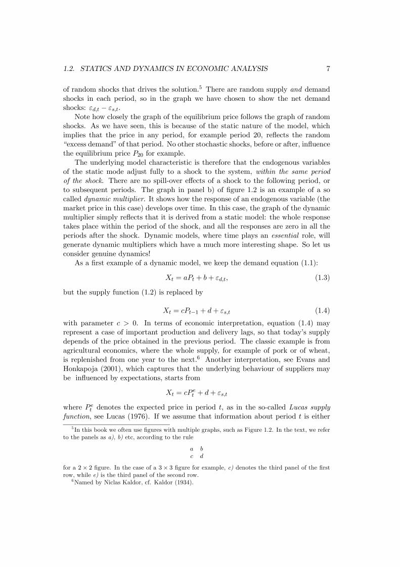
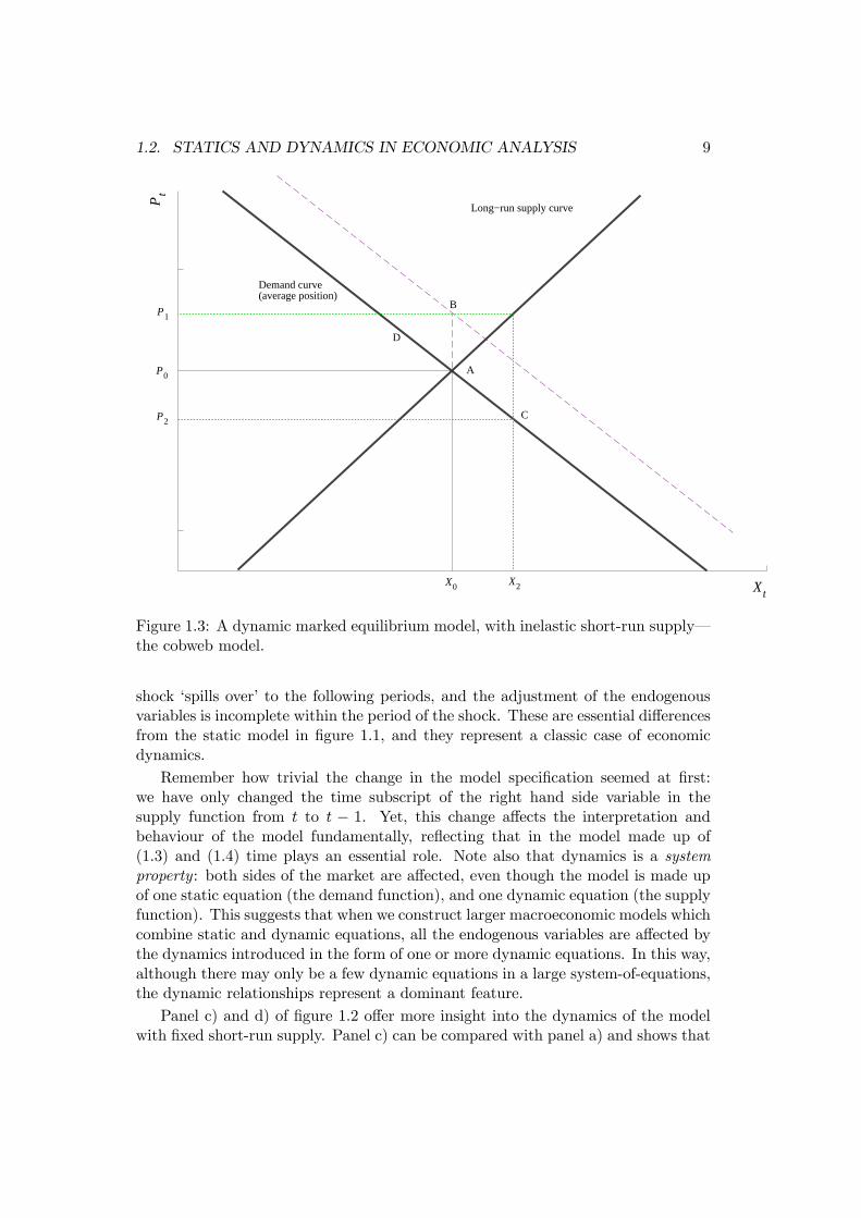
Figure 1.3: A dynamic marked equilibrium model, with inelastic short-run supply–the cobweb model.
shock ‘spills over’ to the following periods, and the adjustment of the endogenousvariables is incomplete within the period of the shock. These are essential differencesfrom the static model in figure 1.1, and they represent a classic case of economicdynamics.
Remember how trivial the change in the model specification seemed at first:we have only changed the time subscript of the right hand side variable in thesupply function from t to t − 1. Yet, this change affects the interpretation andbehaviour of the model fundamentally, reflecting that in the model made up of(1.3) and (1.4) time plays an essential role. Note also that dynamics is a systemproperty: both sides of the market are affected, even though the model is made upof one static equation (the demand function), and one dynamic equation (the supplyfunction). This suggests that when we construct larger macroeconomic models whichcombine static and dynamic equations, all the endogenous variables are affected bythe dynamics introduced in the form of one or more dynamic equations. In this way,although there may only be a few dynamic equations in a large system-of-equations,the dynamic relationships represent a dominant feature.
Panel c) and d) of figure 1.2 offer more insight into the dynamics of the modelwith fixed short-run supply. Panel c) can be compared with panel a) and shows that
10 CHAPTER 1. DYNAMIC MODELS IN ECONOMICS
because of the dynamics, the evolution of the market price Pt (the thicker line) ismore volatile than the net demand shock. Panel d) can be compared with panel b).It shows the dynamic multipliers of price with respect to a demand shock in period1. In this case the sequence of multipliers is much more interesting than in the staticmodel. In line with the graphical analysis above, the first multiplier (often calledthe impact multiplier) is positive, while the second is negative, the third is positive,and so on. The graphs show however, that the absolute values of the multipliersare reduced as we move away from period 1 (when the shock occurs), and after 10periods they become negligible. In figure 1.1 the dynamic response to the shockcan be illustrated by noting that the equilibrium in period 3 will be at point D onthe (average) demand curve, and noting that by joining up the equilibrium pointsa cobweb pattern emerges. The web starts at point B and ends at point A, afterseveral periods of adjustments. The model defined by equation (1.3) and (1.4) hassuccinctly been named the cobweb model.
The cobweb model is only one of the many possible types of dynamics that canoccur in a model of equilibrium in a single market. To take a different example,consider the following two demand and supply equations:
Xt = aPt + b1Xt−1 + b0 + εd,t, and (1.5)
Xt = c0Pt + c1Pt−1 + d+ εs,t. (1.6)
In this model, also the demand function (1.5) is a dynamic equation. The parameterb1 measures by how much an unit increase in Xt−1 affects demand in period t.This can be rationalized by habit formation for example, in which case we may set0 < b1 < 1, i.e., high demand today makes for high demand tomorrow as well, ceterisparibus. The second modification of the cobweb model is in the supply equation(1.6): If we assume that the parameter c0 is positive, we relax the assumption aboutcompletely inelastic short-run supply that characterized the cobweb model.
In the same way that we drew a distinction between the short-run and the long-run supply equation in the cobweb model, we can now define short-run and long-runversion of both schedules. The coefficient a is now interpreted as the slope coefficientof the short-run demand curve. Formally, the short-run slope coefficient is the partialderivative Xt with respect to Pt:
∂Xt/∂Pt = a
The long-run demand schedule is defined for the hypothetical stationary situationwhere Xt = Xt−1 = X, and Pt = P . The slope coefficient of the long-run demandfunction is defined by
∂X
∂P= a+ b1
∂X
∂P,
since in the long-run, all values of Xt are affected by a lasting change in the price.
1.2. STATICS AND DYNAMICS IN ECONOMIC ANALYSIS 11
0 5 10 15 20
−0.5
0.0
0.5
1.0Dynamic market equilibrium model, cobweb.
Dynamic multipliers
10 20 30 40 50
0.00
0.05
Dynamic market equilibrium model, cobweb.
market price net demand shock
10 20 30 40 50
−0.025
0.000
0.025
0.050
Dynamic market equilibrium model, habit formation.
market price net demand shock
0 5 10 15 20
0.25
0.50
0.75
1.00Dynamic market equilibrium model, habit formation.
dynamic multipliers
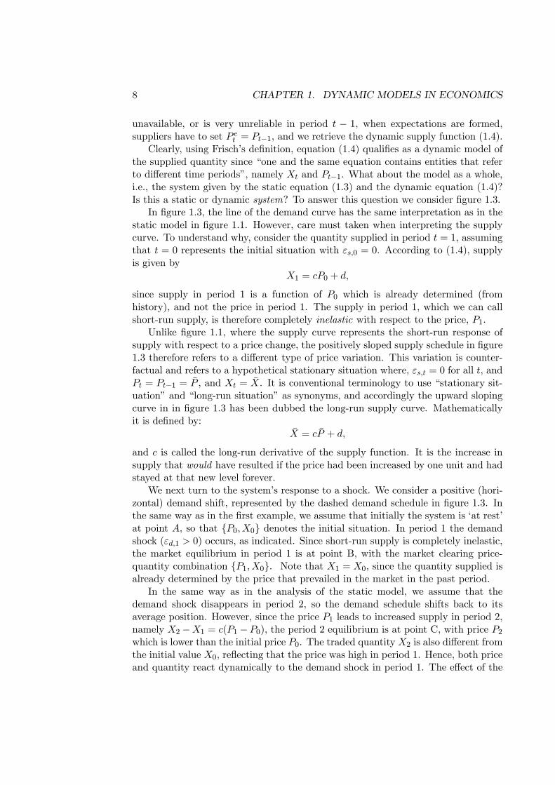
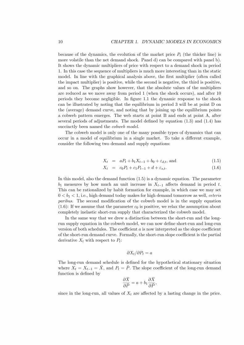
Figure 1.4: Panel a). The equilibrium marked price (solid line) and sequence of netdemand shock (dashed line) of the dynamic model defined by equation (1.5) and(1.6). Panel b) shows the dynamic multipliers of that model, from a single demandshock. Panel c) and d) are identical to panel a) and b) of figure 1.2
Solving for the derivative ∂X/∂P , we obtain
∂X
∂P=
a
1− b1.
Since we assume that 0 < b1 < 1, it is clear that the slope of the long-run demandschedule is less steep than the short-run schedule. In the interpretation that weadopted above, this is due to habit formation. In the short-run, demand is relativelyinelastic because households have become accustomed to a certain consumption level.However, if the price change persists, consumption habits will adapt and demand istherefore more elastic in the long-run than in the short-run.
As noted above, equation (1.6) is a generalization of the supply function of thecobweb model. In this case, if both c0 and c1 are positive parameters, the short-runsupply schedule is not completely inelastic as in the cobweb model, although theslope of the short-run supply schedule is still steeper than the long-run schedule.One interpretation might be that there is some scope for transferring supply fromone period to the next (or maybe to bring in supplies form a neighbouring district).
12 CHAPTER 1. DYNAMIC MODELS IN ECONOMICS
Figure 1.4, panel a) and b), illustrate the properties of model (1.5) and (1.6).Note that the market price Pt, shown as the thicker line on panel a), is more per-sistent than the net demand shock. The difference from the price behaviour of thecobweb model, which is repeated in panel c) for comparison, is striking. The in-terpretation is that in the model consisting of equation (1.5) and (1.6), a shockto demand in any given period is propagated into a demand increase (i.e. also ata given price), because of the habit formation effect. For this reason, the marketclearing price has a tendency to stay high (or low) for a longer period of time thanin the cobweb model. Propagation is in this sense stronger than in the pure cobwebmodel.
Panel d) shows how the same propagation mechanism leaves its mark on thedynamic multiplier. After a shock to demand there is a positive first multiplier, andunlike the cobweb model, the whole sequence of subsequent multipliers are positivefor this model. The equilibrium price increases after a shock, and is then reducedgradually back to the initial equilibrium level. The dynamic adjustment is thereforesmoother than in the previous model, and it is also more long-lasting. In panel b) offigure 1.4 there is still some effect left of the initial demand shock after 10 periods,while the adjustment is practically speaking complete in panel d), which is repeatedfrom the cobweb model.
Box 1.1 (Continuous and discrete time) Economic dynamicmodels are formulated in either continuous time or discrete time.Which one is used is a matter of convenience. In this book we usediscrete time to keep the theory close to real world data. Consider thecontinuous time theoretical relationship:
y = ay(t) + ε(t), a < 0, (1.7)
where y(t) and ε(t)denote variables that are continuous functions oftime, t. The left hand side variable y is the derivative of y with respectto time. a is a parameter. Time plays an essential role in model(1.7): If there is an increase in ε(t), y will be larger, and through timethere will also be an increase in y. The corresponding formulation fordiscrete time is:
yt = αyt−1 + εt, α > 0,
oryt − yt−1 = (α− 1)yt−1 + εt, α > 0, (1.8)
to make the correspondence even clearer. In (1.8),yt−yt−1 correspondsto y in (1.7), and (α− 1) corresponds to a.
1.3. WHEN IS A DYNAMIC APPROACH “REQUIRED”? 13
1.3 When is a dynamic approach “required”?
We have seen that in a static model the full effect of a shock on the endogenousvariables is reached in the same time period as the shock. In dynamic models,the endogenous variables’ responses to shocks are not instantaneous, and dynamicsystems may take several periods to adjust to a shock in period t. The exact shapesof the responses, which we dubbed dynamic multipliers above, depend on the detailsof the model specification, and on which values we give to the parameters of themodel. In the cobweb model, the multipliers were a oscillating sequence, while inthe model with habit formation, the multipliers (all positive) fell monotonically withtime. In the next chapter we will give more examples of dynamic multipliers, bothfrom theoretical models and from models that have been fitted to real world data,and we shall learn how the properties of the dynamic multipliers can be analyzedformally.
With this in mind, it lies close at hand to draw a rather far-reaching conclusion:in terms of realism, static models are only suited when the speed of adjustment ofthe variables are so fast that we can ignore that ‘actually’ there is some time delaybetween the impulse (or shock) and the response. To quote Frisch:
Hence it is clear that the static model world is best suited to the typeof phenomena whose mobility (speed of reaction) is in fact so great thatthe fact that the transition from one situation to another takes a certainamount of time can be discarded. If mobility is for some reason dimin-ished, making it necessary to take into account the speed of reaction,one has crossed into the realm of dynamic theory.7
The choice between a static and a dynamic analysis will therefore depend on what wejudge to be realistic or typical of the real world phenomenon which is the subject ofour investigation very high speed of reaction to impulses, or more moderate responsetime. Hence, somewhat paradoxically, phenomena which in an everyday meaningof the word are really dynamic, with lots of volatility, as for example stock marketprices, can be analyzed scientifically using a static framework because the speedof adjustment is so fast in the market. At least, a static model is useful firstapproximation–even though further insights almost certainly would be gained if wemanaged to formulate a dynamic model of the market. This touches upon anotherissue, namely that the choice between a static or dynamic approach is also a matterof the level of ambition for the analysis. In practice, the choice depends on how muchtime (and other resources) that we are willing to spend on our modelling exercise,and on the purpose of the analysis.
Consider for example the standard Keynesian income-expenditure model. Thisis a static model, with many omissions with regard to dynamic adjustments, butit is nevertheless widely regarded as a relevant model of short-run macroeconomic
7Frisch (1992, p 394), which is an translation of Frisch (1929). A shorthened version of Frisch’s1929 paper is accessible in Frisch (1995), the quate is from page 153.
14 CHAPTER 1. DYNAMIC MODELS IN ECONOMICS
responses to shocks. This relevance explains the strong position that the Keynesianincome-expenditure model continue to hold in macroeconomic teaching, as docu-mented in the leading textbooks, see e.g., Blanchard (2009) and Birch Sørensen andWhitta-Jacobsen (2005). There is no contradiction between this view, and at thetime also recognizing that in the longer time perspective (but still within the timehorizon of the policy analysis), the effects that increased spending have on pricesand wages for example need to be analyzed jointly with the immediate GDP effects,and that a dynamic framework is required for this purpose. One of the goals of thiscourse is to extend the standard analysis of fiscal and monetary policy analysis intothe realm of dynamic theory.
Of course, dynamic analysis is central in the theory of economics of growth, andeconomics students often first encounter dynamic models in a course in growth the-ory, specifically, the Solow model is the standard analytical framework, see Chapter2.8.3 below. This may have had the side-effect that students come to regard dy-namic models as only relevant for growth economics and other long-term issues witha time horizon of perhaps several decades. This is unfortunate, since, as we have,seen a dynamic approach may give many relevant insights also for analysis with atime horizon of (say) 1-5 years.
It is typical for the development of economics, and for its use as an aid to policyformulations, that competence in the analysis of dynamic models is in increasing de-mand by central banks, ministries of finance, international organizations and otherswhose responsibility (or business) it is to do macroeconomic analysis over a horizonof 1 to 5 years, which economists customarily refer to as the medium run.
1.4 The distinction between a short-run model and along-run model
In addition to their role as partial and approximate representations of real worldeconomic behaviour, static models play another and quite different role in macroeco-nomic analysis:Static equations express what the dynamic model would correspondto in a counterfactual situation where no shocks, impulses or changes in incentivesoccurred. As we become accustomed to dynamic analysis, we will refer to this cor-respondence by saying that static relationships can represent the stationary state(or the steady state) of a dynamic model. We will also, when no misunderstandingare likely to occur, follow custom and use the terms stationary (or steady state)equation interchangeably with the term long-run equation.
It is of some importance to understand that according to this definition, theconcept of the long-run is a relative concept. What is meant by the long-run dependson the properties of the model that we use to analyze the real-life phenomenon. Thelong-run therefore refers to the length of the adjustment period after a shock, froman initial stationary situation, to a new stationary situation is reach after all theeffects of the shock have worked their way through and “out of” the model. In thecobweb model example above, the long-run seemed to be approximately 2 years, i.e.,
1.4. THE DISTINCTION BETWEENA SHORT-RUNMODEL ANDA LONG-RUNMODEL15
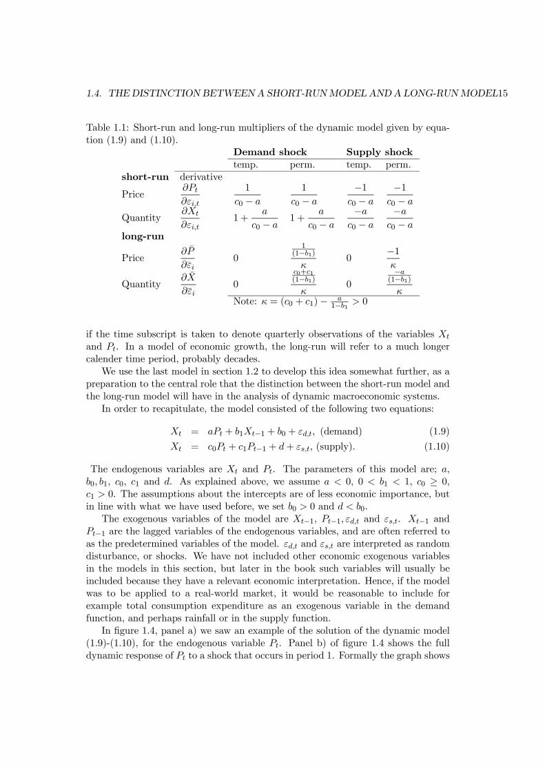
Table 1.1: Short-run and long-run multipliers of the dynamic model given by equa-tion (1.9) and (1.10).
Demand shock Supply shocktemp. perm. temp. perm.
short-run derivative
Price∂Pt∂εi,t
1
c0 − a
1
c0 − a
−1c0 − a
−1c0 − a
Quantity∂Xt
∂εi,t1 +
a
c0 − a1 +
a
c0 − a
−ac0 − a
−ac0 − a
long-run
Price∂P
∂εi0
1(1−b1)κ
0−1κ
Quantity∂X
∂εi0
c0+c1(1−b1)κ
0
−a(1−b1)κ
Note: κ = (c0 + c1)− a1−b1 > 0
if the time subscript is taken to denote quarterly observations of the variables Xt
and Pt. In a model of economic growth, the long-run will refer to a much longercalender time period, probably decades.
We use the last model in section 1.2 to develop this idea somewhat further, as apreparation to the central role that the distinction between the short-run model andthe long-run model will have in the analysis of dynamic macroeconomic systems.
In order to recapitulate, the model consisted of the following two equations:
Xt = aPt + b1Xt−1 + b0 + εd,t, (demand) (1.9)
Xt = c0Pt + c1Pt−1 + d+ εs,t, (supply). (1.10)
The endogenous variables are Xt and Pt. The parameters of this model are; a,b0, b1, c0, c1 and d. As explained above, we assume a < 0, 0 < b1 < 1, c0 ≥ 0,c1 > 0. The assumptions about the intercepts are of less economic importance, butin line with what we have used before, we set b0 > 0 and d < b0.
The exogenous variables of the model are Xt−1, Pt−1, εd,t and εs,t. Xt−1 andPt−1 are the lagged variables of the endogenous variables, and are often referred toas the predetermined variables of the model. εd,t and εs,t are interpreted as randomdisturbance, or shocks. We have not included other economic exogenous variablesin the models in this section, but later in the book such variables will usually beincluded because they have a relevant economic interpretation. Hence, if the modelwas to be applied to a real-world market, it would be reasonable to include forexample total consumption expenditure as an exogenous variable in the demandfunction, and perhaps rainfall or in the supply function.
In figure 1.4, panel a) we saw an example of the solution of the dynamic model(1.9)-(1.10), for the endogenous variable Pt. Panel b) of figure 1.4 shows the fulldynamic response of Pt to a shock that occurs in period 1. Formally the graph shows
16 CHAPTER 1. DYNAMIC MODELS IN ECONOMICS
Long−run supply curve
Long−run demand curve
P
X
Short−run demand curve
Short−run supply curve
A
BC
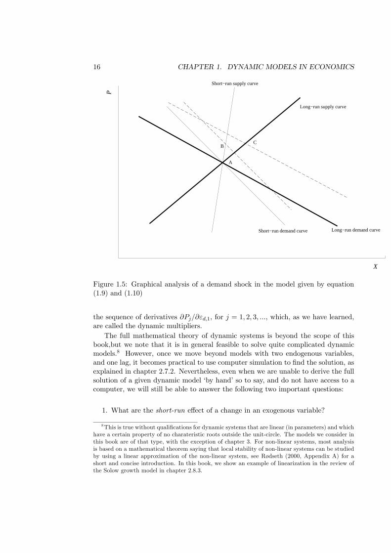
Figure 1.5: Graphical analysis of a demand shock in the model given by equation(1.9) and (1.10)
the sequence of derivatives ∂Pj/∂εd,1, for j = 1, 2, 3, ..., which, as we have learned,are called the dynamic multipliers.
The full mathematical theory of dynamic systems is beyond the scope of thisbook,but we note that it is in general feasible to solve quite complicated dynamicmodels.8 However, once we move beyond models with two endogenous variables,and one lag, it becomes practical to use computer simulation to find the solution, asexplained in chapter 2.7.2. Nevertheless, even when we are unable to derive the fullsolution of a given dynamic model ‘by hand’ so to say, and do not have access to acomputer, we will still be able to answer the following two important questions:
1. What are the short-run effect of a change in an exogenous variable?
8This is true without qualifications for dynamic systems that are linear (in parameters) and whichhave a certain property of no charateristic roots outside the unit-circle. The models we consider inthis book are of that type, with the exception of chapter 3. For non-linear systems, most analysisis based on a mathematical theorem saying that local stability of non-linear systems can be studiedby using a linear approximation of the non-linear system, see Rødseth (2000, Appendix A) for ashort and concise introduction. In this book, we show an example of linearization in the review ofthe Solow growth model in chapter 2.8.3.
1.4. THE DISTINCTION BETWEENA SHORT-RUNMODEL ANDA LONG-RUNMODEL17
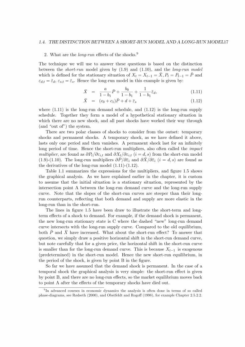
2. What are the long-run effects of the shocks.9
The technique we will use to answer these questions is based on the distinctionbetween the short-run model given by (1.9) and (1.10), and the long-run modelwhich is defined for the stationary situation of Xt = Xt−1 = X, Pt = Pt−1 = P andεd,t = εd, εs,t = εs. Hence the long-run model in this example is given by:
X =a
1− b1P +
b01− b1
+1
1− b1εd, (1.11)
X = (c0 + c1)P + d+ εs (1.12)
where (1.11) is the long-run demand schedule, and (1.12) is the long-run supplyschedule. Together they form a model of a hypothetical stationary situation inwhich there are no new shock, and all past shocks have worked their way through(and “out of”) the system.
There are two polar classes of shocks to consider from the outset: temporaryshocks and permanent shocks. A temporary shock, as we have defined it above,lasts only one period and then vanishes. A permanent shock last for an infinitelylong period of time. Hence the short-run multipliers, also often called the impactmultiplier, are found as ∂Pt/∂εi,t and ∂Xt/∂εi,t (i = d, s) from the short-run model(1.9)-(1.10). The long-run multipliers ∂P/∂εi and ∂X/∂εi (i = d, s) are found asthe derivatives of the long-run model (1.11)-(1.12).
Table 1.1 summarizes the expressions for the multipliers, and figure 1.5 showsthe graphical analysis. As we have explained earlier in the chapter, it is customto assume that the initial situation is a stationary situation, represented by theintersection point A between the long-run demand curve and the long-run supplycurve. Note that the slopes of the short-run curves are steeper than their long-run counterparts, reflecting that both demand and supply are more elastic in thelong-run than in the short-run.
The lines in figure 1.5 have been draw to illustrate the short-term and long-term effects of a shock to demand. For example, if the demand shock is permanent,the new long-run stationary state is C where the dashed “new” long-run demandcurve intersects with the long-run supply curve. Compared to the old equilibrium,both P and X have increased. What about the short-run effect? To answer thatquestion, we simply draw a positive horizontal shift in the short-run demand curve,but note carefully that for a given price, the horizontal shift in the short-run curveis smaller than for the long-run demand curve. This is because Xt−1 is exogenous(predetermined) in the short-run model. Hence the new short-run equilibrium, inthe period of the shock, is given by point B in the figure.
So far we have assumed that the demand shock is permanent. In the case of atemporal shock the graphical analysis is very simple: the short-run effect is givenby point B, and there are no long-run effects, so the market equilibrium moves backto point A after the effects of the temporary shocks have died out.
9 In advanced courses in economic dynamics the analysis is often done in terms of so calledphase-diagrams, see Rødseth (2000), and Obstfeldt and Rogoff (1998), for example Chapter 2.5.2.2.
18 CHAPTER 1. DYNAMIC MODELS IN ECONOMICS
1.5 Some milestones in the development of dynamicmacroeconomics
The motivation for the development of macrodynamics hinges on the basic rationalegiven by Frisch, namely that “in real life both inertia and friction act as a brake onspeed of reaction”.10 Frisch also noted that
The static theory’s assumption regarding an infinitely great speedof reaction contains one of the most important sources of discrepancybetween theory and experience.11
Therefore Frisch anticipated the increased use of dynamics in economics–it wouldincrease the degree of realism and scope of macroeconomic analysis. Frisch wasnot alone (for long). It seems that dynamics was “in the air” between the twoworlds wars. Frisch published his seminal article called Propagation Problems andImpulse Problems in Dynamic Economics in 1933, and the Dutch econometricianJan Tinbergen developed the first macroeconometric models of the business cycle.12
Econometricians have continued to play an important role in the development of dy-namic economics, and the field developed particularly quickly in the 1980s and 1990s.Later in the book we will introduce the concept of error correction (which we willlearn to treat synonymously with equilibrium correction) which was coined by theBritish econometrician Denis Sargan, and which is central to the modern disciplineof dynamic econometrics, as documented in Hendry (1995). From another angle, theresearch programme initiated by Finn Kydland and Edvard Prescott (1982) , andwhich utilizes relationships that have been derived from microeconomic theory tomodel representative macro agents, have become standard in macroeconomic the-ory. This research started by combining lags in the evolution of physical capital withrandom technology shocks, and the result was a dynamic macroeconomic model thatwas dubbed the real business cycle (RBC) model. A simple RBC model is presentedin chapter 2.8.4.
The RBC model can also be seen as a application of Solow’s growth modelto a shorter time period that was originally intended. Recently, there has beenfurther development in that direction in the form of micro based dynamic macromodel knows as DSGE models (Dynamic Stochastic General Equilibrium models).In chapter 3 we present one of the key elements of DSGE models, namely the modelof the supply side called the New Keynesian Phillips curve, in chapter 3.6 below.
10Frisch (1992, p 395).11Frisch (1992, p 395).12Tinbergen’s models were commissioned by the League of Nations, and they triggered the first big
metodenstreit that involved econometrics as a dicipline. Keynes was deeply critical, and Frisch hadhis own distinct views, see Frisch (1938). Trygve Haavelmo belonged to a group of econometricanswho were positive to Tinbergens pathbreaking work, cf. Haavelmo (1943). For those interested inthe formative years of dynamic economics and econometrics, the book by Morgan (1990) gives anexcellent vantage point.
1.6. STOCK AND FLOW VARIABLES 19
1.6 Stock and flow variables
In macroeconomics there is an important conceptual distinction between flow andstock variables. Examples of flow variables are GDP and its expenditure compo-nents, hours worked and inflation. Flow variables are measured in for examplemillion kroner, or thousand hours worked, per year (or quarter, or month). Infla-tion is measured as a rate, or percentage, per time period and is another exampleof a flow variable. Values of stock variables, in contrast, refer to particular pointsin time. For example, statistical numbers for national debt often refer to the end ofthe year.
Price indices are also examples of stock variables. They represent the cost ofbuying a basket of goods with reference to a particular time period. The annualconsumption price index, CPI for short, is a stock variable which is obtained as theaverage of the 12 monthly indices (each being a stock variable).
For example Pt may represent the value of the Norwegian CPI in period t (amonth, a quarter or a year). As you probably will know from before, the values of Pwill be index numbers. The number 100 (often 1 is used instead) refers to the baseperiod of the index. If Pt > 100 the overall price level is higher in period t than inthe base year–there has been a period of inflation.
Starting from a stock variable like Pt, flow variables can be obtained by calcu-lating (some sort of) difference between Pt and Pt−1. For example
xt = Pt − Pt−1, the (absolute) change
yt =Pt − Pt−1
Pt−1, the relative change, and
zt = lnPt − lnPt−1 the approximate relative change
are all flow variables derived from the stock variable Pt. Note that:
• yt× 100 is inflation in percentage points. In this book we will often use to therate formulation , hence we omit the scaling by 100.
• zt ≈ yt by the properties of the (natural) logarithmic function, see for examplethe appendix A if you are in doubt.
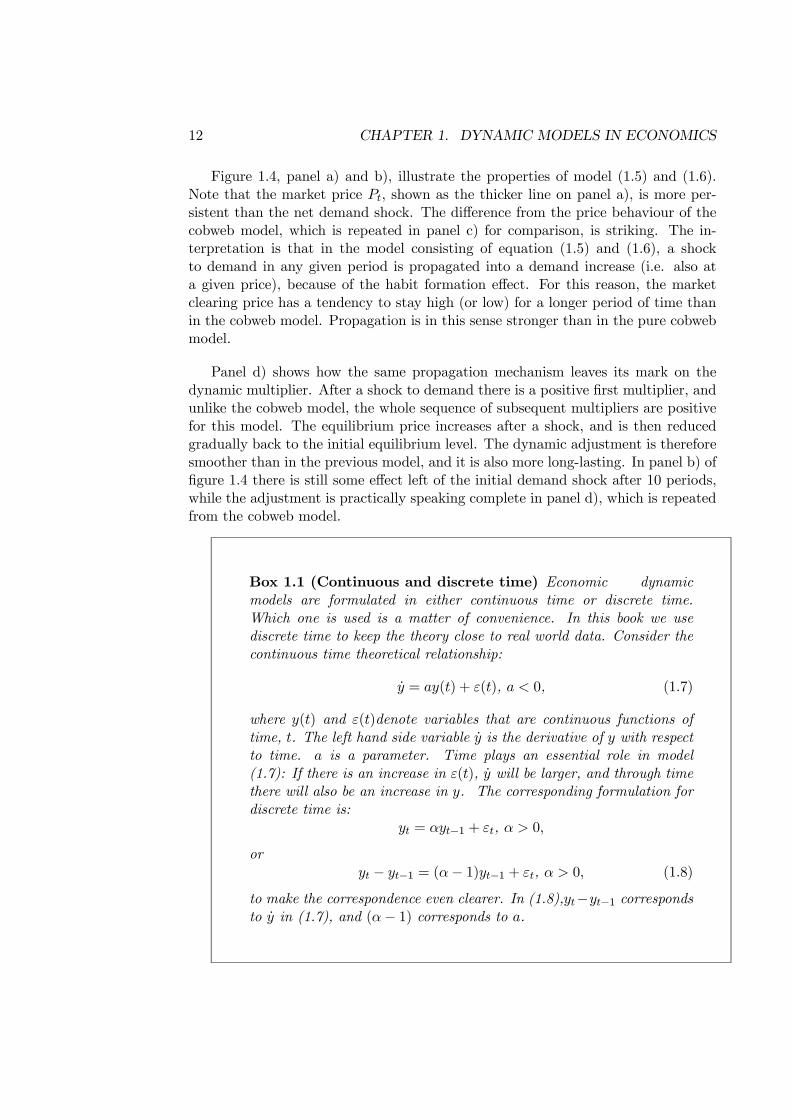
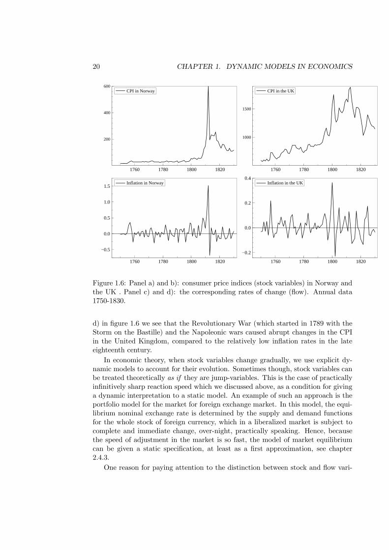
A typical empirical trait of stock variables is that they change gradually, as a sum-mation of often quite small growth rates. Occasionally however, a stock variablejumps from one level in period t to another level in period t + 1. In theory, withcontinuous time, see Box 1.1 below, the derivative of the variable with respect totime is infinite at the time of the jump. In practice, with discrete time data, therate of change becomes relatively large in such instances. In the Norwegian “pricehistory” the high rate of change in the consumer price index at the time of thebreakdown of the union with Denmark may be regarded an empirical example ofjump behaviour in the price level, since the annual rate of inflation increased fromapproximately 25% to 150%, see figure 1.6, panel a) and c). From panel b) and
20 CHAPTER 1. DYNAMIC MODELS IN ECONOMICS
1760 1780 1800 1820
200
400
600CPI in Norway
1760 1780 1800 1820
1000
1500
CPI in the UK
1760 1780 1800 1820
−0.5
0.0
0.5
1.0
1.5Inflation in Norway
1760 1780 1800 1820
−0.2
0.0
0.2
0.4Inflation in the UK
Figure 1.6: Panel a) and b): consumer price indices (stock variables) in Norway andthe UK . Panel c) and d): the corresponding rates of change (flow). Annual data1750-1830.
d) in figure 1.6 we see that the Revolutionary War (which started in 1789 with theStorm on the Bastille) and the Napoleonic wars caused abrupt changes in the CPIin the United Kingdom, compared to the relatively low inflation rates in the lateeighteenth century.
In economic theory, when stock variables change gradually, we use explicit dy-namic models to account for their evolution. Sometimes though, stock variables canbe treated theoretically as if they are jump-variables. This is the case of practicallyinfinitively sharp reaction speed which we discussed above, as a condition for givinga dynamic interpretation to a static model. An example of such an approach is theportfolio model for the market for foreign exchange market. In this model, the equi-librium nominal exchange rate is determined by the supply and demand functionsfor the whole stock of foreign currency, which in a liberalized market is subject tocomplete and immediate change, over-night, practically speaking. Hence, becausethe speed of adjustment in the market is so fast, the model of market equilibriumcan be given a static specification, at least as a first approximation, see chapter2.4.3.
One reason for paying attention to the distinction between stock and flow vari-
1.6. STOCK AND FLOW VARIABLES 21
1980 1985 1990 1995 2000
0
25
50
75 The Norwegian current account
Bill
ion
kron
er
1980 1985 1990 1995 2000
-750
-500
-250
0
Norwegian net foreign debt
Bill
ion
kron
er
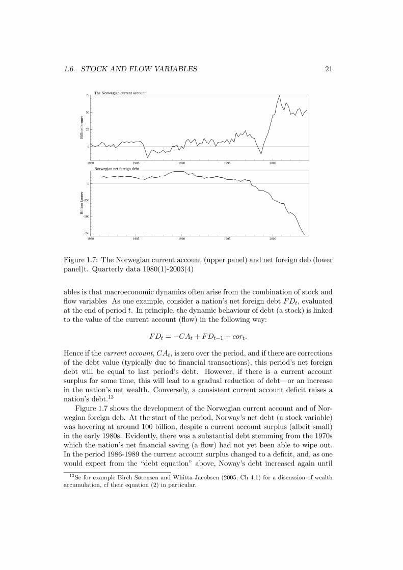
Figure 1.7: The Norwegian current account (upper panel) and net foreign deb (lowerpanel)t. Quarterly data 1980(1)-2003(4)
ables is that macroeconomic dynamics often arise from the combination of stock andflow variables As one example, consider a nation’s net foreign debt FDt, evaluatedat the end of period t. In principle, the dynamic behaviour of debt (a stock) is linkedto the value of the current account (flow) in the following way:
FDt = −CAt + FDt−1 + cort.
Hence if the current account, CAt, is zero over the period, and if there are correctionsof the debt value (typically due to financial transactions), this period’s net foreigndebt will be equal to last period’s debt. However, if there is a current accountsurplus for some time, this will lead to a gradual reduction of debt–or an increasein the nation’s net wealth. Conversely, a consistent current account deficit raises anation’s debt.13
Figure 1.7 shows the development of the Norwegian current account and of Nor-wegian foreign deb. At the start of the period, Norway’s net debt (a stock variable)was hovering at around 100 billion, despite a current account surplus (albeit small)in the early 1980s. Evidently, there was a substantial debt stemming from the 1970swhich the nation’s net financial saving (a flow) had not yet been able to wipe out.In the period 1986-1989 the current account surplus changed to a deficit, and, as onewould expect from the “debt equation” above, Noway’s debt increased again until
13Se for example Birch Sørensen and Whitta-Jacobsen (2005, Ch 4.1) for a discussion of wealthaccumulation, cf their equation (2) in particular.
22 CHAPTER 1. DYNAMIC MODELS IN ECONOMICS
it peaked in 1990. Later in the 1990s, the current account surplus returned, andtherefore the net debt was gradually reduced. Later, at the end of the millennium,surpluses grew to unprecedented magnitudes, up to 75 billion per quarter, resultingin a sharp build up of net financial wealth, accumulating to 750 billion kroner at theend of the period.
Section 2.4.3 discusses the role of the current account in the theory of the marketfor foreign exchange, in particular why it is fruitful to distinguish between stock andflow variables in the analysis of that market.
The theory of economic growth provides another example of the importance ofstock and flow dynamics. For example, the level of production (a flow variable) in theeconomy depends on the size of the labour stock (literary speaking), and the capitalstock. Due to the phenomenon of capital depreciation, some of today’s productionneeds to be saved just in order to keep the capital stock intact in the first period ofthe future. Moreover, due to population growth (and a declining marginal productof labour), next period’s capital stock will have to be larger than it is today if wewant to avoid that output per capita declines in the next period. Hence, economicgrowth in terms of GDP per head requires that the flow of net investment (grossinvestment minus capital depreciation) is positive. In line with this, the dynamicequation of the capital stock is written as
Kt+1 = Kt + Jt −Dt
where Kt denotes the capital stock at the start of period t, Jt is the flow of grossinvestment during period t, and Dt is replacement investment (also a flow). A muchused assumption is that Dt is proportional to the pre-existing capital stock, i.e.,Dt = δKt where the rate of capital depreciation δ is a positive number which is lessthan or equal to one. This gives a well known expression for the development of thecapital stock
Kt+1 = (1− δ)Kt + Jt, 0 < δ ≤ 1, (1.13)
which plays an important role in growth theory (see chapter 2.8.3), in real businesscycle theory (see chapter 2.8.4), and generally in all macro models with endogenouscapital accumulation.
Another case of stock-flow dynamics is the relationship between wages and un-employment, which we will discuss in detail in chapter 3. The rate of unemploymentis a stock variable which influences wage growth (a flow variable) and inflation inthe form of the relative change in CPI.. On the other hand, the rate of unemploy-ment depends on accumulated wage growth which determines the real wage level (astock variable). Similar linkages exist between nominal and real exchange rates, andprovide one of the key dynamic mechanisms in the models of the national economythat we encounter in macroeconomics.
1.7. SUMMARY AND OVERVIEW OF THE REST OF THE BOOK 23
1.7 Summary and overview of the rest of the book
The quotation from Norges Bank’s web pages at the beginning of the chapter showsthat the Central Bank has formulated a view about the dynamic effects of a changein the interest rate on inflation. In the quotation, the Central Bank states that theeffect will take place within two years, i.e., 8 quarters in a quarterly model of therelationship between the rate of inflation and the rate of interest. That statementmay be taken to mean that the effect is building up gradually over 8 quarters andthen dies away quite quickly, but other interpretations are also possible. In orderto inform the public more fully about its view on the monetary policy transmissionmechanism, the Bank would have to give a more detailed picture of the dynamiceffects of a change in the interest rate. Similar issues arise whenever it is of interestto study how fast and how strongly an exogenous perturbation or a policy changeaffect the economy, for example how private consumption is likely to be affected bya certain amount of tax-cut.
Chapter 2 is an introduction to the modelling tools of dynamic analysis. Buildingon the motivation of this chapter, we present a general framework for dynamicsingle equation models, called the autoregressive distributed lag model, or ADL forshort. In terms of mathematics, the ADL model corresponds to linear differenceequations, but we assume no knowledge of the mathematics of difference equationsin this course. Instead, this important model class is motivated by its relevancefor economic dynamics, and by the intuitive economic interpretation of the model’sparameters.
Having introduced the ADLmodel, we can use that model that model to establishformally the properties of the dynamic multiplier, which we in fact have come acrossseveral times already in the introduction, for example in the analysis of the cobwebmodel. The observant reader may already have gauged that the dynamic multiplieris a key concept in this course, and once you get a good grip on it, you have apowerful tool which allows you to calculate the dynamic effects of policy changes(and of other exogenous shocks for that matter) in a dynamic model. The ADLmodel also defines a typology of dynamic equations, as special cases, each with theirdistinct features and economic meaning. One particular transformation of the ADLmodel is the error correction model, is particularly useful, since it shows explicitlyhow dynamic models combines variables that are in terms of changes with respectto time (differenced data), with the past levels of the variables. Finally in chapter2, the analysis is extended to simple dynamic systems-of-equations. For both thesingle equations and for systems-of-equations, a number of macroeconomic examplesand applications are discussed in details.
In chapter 3 the analytical tools of chapter 2 are applied to wage-and-price set-ting, which is an essential part of the supply side of modern macroeconomic model.A main difference from existing textbooks is that our approach rationalizes that thecareful modelling of bargaining based wage setting leads to a representation of thesupply side model which cannot be subsumed in a standard Phillips curve relation-ship. This changes the premises for stabilization policy as currently perceived. In
24 CHAPTER 1. DYNAMIC MODELS IN ECONOMICS
later versions these models of the supply side will be integrated in a model of theopen macroeconomy.
Exercises
1. Consider the model consisting of equation (1.3) and (1.4). Experiment withdifferent slopes of the demand and (long-run) supply functions, correspondingto different values of the parameters a and c, and check whether the cobwebis always “spiraling inwards”. Or can other patterns emerge?
2. In equation (1.4), what it the derivative of supply in period t, Xt, with respectto price in period t? What is the derivative of Xt+1 with respect to Pt?Interpret your results in the light of the graph in figure 1.3.
3. In the model defined by equation (1.5) and (1.6), what is the expression forthe slope of the long-run demand curve? What happens to the slope if b = 1,and can you think of an interpretation of this case?
4. Modify the model in (1.5) and (1.6) by introducing an exogenous variable Zt,representing total consumption expenditure, in the demand equation. Assumethat initiallyZt is at a constant level z0 in all time periods. Try to illustrateand explain the effects of a negative expenditure shock that lasts for 2 periodsbefore Z goes back to z0 and stays there.
Chapter 2
Linear dynamic models
Section 2.1 introduces an important class of dynamic models calledthe autoregressive distributed lag model (ADL), and the concept of thedynamic multiplier, already encountered in the first chapter, is madeprecise within that framework. A typology of dynamic equations whithrelevance in macroeconomics is presented in section 2.3, and section 2.4gives examples of how economic models and hypothesis can be formu-lated in the framework of the ADL. Section 2.5 and 2.6 show that staticand dynamic equations can be reconciled, and integrated, by the use ofthe equilibrium correction model, ECM, which in turn is a “1-1” trans-formation of the ADL. In section 2.7 we discuss the solution of dynamicmodels. Finally, section 2.8 sketches how the analysis can be extendedto multi equation dynamic models (dynamic systems). Two examples ofmacroeconomic systems: the Solow growth model and the real businesscycle model, are reviewed in some detail.
2.1 The autoregressive distributed lag model and dy-namic multipliers
In chapter 1 we gave examples of dynamic relationships, for example the supplyequation of the cobweb model. We also introduced the concept of dynamic multiplier,which is the dynamic response of an endogenous variable to a shock to the model.In this section we present a model known as the autoregressive distributed lag model.It is a single equation model with only first order dynamics – so it is quite simple.Nevertheless, the model is general enough to allow us to explain all the essentialproperties of linear dynamic models in a precise way.
In equation (2.1), yt is the endogenous variable while xt is the exogenous variable:
yt = β0 + β1xt + β2xt−1 + αyt−1 + εt. (2.1)
Since x enters both with its current value, xt, and its lagged value xt−1 is is custom tosay that x enters the equation as a distributed lag. β0 and β1 are the distributed lag
25
26 CHAPTER 2. LINEAR DYNAMIC MODELS
coefficients. Higher order distributed lags are often used in practical applications,but for our purpose we loose nothing by concentrating on the simplest case with afirst order distributed lag.
The first lag of yt – called the autoregressive term – also appears on the righthand of equation (2.1). yt−1 is multiplied by the coefficient α, which is called theautoregressive coefficient. In the same way as in the first chapter, εt symbolizesthe small and random part of yt which is unexplained by xt, xt−1 and yt−1. It iscommon to refer to εt as the shock variable in the dynamic equation. Since themodel combines a distributed lag in the exogenous variable with an autoregressiveterm, the name autoregressive distributed lag model (ADL for short) is much used.
In many applications economic, as in the consumption function example below,y and x are in logarithmic scale. However, in other applications, different units ofmeasurement are the natural ones to use. Thus, depending of which variables we aremodelling, y and x can be measured in million kroner, or in thousand persons, orin percentage points. Combinations of measurement are also often used in practice:for example in studies of labour demand, yt may denote the number of hours workedin the economy, while xt denotes real wage costs per hour and is therefore measuredin kroner. The measurement scale does not affect the mathematical derivation ofthe dynamic multipliers below, but care must be taken when interpreting the re-sults. Specifically, only when both y and x are in logs, are the multipliers directlyinterpretable as percentage changes in y following a 1% increase in x, i.e., they are(dynamic) elasticities.
We now show that dynamic multipliers correspond to the derivatives of yt, yt+1,yt+2, ...., with respect to changes in x. We draw a distinction between a temporarychange in x and a permanent change in x. By a temporary change we mean anincrease in x that lasts for only one period – in the following period, x returnsto its initial value and stays there forever. In the case of a permanent change, xincreases to a new level and stays there forever. Since we work with a linear model,all results that we establish for positive changes applies equally to negative changes,just by changing the signs of the dynamic effects.
2.1.1 The effects of a temporary change: dynamic multipliers
We first derive the dynamic effects on y of at temporary change in x. These effectsare called dynamic multipliers. By definition, a temporary change in period t affectsonly xt, not xt+1 or any other x’s further into the future. Hence from (2.1) wehave directly that the first dynamic multiplier, which it is custom to call the impactmultiplier is
∂yt∂xt
= β1.
The second dynamic multiplier is found by considering the equation for period t+1,namely:
yt+1 = β0 + β1xt+1 + β2xt + αyt + εt+1. (2.2)
2.1. THE AUTOREGRESSIVE DISTRIBUTED LAGMODEL ANDDYNAMICMULTIPLIERS 27
The partial derivative of (2.2) with respect to xt is
∂yt+1∂xt
= β2 + α∂yt∂xt
,
and is the second dynamic multiplier. It is often referred to as the interim multiplierfor the first lag. To find the third dynamic multiplier, consider
yt+2 = β0 + β1xt+2 + β2xt+1 + αyt+1 + εt+2, (2.3)
and take the derivative to obtain the interim multiplier for the second lag.
∂yt+2∂xt
= α∂yt+1∂xt
= α2β1 + αβ2.
In general, for period t+ j we have
yt+j = β0 + β1xt+j + β2xt+j−1 + αyt+j−1 + εt+j ,
and the interim multiplier for lag j = 1 is∂yt+j∂xt
= α∂yt+j−1∂xt
= αjβ1 + αj−1β2, (2.4)
showing that, as long as −1 < α < 1, each dynamic multiplier is smaller in magni-tude than the previous. The multipliers are therefore zero asymptotically , formally:
∂yt+j∂xt
−→j−→∞
0, if and only if − 1 < α < 1. (2.5)
The expressions for the dynamic multipliers are collected in the second column oftable 2.1.
2.1.2 The effects of a permanent change: cumulated interim mul-tipliers
In economics we often whish to find the effects on y of a permanent change in theexplanatory variable. It is then convenient to think of xt, xt+1, xt+2, , .... as increas-ing functions of a continuous variable h. When h changes permanently, starting inperiod t,we have ∂xt+j/∂h > 0, for j = 0, 1, 2, ..., while there is no change in xt−1and yt−1 since those two variables are predetermined. Since xt is a function of h, sois yt, and the effect of yt of the change in h is found as
∂yt∂h
= β1∂xt∂h
.
In the outset, ∂xt/∂h can be any number but because it is convenient, is has becomecustom to evaluate the multipliers for the case of ∂xt/∂h = 1 which is referred asthe case of a unit-change. Following this practice, the first multiplier is
∂yt∂h
= β1. (2.6)
28 CHAPTER 2. LINEAR DYNAMIC MODELS
It should come as no surprise that this is the same as the first multiplier in the caseof a temporary change in x.
The second multiplier associated with a permanent change in x is found using(2.2) and calculating the derivative ∂yt+1/∂h. Since our premise is that the changein h occurs in period t, both xt+1 and xt are changed. We need to keep in mindthat yt is a function of h, hence:
∂yt+1∂h
= β1∂xt+1∂h
+ β2∂xt∂h
+ α∂yt∂h
(2.7)
Again, considering a unit-change, ∂xt/∂h = ∂xt+1/∂h = 1, and using (2.6), thesecond multiplier can be written as
∂yt+1∂h
= β1 + β2 + α∂yt∂h
= β1(1 + α) + β2. (2.8)
Using equation (2.3) and the same logic as the second multiplier, we obtain
∂yt+2∂h
= β1∂xt+2∂h
+ β2∂xt+1∂h
+ α∂yt+1∂h
(2.9)
= β1 + β2 + α∂yt+1∂h
= β1(1 + α+ α2) + β2(1 + α)
as the expression for the third multiplier. Note that the conventional unit-change,∂xt/∂h = ∂xt+1/∂h = 1, has been used in the second line, and the third line is theresult of substituting ∂yt+1/∂h by the right hand side of (2.8).
Comparison of equation (2.7) with the first line of (2.9) shows that there isa clear pattern: The third and second multipliers are linked by exactly the sameform of dynamics that govern yt itself. This also holds for higher order multipliers,and means that these multipliers can be computed recursively : For example, oncewe have found the third multiplier, the fourth can be found easily by substituting∂yt+2/∂h on the right hand side of
∂yt+3∂h
= β1 + β2 + α∂yt+2∂h
(2.10)
with the expression in the final line of equation (2.9).In table 2.1, the column named Permanent unit change in xt collects the results
we have obtained. In the table, to save space, we use the notation δj (j = 0, 1, 2, ...)for the sequence of multipliers caused by a permanent change in x. For, example δ0is identical to ∂yt/∂h in (2.6), and δ1 is identical to the second multiplier, ∂yt+1/∂hin (2.8), and so on. Because the multipliers are linked together in a recursive pattern,multiplier j + 1 is given by
δj = β1 + β2 + αδj−1, for j = 1, 2, 3, . . . (2.11)
2.1. THE AUTOREGRESSIVE DISTRIBUTED LAGMODEL ANDDYNAMICMULTIPLIERS 29
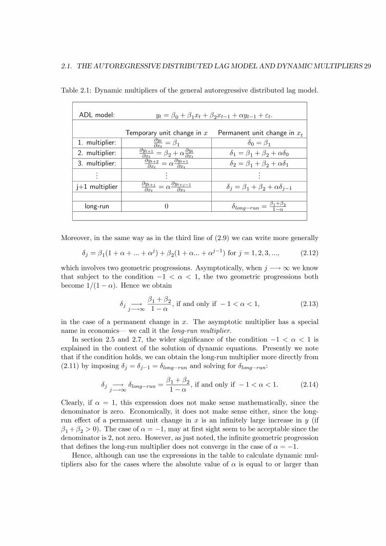
Table 2.1: Dynamic multipliers of the general autoregressive distributed lag model.
ADL model: yt = β0 + β1xt + β2xt−1 + αyt−1 + εt.
Temporary unit change in x Permanent unit change in xt1. multiplier: ∂yt
∂xt= β1 δ0 = β1
2. multiplier: ∂yt+1∂xt
= β2 + α ∂yt∂xt
δ1 = β1 + β2 + αδ0
3. multiplier: ∂yt+2∂xt
= α∂yt+1∂xt
δ2 = β1 + β2 + αδ1...
......
j+1 multiplier ∂yt+j∂xt
= α∂yt+j−1∂xt
δj = β1 + β2 + αδj−1
long-run 0 δlong−run =β1+β21−α
Moreover, in the same way as in the third line of (2.9) we can write more generally
δj = β1(1 + α+ ...+ αj) + β2(1 + α...+ αj−1) for j = 1, 2, 3, ..., (2.12)
which involves two geometric progressions. Asymptotically, when j −→∞ we knowthat subject to the condition −1 < α < 1, the two geometric progressions bothbecome 1/(1− α). Hence we obtain
δj −→j−→∞
β1 + β21− α
, if and only if − 1 < α < 1, (2.13)
in the case of a permanent change in x. The asymptotic multiplier has a specialname in economics– we call it the long-run multiplier.
In section 2.5 and 2.7, the wider significance of the condition −1 < α < 1 isexplained in the context of the solution of dynamic equations. Presently we notethat if the condition holds, we can obtain the long-run multiplier more directly from(2.11) by imposing δj = δj−1 = δlong−run and solving for δlong−run:
δj −→j−→∞
δlong−run =β1 + β21− α
, if and only if − 1 < α < 1. (2.14)
Clearly, if α = 1, this expression does not make sense mathematically, since thedenominator is zero. Economically, it does not make sense either, since the long-run effect of a permanent unit change in x is an infinitely large increase in y (ifβ1+β2 > 0). The case of α = −1, may at first sight seem to be acceptable since thedenominator is 2, not zero. However, as just noted, the infinite geometric progressionthat defines the long-run multiplier does not converge in the case of α = −1.
Hence, although can use the expressions in the table to calculate dynamic mul-tipliers also for the cases where the absolute value of α is equal to or larger than
30 CHAPTER 2. LINEAR DYNAMIC MODELS
unity, the long-run multiplier of a permanent change in x does not exist in this case.Correspondingly: the multipliers of a temporary change do not converge to zero inthe case where −1 < α < 1 does not hold.
Notice that, unlike α = 1, the case of α = 0 does not represent a problem. Thisrestriction, which is seen to exclude the autoregressive term yt−1 from the model,only serves to simplify the dynamic multipliers, and it is referred to by economistsas the distributed lag model, denoted DL-model, as in the equation typology below.
Heuristically, the effect of a permanent change in the x’s can be viewed as thesum of the changes triggered by a temporary change in period t. Indeed, there is analgebraic relationship between the interim multipliers and the dynamic multipliersassociated with a permanent change. To see this, note that the 2nd multiplier δ1 intable 2.1 is
δ1 = β1 + β2 + αβ1
which is the same at the sum of the impact multiplier and the first interim multiplier:
∂yt∂xt
+∂yt+1∂xt
= β1 + β2 + αβ1 = (1 + α)β1 + β2 ≡ δ1
The third dynamic multiplier is the sum of the impact multiplier and the two nextinterim multipliers:
∂yt∂xt
+∂yt+1∂xt
+∂yt+2∂xt
= β1 + β2 + αβ1 + α(β2 + αβ1)
= (1 + α+ α2)β1 + (1 + α)β2 ≡ δ2
and generally, for the j’th dynamic multiplier:
δj =Xj
k=0
∂yt+k∂xt
= (1 + α+ ...+ αj)β1 + (1 + α+ ...+ αj−1)β2, j = 1, 2, ....
In reflection of these algebraic relationships, the dynamic multipliers due to a per-manent change in the x’s, are often referred to as the cumulated interim multipliers.Similarly, the long-run multiplier δlong−run can be rationalized as the infinite sumof the interim multipliers, subject to the condition that −1 < α < 1.
In a way, the interim multipliers associated with a temporary change are themore fundamental of the two types of dynamic multiplies that we have considered:If we first calculate the effects of a temporary shock, the dynamic effects of a per-manent shock can be calculated afterwards by summation of the impact and interimmultipliers.
2.2 An example: dynamic effects of increased incomeon consumption
In this section we discuss an empirical example where yt is (the logarithm) of privateconsumption, and we consider in detail a dynamic model of consumption where the
2.2. AN EXAMPLE: DYNAMIC EFFECTS OF INCREASED INCOMEONCONSUMPTION31
explanatory variable xt is the log of private disposable income. When we considereconomic models to be used in an analysis of real world macro data, care must betaken to distinguish between static and dynamic models. The textbook consumptionfunction, i.e., the relationship between real private consumption expenditure (C) andreal households’ disposable income (INC) is an example of a static equation
Ct = f(INCt), f 0 > 0. (2.15)
Consumption in any period t is strictly increasing in income, hence the positivesigned first order derivative f 0 which is called the marginal propensity to consume.To be able to apply the theory to observations of the real economy we also haveto specify the function f(INCt). Two of the most used functional forms in macro-economics, are the linear and log-linear specifications. For the case of the staticconsumption function in (2.15), these two specifications are
Ct = β0 + β1INCt + et, (linear), and (2.16)
lnCt = β0 + β1 ln INCt + et, (log-linear). (2.17)
For simplicity we use the same symbols for the coefficients in the two equations.However, it is important to note that since the variables are measured on differentscales–million kroner at fixed prices in (2.16), the natural logarithm of fixed millionkroner in (2.17)–the slope coefficient β1 has a different economic interpretation inthe two models.1
Thus, in equation (2.16), β1 is the marginal propensity to consume and is inunits of million kroner. Mathematically, β1 in (2.16) is the derivative of real privateconsumption, Ct with respect to real income, INCt:
dCt
dINCt= β1, from (2.16).
In the log linear model (2.17), since both real income and real consumption aretransformed by applying the natural logarithm to each variable, it is common to saythat each variable have been “log-transformed”. By taking the differential of thelog-linear consumption function we obtain (see appendix A for a short reference onlogarithms):
dCt
Ct= β1
dINC
INCtor
dCt
dINCt
INCt
Ct= β1.
1 In practice, this means that if LCt is private consumption expenditure in million (or billion)kroner in period t, Ct is defined as LCt/PCt where PCt is the price deflator in period t. If, forexample, Ct is in million 2000 kroner, this means that the base year of the consumer price indexPCt is 2000 (with annual data, PC2000 = 1, with quarterly data, the annual average is 1 in 2000).Yt is defined accordingly.
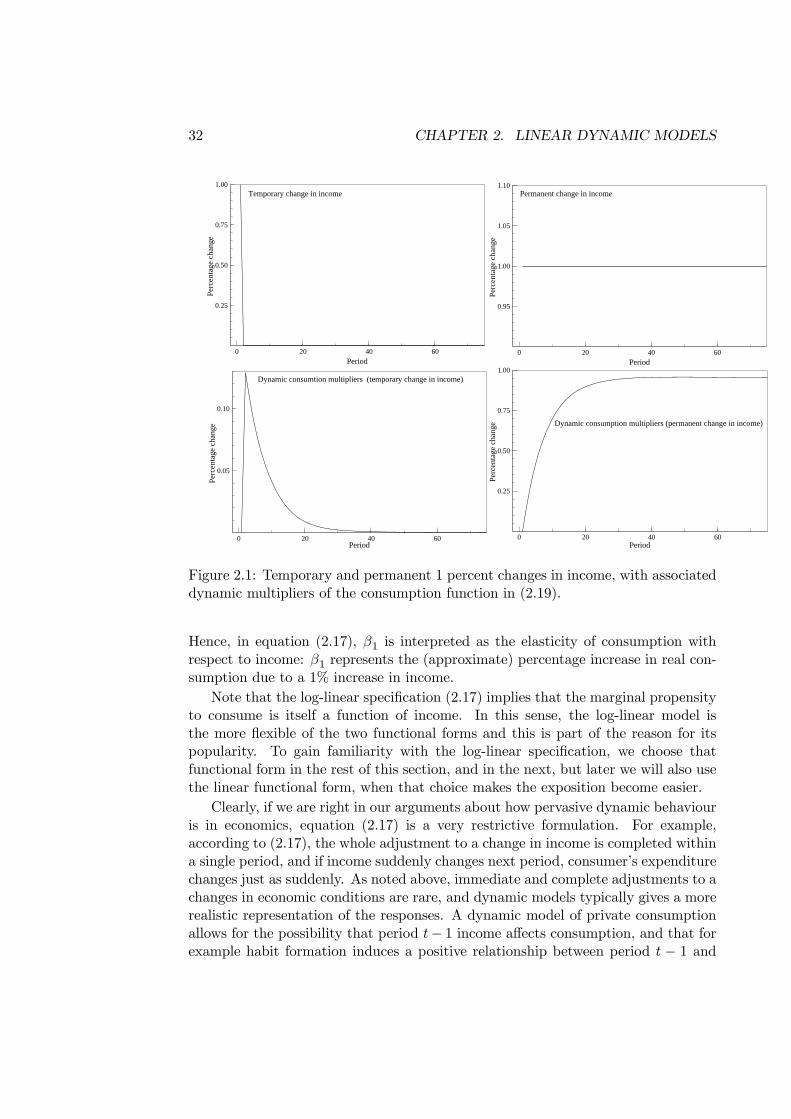
32 CHAPTER 2. LINEAR DYNAMIC MODELS
0 20 40 60
0.05
0.10
Dynamic consumtion multipliers (temporary change in income)
Perc
enta
ge c
hang
e
Period
0 20 40 60
0.25
0.50
0.75
1.00Temporary change in income
Perc
enta
ge c
hang
e
Period
0 20 40 60
0.25
0.50
0.75
1.00
Dynamic consumption multipliers (permanent change in income)
Perc
enta
ge c
hang
e
Period
0 20 40 60
0.95
1.00
1.05
1.10Permanent change in income
Perc
enta
ge c
hang
e
Period
Figure 2.1: Temporary and permanent 1 percent changes in income, with associateddynamic multipliers of the consumption function in (2.19).
Hence, in equation (2.17), β1 is interpreted as the elasticity of consumption withrespect to income: β1 represents the (approximate) percentage increase in real con-sumption due to a 1% increase in income.
Note that the log-linear specification (2.17) implies that the marginal propensityto consume is itself a function of income. In this sense, the log-linear model isthe more flexible of the two functional forms and this is part of the reason for itspopularity. To gain familiarity with the log-linear specification, we choose thatfunctional form in the rest of this section, and in the next, but later we will also usethe linear functional form, when that choice makes the exposition become easier.
Clearly, if we are right in our arguments about how pervasive dynamic behaviouris in economics, equation (2.17) is a very restrictive formulation. For example,according to (2.17), the whole adjustment to a change in income is completed withina single period, and if income suddenly changes next period, consumer’s expenditurechanges just as suddenly. As noted above, immediate and complete adjustments to achanges in economic conditions are rare, and dynamic models typically gives a morerealistic representation of the responses. A dynamic model of private consumptionallows for the possibility that period t− 1 income affects consumption, and that forexample habit formation induces a positive relationship between period t − 1 and
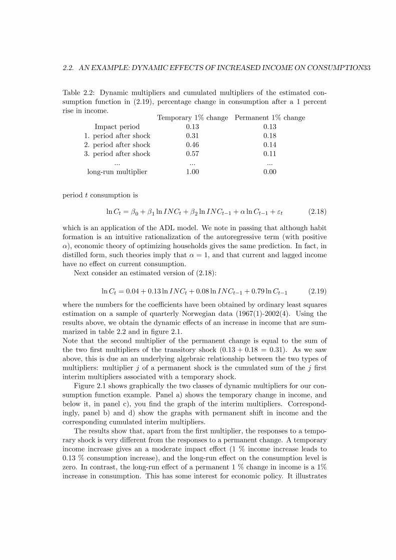
2.2. AN EXAMPLE: DYNAMIC EFFECTS OF INCREASED INCOMEONCONSUMPTION33
Table 2.2: Dynamic multipliers and cumulated multipliers of the estimated con-sumption function in (2.19), percentage change in consumption after a 1 percentrise in income.
Temporary 1% change Permanent 1% changeImpact period 0.13 0.13
1. period after shock 0.31 0.182. period after shock 0.46 0.143. period after shock 0.57 0.11
... ... ...long-run multiplier 1.00 0.00
period t consumption is
lnCt = β0 + β1 ln INCt + β2 ln INCt−1 + α lnCt−1 + εt (2.18)
which is an application of the ADL model. We note in passing that although habitformation is an intuitive rationalization of the autoregressive term (with positiveα), economic theory of optimizing households gives the same prediction. In fact, indistilled form, such theories imply that α = 1, and that current and lagged incomehave no effect on current consumption.
Next consider an estimated version of (2.18):
lnCt = 0.04 + 0.13 ln INCt + 0.08 ln INCt−1 + 0.79 lnCt−1 (2.19)
where the numbers for the coefficients have been obtained by ordinary least squaresestimation on a sample of quarterly Norwegian data (1967(1)-2002(4). Using theresults above, we obtain the dynamic effects of an increase in income that are sum-marized in table 2.2 and in figure 2.1.Note that the second multiplier of the permanent change is equal to the sum ofthe two first multipliers of the transitory shock (0.13 + 0.18 = 0.31). As we sawabove, this is due an an underlying algebraic relationship between the two types ofmultipliers: multiplier j of a permanent shock is the cumulated sum of the j firstinterim multipliers associated with a temporary shock.
Figure 2.1 shows graphically the two classes of dynamic multipliers for our con-sumption function example. Panel a) shows the temporary change in income, andbelow it, in panel c), you find the graph of the interim multipliers. Correspond-ingly, panel b) and d) show the graphs with permanent shift in income and thecorresponding cumulated interim multipliers.
The results show that, apart from the first multiplier, the responses to a tempo-rary shock is very different from the responses to a permanent change. A temporaryincome increase gives an a moderate impact effect (1 % income increase leads to0.13 % consumption increase), and the long-run effect on the consumption level iszero. In contrast, the long-run effect of a permanent 1 % change in income is a 1%increase in consumption. This has some interest for economic policy. It illustrates
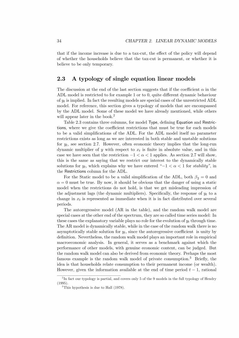
34 CHAPTER 2. LINEAR DYNAMIC MODELS
that if the income increase is due to a tax-cut, the effect of the policy will dependof whether the households believe that the tax-cut is permanent, or whether it isbelieve to be only temporary.
2.3 A typology of single equation linear models
The discussion at the end of the last section suggests that if the coefficient α in theADL model is restricted to for example 1 or to 0, quite different dynamic behaviourof yt is implied. In fact the resulting models are special cases of the unrestricted ADLmodel. For reference, this section gives a typology of models that are encompassedby the ADL model. Some of these model we have already mentioned, while otherswill appear later in the book.2
Table 2.3 contains three columns, for model Type, defining Equation and Restric-tions, where we give the coefficient restrictions that must be true for each modelsto be a valid simplifications of the ADL. For the ADL model itself no parameterrestrictions exists as long as we are interested in both stable and unstable solutionsfor yt, see section 2.7. However, often economic theory implies that the long-rundynamic multiplier of y with respect to xt is finite in absolute value, and in thiscase we have seen that the restriction −1 < α < 1 applies. As section 2.7 will show,this is the same as saying that we restrict our interest to the dynamically stablesolutions for yt, which explains why we have entered “−1 < α < 1 for stability”, inthe Restrictions column for the ADL.
For the Static model to be a valid simplification of the ADL, both β2 = 0 andα = 0 must be true. By now, it should be obvious that the danger of using a staticmodel when the restrictions do not hold, is that we get misleading impression ofthe adjustment lags (the dynamic multipliers). Specifically, the response of yt to achange in xt is represented as immediate when it is in fact distributed over severalperiods.
The autoregressive model (AR in the table), and the random walk model arespecial cases at the other end of the spectrum, they are so called time series model: Inthese cases the explanatory variable plays no role for the evolution of yt through time.The AR model is dynamically stable, while in the case of the random walk there is noasymptotically stable solution for yt, since the autoregressive coefficient is unity bydefinition. Nevertheless, the random walk model plays an important role in empiricalmacroeconomic analysis. In general, it serves as a benchmark against which theperformance of other models, with genuine economic content, can be judged. Butthe random walk model can also be derived from economic theory. Perhaps the mostfamous example is the random walk model of private consumption.3 Briefly, theidea is that households relate consumption to their permanent income (or wealth).However, given the information available at the end of time period t − 1, rational
2 In fact our typology is partial, and covers only 5 of the 9 models in the full typology of Hendry(1995).
3This hypothesis is due to Hall (1978).
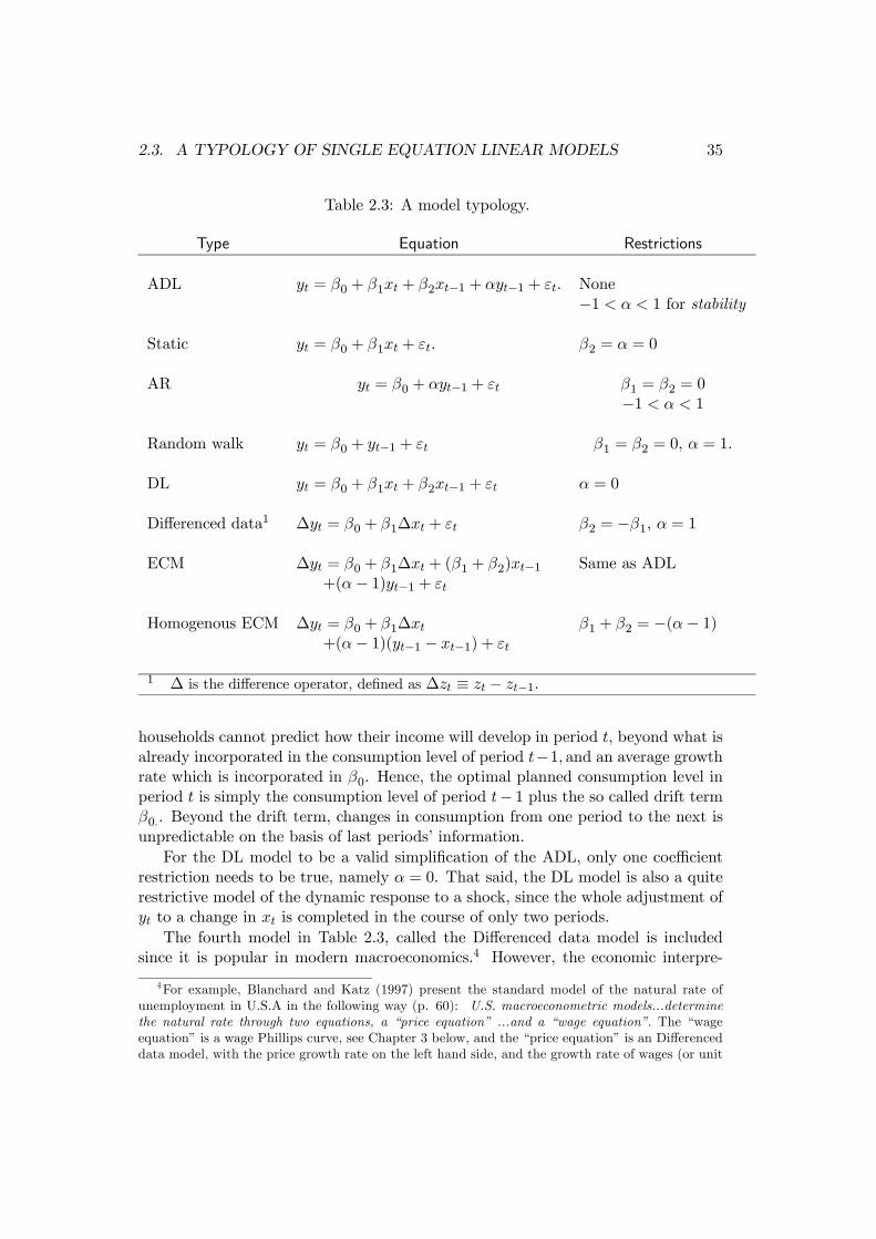
2.3. A TYPOLOGY OF SINGLE EQUATION LINEAR MODELS 35
Table 2.3: A model typology.
Type Equation Restrictions
ADL yt = β0 + β1xt + β2xt−1 + αyt−1 + εt. None−1 < α < 1 for stability
Static yt = β0 + β1xt + εt. β2 = α = 0
AR yt = β0 + αyt−1 + εt β1 = β2 = 0−1 < α < 1
Random walk yt = β0 + yt−1 + εt β1 = β2 = 0, α = 1.
DL yt = β0 + β1xt + β2xt−1 + εt α = 0
Differenced data1 ∆yt = β0 + β1∆xt + εt β2 = −β1, α = 1
ECM ∆yt = β0 + β1∆xt + (β1 + β2)xt−1 Same as ADL+(α− 1)yt−1 + εt
Homogenous ECM ∆yt = β0 + β1∆xt β1 + β2 = −(α− 1)+(α− 1)(yt−1 − xt−1) + εt
1 ∆ is the difference operator, defined as ∆zt ≡ zt − zt−1.
households cannot predict how their income will develop in period t, beyond what isalready incorporated in the consumption level of period t−1, and an average growthrate which is incorporated in β0. Hence, the optimal planned consumption level inperiod t is simply the consumption level of period t− 1 plus the so called drift termβ0.. Beyond the drift term, changes in consumption from one period to the next isunpredictable on the basis of last periods’ information.
For the DL model to be a valid simplification of the ADL, only one coefficientrestriction needs to be true, namely α = 0. That said, the DL model is also a quiterestrictive model of the dynamic response to a shock, since the whole adjustment ofyt to a change in xt is completed in the course of only two periods.
The fourth model in Table 2.3, called the Differenced data model is includedsince it is popular in modern macroeconomics.4 However, the economic interpre-
4For example, Blanchard and Katz (1997) present the standard model of the natural rate ofunemployment in U.S.A in the following way (p. 60): U.S. macroeconometric models...determinethe natural rate through two equations, a “price equation” ...and a “wage equation”. The “wageequation” is a wage Phillips curve, see Chapter 3 below, and the “price equation” is an Differenceddata model, with the price growth rate on the left hand side, and the growth rate of wages (or unit
36 CHAPTER 2. LINEAR DYNAMIC MODELS
tation of the Differenced data model (‘growth rate model’ if yt and xt are in logs)is problematic, since behaviour according to this models can only be rationalizedif there are no cost of being out of equilibrium in terms of the levels variables ytand xt.5 At present, this implication may not be obvious, but it section 2.5 it willbe explained when we review the properties of the two last models in Table 2.3,the error-correction model, ECM,and the Homogeneous ECM. These two models donot have the shortcomings of the Static, DL or Differenced data models. Specif-ically, the ECM, is consistent with a long-run relationship between y and x, andit also describes the behaviour of yt outside equilibrium. As explained in section2.5 below, the ECM is a re-parameterization of the dynamically stable ADL, hencenone other restrictions applies to the ECM than to the dynamically stable ADL.The Homogenous ECM has the same advantages as the ECM in terms of economicinterpretation, but the long-run multiplier is restricted to unity.
As noted, restricting the long-run multiplier to unity is not generic to the ECM,but is implied by some economic theories. One example is so called Purchasing PowerParity (PPP) theory, in which case yt is the log of the domestic price index (mostoften the CPI), and xt is the log of an index of foreign prices, denoted in domesticcurrency. The hypothesis of purchasing power parity states that the elasticity of thedomestic price level with respect to the foreign price level is unity, and the mostrealistic implementation of the PPP hypothesis is to set β1 + β2 = (1 − α) whichimplies δlong−run = 1, as we have seen. In section 2.6, a different interpretationof the PPP hypothesis is discussed as well. Other examples of Homogenous ECMsmotivated by economic theory include consumption functions that are consistentwith a constant long-run saving rate, and theories of wage setting that imply thatthe wage-share is constant in the long-run, as discussed in Chapter 3.
The ADL model in equation (2.1) is general enough to serve as an introductionto most aspects of dynamic analysis in economics. However, the ADL model, andthe dynamic multiplier analysis, can be extended in several directions to provideadditional flexibility in applications. The most important extensions are:
1. Several explanatory variables
2. Longer lags
3. Systems of dynamics equations
In economics, more than one explanatory variable is usually needed to provide asatisfactory explanation of the behaviour of a variable yt. The ADL model (2.1) can
labour costs) on the right hand side.5A more technical motivation for the Differenced data model is that, by taking the difference
of yt and xt prior to estimation, the econometric problem of residual autocorrelation is reduced.However, unless the two restrictions that define the model are empirically acceptable, choosing theDifferenced data model rather than the ADL model creates more problems than it solves. Forexample, the regression coefficient of ∆xt will neither be a correct estimate of the impact multiplierβ1, nor of the long-run multiplier δlong−run. Neverthless, estimation of models with only differenceddata, often large systems which are dubbed differenced data vector autoregressive models (dVAR)has become stanadard in applied macroeconomics.
2.3. A TYPOLOGY OF SINGLE EQUATION LINEAR MODELS 37
be generalized to any number of explanatory variables. However, nothing is lost interms of understanding by only considering the case of two exogenous variables, x1,tand x2,t. The extension of equation (2.1) to this case is
yt = β0 + β11x1t + β21x1t−1+ (2.20)
β12x2t + β22x2t−1 + αyt−1 + εt,
where βik is the coefficient of the i0th lag of the explanatory variable k. The dynamic
multipliers of yt can be with respect to either x1 of x2, the derivation being exactlythe same as above. Formally, we can think of each set of multipliers as correspond-ing to partial derivatives. In applications, the dynamic multipliers of the differentexplanatory variables are often found to be markedly different. For example, if ytis the (log of) the hourly wage, while x1 and x2 are the rate of unemployment andproductivity respectively, dynamic multipliers with respect to unemployment is usu-ally much smaller in magnitude than the multipliers with respect to productivity forreasons that are explained in chapter 3.
Longer lags in either the x’s or in the autoregressive part of the model makesfor more flexible dynamics. Even though the dynamics of such models can be quitecomplicated, the dynamic multipliers always exist, and can be computed by followingthe logic of section ?? above. However, as such calculation quickly become tiring, weuse computer software when we work with such models (good econometric softwarepackages includes options for dynamic multiplier analysis). In this course, we do notconsider the formal analysis of higher order autoregressive dynamics.
Often, an ADL equation is joined up with other equations to form dynamicsystem of equations. For example, assume that x2t is an exogenous explanatoryvariable in (2.20) but that x1,t is an endogenous variable. This implies that (2.20) issupplemented by a second equation which has x1t on the left hand side and with ytas one of the variables on the right hand side. Hence, x1t and yt are determined in asimultaneous two equation system. Another, equally relevant example, is where theequation for x1t contains the lag yt−1, but not the contemporaneous yt. Also in thiscase are x2t and yt jointly determined, in what is referred to as a recursive systemof equations. In either case the true multipliers of yt with respect to the exogenousvariable x2t, cannot be derived from equation (2.20) alone, because that would makeus miss the feed-back that a change in x2,t has on yt via the endogenous variablex1,t. To obtain the correct dynamic multipliers of y with respect to x1 we must usethe two equation system.
Many more economic examples of dynamic systems, and of how they can be usedin analysis, will crop up as we proceed. In particular, section 2.8 takes the dynamicversion of the Keynesian multiplier models as one specific example, and the Solowgrowth model, and a Real Business Cycle model as two other examples. In fact, thereader will have noticed that already in Chapter 1 we analyzed a dynamic systemof supply and demand in a single-market, without any formalism though. Otherapplications of dynamic systems are found in the chapters on wage-price dynamicsand on economic policy analysis.
38 CHAPTER 2. LINEAR DYNAMIC MODELS
2.4 More examples of dynamic relationships in economics
The ADL model covers a wide range of economic models, in fact all theories that canbe expressed as linear models of causal or future-independent processes. A causalprocess is characterized by its solution (see section 2.7) at time t being independentof future values of the explanatory variable and of the disturbance. Hence futurevalues {xt+1, xt+2, ...} and {εt+1, εt+2,..} do not affect affect the solution for yt.Although causal models are practical, and therefore widely used in economics andin other disciplines, macroeconomics make use of non-causal models as well. Theextension of dynamics to non-causal processes, where the dynamically stable solutionfor yt depends on {xt+1, xt+2, ...} and {εt+1, εt+2,..} stems from the forward-lookingbehaviour which is assumed in many modern theories. In chapter 3.6, we present theNew Keynesian Phillips Curve, which is a model of price adjustment that illustratemany of the typical traits of non-causal models. In this section we give examples ofstandard models that are covered by the causal ADL model.
2.4.1 The dynamic consumption function (revisited)
The consumption function with both consumption and income in logs has been theour example so far. Of course, exactly the same analysis and algebra apply to alinear functional form of the consumption function, except that the multipliers willbe in units of million kroner (at fixed prices) rather than percentages. In section 2.8below the linear consumption function is combined with the general budget equationto form a dynamic system.
In modern econometric work on the consumption function, more variables areusually included than just income. Hence, there are other multipliers to considerthan the ones with respect to INCt. The most commonly found additional ex-planatory variables are wealth, the real interest rate and indicators of demographicdevelopments, see Erlandsen and Nymoen (2008).
2.4.2 The price Phillips curve
In Chapter 3, and several times later in the book, we will consider the so calledexpectations augmented Phillips curve. An example of such a relationship is
πt = β0 + β11ut + β12ut−1 + β21πet+1 + εt. (2.21)
πt denotes the rate of inflation, πt = ln(Pt/Pt−1), where Pt is an index of the pricelevel of the economy. ut is the rate of unemployment–or its natural logarithm.The distinction between ut as the unemployment rate (or percentage), or the logof the rate of unemployment is an example of the care that needs to be taken inchoice between different functional forms. If ut is a rate (as with the unemploymentpercentage), the Phillips curve is linear, and the effect of a small change in ut on πtis independent of the initial unemployment percentage.
2.4. MORE EXAMPLES OF DYNAMIC RELATIONSHIPS IN ECONOMICS 39
If on the other hand ut is defined as ut = ln(the rate of unemployment), thePhillips curve is non-linear. In that case, and starting from a low level, a rise inthe rate of unemployment leads to a larger reduction in πt than if the initial rateof unemployment is high. The graph of the price Phillips curve, with the rateof unemployment on the horizontal axis, is curved towards the origin (a convexfunction).6 In many countries, a convex Phillips curve is known to give a betterfit to the data than the linear function. In these economies, a policy that aims atcontrolling inflation indirectly, via the rate of unemployment, has a better chance ofsuccess if the initial level of unemployment is relatively low, compared to the casewhere the rate of unemployment is relatively high. Thus we see that an apparentlytechnical detail, namely the choice of functional form, has important implicationsfor the effectiveness of policy. This is important to keep this in mind when we laterin the this book, for reasons of exposition, often choose to define ut as the rate ofunemployment.
In equation (2.21), the distributed lag in the rate of unemployment capturesseveral interesting economic hypotheses. For example, if the rise in inflation followinga fall in unemployment is first weak but then gets stronger, we might have that bothβ11 < 0 and β12 < 0. On the other hand, some economist have argued the opposite:that the inflationary effects of changes in unemployment are likely to be strongestin the first periods after shock to unemployment, in which case we might expect tofind that β11 < 0 while β12 > 0.
Finally, in equation (2.21), πet+1 denotes the expected rate of inflation one periodahead, and in the same manner as earlier in this chapter, εt denotes a randomdisturbance term. In sum, (2.21) includes two explanatory variables: the rate ofunemployment, and the expectation of the future value of the endogenous variable.The rate of unemployment is observable, but expectations are usually not. In orderto make progress from (2.21) it is therefore necessary to specify a hypothesis ofexpectations. The simplest hypothesis is that expectations build on the last observedrate of inflation, hence
πet+1 = τπt−1, (2.22)
where the parameter τ is typically positive, but not larger than 1, i.e., 0 < τ ≤ 1.7Substitution of πet+1 by (2.22), the Phillips curve in (2.21) becomes
πt = β0 + β11ut + β12ut−1 + απt−1 + εt, (2.23)
which is an ADL equation (with α = β21τ).
6On Norwegian data, wage Phillips curves, and also the error correction models of wage formationthat we encounter below, have alternatively included a reciprocal term, i.e., 1/ut, where ut is therate of unemployment, or even the double reciprocal 1/u2t . This functional form is “more non-linear”than the log-form. Beyond a certain level of unemployment, there is no more inflation reduction tobe hauled from further increases of unemployment, see Johansen (1995).
7This fits real word data for the case where we think of πt as the annual rate of inflation. Withmonthly or quarterly observations of the rate of inflation, seasonal variation calls for more flexibledynamics (more lags) than in (2.21) and/or (2.22).
40 CHAPTER 2. LINEAR DYNAMIC MODELS
As explained, the hypothesis in equation (2.22) is just one out of many possibleformulations about expectations formation. Alternative specifications give rise toother dynamic models of the rate of inflation. Consider for example a situationwhere the government have introduced an explicit inflation target, which we denoteπ. In this case, it is reasonable to believe that firms and households will base theirexpectations of future inflation on the attainment of the inflation target. In thesimplest case we may then set
πet+1 = π (2.24)
in place of (2.22). As an exercise, you should convince yourself that equations (2.21)and (2.24) imply an equation for inflation which is an example of a distributed lagmodel (DL model). More generally, firms and households take into considerationthe possibility that future inflation is not exactly on target. Hence they may adopta more robust forecasting rule, for example
πet+1 = (1− τ)π + τπt−1, 0 < τ ≤ 1. (2.25)
In this case, the derived dynamic equation for inflation again takes the form of anADL model.
2.4.3 Exchange rate dynamics
The market for foreign exchange plays a central role in open economy macroeco-nomics. As always in commodity markets there is a demand and supply side. Inthe market for foreign exchange, the good in question is foreign currency. Withoutloss of generality, we can focus on a single country and assume that there is a singleforeign country. The price of the good–the nominal exchange rate–is then theprice of the foreign currency in terms of the currency of the domestic country. Forsimplicity we can for example refer to the foreign currency as US dollars, or euro,and to the domestic currency as kroner. The exchange rate is then the price ofdollars (or euros) in kroner, for example 7 kroner per dollar.8
In the theory of the foreign exchange market a change of emphasis has takenplace in recent years. The standard open economy macro model used to treat thenet supply of currency to the domestic central bank as a flow variable, primarily de-termined by the current account. In times of a current account surplus for example,there is an excess supply of currency to the central bank. Hence, in the flow model ofthe market for foreign exchange, a positive net supply of foreign currency, explainedby a surplus on the current account, is expected to lead to currency appreciation (inthe case of a floating exchange rate regime).
The modern approach to the foreign exchange market does not deny that theneeds for currency exchange of exporters and importers make out a part of the netsupply of foreign exchange. However, it is a fact that in modern open economiesmost of the trade in foreign currency is capital movements. Domestic and foreign
8We refer to Rødseth (2000, Ch 1 and 3.1) for an excellent exposition of the portfolio model ofthe market for foreign exchange.
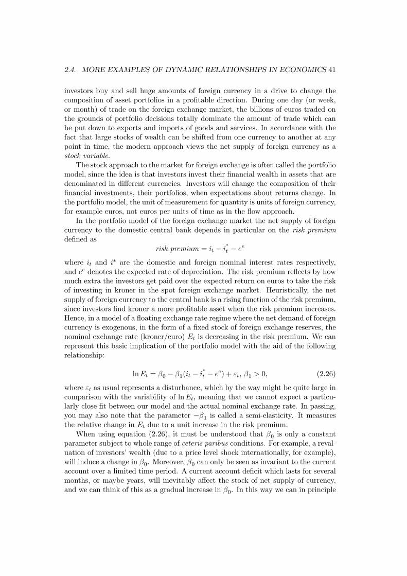
2.4. MORE EXAMPLES OF DYNAMIC RELATIONSHIPS IN ECONOMICS 41
investors buy and sell huge amounts of foreign currency in a drive to change thecomposition of asset portfolios in a profitable direction. During one day (or week,or month) of trade on the foreign exchange market, the billions of euros traded onthe grounds of portfolio decisions totally dominate the amount of trade which canbe put down to exports and imports of goods and services. In accordance with thefact that large stocks of wealth can be shifted from one currency to another at anypoint in time, the modern approach views the net supply of foreign currency as astock variable.
The stock approach to the market for foreign exchange is often called the portfoliomodel, since the idea is that investors invest their financial wealth in assets that aredenominated in different currencies. Investors will change the composition of theirfinancial investments, their portfolios, when expectations about returns change. Inthe portfolio model, the unit of measurement for quantity is units of foreign currency,for example euros, not euros per units of time as in the flow approach.
In the portfolio model of the foreign exchange market the net supply of foreigncurrency to the domestic central bank depends in particular on the risk premiumdefined as
risk premium = it − i∗t − ee
where it and i∗ are the domestic and foreign nominal interest rates respectively,and ee denotes the expected rate of depreciation. The risk premium reflects by howmuch extra the investors get paid over the expected return on euros to take the riskof investing in kroner in the spot foreign exchange market. Heuristically, the netsupply of foreign currency to the central bank is a rising function of the risk premium,since investors find kroner a more profitable asset when the risk premium increases.Hence, in a model of a floating exchange rate regime where the net demand of foreigncurrency is exogenous, in the form of a fixed stock of foreign exchange reserves, thenominal exchange rate (kroner/euro) Et is decreasing in the risk premium. We canrepresent this basic implication of the portfolio model with the aid of the followingrelationship:
lnEt = β0 − β1(it − i∗t − ee) + εt, β1 > 0, (2.26)
where εt as usual represents a disturbance, which by the way might be quite large incomparison with the variability of lnEt, meaning that we cannot expect a particu-larly close fit between our model and the actual nominal exchange rate. In passing,you may also note that the parameter −β1 is called a semi-elasticity. It measuresthe relative change in Et due to a unit increase in the risk premium.
When using equation (2.26), it must be understood that β0 is only a constantparameter subject to whole range of ceteris paribus conditions. For example, a reval-uation of investors’ wealth (due to a price level shock internationally, for example),will induce a change in β0. Moreover, β0 can only be seen as invariant to the currentaccount over a limited time period. A current account deficit which lasts for severalmonths, or maybe years, will inevitably affect the stock of net supply of currency,and we can think of this as a gradual increase in β0. In this way we can in principle
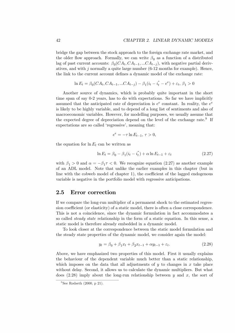
42 CHAPTER 2. LINEAR DYNAMIC MODELS
bridge the gap between the stock approach to the foreign exchange rate market, andthe older flow approach. Formally, we can write β0 as a function of a distributedlag of past current accounts: β0(CAt, CAt−1, ...CAt−j), with negative partial deriv-atives, and with j normally a quite large number (6-12 months for example). Hence,the link to the current account defines a dynamic model of the exchange rate:
lnEt = β0(CAt, CAt−1, ...CAt−j)− β1(it − i∗t − ee) + εt, β1 > 0
Another source of dynamics, which is probably quite important in the shorttime span of say 0-2 years, has to do with expectations. So far we have implicitlyassumed that the anticipated rate of depreciation is ee constant. In reality, the ee
is likely to be highly variable, and to depend of a long list of sentiments and also ofmacroeconomic variables. However, for modelling purposes, we usually assume thatthe expected degree of depreciation depend on the level of the exchange rate.9 Ifexpectations are so called ‘regressive’, meaning that:
ee = −τ lnEt−1, τ > 0,
the equation for lnEt can be written as
lnEt = β0 − β1(it − i∗t ) + α lnEt−1 + εt (2.27)
with β1 > 0 and α = −β1τ < 0. We recognize equation (2.27) as another exampleof an ADL model. Note that unlike the earlier examples in this chapter (but inline with the cobweb model of chapter 1), the coefficient of the lagged endogenousvariable is negative in the portfolio model with regressive anticipations.
2.5 Error correction
If we compare the long-run multiplier of a permanent shock to the estimated regres-sion coefficient (or elasticity) of a static model, there is often a close correspondence.This is not a coincidence, since the dynamic formulation in fact accommodates aso called steady state relationship in the form of a static equation. In this sense, astatic model is therefore already embedded in a dynamic model.
To look closer at the correspondence between the static model formulation andthe steady state properties of the dynamic model, we consider again the model:
yt = β0 + β1xt + β2xt−1 + αyt−1 + εt. (2.28)
Above, we have emphasized two properties of this model. First it usually explainsthe behaviour of the dependent variable much better than a static relationship,which imposes on the data that all adjustments of y to changes in x take placewithout delay. Second, it allows us to calculate the dynamic multipliers. But whatdoes (2.28) imply about the long-run relationship between y and x, the sort of
9See Rødseth (2000, p 21).
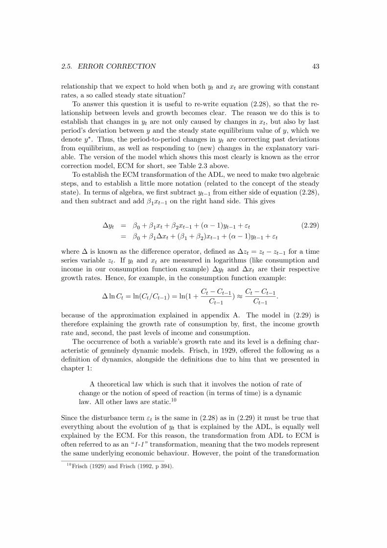
2.5. ERROR CORRECTION 43
relationship that we expect to hold when both yt and xt are growing with constantrates, a so called steady state situation?
To answer this question it is useful to re-write equation (2.28), so that the re-lationship between levels and growth becomes clear. The reason we do this is toestablish that changes in yt are not only caused by changes in xt, but also by lastperiod’s deviation between y and the steady state equilibrium value of y, which wedenote y∗. Thus, the period-to-period changes in yt are correcting past deviationsfrom equilibrium, as well as responding to (new) changes in the explanatory vari-able. The version of the model which shows this most clearly is known as the errorcorrection model, ECM for short, see Table 2.3 above.
To establish the ECM transformation of the ADL, we need to make two algebraicsteps, and to establish a little more notation (related to the concept of the steadystate). In terms of algebra, we first subtract yt−1 from either side of equation (2.28),and then subtract and add β1xt−1 on the right hand side. This gives
∆yt = β0 + β1xt + β2xt−1 + (α− 1)yt−1 + εt (2.29)
= β0 + β1∆xt + (β1 + β2)xt−1 + (α− 1)yt−1 + εt
where ∆ is known as the difference operator, defined as ∆zt = zt − zt−1 for a timeseries variable zt. If yt and xt are measured in logarithms (like consumption andincome in our consumption function example) ∆yt and ∆xt are their respectivegrowth rates. Hence, for example, in the consumption function example:
∆ lnCt = ln(Ct/Ct−1) = ln(1 +Ct − Ct−1
Ct−1) ≈ Ct − Ct−1
Ct−1.
because of the approximation explained in appendix A. The model in (2.29) istherefore explaining the growth rate of consumption by, first, the income growthrate and, second, the past levels of income and consumption.
The occurrence of both a variable’s growth rate and its level is a defining char-acteristic of genuinely dynamic models. Frisch, in 1929, offered the following as adefinition of dynamics, alongside the definitions due to him that we presented inchapter 1:
A theoretical law which is such that it involves the notion of rate ofchange or the notion of speed of reaction (in terms of time) is a dynamiclaw. All other laws are static.10
Since the disturbance term εt is the same in (2.28) as in (2.29) it must be true thateverything about the evolution of yt that is explained by the ADL, is equally wellexplained by the ECM. For this reason, the transformation from ADL to ECM isoften referred to as an “1-1” transformation, meaning that the two models representthe same underlying economic behaviour. However, the point of the transformation10Frisch (1929) and Frisch (1992, p 394).
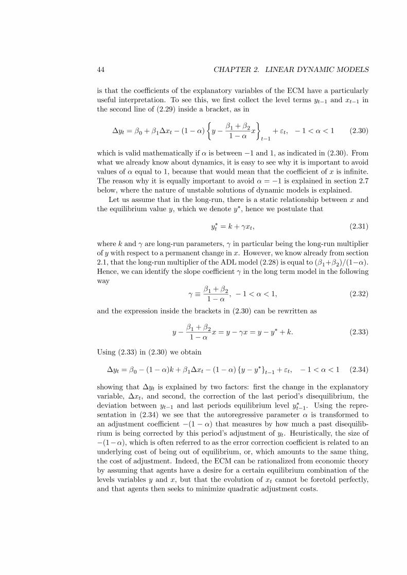
44 CHAPTER 2. LINEAR DYNAMIC MODELS
is that the coefficients of the explanatory variables of the ECM have a particularlyuseful interpretation. To see this, we first collect the level terms yt−1 and xt−1 inthe second line of (2.29) inside a bracket, as in
∆yt = β0 + β1∆xt − (1− α)
½y − β1 + β2
1− αx
¾t−1
+ εt, − 1 < α < 1 (2.30)
which is valid mathematically if α is between −1 and 1, as indicated in (2.30). Fromwhat we already know about dynamics, it is easy to see why it is important to avoidvalues of α equal to 1, because that would mean that the coefficient of x is infinite.The reason why it is equally important to avoid α = −1 is explained in section 2.7below, where the nature of unstable solutions of dynamic models is explained.
Let us assume that in the long-run, there is a static relationship between x andthe equilibrium value y, which we denote y∗, hence we postulate that
y∗t = k + γxt, (2.31)
where k and γ are long-run parameters, γ in particular being the long-run multiplierof y with respect to a permanent change in x. However, we know already from section2.1, that the long-run multiplier of the ADL model (2.28) is equal to (β1+β2)/(1−α).Hence, we can identify the slope coefficient γ in the long term model in the followingway
γ ≡ β1 + β21− α
, − 1 < α < 1, (2.32)
and the expression inside the brackets in (2.30) can be rewritten as
y − β1 + β21− α
x = y − γx = y − y∗ + k. (2.33)
Using (2.33) in (2.30) we obtain
∆yt = β0 − (1− α)k + β1∆xt − (1− α) {y − y∗}t−1 + εt, − 1 < α < 1 (2.34)
showing that ∆yt is explained by two factors: first the change in the explanatoryvariable, ∆xt, and second, the correction of the last period’s disequilibrium, thedeviation between yt−1 and last periods equilibrium level y∗t−1. Using the repre-sentation in (2.34) we see that the autoregressive parameter α is transformed toan adjustment coefficient −(1 − α) that measures by how much a past disequilib-rium is being corrected by this period’s adjustment of yt. Heuristically, the size of−(1−α), which is often referred to as the error correction coefficient is related to anunderlying cost of being out of equilibrium, or, which amounts to the same thing,the cost of adjustment. Indeed, the ECM can be rationalized from economic theoryby assuming that agents have a desire for a certain equilibrium combination of thelevels variables y and x, but that the evolution of xt cannot be foretold perfectly,and that agents then seeks to minimize quadratic adjustment costs.
2.5. ERROR CORRECTION 45
With reference to Table 2.3, we note that the Homogenous ECM has exactlythe same properties and interpretation as the ordinary ECM, but that the long-run multiplier γ is unity according to some relevant economic theory of the long-run relationship between xt and yt. The other models in the typology in contrastentail restrictions on the speed of adjustment, and on the cost of being out of levelsequilibrium.
We next consider a theoretical steady state situation in which growth rates areconstants, ∆xt = gx, ∆yt = gy, and the disturbance term is equal to its averagevalue of zero, εt = 0. Imposing this in (2.34), and noting that {y − y∗}t−1 = 0 bydefinition of a steady state, gives
gy = β0 + β1gx − (1− α)k,
meaning that the constant term in the long-term relationship (2.31) can be expressedas
k =−gy + β0 + β1gx
1− α, (2.35)
again subject to a condition −1 < α < 1. Often we only consider a static steadystates, with no growth, so gy = gx = 0. In that case k is simply β0/(1− α).
In sum, there is an important correspondence between the dynamic model anda static relationship like (2.31) motivated by economic theory:
1. A theoretical linear relationship y∗ = k + γx can be retrieved as the steadystate solution of the dynamic model (2.28). This generalizes to theory modelswith more than one explanatory variable (e.g., y∗ = k + γ1x1 + γ2x2) as longas both x1t and x2t (and/or their lags) are included in the dynamic model.In chapter 3 we will discuss some details of this extension in the context ofmodels of wage and price setting (inflation).
2. The theoretical slope coefficient γ is identical to the corresponding long-runmultiplier (of a permanent increase in the respective explanatory variables).
3. Conversely, if we are only interested in quantifying a long-run multiplier (ratherthan the whole sequence of dynamic multipliers), it can be found by using theidentity in (2.32).
Returning to another insight in this section, we note that the transformation of theADL model into levels and differences is often referred to as “the error correctiontransformation”. The name reflects that according to the model, ∆yt corrects pastdeviation from the long-run equilibrium relationship. Error correction models be-came popular in econometrics in the early 1980s. Since ∆yt is actually bringingthe level of y towards the long-run relationship, a better name may be equilibriumcorrection model, and some authors now use that term consistently, see Hendry(2008). The acronym ECM is used for both error correction model and equilibriumcorrection model. .
46 CHAPTER 2. LINEAR DYNAMIC MODELS
The ECM, not only helps clarify the link between dynamics and the theoreticalsteady state, it also plays an essential role in econometric modelling of non-stationarytime series. In 2003, when Clive Granger and Rob Engle were awarded the NoblePrice in economics, this was in part due to their finding that so called cointegrationbetween two or more non-stationary variables implies error correction, and viceversa.
In common usage, the term error correction model is not only used about equa-tion (2.30), where the long-run relationship is explicit, but also about (the secondline) of (2.29). One reason is that the long-run multipliers (the coefficients of thelong-run relationship) can be easily established by estimating the linear relationshipin (2.30), and then calculating the ratio γ in (2.32). Direct estimation of γ requiresa non-linear estimation method.
2.6 The two interpretations of static equations
In the first chapter we discussed the definitional differences between static mod-els and dynamic models. One of the conclusions was that there are two differentinterpretations of static relationships in macroeconomics:
1. As representations of actual behaviour in macroeconomics, and
2. as corresponding to long-run, steady state, relationships.
In terms of the concepts we have developed in this chapter, the first interpretationcorresponds to simplifying the ADL model
yt = β0 + β1xt + β2xt−1 + αyt−1 + εt.
by setting β2 = 0 and α = 0 as in the Static model in the typology in table 2.3. In thisinterpretation, a static model are seen to be a special case of the ADL model. Sincethere are no reason to believe a priori that the two parameters are empirically foundto be zero very often, the static special case is also a restrictive model relative to theADL. In economic terminology, and as we have noted in the first chapter, the validityof the static model hinges on the assumption that the speed of adjustment is so fastthat explicit dynamics can be omitted from the model. In more operational termswe may perhaps put it this way: Sometimes, we can assume (either because it isrealistic or because we are willing to simplify) that the dynamic adjustment processis so fast that the adjustment to a change in an exogenous variable is completedwithin the period of analysis. Hence, at least as a first approximation, we do notneed to formulate the dynamic adjustment process explicitly.
One example of this rationale for a static model is the simple Keynesian income-expenditure model. As the reader will know, this model is based on an assumptionof fixed wages and prices. When we use the income expenditure model, the focusis on the aggregate short-run effects of for example a rise in government expen-diture, and for this purpose, the results of the analysis is believed not to be seri-ously distorted by the abstraction from price-wage dynamics, which in industrialized
2.6. THE TWO INTERPRETATIONS OF STATIC EQUATIONS 47
economies normally is more sluggish than the response in employment and output.It is understood that the relevance of this rationalization depends on the compar-ative and historical context, and on the stage of evolution of the economy which isthe subject to the analysis. Broadly speaking, the assumption is only realistic foreconomies where the short-run aggregate supply curve is relatively horizontal–fortechnological and/or institutional reasons. The model is not relevant for historicalor contemporary agricultural economies for example, or for industrialized economiesthat have been damaged by wars or by the collapse of institutions, and which there-fore have become hyper-inflation economies. The Weimar republic in Germany afterthe First World War is an important historical example. Zimbabwe between 1998and 2008 is a contemporary example–and there are many more.
If the time horizon of the analysis is longer than 1-2 years, the assumption offixed wage and price levels becomes untenable, also in the case of well functioningindustrialized economies. The loss of relevance from ignoring for example the effectsof inflation on the real interest rate and on the rate of foreign exchange, is alsoincreasing with the time horizon of the analysis. Hence, the explicit modelling ofwage and price dynamics is necessary if the model is to be relevant for fiscal andmonetary policy analysis over the business cycle, i.e., a 5 to 10 year period. Chapter3 therefore gives a comprehensive introduction to dynamic models of wage and priceformation.
The second interpretation of a static model allows β2 and a to take values differ-ent from zero, and in fact only hinges on α being “different from one”. This secondinterpretation of static models is exactly the interpretation that we have developedso far in this chapter, and in section 2.5 on the ECM in particular. This interpreta-tion applies to all asymptotically stable dynamic models, where a model’s impliedsteady state relationships represents an equilibrium situation. That equilibrium canbe represented mathematically with the aid of static (timeless) equations of the typegiven above. Frisch’s formulation from 1929 already contained this interpretation ofstatic models as long-relationships:
Therefore static laws basically express what would happen in thelong-run if the static theory’s assumptions prevailed long enough for thephenomena to have time to have time to react in accordance with theseassumptions.11
Clearly, to avoid confusion, the two interpretations of a static model should not bemixed-up. Nevertheless, the two interpretation are often confounded, and it is notuncommon that static equations are first presented as long-run relationship, butthen, at some point in the argument the same relationship is used as a short-runmodel, often in a rather complicated system-of-equations. In chapter 3, we showthat a standard way of rationalizing a modern Phillips curve relationship suffersfrom lack of precision in this respect.
11Frisch (1992, p 395), Frisch’s italics.
48 CHAPTER 2. LINEAR DYNAMIC MODELS
Another example which shows that care must be taken when we choose an oper-ational interpretation of generally formulated economic hypotheses, is provided bythe theory of Purchasing Power Parity, PPP. This hypothesis is about the behaviourthe real exchange rate, σ, which is defined as
σ =EP ∗
P
where P ∗ represents the foreign price level, E is the nominal exchange rate (kro-ner/euro) and P is the domestic price level. The purchasing power parity condition(PPP) used in many macroeconomic models says that “the real exchange rate isconstant”.12 This is trivial if the empirical counterparts of E, P ∗ and P , i.e. theobservable time series Et, P ∗t and Pt, are constant, but even a casual glance at thedata shows that they are not. So, to be able to put the PPP hypothesis to use(or to test), we must ask about the time perspective of the PPP condition. If it istaken as a short-run proposition, he real exchange rate is constant from one periodto the next, σt = σt−1 = k. In the case of exogenous Et, like in a fixed exchangerate regime, and with an exogenous foreign price level, PPP is seen to imply thefollowing model of the domestic price level Pt:
lnPt = − ln k + lnEt + lnP∗t , (2.36)
a static price equation, which says that the effect of a currency change in periodt on the domestic price level is full and immediate in period t. Hence, in thisinterpretation, the short-run elasticities of the domestic price level with respect toits determinants, Et and P ∗t , are identical and equal to the long-run elasticities. Allelasticities are unity. In the exchange rate literature, this case is referred to as thecase of full and immediate pass-through.
If on the other hand, PPP is interpreted as a long-run proposition, we haveinstead the interpretation that σt = σ in a steady state situation, and thus
∆ lnPt = gE + π∗ (2.37)
where gE and π∗ denote the long-run constant growth rates of the nominal exchangerate and of foreign prices. In this interpretation there is full long-run pass-through,but the PPP hypothesis has no implications for the short-run pass-through, i.e. forthe dynamic multipliers. However, (2.37) is often confounded with the relationship
∆ lnPt = ∆ lnEt +∆ lnP∗t
which is a Differenced data model in terms of the typology in table 2.3, and so holdsno implication for the long-run dynamics.
12For a concise introduction to the purchasing power parity, see Rødseth (2000, p 261).
2.7. SOLUTION AND SIMULATION OF DYNAMIC MODELS 49
2.7 Solution and simulation of dynamic models
The reader will have noted that the existence of a finite long-run multiplier, andthereby the validity of the correspondence between the ADL model and long-runrelationships, depends on the autoregressive parameter α in (2.28) being differentfrom unity. In section 2.7.1 we show that the parameter α is also crucial for thenature and type of solution of equation (2.28). Several of the insights obtained byconsidering the solution of the ADL equation (2.28) in some detail, carry over tomore complicated equations as well as to systems of equations.
2.7.1 The solution of ADL equations
In order to discuss the solution of ADL models, it is useful to first consider thesimpler case of a deterministic autoregressive model, where we abstract from thedistributed lag part (xt and xt−1) of the model, as well as from the disturbanceterm (εt). One way to achieve this simplification of (2.28) is to assume that both xtand εt are fixed at their respective constant averages:
εt = 0 for t = 1, ..., and
xt = mx for t = 0, 1....
Hence we follow convention and assume that each εt, representing a small and ran-dom influence on y, has a common mean of zero. For the explanatory variable xtthe mean is denoted mx. We write the simplified model as
yt = β0 + (β1 + β2)mx + αyt−1, for t = 1, 2, ..... (2.38)
In the following we proceed as if the the coefficients β0, β1, β2 and α are knownnumbers. This is a simplifying assumption which allows us to abstract from estima-tion issues, which in any case belong to a course in time series econometrics.
We assume that equation (2.38) holds for t = 1, 2, .... It is usual to refer to t = 0as the initial period or the initial condition. The assumption we make about theinitial period is crucial for the existence and uniqueness of a solution. An importanttheorem is the following: If y0 is a fixed and known number, then there is a uniquesequence of numbers y0, y1, y2, ... which is the solution of (2.38). This can be seen byinduction: Consider first t = 0: From the assumption of known initial conditions, y0then follows. Next, set t = 1 in (2.38), and y1 is seen to determined uniquely sincewe already know y0. And so on: having established yt−1 we find yt be solving (2.38)one period forward. This procedure is also known as solving the equation recursivelyfrom known initial conditions.
You may note that, unlike other “conditions for solution” in other areas of math-ematical economics, the requirement of fixed and known initial conditions is almosttrivial, since y0 is simply given “from history”. If we open up for the possibilitythat the initial condition is not determined by history, but that it can “jump” at
50 CHAPTER 2. LINEAR DYNAMIC MODELS
any point in time, there are other solutions to consider. Such solutions play a rolein macroeconomics, as the solutions of the non-causal model mentioned above. Afull treatment of the solution of non-causal models belongs to more mathematicallymore advanced courses in macrodynamics. However, we will give specific examplesin chapter 3.6 when we discuss the forward-looking New Keynesian price Phillipscurve.
The algebraic properties of the solution of (2.38) carry over to other, less stylized,cases so it is worth considering in more detail. Using the recursive procedure as justexplained, we obtain the solution for the three first periods, using B = β1 + β2 tosimply the notation:
y1 = β0 +Bmx + αy0
y2 = β0 +Bmx + αy1
= β0(1 + α) +Bmx(1 + α) + α2y0
= (β0 +Bmx)(1 + α) + α2y0
y3 = β0 +Bmx + αy2
= (β0 +Bmx)(1 + α+ α2) + α3y0.
As can be seen there is a clear pattern, which is repeated from period to period, andwhich allows us to express the solution {y1, y2, ...} of (2.38) compactly as
yt = (β0 +Bmx)t−1Xs=0
αs + αty0, t = 1, 2, ... (2.39)
for the case of known initial condition y0. Equation (2.39) is a useful reference fordiscussion of the three types of solution of ADL models, namely the stable, unstableand explosive solutions. We start with the stable solution, and then consider thetwo others.
2.7.1.1 Stable solution
The condition−1 < α < 1 (2.40)
is the necessary and sufficient condition for the existence of a globally asymptoticallystable solution. The stable solution has the characteristic that asymptotically thereis no trace left of the initial condition y0. From (2.39) we see that as the distance intime between yt and the initial condition increases, y0 has less and less influence onthe solution. When t becomes large (approaches infinity), the influence of the initial
condition becomes negligible. Sincet−1Xs=0
αs → 11−α as t→∞, we have asymptotically:
y∗ =(β0 +Bmx)
1− α(2.41)
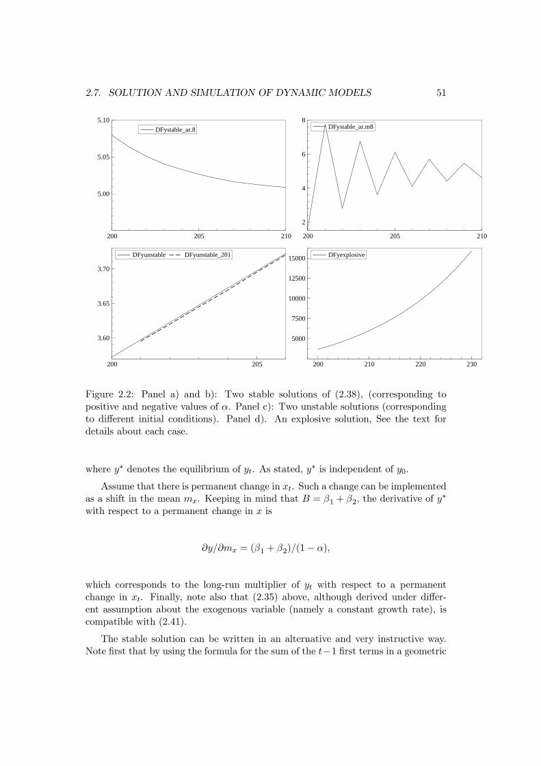
2.7. SOLUTION AND SIMULATION OF DYNAMIC MODELS 51
200 205 210
5.00
5.05
5.10DFystable_ar.8
200 205 210
2
4
6
8DFystable_ar.m8
200 205
3.60
3.65
3.70
DFyunstable DFyunstable_201
200 210 220 230
5000
7500
10000
12500
15000 DFyexplosive
Figure 2.2: Panel a) and b): Two stable solutions of (2.38), (corresponding topositive and negative values of α. Panel c): Two unstable solutions (correspondingto different initial conditions). Panel d). An explosive solution, See the text fordetails about each case.
where y∗ denotes the equilibrium of yt. As stated, y∗ is independent of y0.
Assume that there is permanent change in xt. Such a change can be implementedas a shift in the mean mx. Keeping in mind that B = β1 + β2, the derivative of y
∗
with respect to a permanent change in x is
∂y/∂mx = (β1 + β2)/(1− α),
which corresponds to the long-run multiplier of yt with respect to a permanentchange in xt. Finally, note also that (2.35) above, although derived under differ-ent assumption about the exogenous variable (namely a constant growth rate), iscompatible with (2.41).
The stable solution can be written in an alternative and very instructive way.Note first that by using the formula for the sum of the t−1 first terms in a geometric
52 CHAPTER 2. LINEAR DYNAMIC MODELS
progression,t−1Xs=0
αs can be written as
t−1Xs=0
αs =1− αt
(1− α).
Using this result in (2.39), and next adding and subtracting (β0 +Bmx)αt/(1− α)
on the right hand side of (2.39), we obtain
yt =(β0 +Bmx)
1− α+ αt(y0 −
β0 +Bmx
1− α) (2.42)
= y∗ + αt(y0 − y∗), when − 1 < α < 1.
In the stable case, the dynamic process is essentially correcting the initial discrepancy(disequilibrium) between the initial level of y and its long-run level.
Panel a) of Figure 2.2 shows a numerical example of a stable solution of equation(2.38). In the example we have set α = 0.8 and we have have chosen values of β0and Bmx so that y∗ = 5. We use computer generated data and the initial period(corresponding to t = 0 in the formulae) is t = 200. The initial value is y200 = 5.08.Since the initial value is higher than the equilibrium value, and α is positive, thesolution approaches y∗ = 5 from above.
Panel b) of the figure illustrates another stable solution, namely the solutionfor the case of a negative autoregressive coefficient, α = −0.8. In this case theinitial value is y200 = 1.59, which is markedly lower than the equilibrium of y∗ = 5.According to equation (2.42) the solution for period 201 becomes
y201 = 5− 0.8× (1.59− 5) = 7.73,
and the graph is seen to confirm this. Due to the negative autoregressive coefficientthe solution characteristically oscillates towards the equilibrium value.
2.7.1.2 Unstable solution
When α = 1, we obtain from equation (2.39):
yt = (β0 +Bmx)t+ y0, t = 1, 2, ... (2.43)
showing that the solution contains a linear trend and that the initial condition exertsfull influence over yt even over infinitely long distances. There is of course no welldefined equilibrium where yt settles in the long run, and neither is there a finite long-run multiplier. Nevertheless, the solution is perfectly valid mathematically speaking:given an initial condition, there is one and only one sequence of numbers y1, y2, ...yTwhich satisfy the model.
The instability of the solution is however apparent when we consider not a singlesolution but a sequence of solutions. Assume that we first find a solution conditional
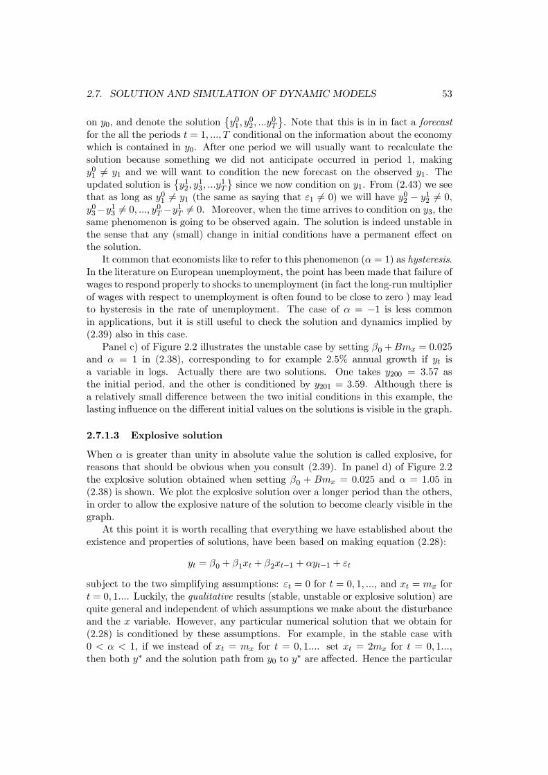
2.7. SOLUTION AND SIMULATION OF DYNAMIC MODELS 53
on y0, and denote the solution©y01, y
02, ...y
0T
ª. Note that this is in in fact a forecast
for the all the periods t = 1, ..., T conditional on the information about the economywhich is contained in y0. After one period we will usually want to recalculate thesolution because something we did not anticipate occurred in period 1, makingy01 6= y1 and we will want to condition the new forecast on the observed y1. Theupdated solution is
©y12, y
13, ...y
1T
ªsince we now condition on y1. From (2.43) we see
that as long as y01 6= y1 (the same as saying that ε1 6= 0) we will have y02 − y12 6= 0,y03−y13 6= 0, ..., y0T −y1T 6= 0. Moreover, when the time arrives to condition on y3, thesame phenomenon is going to be observed again. The solution is indeed unstable inthe sense that any (small) change in initial conditions have a permanent effect onthe solution.
It common that economists like to refer to this phenomenon (α = 1) as hysteresis.In the literature on European unemployment, the point has been made that failure ofwages to respond properly to shocks to unemployment (in fact the long-run multiplierof wages with respect to unemployment is often found to be close to zero ) may leadto hysteresis in the rate of unemployment. The case of α = −1 is less commonin applications, but it is still useful to check the solution and dynamics implied by(2.39) also in this case.
Panel c) of Figure 2.2 illustrates the unstable case by setting β0 +Bmx = 0.025and α = 1 in (2.38), corresponding to for example 2.5% annual growth if yt isa variable in logs. Actually there are two solutions. One takes y200 = 3.57 asthe initial period, and the other is conditioned by y201 = 3.59. Although there isa relatively small difference between the two initial conditions in this example, thelasting influence on the different initial values on the solutions is visible in the graph.
2.7.1.3 Explosive solution
When α is greater than unity in absolute value the solution is called explosive, forreasons that should be obvious when you consult (2.39). In panel d) of Figure 2.2the explosive solution obtained when setting β0 + Bmx = 0.025 and α = 1.05 in(2.38) is shown. We plot the explosive solution over a longer period than the others,in order to allow the explosive nature of the solution to become clearly visible in thegraph.
At this point it is worth recalling that everything we have established about theexistence and properties of solutions, have been based on making equation (2.28):
yt = β0 + β1xt + β2xt−1 + αyt−1 + εt
subject to the two simplifying assumptions: εt = 0 for t = 0, 1, ..., and xt = mx fort = 0, 1.... Luckily, the qualitative results (stable, unstable or explosive solution) arequite general and independent of which assumptions we make about the disturbanceand the x variable. However, any particular numerical solution that we obtain for(2.28) is conditioned by these assumptions. For example, in the stable case with0 < α < 1, if we instead of xt = mx for t = 0, 1.... set xt = 2mx for t = 0, 1...,then both y∗ and the solution path from y0 to y∗ are affected. Hence the particular
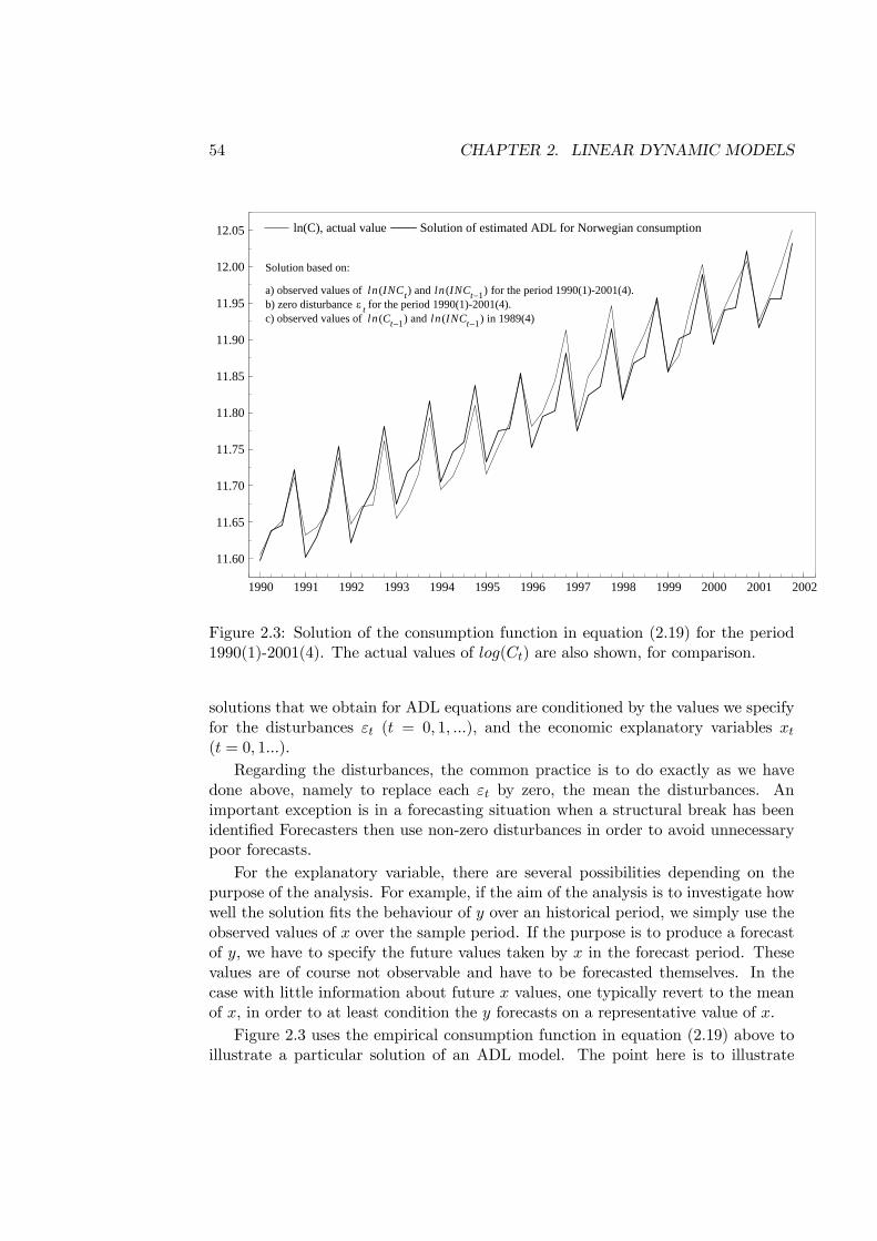
54 CHAPTER 2. LINEAR DYNAMIC MODELS
1990 1991 1992 1993 1994 1995 1996 1997 1998 1999 2000 2001 2002
11.60
11.65
11.70
11.75
11.80
11.85
11.90
11.95
12.00
12.05
Solution based on:
a) observed values of ln (INCt) and ln (INCt−1) for the period 1990(1)-2001(4).b) zero disturbance ε t for the period 1990(1)-2001(4).c) observed values of ln (Ct−1) and ln (INCt−1) in 1989(4)
ln(C), actual value Solution of estimated ADL for Norwegian consumption
Figure 2.3: Solution of the consumption function in equation (2.19) for the period1990(1)-2001(4). The actual values of log(Ct) are also shown, for comparison.
solutions that we obtain for ADL equations are conditioned by the values we specifyfor the disturbances εt (t = 0, 1, ...), and the economic explanatory variables xt(t = 0, 1...).
Regarding the disturbances, the common practice is to do exactly as we havedone above, namely to replace each εt by zero, the mean the disturbances. Animportant exception is in a forecasting situation when a structural break has beenidentified Forecasters then use non-zero disturbances in order to avoid unnecessarypoor forecasts.
For the explanatory variable, there are several possibilities depending on thepurpose of the analysis. For example, if the aim of the analysis is to investigate howwell the solution fits the behaviour of y over an historical period, we simply use theobserved values of x over the sample period. If the purpose is to produce a forecastof y, we have to specify the future values taken by x in the forecast period. Thesevalues are of course not observable and have to be forecasted themselves. In thecase with little information about future x values, one typically revert to the meanof x, in order to at least condition the y forecasts on a representative value of x.
Figure 2.3 uses the empirical consumption function in equation (2.19) above toillustrate a particular solution of an ADL model. The point here is to illustrate
2.7. SOLUTION AND SIMULATION OF DYNAMIC MODELS 55
how well the solution fits the actual data over the sample period, so the solution isconditioned by the actual observations for income. The figure shows the solution for(the logarithm) of consumption over the period 1989(1)-2001(4) together with theobserved actual values of consumption over that period. The scale of the vertical axisindicates that real private consumption expenditure has increased by a formidable50% over the period, and the graph shows that this development is well explainedby the solution of the consumption function. That the solution is conditioned by thetrue values of income, must be taken into account when assessing the close captureof the trend-growth in consumption.
Also apparent from the graph is a marked seasonal pattern: consumption ishighest in the 3rd and 4th quarter of each year. Seasonality is a feature of manyquarterly or monthly time series. How to represent seasonality in a model is questionin its own right and cannot be answered in any detail within the scope of this book.However the interested reader might note that in order to capture seasonality aswell as we do in the figure, we have included so called seasonal dummies, but forsimplicity, the estimated coefficient have been suppressed in equation (2.19).13
2.7.2 Simulation of dynamic models
In applied macroeconomics it is not always common to refer to the solution of adynamic model. The customary term is instead simulation. Specifically, economistsuse dynamic simulation to denote the case where the solution for period 1 is usedto calculate the solution for period 2, and the solution for period 2 is in turn usedto find the solution for period 3, and so on. In the case of a single ADL equationwith one lag, which we have studied extensively above, dynamic simulation clearlyamounts to finding the solution of that model. Conveniently, the correspondencebetween solution and dynamic simulation also holds for equations with several lagsand/or several explanatory variables, as well as for the systems of dynamic equationsthat are used in macroeconomic practice. The dominance of simulation stems fromthe fact that simulation offers an easy way of finding the solution in the cases wherethe closed form algebraic solution is impractical.
Reflecting the practical usefulness of simulation in macroeconomics is the factthat modern econometric software packages contain a wide range of built-in pos-sibilities for simulation analysis, as well as rich possibilities for reporting of thesimulation results, in numerical or in graphical form. Depending on the purpose ofthe simulation, it is custom to distinguish between three main types of simulationanalyses. These are: track-analysis, forecasting, and multiplier analysis.
When we do track-analysis, simulation is used to find how fell the solution of anestimated macroeconomic model tracks the actual values of the endogenous variablesover the sample period) and figure 2.3 provides an example. Dynamic simulationis also the practical way produce forecasts from dynamic models. However, a main
13Seasonal dummies are explained in any introductory textbook in econometrics. To reproducethe detailed results underlying Figure 2.3, consult the file norcons.zip on the web page.
56 CHAPTER 2. LINEAR DYNAMIC MODELS
complication that distinguishes a historical dynamic simulation from a dynamic fore-cast is that, since observations of the x variable are only available for the historicalsample period (t = 1, 2, ...T ) they also need to be forecasted before we can simulateyt for a H periods ahead. H is often referred to as the forecast horizon. Havingfixed a set of values xT+1, xT+2, ...,xT+H , the simulated values yT+1, yT+1, ..., yT+H ,correspond to the solution based on the initial values xT , xT−1. and yT−1.
When forecasting, the determination of the future sequence x are is not at all atrivial matter. Sometimes, the forecaster characterizes the sequence of x values asrepresenting a possible future, not necessarily the most likely future realizations ofx’s. In this case, the forecast is usually referred to as a scenario of the future, and theforecaster often choose to illustrate two or more scenarios for the forecasted variabley, corresponding to for example “high” and “low” future realizations of x. The othermain motivation for a forecasts is to obtain the most likely future development ofyT+j and xT+j , given the information available in period T . In this case, the equationfor yt has to be supplemented with an equation for xt, and the dynamic simulationof that 2-equation model based on yT and xT (and knowledge of the parameters)represent the forecast. Such forecasts are called conditional forecasts, because theyare conditioned by the history of the system consisting of the equations for yt and xtup to period T . Another much used term is that the conditional forecast correspondto rational expectations.
Finally, dynamic simulation is used to produce dynamic multipliers. In thatcase we do two dynamic simulations: first, a baseline simulation using a baseline orreference set of values of the x variable (often these are the historical values, or abaseline forecast), and second, an alternative simulation based on an alternative (or“shocked”) set of x values. As always, the initial condition has to be specified beforethe solution can be found. Since the focus is on the effect of a change in x, the sameinitial condition is used for both the baseline and the alternative simulation. If wedenote the baseline solution ybt and the alternative y
at , the difference y
at − ybt are the
dynamic multipliers.
We end this section by noting that care must be taken to distinguish betweenstatic simulation, which is also part of the vocabulary used by macroeconomists,and dynamic simulation which we have discussed so far. In a static simulation, theactual (not the simulated) values for y in period t− 1 is used to calculate yt. Thusthe sequence of y’s obtained from a static simulation does not correspond to thesolution of the ADL model. Static and dynamic simulations give an identical resultonly for the first period of the simulation period. Since, in practice, we use estimatedvalues of the model’s coefficient when we simulate a model, the resulting y−valuesfrom a static simulation over the sample period are identical to the equation’s fittedvalues.14
14Strictly speaking, this is only true for single equation models. If we consider a system ofsimultaneous equations, the fitted values of a single endogenous variable are different form thesolved out values from a static simulation.
2.8. DYNAMIC SYSTEMS 57
2.8 Dynamic systems
In macroeconomics, the effect of a shock or policy change is usually dependent onsystem properties. As a rule it is not enough to consider only one equation in orderto obtain the correct dynamic multipliers. Consider for example the consumptionfunction of section 2.2 where it was assumed that income (INC) was an exogenousvariable. This exogeneity assumption is only tenable given some further assumptionsabout the rest of the economy: for example if there is a general equilibrium withflexible prices and the supply of labour is fixed, then output and income may beregarded as independent of Ct. However, with sticky prices and idle resources, i.e.,the Keynesian case, INC must be treated as logically be considered as an endogenousvariable. Generally, because the different sectors and markets of an economy areinterlinked, the limitations of the single equation analysis we have considered so farin this chapter is rather obvious.
Nevertheless, the discussion if the solution of a single ADL equation providesessential background for understanding dynamic models, so our efforts so far arenot wasted. First, it is often quite easy to bring a system on a form with tworeduced form dynamic equations that are of the same form that we have consideredabove. After this step, we can derive the full solution of each endogenous variableof the system if we so want. Section 2.8.1, 2.8.3 and 2.8.4 show specific examples.Second, in more complicated cases where a full analysis of the system is beyond us(at least without the aid of computer simulation), it is still relatively easy to findthe short-run and long-run multipliers of the endogenous variables with respect tochanges in the exogenous variables, by drawing on the distinction between the short-run and long-run version of the models that we introduced in chapter 1.4, and whichwe re-state in section 2.8.2 below. Third, as already hinted, computer simulationrepresents a practical way of obtaining the solution of systems of dynamic equationswith quantified coefficient values and known initial conditions, for i.e., the systemsof equations used in practice for forecasting and policy analysis, and the conceptsthat we have introduced above are essential in the interpretation of the results fromsuch computer based simulation.
2.8.1 A dynamic income-expenditure model
We begin by showing how the analysis of the dynamic consumption function with ischanged when the assumption of exogenous income is replaced by an assumption ofendogenous income. For this purpose it is most practical to specify a consumptionfunction which is linear in variables, rather than being linear only in parameters aswe have used frequently above. Hence, the model is made up of a linear consumptionfunction
Ct = β0 + β1INCt + αCt−1 + εt, (2.44)
and a product market equilibrium condition
INCt = Ct + Jt, (2.45)
58 CHAPTER 2. LINEAR DYNAMIC MODELS
where Jt denotes autonomous expenditure, and where INC is now interpreted as thegross domestic product, GDP. We assume that there are idle resources (unemploy-ment) and that prices are sticky, so that income is determined “from the demandside”. The 2-equation dynamic system has two endogenous variables Ct and INCt,while Jt and εt are exogenous.
To find the solution for consumption, substitute INC from (2.45), and obtain
Ct = β0 + αCt−1 + β2Jt + εt (2.46)
where β0 and α are the original coefficients divided by (1−β1), and β2 = β1/(1−β1),and εt = εt/(1− β1).
Equation (2.46) is yet another example of an ADL model, so the theory of theprevious sections applies. For a given initial condition C0 and known values for thetwo exogenous variables (e.g., {J1, J2, ..., JT}) there is a unique solution. If −1 <α < 1 the solution is asymptotically stable. The impact multiplier of consumptionwith respect to autonomous expenditure is β2, while in the stable case, the long-runmultiplier is β2/(1− α). If the system (2.44) and (2.45) implies a stable solution forCt, there is obviously also a stable solution for INCt, meaning that we do not haveto derive the solution for INCt in order to check the dynamic stability of income.
Equation (2.46) is called the final equation for Ct. The defining characteristic ofa final equation is that (apart from exogenous variables) the right hand side onlycontains lagged values of the left hand side variable. It is often feasible to derive afinal equation for more complex systems than the one we have studied here. Theconditions for stability of the system as a whole (i.e., all the endogenous variables areasymptotically stable) is then expressed in terms of the so called characteristic rootsof the final equation. The relationship between α1, α2 and the characteristic roots ofthe final equation goes beyond the scope of this course, but it can be mentioned thata sufficient condition for stability of a final equation with second order dynamics (i.e.,not only yt−1 but also yt−2 is part of the equation for yt) is that both α1 and α2 areless than one. Section 2.8.5 below states these points in a more general framework.
2.8.2 The method with a short-run and long-run model
It is worth reminding ourselves about the analysis of dynamic models that was in-troduced in chapter 1.4. When we are working with models with more than twoendogenous variables, or with two or more lags, we are often unable to derive thefull solution of the dynamic model, at least without the aid of the mathematicalalgorithms provided by relevant computer programmes. However, by using the sim-plified step-wise approach, we can still answer two important questions: i) Whatare the short-run effect of a change in an exogenous variable, and ii) what are thelong-run effects of the shocks. The method, as we saw in chapter 1.4, amounted tousing two versions of the model: a short-run version, and a long-run version of themodel.
In the income-expenditure model the short-run model is given by (2.44) and(2.45), where Ct and INCt are endogenous variables, Ct−1 is a predetermined ex-
2.8. DYNAMIC SYSTEMS 59
ogenous variable, and Jt and εt are exogenous variables. The long-run model isdefined for the situation of Ct = C, INCt = INC, Jt = J and εt = 0, and is writtenas
C =β01− α
+β11− α
INC (2.47)
INC = C + J (2.48)
In exactly the same manner as in chapter 1.4, the impact multiplier of a permanent(or temporary) rise in Jt is obtained from the short-run model (2.44) and (2.45),while subject to dynamic stability, the long-run multipliers can be derived from thestatic system method (2.47)-(2.48). It is a useful exercise to check that the long-runmultipliers from the long-run model are the same as the ones you obtained from thefinal equations of Ct and INCt.
2.8.3 The basic Solow growth model
Growth theory is often the economics student’s first encounter with a dynamicmodel, and here we only briefly review the simplest Solow growth model usingthe framework developed above.15 The first equation of the model is the macroproduction function of the Cobb-Douglas type,
Yt = Kγt Nt
1−γ , 0 < γ < 1 (2.49)
where Yt is GDP in period t, Kt denotes the capital stock, and Nt is employment inperiod t. In the basic version of them model we simply define Nt as the number ofemployed persons, which in turn is identical to the size the population. Hence fullemployment is assumed, and we abstract from variations in working time. The sizeof the population is assumed to grow with a constant rate n:
Nt
Nt−1− 1 = n, n ≥ 0 (2.50)
We have to be precise about the dating of the capital stock, since the third equationof the model links the evolution of the capital stock to the flow of investment. Inaccordance, with section (1.6) above, we define Kt as the amount of capital availableat the start of period t. We next assume that all saving, St, in period t is investedso that the “law of motion” for the capital stock is
Kt = (1− δ)Kt−1 + St−1, 0 < δ ≤ 1 (2.51)
where δ is the rate of depreciation of capital, consistent with (1.13) in chapter 1. Inthe Solow model, an essential assumption is that saving is proportional to income,hence15A good reference to both the basic version of the Solow model, and to the different extensions of
the model with e.g., technological progress is the textbook by Birch Sørensen and Whitta-Jacobsen(2005). The basic Solow model is for example presented in Birch Sørensen and Whitta-Jacobsen(2005, Chapter 3.2).
60 CHAPTER 2. LINEAR DYNAMIC MODELS
St = sYt, 0 ≤ s < 1 (2.52)
where s is the fraction saved out of income in each period.Let us first see what the steady state solution of this dynamic model looks like,
assuming that a unique and stable steady state solution exists. To formulate thelong-run mode /l, we first note that if we want to write the model in terms of variablesthat are independent of time in steady state, we cannot use Y , N and K directlysince population is growing with rate n in steady state, by assumption. Instead, letus make the initial guess that capital intensity kt = Kt/Nt is a variable that is aconstant k in steady state. If this is true, the long-run model, i.e., the model for thesteady state takes the form
y =¡k¢γ (2.53)
k =1
(δ + n)s · y (2.54)
where GDP per capital is denoted y = Y/N , and y is the steady state value of GDPper capita. If (2.53) and (2.54) characterizes the steady state, we can combine thetwo equations to obtain the following equation for y
y =
∙1
(δ + n)s · y
¸γ(2.55)
which shows that a permanent increase in the saving rate s has the following long-runeffect on GDP per capita:
d ln y
d ln s=
γ
1− γ> 0, (2.56)
or, in derivative form:dy
ds=
y
s
γ
1− γ(2.57)
which says that a permanent increase in the saving rate has a positive long run effecton GDP per capita, and that the effect is larger the larger y is in the initial steadystate situation.
Next, we address the more demanding task of checking whether the long-runmodel made up of (2.53) and (2.54) does indeed represent a stable steady statesolution of the Solow model (2.49)-(2.52). For that purpose we need to derive thefinal equation for the dynamic system. We start with equation (2.51) and divide onboth sides by Nt−1:
Kt
Nt−1= (1− δ)
Kt−1Nt−1
+St−1Nt−1
.
On the left-and side, multiply by Nt/Nt, and use (2.50) and (2.52) to obtain:
kt(1 + n) = (1− δ)kt−1 + s yt−1 (2.58)
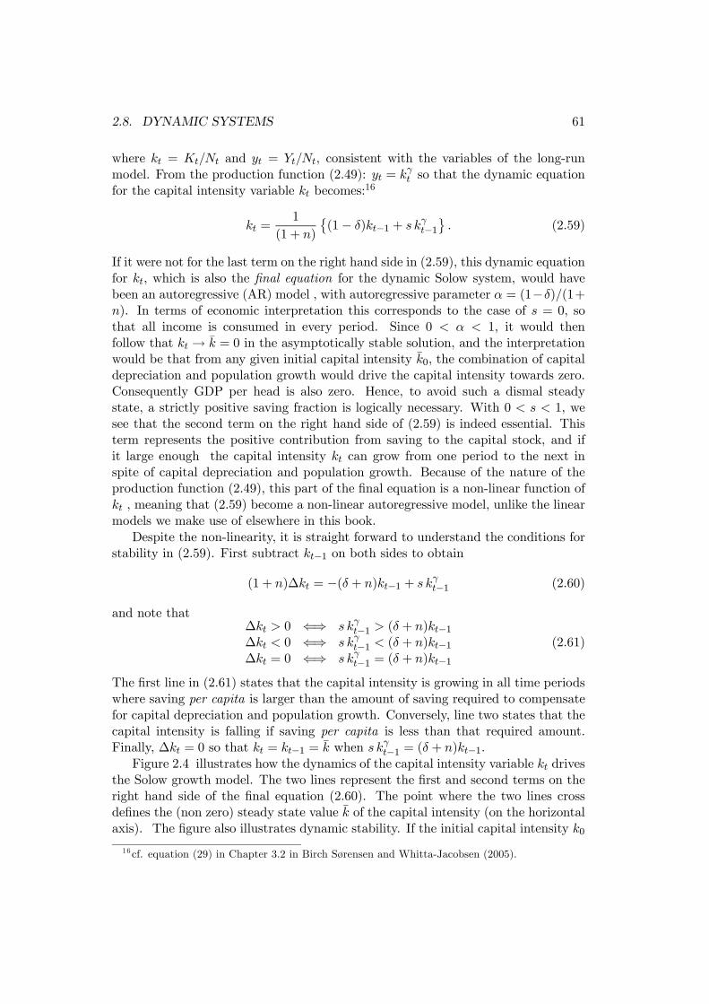
2.8. DYNAMIC SYSTEMS 61
where kt = Kt/Nt and yt = Yt/Nt, consistent with the variables of the long-runmodel. From the production function (2.49): yt = kγt so that the dynamic equationfor the capital intensity variable kt becomes:16
kt =1
(1 + n)
©(1− δ)kt−1 + s kγt−1
ª. (2.59)
If it were not for the last term on the right hand side in (2.59), this dynamic equationfor kt, which is also the final equation for the dynamic Solow system, would havebeen an autoregressive (AR) model , with autoregressive parameter α = (1−δ)/(1+n). In terms of economic interpretation this corresponds to the case of s = 0, sothat all income is consumed in every period. Since 0 < α < 1, it would thenfollow that kt → k = 0 in the asymptotically stable solution, and the interpretationwould be that from any given initial capital intensity k0, the combination of capitaldepreciation and population growth would drive the capital intensity towards zero.Consequently GDP per head is also zero. Hence, to avoid such a dismal steadystate, a strictly positive saving fraction is logically necessary. With 0 < s < 1, wesee that the second term on the right hand side of (2.59) is indeed essential. Thisterm represents the positive contribution from saving to the capital stock, and ifit large enough the capital intensity kt can grow from one period to the next inspite of capital depreciation and population growth. Because of the nature of theproduction function (2.49), this part of the final equation is a non-linear function ofkt , meaning that (2.59) become a non-linear autoregressive model, unlike the linearmodels we make use of elsewhere in this book.
Despite the non-linearity, it is straight forward to understand the conditions forstability in (2.59). First subtract kt−1 on both sides to obtain
(1 + n)∆kt = −(δ + n)kt−1 + s kγt−1 (2.60)
and note that∆kt > 0 ⇐⇒ s kγt−1 > (δ + n)kt−1∆kt < 0 ⇐⇒ s kγt−1 < (δ + n)kt−1∆kt = 0 ⇐⇒ s kγt−1 = (δ + n)kt−1
(2.61)
The first line in (2.61) states that the capital intensity is growing in all time periodswhere saving per capita is larger than the amount of saving required to compensatefor capital depreciation and population growth. Conversely, line two states that thecapital intensity is falling if saving per capita is less than that required amount.Finally, ∆kt = 0 so that kt = kt−1 = k when s kγt−1 = (δ + n)kt−1.
Figure 2.4 illustrates how the dynamics of the capital intensity variable kt drivesthe Solow growth model. The two lines represent the first and second terms on theright hand side of the final equation (2.60). The point where the two lines crossdefines the (non zero) steady state value k of the capital intensity (on the horizontalaxis). The figure also illustrates dynamic stability. If the initial capital intensity k016 cf. equation (29) in Chapter 3.2 in Birch Sørensen and Whitta-Jacobsen (2005).
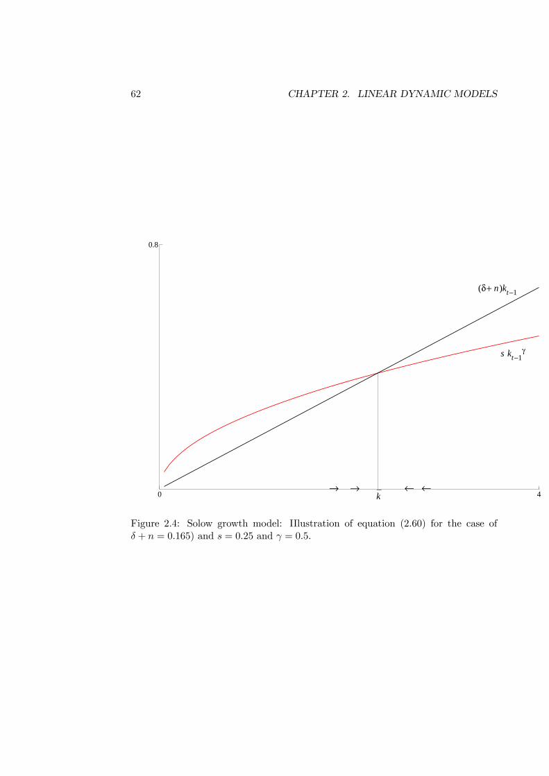
62 CHAPTER 2. LINEAR DYNAMIC MODELS
0 4
0.8
(δ+ n)kt−1
s kt−1γ
k→→ ← ←
Figure 2.4: Solow growth model: IIlustration of equation (2.60) for the case ofδ + n = 0.165) and s = 0.25 and γ = 0.5.
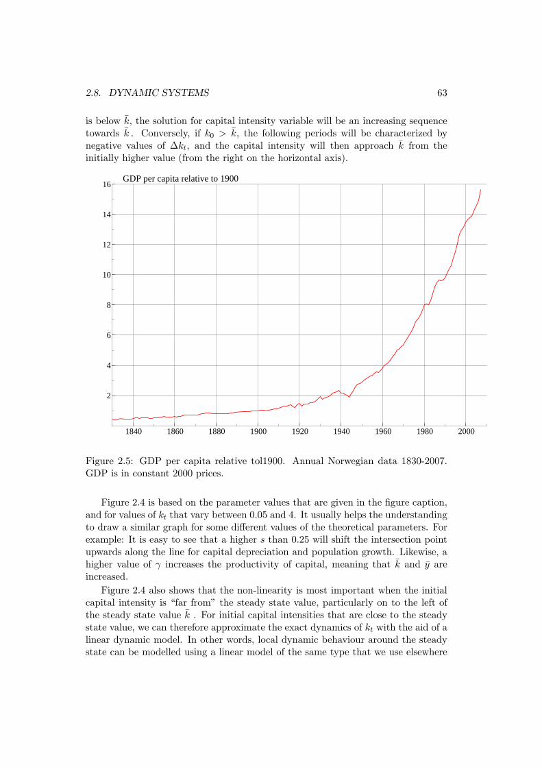
2.8. DYNAMIC SYSTEMS 63
is below k, the solution for capital intensity variable will be an increasing sequencetowards k . Conversely, if k0 > k, the following periods will be characterized bynegative values of ∆kt, and the capital intensity will then approach k from theinitially higher value (from the right on the horizontal axis).
1840 1860 1880 1900 1920 1940 1960 1980 2000
2
4
6
8
10
12
14
16GDP per capita relative to 1900
Figure 2.5: GDP per capita relative tol1900. Annual Norwegian data 1830-2007.GDP is in constant 2000 prices.
Figure 2.4 is based on the parameter values that are given in the figure caption,and for values of kt that vary between 0.05 and 4. It usually helps the understandingto draw a similar graph for some different values of the theoretical parameters. Forexample: It is easy to see that a higher s than 0.25 will shift the intersection pointupwards along the line for capital depreciation and population growth. Likewise, ahigher value of γ increases the productivity of capital, meaning that k and y areincreased.
Figure 2.4 also shows that the non-linearity is most important when the initialcapital intensity is “far from” the steady state value, particularly on to the left ofthe steady state value k . For initial capital intensities that are close to the steadystate value, we can therefore approximate the exact dynamics of kt with the aid of alinear dynamic model. In other words, local dynamic behaviour around the steadystate can be modelled using a linear model of the same type that we use elsewhere
64 CHAPTER 2. LINEAR DYNAMIC MODELS
in the book. To illustrate this point, using the principles of linearization, a so calledfirst order approximation to (2.59) becomes
kt ≈µ1− δ
1 + n+
s
1 + nγkγ−1
¶kt−1 + s
1− γ
1 + nkγ (2.62)
which is an AR equation.17 Assuming that the autoregressive coefficient is between0 and 1 (2.62) is consistent with dynamic stability in the neighborhood of the steadystate capital intensity k.
Solow’s growth model is the standard model for economic analysis with a timehorizon that goes beyond the length of the typical business-cycle of 5-10 years. Inorder to be able to explain the facts of economic growth the basic model that wehave presented here obviously needs to be replaced by a model that incudes moregrowth explaining factors. As one example, Figure 2.5 shows that GDP per capita inNorway has grown by a factor of 16 since 1900, while the basic Solow model indicateszero growth in steady state. However, we leave it to a course in economic growththeory to show that inclusion of technological progress is one of the modificationsthat help reconcile the theory’s predictions with growth statistics. Instead, we turnto a model that applies the Solow model’s framework to a much shorter time horizonthan was originally intended.
2.8.4 A real business cycle model
The real business cycle (RBC) approach applies the framework of the Solow modelthe business cycle. So unlike the Solow model, where the time period t typicallyrefers to a 5 or 10 years averages, the time period t in the RBC refers to years orquarters of a year.
The Keynesian income-expenditure model and the RBC model are regarded acontesting explanations of short-run macroeconomic fluctuations. This is because ofthe differences in assumptions, in particularly regarding the labour market and un-employment. In the Keynesian model, there is involuntary unemployment, the realwage does not correspond to the market clearing real wage of a perfectly competitivelabour market, and the business cycle is regarded as disequilibrium phenomenon. Inthe RBC model, there is no genuine involuntary unemployment. Instead, recordedunemployment is regarded as a misnomer for intertemporal substitution of workingtime for leisure, and the business cycle is an equilibrium phenomenon.
The first equation of the RBC model is the macro production function (2.49),augmented by a technology variable At
Yt = Kγt (AtNt)
1−γ , 0 < γ < 1, (2.63)
and where we, because of the change of time horizon and the change in focus tobusiness-cycle fluctuations, change the interpretation of Nt from persons employedto the total number of hours worked, i.e., the number of workers times the average17Appendix B gives the details.
2.8. DYNAMIC SYSTEMS 65
length of the working day. This specification of the production function is referredto as labour augmenting technical progress, since an increase in At implies thatGDP is increased without any increase in the capital stock (labour becomes moreproductive).18 It is important in the following that technical progress is modelled asthe sum of two parts: one completely deterministic part and a second part which israndom. The deterministic part is a given rate of technological progress gA multi-plied by time, which we write gAt, and the random part is denoted as,t. Hence, theRBC model’s theory of technological progress is given by
lnAt = gAt+ as,t, 0 < gA < 1, (2.64)
where the random part is given by the autoregressive equation:
as,t = αas,t−1 + εa,t, 0 ≤ α < 1 (2.65)
where εa,t is a completely unpredictable technology shock. We can amalgamate thetwo technology equations into one by lagging (2.64) one period, and then multiplyingby α on both sides of the lagged equation:
α lnAt−1 = αgA(t− 1) + αas,t−1. (2.66)
Subtraction of equation (2.66) from (2.64) gives
lnAt = αgA + gA(1− α)t+ α lnAt−1 + εa,t, (2.67)
which shows that technological progress lnAt is implied to follow an autoregressivemodel augmented by a deterministic trend αgA(t− 1). We can re-write (2.67) as
lnAt − lnAt−1 = αgA + gA(1− α)t+ (α− 1) lnAt−1 + εa,t, (2.68)
and define a steady state as a situation where all shocks are zero, i.e., εa,t = 0 forall t. Let ln At denote steady state productivity. From (2.67) with εa,t = 0, we notethat ln At−1 is given by
gA = αgA + gA(1− α)t+ (α− 1) ln At−1
orln At−1 = −gA + gAt.
since ln At = gA + ln At−1 we have
ln At = gAt (2.69)
showing that (2.64) can alternatively be written as
lnAt = ln At + as,t, (2.70)
18We adopt more or less the same assumptions as in the expositition in Birch Sørensen andWhitta-Jacobsen (2005, Chapter 19.4).
66 CHAPTER 2. LINEAR DYNAMIC MODELS
as long as the restriction on gA is observed.The RBC model makes uses also of the saving equation (2.52), and the capital
evolution equation (2.51), which we however simplify by setting δ = 1, meaning thatcapital equipment lasts for only one period, so that
Kt = St−1. (2.71)
It is the infallible mark of RBC models that the labour market is assumed to bein equilibrium in each period. Labour supply, NS
t , is a function of the relative wagewt/wt:
NSt = N(
wt
wt) , > 0. (2.72)
where wt is the steady state wage and is the labour supply elasticity. Whenthe wage is equal to the steady state wage, labour supply is also equal to its steadystate value. Though simple in appearance, equation (2.72) is representing optimizingbehaviour by households and individuals: They choose to supply labour in excess ofthe long-run level determined by demography and sociological norms and legislaturewhen the real wage wt is higher than the steady state real wage wt, and to substitutelabour for leisure in times when the real wage is low relative its long run level. Forsimplicity of exposition we set N = 1 in the following, since in (2.72) this is merelya choice of units.
Labour demand is obtained by assuming optimizing behaviour by a ‘macro pro-ducer’, and the marginal product of labour is therefore set equal to the real wage:
wt = (1− γ)
µKt
AtNt
¶γ
At = (1− γ)
µYtNt
¶. (2.73)
The assumption of equilibrium in the labour market means that NSt = Nt, and we
can solve (2.72) and (2.73) for real wage and for employment. First, note that from(2.72):
wt = N1
t wt (2.74)
Next, note that the ratioKt/AtNt in (2.73) is a generalization of the capital intensityvariable kt of the Solow model. The generalization is due to the inclusion of theproductivity At variable in the RBC production function, hence we define kA,t =Kt/AtNt as the productivity corrected capital intensity. Moreover, with referenceto the Solow model above, we define kA as the steady state value of the productivitycorrected capital intensity. The corresponding steady state real wage, from (2.73),is
wt = (1− γ)kγAAt. (2.75)
Remember that both wt and kA refer to the situation with εa,t = 0 (there are noshocks in the steady state). Using (2.74) and (2.75) we obtain
wt = N1
t (1− γ)kγAAt. (2.76)
2.8. DYNAMIC SYSTEMS 67
A this point we take the natural logarithms on both sides of (2.73), and (2.76):
lnwt = ln(1− γ) + lnYt − lnNt,
lnwt =1lnNt + ln((1− γ)kγAAt).
Using these two expressions to solve for lnNt gives
lnNt =1 +
©lnYt − ln(kγAAt)
ª. (2.77)
Substitution of the this expression together with (2.71) and (2.52) into the log ofthe production function, (2.63), gives
lnYt = γ ln(sYt−1) + (1− γ)
µ1 +
©lnYt − ln(kγAAt)
ª¶+ (1− γ) lnAt
1 + γ
1 +lnYt = γ ln s+ γ ln(Yt.−1) + (1− γ)
µ−1 +
ln(kγAAt)
¶+ (1− γ) lnAt
and eventually
lnYt =γ(1 + )
1 + γln s+
γ(1 + )
1 + γlnYt−1 −
(1− γ)
1 + γln(kγAAt) +
(1− γ)(1 + )
1 + γlnAt.
(2.78)Note that this is the final equation for lnYt in the RBC model: it expresses lnYt byits lag and by exogenous variables. Noting that ln At and lnAt are linked throughequation (2.70) above, and that ln At = gAt in (2.69) above, the final equation forlnYt can be written as
lnYt =γ(1 + )
1 + γln s−(1− γ)
1 + γln(kγA)+
γ(1 + )
1 + γlnYt−1+
(1− γ)
1 + γgAt+
(1− γ)(1 + )
1 + γas,t
(2.79)where as,t follows the autoregressive process in equation (2.65) above.
There are several important notes to be made about (2.79). First, dynamicstability hinges on the autoregressive parameter being less than one in magnitude.We see that in (2.79) the stability condition is satisfied, since
γ(1 + )
1 + γ=
γ(1 + ) + 1− 11 + γ
= 1− 1− γ
1 + γ
is a number between 0 and 1, based the assumptions of the model. Second, givenstability, there is a deterministic steady state growth path for Yt with growth rategA. Third, and heuristically speaking, the only difference between (2.79) and theimplied equation for the log of the steady state GDP, ln Yt, is that the equation forln Yt does not contain the stochastic technology shock term.19 Hence, the equationfor ln Yt is:
ln Yt =γ(1 + )
1 + γln s− (1− γ)
1 + γln(kγA) +
γ(1 + )
1 + γln Yt−1 +
(1− γ)
1 + γgAt, (2.80)
19This can be made precice by taking the mathematical expectation of (2.79).
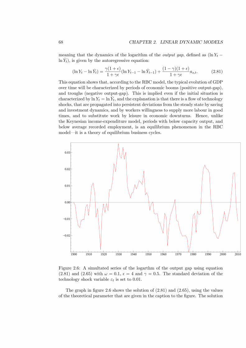
68 CHAPTER 2. LINEAR DYNAMIC MODELS
meaning that the dynamics of the logarithm of the output gap, defined as (lnYt −ln Yt), is given by the autoregressive equation:
(lnYt − ln Yt) =γ(1 + )
1 + γ(lnYt−1 − ln Yt−1) +
(1− γ)(1 + )
1 + γas,t. (2.81)
This equation shows that, according to the RBC model, the typical evolution of GDPover time will be characterized by periods of economic booms (positive output-gap),and troughs (negative output-gap). This is implied even if the initial situation ischaracterized by lnYt = ln Yt, and the explanation is that there is a flow of technologyshocks, that are propagated into persistent deviations from the steady state by savingand investment dynamics, and by workers willingness to supply more labour in goodtimes, and to substitute work by leisure in economic downturns. Hence, unlikethe Keynesian income-expenditure model, periods with below capacity output, andbelow average recorded employment, is an equilibrium phenomenon in the RBCmodel–it is a theory of equilibrium business cycles.
1900 1910 1920 1930 1940 1950 1960 1970 1980 1990 2000 2010
−0.02
−0.01
0.00
0.01
0.02
0.03
Figure 2.6: A simultated series of the logarthm of the output gap using equation(2.81) and (2.65) with ω = 0.1, = 4 and γ = 0.5. The standard deviation of thetechnology shock variable εt is set to 0.01.
The graph in figure 2.6 shows the solution of (2.81) and (2.65), using the valuesof the theoretical parameter that are given in the caption to the figure. The solution
2.8. DYNAMIC SYSTEMS 69
assumes that the output-gap is zero in the initial year, which we have set to “1900”in the simulation and in the graph. Due to negative productivity shocks in the firstyears of the solution period, and propagation, the output-gap is negative for thefirst 10 years, before there is a brief upturn after 12-13 years. The first more lastingboom starts in the mid “1920’s” and lasts for more than 25 years. It is followed bya long period of GDP below steady state. At the end of the solution period, thedistance between the waves of high income generation is shorter again.
It gives rise to thought that a simple RBC model can generate economic upturnsand downturn that are of so long duration as shown in figure 2.6. One lessonmay be that one should not jump to conclusions about economic disequilibria orunbalances in the economy on the basis of 10 years of above or below trend economicperformance–further analysis is required to determine whether the business cycleis a equilibrium or disequilibrium phenomenon.
2.8.5 The solution of the bivariate first order system (VAR)
The income-expenditure model contain first order dynamics because of the laggedterm in the consumption function. More generally, if we consider two equations inthe two variables xt and yt, both xt−1 and yt−1 appear in each of the equations:
yt = α11yt−1 + α12xt−1 + εyt, (2.82)
xt = α21yt−1 + α22xt−1 + εxt. (2.83)
where αij are constant coefficients, and εyt, εxt are two random variables, both withmean zero.
The two equations (2.82) and (2.83) define what is known in the literature as avector autoregressive model, or VAR. The reason for this name is that if we definethe vectors zt = (yt, xt)0, and εt = (εyt, εxt)0, and a matrix
α =
µα11 α12α21 α22
¶,
the vector zt is seen to follow a first order autoregressive model:
zt = α zt−1 + εt. (2.84)
Often in economics, the VAR needs to be extended by exogenous explanatory vari-ables, Hence if we let wt represent an explanatory variable with mean, mw 6= 0, anddefine the coefficient vector β = (β10, β20), the vector autoregressive distributed lagmodel (often called VAR-X) is given by
yt = α11yt−1 + α12xt−1 + β10wt + εyt, (2.85)
xt = α21yt−1 + α22xt−1 + β20wt + εxt. (2.86)
orzt = α zt−1 + βwt + εt. (2.87)
70 CHAPTER 2. LINEAR DYNAMIC MODELS
in matrix notation.The short-run model in this case is clearly given by (2.85) and (2.86)–or by
(2.87) if matrices are used.. The impact multipliers are given by the vector β. If astable solution exists, the long-run model is given by
y = α11y + α12x+ β10mw, (2.88)
x = α21y + α22x+ β20mw. (2.89)
where y and x denote the two steady state values of the endogenous variables.By solving the two simultaneous equations (2.88) and (2.89) we find the long-runsolution as
y =(α22 − 1)β10 − α12β20
α11 + α22 − α11α22 + α12α21 − 1mw, (2.90)
x =−α21β20 + (α11 − 1)β10
α11 + α22 − α11α22 + α12α21 − 1mw. (2.91)
The long-run multipliers are the derivatives of (2.90) and (2.91).A full discussions of the stability conditions for the bivariate first order system
goes beyond the scope of this course. But it is possible to gain important insightby deriving the final equation for yt. From the single equation case, we know thatstability hinges on the autoregressive part of the model, not on the distributed lagpart. The same is true here: what matters is the dynamic interdependence betweenthe two endogenous variables. Hence, to save notation, and we can find the finalequation for the case of β10 = β20 = 0 and εyt, = εxt = 0. First note that (2.82) and(2.83) also holds for period t− 1.
yt−1 = α11yt−2 + α12xt−2
xt−1 = α21yt−2 + β21xt−2.
From the first equation obtain
xt−2 =−1α12
(α11yt−2 − yt−1),
and substitute this for xt−2 in the second equation to obtain.
xt−1 = α21yt−2 −α22α11α12
yt−2 +α22α12
yt−1.
The left hand side of this equation can be substituted for xt−1 in equation (2.82) togive the final equation for yt:
yt = (α11 + α22)yt−1 + (α12α21 − α11α22)yt−2. (2.92)
Since this is an autoregressive equation with two lags it is immediately clear thatfor example a11 < 1 by itself does not guarantee the existence of a stable solution.
2.8. DYNAMIC SYSTEMS 71
Conversely, it is possible that the system is dynamically stable even when for exampleα11 = 1, i.e., if the other coefficients “contributes enough to stability”. The necessaryand sufficient conditions for stability can be shown to be (see Sydsæter and Berck(2006, p 66, equation 10.18)):
1− (α12α21 − α11α22) > 0
1− (α11 + α22) + (α12α21 − α11α22) > 0
1 + (α11 + α22) + (α12α21 − α11α22) > 0.
Inspection of these conditions show that they are in terms of the coefficients of thefinal equation (2.92). As hinted above, the conditions for stability are seen to befulfilled if both those coefficients are less than one.
Exercises
1. Use Table 2.1 to check the multipliers reported in Table 2.2.
2. Show that, after setting et = 0 (for convenience), MPC ≡ ∂Ct/∂INCt =
k · β1INCβ1−1t , where k = exp(β0).
3. Confirm that in the case of a distributed lag model, the two first multipliers ofa temporary change are equal the coefficients of xt and xt−1 respectively, whileδj = 0 for j = 2, 3,. . . . Show also that in the case of a permanent change,δlong−run is equal to β1 + β2.
4. Using the definitions of dynamics, in what sense would you say that the Dif-ferenced data model of section 2.3 qualifies as a dynamic model, and in whichsense does it (rather) qualify as a static model?
5. In a dynamic system with two endogenous variables, explain why we only needto derive one final equation in order to check the stability of the system.
6. In the model in section 2.8, derive the final equation for INCt. What is therelationship between the demand multipliers that you know from Keynesianmodels, and the impact and long-run multipliers of INC with respect to a oneunit change in autonomous expenditure?
7. Formulate a dynamic model of the nominal exchange rate which is consistentwith the PPP hypothesis holding as a long-run proposition.
8. Let σt denote the real exchange rate period t. Assume that the time period isannual, and that we are given the following ADL model which explains σt:
σt = β0 + β1xt + β2xt−1 + ασt−1 (2.93)
xt represents an exogenous variable. (For simplicity, the random disturbanceεt has been omitted).Economists have suggested that after a shock, the realexchange rate can “overshoot” its (new) long-run level.
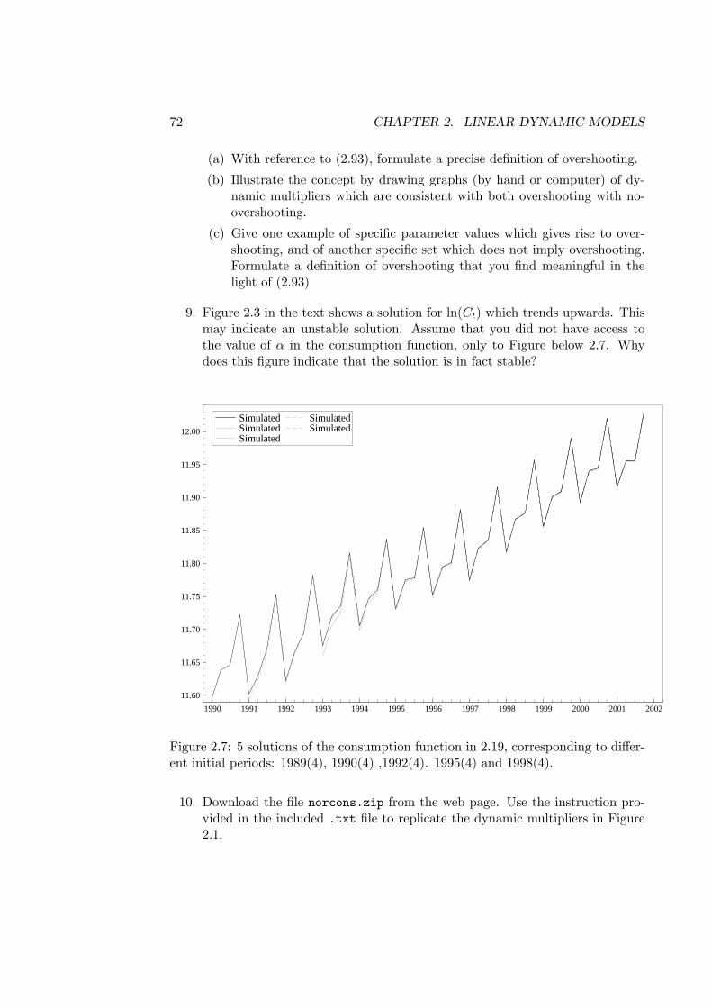
72 CHAPTER 2. LINEAR DYNAMIC MODELS
(a) With reference to (2.93), formulate a precise definition of overshooting.
(b) Illustrate the concept by drawing graphs (by hand or computer) of dy-namic multipliers which are consistent with both overshooting with no-overshooting.
(c) Give one example of specific parameter values which gives rise to over-shooting, and of another specific set which does not imply overshooting.Formulate a definition of overshooting that you find meaningful in thelight of (2.93)
9. Figure 2.3 in the text shows a solution for ln(Ct) which trends upwards. Thismay indicate an unstable solution. Assume that you did not have access tothe value of α in the consumption function, only to Figure below 2.7. Whydoes this figure indicate that the solution is in fact stable?
1990 1991 1992 1993 1994 1995 1996 1997 1998 1999 2000 2001 200211.60
11.65
11.70
11.75
11.80
11.85
11.90
11.95
12.00Simulated Simulated Simulated
Simulated Simulated
Figure 2.7: 5 solutions of the consumption function in 2.19, corresponding to differ-ent initial periods: 1989(4), 1990(4) ,1992(4). 1995(4) and 1998(4).
10. Download the file norcons.zip from the web page. Use the instruction pro-vided in the included .txt file to replicate the dynamic multipliers in Figure2.1.
Chapter 3
Wage-price dynamics
Theories of wage formation and of price setting are important inmacroeconomics since they represent the supply-side of macroeconomicmodels. In this chapter we discuss three alternative models of the supplyside: The wage bargain model, the Phillips curve and the New KeynesianPhillips curve. We note that the two first models are consistent withperception that firms and their (organized or unorganized) workers areengaged in a partly cooperative and partly conflictual sharing of the rentsgenerated by the operation of the firm. Despite this common ground,the models have notably different dynamic properties, and have differentpolicy implications. In the standard New Keynesian Phillips curve modelthere is no role for trade unions. That theory instead places singularemphasis on firms’ forward-looking behaviour.
3.1 Introduction
In economics the term ‘inflation’ generally describes the prevailing rate at which theprices of goods and services are increasing. It is commonplace that all prices tendto rise at broadly the same rate, because, when prices of domestic goods are rising,this will generally be true also of wages, and of the price of imported goods. This isbecause inflation in one sector of the economy permeates rapidly into other sectors.The phrase, a ‘high rate of inflation’ therefore usually describes a situation in whichthe money values of all goods in an economy are rising at a fast rate.
History shows many examples of countries which have been hit by extremelyhigh rates of inflation, so called hyperinflation. Any such episode is a result of crisisand disorganization in the economic and political system of a country, and of abreakdown in the public trust in the country’s monetary system. The typical caseis however that inflation can be moderately high for long periods of time withoutdoing serious damage to the stability of monetary institutions.
Nevertheless, even if we set aside the phenomenon of hyperinflation, it is generallyagreed that a high and volatile inflation rate is a cause of concern, and towards the
73
74 CHAPTER 3. WAGE-PRICE DYNAMICS
end of last century, the governments of the “Western world” invested heavily incurbing inflation. Institutional changes took place (crushing of labour unions inthe UK, revitalization of incomes policies in Norway, a new orientation of monetarypolicy, the European Union’s stability pact, etc.), and governments also allowedunemployment to rise to level not seen since the 2WW.
Was all this necessary, or were there other ways to curb inflation that wouldhave meant a lower toll in terms of unemployment? Finally, given that inflation hasnow become a prime target of economic policy, what is the inflation outlook andhow can inflation be controlled using the policy instruments that are recognized aslegitimate in liberalized economies? Answers to any of these important issues arenecessarily model dependent. By model dependency we mean that, before the answeris given, a view has been formulated, either explicitly or implicitly, about the majordeterminants of inflation and about which instruments are available for controllinginflation, and so forth. In this chapter we therefore discuss inflation models.
It is a well known fact that prices influence each other: wages follow the costof living index, which is based on prices on tradable and non-tradable goods, whichin their turn (and to varying extent) reflect labour costs that are determined bywage settlements of the past. Hence the ‘inflation spiral’ has a dynamic structurethat results from the interaction of several markets, where the markets for labourand goods are perhaps the two most important. Models of the dynamic structure ofwage and price setting are therefore of greatest importance, and they represent anarea where the modelling concepts of chapter 2 are indispensable.
In this chapter, we present two important models of wage and price settingbehaviour that are relevant to the inflation process of small open economies: thebargaining model, section 3.2.4, and the Phillips curve model, section 3.3. The mainpremise of the bargaining model is that firms and their (organized or unorganized)workers are engaged in a partly cooperative and partly conflictual sharing of therents generated by the operation of the firm. In Norway, a system of bargainingbased wage setting has been the framework both for analysis and policy decisionsfor decades.
The Phillips curve is covered by every textbook in macroeconomics, and in sec-tion 2.4.2 above we have already introduced a Phillips curve relationship, as anexample of how ADL models are applied in macroeconomics. In this chapter, wegive a fresh lick to the Phillips curve by comparing it with the bargaining modelof inflation. We show that the Phillips curve can be seen as a special case of thericher dynamics of the bargaining model, see section 3.4. The chapter also presentsome empirical evidence from the Norwegian economy, see section 3.5. Which modelreceives most support from the data? The Phillips curve or the bargaining model?
In the final section of the chapter we give an appraisal of the new KeynesianPhillips curve, which in a short period of time has become an important modelof the supply side in the models used to guide monetary policy, and which also isintegrated in the dynamic stochastic general equilibrium models, DSGEs.
3.2. WAGE BARGAINING AND INCOMPLETE COMPETITION. 75
3.2 Wage bargaining and incomplete competition.
In the course of the 1980s interesting developments took place in macroeconomics.First, the macroeconomic implications of imperfect competition with price-settingfirms were developed in several papers and books.1 Second, the economic theoryof labour unions, pioneered by Dunlop (1944), was extended and formalized in agame theoretic framework, see e.g., Nickell and Andrews (1983), Hoel and Nymoen(1988). Models of European unemployment, that incorporated elements from boththese developments, appeared in Layard and Nickell (1986), Layard et al. (1991),and Lindbeck (1993).
We refer to the overall framework as the Incomplete Competition Model (ICM)as in Bårdsen and Nymoen (2003) or, interchangeably, as the wage curve framework(as opposed to for example the Phillips curve model). Incomplete competition, isparticularly apt since the model’s defining characteristic is the explicit assumption ofimperfect competition in both product and labour markets.2 The ICM was quicklyincorporated into the supply side of macroconometric models, see Wallis (1993,1995), and purged European econometric models of the Phillips curve, at least untilthe arrival of the New Keynesian Phillips curve late in the 1990s (see below).
Time does not play an essential role in the standard bargaining models. Althoughthe theory is sometimes presented with reference to bargaining stages, real calendartime is not an explicit variable in the model. Hence, the interpretation of the wageequations rationalized by these theories is that they represent hypotheses aboutthe steady state. In line with this interpretation, and following the approach todynamics presented in the first two chapters, we first present the bargaining modelof wage setting as a theory of the steady state in section 3.2.1, and then present thefull equilibrium correction model in section 3.2.2.
3.2.1 A bargaining theory of the steady state wage
Since the focus of the book is the small open economy, we first establish the con-ceptual distinction between a tradables sector where firms act as price takers, ei-ther because they sell most of their produce on the world market, or because theyencounter strong foreign competition on their domestic sales markets, and a non-tradables sector where firms set prices as mark-ups on wage costs. There is mo-nopolistic competition among firms in this sector. The two sectors are dubbed theexposed (e) and sheltered (s) sectors of the economy.
We first need to establish some notation: Let Qe and Qs denote the producerprices in the two sectors. We assume that the consumer price index P is a weightedaverage of the two prices:
P = QφsQ
(1−φ)e 0 < φ < 1 (3.1)
1For example., Bruno (1979), and Blanchard and Kiyotaki (1987), Bruno and Sachs (1984) andBlanchard and Fisher (1989, Chapter 8)
2The ICM acrynom should not be taken to imply that the Phillips curve contain perfect com-petition, though.
76 CHAPTER 3. WAGE-PRICE DYNAMICS
where φ is a coefficient that reflects the weight of non-traded goods in private con-sumption,3. More realistically, we could add a third consumption good which is notproduced domestically, but with the cost of a more complicated notation.
Due to monopolistic competition, the steady state price in the sheltered sectoris proportional to the wage level Ws in that sector:
Qs =Ws
As. (3.2)
As is the average labour productivity. It is defined as As = Ys/Ls where Ys denotesoutput (measured as value added) in the non-tradable or sheltered sector, and Ls
denotes labour input (total number of hours worked). The parameter is determinedby the elasticity of demand facing each firm i with respect to the firm’s own price.It is a common to assume that the elasticity is independent of other firms prices,and that it is identical for all firms. It can be shown that if it is assume that theabsolute value of the elasticity of demand is larger than unity, then > 1 as well,and for that reason, is can be referred to as the price mark-up coefficient on wages.
In the two equations (3.1) and (3.2), Qe is by assumption exogenous (e-sectorfirms are price takers), and As is also exogenous and represents a technological trend.The wage level in the sheltered sector is determined by the following equation:
Ws =We (3.3)
saying that the sheltered sector wage is proportional to the wage in the exposedsector of the economy. To save notation, the proportionally factor has been setequal to unity.
The hourly wage level We is determined by bargaining between labour unionsand organizations representing firms. We define real profits, , asY
= Ye −We
QeLe = (1−
We
Qe
1
Ae)Ye.
Over the wage bargaining time horizon we assume, for simplicity that output Ye isequal to the capacity level. In this perspective, is possible that varying profitabilityresults in lower or increased capacity, hence we assume that Ye is a non-increasingfunction of real unit labour costs:
Ye = Ye(We/Qe
Ae), Y 0e ≤ 0. (3.4)
We assume that the wage We is settled in accordance with the principle of maxi-mizing the Nash-product:
(ν − ν0)fΠ1−f (3.5)
3For reference, due to the log-form, φ = xs/(1− xs) where xs is the share of non-traded goodsin consumption.
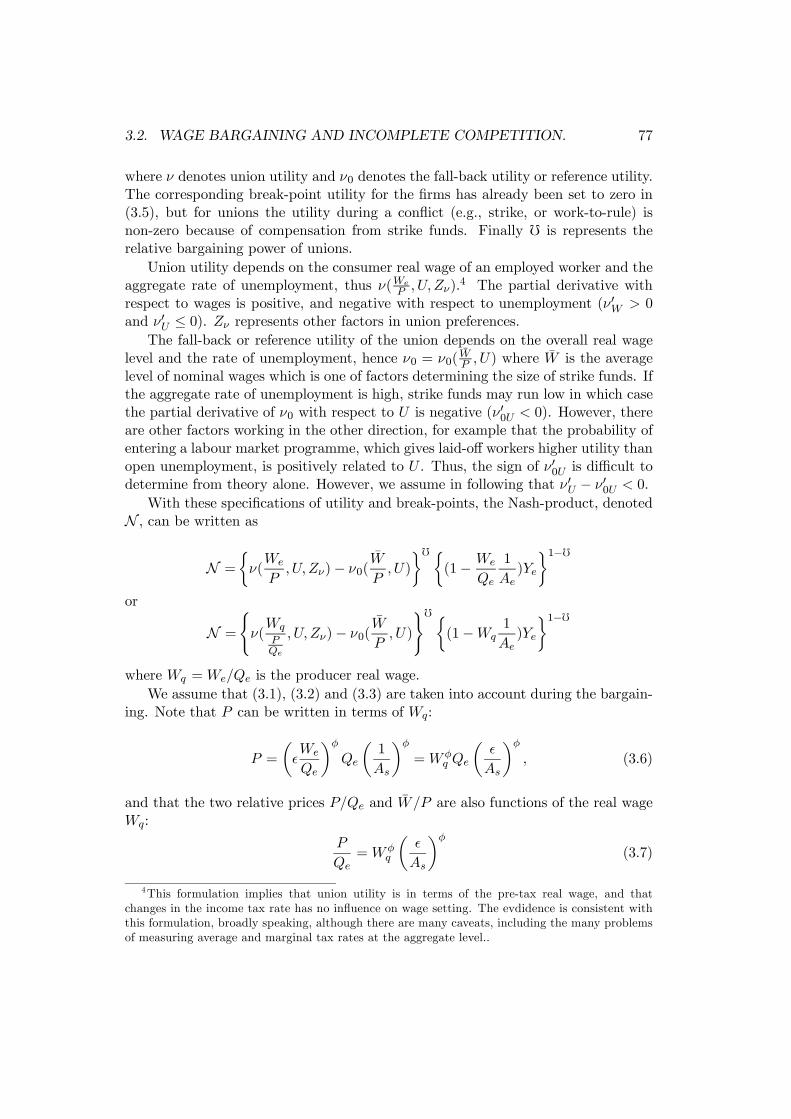
3.2. WAGE BARGAINING AND INCOMPLETE COMPETITION. 77
where ν denotes union utility and ν0 denotes the fall-back utility or reference utility.The corresponding break-point utility for the firms has already been set to zero in(3.5), but for unions the utility during a conflict (e.g., strike, or work-to-rule) isnon-zero because of compensation from strike funds. Finally f is represents therelative bargaining power of unions.
Union utility depends on the consumer real wage of an employed worker and theaggregate rate of unemployment, thus ν(We
P , U, Zν).4 The partial derivative withrespect to wages is positive, and negative with respect to unemployment (ν 0W > 0and ν0U ≤ 0). Zν represents other factors in union preferences.
The fall-back or reference utility of the union depends on the overall real wagelevel and the rate of unemployment, hence ν0 = ν0(
WP , U) where W is the average
level of nominal wages which is one of factors determining the size of strike funds. Ifthe aggregate rate of unemployment is high, strike funds may run low in which casethe partial derivative of ν0 with respect to U is negative (ν00U < 0). However, thereare other factors working in the other direction, for example that the probability ofentering a labour market programme, which gives laid-off workers higher utility thanopen unemployment, is positively related to U . Thus, the sign of ν00U is difficult todetermine from theory alone. However, we assume in following that ν 0U − ν00U < 0.
With these specifications of utility and break-points, the Nash-product, denotedN , can be written as
N =
½ν(We
P,U,Zν)− ν0(
W
P,U)
¾f ½(1− We
Qe
1
Ae)Ye
¾1−for
N =
(ν(WqPQe
, U, Zν)− ν0(W
P,U)
)f ½(1−Wq
1
Ae)Ye
¾1−fwhere Wq =We/Qe is the producer real wage.
We assume that (3.1), (3.2) and (3.3) are taken into account during the bargain-ing. Note that P can be written in terms of Wq:
P =
µWe
Qe
¶φ
Qe
µ1
As
¶φ
=Wφq Qe
µAs
¶φ
, (3.6)
and that the two relative prices P/Qe and W/P are also functions of the real wageWq:
P
Qe=Wφ
q
µAs
¶φ
(3.7)
4This formulation implies that union utility is in terms of the pre-tax real wage, and thatchanges in the income tax rate has no influence on wage setting. The evdidence is consistent withthis formulation, broadly speaking, although there are many caveats, including the many problemsof measuring average and marginal tax rates at the aggregate level..
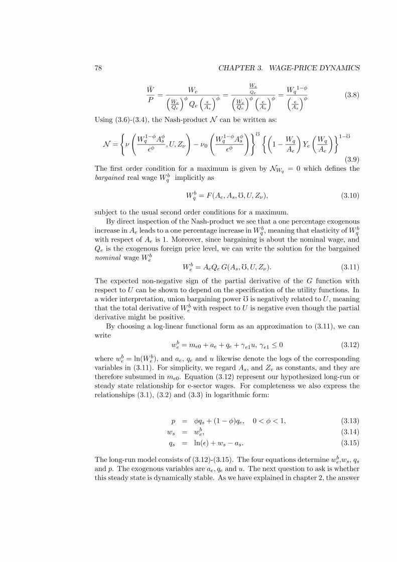
78 CHAPTER 3. WAGE-PRICE DYNAMICS
W
P=
We³WeQe
´φQe
³As
´φ = We
Qe³WeQe
´φ ³As
´φ = Wq1−φ³
As
´φ (3.8)
Using (3.6)-(3.4), the Nash-product N can be written as:
N =
(ν
ÃW 1−φ
q Aφs
φ, U, Zν
!− ν0
ÃW 1−φ
q Aφs
φ
!)f ½µ1− Wq
Ae
¶Ye
µWq
Ae
¶¾1−f(3.9)
The first order condition for a maximum is given by NWq = 0 which defines thebargained real wage W b
q implicitly as
W bq = F (Ae, As,f, U, Zν), (3.10)
subject to the usual second order conditions for a maximum.By direct inspection of the Nash-product we see that a one percentage exogenous
increase inAe leads to a one percentage increase inW bq , meaning that elasticity ofW
bq
with respect of Ae is 1. Moreover, since bargaining is about the nominal wage, andQe is the exogenous foreign price level, we can write the solution for the bargainednominal wage W b
e
W be = AeQeG(As,f, U, Zν). (3.11)
The expected non-negative sign of the partial derivative of the G function withrespect to U can be shown to depend on the specification of the utility functions. Ina wider interpretation, union bargaining power f is negatively related to U , meaningthat the total derivative of W b
e with respect to U is negative even though the partialderivative might be positive.
By choosing a log-linear functional form as an approximation to (3.11), we canwrite
wbe = me0 + ae + qe + γe1u, γe1 ≤ 0 (3.12)
where wbe = ln(W
be ), and ae, qe and u likewise denote the logs of the corresponding
variables in (3.11). For simplicity, we regard As, and Zv as constants, and they aretherefore subsumed in me0. Equation (3.12) represent our hypothesized long-run orsteady state relationship for e-sector wages. For completeness we also express therelationships (3.1), (3.2) and (3.3) in logarithmic form:
p = φqs + (1− φ)qe, 0 < φ < 1, (3.13)
ws = wbe, (3.14)
qs = ln( ) + ws − as. (3.15)
The long-run model consists of (3.12)-(3.15). The four equations determine wbe,ws, qs
and p. The exogenous variables are ae, qe and u. The next question to ask is whetherthis steady state is dynamically stable. As we have explained in chapter 2, the answer
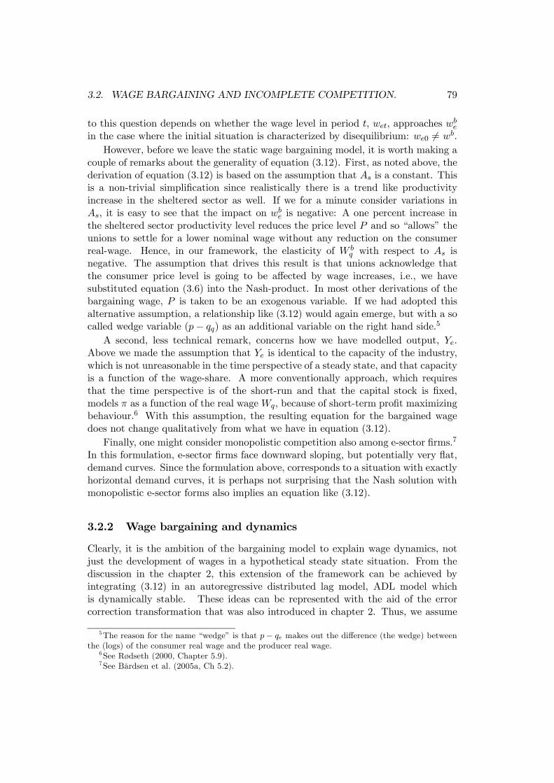
3.2. WAGE BARGAINING AND INCOMPLETE COMPETITION. 79
to this question depends on whether the wage level in period t, wet, approaches wbe
in the case where the initial situation is characterized by disequilibrium: we0 6= wb.However, before we leave the static wage bargaining model, it is worth making a
couple of remarks about the generality of equation (3.12). First, as noted above, thederivation of equation (3.12) is based on the assumption that As is a constant. Thisis a non-trivial simplification since realistically there is a trend like productivityincrease in the sheltered sector as well. If we for a minute consider variations inAs, it is easy to see that the impact on wb
e is negative: A one percent increase inthe sheltered sector productivity level reduces the price level P and so “allows” theunions to settle for a lower nominal wage without any reduction on the consumerreal-wage. Hence, in our framework, the elasticity of W b
q with respect to As isnegative. The assumption that drives this result is that unions acknowledge thatthe consumer price level is going to be affected by wage increases, i.e., we havesubstituted equation (3.6) into the Nash-product. In most other derivations of thebargaining wage, P is taken to be an exogenous variable. If we had adopted thisalternative assumption, a relationship like (3.12) would again emerge, but with a socalled wedge variable (p− qq) as an additional variable on the right hand side.5
A second, less technical remark, concerns how we have modelled output, Ye.Above we made the assumption that Ye is identical to the capacity of the industry,which is not unreasonable in the time perspective of a steady state, and that capacityis a function of the wage-share. A more conventionally approach, which requiresthat the time perspective is of the short-run and that the capital stock is fixed,models π as a function of the real wageWq, because of short-term profit maximizingbehaviour.6 With this assumption, the resulting equation for the bargained wagedoes not change qualitatively from what we have in equation (3.12).
Finally, one might consider monopolistic competition also among e-sector firms.7
In this formulation, e-sector firms face downward sloping, but potentially very flat,demand curves. Since the formulation above, corresponds to a situation with exactlyhorizontal demand curves, it is perhaps not surprising that the Nash solution withmonopolistic e-sector forms also implies an equation like (3.12).
3.2.2 Wage bargaining and dynamics
Clearly, it is the ambition of the bargaining model to explain wage dynamics, notjust the development of wages in a hypothetical steady state situation. From thediscussion in the chapter 2, this extension of the framework can be achieved byintegrating (3.12) in an autoregressive distributed lag model, ADL model whichis dynamically stable. These ideas can be represented with the aid of the errorcorrection transformation that was also introduced in chapter 2. Thus, we assume
5The reason for the name “wedge” is that p− qe makes out the difference (the wedge) betweenthe (logs) of the consumer real wage and the producer real wage.
6See Rødseth (2000, Chapter 5.9).7See Bårdsen et al. (2005a, Ch 5.2).
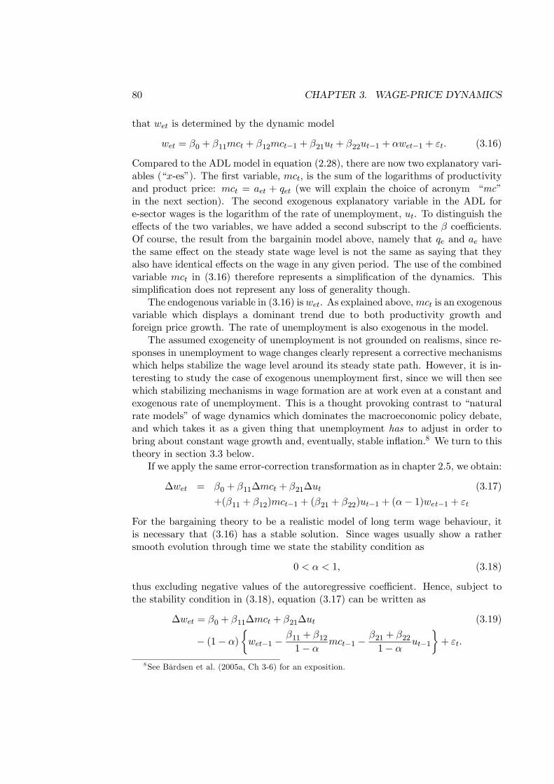
80 CHAPTER 3. WAGE-PRICE DYNAMICS
that wet is determined by the dynamic model
wet = β0 + β11mct + β12mct−1 + β21ut + β22ut−1 + αwet−1 + εt. (3.16)
Compared to the ADL model in equation (2.28), there are now two explanatory vari-ables (“x-es”). The first variable, mct, is the sum of the logarithms of productivityand product price: mct = aet + qet (we will explain the choice of acronym “mc”in the next section). The second exogenous explanatory variable in the ADL fore-sector wages is the logarithm of the rate of unemployment, ut. To distinguish theeffects of the two variables, we have added a second subscript to the β coefficients.Of course, the result from the bargainin model above, namely that qe and ae havethe same effect on the steady state wage level is not the same as saying that theyalso have identical effects on the wage in any given period. The use of the combinedvariable mct in (3.16) therefore represents a simplification of the dynamics. Thissimplification does not represent any loss of generality though.
The endogenous variable in (3.16) iswet. As explained above,mct is an exogenousvariable which displays a dominant trend due to both productivity growth andforeign price growth. The rate of unemployment is also exogenous in the model.
The assumed exogeneity of unemployment is not grounded on realisms, since re-sponses in unemployment to wage changes clearly represent a corrective mechanismswhich helps stabilize the wage level around its steady state path. However, it is in-teresting to study the case of exogenous unemployment first, since we will then seewhich stabilizing mechanisms in wage formation are at work even at a constant andexogenous rate of unemployment. This is a thought provoking contrast to “naturalrate models” of wage dynamics which dominates the macroeconomic policy debate,and which takes it as a given thing that unemployment has to adjust in order tobring about constant wage growth and, eventually, stable inflation.8 We turn to thistheory in section 3.3 below.
If we apply the same error-correction transformation as in chapter 2.5, we obtain:
∆wet = β0 + β11∆mct + β21∆ut (3.17)
+(β11 + β12)mct−1 + (β21 + β22)ut−1 + (α− 1)wet−1 + εt
For the bargaining theory to be a realistic model of long term wage behaviour, itis necessary that (3.16) has a stable solution. Since wages usually show a rathersmooth evolution through time we state the stability condition as
0 < α < 1, (3.18)
thus excluding negative values of the autoregressive coefficient. Hence, subject tothe stability condition in (3.18), equation (3.17) can be written as
∆wet = β0 + β11∆mct + β21∆ut (3.19)
− (1− α)
½wet−1 −
β11 + β121− α
mct−1 −β21 + β221− α
ut−1
¾+ εt.
8See Bårdsen et al. (2005a, Ch 3-6) for an exposition.
3.2. WAGE BARGAINING AND INCOMPLETE COMPETITION. 81
To reconcile this with the steady state relationship (3.12), we define
γe,1 =β21 + β221− α
,
saying that the elasticity of wb with respect to the rate of unemployment is identicalto the long—run multiplier of the actual wage wet with respect to ut, and then imposethe following restriction on the coefficient of mct−1:
β11 + β12 = (1− α) (3.20)
since (3.12) implies that the long-run multiplier with respect to mc is unity. Then(3.19) becomes
∆wet = β0 + β11∆mct + β21∆ut (3.21)
−(1− α) {wet−1 −mct−1 − γe1ut−1}+ εt
which is an example of the homogenous ECM of section 2.3. The short-run multiplierwith respect to mct is of course β11, which can be considerably smaller than unitywithout violating the long-run relationship (3.12).
The formulation in (3.21) is an equilibrium correction model, ECM exactly be-cause the term in brackets captures that wage growth in period t partly corrects lastperiod’s deviation from the long-run equilibrium wage level. We can write it as
∆wet = β00 + β11∆mct + β21∆ut (3.22)
−(1− α)nwe − wb
e
ot−1
+ εt
where wbe is given in (3.12) and β
00 is given as β
00 = β0 − (1− α)me0.
You should check that the derivations above parallel those given in chapter 2,equation (2.31)-(2.34) in particular. Hence the following equation is equivalent to(3.21) and (3.22)
∆wet = β00 + β11∆mct + β21∆ut (3.23)
−(1− α) {we −mct−1 − γe1ut−1 −me0}+ εt,
we only need to keep in mind that β00 = β0 − (1− α)me0 as explained.Subject to the condition 0 < α < 1 stated above, wage growth is seen to bring
the wage level in the direction of the bargained wage wbe. For example, assume that
the sum of price and productivity growth is constant so that ∆mct = gmc, that therate of unemployment is constant, ∆ut = 0, and that there is no new shockt, εt = 0.If there is disequilibrium in period t−1, for example
©we − wb
e
ªt−1 > 0, wage growth
from t− 1 to t will be reduced, and this leads to©we − wb
e
ªt<©we − wb
e
ªt−1 in the
next period.
82 CHAPTER 3. WAGE-PRICE DYNAMICS
Finally in the steady state equilibrium, with a prevailing constant rate of un-employment, and no random shocks, then wt−1 = wb
et−1 as well as wt = wbt , and
steady state wage growth is therefore ∆wet = ∆wbet = gmc. At this point teh reader
may have noted an apparent inconsistency, since, given these assumptions, the ECM(3.23) gives:
∆wet = β00 + β11gmc,
and not ∆wet = gmc as implied by the steady-state path for the wage level. However,this paradox is resolved by noting that the original constant term β0 in the ADLcan be defined to be
β0 = (1− α)me0 − (β11 − 1)gmc. (3.24)
If we invoke this definition of β0, the dynamic equation (3.23) is seen to give ∆wet =(1 − α)me0 − (β11 − 1)gmc − (1 − α)me0 + β11gmc = gmc, which is consistent with∆wet = ∆w
bet = gmc in the steady state. At first it may seem a to be a suspect
trick to define the constant term of the ECM in the way we do in equation (3.24).Without going into details this is however not the case, and the definition in (3.24)is innocuous. One way to think about this is that if β0 measured something differentthan (3.24) our theory would not account for the systematic part of wage growth,and in that case, a different ECM should have been formulated from the outset. Forthose with a background in econometrics, (3.24) is seen to correspond to formulatinga regression equation by subtracting the means of the variables on both sides of theequation, an operation which does not affect the equation or the estimation resultsobtained.
3.2.3 Wage bargaining and inflation
So far, we have looked at only e-sector wage formation, and not inflation as such.To sketch the theory’s implication for inflation, we need to reconsider the threeequations (3.13)-(3.15). Equation (3.13) is a definition equation that holds not onlyin the long run, but also in each time period. Hence, we have
pt = φqst + (1− φ)qet
or in terms of growth rates:
∆pt = φ∆qst + (1− φ)∆qet. (3.25)
The two equations (3.14), for the s-sector wage, and (3.15), for the s-sector pricelevel, have a different interpretation. They are hypotheses about the steady state,and as we learned already in the opening chapter of the book, adding time subscriptsto these equations entail that we assume that s-sector price and wage formation arecharacterized by instantaneous adjustment (infinite speed of adjustment). This isclearly unrealistic, since there is no reason why adjustment lags and friction shouldnot be important for wage and price adjustments in the sheltered sector. Hence, it is
3.2. WAGE BARGAINING AND INCOMPLETE COMPETITION. 83
only in order to simplify the model as much as possible that we write the equationsfor ∆wst and ∆qst as
∆wst = ∆wet, and (3.26)
∆qst = ∆wet −∆aet. (3.27)
Equation (3.23) for e-sector wage growth and (3.25)-(3.27) are 4 equations whichdetermine the endogenous variables wet, wst, qst and pt as functions of initial con-ditions and given values for exogenous variables mct, ut and εt. The exogenous andpre-determined variables are wet−1, mct−1 and ut−1. The model is a recursive sys-tem of equations: The wage growth rate in the exposed sector is determined first,from (3.23) and then the other growth rates follow recursively
Specifically, the reduced form equation for the rate of inflation, ∆pt, is found tobe:
∆pt = φβ00 (3.28)
+(φβ11 + (1− φ))∆qe,t + φβ21∆ut
+φβ11∆aet − φ∆ast
−φ(1− α) {wet−1 −mct−1 − γe1ut−1 −me0}+φεt
showing that the bargaining model implies the following explanation of inflation ina small-open economy:
1. Autonomous inflation: φβ00,
2. “Imported inflation”: (φβ11 + (1− φ))∆qet
3. Shock to unemployment: φβ21∆ut
4. Productivity growth: φβ11∆aet − φ∆ast,
5. e-sector equilibrium correction: −φ(1− α) {we.t−1 −mct−1 − γe1ut−1 −me0}
6. random shocks: φεt
In order to get some idea about the size of these factors, we may set the share ofnon-traded goods in consumption to 0.4. Then φ = 0.67, and setting β11 = 0.5 givesa coefficient of ∆qet of 0.66. Foreign inflation in the range of 1%− 5% is of coursenot uncommon, and our model implies that a 3% inflation abroad implies about2% “imported inflation”. The coefficient of ∆aet is 0.33, and for ∆ast we obtain−0.67. The net-effect of productivity growth rates at around 2% may therefore berather small. Note the implication that increased productivity in the exposed sectorof the economy increases inflation. It occurs because e-sector productivity growthincreases the bargained wage in that sector, which inflicts price increases in thesheltered sector via the assumption of relative wage stabilization.
84 CHAPTER 3. WAGE-PRICE DYNAMICS
Equilibrium correction in the exposed sector represents a numerically significantfactor in this model. With the chosen parameter values, and setting α = 0.7 inthe wage equation, the coefficient of {we.t−1 −mct−1 − γe1ut−1 −me0} in equation(3.28) becomes 0.2. The interpretation is that a 1 percentage point deviation fromthe the steady state wage in period t−1 leads to a reduction of the period t inflationrate of 0.2 percentage points, ceteris paribus.
As noted, our derivation of the bargaining model inflation equation is very styl-ized. Practical use of the framework needs to represent ∆wst and ∆qst by separateequilibrium correction equations, and not impose instantaneous adjustment as wehave done in order to simplify. However, also in derivations which include more real-istic models of sheltered sector wage and price adjustment, many of the properties of(3.28) will continue to hold true. For example the strong role of imported inflation,the sign reversal of the two productivity terms, and the role of equilibrium-correctionin exposed sector wage setting.
Above, we have repeatedly noted that the inflation model is recursive. In actualwage setting, compensation for cost-of-living increases is always one of the issues.Hence, to increase the degree of realism of the model one would, in most cases,want to include ∆pt in the dynamic equation of exposed sector wages setting, witha positive coefficient (less than one, though). Clearly, with this generalization of themodel, the inflation model is no longer a recursive system, since instead of (3.23),we have:
∆wet = β00 + β11∆mct + β21∆ut + β31∆pt (3.29)
−(1− α) {wet−1 −mct−1 − γe1ut−1 −me0}+ εt.
However, since inflation can be expresses as:
∆pt = φ∆wet − φ∆ast + (1− φ)∆qet
we can derive the following semi-reduced form for ∆wet:
∆wet = β00 + β11∆mct + β21∆ut + β41∆ast + β51∆qet (3.30)
−^(1− α) {wet−1 −mct−1 − γe1ut−1 −me0}+ εt.
where the coefficient with aneare the original coefficients of (3.29) divided by (1−β31φ), and β41 = −β31φ/(1− β31φ), β51 = β31(1− φ)/(1− β31φ). By using (3.30)instead of (3.29) in the system-of-equations, the recursive nature of the model is putback in place.
3.2.4 The Norwegian model of inflation
The Norwegian model of inflation was formulated in the 1960s, several decadesbefore the formal bargaining approach was applied to wage setting9. It soon became
9In fact there were two models, a short-term multisector model, and the long-term two sectormodel that we re-construct using modern terminology in this chapter. The models were formulated
3.2. WAGE BARGAINING AND INCOMPLETE COMPETITION. 85
the framework for both medium term forecasting and normative judgements about“sustainable” centrally negotiated wage growth in Norway.10 However, it is notthe historical importance of the Norwegian model which is our concern here, butinstead that the Norwegian model of inflation is consistent with the implications ofthe bargaining model. Moreover, while the interpretation of the modern bargainingmodel is often left hanging “in the air”, with some researchers even viewing it as amodel that is relevant in the short-run, the Norwegian model was originally explicitlyformulated as a long-run model. Consistent with this is the Norwegian model’scareful analysis of the potentially numerous equilibrating mechanisms, but also themultitude of disequilibrating shocks that realistically characterizes wage dynamicsin the short-run. From this point of view, the Norwegian model is a more generalmodel of bargaining dominated wage evolution.
Another name for the Norwegian model is the main-course model for wages,since a joint trend made up of productivity and foreign prices define the scope forwage growth, i.e., the main-course followed by the wage level through time. In thefollowing, we use the names main-course model and Norwegian model of inflationinterchangeably.
3.2.4.1 A direct motivation for long-run wage and price relationships
In the same way as above, a central distinction is drawn between a tradables sectorwhere firms act as price takers, and a non-tradables sector where firms set prices asmark-ups on wage costs. In the same manner as above, the two sectors are dubbedthe exposed (e) and sheltered (s) sectors of the economy.
The model’s main propositions are, first, that exposed sector wage growth willfollow a long-run tendency defined by the exogenous price and productivity trendswhich characterize that sector. The joint productivity and price trend is called themain-course of e-sector wage development. The relationship corresponds to equation(3.12), for the bargained wage. Second, it is assumed that the relative wage betweenthe two sectors are constant in the long-run, as already introduced in equation (3.3).Third, the development of the price level in the s-sector is a mark-up on the unit-labour costs in that sector, as captured by (3.2). In this section we concentrate onhow the first proposition is rationalized in the seminal contribution by Odd Aukrust,from 1977.11
in 1966 in two reports by a group of economists who were called upon by the Norwegian governmentto provide background material for that year’s round of negotiations on wages and agriculturalprices. The group (Aukrust, Holte and Stolzt) produced two reports. The second (dated October20 1966, see Aukrust (1977)) contained the long-term model that we refer to as the main-coursemodel. Later, there was similar development in e.g., Sweden, see Edgren et al. (1969) and theNetherlands, see Driehuis and de Wolf (1976).In later usage the distinction between the short and long-term models seems to have become
blurred, in what is often referred to as the Scandinavian model of inflation. We acknowledgeAukrust’s clear exposition and distinction in his 1977 paper, and use the terminology Norwegianmain-course model for the long-term version of his theoretical framework.10On the role of the main-course model in Norwegian economic planning, see Bjerkholt (1998).11Aukrust (1977).
86 CHAPTER 3. WAGE-PRICE DYNAMICS
Recall that the wage share of value added output in the e-sector is
WeLe
QeYe=
We
QeAe, where average labour productivity is given as Ae =
YeLe.
Correspondingly, the rate of profit is
QeYe −WeLe
QeYe= 1− We
QeAe.
It is reasonable to assume that in order to attract the investments needed to maintaincompetitiveness and employment in the e-sector, a certain normal rate of profit hasto be met, at least in the long term. Since there is a one-to-one link between theprofit rate and the wage share, there is also a certain maintainable level of wageshare. Denote this long-run wage shareMe, and assume that both the product priceand productivity are exogenous variables. We can now formulate what we mightcall the main-course proposition:
W ∗e =MeQeAe, (3.31)
where W ∗e denotes the long-run equilibrium wage level consistent with the two as-
sumptions of exogenous price and productivity, and the existence of a normal wageshare. It is practical to take logs,
H1mc: w∗e = qe + ae +me, (3.32)
and use the marker H1mc to indicates that this is the first hypothesis of the theory.As ususal we identify the long-run equilibrium wage level, W ∗
e or (in log) w∗e , withthe steady state wage level. Equation (3.32) therefore captures that the long-runelasticities of the wage level with respect to productivity and price are both unity.
Equation (3.32) has a very important implication for actual data of wages, pricesand productivity in the e−sector: Since data for qe and ae show trend-like growthover time, actual time series data for the nominal wage, wet, should also show adominant positive growth around a trend defined by price and productivity. Ifthis is not the case, then w∗e , cannot be the equilibrium to which the actual wageconverges in a steady state.
The joint trend made up of productivity and foreign prices, traces out a cen-tral tendency for wage growth, it represents a long-run sustainable scope for wagegrowth. Aukrust (1977) aptly refers to this joint trend as the main-course for wagedetermination in the exposed industries.12 For reference we therefore define themain-course variable (in logs) as
mc = ae + qe. (3.33)
It is instructive to see, by way of citation, that Aukrust meant exactly what we haveasserted, namely that equation (3.32) is a long-run relationship corresponding to asteady state situation. Consider for example the following quotation:12The essence of the statistical interpretation of the theory is captured by the hypothesis of so
called cointegration between we and mc see Nymoen (1989) and Rødseth and Holden (1990)).
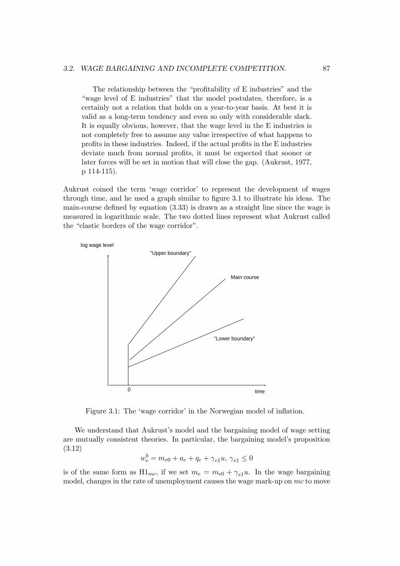
3.2. WAGE BARGAINING AND INCOMPLETE COMPETITION. 87
The relationship between the “profitability of E industries” and the“wage level of E industries” that the model postulates, therefore, is acertainly not a relation that holds on a year-to-year basis. At best it isvalid as a long-term tendency and even so only with considerable slack.It is equally obvious, however, that the wage level in the E industries isnot completely free to assume any value irrespective of what happens toprofits in these industries. Indeed, if the actual profits in the E industriesdeviate much from normal profits, it must be expected that sooner orlater forces will be set in motion that will close the gap. (Aukrust, 1977,p 114-115).
Aukrust coined the term ‘wage corridor’ to represent the development of wagesthrough time, and he used a graph similar to figure 3.1 to illustrate his ideas. Themain-course defined by equation (3.33) is drawn as a straight line since the wage ismeasured in logarithmic scale. The two dotted lines represent what Aukrust calledthe “elastic borders of the wage corridor”.
log wage level
time
Main course
"Upper boundary"
"Lower boundary"
0
Figure 3.1: The ‘wage corridor’ in the Norwegian model of inflation.
We understand that Aukrust’s model and the bargaining model of wage settingare mutually consistent theories. In particular, the bargaining model’s proposition(3.12)
wbe = me0 + ae + qe + γe1u, γe1 ≤ 0
is of the same form as H1mc, if we set me = me0 + γe1u. In the wage bargainingmodel, changes in the rate of unemployment causes the wage mark-up onmc to move

88 CHAPTER 3. WAGE-PRICE DYNAMICS
up or down. In a similar way, the normal rate of profit in the main-course modelis conditioned by economic, social and institutional factors. A long term change inthe rate of unemployment is one of the factors that can shift the sustainable profitrate.13 Therefore, it is fully consistent with the gist of Aukrust’s model that wereplace H1mc by the more general hypothesis:
H1gmc w∗e = me0 +mc+ γe1u.
As mentioned above, there are two other long-run propositions which are part ofAukrust’s theory. The first is an assumption about a constant relative wage betweenthe two sectors, and the second is a normal sustainable wage share also in thesheltered sector of the economy. We dub these two additional propositions H2mc
and H3mc respectively:
H2mc w∗s − w∗e = mse,H3mc w∗s − q∗s − as = ms,
mse is the log of the long-run ratio between e-sector and s-sector wages. as is theexogenous productivity trend in the sheltered sector, and ms is the (log) of theequilibrium wage rate in the sheltered sector. With reference to section 3.2.1, inthat model, mse = ln(1) and ms = − ln( ).
Note that, if the long-run wage in the exposed sector is determined by the exoge-nous main course, then H2mc determines the long-run wage in the sheltered sector,and H3mc in turn determines the long-run price level of the sheltered sector. Hence,re-arranging H3mc, gives
q∗s = w∗s − as −ms
which is similar to theories of so called normal cost pricing: the price is set as amark-up on average labour costs, in accordance with (3.15) above.
3.2.4.2 Dynamic adjustment in the Norwegian model
As we have seen, Aukrust was clear about two things. First, the main-course re-lationship for e-sector wages should be interpreted as a long-run tendency, not asa relationship that governs wage development on a year to year basis. Hence, thetheory makes us anticipate that actual observations of e-sector wages will fluctuatearound the theoretical main-course. Second, if e-sector wages deviate too much fromthe long-run tendency, we expect that forces will begin to act on wage setting so thatadjustments are made in the direction of the main-course. For example, profitabilitybelow the main-course level will tend to lower wage growth, either directly or aftera period of higher unemployment. In Aukrust’s words:
13No doubt, Aukrust’s formulation, without unemployment as an explicit variable, was condi-tioned by the realities of the Norwegian economy of the 1960s, where unemployment had beenconstant at a low level since the ende of WW2 in line with poltical priorites..
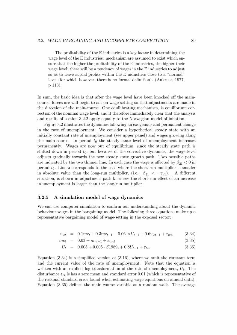
3.2. WAGE BARGAINING AND INCOMPLETE COMPETITION. 89
The profitability of the E industries is a key factor in determining thewage level of the E industries: mechanism are assumed to exist which en-sure that the higher the profitability of the E industries, the higher theirwage level; there will be a tendency of wages in the E industries to adjustso as to leave actual profits within the E industries close to a “normal”level (for which however, there is no formal definition). (Aukrust, 1977,p 113).
In sum, the basic idea is that after the wage level have been knocked off the main-course, forces are will begin to act on wage setting so that adjustments are made inthe direction of the main-course. One equilibrating mechanism, is equilibrium cor-rection of the nominal wage level, and it therefore immediately clear that the analysisand results of section 3.2.2 apply equally to the Norwegian model of inflation.
Figure 3.2 illustrates the dynamics following an exogenous and permanent changein the rate of unemployment: We consider a hypothetical steady state with aninitially constant rate of unemployment (see upper panel) and wages growing alongthe main-course. In period t0 the steady state level of unemployment increasespermanently. Wages are now out of equilibrium, since the steady state path isshifted down in period t0, but because of the corrective dynamics, the wage leveladjusts gradually towards the new steady state growth path. Two possible pathsare indicated by the two thinner line. In each case the wage is affected by β21 < 0 inperiod t0. Line a corresponds to the case where the short-run multiplier is smallerin absolute value than the long-run multiplier, (i.e.,−β21 < −γe1). A differentsituation, is shown in adjustment path b, where the short-run effect of an increasein unemployment is larger than the long-run multiplier.
3.2.5 A simulation model of wage dynamics
We can use computer simulation to confirm our understanding about the dynamicbehaviour wages in the bargaining model. The following three equations make up arepresentative bargaining model of wage-setting in the exposed sector:
wet = 0.1mct + 0.3mct−1 − 0.06 lnUt−1 + 0.6wet−1 + εwt, (3.34)
mct = 0.03 +mct−1 + εmct (3.35)
Ut = 0.005 + 0.005 · S1989t + 0.8Ut−1 + εUt (3.36)
Equation (3.34) is a simplified version of (3.16), where we omit the constant termand the current value of the rate of unemployment. Note that the equation iswritten with an explicit log transformation of the rate of unemployment, Ut. Thedisturbance εet is has a zero mean and standard error 0.01 (which is representative ofthe residual standard error found when estimating wage equations on annual data).Equation (3.35) defines the main-course variable as a random walk. The average
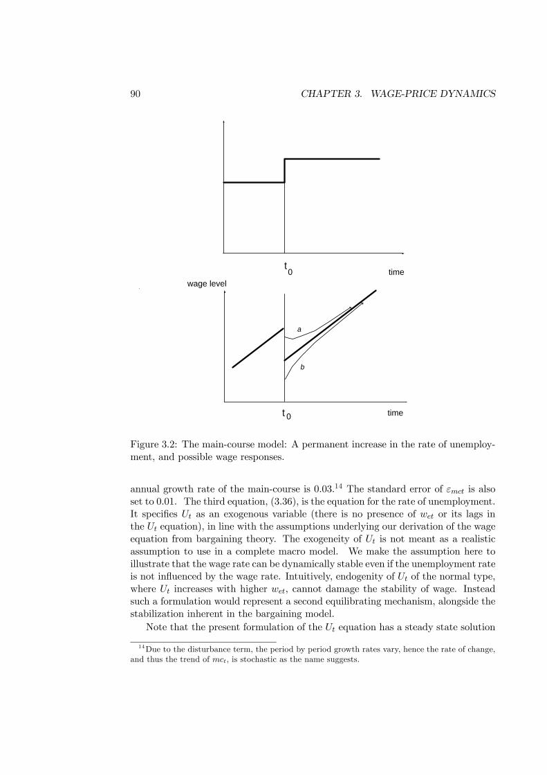
90 CHAPTER 3. WAGE-PRICE DYNAMICS
t0
t 0
timewage level
time
a
b
Figure 3.2: The main-course model: A permanent increase in the rate of unemploy-ment, and possible wage responses.
annual growth rate of the main-course is 0.03.14 The standard error of εmct is alsoset to 0.01. The third equation, (3.36), is the equation for the rate of unemployment.It specifies Ut as an exogenous variable (there is no presence of wet or its lags inthe Ut equation), in line with the assumptions underlying our derivation of the wageequation from bargaining theory. The exogeneity of Ut is not meant as a realisticassumption to use in a complete macro model. We make the assumption here toillustrate that the wage rate can be dynamically stable even if the unemployment rateis not influenced by the wage rate. Intuitively, endogenity of Ut of the normal type,where Ut increases with higher wet, cannot damage the stability of wage. Insteadsuch a formulation would represent a second equilibrating mechanism, alongside thestabilization inherent in the bargaining model.
Note that the present formulation of the Ut equation has a steady state solution
14Due to the disturbance term, the period by period growth rates vary, hence the rate of change,and thus the trend of mct, is stochastic as the name suggests.
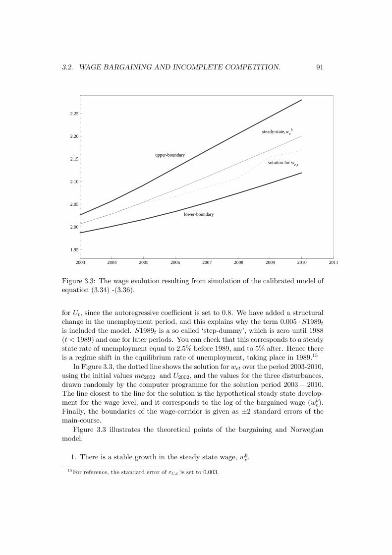
3.2. WAGE BARGAINING AND INCOMPLETE COMPETITION. 91
2003 2004 2005 2006 2007 2008 2009 2010 2011
1.95
2.00
2.05
2.10
2.15
2.20
2.25
upper-boundary
lower-boundary
steady-state, web
solution for we ,t
Figure 3.3: The wage evolution resulting from simulation of the calibrated model ofequation (3.34) -(3.36).
for Ut, since the autoregressive coefficient is set to 0.8. We have added a structuralchange in the unemployment period, and this explains why the term 0.005 · S1989tis included the model. S1989t is a so called ‘step-dummy’, which is zero until 1988(t < 1989) and one for later periods. You can check that this corresponds to a steadystate rate of unemployment equal to 2.5% before 1989, and to 5% after. Hence thereis a regime shift in the equilibrium rate of unemployment, taking place in 1989.15
In Figure 3.3, the dotted line shows the solution for wet over the period 2003-2010,using the initial values mc2002 and U2002, and the values for the three disturbances,drawn randomly by the computer programme for the solution period 2003 − 2010.The line closest to the line for the solution is the hypothetical steady state develop-ment for the wage level, and it corresponds to the log of the bargained wage (wb
e).Finally, the boundaries of the wage-corridor is given as ±2 standard errors of themain-course.
Figure 3.3 illustrates the theoretical points of the bargaining and Norwegianmodel.
1. There is a stable growth in the steady state wage, wbe.
15For reference, the standard error of εU,t is set to 0.003.
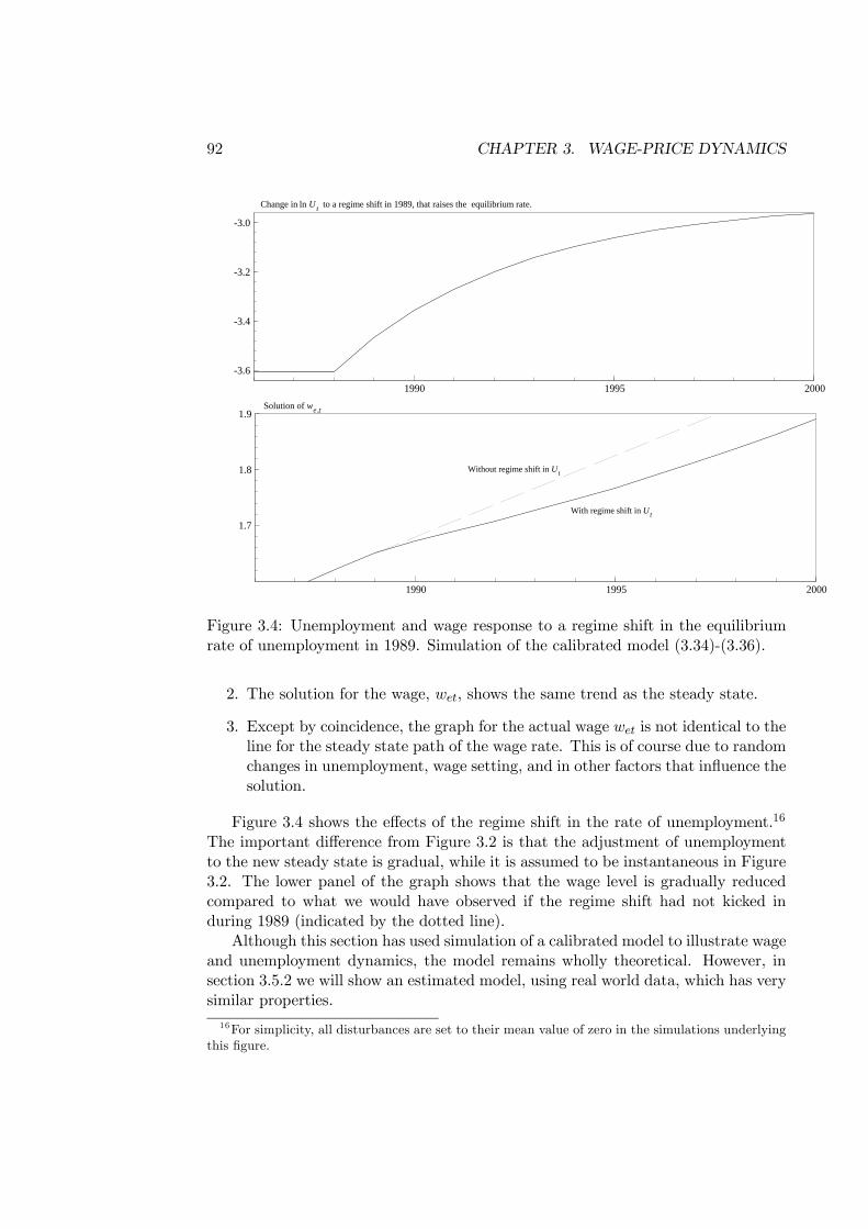
92 CHAPTER 3. WAGE-PRICE DYNAMICS
1990 1995 2000
1.7
1.8
1.9Solution of we ,t
With regime shift in Ut
Without regime shift in Ut
1990 1995 2000
-3.6
-3.4
-3.2
-3.0
Change in ln Ut to a regime shift in 1989, that raises the equilibrium rate.
Figure 3.4: Unemployment and wage response to a regime shift in the equilibriumrate of unemployment in 1989. Simulation of the calibrated model (3.34)-(3.36).
2. The solution for the wage, wet, shows the same trend as the steady state.
3. Except by coincidence, the graph for the actual wage wet is not identical to theline for the steady state path of the wage rate. This is of course due to randomchanges in unemployment, wage setting, and in other factors that influence thesolution.
Figure 3.4 shows the effects of the regime shift in the rate of unemployment.16
The important difference from Figure 3.2 is that the adjustment of unemploymentto the new steady state is gradual, while it is assumed to be instantaneous in Figure3.2. The lower panel of the graph shows that the wage level is gradually reducedcompared to what we would have observed if the regime shift had not kicked induring 1989 (indicated by the dotted line).
Although this section has used simulation of a calibrated model to illustrate wageand unemployment dynamics, the model remains wholly theoretical. However, insection 3.5.2 we will show an estimated model, using real world data, which has verysimilar properties.16For simplicity, all disturbances are set to their mean value of zero in the simulations underlying
this figure.
3.2. WAGE BARGAINING AND INCOMPLETE COMPETITION. 93
3.2.6 The main-course model and the Scandinavian model of infla-tion
So far in this chapter we have discussed two theoretical models of wage dynamics andinflation which, although they originated in different historical period, are mutuallyconsistent. Both models are genuine dynamic models since they are built on anexplicit distinction between the short-run and the long-run. The distinction betweenlong-term steady state propositions and dynamics has not always been made clear,though. This is true for the Scandinavian model, which the main-course model isoften confounded with.
The Scandinavian model, see Rødseth (2000, Ch 7.6), specifies the same threeunderlying assumptions as the main-course model: H1mc (we do not need the ex-tended version of the hypothesis for the point we wish to make here), H2mc andH3mc. But the distinction between long-run and dynamics is blurred in the Scandi-navian model. Hence, for example, the dynamic equation for e-sector wages in theScandinavian model is usually written as:
∆we,t = β0 +∆mct,
(without a disturbance term for simplicity) which is seen to place the rather unreal-istic restriction of α = 1 on e-sector wage dynamics. Hence, the Scandinavian modelspecification can only be expected to be reasonable if the time period subscript trefers to a span of several years, so that ∆we,t and ∆mct refer to for example 10years averages of the two growth rates.17
3.2.7 Wage-price curves and the NAIRU/natural rate of unemploy-ment
Most modern textbooks in macroeconomics contain models of trade unions and firmbehaviour. The gist of these models is that firms attempt to mark-up up their priceson unit labour costs, while workers and unions on their part strive to make their realwage reflect the profitability of the firms, thus their real wage claim is a mark-up onproductivity. Hence, there is an important and interesting conflict between workersand firms: Both parties are interested in the size of the real wage, but their goalsare usually different. Neither of the parties have perfect control over the real wage:Unions have only limited influence on the real wage since their channel of influenceis the bargaining process, which is about the size of nominal wage increases. Firmsalso influences the nominal wage as long as they are part of the bargaining, moreoverthey have a strong channel of influence on the real wage since they decide the size ofprice adjustment unilaterally through mark-up pricing. Nevertheless, the real wageis neither perfectly controlled nor perfectly foreseeable by the firms.
Although it might already be obvious to the reader, the bargaining model whichwe have set out above (and therefore also the main-course model) fits into this
17For an exposition and appraisal of the Scandinavian model, in terms of contemporary macro-economics, see Rødseth (2000, Chapter 7.6)
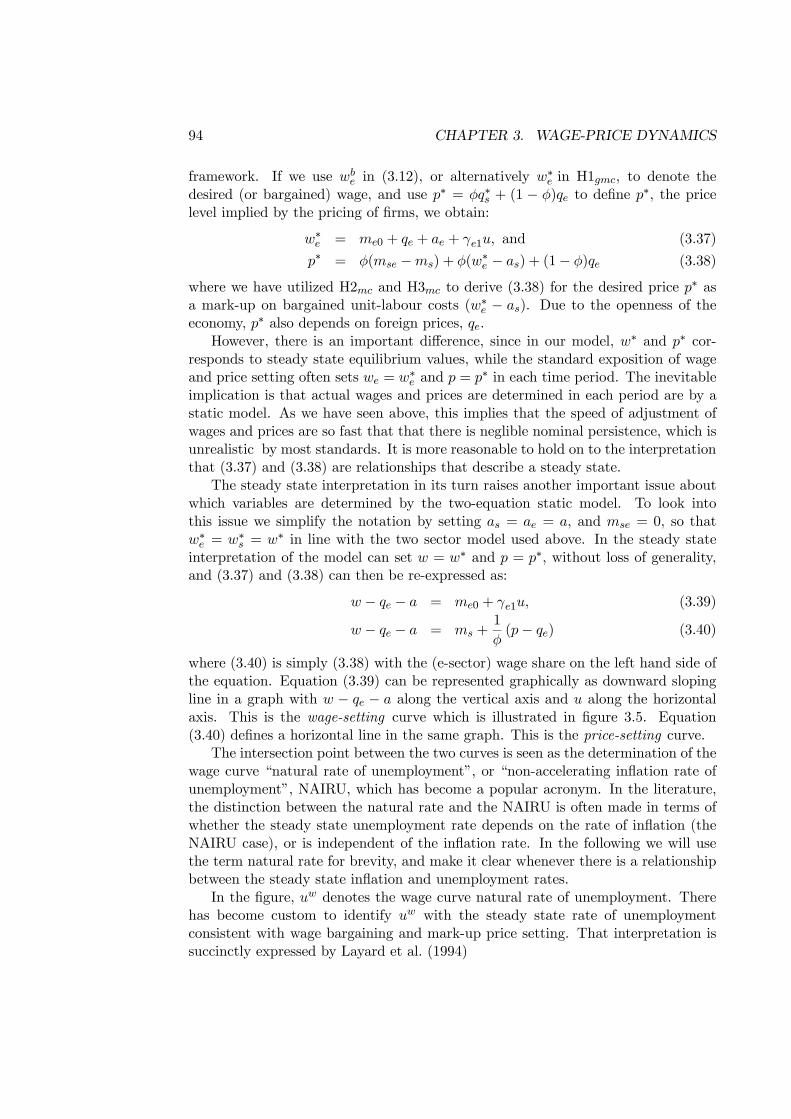
94 CHAPTER 3. WAGE-PRICE DYNAMICS
framework. If we use wbe in (3.12), or alternatively w∗e in H1gmc, to denote the
desired (or bargained) wage, and use p∗ = φq∗s + (1 − φ)qe to define p∗, the pricelevel implied by the pricing of firms, we obtain:
w∗e = me0 + qe + ae + γe1u, and (3.37)
p∗ = φ(mse −ms) + φ(w∗e − as) + (1− φ)qe (3.38)
where we have utilized H2mc and H3mc to derive (3.38) for the desired price p∗ asa mark-up on bargained unit-labour costs (w∗e − as). Due to the openness of theeconomy, p∗ also depends on foreign prices, qe.
However, there is an important difference, since in our model, w∗ and p∗ cor-responds to steady state equilibrium values, while the standard exposition of wageand price setting often sets we = w∗e and p = p∗ in each time period. The inevitableimplication is that actual wages and prices are determined in each period are by astatic model. As we have seen above, this implies that the speed of adjustment ofwages and prices are so fast that that there is neglible nominal persistence, which isunrealistic by most standards. It is more reasonable to hold on to the interpretationthat (3.37) and (3.38) are relationships that describe a steady state.
The steady state interpretation in its turn raises another important issue aboutwhich variables are determined by the two-equation static model. To look intothis issue we simplify the notation by setting as = ae = a, and mse = 0, so thatw∗e = w∗s = w∗ in line with the two sector model used above. In the steady stateinterpretation of the model can set w = w∗ and p = p∗, without loss of generality,and (3.37) and (3.38) can then be re-expressed as:
w − qe − a = me0 + γe1u, (3.39)
w − qe − a = ms +1
φ(p− qe) (3.40)
where (3.40) is simply (3.38) with the (e-sector) wage share on the left hand side ofthe equation. Equation (3.39) can be represented graphically as downward slopingline in a graph with w − qe − a along the vertical axis and u along the horizontalaxis. This is the wage-setting curve which is illustrated in figure 3.5. Equation(3.40) defines a horizontal line in the same graph. This is the price-setting curve.
The intersection point between the two curves is seen as the determination of thewage curve “natural rate of unemployment”, or “non-accelerating inflation rate ofunemployment”, NAIRU, which has become a popular acronym. In the literature,the distinction between the natural rate and the NAIRU is often made in terms ofwhether the steady state unemployment rate depends on the rate of inflation (theNAIRU case), or is independent of the inflation rate. In the following we will usethe term natural rate for brevity, and make it clear whenever there is a relationshipbetween the steady state inflation and unemployment rates.
In the figure, uw denotes the wage curve natural rate of unemployment. Therehas become custom to identify uw with the steady state rate of unemploymentconsistent with wage bargaining and mark-up price setting. That interpretation issuccinctly expressed by Layard et al. (1994)
3.2. WAGE BARGAINING AND INCOMPLETE COMPETITION. 95
Figure 3.5: Real wage and unemployment determination, NAIRU indicated by uw
.and a steady state rate of unemployment which is determined in part from outsidethe model of wage and price setting is denoted uss.
‘Only if the real wage (W/P ) desired by wage-setters is the same asthat desired by price setters will inflation be stable. And, the variablethat brings about this consistency is the level of unemployment’.18
The heuristics of this theory is that actual unemployment below the naturalrate, ut < uw, will create wage increases and expectations of future wage-priceadjustments in such a way that the result is ∆πt > 0, using the notation of section2.4.2 that πt represents the increase in the price level. Conversely, ut > uw, entailsfalling rates of inflation ∆πt < 0. uw is the only (steady state) value of ut which isconsistent with ∆πt = 0.
However, we have seen above that in the Norwegian model of inflation, there isan asymptotically stable equilibrium where both the rate of wage growth and the
18Layard et al. (1994, p 18), authors’ italics.
96 CHAPTER 3. WAGE-PRICE DYNAMICS
inflation rate are constant for any given constant rate of unemployment. Since theNorwegian model can be interpreted as a wage-bargaining model, the (emphasized)second sentence in the above quotation has been disproved already: It is not neces-sary that the steady state rate of unemployment in a bargaining model correspondsto uw in figure 3.5.19 The steady state rate of unemployment uss may be lower thanuw, as is the case shown in the graph, or higher. The figure further indicates (by a •)that the steady state wage share in general will reside at a point on the line segmentA-B: Heuristically, this is a point where price setters are trying to attain a lower realwage by nominal price increases, at the same time at the wage bargain is deliveringnominal wage increases that push real wage upwards. Hence, in the general casethe steady state is not characterized by the real wage desired by wage-setters beingthe same as that desired by price setters. Instead there is a tug-of-war equilibriumwhere the steady state real wage is a weighted average of the two parties respectivetargets for the wage share.
Bårdsen et al. (2005a, Ch 6) show which restrictions on the parameters of thedynamic equation for wage and price adjustments that are necessary for ut → uss =uw to be an implication, so that the uw corresponds to the stable steady state. Inbrief, the model must be restricted in such a way that the nominal wage and pricesetting adjustment equations become two conflicting dynamic equations for the realwage. In the context of an open economy, in particular, this step is anything buttrivial. It is not sufficient to impose a restriction referred to as dynamic homogeneityfor example (dynamic homogeneity will be defined below, in the context of thePhillips curve). What is required is n fact to purge the model of all nominal rigidity,which seems to be unrealistic on the basis of both macro and micro evidence.
We have explained that the Layard-Nickell version of the natural-rate/NAIRUconcept corresponds to a set of restrictions on the dynamic model of wage and pricesetting. As will become clear in section 3.3, a similar conclusion is true for thenatural rate of unemployment associated with a Phillips curve model for wages andprices.
The conclusion is that, special cases aside, the wage-bargaining model does notimply a unique supply-side determined steady state rate of unemployment. In orderto avoid misunderstandings, it is perhaps worth stressing that there is no contra-diction between this result, and the realistic belief that the average long-run rate ofinflation is strongly influenced by supply-side factors. The implication is only thatthe steady state rate of unemployment is left undetermined in this particular modelof the supply side. A wider iterpretation is that a realistic model of the steady statefor unemployment generally requires a richer macro model than only equations forprice and wage setting.
We end this section by noting another puzzled that has been more acknowledgedthan the problem with lack of correspondence between uw and a steady state rate of
19The exposition of wage bargaining dynamics and the Norwgian model was based on exogenousprices in the exposed sector, but this simplification represents no loss of generality regarding thisissue about the necessitry (or not) of uss = uw withing the framwork of the bargaining model.
3.2. WAGE BARGAINING AND INCOMPLETE COMPETITION. 97
unemployment. This problem is understood by noting that the price-curve dependson the relative price p − qe, so an unique intersection point in figure 3.5 does notexist unless we can fix p − qe at a certain value. Put differently: (3.39) and (3.40)are two equation in three unknown variables, and it is not clear why it is that ushould be regarded as endogenous, and not p − qe. The most used argument isthat p − qe can be regarded as determined from outside the system of wage andprice setting equations. Since p− qe is an indicator of the degree of competitivenessin the economy, it makes sense to assume that its long-run value is given by therequirement that the trade balance (or the current account) is balanced in the longterm. However, as we have seen in section 3.2.3, the properties of the dynamicwage and price setting system imply that if a steady state exists for wages (andthe wage share wt − qet − at), a steady state also exists for pt − qet. Hence, fromthis perspective there is an internal inconsistency in the approach which determinesthe steady state of the rate of unemployment from static wage and price curves, byimposing a steady-state value of p − qe from outside the model of wage and pricesetting.
3.2.8 Role of exchange rate regime
Later in the book, a main focus will be the choice of exchange rate regime, and howthat choice conditions macrodynamics. So far we have implicitly assumed that therate of foreign exchange is exogenous, corresponding to a fixed exchange rate regime.In order to make this explicit, we need to expand the notation a little. For example,the sum of the logs of productivity and foreign price
mct = aet + qet
which can be written as
mct = ∆aet +∆qet +mct−1, (3.41)
ormct = ∆aet +∆q
∗et +∆ lnEt +mct−1. (3.42)
where q∗et denotes the (log of) foreign prices in foreign currency, and Et is the nominalexchange rate (kroner/euro).20 The reason why we have suppressed the nominalexchange rate Et from the model so far, is that in a fixed exchange rate regime, theEt has no separate influence on wage growth. It does not matter whether a changein qet “comes from” a change in q∗et or in Et (a devaluation for example).
However, in the case of a floating exchange rate, we need to specify the modelof the market for foreign exchange in more detail. For example, if capital mobilityis perfect, the so called risk premium is zero and the market is characterized by
20We use the explicit notation ∆ lnEt rather than ∆et, to avoid conflict of notation with e as aidentifier of the exposed sector (for examples in subscripts).
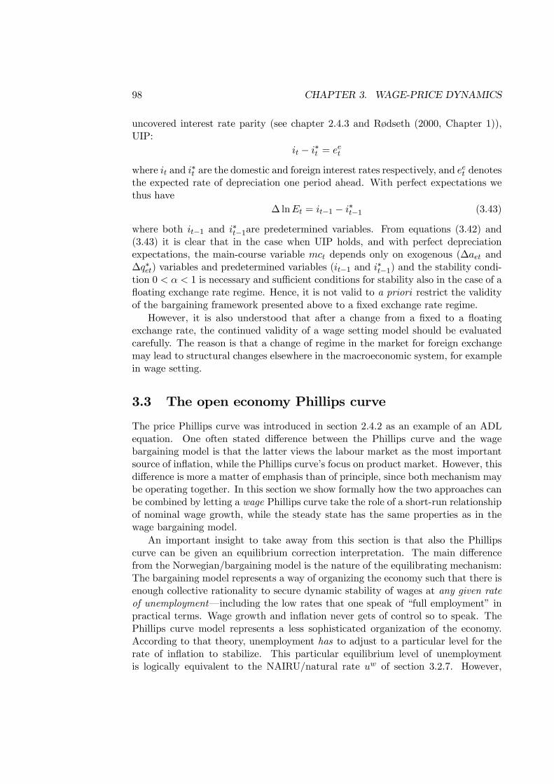
98 CHAPTER 3. WAGE-PRICE DYNAMICS
uncovered interest rate parity (see chapter 2.4.3 and Rødseth (2000, Chapter 1)),UIP:
it − i∗t = eet
where it and i∗t are the domestic and foreign interest rates respectively, and eet denotes
the expected rate of depreciation one period ahead. With perfect expectations wethus have
∆ lnEt = it−1 − i∗t−1 (3.43)
where both it−1 and i∗t−1are predetermined variables. From equations (3.42) and(3.43) it is clear that in the case when UIP holds, and with perfect depreciationexpectations, the main-course variable mct depends only on exogenous (∆aet and∆q∗et) variables and predetermined variables (it−1 and i∗t−1) and the stability condi-tion 0 < α < 1 is necessary and sufficient conditions for stability also in the case of afloating exchange rate regime. Hence, it is not valid to a priori restrict the validityof the bargaining framework presented above to a fixed exchange rate regime.
However, it is also understood that after a change from a fixed to a floatingexchange rate, the continued validity of a wage setting model should be evaluatedcarefully. The reason is that a change of regime in the market for foreign exchangemay lead to structural changes elsewhere in the macroeconomic system, for examplein wage setting.
3.3 The open economy Phillips curve
The price Phillips curve was introduced in section 2.4.2 as an example of an ADLequation. One often stated difference between the Phillips curve and the wagebargaining model is that the latter views the labour market as the most importantsource of inflation, while the Phillips curve’s focus on product market. However, thisdifference is more a matter of emphasis than of principle, since both mechanism maybe operating together. In this section we show formally how the two approaches canbe combined by letting a wage Phillips curve take the role of a short-run relationshipof nominal wage growth, while the steady state has the same properties as in thewage bargaining model.
An important insight to take away from this section is that also the Phillipscurve can be given an equilibrium correction interpretation. The main differencefrom the Norwegian/bargaining model is the nature of the equilibrating mechanism:The bargaining model represents a way of organizing the economy such that there isenough collective rationality to secure dynamic stability of wages at any given rateof unemployment–including the low rates that one speak of “full employment” inpractical terms. Wage growth and inflation never gets of control so to speak. ThePhillips curve model represents a less sophisticated organization of the economy.According to that theory, unemployment has to adjust to a particular level for therate of inflation to stabilize. This particular equilibrium level of unemploymentis logically equivalent to the NAIRU/natural rate uw of section 3.2.7. However,
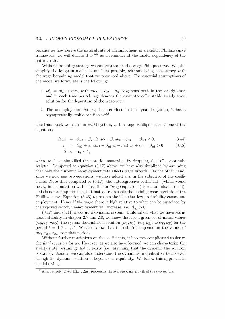
3.3. THE OPEN ECONOMY PHILLIPS CURVE 99
because we now derive the natural rate of unemployment in a explicit Phillips curveframework, we will denote it uphil as a reminder of the model dependency of thenatural rate.
Without loss of generality we concentrate on the wage Phillips curve. We alsosimplify the long-run model as much as possible, without losing consistency withthe wage bargaining model that we presented above. The essential assumptions ofthe model we formulate is the following:
1. w∗et = me0 + mct, with mct ≡ aet + qet exogenous both in the steady stateand in each time period. w∗t denotes the asymptotically stable steady statesolution for the logarithm of the wage-rate.
2. The unemployment rate ut is determined in the dynamic system, it has aasymptotically stable solution uphil.
The framework we use is an ECM system, with a wage Phillips curve as one of theequations:
∆wt = βw0 + βw1∆mct + βw2ut + εwt, βw2 < 0, (3.44)
ut = βu0 + αuut−1 + βu1(w −mc)t−1 + εut βu1 > 0 (3.45)
0 < αu < 1,
where we have simplified the notation somewhat by dropping the “e” sector sub-script.21 Compared to equation (3.17) above, we have also simplified by assumingthat only the current unemployment rate affects wage growth. On the other hand,since we now use two equations, we have added a w in the subscript of the coeffi-cients. Note that compared to (3.17), the autoregressive coefficient (which wouldbe αw in the notation with subscribt for “wage equation”) is set to unity in (3.44).This is not a simplification, but instead represents the defining characteristic of thePhillips curve. Equation (3.45) represents the idea that low profitability causes un-employment. Hence if the wage share is high relative to what can be sustained bythe exposed sector, unemployment will increase, i.e., βu1 > 0.
(3.17) and (3.44) make up a dynamic system. Building on what we have learntabout stability in chapter 2.7 and 2.8, we know that for a given set of initial values(w0,u0, mc0), the system determines a solution (w1, u1), (w2, u2), ...(wT , uT ) for theperiod t = 1, 2, ...., T . We also know that the solution depends on the values ofmct, εw t, εu,t over that period.
Without further restrictions on the coefficients, it becomes complicated to derivethe final equation for wt. However, as we also have learned, we can characterize thesteady state, assuming that it exists (i.e., assuming that the dynamic the solutionis stable). Usually, we can also understand the dynamics in qualitative terms eventhough the dynamic solution is beyond our capability. We follow this approach inthe following.
21Alternatively, given H2mc, ∆wt represents the average wage growth of the two sectors.
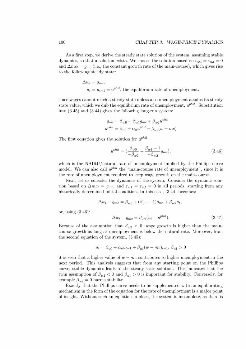
100 CHAPTER 3. WAGE-PRICE DYNAMICS
As a first step, we derive the steady state solution of the system, assuming stabledynamics, so that a solution exists. We choose the solution based on εw t = εu,t = 0and ∆mct = gmc (i.e., the constant growth rate of the main-course), which gives riseto the following steady state:
∆wt = gmc,
ut = ut−1 = uphil, the equilibrium rate of unemployment.
since wages cannot reach a steady state unless also unemployment attains its steadystate value, which we dub the equilibrium rate of unemployment, uphil. Substitutioninto (3.45) and (3.44) gives the following long-run system:
gmc = βw0 + βw1gmc + βw2uphil
uphil = βu0 + αuuphil + βu1(w −mc)
The first equation gives the solution for uphil
uphil = (βw0−βw2
+βw1 − 1−βw2
gmc), (3.46)
which is the NAIRU/natural rate of unemployment implied by the Phillips curvemodel. We can also call uphil the “main-course rate of unemployment”, since it isthe rate of unemployment required to keep wage growth on the main-course.
Next, let us consider the dynamics of the system. Consider the dynamic solu-tion based on ∆mct = gmc, and εw t = εu,t = 0 in all periods, starting from anyhistorically determined initial condition. In this case, (3.44) becomes:
∆wt − gmc = βw0 + (βw1 − 1)gmc + βw2ut,
or, using (3.46):∆wt − gmc = βw2(ut − uphil). (3.47)
Because of the assumption that βw2 < 0, wage growth is higher than the main-course growth as long as unemployment is below the natural rate. Moreover, fromthe second equation of the system, (3.45):
ut = βu0 + αuut−1 + βu1(w −mc)t−1, βu1 > 0
it is seen that a higher value of w −mc contributes to higher unemployment in thenext period. This analysis suggests that from any starting point on the Phillipscurve, stable dynamics leads to the steady state solution. This indicates that thetwin assumption of βw2 < 0 and βu1 > 0 is important for stability. Conversely, forexample βw2 = 0 harms stability.
Exactly that the Phillips curve needs to be supplemented with an equilibratingmechanism in the form of the equation for the rate of unemployment is a major pointof insight. Without such an equation in place, the system is incomplete, as there is
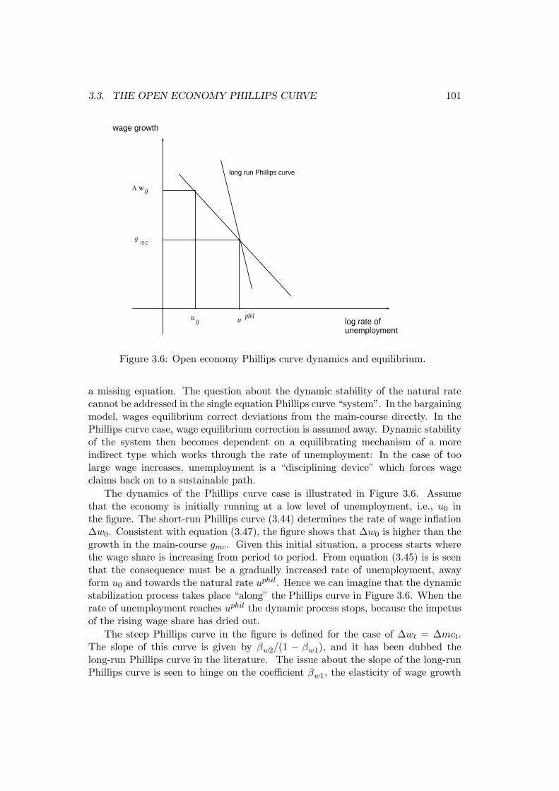
3.3. THE OPEN ECONOMY PHILLIPS CURVE 101
wage growth
g mc
philuu0 log rate of
unemployment
long run Phillips curve
Δ w 0
Figure 3.6: Open economy Phillips curve dynamics and equilibrium.
a missing equation. The question about the dynamic stability of the natural ratecannot be addressed in the single equation Phillips curve “system”. In the bargainingmodel, wages equilibrium correct deviations from the main-course directly. In thePhillips curve case, wage equilibrium correction is assumed away. Dynamic stabilityof the system then becomes dependent on a equilibrating mechanism of a moreindirect type which works through the rate of unemployment: In the case of toolarge wage increases, unemployment is a “disciplining device” which forces wageclaims back on to a sustainable path.
The dynamics of the Phillips curve case is illustrated in Figure 3.6. Assumethat the economy is initially running at a low level of unemployment, i.e., u0 inthe figure. The short-run Phillips curve (3.44) determines the rate of wage inflation∆w0. Consistent with equation (3.47), the figure shows that ∆w0 is higher than thegrowth in the main-course gmc. Given this initial situation, a process starts wherethe wage share is increasing from period to period. From equation (3.45) is is seenthat the consequence must be a gradually increased rate of unemployment, awayform u0 and towards the natural rate uphil. Hence we can imagine that the dynamicstabilization process takes place “along” the Phillips curve in Figure 3.6. When therate of unemployment reaches uphil the dynamic process stops, because the impetusof the rising wage share has dried out.
The steep Phillips curve in the figure is defined for the case of ∆wt = ∆mct.The slope of this curve is given by βw2/(1 − βw1), and it has been dubbed thelong-run Phillips curve in the literature. The issue about the slope of the long-runPhillips curve is seen to hinge on the coefficient βw1, the elasticity of wage growth
102 CHAPTER 3. WAGE-PRICE DYNAMICS
with respect to the growth in the main-course. In the figure, the long-run curveis downward sloping, corresponding to βw1 < 1 which is referred to as dynamicinhomogeneity in wage setting. The converse, referred to as dynamic homogeneityin the literature, implies βw1 = 1, and the long-run Phillips curve is then vertical.Subject to dynamic homogeneity, the equilibrium rate uphil is independent of worldinflation and productivity growth gmc.
3.3. THE OPEN ECONOMY PHILLIPS CURVE 103
Box 3.1 (A “bargaining based Phillips curve”?) Some im-portant textbooks, for example Burda and Wyplosz (2005, Chapter12.3) give a different message from ours, namely that wage bar-gaining gives raise to a standard price Phillips curve. However,that argument takes too lightly on the distinction between staticrelationships and dynamic adjustment. To show how, consider aclosed economy version of our static model. Wage bargaining is thenfor the whole economy so we replace equation (3.12) by:
w∗ = m0 + p∗ + a+ γ1u, γ1 < 0 (3.48)
and, the steady state price equation is simply.
p∗ = ln( ) + w∗ − a, > 1. (3.49)
Burda and Wyplosz then set w∗ = w in both equations. However, inthe wage equation p∗ is replaced by pe which denotes the expected pricelevel, while in the price equation p∗ = p. Finally, time subscripts areadded in both equations to give
wt − at = m0t + pet + γ1ut, and
wt − at = − ln( t) + pt.
Solving for pt gives
pt = ln( t) +m0t + pet + γ1ut,
and taking the difference on both sides of the equation gives:
∆πt = ∆(ln( t) +m0t) +∆πet + γ1∆ut. (3.50)
Equation (3.50) is identical to Burda and Wyplosz’s equation (12.11),with small qualification that they (implicitly) set ∆ut = 0. Their“bargaining” Phillips curve also assumes
∆(− ln( t) +m0t) = a(Yt − Y ).
where Yt is GDP and Y the full employment output, in other wordsthe output-gap (which is seen as perfectly correlated with the differ-ence between current unemployment and the natural rate).
104 CHAPTER 3. WAGE-PRICE DYNAMICS
The slope of the long-run Phillips curve represented one of the most debatedissues in macroeconomics in the 1970 and 1980s. One arguments in favour of avertical long-run Phillips curve is that workers are able to obtain full compensationfor price increases. Therefore, in the context of our model, βw1 = 1 is perhapsthe the only reasonable parameter value. The downward sloping long-run Phillipscurve has also been denounced on the grounds that it gives a too optimistic pictureof the powers of economic policy: namely that the government can permanentlyreduce the level of unemployment below the natural rate by “fixing” a suitablyhigh level of inflation, see e.g., Romer (1996, Ch 5.5). In the context of an openeconomy this discussion appears as somewhat exaggerated, since a long-run trade-offbetween inflation and unemployment in any case does not follow from the premiseof a downward-sloping long-run curve. Instead, as shown in figure 3.6, the steadystate level of unemployment is determined by the rate of imported inflation andproductivity growth as represented by gmc. Neither of these are instruments ofeconomic policy.22
Both the wage Phillips curve of this section, and the model for wages in section3.2.4 have been kept deliberately simple. In the real economy, cost-of-living con-siderations play a significant role in wage setting. Thus, in empirical models oneusually includes current and lagged consumer price inflation in the wage equation.Section 3.5 shows an empirical example. The above formal framework above canextended to accommodate this, without changing the conclusion about the steadystate solution.
Another important factor which we have omitted so far from the formal analysis,is expectations. For example, instead of (3.44) we might have
∆wt = βw0 + βw1∆wet + βw2ut + εwt,
or ∆wet+1 for that matter. However, as long as expectations are influenced by the
main-course variable, we will retrieve the same conclusion as above. For example
∆wet = ϕ∆mct + (1− ϕ)∆wt−1, 0 < ϕ ≤ 1
In a steady state there are no expectations errors, so
∆wet = ∆wt−1 = gmc
as before.In section 3.2.3 we showed the implications of the bargaining model for domestic
inflation. To establish the corresponding result for the case of the Phillips curvemodel, we repeat the definitional equation for the consumer price index:
pt = φqst + (1− φ)qet, 0 < φ < 1,
or, in differences∆pt = φ∆qst + (1− φ)∆qet. (3.51)
22To affect uphil, policy needs to incur a higher or lower permanent rate of currency depreciation.

3.4. SUMMINGUP THENORWEGAINMODELOF INFLATIONANDTHE PHILLIPS CURVEMODE
Using the same simplifying assumptions as in section 3.2.3, for example that shel-tered sector price growth is always on the long-run equilibrium path implied by themain-course theory, we obtain the price Phillips curve:
∆pt = φβw0 + {φβw1 + (1− φ)}∆qet + φβw2ut + φβw1∆aet − φ∆ast + φεwt. (3.52)
Hence, the reduced form inflation equation contains basically the same explana-tory variables as the bargaining model. The exception is the absence of the wageequilibrium correction term.
Equation (3.52) is the counterpart to the standard price Phillips curve foundin all current textbooks, for example Blanchard (2005, Ch 8). Without any logicalinconsistencies, the Phillips curve can be augmented with terms that represent ex-pectations, which can originate in wage setting (as hinted immediately above), orin s-sector price setting. As long as these expectation are based on experience, theywill (only) imply a more complicated dynamic structure, but they will not affect theessential model properties that we have focused on in this section.
3.4 Summing up the Norwegain model of inflation andthe Phillips curve model
So far in this chapter we have presented two dynamic models of wage setting. Bothare much used in modern macroeconomic thinking and model building. The follow-ing 7 points summarize the main results.
1. The first model used bargaining theory to rationalize a long run relationshipbetween the wage level of the exposed sector and its main determinants: Prod-uct price (qet), productivity (aet) and the rate of unemployment (ut). The elas-ticities of product price and productivity are both unity, and we therefore oftensubsume these two variables in one variable mct = qet + aet. With referenceto an earlier theoretical development, the variable is called the main-coursevariable since it defines a long-run trend followed by wages.
2. If the long run wage equation is to correspond to a stable steady state growthpath, we showed that there has to be a stable ADL equation for wages (i.e.,0 < α < 1,in the equation for wet), which can be transformed into an ECMfor wage growth.
3. The dynamic properties of the wage bargaining model are:
(a) For a given (exogenously determined) level of ut,wage growth equilibrium-corrects deviations form the main-course.
(b) Therefore, there is a steady state level for the logarith omf ware share(wet −mct).
106 CHAPTER 3. WAGE-PRICE DYNAMICS
(c) Stability of wage growth and inflation also follows, even without assump-tions about further equilibrium correcting behaviour in s-sector wage set-ting, or in price formation.
4. The second model postulates a wage Phillips curve, PCM, consistent withsetting α = 1 in the wage ADL equation. The following results were found tohold for the PCM specification of wage dynamics.
(a) The PCM (by itself, viewed isolated from the rest of the model economy)gives an unstable solution for the wage share wet −mct.
(b) If the PCM is linked up with a second equation, which explains ut as anincreasing function of the wage share, the two equation system implies asteady state level for the ware share wet −mct.
(c) The PCM implies a natural rate of unemployment (uphil) which cor-responds to the steady state level of unemployment implied by the 2-equation system.
5. Hence both models (wage bargaining and the PCM) implies a asymtoticallystable wage share, and also stable rates of wage and price inflation.
6. The difference between the models lies in the mechanism that secures stabilityof the wage share
(a) In the wage brgainig case tere is an amount of collective rationality. Forexample: Unions adjust their wage claims to the last years profitability.Inflation is stabilized at any given rate of unemployment, also low onesthat prevailed in Europe until 1980 and in Scandinavia until the end oflast century.
(b) In the PCM case: There is less collective rationality. Instead unemploy-ment serves as a disciplining device: There is only one level of unem-ployment at which the rate of inflation is stable, i.e., the natural rate ofunemployment.
7. There seems to be some important implications for policy. For example:
(a) If PCM is the true model, then self-defeating policy to try to target “fullunemployment” below the natural rate.
(b) If the wage bargaing moodel is the true model then it is not only pos-sible to target full unemployment, it may also be advisable in order tomaintain collective rationality (avoid breakdown in the bargaining sys-tem/institutions).
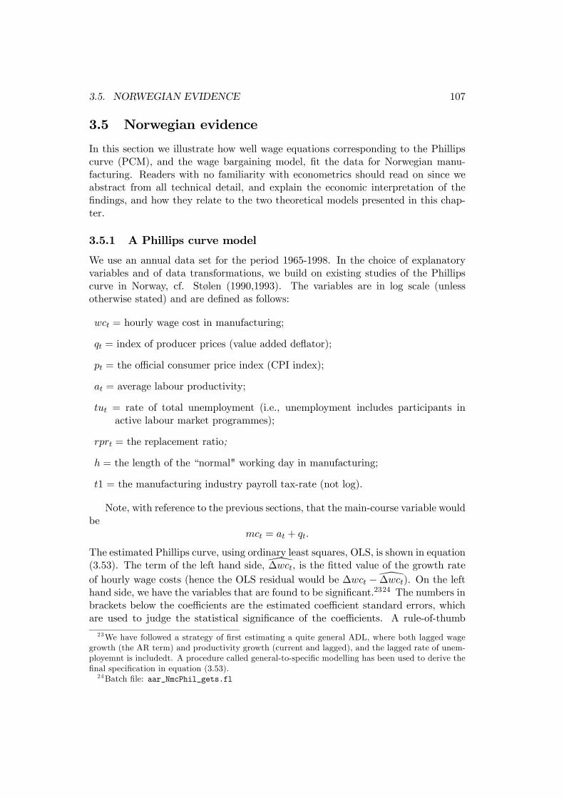
3.5. NORWEGIAN EVIDENCE 107
3.5 Norwegian evidence
In this section we illustrate how well wage equations corresponding to the Phillipscurve (PCM), and the wage bargaining model, fit the data for Norwegian manu-facturing. Readers with no familiarity with econometrics should read on since weabstract from all technical detail, and explain the economic interpretation of thefindings, and how they relate to the two theoretical models presented in this chap-ter.
3.5.1 A Phillips curve model
We use an annual data set for the period 1965-1998. In the choice of explanatoryvariables and of data transformations, we build on existing studies of the Phillipscurve in Norway, cf. Stølen (1990,1993). The variables are in log scale (unlessotherwise stated) and are defined as follows:
wct = hourly wage cost in manufacturing;
qt = index of producer prices (value added deflator);
pt = the official consumer price index (CPI index);
at = average labour productivity;
tut = rate of total unemployment (i.e., unemployment includes participants inactive labour market programmes);
rprt = the replacement ratio;
h = the length of the “normal" working day in manufacturing;
t1 = the manufacturing industry payroll tax-rate (not log).
Note, with reference to the previous sections, that the main-course variable wouldbe
mct = at + qt.
The estimated Phillips curve, using ordinary least squares, OLS, is shown in equation(3.53). The term of the left hand side,\∆wct, is the fitted value of the growth rateof hourly wage costs (hence the OLS residual would be ∆wct −\∆wct). On the lefthand side, we have the variables that are found to be significant.2324 The numbers inbrackets below the coefficients are the estimated coefficient standard errors, whichare used to judge the statistical significance of the coefficients. A rule-of-thumb
23We have followed a strategy of first estimating a quite general ADL, where both lagged wagegrowth (the AR term) and productivity growth (current and lagged), and the lagged rate of unem-ployemnt is includedt. A procedure called general-to-specific modelling has been used to derive thefinal specification in equation (3.53).24Batch file: aar_NmcPhil_gets.fl
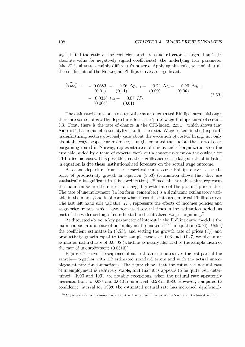
108 CHAPTER 3. WAGE-PRICE DYNAMICS
says that if the ratio of the coefficient and its standard error is larger than 2 (inabsolute value for negatively signed coefficients), the underlying true parameter(the β) is almost certainly different from zero. Applying this rule, we find that allthe coefficients of the Norwegian Phillips curve are significant.
\∆wct = − 0.0683(0.01)
+ 0.26(0.11)
∆pt−1 + 0.20(0.09)
∆qt + 0.29(0.06)
∆qt−1
− 0.0316(0.004)
tut − 0.07(0.01)
IPt(3.53)
The estimated equation is recognizable as an augmented Phillips curve, althoughthere are some noteworthy departures form the ‘pure’ wage Phillips curve of section3.3. First, there is the rate of change in the CPI-index, ∆pt−1, which shows thatAukrust’s basic model is too stylized to fit the data. Wage setters in the (exposed)manufacturing sectors obviously care about the evolution of cost-of living, not onlyabout the wage-scope For reference, it might be noted that before the start of eachbargaining round in Norway, representatives of unions and of organizations on thefirm side, aided by a team of experts, work out a consensus view on the outlook forCPI price increases. It is possible that the significance of the lagged rate of inflationin equation is due these institutionalized forecasts on the actual wage outcome.
A second departure from the theoretical main-course Phillips curve is the ab-sence of productivity growth in equation (3.53) (estimation shows that they arestatistically insignificant in this specification). Hence, the variables that representthe main-course are the current an lagged growth rate of the product price index.The rate of unemployment (in log form, remember) is a significant explanatory vari-able in the model, and is of course what turns this into an empirical Phillips curve.The last left hand side variable, IPt, represents the effects of incomes policies andwage-price freezes, which have been used several times in the estimation period, aspart of the wider setting of coordinated and centralized wage bargaining.25
As discussed above, a key parameter of interest in the Phillips curve model is themain-course natural rate of unemployment, denoted uphil in equation (3.46). Usingthe coefficient estimates in (3.53), and setting the growth rate of prices (δf ) andproductivity growth equal to their sample means of 0.06 and 0.027, we obtain anestimated natural rate of 0.0305 (which is as nearly identical to the sample mean ofthe rate of unemployment (0.0313)).
Figure 3.7 shows the sequence of natural rate estimates over the last part of thesample– together with ±2 estimated standard errors and with the actual unem-ployment rate for comparison. The figure shows that the estimated natural rateof unemployment is relatively stable, and that it is appears to be quite well deter-mined. 1990 and 1991 are notable exceptions, when the natural rate apparentlyincreased from to 0.033 and 0.040 from a level 0.028 in 1989. However, compared toconfidence interval for 1989, the estimated natural rate has increased significantly25IPt is a so called dummy variable: it is 1 when incomes policy is ‘on’, and 0 whne it is ‘off ’.
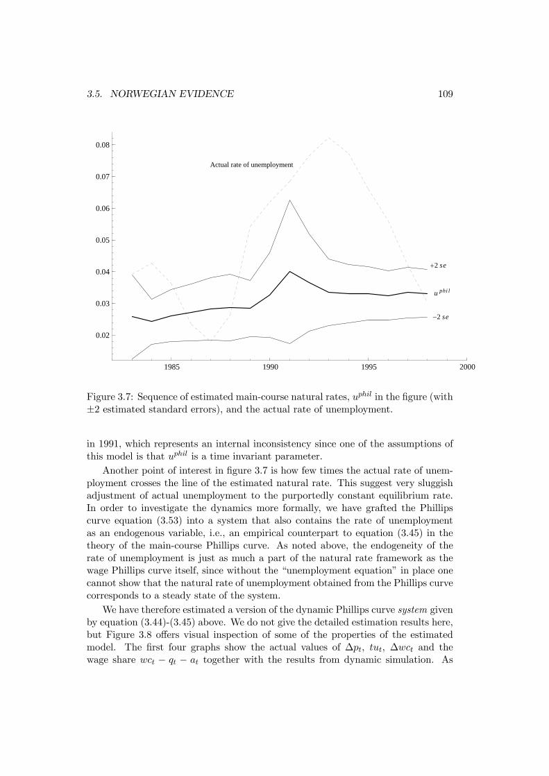
3.5. NORWEGIAN EVIDENCE 109
1985 1990 1995 2000
0.02
0.03
0.04
0.05
0.06
0.07
0.08
u phi l
+2 se
−2 se
Actual rate of unemployment
Figure 3.7: Sequence of estimated main-course natural rates, uphil in the figure (with±2 estimated standard errors), and the actual rate of unemployment.
in 1991, which represents an internal inconsistency since one of the assumptions ofthis model is that uphil is a time invariant parameter.
Another point of interest in figure 3.7 is how few times the actual rate of unem-ployment crosses the line of the estimated natural rate. This suggest very sluggishadjustment of actual unemployment to the purportedly constant equilibrium rate.In order to investigate the dynamics more formally, we have grafted the Phillipscurve equation (3.53) into a system that also contains the rate of unemploymentas an endogenous variable, i.e., an empirical counterpart to equation (3.45) in thetheory of the main-course Phillips curve. As noted above, the endogeneity of therate of unemployment is just as much a part of the natural rate framework as thewage Phillips curve itself, since without the “unemployment equation” in place onecannot show that the natural rate of unemployment obtained from the Phillips curvecorresponds to a steady state of the system.
We have therefore estimated a version of the dynamic Phillips curve system givenby equation (3.44)-(3.45) above. We do not give the detailed estimation results here,but Figure 3.8 offers visual inspection of some of the properties of the estimatedmodel. The first four graphs show the actual values of ∆pt, tut, ∆wct and thewage share wct − qt − at together with the results from dynamic simulation. As
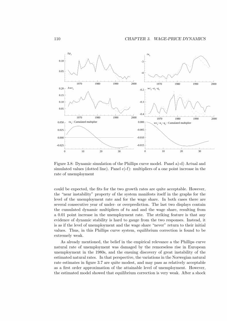
110 CHAPTER 3. WAGE-PRICE DYNAMICS
1970 1980 1990 2000
0.05
0.10
Δpt
1970 1980 1990 2000
-4
-3
tut
1970 1980 1990 2000
0.05
0.10
0.15
0.20 Δwct
1970 1980 1990 2000
-0.4
-0.3
-0.2 wct−at−qt
0 10 20 30
-0.025
0.000
0.025
0.050 tut : Cumulated multiplier
0 10 20 30
-0.015
-0.010
-0.005
0.000 wct−at−qt : Cumulated multiplier
Figure 3.8: Dynamic simulation of the Phillips curve model. Panel a)-d) Actual andsimulated values (dotted line). Panel e)-f): multipliers of a one point increase in therate of unemployment
could be expected, the fits for the two growth rates are quite acceptable. However,the “near instability” property of the system manifests itself in the graphs for thelevel of the unemployment rate and for the wage share. In both cases there areseveral consecutive year of under- or overprediction. The last two displays containthe cumulated dynamic multipliers of tu and and the wage share, resulting froma 0.01 point increase in the unemployment rate. The striking feature is that anyevidence of dynamic stability is hard to gauge from the two responses. Instead, itis as if the level of unemployment and the wage share “never” return to their initialvalues. Thus, in this Phillips curve system, equilibrium correction is found to beextremely weak.
As already mentioned, the belief in the empirical relevance a the Phillips curvenatural rate of unemployment was damaged by the remorseless rise in Europeanunemployment in the 1980s, and the ensuing discovery of great instability of theestimated natural rates. In that perspective, the variations in the Norwegian naturalrate estimates in figure 3.7 are quite modest, and may pass as relatively acceptableas a first order approximation of the attainable level of unemployment. However,the estimated model showed that equilibrium correction is very weak. After a shock
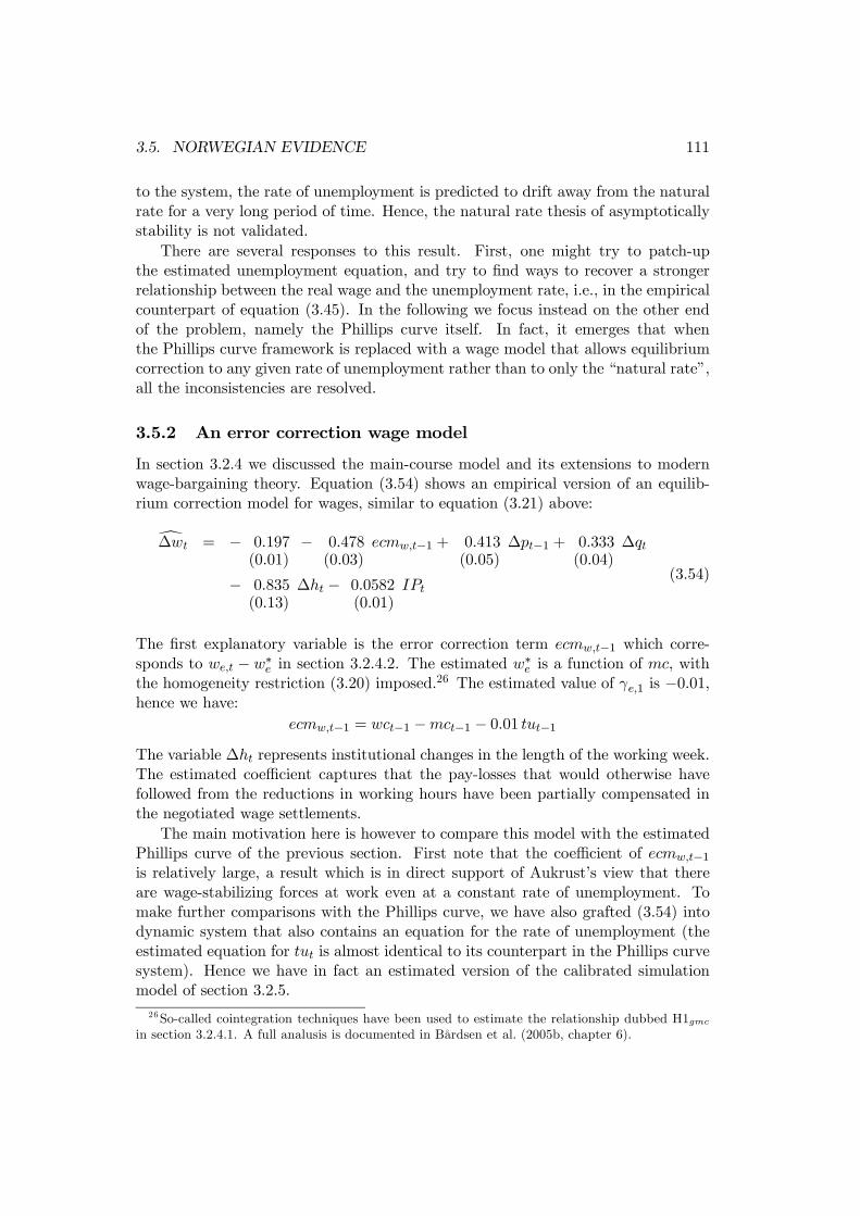
3.5. NORWEGIAN EVIDENCE 111
to the system, the rate of unemployment is predicted to drift away from the naturalrate for a very long period of time. Hence, the natural rate thesis of asymptoticallystability is not validated.
There are several responses to this result. First, one might try to patch-upthe estimated unemployment equation, and try to find ways to recover a strongerrelationship between the real wage and the unemployment rate, i.e., in the empiricalcounterpart of equation (3.45). In the following we focus instead on the other endof the problem, namely the Phillips curve itself. In fact, it emerges that whenthe Phillips curve framework is replaced with a wage model that allows equilibriumcorrection to any given rate of unemployment rather than to only the “natural rate”,all the inconsistencies are resolved.
3.5.2 An error correction wage model
In section 3.2.4 we discussed the main-course model and its extensions to modernwage-bargaining theory. Equation (3.54) shows an empirical version of an equilib-rium correction model for wages, similar to equation (3.21) above:
d∆wt = − 0.197(0.01)
− 0.478(0.03)
ecmw,t−1 + 0.413(0.05)
∆pt−1 + 0.333(0.04)
∆qt
− 0.835(0.13)
∆ht − 0.0582(0.01)
IPt(3.54)
The first explanatory variable is the error correction term ecmw,t−1 which corre-sponds to we,t − w∗e in section 3.2.4.2. The estimated w∗e is a function of mc, withthe homogeneity restriction (3.20) imposed.26 The estimated value of γe,1 is −0.01,hence we have:
ecmw,t−1 = wct−1 −mct−1 − 0.01 tut−1The variable ∆ht represents institutional changes in the length of the working week.The estimated coefficient captures that the pay-losses that would otherwise havefollowed from the reductions in working hours have been partially compensated inthe negotiated wage settlements.
The main motivation here is however to compare this model with the estimatedPhillips curve of the previous section. First note that the coefficient of ecmw,t−1is relatively large, a result which is in direct support of Aukrust’s view that thereare wage-stabilizing forces at work even at a constant rate of unemployment. Tomake further comparisons with the Phillips curve, we have also grafted (3.54) intodynamic system that also contains an equation for the rate of unemployment (theestimated equation for tut is almost identical to its counterpart in the Phillips curvesystem). Hence we have in fact an estimated version of the calibrated simulationmodel of section 3.2.5.26So-called cointegration techniques have been used to estimate the relationship dubbed H1gmc
in section 3.2.4.1. A full analusis is documented in Bårdsen et al. (2005b, chapter 6).
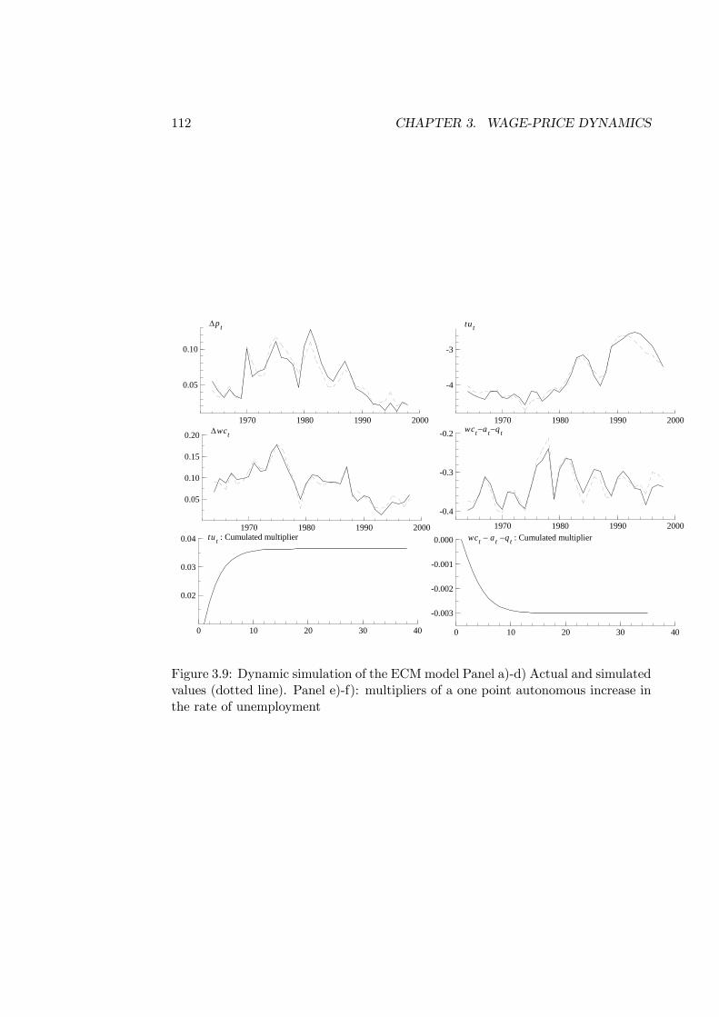
112 CHAPTER 3. WAGE-PRICE DYNAMICS
1970 1980 1990 2000
0.05
0.10
0.15
0.20 Δwct
1970 1980 1990 2000
0.05
0.10
Δpt
1970 1980 1990 2000
-4
-3
tut
0 10 20 30 40
0.02
0.03
0.04 tut : Cumulated multiplier
0 10 20 30 40
-0.003
-0.002
-0.001
0.000 wct − at −qt : Cumulated multiplier1970 1980 1990 2000
-0.4
-0.3
-0.2 wct−at−qt
Figure 3.9: Dynamic simulation of the ECMmodel Panel a)-d) Actual and simulatedvalues (dotted line). Panel e)-f): multipliers of a one point autonomous increase inthe rate of unemployment
3.6. THE NEW KEYNESIAN PHILLIPS CURVE 113
Some properties of that system is illustrated in figure 3.9. For each of the fourendogenous variables shown in the figure, the model solution (i.e. the lines denoted“simulated values”) is closer to the actual value than is the case in Figure 3.8 forthe Phillips curve system. The two last panels in the figure show the cumulateddynamic multiplier of an exogenous shock to the rate of unemployment. The dif-ference from figure 3.8, where the steady state was not even “in sight” within the35 year simulation period, are striking. In figure 3.9, 80% of the long-run effect isreached within 4 years, and the system has reached a new steady state by the end ofthe first 10 years of the solution period. The conclusion is that this system is moreconvincingly stable than the Phillips curve version of the main-course model. Notealso that the estimated model, which uses real data of the Norwegian economy, hasthe same dynamic properties as the calibrated theory model of section 3.2.5.
Economists are known to state that it is necessary to assume a vertical Phillipscurve to ensure dynamic stability of the macroeconomy. In opposition to this view,the evidence presented here shows not only that the wage price system is stablewhen the Phillips curve is substituted by a wage equation which incorporates directadjustment also with respect to profitability (consistent with the Norwegian modeland with modern bargaining theory). Quite plainly, the system with the alternative(equilibrium correcting) wage equation has much more convincing stability proper-ties than the Phillips curve system.
3.6 The New Keynesian Phillips curve
The New Keynesian Phillips Curve, NPC hereafter, has rapidly gained popularityand has become an integral part of the New Keynesian Model of monetary policy,as the aggregate supply equation in that model.
Compared to the models above which addressed wage and price setting jointly,the theory of the NPC is one-sided it its focus on firms’ price setting. Although thismay seem to be a drawback, it nevertheless explains some of the success of the NPC.The omission of a theory of trade union behaviour for example makes the NPC fitlike hand in glove into dynamic stochastic equilibrium models (DSGE models) whichassumes that the labour market is perfectly competitive, and that each individualchooses her own wage in an optimal way. Unemployment is not recognized as aneconomic pathology, fluctuations on hours worked being instead interpreted as dueto intertemporal substitution of labour.27 In this respect DSGE models are similarto the RBC model in chapter 2.8.4.
3.6.1 The ‘pure’ NPC model
Galí and Gertler (1999) gives a formulation of the NPC which is in line with themodel by Calvo (1983) on staggered contracts and rational expectations: Theyassume that a representative firm takes account of the expected future path of
27The seminal presentation of the DSGE framework is the paper by Smets and Wouters (2003).
114 CHAPTER 3. WAGE-PRICE DYNAMICS
nominal marginal costs when setting its price, given a probability that the pricethus set “today” will remain fixed for many time periods ahead. This leads to a anequation of the form
∆pt = bp1Et∆pt+1 + bp2xt + εpt, bp1 > 0, bp2 ≥ 0, (3.55)
where pt denotes the logarithm of a general price index. Note that we make a slightchange in the notation that we have used above, where we distinguished betweenproduct prices in the two sectors of the open economy, and pt denoted the consumerprice index of the open economy.
Et∆pt+1 denotes expected inflation one period ahead conditional upon informa-tion available at time t. As you may have become accustomed to by now, εpt in(3.55) denotes a disturbance term. In the NPC in (3.55), xt denotes the logarithmof the wage share, which Gali and Gertler argue is the best operational measure ofthe firm’s real marginal costs which is the theoretical explanatory variable. Withthis definition of xt in mind, note that (3.55) can be written as
pt =1
1 + bp2(pt−1 + bp1Et∆pt+1) +
bp21 + bp2
(wt − at) + εpt
which takes the same general form as the static normal cost pricing model, forexample equation (3.15), but the mark-up coefficient is variable in the NPC model,and the elasticity with respect to the unit labour costs is less than one.
Although Gali and Gertler prefer the wage-share formulation, it might be notedthat Roberts (1995) has shown that several New Keynesian models have (3.55) asa common representation, but with different operational measures of xt. Hence, inthe bigger picture, equations using the output gap, the unemployment rate or thewage share in logs, can all be counted as NPC models of inflation. It is understoodthat when the unemployment rate is used, bp2 ≤ 0.
The rationale for the forward-looking term in (3.55) is the assumption of stag-gered price setting. As mentioned, the assumption is that each price setter knowsthat with a high probability, her next opportunity to adjust the price of her firm’sproduct lies several periods into the future. Hence it is optimal to take the expectedprice changes of other price setters into account. When everybody behaves in thisway at the micro level, the macro outcome is the functional relationship given inequation (3.55), between the expected rate of change in the price level one periodahead, and today’s rate of inflation.
The appearance of the forward-looking term Et∆pt+1 has important consequencesfor the dynamic stability properties of this model of inflation. To understandhow, replace the expectations term with the actual forward rate, using Et∆pt+1 =∆pt+1 − ηt+1, where ηt+1 is the expectations error, to obtain
∆pt = bp1∆pt+1 + bp2xt + p,t (3.56)
where p,t = εpt− bp1ηt+1 is the joint disturbance term made up of the expectationserror and the inflation surprise term εpt. This equation is very much like an ADL
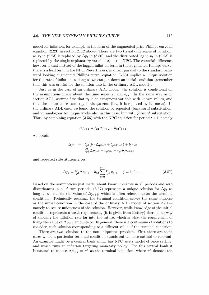
3.6. THE NEW KEYNESIAN PHILLIPS CURVE 115
model for inflation, for example in the form of the augmented price Phillips curve inequation (2.23) in section 2.4.2 above. There are two trivial differences of notation:as πt in (2.23) is replaced by ∆pt in (3.56), and the distributed lag in ut in (2.23) isreplaced by the single explanatory variable xt in the NPC. The essential differencehowever is that instead of the lagged inflation term in the augmented Phillips curve,there is a lead term in the NPC. Nevertheless, in direct parallel to the standard back-ward looking augmented Phillips curve, equation (3.56) implies a unique solutionfor the rate of inflation, as long as we can pin down an initial condition (rememberthat this was crucial for the solution also in the ordinary ADL model).
Just as in the case of an ordinary ADL model, the solution is conditional onthe assumptions made about the time series xt and p,t. In the same way as insection 2.7.1, assume first that xt is an exogenous variable with known values, andthat the disturbance term p,t is always zero (i.e., it is replaced by its mean). Inthe ordinary ADL case, we found the solution by repeated (backward) substitution,and an analogous technique works also in this case, but with forward substitution.Thus, by combining equation (3.56) with the NPC equation for period t+1, namely
∆pt+1 = bp1∆pt+2 + bp2xt+1
we obtain
∆pt = bp1(bp1∆pt+2 + bp2xt+1) + bp2xt
= b2p1∆pt+2 + bp2xt + bp1bp2xt+1
and repeated substitution gives
∆pt = bjp1∆pt+j + bp2
j−1Xi=0
bip1xt+i, j = 1, 2, ..... (3.57)
Based on the assumptions just made, about known x-values in all periods and zerodisturbances in all future periods, (3.57) represents a unique solution for ∆pt aslong as we can fix the value of ∆pt+j , which is often referred to as the terminalcondition. Technically peaking, the terminal condition serves the same purposeas the initial condition in the case of the ordinary ADL model of section 2.7.1–namely to secure uniqueness of the solution. However, while knowledge of the initialcondition represents a weak requirement, (it is given from history) there is no wayof knowing the inflation rate far into the future, which is what the requirement offixing the value of ∆pt+j amounts to. In general, there is a continuum of solutions toconsider, each solution corresponding to a different value of the terminal condition.
There are two solutions to the non-uniqueness problem. First there are somecases where a particular terminal condition stands out as more natural or relevant.An example might be a central bank which has NPC as its model of price setting,and which runs an inflation targeting monetary policy. For this central bank itis natural to choose ∆pt+j = π∗ as the terminal condition, where π∗ denotes the
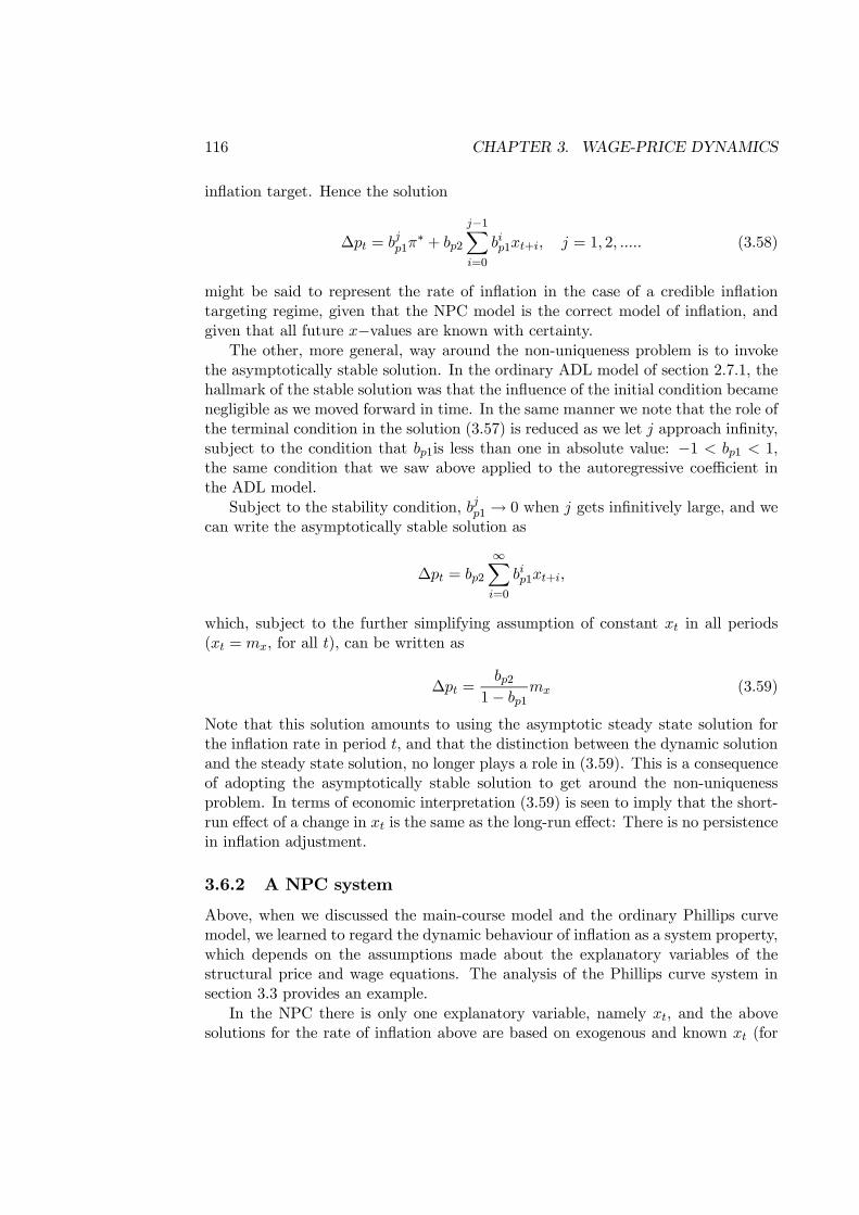
116 CHAPTER 3. WAGE-PRICE DYNAMICS
inflation target. Hence the solution
∆pt = bjp1π∗ + bp2
j−1Xi=0
bip1xt+i, j = 1, 2, ..... (3.58)
might be said to represent the rate of inflation in the case of a credible inflationtargeting regime, given that the NPC model is the correct model of inflation, andgiven that all future x−values are known with certainty.
The other, more general, way around the non-uniqueness problem is to invokethe asymptotically stable solution. In the ordinary ADL model of section 2.7.1, thehallmark of the stable solution was that the influence of the initial condition becamenegligible as we moved forward in time. In the same manner we note that the role ofthe terminal condition in the solution (3.57) is reduced as we let j approach infinity,subject to the condition that bp1is less than one in absolute value: −1 < bp1 < 1,the same condition that we saw above applied to the autoregressive coefficient inthe ADL model.
Subject to the stability condition, bjp1 → 0 when j gets infinitively large, and wecan write the asymptotically stable solution as
∆pt = bp2
∞Xi=0
bip1xt+i,
which, subject to the further simplifying assumption of constant xt in all periods(xt = mx, for all t), can be written as
∆pt =bp2
1− bp1mx (3.59)
Note that this solution amounts to using the asymptotic steady state solution forthe inflation rate in period t, and that the distinction between the dynamic solutionand the steady state solution, no longer plays a role in (3.59). This is a consequenceof adopting the asymptotically stable solution to get around the non-uniquenessproblem. In terms of economic interpretation (3.59) is seen to imply that the short-run effect of a change in xt is the same as the long-run effect: There is no persistencein inflation adjustment.
3.6.2 A NPC system
Above, when we discussed the main-course model and the ordinary Phillips curvemodel, we learned to regard the dynamic behaviour of inflation as a system property,which depends on the assumptions made about the explanatory variables of thestructural price and wage equations. The analysis of the Phillips curve system insection 3.3 provides an example.
In the NPC there is only one explanatory variable, namely xt, and the abovesolutions for the rate of inflation above are based on exogenous and known xt (for
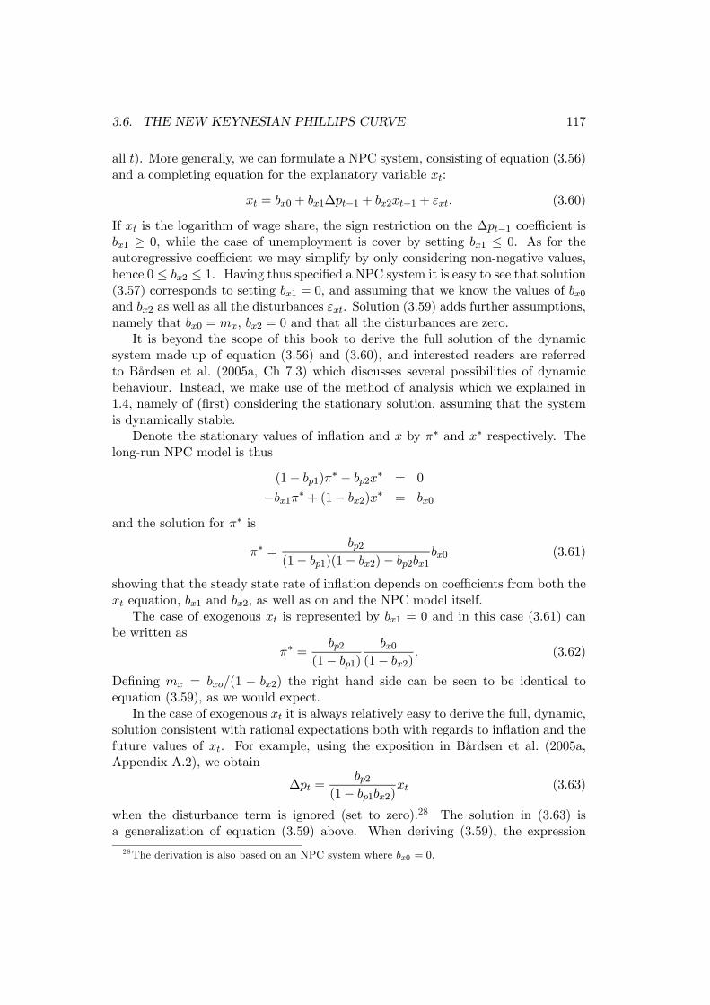
3.6. THE NEW KEYNESIAN PHILLIPS CURVE 117
all t). More generally, we can formulate a NPC system, consisting of equation (3.56)and a completing equation for the explanatory variable xt:
xt = bx0 + bx1∆pt−1 + bx2xt−1 + εxt. (3.60)
If xt is the logarithm of wage share, the sign restriction on the ∆pt−1 coefficient isbx1 ≥ 0, while the case of unemployment is cover by setting bx1 ≤ 0. As for theautoregressive coefficient we may simplify by only considering non-negative values,hence 0 ≤ bx2 ≤ 1. Having thus specified a NPC system it is easy to see that solution(3.57) corresponds to setting bx1 = 0, and assuming that we know the values of bx0and bx2 as well as all the disturbances εxt. Solution (3.59) adds further assumptions,namely that bx0 = mx, bx2 = 0 and that all the disturbances are zero.
It is beyond the scope of this book to derive the full solution of the dynamicsystem made up of equation (3.56) and (3.60), and interested readers are referredto Bårdsen et al. (2005a, Ch 7.3) which discusses several possibilities of dynamicbehaviour. Instead, we make use of the method of analysis which we explained in1.4, namely of (first) considering the stationary solution, assuming that the systemis dynamically stable.
Denote the stationary values of inflation and x by π∗ and x∗ respectively. Thelong-run NPC model is thus
(1− bp1)π∗ − bp2x
∗ = 0
−bx1π∗ + (1− bx2)x∗ = bx0
and the solution for π∗ is
π∗ =bp2
(1− bp1)(1− bx2)− bp2bx1bx0 (3.61)
showing that the steady state rate of inflation depends on coefficients from both thext equation, bx1 and bx2, as well as on and the NPC model itself.
The case of exogenous xt is represented by bx1 = 0 and in this case (3.61) canbe written as
π∗ =bp2
(1− bp1)
bx0(1− bx2)
. (3.62)
Defining mx = bxo/(1 − bx2) the right hand side can be seen to be identical toequation (3.59), as we would expect.
In the case of exogenous xt it is always relatively easy to derive the full, dynamic,solution consistent with rational expectations both with regards to inflation and thefuture values of xt. For example, using the exposition in Bårdsen et al. (2005a,Appendix A.2), we obtain
∆pt =bp2
(1− bp1bx2)xt (3.63)
when the disturbance term is ignored (set to zero).28 The solution in (3.63) isa generalization of equation (3.59) above. When deriving (3.59), the expression28The derivation is also based on an NPC system where bx0 = 0.
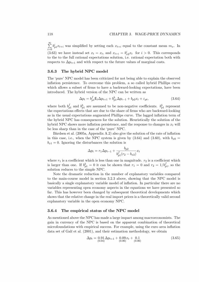
118 CHAPTER 3. WAGE-PRICE DYNAMICS
∞Pi=0
bip1xt+i was simplified by setting each xt+i equal to the constant mean mx. In
(3.63) we have instead set xt = xt, and xt+i = bix2xt for i > 0. This correspondsto the to the full rational expectations solution, i.e. rational expectation both withrespects to ∆pt+1 and with respect to the future values of marginal costs.
3.6.3 The hybrid NPC model
The ‘pure’ NPC model has been criticized for not being able to explain the observedinflation persistence. To overcome this problem, a so called hybrid Phillips curvewhich allows a subset of firms to have a backward-looking expectations, have beenintroduced. The hybrid version of the NPC can be written as
∆pt = bfp1Et∆pt+1 + bbp1∆pt−1 + bp2xt + εpt, (3.64)
where both bfp1 and bbp1 are assumed to be non-negative coefficients. bbp1 representthe expectations effects that are due to the share of firms who are backward-lookingas in the usual expectations augmented Phillips curve. The lagged inflation term ofthe hybrid NPC has consequences for the solution. Heuristically the solution of thehybrid NPC shows more inflation persistence, and the response to changes in xt willbe less sharp than in the case of the ‘pure’ NPC.
Bårdsen et al. (2005a, Appendix A.2) also give the solution of the rate of inflationin this case, i.e., when the NPC system is given by (3.64) and (3.60), with bx0 =bx1 = 0. Ignoring the disturbances the solution is
∆pt = r1∆pt−1 +bp2
bfp1(r2 − bx2)xt
where r1 is a coefficient which is less than one in magnitude. r2 is a coefficient whichis larger than one. If bbp1 = 0 it can be shown that r1 = 0 and r2 = 1/bfp1, so thesolution reduces to the simple NPC.
Note the dramatic reduction in the number of explanatory variables comparedto the main-course model in section 3.2.3 above, showing that the NPC model isbasically a single explanatory variable model of inflation. In particular there are novariables representing open economy aspects in the equations we have presented sofar. This has however been changed by subsequent theoretical developments whichshows that the relative change in the real import prices is a theoretically valid secondexplanatory variable in the open economy NPC.
3.6.4 The empirical status of the NPC model
As mentioned above the NPC has made a large impact among macroeconomists. Thegain in currency of the NPC is based on the apparent combination of theoreticalmicrofoundations with empirical success. For example, using the euro area inflationdata set of Galí et al. (2001), and their estimation methodology, we obtain
∆pt = 0.91(0.04)
∆pt+1 + 0.09(0.06)
xt + 0.1(0.06)
(3.65)
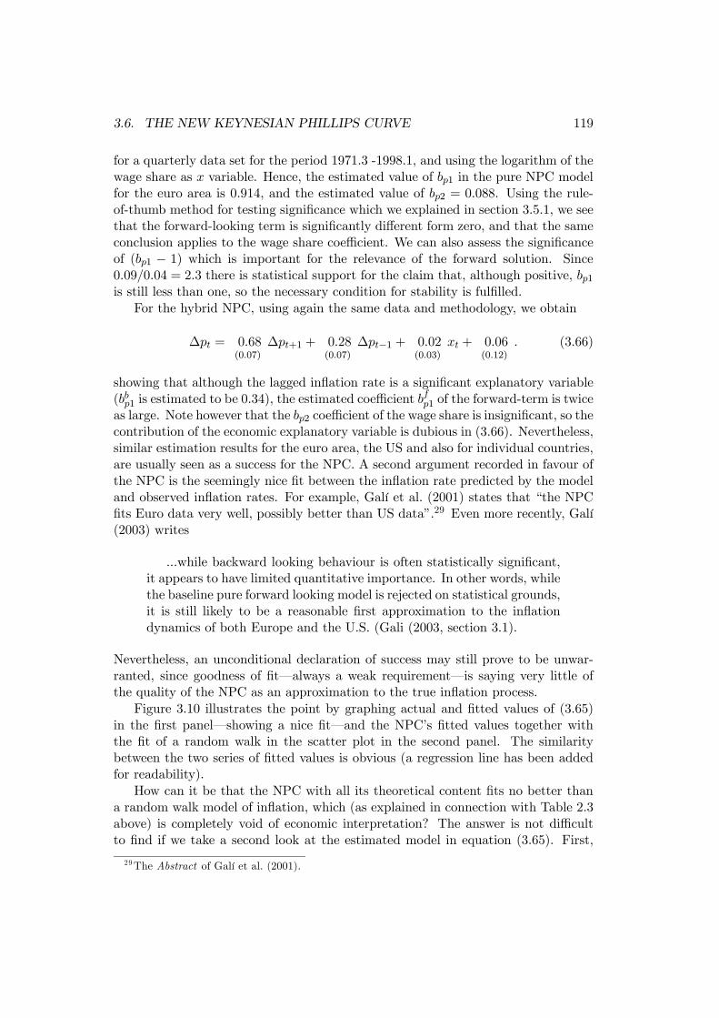
3.6. THE NEW KEYNESIAN PHILLIPS CURVE 119
for a quarterly data set for the period 1971.3 -1998.1, and using the logarithm of thewage share as x variable. Hence, the estimated value of bp1 in the pure NPC modelfor the euro area is 0.914, and the estimated value of bp2 = 0.088. Using the rule-of-thumb method for testing significance which we explained in section 3.5.1, we seethat the forward-looking term is significantly different form zero, and that the sameconclusion applies to the wage share coefficient. We can also assess the significanceof (bp1 − 1) which is important for the relevance of the forward solution. Since0.09/0.04 = 2.3 there is statistical support for the claim that, although positive, bp1is still less than one, so the necessary condition for stability is fulfilled.
For the hybrid NPC, using again the same data and methodology, we obtain
∆pt = 0.68(0.07)
∆pt+1 + 0.28(0.07)
∆pt−1 + 0.02(0.03)
xt + 0.06(0.12)
. (3.66)
showing that although the lagged inflation rate is a significant explanatory variable(bbp1 is estimated to be 0.34), the estimated coefficient b
fp1 of the forward-term is twice
as large. Note however that the bp2 coefficient of the wage share is insignificant, so thecontribution of the economic explanatory variable is dubious in (3.66). Nevertheless,similar estimation results for the euro area, the US and also for individual countries,are usually seen as a success for the NPC. A second argument recorded in favour ofthe NPC is the seemingly nice fit between the inflation rate predicted by the modeland observed inflation rates. For example, Galí et al. (2001) states that “the NPCfits Euro data very well, possibly better than US data”.29 Even more recently, Galí(2003) writes
...while backward looking behaviour is often statistically significant,it appears to have limited quantitative importance. In other words, whilethe baseline pure forward looking model is rejected on statistical grounds,it is still likely to be a reasonable first approximation to the inflationdynamics of both Europe and the U.S. (Gali (2003, section 3.1).
Nevertheless, an unconditional declaration of success may still prove to be unwar-ranted, since goodness of fit–always a weak requirement–is saying very little ofthe quality of the NPC as an approximation to the true inflation process.
Figure 3.10 illustrates the point by graphing actual and fitted values of (3.65)in the first panel–showing a nice fit–and the NPC’s fitted values together withthe fit of a random walk in the scatter plot in the second panel. The similaritybetween the two series of fitted values is obvious (a regression line has been addedfor readability).
How can it be that the NPC with all its theoretical content fits no better thana random walk model of inflation, which (as explained in connection with Table 2.3above) is completely void of economic interpretation? The answer is not difficultto find if we take a second look at the estimated model in equation (3.65). First,
29The Abstract of Galí et al. (2001).
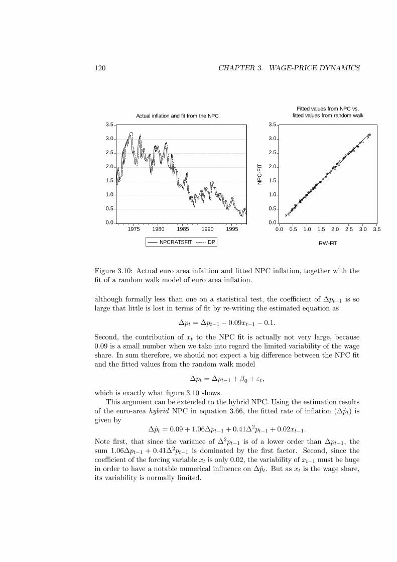
120 CHAPTER 3. WAGE-PRICE DYNAMICS
0.0
0.5
1.0
1.5
2.0
2.5
3.0
3.5
1975 1980 1985 1990 1995
NPCRATSFIT DP
0.0
0.5
1.0
1.5
2.0
2.5
3.0
3.5
0.0 0.5 1.0 1.5 2.0 2.5 3.0 3.5
RW-FIT
NPC
-FIT
Fitted values from NPC vs.fitted values from random walkActual inflation and fit from the NPC
Figure 3.10: Actual euro area infaltion and fitted NPC inflation, together with thefit of a random walk model of euro area inflation.
although formally less than one on a statistical test, the coefficient of ∆pt+1 is solarge that little is lost in terms of fit by re-writing the estimated equation as
∆pt = ∆pt−1 − 0.09xt−1 − 0.1.
Second, the contribution of xt to the NPC fit is actually not very large, because0.09 is a small number when we take into regard the limited variability of the wageshare. In sum therefore, we should not expect a big difference between the NPC fitand the fitted values from the random walk model
∆pt = ∆pt−1 + β0 + εt,
which is exactly what figure 3.10 shows.This argument can be extended to the hybrid NPC. Using the estimation results
of the euro-area hybrid NPC in equation 3.66, the fitted rate of inflation (∆pt) isgiven by
∆pt = 0.09 + 1.06∆pt−1 + 0.41∆2pt−1 + 0.02xt−1.
Note first, that since the variance of ∆2pt−1 is of a lower order than ∆pt−1, thesum 1.06∆pt−1 + 0.41∆2pt−1 is dominated by the first factor. Second, since thecoefficient of the forcing variable xt is only 0.02, the variability of xt−1 must be hugein order to have a notable numerical influence on ∆pt. But as xt is the wage share,its variability is normally limited.
3.6. THE NEW KEYNESIAN PHILLIPS CURVE 121
It is interesting to note that when the NPC is applied to other data sets, i.e., tosuch diverse data as US, UK and Norwegian inflation rates, very similar parameterestimates are obtained, see Bårdsen et al. (2002). Is this a sign of support for theNPC account of inflation? Proponents of the NPC claim so, but another interpreta-tion is that the NPC is almost void of explanatory power, and that it only capturesa common feature among different countries data sets, namely autocorrelation.
Hence, the NPC (as an empirical) model fails to corroborate the theoreticalmessage: that rational expectations transmits the movements of the forcing variablestrongly onto the observed rate of inflation. Recently, it has been shown by ? thatthe typical NPC fails to deliver the expected result that inflation persistence is ‘in-herited’ from the persistence of the forcing variable. Instead, the derived inflationpersistence, using estimated NPCs, turns out to be completely dominated by ‘in-trinsic’ persistence (due to the accumulation of disturbances of the NPC equation).Quite contrary to the consensus view, Fuhrer shows that the NPC fails to explainactual inflation persistence by the persistence that inflation inherits from the forcingvariable. Fuhrer summarizes that the lagged inflation rate is not a ‘second order addon to the underlying optimizing behaviour of price setting firms, it is the model’.
More evaluation of the NPC is provided by e.g., Bårdsen et al. (2004) and Bård-sen et al. (2005a, Ch. 7) which also include testing of parameter stability (oversample periods), sensitivity (with respect to estimation methodology), robustness(e.g., inclusion of a variable such as the output-gap in the model) and encompass-ing (explaining preexisting models.30 Expect for recursive stability, the results aredisheartening for those who believe that the NPC represents a data coherent andtheory driven model of price setting. As for recursive stability, it is more apparentthan real since the inherent fit of the model is so poor that statistical stability testshave low power , and graphs of the sequence of recursive coefficient estimates of theforcing variable show ‘stability around zero’. Even more fundamentally, there is agrowing recognition the NPC model fails on an econometric property called identifi-cation.31 Models with weak or no identification are usually met with suspicion fromall quarters of the economics discipline, but so far the popularity of the NPC hasbeen unscatched by such criticism.
Hence, after evaluation, the economic interpretation of estimated NPC models‘disappears out of the window’ leaving a huge question mark hovering also over theempirical status of New Keynesian DSGE models, of which the DSGE is an integralpart. Despite its initial promises, the NPC modelling approach thus seems to beheading towards a failure. One moment’s thought suffice to make us recognize thatthis may not a surprise. The NPC offers a single variable explanation of inflation,which by all other accounts a complex socio-economic phenomenon, and it is morethan plausible that a satisfactory inflation model will contain more than one ex-planatory variable. As we have seen, this insight was present already in the 1960s,and it has been developed further down the decades in theoretical and empirical
30See also Bårdsen et al. (2002) which includes Norwegian data.31See Mavroeidis (2005).
122 CHAPTER 3. WAGE-PRICE DYNAMICS
models that take account the multi-faceted nature of inflation as a socio-economicphenomena.
That no empirically valid “single cause” explanation of inflation can be providedfor any developed economy is a lesson forgotten by the proponents of the NPCmodel. That said, although the NPC models as they stand, are unsuited for policyrelated economic analysis, this does not preclude that forward-looking expectationsterms could play a role in explaining inflation dynamics within other, statisticallywell specified, models, for example of the equilibrium correction type.
Exercises
1. Is β22 > 0 in (3.16) a necessary and/or sufficient condition for path b to occurin figure 3.2?
2. What might be the economic interpretation of having β21 < 0 , but β22 > 0?
3. Assume that β21 + β22 = 0. Try to sketch the wage dynamics (in other wordsthe dynamic multipliers) following a rise in unemployment in this case!
4. In section 3.3, the expression for the natural rate was found after first estab-lishing the steady state solution for the system. To establish the natural rateof unemployment more directly, rewrite (3.44) as
∆wt = βw1∆mct + βw2(ut −βw0−βw2
) + εw,t, (3.67)
and then the steady state situation: ∆w−gmc = 0, εw,t = 0. Show that (3.67)defines uphil as
0 = βw2[uphil − βw0
−βw2] + (βw1 − 1)gmc.
5. Use the expressions for the wage and price curves in section 3.2.7 to derive thealgebraic expression for uw in figure 3.5.
6. The solution method used for the ‘pure’ NPC on equation (3.56) was based onforward repeated substitution. Section 2.7.1 showed that the ordinary ADL issolved by backward substitution. Why does not backward substitution workfor the NPC?
Hint: The answer has to do with stability. To see why, note that (3.56) canbe re-normalized on ∆pt+1 :
∆pt+1 = (1/bp1)∆pt − (bp2/bp1)xt − (1/bp1) p,t
or∆pt = (1/bp1)∆pt−1 − (bp2/bp1)xt−1 − (1/bp1) p,t−1 (3.68)
i.e., an ADL model (albeit with no contemporaneous effect of and the distur-bance term is lagged). Show that repeated backward substitution using (3.68)gives an unstable solution if 0 < bp1 < 1, confer section 2.7.1 if necessary.
3.6. THE NEW KEYNESIAN PHILLIPS CURVE 123
7. Note that in equation (3.58), giving the solution of the rate of inflation whenthe inflation target is used as a terminal condition, the number of periods aheadj, is a parameter to be determined. With reference to contemporary inflationtargeting, and taking the time period to be annual, it is reasonable to setj = 3. If we assume that the two parameters are known numbers, for examplebp1 = 0.9 and bp2 = 0.1, the inflation rate of period t can be determined usingπ∗ = 0025 and xt = ln(0.5), xt+1 = ln(0.55), and xt+2 = ln(0.65). Work out∆pt, using these numbers in equation (3.58). How is the solution affected ifall three wage shares are 10 percentage points lower?
8. Compare the asymptotically stable solution in equation (3.59) with the stablelong-run solution (2.41) of the ADL model in section 2.7.1. What seems to bethe consequence of forward-looking terms for the stable solution of dynamicrelationships in economics?
9. Consider the NPC estimated on quarterly Norwegian data:32
∆pt = 1.06(0.11)
∆pt+1 + 0.01(0.02)
xt + 0.04(0.02)
∆pbt + dummies
Inflation is measured by the quarterly change in the official Norwegian con-sumer price index. Because of the openness of the economy, the specificationhas been augmented heuristically with import price growth (∆pbt) and dum-mies for seasonal effects as well as the special events in the economy describedin Bårdsen et al. (2002). The estimation period is 1972.4 - 2001.1. xt isthe logarithm of the wage share (total economy minus North-Sea oil and gasproduction).
Compare this equation with the euro area results.
10. Tveter (2005) estimates a NPC for Norway, explaining the domestic part ofthe consumer price index. The sample is 1980.1-2003.3 The xt is defined inthe same way as in the equation in exercise 8. For the pure NPC, Tveterreports
∆pt = 0.95(0.04)
∆pt+1 − 0.001(0.001)
xt,
and for the hybrid model
∆pt = 0.645(0.13)
∆pt+1 + 0.31(0.12)
∆pt−1 − 0.001(0.001)
xt.
Take notes on the similarities between these results and the euro area resultsin the main text.
32 , see Appendix B.

124 CHAPTER 3. WAGE-PRICE DYNAMICS
Appendix A
Variables and relationships inlogs
Logarithmic tranformations of economic variables are used several times in the text,first in section 2.2. Logarithms possess some properties that aid the formulation ofeconomic relationships (model building), and the visual inspection of model and dataproperties in graphs. This appendix reviews some key properties of the logarithmicfunction, and the characteristic of graphs.
Throughout we make us of logarithms to the base of Euler’s number e ≡ 2.171828....,and we use the symbol ln for these natural logarithms. In general, the natural log-arithm of a number or variable x is the power to which e must be raised to yield a,i.e., elna = a.
For reference, we put down the main rules for operating on the natural logarith-mic function (both x and y are positive):
ln(xy) = lnx+ ln y (A.1)
ln(x
y) = lnx− ln y (A.2)
lnxa = a lnx, a is any number or variable (A.3)
From these basic rules, additional ones can be constructed. For example
ln(xayb) = a lnx+ b ln y
which is often called a linear combination of the log transformed variables, withweights a and b. In the main text, a prime example of a linear combination isthe stylized definitional equation for the log of the consumer price index, see e.g.equation (??). In that equation the weights sum to one, corresponding to b = 1−a.Another example of a linear combination is the weighted geometric average:
ln((xy)1/2) = 0.5(ln(x) + ln(y))
125
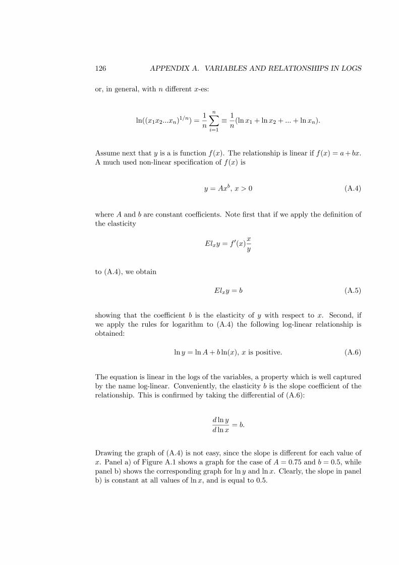
126 APPENDIX A. VARIABLES AND RELATIONSHIPS IN LOGS
or, in general, with n different x-es:
ln((x1x2...xn)1/n) =
1
n
nXi=1
≡ 1
n(lnx1 + lnx2 + ...+ lnxn).
Assume next that y is a is function f(x). The relationship is linear if f(x) = a+ bx.A much used non-linear specification of f(x) is
y = Axb, x > 0 (A.4)
where A and b are constant coefficients. Note first that if we apply the definition ofthe elasticity
Elxy = f 0(x)x
y
to (A.4), we obtain
Elxy = b (A.5)
showing that the coefficient b is the elasticity of y with respect to x. Second, ifwe apply the rules for logarithm to (A.4) the following log-linear relationship isobtained:
ln y = lnA+ b ln(x), x is positive. (A.6)
The equation is linear in the logs of the variables, a property which is well capturedby the name log-linear. Conveniently, the elasticity b is the slope coefficient of therelationship. This is confirmed by taking the differential of (A.6):
d ln y
d lnx= b.
Drawing the graph of (A.4) is not easy, since the slope is different for each value ofx. Panel a) of Figure A.1 shows a graph for the case of A = 0.75 and b = 0.5, whilepanel b) shows the corresponding graph for ln y and lnx. Clearly, the slope in panelb) is constant at all values of lnx, and is equal to 0.5.
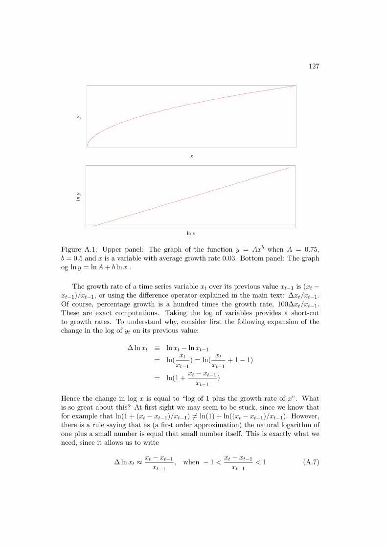
127
y
x
ln y
ln x
Figure A.1: Upper panel: The graph of the function y = Axb when A = 0.75,b = 0.5 and x is a variable with average growth rate 0.03. Bottom panel: The graphog ln y = lnA+ b lnx .
The growth rate of a time series variable xt over its previous value xt−1 is (xt −xt−1)/xt−1, or using the difference operator explained in the main text: ∆xt/xt−1.Of course, percentage growth is a hundred times the growth rate, 100∆xt/xt−1.These are exact computations. Taking the log of variables provides a short-cutto growth rates. To understand why, consider first the following expansion of thechange in the log of yt on its previous value:
∆ lnxt ≡ lnxt − lnxt−1= ln(
xtxt−1
) = ln(xtxt−1
+ 1− 1)
= ln(1 +xt − xt−1xt−1
)
Hence the change in log x is equal to “log of 1 plus the growth rate of x”. Whatis so great about this? At first sight we may seem to be stuck, since we know thatfor example that ln(1 + (xt − xt−1)/xt−1) 6= ln(1) + ln((xt − xt−1)/xt−1). However,there is a rule saying that as (a first order approximation) the natural logarithm ofone plus a small number is equal that small number itself. This is exactly what weneed, since it allows us to write
∆ lnxt ≈xt − xt−1xt−1
, when − 1 < xt − xt−1xt−1
< 1 (A.7)
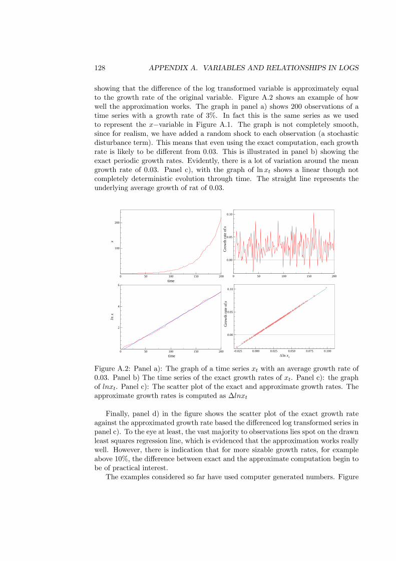
128 APPENDIX A. VARIABLES AND RELATIONSHIPS IN LOGS
showing that the difference of the log transformed variable is approximately equalto the growth rate of the original variable. Figure A.2 shows an example of howwell the approximation works. The graph in panel a) shows 200 observations of atime series with a growth rate of 3%. In fact this is the same series as we usedto represent the x−variable in Figure A.1. The graph is not completely smooth,since for realism, we have added a random shock to each observation (a stochasticdisturbance term). This means that even using the exact computation, each growthrate is likely to be different from 0.03. This is illustrated in panel b) showing theexact periodic growth rates. Evidently, there is a lot of variation around the meangrowth rate of 0.03. Panel c), with the graph of lnxt shows a linear though notcompletely deterministic evolution through time. The straight line represents theunderlying average growth of rat of 0.03.
0 50 100 150 200
100
200
x
time
0 50 100 150 200
2
4
6
time
ln x
0 50 100 150 200
0.00
0.05
0.10
Gro
wth
rate
of x
-0.025 0.000 0.025 0.050 0.075 0.100
0.00
0.05
0.10
Gro
wth
rate
of x
Δln xt
Figure A.2: Panel a): The graph of a time series xt with an average growth rate of0.03. Panel b) The time series of the exact growth rates of xt. Panel c): the graphof lnxt. Panel c): The scatter plot of the exact and approximate growth rates. Theapproximate growth rates is computed as ∆lnxt
Finally, panel d) in the figure shows the scatter plot of the exact growth rateagainst the approximated growth rate based the differenced log transformed series inpanel c). To the eye at least, the vast majority to observations lies spot on the drawnleast squares regression line, which is evidenced that the approximation works reallywell. However, there is indication that for more sizable growth rates, for exampleabove 10%, the difference between exact and the approximate computation begin tobe of practical interest.
The examples considered so far have used computer generated numbers. Figure
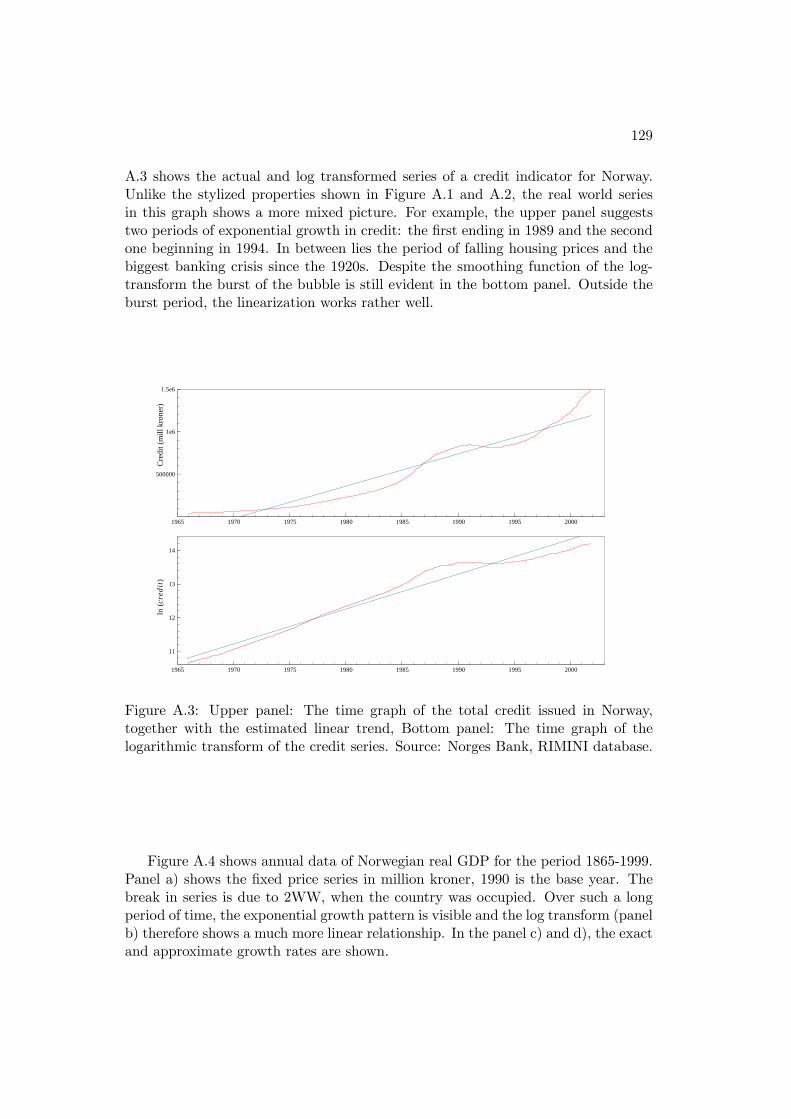
129
A.3 shows the actual and log transformed series of a credit indicator for Norway.Unlike the stylized properties shown in Figure A.1 and A.2, the real world seriesin this graph shows a more mixed picture. For example, the upper panel suggeststwo periods of exponential growth in credit: the first ending in 1989 and the secondone beginning in 1994. In between lies the period of falling housing prices and thebiggest banking crisis since the 1920s. Despite the smoothing function of the log-transform the burst of the bubble is still evident in the bottom panel. Outside theburst period, the linearization works rather well.
1965 1970 1975 1980 1985 1990 1995 2000
500000
1e6
1.5e6
Cre
dit (
mill
kro
ner)
1965 1970 1975 1980 1985 1990 1995 2000
11
12
13
14
ln (c
redi
t)
Figure A.3: Upper panel: The time graph of the total credit issued in Norway,together with the estimated linear trend, Bottom panel: The time graph of thelogarithmic transform of the credit series. Source: Norges Bank, RIMINI database.
Figure A.4 shows annual data of Norwegian real GDP for the period 1865-1999.Panel a) shows the fixed price series in million kroner, 1990 is the base year. Thebreak in series is due to 2WW, when the country was occupied. Over such a longperiod of time, the exponential growth pattern is visible and the log transform (panelb) therefore shows a much more linear relationship. In the panel c) and d), the exactand approximate growth rates are shown.
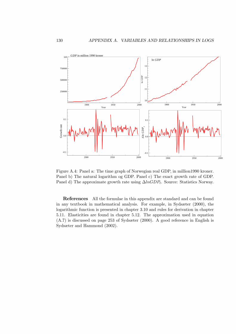
130 APPENDIX A. VARIABLES AND RELATIONSHIPS IN LOGS
1900 1950 2000
250000
500000
750000
1e6 GDP in million 1990 kroner
Year
1900 1950 2000
-0.1
0.0
0.1
Gro
wth
rate
1900 1950 2000
10
11
12
13
ln G
DP
Year
ln GDP
1900 1950 2000
-0.1
0.0
0.1
Δln
GD
Pt
Figure A.4: Panel a: The time graph of Norwegian real GDP, in million1990 kroner.Panel b) The natural logarithm og GDP. Panel c) The exact growth rate of GDP.Panel d) The approximate growth rate using ∆lnGDPt. Source: Statistics Norway.
References All the formulae in this appendix are standard and can be foundin any textbook in mathematical analysis. For example, in Sydsæter (2000), thelogarithmic function is presented in chapter 3.10 and rules for derivation in chapter5.11. Elasticities are found in chapter 5.12. The approximation used in equation(A.7) is discussed on page 253 of Sydsæter (2000). A good reference in English isSydsæter and Hammond (2002).
Appendix B
Linearization of the Solowmodel
In chapter 2.8.3 we derived the well known dynamic equation (2.59) for the capitalintensity variable kt:
kt =1
(1 + n)
©(1− δ)kt−1 + s kγt−1
ªwhich is non-linear because of the last term inside the brackets. With the aid of a firstorder Taylor expansion, see for example Sydsæter and Berck (2006, p. 50), of thatterm we obtain a linearization of the whole expression which gives the approximatedynamics of kt “in the neighbourhood” of the steady state k.
Define the functionf(kt−1) = s kγt−1.
The first order Taylor expansion around the steady-state gives
f(kt−1) ≈ f(k) + f 0(k)(kt−1 − k) (B.1)
= s kγ + γskγ−1(kt−1 − k)
Replacing s kγt−1 in (2.59) by the expression in the second line in (B.1), and collectingterms, gives (2.62) in the main text.
131

132 APPENDIX B. LINEARIZATION OF THE SOLOW MODEL
Bibliography
Aukrust, O. (1977). Inflation in the Open Economy. A Norwegian Model. In Klein,L. B. andW. S. Sâlant (eds.),World Wide Inflation. Theory and recent experience,107—153. Brookings, Washington D.C.
Bårdsen, G., Ø. Eitrheim, E. S. Jansen and R. Nymoen (2005a). The Econometricsof Macroeconomic Modelling . Oxford University Press, Oxford.
Bårdsen, G., Ø. Eitrheim, E. S. Jansen and R. Nymoen (2005b). The Econometricsof Macroeconomic Modelling . Oxford University Press, Oxford. Forthcoming.
Bårdsen, G., E. S. Jansen and R. Nymoen (2002). Model specification and inflationforecast uncertainty. Annales d’Économie et de Statistique, 67/68 , 495—517.
Bårdsen, G., E. S. Jansen and R. Nymoen (2004). Econometric evaluation of theNew Keynesian Phillips curve. Oxford Bulletin of Economics and Statistics, 66 ,671—686. Supplement.
Bårdsen, G. and R. Nymoen (2003). Testing Steady-State Implications for theNAIRU. Review of Economics and Statistics , 85 , 1070–1075.
Birch Sørensen, P. and H. J. Whitta-Jacobsen (2005). Introducing Advanced Macro-economics. McGraw-Hill Education.
Bjerkholt, O. (1998). Interaction between model builders and policy makers in theNorwegian tradition. Economic Modelling , 15 , 317—339.
Blanchard, O. (2005). Macroeconomics. Pearson Prentice Hall, New Jersey, 4th edn.
Blanchard, O. (2009). Macroeconomics. Pearson Education, New Jersey, 5th edn.
Blanchard, O. J. and S. Fisher (1989). Lectures on Macroeconomics. The MITPress, Cambridge, Massachusets.
Blanchard, O. J. and L. Katz (1997). What Do We Know and Do Not Know Aboutthe Natural Rate of Unemployment. Journal of Economic Perspectives , 11 , 51—72.
Blanchard, O. J. and N. Kiyotaki (1987). Monopolistic Competition and the Effectsof Aggregate Demand. American Economic Review , 77 , 647—666.
133
134 BIBLIOGRAPHY
Bruno, M. (1979). Price and Output Adjustment: Micro Foundations and MacroTheory. Journal of Monetary Economics, 5 , 187—212.
Bruno, M. and J. Sachs (1984). Economics of World Wide Stagflation. Blackwell,Oxford.
Burda, M. and C. Wyplosz (2005). Macroeconomics. A European Text.. OxfordUniversity Press, Oxford, 4th edn.
Calvo, G. A. (1983). Staggered prices in a utility maximizing framework. Journalof Monetary Economics , 12 , 383—398.
Driehuis, W. and P. de Wolf (1976). A Sectoral Wage and Price Model for theNetherlands’ Economy. In Frisch, H. (ed.), Inflation in Small Countries, 283–339. Springer-Verlag, New York.
Dunlop, J. T. (1944). Wage Determination under Trade Unions. Reprints of Eco-nomic Classic, 1966. Augustus M. Kelley Publishers, New York.
Edgren, G., K.-O. Faxén and C.-E. Odhner (1969). Wages, Growth and Distributionof Income. Swedish Journal of Economics , 71 , 133—60.
Erlandsen, S. and R. Nymoen (2008). Consumption and population age structure.Journal of Population Economics, 21 (3), 505–520.
Evans, G. and S. Honkapoja (2001). Learning and Expectations in Macroeconomics.Princeton University Press, Princeton, N.J.
Frisch, R. (1929). Statikk Og Dynamikk I Den Økonomiske Teori. Nation-aløkonomisk Tidsskrift , 67 , 321–379.
Frisch, R. (1933). Propagation Problems and Impulse Problems in Dynamic Eco-nomics. In Economic Essays in Honour of Gustav Cassel , 171—205. Allen andUnwin, London.
Frisch, R. (1938). Statistical versus Theoretical Relationships in Economic Macro-dynamics. Memorandum, League of Nations. Reprinted in Autonomy of EconomicRelationships, Memorandum 6. November 1948, Universitetets SocialøkonomiskeInstitutt, Oslo.
Frisch, R. (1947). Notater Til Økonomisk Teori . Universitetets Økonomisk Institutt,Oslo, 4th edn.
Frisch, R. (1992). Statics and Dynamics in Economic Theory. Structural Changeand Economic Dynamics, 3 , 391–401. Originally published in Norwegian in thejournal Nationaløkonomisk Tidsskrift, 67, 1929.
Frisch, R. (1995). Troen På Nøkken. Universitetsforlaget, Oslo. Utvalg og innledningved Andvig, J.C. and O. Bjerkholt and T. Thonstad.
BIBLIOGRAPHY 135
Galí, J. (2003). New perspectives on monetary policy, inflation, and the businesscycle. In Dewatripont, M., L. P. Hansen and S. J. Turnovsky (eds.), Advancesin economics and econometrics. Theory and applicatioms. Eight World Congress,Volume III , chap. 5, 151—197. Cambridge University Press, Cambridge.
Galí, J. and M. Gertler (1999). Inflation Dynamics: A Structural EconometricAnalysis. Journal of Monetary Economics , 44 (2), 233—258.
Galí, J., M. Gertler and J. D. López-Salido (2001). European Inflation Dynamics.European Economic Review , 45 , 1237—1270.
Haavelmo, T. (1943). Statistical Testing of Business-Cycle Theories. The Review ofEconomics and Statistics, XXV (1), 13–18.
Hall, R. E. (1978). Stochastic implications of the life cycle - permanent incomehypothesis: theory and evidence. Journal of Political Economy , 86 , 971—987.
Hendry, D. F. (1995). Dynamic Econometrics. Oxford University Press, Oxford.
Hendry, D. F. (2008). Equilibrium-Correction Models. In Durlauf,S. N. and L. E. Blume (eds.), The New Palgrave Dictionary of Eco-nomics. Palgrave Macmillan, 2nd edn. The New Palgrave Dictio-nary of Economics Online. Palgrave Macmillan. 01 December 2008<http://www.dictionaryofeconomics.com/article?id=pde2008E000284 > doi :10.1057/9780230226203.0496.
Hoel, M. and R. Nymoen (1988). Wage Formation in Norwegian Manufacturing. AnEmpirical Application of a Theoretical Bargaining Model. European Economic Re-view , 32 , 977—997.
Johansen, K. (1995). Norwegian Wage Curves. Oxford Bulletin of Economics andStatistics, 57 , 229–247.
Kaldor, N. (1934). A Classifactory Note on the Determination of Equilibrium. Reviewof Economic Studies, I , 122–136.
Kydland, F. E. and E. C. Prescott (1982). Time to Build and Aggregate Fluctuations.Econometrica, 50 (6 (November)), 1345—70.
Layard, R. and S. Nickell (1986). Unemployment in Britain. Economica, 53 , 121—166.Special issue.
Layard, R., S. Nickell and R. Jackman (1991). Unemployment . Oxford UniversityPress, Oxford.
Layard, R., S. Nickell and R. Jackman (1994). The Unemployment Crises. OxfordUniversity Press, Oxford.
136 BIBLIOGRAPHY
Lindbeck, A. (1993). Unemployment and Macroeconomics. The MIT Press, Cam-bridge.
Lucas, R. E., Jr. (1976). Econometric Policy Evaluation: A Critique. Carnegie-Rochester Conference Series on Public Policy , 1 , 19—46.
Mavroeidis, S. (2005). Identification Issues in Forward-Looking Models Estimated byGMM, with an Application to the Phillips Curve. Journal of Money, Credit andBanking , 37 , 421–448.
Morgan, M. S. (1990). The History of Econometric Ideas. Cambridge University Press,Cambridge.
Nickell, S. J. and M. J. Andrews (1983). Unions, Real-Wages and Employment inBritain 1951-79. Oxford Economic Papers (Supplement), 35 , 183—206.
Nymoen, R. (1989). Modelling Wages in the Small Open Economy: An Error-Correction Model of Norwegian Manufacturing Wages. Oxford Bulletin of Economicsand Statistics, 51 , 239—258.
Obstfeldt, M. and K. Rogoff (1998). Foundations of International Macroeconomics.The MIT Press, Cambridge, Massachusetts.
Roberts, J. M. (1995). New Keynesian economics and the Phillips curve. Journal ofMoney, Credit and Banking, 27 , 975—984.
Rødseth, A. (2000). Open Economy Macroeconomics. Cambridge University Press,Cambridge.
Rødseth, A. and S. Holden (1990). Wage formation in Norway. In Calmfors, L. (ed.),Wage Formation and Macroeconomic Policy in the Nordic Countries, chap. 5, 237—280. Oxford University Press, Oxford.
Romer, D. (1996). Advanced Macroeconomics. McGraw-Hill, New York.
Smets, F. and R. Wouters (2003). An Estimated Dynamic Stochastic General Equi-libirum Model of the Euro Area. Journal of the European Economic Association,1 (5), 1123–1175.
Stølen, N. M. (1990). Is there a Nairu in Norway. Working Paper 56, Central Bureauof Statistics.
Stølen, N. M. (1993). Wage formation and the macroeconometric functioning of theNorwegian labour market . Ph.D. thesis, University of Oslo.
Sydsæter, A. S., K. and P. Berck (2006). Matematisk Formelsamling for Økonomer .Gyldendal Akademisk, Oslo.
Sydsæter, K. (2000). Matematisk Analyse, vol. 1. Gyldendal Akademisk, Oslo, 7thedn.
BIBLIOGRAPHY 137
Sydsæter, K. and P. Hammond (2002). Essential Mathematics for Economics Analysis.Pearson Education, Essex.
Tveter, E. (2005). DSGE Modellens Tilbudsside. Master’s thesis, Universitet i Oslo,Økonomisk institutt.
Wallis, K. F. (1993). On Macroeconomic Policy and Macroeconometric Models. TheEconomic Record , 69 , 113—130.
Wallis, K. F. (1995). Large-Scale Macroeconometric Modeling. In Pesaran, M. H.and M. R. Wickens (eds.), Handbook of Applied Econometrics. Volume I: Macroeco-nomics , chap. 6, 312–355. Blackwell, Oxford.