Southeast Asian Studies. VoL, 24. No. 4. Match 1987

A Medium-term Macroeconometric Modelfor Economic Planning in Indonesia.

Sei KURIBAYASHI**

I Introduction

The five-year development plan which

the Indonesian Government works out

every five years is indicative by nature.

setting policy guidelines for government

development policies. Three development

plans have already been formulated and

carried out since 1969, and implementation

of the Fourth Five-year Development Plan

(Repelita IV) began in April, 1983. In

Repelita IV, macroeconomic mociels were

employed in order to obtain consistency in

macroeconomic aggregates in the economic

framework of the plan. The plan .states:

"Repelita IV has attempted to employ

macroeconomic models as guidance for its

broad quantitative estimates. This has

enabled the plan to take a better account

of the existing interdependencies and

interrelations among variables as well as

among sectors, with a view to obtaining

* I am grateful to Shinichi Ichimura, KazumiKobayashi, Sumimaru Odano, and TakaoOshika for many helpful conversations anduseful comments. I also thank AdrianusMooy and other staff members of A Quanti­tative Study on the Medium/Long.termProspect of the Indonesian Economy for theirwarm hospitality and help during my stay inIndonesia.

** ~*" t!:t. Economic Research Institute, Eco­nomic Planning Agency, 3-1-1 KasumigasekiChiyoda-ku, Tokyo 100, Japan '

350

a better consistency in the planned

macroeconomic aggregates. In this respect

the present plan constitutes a step forward

from the past practice."

The macroeconomic models consist of a

macroeconometric model. an interindustry

model and two submodels. agriculture and

energy, as described in Fig. 1. The

macroeconometric model comprises a core

model, a fiscal submodel. a monetary

submodel and a balance-of-payments

submodel. The core model and each

submodel were constructed and tested

independently at the first stage, then at

the later stage attempts. were made to

integrate them. The monetary submodel,however. was not connected with other

models because of our shortage of com­puter capacity.I) Consequently, the macro-

. econometric model. which consists of thecore model, the fiscal submodel and the

balance-of-payments submodel, was used

for the purpose of conducting simulations

for Repelita IV. The balance of payments

submodel, however, was not completely

1) The monetary submodel was successfullyconnected with the core model, but whenwe tried to integrate the core model withthe monetary submodel as well as the fiscalsubmodel, we encountered difficulties withthe computer capacity. For the monetarysubmodel, see _Ezaki [1982] and Odano[1983a].

S. KURIBAYASHI: A Medium-term Macroeconometric -Model for Economic Planning in Indonesia

2) For detailed explanation of the fiscal sub­model and the balance-of-payments submodel,see Bappenas and Ministry of Finance [1982Jand Odano [1983bJ.

3) The dividing line between low-income andmiddle-income economies is 410 dollars at1982 prices based on the World Bank's classi­fication.

n Economic Developmentin Indonesia

1. Economic Development since

1969

nesian economy in the 1970s and

1980s in terms of macroeconomic

aggregates. Section 3 explains

the structure of the core model.2)

In section 4 multiplier analysis

is briefly presented.

It goes without saying that a

necessary condition for model

builders is to have a good grip

of the characteristics of economic develop­

ment in the past and of problems and

issues of the present and future. First,

therefore, a brief description is given of

the economic development of Indonesia

since 1969 in terms of macroeconomic

aggregates.

Indonesia's per capita gross domestic

product (GDP) was less than 100 dollars

in 1970, about 200 dollars in 1974 and

hit the 300 dollar mark in 1977. Indo­

nesia became one of the lower middle­

income economies in the World Bank's

classification, attaining a per capita GDP

of about 490 dollars in 1980.3) GDP in­

creased at an annual rate of about 20

percent in the 11 years from 1970 through

Fig. 1 Macroeconomic Model for Economic Planningin Indonesia

Macroeconometric MOdel

Fiscal Submodel

Monetary Submodel Core ModelBalance-of-payments

Submodel

Agriculture ISubmodel

Energy ISubmodel.

InterindustryModel

integrated with the core model and the fiscal

submodel, but rather used for checking

purposes, for it did not have feedback

loop to influence the other models, and

exchange rate treated as an exogenous

variable in the macroeconometric model.

The core model was estimated several

times with data for different sample

periods. It was first estimated with the

data for the sample period 1969 to 1980.

Then data for 1981 were added. and it was

re-estimated and revised to give Core

Model-81. Core Model-81 was used for

planning together with other submodels.

It was then re-estimated with the data

from 1969 to 1983 to give Core Model-83.

Other submodels were treated similarly,

and numerical suffixes are added to distin­

guish the different versions and revisions

with different sample periods.

This paper aims mainly to describe the

structure of the core model and to explain

its structural equations. Section 2 describes

the historical development of the Indo-

351

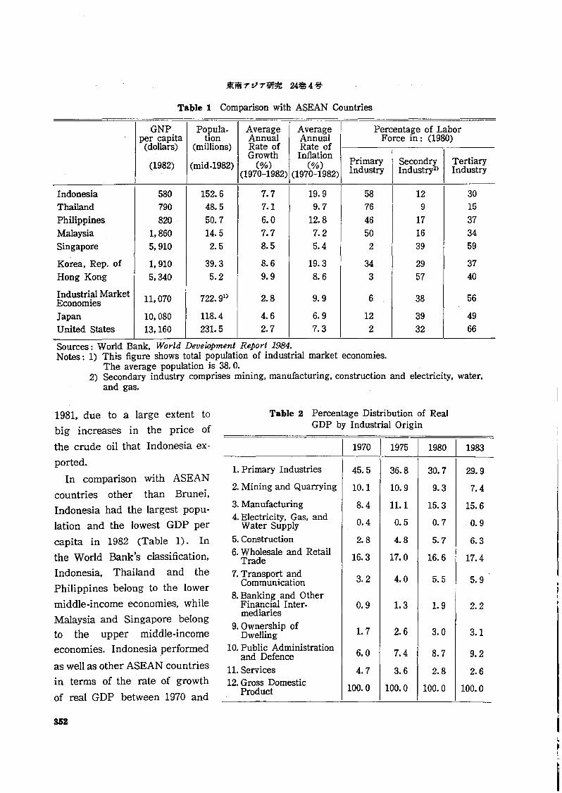
Table 1 Comparison with ASEAN Countries

GNP Popula- Average Average Percentage of Laborper capita tion Annual Annual Force in: (1980)

(dollars) (millions) Rate of Rate ofGrowth Inflation

Primary Secondry Tertiary(1982) (mid-1982) (%) (%)(1970-1982) (1970-1982) Industry Industry2> Industry

Indonesia 580 152.6 7.7 19.9 58 12 30Thailand 790 48.5 7.1 9.7 76 9 15

Philippines 820 50.7 6.0 12.8 46 17 37Malaysia 1,860 14.5 7.7 7.2 50 16 34Singapore 5,910 2.5 8.5 5.4 2 39 59

Korea. Rep. of 1.910 39.3 8.6 19.3 34 29 37Hong Kong 5.340 5.2 9.9 8.6 3 57 40

Industrial Market 11,070 722.9° 2.8 9.9 6 38 56EconomiesJapan 10,080 118.4 4.6 6.9 12 39 49United States 13,160 231. 5 2.7 7.3 2 32 66

Sources: World Bank, World Development Report 1984.Notes: 1) This figure shows total population of industrial market economies.

The average population is 38. o.2) Secondary industry comprises mining, manufacturing, construction and electricity, water,

and gas.

I 1970 I 1975 I 1980 I 1983

Table 2 Percentage Distribution of RealGDP by Industrial Origin

1. Primary Industries 45.5 36.8 30.7 29.9

2. Mining and Quarrying 10.1 10.9 9.3 7.4

3. Manufacturing 8.4 11.1 15.3 15.64. Electricity, Gas, and 0.4 0.5 0.7 0.9Water Supply5. Construction 2.8 4.8 5.7 6.36. Wholesale and Retail 16.3 17.0 16.6 17.4Trade7. Transport and 3.2 4.0 5.5 5.9Communication8. Banking and Other

Financial Inter- 0.9 1.3 1.9 2.2mediaries

9. Ownership of1.7 2.6 3.0 3.1Dwelling

10. Public Administration 6.0 7.4 8.7 9.2and Defence11. Services 4.7 3.6 2.8 2.612. Gross Domestic 100.0 100.0 100.0 100.0Product

1981. due to a large extent to

big increases in the price of

the crude oil that Indonesia ex­

ported.

In comparison with ASEAN

countries other than Brunei,

Indonesia had the largest popu­

1ation and the lowest GDP per

capita in 1982 (Table 1). In

the World Bank's classification,

Indonesia, Thailand and the

Philippines belong to the lower

middle-income economies. while

Malaysia and Singapore belongto the upper middle-incomeeconomies. Indonesia performed

as well as other ASEAN countriesin terms of the .rate of growth

of real GDP between 1970 and

352

S. KURIBAYASHI: A Medium-term Macroeconometric Model for Economic Planning in Indonesia

certain interesting fea­

tures. First, real GOP

follows a conspicuous

growth-rate cycle with

two-year up-swing and

two-year down-swing.Second. as can be

guessed from Table 2,

growth rates of GOP and

primary industry change

almost in parallel except

for 1977. Up to about1976. in particular. the

growth patterns of

mainly agriculture and

mining were reflected in

GOP. Third. the .influ­ences on GOP of maliu­

facturing, construction.

and public administra-

tion and defence have

increased since 1977, though agriculture

and mining were still dominant. Fourth,

the real growth rate of all industries drop­

ped sharply in 1982, and most industries

except agriculture recorded the lowest rate

of growth since 1969. Their rates of

growth were also very low in 1983. In

building a macroeconometric model, it is

extremely important to assess whether this

sharp reduction in the rate of growth of

real GDP is of a temporary nature or more

permanent.

To find out why the growth rate of realGOP dropped suddenly at the beginning

of the 1980s, we also have to examine

GOP by expenditure. Fig. 3, which depicts

growth rates of real GDP by expenditure.

also reveals a few important facts. First.

Transportationand Communication

~.

~. Public Administrationand Defence

Manufacturing

Gross DemesticProduct

a ~ _'.

1970 71 72 73 74 75 76 77 78 79 80 BI 82 83 (year)

Fig.2 Growth Rate of GDP by Industrial Origin

10

24

20

10

24

20

(%)12

10

8

6

4

2

3g 1--'""19~70;;-::7f:-1....,R:b:-~73~74-:-:7:r:5,-:7*6~77:--::!7!:-B -=7:1:9-:B*0~8"'-1-:8!:-2....,83~­

i \ .........Construction'. i ...\,-~"J: \'./\

! 'v( \: ~ \ I: \. .:'"

"'! /\ .: 7',: ".~,j'; Mining \,

O~-r----------'~------..---:,.---:""......,..-+--;..-~--

-10

1982, but had the highest rate of inflation,

19.9 percent. In the industrial structure

of employment, Indonesia has high per­

centage distribution in primary industry

and low one in secondary industry.

Table 2 shows changes in the percentage

distribution of real GOP by industrial

origin. It is clear that the percentage of

primary industry (mainly agriculture)

decreased rapidly while those of manu­

facturing. construction, transportation and

communication, and public administration

and defence increased. Mining, and

wholesale and retail trade maintained

roughly a constant percentage distribution

throughout the decade. Fig. 2, which

depicts changes in annual growth rates of

real GOP by industrial origin. reveals

353

4) Though the export price of crude oil de.creased by five dollars per barrel, the terms oftrade in 1983 improved. This is due to in­creases in export prices of primary goodsbecause of recovery in the world market forthose goods.

ing countries turned out to be an" '1 b " ~ .01 onanza .Lor IndonesIa. Income

was transferred from oil importingcountries to Indonesia and enabledprivate consumption to increase ata much higher rate than GDP. This

is shown more clearly in Fig. 4.which shows annual movement of

the terms of trade of Indonesia.

The terms of trade substantially im­proved in 1974 and in the period1979 to 1981:ll That is to say, Indo­

nesia became able to import three

or four times as many goods andservices as before the increases inthe crude oil price with the sameamount of exports in those years.We can also notice that importsincreased substantially in the same

years. At, the' same time, importsfluctuated almost in parallel with private

<;:onsumption. Second. the rate of increase

in exports decreased after 1976 and realexports even decreased after 1979. It was

due to sharp increases in the exportprice of crude oil that the Indonesian

economy was able to maintain a highgrowth rate in the late 1970s, despite the

deceleration of real exports.The sharp drop in the growth rate of

real GDP in 1982 was caused mainly by a

steep decrease in exports. which was as­cribed to the long-lasting severe world reces­

sion triggered by the second "oil shock."20

/:\../ \

, .\./

"...~'•..•...........

.... j..V

GrossDomesticProduct'

Tirms of Trade ..../

__L : (.J , 10

.... Export Price of Crude Oil.-..­...........19697071 7273 74 7S 76 77 78 79 80 '81 8283(year)

Fig. 0& Terms of Trade and ExportPrice of Crude Oil

10

30

20

(%)

18r--------------16

14

12

10

8

6 .......i\4 .... Private ~.

2 .' Consumption

oha::;;--;fI:.~7~3~-7-=!::-:!:;--=!;;~---:!:~-:!-:~72 ,...~4 7576 77 78 79 80 81 82 83

I .. \! \ Gross DomesticI .. \

:.j..... \

100

(%)300

-10

200

1970 71 72 73 '74 7576 77 78 79 80 81 82 83(Year)

Fig. S Growth Rate of GDP by Expenditure

the rate of increase in private final con­sumption fluctuates almost in parallel with

the growth rate of real GDP, but the formerfar exceeds the latter in 1974 and in the

period 1979 to 1981. This phenomenonmay only be observed in oil-exporting

countries. This is attributable to two bigincreases in the price of exported crude

oil. As Indonesia is an oil-exporting coun­try, the so-called "oil shock" for oil import-

S. KURIBAYASBI: A Medium-term Macroeconometric Model for Economic Planning in Indonesia

In 1983 non-oil exports of Indonesia in­

creased due to the increase in world trade

that accompanied the recovery of the world

economy. especially the economy of the

United States. The growth rate of real

GDP, however, remained low, though it

exceeded the rate in the previous year.

This was caused by the reduction in both

government consumption and investment.

The export price of crude oil was reduced

by five dollars per barrel in March, 1983.

This affected government revenue adversely

and aggravated the balance of payments.

In the face of this economic difficulty, the

Table 3 Annual Growth Rate of Real GDP by Expenditure

1983 11970-1973\1974-197811979-198311969-1981\ 1982

1. Private Consumption 8.5 3.4 7.5 6.1 7.5 10.92. Government Consumption 12.3 8.2 -1.0 15.0 12.3 7.53. Total Investment 14.9 13.0 7.8 22.6 14.2 11.13.1 Private Investment 9.8 24.0 26.2 18.4 8.9 13.13.2 Government Investment 22.6 4.7 -8.5 39.8 23.5 10.1

4. Exports 7.5 -13.9 6.3 16.2 6.3 -3.2(Non-oil/gas Exports) (4.4) (-) (-) (-) (-) (-)

5. Imports 17.0 8.2 12.3 19.1 15.5 17.06. Gross Domestic Product 7.9 2.2 4.2 8.8 7.2 6.1

(5.0*) (6.7*) (6.5*)

Note: *The target growth rate in each five-year plan.

Table 4: Annual Growth Rate of Real GDP by Industrial Origin

1983 11970-197311974-197811979-198311969-19811 1982

1. Primary Industries 3.8 2.1 4.8 4.6 3.0 4.21.1 Agriculture 3.9 3.6 4.8 3.1 3.4 5.51.2 Forestry 3.1 -24.1 3.5 20.8 0.4 -10.71.3 Fishery 3.6 5.5 6.2 1.1 4.3 5.6

2. Mining and Quarrying 7.5 -':'12.1 1.8 16.7 5.0 -1.73. Manufacturing Industries 14.0 1.2 2.2 13.0 13.7 9.74. Electricity, Gas, and Water 13.4 17.4 6.9 11. 7 13.5 14.8Supply5. Construction 16.1 5.2 6.2 23.1 15.2 8.86. Wholesale and Retail Trade 8.0 5.7 3.8 10.3 6.5 8.07. Transport and Communication 13.4 5.9 5.0 13.3 15.1 7.98. Banking and Other Financial 15.4 11. 7 7.0 22.2 14.9 11.0Intermediaries9. Ownership of Dwelling 14.3 5.2 6.1 15.4 15.1 6.9

10. Public Administration and 11.8 3.6 5.5 7.9 13.9 9.1Defence11. Services 2.5 2.3 2.5 2.6 2.4 2.412. Gross Domestic Product 7.9 2.2 4.2 8.8 7.2 6.1

365

Government restrained' its expenditure

severely and devalued foreign exchange.

In this connection, real. government con­

sumption .decreased. by 1. 0 percent and

real government investment by 8. 5 per­

cent (Table 3).

It is crucial to recogniie that Indo­

nesia's external economic environment

became much less favorable in the early1980s than in the 1970s. The five-dollar

reduction in the oil export price was

literally a "reve'rse oil shock" to Indonesia.

This is one of ,key ele~ents of our modelbuilding.

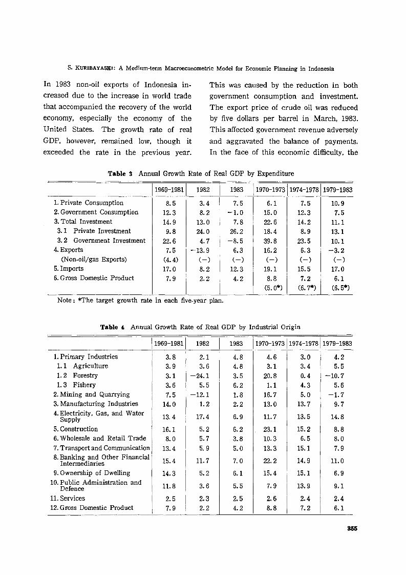
Tables 3 and 4 show respectively the

trends of real GDP by· expenditure and

by industrial origin. Both tables are based

on tlie assumption that growth trends

changed in the. early 1980s. The last threecolumns in both tables show annual average

growth rates for the past three five-year

development plans. Observed growth

rates of real GDP exceeded the targeted

growth rates for Repelita I and RepelitaII, but fell short of those for Repelita III

because of the low growth rates in 1982and 1983. Compared with the previous

two planning periods, the average annual

rates of increase in 1979-1983 decreasedfor m'ost items in both tables. This may

mean ., that as' the scale of the Indonesian

economy increased, the economic· domestic

fronti~rs were reduced and economic deve­

lopment decelerated. The rates of increase

in real value added of forestry and mining

dropped sharply, as did the rate of increasein construction, although this still remained

relatively high.. On the other hand, fishery,

agrictl.1t.u!"~, _~md_ electri<::ity, gas. and water

356

sUPply attained accelerating .. growth rates

through ·the three periods, though the

acceleration was not large.

On the .expenditure 'side, -the rate of

increase in exports dropped sharply, while

private consumption increased at an

accelerating rate. This was attributed tothe "oil bonanza."

Indonesia has given priority to agri­

cultural development to attain self-suffi­ciency in food and to developing and

fostering import substitution industriesmainly in the field of consumption goods.

One ·problem is that the development of

import substitution industries did. notnecessarily lead to export promotion and

Indonesia lagged far behind in developing

export industries. Exports. therefore, 'con­

sist mainly of crude oil and primary pro­ducts. In the 1970s crude oil export

brought in enough foreign currency for

Indonesia to import both consumer goods

and capital goods needed to pursue its

development policies. After 1982, however,Indonesia encountered difficulties in earn­

ing foreign currency and had to employausterity policies. Another important fea­

ture of the Indonesian economy is that

government expenditure, both consumption

and investment, increased at the highest

rate in the 1970s and led the economy.

This is a common feature of almost all

developing countries. Since Indonesia

depends on crude oil export--about 60percent of total export is crude oil and

about '70 percent of government _domesticrevenues is related to oil production -and

export-'-decreases in the export price ofcrude oil and the quantity of crude oil

s. KURIBAYABSI: A Medium-term Macroeconometric Model for Economic Planning in Indonesia

export compelled the Government to

reassess its economic policies and develop­

ment strategies in the early 1980s.

2. Economic Problems in the 1980s

We have seen that Indonesia was con­

fronted with several economic problems

in the early 1980s. These have to be taken

into account in constructing a macroecono­

metric model. Some of them will be touched

upon here.2.1 Reduction of the Excessive Dependence

on Petroleum and LNG

Indonesia depends on crude oil export

in two aspects: to earn the foreign currency

necessary for economic development, and

to finance government expenditure, espe­

cially government development expenditure.

Prospects for the quantity and price of

crude oil export, therefore, are crucial

factors in the future economic develop­

ment of Indonesia. This means that the

Indonesian economy is substantially influ­

enced by the world economic conditions.

Indonesia, therefore. has to reduce its

excessive dependence on crude oil in order

to attain a stable economic growth rate,

by promoting non-oil exports on one handand on the other by changing government

revenue systems so as to increase tax

revenue from sources other than oil com­

panies and by reducing subsidies on re­

fined petroleum products.

2.2 How to Finance the Economic Devel­

opment

Needless to say, developing countries

need foreign as well as domestic capital

in order to achieve adequate economic

development. It is usually difficult, if not

impossible, for developing countries, espe­

cially low-income economies and lower

middle-income economies, to finance their

economic development with only domestic

saving, for their saving rates are very low.

Consequently, they have to earn foreign

currency either by exports or by overseas

financing such as foreign aid, borrowingor direct investment, or by both.

In the 1970s Indonesia earned enough

foreign currency for her rather high

economic development by exporting crude

oil and gas. During the same period the

Indonesian Govenment was able gradually

to reduce the ratio of foreign aid to total

government revenue, while increasing the

share of development expenditure in total

expenditure. Indonesia was, however,

confronted with difficulties in increasing

crude oil export in the face of "the reverse

oil shock" of the early 1980s. High priority,

therefore, needs to be given to the pro­

motion of non-oil exports in place of

crude oil and gas in Repelita IV. On the

other hand. one way to save foreign

currency is to foster and develop import­

substitution industries so as to reduce

imports and improve the balance of pay­

ments. Indonesia has adopted this devel­

opment strategy for consumption goods

industries and obtained good results. One

problem is that the development of import

substitution industries did not necessarily

lead to the development and promotion of

export industries. Another policy measure

for increasing exports and reducing imports

is devaluation of the exchange rate, which

has been done several times in the past.

In the past, however, devaluation of the

367

rupiah contributed to the reduction of

imports but not to the promotion of ex­ports.

Capital goods industries have not yet

been developed in Indonesia, so that in­

creases in public and private investmentserve to increase imports and worsen thebalance of payments, as will be shown

later by multiplier analysis. It is a diffi­

cult and challenging task for policy­

makers to decide what strategies should

be adopted for developing capital goods

industries. Different strategies from those

adopted for consumption goods industriesmight be considered. for their impacts on

others sectors will be more profound andfar-reaching.

2.3 Creation of Employment Opportunity

It is estimated that 1. 5 to 2.°millionmainly young people will enter the labor

market every year in the coming years.

An important task is to create jobs for this

young labor force. According to the input­

output table for 1980, the percentage

distribution of employment among indus­

tries is as follows: primary industry, 54. 1;manufacturing, 9. 6; construction, 3. 0;

wholesale and retail trade, 12. 4; transport

and communication, 2. 8; services and

others, 16.3. It is also well known that

most of the labor force is employed in

small-scale or cottage industries, especiallythose using domestic resources. In the

face of an decelerating economic growth

rate, an economic and social system must

be devised to make effective use of domes­

tic resources and to absorb new entrants

to the labor force.

'2.4 Control of Inflation

SI8

Table 1 showed that the rate of infla­

tion in Indonesia in the period 1970 to

1982 was very high compared with other

countries. Indonesia has been trying toincrease domestic savings by changing

its financial systems. For this purpose,among others, it is crucial to control infla­tion in Repelita IV.

III Medium-term MacroeconometricModel for Economic Planning

1. Basic Framework of Macroeconometric

Models

The major role played by macroecono­

metric models in economic development

planning is that of tracing and estimating

the relationship between economic policy

objectives and policy measures in the

light of past economic development, and

of selecting optimal policy measures for

achieving the policy targets set in order

to solve the problems in the economy.

Our macroeconometric models were,

therefore, designed to assess quantita­

tively the impact of government economicpolicies on a variety of macroeconomic

aggregates, especially target variables. As

mentioned, world economic conditions in­

~uence the Indonesian economy to a large

extent. so that variables representing world

economic conditions also have to be incor­

porated into the macroeconometric models

to, estimate their impact on the Indonesianeconomy. Fig. 5 shows major policy varia­

bles, data variables and target variables.

Main policy variables belong to the

government sector and are closely con­

nected with the fiscal submodel. As far

S. KURIBAYASBI: A Medium-term Macroeconometric Model for Economic Planning in Indonesia

Major Policy Variables

Government Consumption (CG)

Government Investment (IG)

Various Tax Parameters

Price of Refined Oil for Domestic

Consumption (PDROL)

Money Supply (SMB)

Credit Supply to Private Sector (CRPMS)

Exchange Rate (RFEX)

Major Data Variables

World Imports (MWR)

Quantity of Oil Production (QOIL) --\

Export Price of Crude Oil (PXOIL) --;

Quantity of Export of LNG (QXGAS)

Export Price of LNG (PXGAS)

Population (N)

M

o

D

E

L

Target Variables

Growth Rate of Real GDP (GDPR)

Per capita National Income

(NNPIN or GDPIN)

Inflation Rate (PGDP or PCP)

Required Foreign Financing

Required Government Foreign Aid·

Current Deficit in the Balance

of Payments

Labor Balance (LABF and EMP)

Oil Balance

Other Endogenous Variables

Fig.5 Policy and Target Variables in the BAPPENAS Macroeconometric Models

as the government revenue is concerned,

tax parameters are considered as policy

parameters. Although various tax equa-

tions were estimated for the sample pe­

riods, the parameters of tax equations may

be changed so as to estimate the impact

of tax reform on government revenue and

other economic aggregates during the

planning period. Important policy varia­

bles in our models are government con­

sumption, which roughly corresponds to

the central government's routine expendi­

ture, and government investment, which

corresponds to the cental government's

development expenditure less defence ex-

penditure and subsidies on fertilizers.

The Indonesian Government subsidized

petroleum products in the 1970s to keep

their domestic prices much lower than

international market prices of their

equivalents. Facing economic difficulties

at the beginning of the 1980s, the

Government introduced new policies to

reduce the subsidies and to raise the

prices to international levels during Repe­

lita IV. To assess the government policy,

the price of refined oil for domestic con­

sumption was introduced into the core

model as a policy variable. We also

sought to introduce a government-regu­

lated price index, made of prices of com­

modities such as rice and sugar, in order

to assess the impact of government price

policy on the rate of inflation and other

369

variables. But lack of data prevented us

from making an adequate price index,

which should be constructed in the future.

Money supply, which is the nominal

supply of broad money in our model, and

the loans to the private sector, which is

the amount of credit supplied to theprivate sector by the monetary system,

are introduced into our model as govern­

ment monetary policy variables. As men­tioned later, we had difficulty in incor­

porating these variables into the core

model. Exchange rate is one of the most

important policy variables.

The other exogenous variables whichplay an influential role in the macroecono­

metric model are called here "data varia­bles." World imports, quantity of oil pro­

duction, and export price of crude oil

influence crucially the future course of

the Indonesian economy as well as govern­

ment development policies. Population is

treated as a data variable, though it will

be a target variable in the long run with

the promotion of family planning.

The target variables listed in Fig. 5 areamong those required for the economic

indicators in the five-year development

plan. Such endogenous variables as cur­rent balance, rate of inflation and the ratio

of foreign aid to government revenue are

considered as constraints to the govern­

ment policies. The Government pursues

optimal economic development policiessubject to the constraints.

Once endogenous and exogenous varia­

bles are determined, structural equations

have to be specified and estimated with

data for a large enough sample. Broadly,

360

there are two approaches often used in

constructing macroeconomic models fordeveloping countries. One emphasizes thesupply side, based on the assumption that

a shortage of the production capacity ofgoods and services puts a ceiling on the

economic growth of developing countries.

We call this "the supply-side approach."

The other emphasizes the demand side,

based on the assumption that a lack of

demand restricts the economic growth of

developing countries as well as developed

countries. We call this "the demand-side

approach." Ideally, both sides should be

taken into account simultaneously, for in

reality the production and demand sides

interact. Emphasis, however, has to belaid on one side or the other in a small

econometric model with less than one­

hundred equations. A lack of data also

compels us to select one approach. Both

approaches were tried at the beginningof our model building.

First, the supply-side approach was

pursued in the core model. A macro

production function of the Cobb-Douglastype was introduced, and private con­

sumption was to be estimated as a resid­

ual. But various difficulties were encoun­tered in applying the supply-side approach.

One was a lack of data on capital stockand employment. With this approach,

sectoral production functions should be

estimated. But this was impossible be­

cause no data on sectoral capital stock

and employmetnt were available. Even on

the macro basis, no data on gross capital

stock were available. Another difficulty

was that the core model based .on this

S. KURIBAYASHI: A Medium-term Macroeconometric Model for Economic Planning in Indonesia

approach could not predict the economic

slowdowns which occurred in 1982 and

1983. This model also had difficulty pre­

dicting up-swings and down-swings within

the sample period. For these reasons, the

demand-side approach was adopted at the

final stage.

Second, a private consumption function

was introduced, and the production func­

tion was modified slightly and used in a

different functional form for estimating

employment. That is to say, the employ­

ment function was specified based on the

assumption that employment was deter­

mined on the production function, given

the volume of production and capital stock.

The core model based on the demand­

side approach showed much better perfor­

mances in the interpolation and extrapo­

lation tests and could trace the declines

in growth rate in 1982 and 1983.

Third, the supply-side approach was also

applied to the export functions. Exports

were divided into three categories: crude

oil, gas, and non-oil and non-gas (non-oil

exports for short) . In specifying each

export function, export was essentially

estimated as the difference between domes­

tic production and domestic consumption.

Good results, however, were not obtained

for non-oil exports, so that a non-oil

exports function was introduced. As far

as crude oil export was concerned, the

supply-side approach was adopted in the

final version.

After scrutinizing the results of both

approaches, the demand-side approach

was selected for all functions except those

related to crude oil.

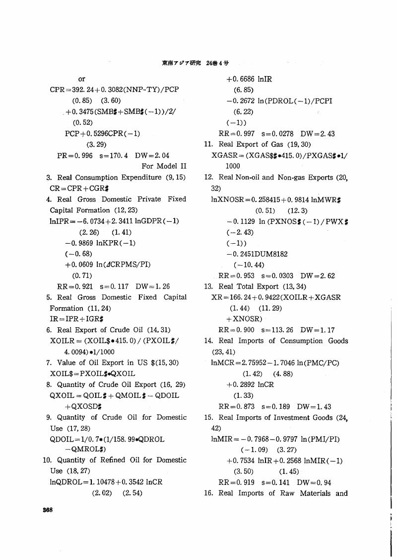
2. Structual Equations of the Core Model

The core model consists of 59 equa­

tions: 21 structural equations and 38 iden­

tities. The fiscal submodel includes 12

tax-and-revenue-sharing equations and one

identity. But only the system of equations

for the core model is shown in the following

"System of Equations." The structural

equations of the core model will be ex­

plained here. Those of the fiscal submodel

are explained in Bappenas and Ministry of

Finance [1982]. Equation numbers in the

following explanations refer to those in the

system of equations.

2. 1 Private Consumption Function (Equa­

tion 2)

The private consumption function in­

cludes real private national disposable in­

come, real money supply and real private

consumption with a one-year time-lag as

explanatory variables. Since Indonesian

national accounts do not include the in­

come and outlay accounts of the house­

hold sector, data on household or personal

disposable income are not available. The

first explanatory variable, (NNP-TY) jPCP,

is a proxy variable for real household

disposable income. The second explanatory

variable, 5MB(-l)jPCP(-l), which is

real money supply at the end of the pre­

vious year, is introduced to represent the

real balance effect, through which money

supply influences other endogenous varia­

bles. Although significant estimates of its

coefficient were not always obtained, this

explanatory variable was included because

the inclusion of money supply in the core

model would have become meaningless

without money supply in the consumption

361

Fig.6 Rates of Increase in Real Private Consumptionand Real Private National Disposable Income

function. Real private consumption with

one-year time-lag, CPR ( -1), is included

based on a distributed lag of the Koycktype.

When the private consumption function

was reestimated with the data extended

up to 1981, the opposite sign was obtained

for the coefficient of real money supply. This

seemed to be caused by an extremely high

rate of increase in real private consump­

tion relative to real private national dis­

posable income in 1981. As Fig. 6 shows,

the rate of increase in real private con­

sumption is extremely high, 16. 7 percent,

despite the relatively low rate of increase,8. 8 percent, in real private national dis­

posable income. This type of movement

was not observed over the sample period

1969 to 1980, although the same phe­

nomenon took place in 1982. A dummy

variable was, therefore, introduced into

Rate of Rate ofIncrease Increase inin CPR (NNP-TY)

/PCP

the private consumption

function in Core Model-81

in order to treat the privateconsumption observation for

1981 as an irregular move­

ment.

30 (%)

This irregularity may be

caused by the compilation

method of private conSump­

tion in the national accounts

of Indonesia. Private coil-

sumption, nominal and real,

is compiled as a residual

between the sum of gross

domestic product and im-

ports and the sum of final

expenditures other than

private consumption and

increases in inventory.According to our estimates, the long­

term prospensity to consume with respect

to private national disposable income was

O. 613 in Core Model-81 and 0.655 in Core

Model-81 and 0.655 in Core Model-83.

2.2 Real Gross Domestic Private Fixed

Capital Formation (Equation 4)

The stock adjustment principle was

employed mainly to provide explanatory

variables for real gross domestic private

fixed capital formation (IPR, real private

investment for short). Real private invest­

ment was regressed on real gross domestic

product with one-year lag (GDPR (-1»,

net capital stock at the end of the pre­

vious year (KPR ( -1) ), and increase in

real credit supply to private sector by

monetary system (CRPMS/PI). Other in­

vestment theories such as the neoclassical

type and Tobin's q could not be tried be-

...,:.....,

20

.....

10-4 0 4

Year

1970

1971

1972

1973

1974

1975

1976

1977

19781979

19801981

1982

1983

(%)

7.6

6.5

12.8

13.018.3

2.7

10.6

7.5

5.2

24.7

14.7

8.8

-3.2

7.9

(%)

3.04.7

5.8

II. 1

14.5

3.6

8.0

4.0

7.514.3

12.7

16.7

'3.4

7.5

382

S. KURIBAYASHI: A Medium-term Macroeconometric Model for Economic Planning in Indonesia

cause of lack of data.

Bank loans to the private sector in­

fluence other endogenous variables through

this equation. although a significant esti­

mate of its coefficient was not obtained.

2. 3 Exports Functions (Equations 6

through 13. 35 through 40)

Exports of goods and services are disag­

gregated into three components: oil. gas,

and non-oil and non-gas exports. Exports

of goods and services in the national

accounts of Indonesia are not divided.

and data on these components had to be

sought from other sources. The sum of

these components. therefore, is not neces­

sarily equal to exports of goods and ser­

vices in the national accounts, but includes

statistical discrepancies. Consequently, the

statistical equations 13 and 39 were esti­

mated in order to complete the model.

2. 3. 1 Crude Oil Export and Quantity

of Refined Oil for Domestic Use

(Equations 6 through 10)

As mentioned, the quantity of crude oil

export (QXOIL) is obtained as the differ­

ence between production and domestic

use, as shown by equation 8.

(1) Crude Oil Export Identity (Equation

8)QXOIL= QOIL# + QMOIL# - QDOIL

+QXOSD#.

where QOIL denotes the quantity of

crude oil production. QMOIL the

quantity of crude oil import. QDOIL

the quantity of crude oil for domestic

consumption and QXOSD statistical

discrepancy, and the symbol # indi­

cates that the variables are exogenous.

.The quantity of refined oil for domestic

consumption QDROL is converted into the

quantity of crude oil by equation 9, which

follows the technical relation for conversion.

(2) Function of the Quantity of Refined

Oil for Domestic Consumption (Equa­

tion 10)

The quantity of refined oil for domestic

consumption (QDROL) is a log-linear func­

tion of real total consumption (CR), real

total investment (IR) and the ratio of price

of refined oil for domestic consumption to

consumer price index (PDROL( -1)/PCPI

( -1) ). The first two explanatory variables

represent income effect and the last one

represents price effect. Though real GDP

was tried as representative of income

effect in place of CR and IR, better results

were not obtained. The difference in

elasticities with respect to consumption

and investment are considered to be rea­

sonable. A reasonable and more-or-Iess

stable estimate of price elasticity was also

obtained as shown in the system of equa­

tions.

It will be desirable in the future version

to break down refined oil products into

main petroleum products such as kerosene.

2.3.2 Real Gas Export (Equation 11)

Gas export (XGASR) is essentially de­

termined exogenously. Almost all of gas

export is LNG. and the quantity is

determined by the long-term production

and export contracts. The export price of

gas (PXGAS) follows that of crude oil,

which is an exogenous variable.

2.3.3 Real Non-oil and Non-gas Exports

Function (Equation 12)

The real non-oil and non-gas exports

(XNOSR) function was specified in accord-

363

ance with the typical theory of demandfunction. The explanatory variables consist

mainly of real world imports (MWR) as the

relevant income variable and the ratio of

price of non-oil exports (PXNOS) to world

export price (PWX) as the relative price

variable. One important channel through

which world economic conditions influence

other endogenous variables is this equation.

A dummy variable was introduced to ex­

plain unusually sharp declines in 1982 and

1983, without which the equation did not

fit well. One reason for the sharp declinewas that Indonesia banned the export of

lumber and changed its policy for shrimp

export. It should be noted that the esti­

mated price elasticity is very low.

2.4 Import Functions (Equations 14

through 18, Identities 44 through 48)

Imports of goods and services are disag­gregated into four components: consump­

tion goods, investment goods. raw materi­

als and intermediate goods, and services

and statistical discrepancy. Like the func­

tion of non-oil exports, all imports wereregressed on a variable representing in­

come effect and a variable representing

price effect.2. 4. 1 Function of Imports of Consump­

tion Goods (Equation 14)

Imports of consumption goods (MCR)

are a function of real total consumption

(CR) and the ratio of import deflator forconsumption goods to consumption deflator

(PMC/PC). A fairly high estimate of price

elasticity of consumption-goods-importsdemand was obtained. This means that

the government policy toward foreign ex­

change can exert a strong influence on

3M

imports of consumption goods, as· will beshown in the multiplier analysis.

2.4.2 Function of Imports of InvestmentGoods (Equation 15)

The long-term elasticity of imports of

investment goods with respect to real in­

vestment in Core Model-81 is O. 945, much

higher than that of imports of consumption

goods. The difference between the elastic­

ities is reflected in the difference between

the multipliers of government consumptionand investment, as will be shown later. In

Core Model-83, the estimated long-termincome elasticity is 1. 014, slightly larger

than 1. 0, although it should be less than

or equal to 1. O. These estimates of coeffi­

cients indicate that almost all investments

have had to be imported because capital

goods industries have not yet been devel­

oped in Indonesia.

2.4.3 Function of Imports of Raw Mate­

rials and Intermediate Goods (Equa­

tion 16)

Real imports of raw materials and inter­

mediate goods were specified as a functionof real GDP (GDPR) and the ratio of im­

port deflator for raw materials and inter­

mediate goods to GDP deflator (PMRM/

PGDP). Fairly stable estimates of the

coefficients were obtained. The fit also

improved as more recent data were addedto the sample.

2. 4. 4 Function of Imports of Services

and Statistical Discrepancy (Equa­

tion 17)

Satisfactory results. were not always ob­

tained in terms of fit, although a stable coeffi­

cient was estimated for each version. This

is due to a defect in the way the data

s. KURIBAYASHI: A Medium-term Macroeconometric Model for Economic Planning in Indonesia

were compiled. The data on imports of ser­

vices and statistical discrepancy (MSDR)

were compiled as the difference between

real imports of goods and services (MR)

in the national accounts and the sum of

MeR, MIR, and MRMR, which were

obtained from other data sources. MSDR,

therefore, includes not only imports of

services but also statistical discrepancy.

The problem is that MSDR accounts for

more than half of MR.

2.5 Depreciation Function (Equation 19)

Depreciation is essentially related to capi­

tal stock. But in practice, firms accelerate

depreciation when they earn better profits,

and vice versa. GDP/capital ratio was

introduced as a profitability variable in

place of profit/capital ratio which was not

available. There are two kinds of real

depreciation introduced in Core Models-81

and 83. One is real total depreciation,

which is needed to derive net national

product from gross national product (see

equations 54 and 55). The other is net

private depreciation, which is used for

deriving real private capital stock (seeequation 20 (2)).

2.6 Employment Function

The employment function is, as men­

tioned, derived from the production function

together with the adjustment principle.

Desired labor demand is assumed to be

determined by the production function,

given capital stock and output. Let EMP*

denote desired labor demand. Then we

have,InEMP* =ao+a1lnGDPR -a21nKR (-1),

where a1>0, a2>0.But firms cannot adjust their employment

to the desired level within one year due to

various costs involved. So they are assumed

to adjust their employment partially. This

is formulated as follows,

(EMP/EMP (-1» =A (EMp·/EMP (-1) ),

where O<.«l.Substituting EMP* into this equation and

taking logarithms of both sides gives the

following labor demand function:

lnEMP = ao.< +a1AlnGDPR - az.<lnKR (-1)

+ (l-A)lnEMP( -1).

The parameter.< represents the speed of

adjustment. If A is large, firms quickly

adjust their employment level to the

desired level. If A= 1, firms adjust their

employment completely within one year.

According to our estimate of A, it takes

firms about two or three years to

adjust their employment to the desired

level.

When we used this employment equa­

tion, we found that the substitution be­

tween capital and labor worked too strongly

in the long-term extrapolation. The capital

stock variable was, therefore, dropped in the

alternative specification of the employmentfunction.

2.7 Labor Force Function (Equation 22)

Labor force (LABF) is simply a func­

tion of population (N). Labor force may

be exogenously determined by demographic

factors. If data on wages were available

they would be introduced into this equa­

tion.

2.8 Price Functions (Equations 25, 26, 27,

and 57)

Two approaches were tried for specify­

ing deflator functions in the core model.

One approach is first to specify GDP defla-

365

tor in accordance with some theory, then

to specify other deflators as a function ofGDP deflator and other variables. Theother is first to estimate individual deflatorfunctions, then to obtain GDP deflator as

the ratio of nominal GDP to real GDP.The latter approach is adopted in most

other macroeconometric models.According to the former, GDP deflator

plays a central and crucial role in pricedetermination. First, the monetary approach

was applied to the specification of the

GDP deflator function in the core model.Good results were not obtained, however,especially for the extrapolation. Conse­quently, the latter approach was adopted in

the final version of the core model. In thiscase, private consumption deflator andinvestment deflator are essential. In each

function the shift parameters of demandand supply functions are basically used as

explanatory variables, for prices are as­sumed to be determined at the intersection

of demand and supply schedules.

GDP deflator is determined as an im­plicit deflator by equation 5l.

2. 8. 1 Private Consumption DeflatorFunction (Equation 25)

Private consumption deflator (PCP) is

a function of real private consumption(CPR), labor productivity (GDPR/EMP),

and price of refined oil for domesticconsumption (PDROL) in Core Model­

81. As mentioned, we sought to intro­duce a government-regulated price indexinto this function. PDROL was introduced

in place of the price index. A dummy

variable was used to eliminate the effect

of the irregularity of private consumption

368

in 1981 and 1982. In the 83 version.unfortunately, a significant estimate was

not obtained for the coefficient of (GDPR/

EMP).

In PCP ICore MOdel-Sllcore Model-83

Canst.-19.4192 -15.6669

(- 3.22) (- 8.85)

In CPR1. 9533 1. 7698

(3.61) (6.92)

In( GDPR ) - 1.0475EMP (- 1.04)

In PDROL 0.3339 0.1323(-1) (1.60) (0.89)

DUMPC- 0.373625 - 0.2294

(- 4. 01) (- 4.01)

R:2 0.986 0.990

2. 8. 2 Consumer Price Index Function(Equation 57)

Consumer price index (PCPI) was simplyregressed on PCP, as both are of thesame kind. PCP covers all goods and

services, whereas the coverage of consumerprice index is limited. The main differ­

ence theoretically is that consumer price

index is of the Laspyres type and PCP isof the Paasche type.

2. 8. 3 Government Consumption DeflatorFunction (Equation 26)

Government consumption consists mainlyof the compensation of government employ­

ees and the goods and services whichthe Government purchases. Government

consumption deflator (PCG) , therefore,

should be a function of the wage rate of

government employees and the price of

the goods and services. But as the wage

S. KURIBAYASHI: A Medium-term Macroeconometric Model for Economic Planning in Indonesia

rate was not available, PCG was regressed

on a kind of domestic demand deflator

(CP+I) / (CPR+IR) = PCP*CPR/ (CPR +

IR) +PI*IR/(CPR+IR).

2. 8. 4 Investment Deflator Function

(Equation 27)

Investment deflator (PI) is a function of

labor productivity, money supply (SMB)

and import deflator of investment goods

(PM!). We tried to introduce real total

investment (IR) in place of 5MB, but a

significant coefficient of productivity could

not be obtained.

Because most investment goods are im­

ported, PMI is assumed to be a dominant

factor for PI, but the assumption was not

fully supported by our results. This may

be ascribed to construction investment.

2.9 Production Function and Capacity

Output (Equations 1 and 58)

The production function of the Cobb­

Douglas type was estimated. The capacity

output equation was derived from the pro­

duction function by shifting the production

function upward by the amount of maxi­

mum residual within the sample period.

(For details, see appendix B in Kuribayashi[1982].)

Capacity output was used in our model

to compare real GDP with capacity output

(GDPRC). GDPR/GDPRC ratio more or

less expresses a kind of capacity utilization.

2. 10 Tax Function (Equations 53 and 56)

Two tax functions were estimated in

the core model: a net indirect tax equa­

tion and a direct income tax equation.

When the core model and the fiscal sub­

model are integrated, these equations are

replaced by the corresponding equations

in the fiscal submodel.

3. System of Equations

Notes: 1. The symbol # denotes exogenous

variables.

2. The first figure in parentheses

after an equation name shows

the equation number in Indo­

nesia's Economic Development

and Bappenas Macroeconometric

Model, 1969-1980 by K. Kobayashi

[1982], and the second figure

is its number in Model Makroe­

konometri Inti Indonesia by

Bappenas [1982].

3. RR denotes the coefficient of

determination adjusted for de­

grees of freedom, s the standard

deviation of disturbances and

DW Durbin-Watson. ratio.

4. The figures in parenthess below

coefficients are t-values of the

coefficients.

5. The sample period is from 1969

through 1983.

1. Real Gross Domestic Product (1, 1)

In (GDPR/EMP) = -0. 885399

(-14.67)

+ O. 6830 In (KR ( -1) /EMP)

(13.94)

RR=O.937 s=0.0461 DW =0.47

For Model I

or

GDPR=CR+IR+XR-.MR

For Model II

2. Real Private Consumption Expenditure

(l0,14)

CPR=GDPR- (CGR+IR+XR-MR)

For Model I

367

or

CPR = 392. 24 + O. 3082(NNP-TY) /PCP

(0.85) (3. 60)

.+0. 3475 (SMBI+SMB#( -1»/2/(0.52)

PCP + O. 5296CPR( -1)

(3.29)

PR=0.996 s=170.4 DW=2.04For Model II

3. Real Consumption Expenditure (9, 15)

CR=CPR+CGR#4. Real Gross Domestic Private Fixed

Capital Formation (12, 23)

InIPR= -6.0734+2. 34111nGDPR( -1)

(2. 26) (1. 41)

- O. 9869 InKPR ( -1)

(-0.68)

+ O. 0609 In (.::1CRPMS/PI)

(0. 71)

RR=0.921 s=0.117 DW= 1. 265. Real Gross Domestic Fixed Capital

Formation (11, 24)

IR = IPR + IGRI

6. Real Export of Crude Oil (14, 31)

XOILR = (XOIL$*415. 0) / (PXOILI/

4.0094)*1/1000

7. Value of Oil Export in US $(15,30)

XOIL$= PXOILI.QXOIL

8. Quantity of Crude Oil Export (16, 29)

QXOIL = QOILI + QMOILI - QDOIL

+ QXOSDI

9. Quantity of Crude Oil for Domestic

Use (17,28)

QDOIL= 1/0. 7* (1/158. 99*QDROL-QMROLI)

10. Quantity of Refined Oil for Domestic

Use (18,27)

InQDROL=1.10478+0.3542InCR

(2. 02) (2. 54)

368

+0.6686 InIR(6.85)

-0.2672 In(PDROL( -1)/PCPI

(6.22)

( -1»

RR=0.997 s=0.0278 DW =2.4311. Real Export of Gas (19,30)

XGASR= (XGAS$I*415. O)/PXGASI*I/1000

12. Real Non-oil and Non-gas Exports (20,

32)

InXNOSR = O. 258415 + O. 9814 InMWRI

(0. 51) (12. 3)

-0.1129 In (PXNOSI (-1) /PWXI(-2.43)

( -1»

- O. 2451DUM8182(-10.44)

RR=0.953 s=0.0303 DW=2.62

13. Real Total Export (13. 34)

XR=166. 24+0. 9422 (XOILR +XGASR(1. 44) (11. 29)

+XNOSR)

RR=0.900 s=113.26 DW=1.17

14. Real Imports of Consumption Goods

(23,41)

InMCR = 2. 75952 -1. 7046 In (PMC/PC)

(1. 42) (4. 88)

+0.2892 InCR

(1. 33)

RR=0.873 s=0.189 DW=1. 43

15. Real Imports of Investment Goods (24,42)

InMIR = - O. 7968 - O. 9797 In (PMI/PI)( -1. 09) (3. 27)

+ O. 7534 InIR + O. 2568 InMIR ( -1)

(3. 50) (1. 45)

RR=0.919 s=0.141 DW=0.94

16. Real Imports of Raw Materials and

s. KURIBAYASHI: A Medium-term Macroeconometric Model for Economic Planning in Indonesia

Intermediate Goods (25, 43)

MRMR = -120. 56 -159. 2 (PMRM/

(-0.75) (-1. 68)

PGDP) + o. 0984 GDPR

(10.43)

RR=0.984 s=48.32 DW=2.01

17. Real Imports of Services and Real

Statistical Discrepancy (26, 44)

InMSDR= -17. 0284+2. 6458 InGDPR

( - 6. 99) (9. 79)

RR=0.871 s=0.3289 DW=1. 34

18. Real Total Import (22, 45)

MR = MCR +MIR +MRMR + MSDR

19. Real Depreciation (8, 3)

(1) DEPR= -745. 65+1216. 97(GDPR/

(-4.44) (5.33)

KR( -1) +0. 0388 KR( -1)

(18.17)

RR=0.987 s=19.49 DM=0.57

(2) DEPPR= -1225.18+ 564. 222 (GDPR/(2. 70) (2. 55)

KPR( -1» +0.1685 KPR( -1)(13.14)

RR=0.982 s=32.34 DW =2.0320. Real Capital Stock (7, 13)

(1) KR=KR( -1) +IR-DEPR

(2) KPR=KPR( -1) +IPR-DEPPR

21. Employment (4, 10)

InEMP=3. 22128+0.1702 InGDPR(2. 33) (2. 19)

+ O. 5587 InEMP (-1)

(2.89)

RR=0.994 s=0.00938 DW=0.84

For Model Ior

InEMP=2. 21448+0.2273 InGDPR

(1. 80) (3. 28)

- O. 0862 InKR ( -1)

(2.39)

+0.6810 InEMP( -1)(4.00)

RR=0.996 s=0.00786 DW=1.52For Model II

22. Labor Force (5, 11)

LABF= -26331. 6+0. 5635N#

( -18. 11) (52. 38)

RR=0.995 s=550.85 DW=0.4023. Unemployment (6,12)

UNEM = LABF - EMP

24. Real Gross National Product (2, 2)

GNPR=GDPR+NFIAR#

25. Private Consumption Deflator (32, 16)

InPCP = -15. 6669 + 1. 7698 InCPR(-8.85) (6.92)

+0.1323 InPDROL( -1) +0.2294

(0.89) (-4.01)

DUM 7080

RR=0.990 s=0.0641 DW =1. 2826. Government Consumption Deflator (29,

17)

PCG= -0. 0642 + 1. 0396 «CP+I) j (CPR( -1. 04) (70. 03)

+IR»RR=0.997 s=0.0684 DW=2.26

27. Investment Deflator (30,25)

InPI= -4. 4014-0. 4412 In(GDPRjEMP)(-2.27) (-0.69)

+0.5201 InSMB#+O.1351 InPMI(4.41) (1. 45)

RR=0.994 s=0.0495 DW=l. 57

28. Nominal Private Consumption Expen­diture (44 or 31, 20)

CP=PCP.CPR

29. Nominal Government Consumption Ex­penditure (45,21)

CG=PCG.CGR

30. Nominal Total Consumption Expendi­

ture (43, 22)

389

C=CP+CG31. Total Consumption Deflator ( , 18)

PC=C/CR32. Nominal Gross Domestic Private Fixed

Capital Formation

IP=PI*IPR33. Nominal Government Investment

IG=PI*lGR34. Nominal Gross Domestic Fixed Capital

Formation (46, 26)

I=PI*IR (=IP+IG)35. Nominal Oil Export (48,36)

XOIL = XOIL$*RFEXI*I/100036. Nominal Gas Export (49.39)

XGAS = XGASI*RFEXI*I/100037. Nominal Non..oil and Non-gas Exports

(50.38)

XNOS = XNOS$*RFEXI*1/100038. Value of Non-oil and Non-gas Exports

in US $ (21, 37)

XNOS$= XNOSR*PXNOSI*1000/415. 039. Nominal Total Export (47,40)

X= -74. 40+1.0489 (XOIL+XGAS

( -1. 01) (115. 22)

+XNOS)RR=0.999 5==196.9 DW=1.42

40. Export Deflator (34, 35)

PX=X/XR41. Import Deflator for Consumption Goods

(36,46)

PMC = PMC$I*RFEX#/415. 042. Import Deflator for Investment Goods

(37.47)

PMI = PMI$#*RFEX#/415. O·

43. Import Deflator for Raw Materials and

Intermediate Goods (38, 48)

PMRM = PMRM$#*RFEXI/415. 044. Nominal Imports of Consumption Goods

(52.50)

870

MC=PMC*MCR45. Nominal Imports of Investment Goods

(53.51)

MI=PMI*MIR

46. Nominal Imports of Raw Materials and

Intermediate Goods (54,52)

MRM= PMRM*MRMR

47. Nominal Imports of Services and Sta­

tistical Discrepancy (55, 53)

MSD = PMSDI*MSDR48. Nominal Total Import (51, 54)

M=MC+MI+MRM+MSD49. Import Deflator (35, 49)

PM=M/MR·

50. Nominal Gross Domestic Product (39,

6)

GDP=C+I+X-M

51. Deflator for Gross Domestic Product(28,5).

PGDP= GDP/GDPR

52. Nominal Gross National Product (40,

7)

GNP=GDP+PM*NFIAR

53. Nominal Net Indirect TaxTI=141. 46+0. 03196 GDP

(3. 89) (28. 79)

RR=0.983 s=94.85 DW=l. 2054. Nominal Depreciation (42, 8)

DEP = PGDP*DEPR55. Nominal Net National Product (41, 9)

NNP=GNP-DEP-TI

56. Direct Income Tax

TY = -47. 66+0. 02871 NNP( -1. 88) (32. 03)

RR=0.987 s=66.11 DW=1. 27

57. Consumer Price Index (33,19)

InPCPI = 3. 85035 + 1. 02984 InPCP(208.66) (45.22)

RR=0.993 s=0.0573 DW=0.93

S. KURIBAYASHI: A Medium-tenn Macroeconometric Model for Economic Planning in Indonesia

C

CP

CG

CPR

duct

= Real Gross DomestLc Product

= Real Capacity Output

= Nominal Gross National Pro­duct

= Real Gross National Product

= Nominal Gross Domestic FixedCapital Formation

= Nominal Gross Government

Fixed Capital Formation= Real Gross Government Fixed

Capital Formation

= Nominal Gross Domestic Pri­

vate Fixed Capital Formation

= Real Gross Domestic Private

Fixed Capital Formation

= Real Gross Domestic Fixed

Capital Formation

= Real Private Capital Stock

= Real Total Capital Stock

= Total Labor Force

=Nominal Total Import

= Nominal Imports of Consump­

tion Goods

= Real Imports of Consumption

Goods

=Nominal Imports of Investment

Goods

= Real Imports of Investment

Goods

= Real Total Import

=Nominal Imports of Raw Mate­

rials and Intermediate Goods

= Real Imports of Raw Materials

and Intermediate Goods

= Nominal Statistical Discrepancy

for Import Sector

= Real Statistical Discrepancy for

Import Sector

MSDR

MSD

MRMR

IR

MIR

MI

MCR

MR

MRM

IPR

KPR

KR

LABF

M

MC

IP

IGR#

IG

GDPR

GDPRC

GNP

GNPR

I

EMP

GDP

CGR#

4. Notation of the Variables

Notes: 1. The symbol # denotes exogenous

variables.

2. Real = 1973 constant price.

Nominal = current price.

= Nominal Consumption Expen­

diture

= Nominal Government Consump­

tion Expenditure

= Real Government Consumption

Expenditure= Nominal Private Consumption

Expenditure

= Real Private Consumption Ex­penditure

CR = Real Consumption ExpenditureCRPMS# = Amount of Credit Supply to

Private Sector by Monetary

System

DEP = Nominal DepreciationDEPPR = Real Private Depreciation

DEPR = Real Depreciation

DUM7080=Dummy Variable for Private

Consumption Deflator (1 for

1970-1980, 0 for 1980-1983)

DUM8182=Dummy Variable for Non-oil

and Non-gas Exports (1 for

1981-1982, 0 otherwise)

=Total Employment

= Nominal Gross Domestic Pro-

58. Capacity Output

In(GDPRCjEMP) = -0. 86840

+0.6830 In(KR( -l)jEMP)

59. Real Net Factor Income from Abroad

NFIAR= -68.11-0.1884(XOIL+XGAS)

(-2.32) (-14.29)

jPM

RR=0.936 s=65.0 DW=1. 46

371

PMI

PM

PMC

PGDP

PI

MWR#

N#NFlA

QOIL#

QXGAS

QXOIL

PXOIL# =Export Price of Crude Oil in

US $ per barrel

PWX# = World Export PriceQDOIL = Quantity of Crude Oil for Do­

mestic Consumption in millionbarrels

QDROL =Quantity of Refined Oil for

Domestic Consumption in mil­

lion liters

QMOIL# =Quantity of Crude Oil Import

in million barrelsQMROL# =Quantity of Refined Oil Import

in million barrels= Quantity of Oil Production

. =Quantity of Export of LNG

= Quantity of Crude Oil Export

in million barrels

QXOSD# = Statistical Discrepancy for the

Quantity of Oil Export

= Rate of Foreign Exchange

= Nominal Supply of Broad Money

=Nominal Net Indirect Tax

=Time Trend=Real Net Indirect Tax

= Direct Income Tax

= Unemployment

= Nominal Total Export

= Nominal Value of Gas Export

in billion Rp

XGAS$# =Nominal Value of Gas Export

in million US $XGASR =Real Gas Export in billion Rp

XNOS =Nominal Value of Non-oil andNon-gas Export in billion Rp

XNOS$ =Nominal Value of Non-oil and

Non-gas Exports in million US $

XNOSR = Real Non-oil and Non-gas

Exports in billion Rp

= Nominal Value of Crude OilXOIL

RFEX#

5MB#TI

TIME#TIR

TYUNEM

X

XGAS

NNP

NNPR

PC

PCG

=Real World Imports

= Population

= Nominal Net Factor Incomefrom Abroad

NFIAR = Real Net Factor Income from

Abroad

=Nominal Net National Product

=Real Net National Product

= Consumption Deflator

= Government Consumption

DeflatorPCP = Private Consumption Deflator

PCPI = Consumer Price Index

PDROL# =Price of Refined Oil for Dome-

stic Consumption

= GOP Deflator= Fixed Capital Formation De­

flator

= Import Deflator

= Import Deflator for Consump­

tion GoodsPMC$# = Dollar Price Index for Con­

sumption Goods Imports= Import Deflator for Investment

Goods

PMI$# = Dollar Price Index for Invest-

ment Goods Imports

PMRM = Import Deflator for Raw Mate­

rials and Intermediate Goods

PMRM$# = Dollar Price Index for Raw

Materials and IntermediateGoods Imports

PMSD# = Import Deflator for Services

and Statistical Discrepancy

PX = Export Deflator

PXGAS# = Price Index of Gas Export in

US $PXNOS# =Price Index of Non-oil and

Non-gas Exports in US $

372

S. KURIBAYASHI: A Medium-term Macroeconometric Model for Economic Planning in Indonesia

Export in billion Rp

XOIL$ = Nominal Value of Crude Oil

Export in million US $

XOILR = Real Crude Oil Export inbillion Rp

XR = Real Total Export

IV Multiplier Analysis

One of the primary advantages of mak­

ing use of econometric models for econo­

mic planning is to be able to evaluate

policy effects quantitatively. The short­

and medium-term impacts of policy varia­

bles on target variables are analysed with

Core Model-81 in this section.

To measure the impacts of changes in

an exogenous variable on endogenous

variables. all endogenous variables are first

solved over the pre-assigned period with

given values of all exogenous variables.

This set of estimates of all endogenous

variables is usually called a "control solu­

tion" or "standard solution." Second, the

values of specific exogenous variables are

changed by a fixed amount and the model

is solved for endogenous variables. We

call this set of values of all endogenous

variables a "disturbed solution." Then.

the impacts can be assessed by comparing

the disturbed solution with the control

solution, the differences between them

usually being taken.

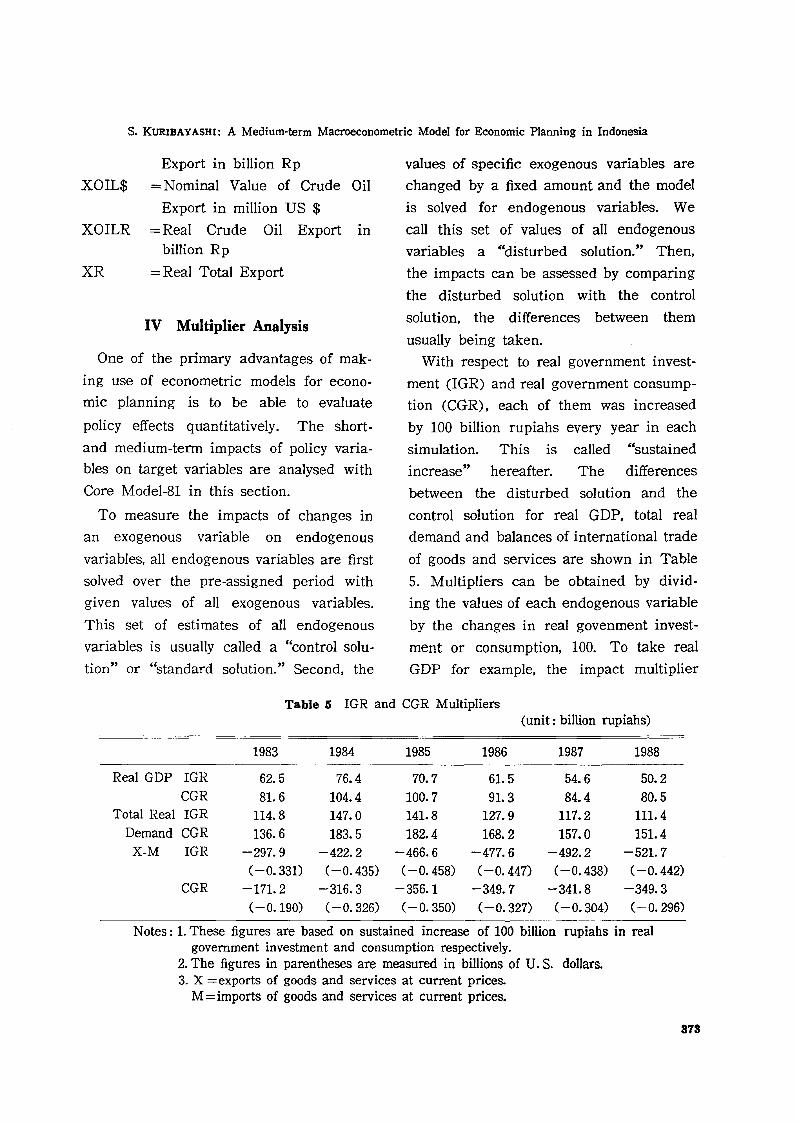
With respect to real government invest­

ment (IGR) and real government consump­

tion (CGR) , each of them was increased

by 100 billion rupiahs every year in each

simulation. This is called "sustained

increase" hereafter. The differences

between the disturbed solution and the

control solution for real GDP. total real

demand and balances of international trade

of goods and services are shown in Table

5. Multipliers can be obtained by divid­

ing the values of each endogenous variable

by the changes in real govenment invest­

ment or consumption, 100. To take real

GDP for example, the impact multiplier

Table 5 IGR and CGR Multipliers(unit: billion rupiahs)

1983 1984 1985 1986 1987 1988

Real GDP IGR 62.5 76.4 70.7 61. 5 54.6 50.2CGR 81. 6 104.4 100.7 91. 3 84.4 80.5

Total Real IGR 114.8 147.0 141.8 127.9 117.2 111.4Demand CGR 136.6 183.5 182.4 168.2 157.0 151.4X-M IGR -297.9 -422.2 -466.6 -477.6 -492.2 -521. 7

(-0.331) (-0.435) (-0.458) (-0.447) (-0.438) (-0.442)CGR -171. 2 -316.3 -356.1 -349.7 -341.8 -349.3

( -0.190) (-0.326) (-0.350) (-0.327) (-0.304) (-0.296)

Notes: 1. These figures are based on sustained increase of 100 billion rupiahs in realgovernment investment and consumption respectively.

2. The figures in parentheses are measured in billions of U. S. dollars.3. X =exports of goods and services at current prices.

M= imports of goods and services at current prices.

373

Jl(M7'~"1'iJm 24~4-8"

Table 8 QOIL, PXOIL, and RFEX Multipliers'

1984 1985 1986 1987 1988 1989

Growth Rate of QOIL , 0.08 0.11 0.10 0.08 0.07 0.05Real GDP PXOIL 0.04 0.05 0.05 0.03 0.02 0.01

(%) RFEX 0.44 0.56 0.50 0.39 0.30Total Tax QOIL 80.0 275.5 530.0 859.4 1276.9 1783.1

(billion PXOIL 84.4 270.3 494.0 766.8 1074.3 1420.5rupiahs) RFEX 595.8 2440.6 4792.2 7620.6 10933.0

X·M QOIL 0.120 0.256 0.413 0.597 0.813 1. 043(billions of PXOIL 0.133 0.265 0.415 0.573 0.726 0.885U.S. dollars) RFEX 0.744 1.593 2.668 4.064 5.863

Notes: 1. Sustained one-percent increase for QOIL and PXOIL.2. Sustained five-percent increase for RFEX.

is 0.625, and the medium-term multiplier

reaches its highest value, O. 764, in the

second year and declines in subsequent

years. In developed countries such as the

United States and Japan, the impact

multiplier is usually around 1. 3 and the

medium-term multiplier peaks at around

2. O. These low multipliers for real govern­

ment investment in the Indonesian economyare ascribed to high leakage through direct

alld indirect imports, as mentioned above

concerning import functions. According

to an econometric model for the Republic

of Korea constructed by the Economic

Research Institute~: Economic PlanningAgency, Japan, government investment

multipliers are also less than 1. O. This

may be a common feature of developing

countries. In comparison with IGR multi­pliers, CGR multipliers, which are slightly

larger than 1. 0 at the peak, ,are larger.

Instead of a sustained, fixed amount of

increase in an exogenous variable, the im­

pacts of a sustained percentage increase

were estimated for the quantity of crude

oil production (QOIL), export price of

374

crude oil (PXOIL) and foreign exchangerate (RFEX), and are shown in Table 6.

Comparison between QOIL and PXOIL

shows that the sustained one-percent in­

crease in crude oil production has a larger

effect than the same increase in the ex­

port price of crude oil. Simply dividing

the results for RFEX by five tells us that

a sustained one-percent devaluation of

foreign exchange has the same effects on

the growth rate of real GDP as the same

increase in crude oil production, but much

larger effect on tax revenue and trade

balance.

V Concluding Remarks

As mentioned in Repelita IV, macroecono­

mic models were employed in. order to

obtain a better consistency in the planned

macroeconomic aggregates. Numerous

policy simulations. were conducted with

the macroeconometric model before a final

conclusion was reached. In our experience

with Indonesian development planning,

macroeconometric models can playa central

s. KURIBAYASHI: A Medium-term Macroeconometric Model for Economic Planning in Indonesia

role and give fresh and deep insights into

the problems and issues in the future and

policy measuses for dealing with them.

One advantage of employing macro­

econometric models for economic plan­

ning is that the actual course of the

economy can easily be compared quanti­

tatively with the planned one, and the

planned policy measures can be revised

if necessary, while implementing the plan

year by year. This means that a rolling

plan can be introduced.

For that purpose, the macroeconometric

models have to be re-estimated with ex­

tended data and revised every year if

necessary. The core model and the fiscal

submodel have so far been re-estimated

three times. Fairly stable parameters were

estimated for structural equations, although

a one-year extension of the data has a

significant influence because of the small­

ness of the sample size.

Needless to say, there exist several

shortcomings in the core model, which

are mainly attributable to lack of data.

These shortcomings have to be remedied

and the core model revised in the follow­

ing directions.

(1) Price equations have to be revised,

introducing wage rate and govern­

ment-regulated price index into them.

In particular, the investment deflator

function needs to be re-specified

without money supply in the explana­

tory variables.

(2) It is desirable that the quantity of

refined oil for domestic consumption

should be disaggregated into com­

ponents such as kerosene. This will

be closely related to the energy sub­

model which has not yet been com­

pleted.

(3) If available, data on imports of invest­

ment goods which are directly related

to government investment should be

compiled and used in the core model.

(4) It is desirable that non-oil exports

should be disaggregated at least into

primary commodities, manufactured

goods, and services.

(5) Reliable data on labor force, employ­

ment, and population have to be com­

piled, because they belong to the most

important economic indicators in the

Indonesian economy.

(6) Indonesian national accounting data

do not include national disposable in­

come and its appropriation accounts

and income and outlay accounts by

institutional sectors. Although this

shortcoming is common in developing

countries, high priority should be

given to their compilation. If they are

provided, our models will be markedly

improved.

(7) Our macro models will be improved

and refined by comparing them with

macro models of other developing

countries. In other words, some study

and research will be needed on con­

structing the same kind of macro

models for other developing countries.

References

Ezaki, MitSllO. 1982. A Monetary Submodel ofthe Bappenas Model. National DevelopmentPlanning Agency (Bappenas) , IndonesianGovernment. (Mimeographed)

Indonesia, Bappenas. 1982. Model Makroekonometri

375

Inti Indonesia. Bappenas, IndonesianGovernment. (Mimeographed)

Indonesia. Bappenas; and Ministry of Finance.1982. An Econometric Analysis oj IndonesianFiscal Sector--A Tentative Report--. Bap­penas, Indonesian Government. (Mimeo­graphed)

Kobayashi, Kazumi. 1982. Indonesia's EconomicDevelopment and Bappenas MacroeconometricModel, 1969-1980. Bappenas, IndonesianGovernment. (Mimeographed)

Kuribaya,shi. Sei. 1982. Revised Core Macro Econo­metric Model. Bappenas. Indonesian Govern­ment. (Mimeographed)

---. 1983a. Revised Core Macro EconometricModel Re-estimated. Bappenas, IndonesianGovernment. (Mimeographed)

3'18

---. 1983b. Multiplier Analysis by the MacroEconometric Model. Bappenas, IndonesianGovernment. (Mimeographed)

Odano, Sumimaru. 1983a. Re-estimation of theEzaki Model oj the Indonesian Monetary Sector.Bappenas. Indonesian Government. (Mimeo­graphed)

---,. 1983b. Indonesian Balance oj Payments.Bappenas. Indonesian Government. (Mimeo­graphed)

Oshika. Takao. 1984. Revised Core Macro Econo­metric Model Re-estimated. Bappenas, Indo­nesian Government. (Mimeographed)

The Technical Team. 1982. Bappenas Core Macro­econometrtC Model. Bappenas, IndonesianGovernment. (Mimeographed)