the robustness of empirical models for unemployment. a ...folk.uio.no/rnymoen/victoriamain.pdf ·...
TRANSCRIPT

The robustness of empirical models for unemployment.
A review of Nickell, Nunziata, and Ochel (2005).
Victoria Sparrman Department of Economics, University of Oslo.
Very Preliminary, please do not cite
November 17, 2008
Abstract
A number of recent papers have tried to explain the evolution of unemployment
in the OECD area, based on an equilibrium unemployment framework. One of
the most influential is Nickell et al. (2005). They find that institutions explains
most of the variation in unemployment for 20 OECD countries from 1960 to 1995.
However, the importance of Nickell et al. (2005) has also spurred a lively debate,
and several papers have criticized their findings. This paper re-asses the findings
of Nickell et al. (2005), benefitting from nine additional years of data. A dynamic
simulation of unemployment by using the model in Nickell et al. (2005), I find a
clear tendency that the model underpredicts the change in unemployment. The
dynamic simulation of unemployment illustrates that actual unemployment rate is
higher than simulated by the empirical model for 13 countries. The unemployment
rate is substantially lower than simulated for 4 countries. Furthermore, I evaluate
the empirical model by implementing some of the critiques into the original model
of Nickell et al. (2005).
1

1 Introduction
The theory for equilibrium unemployment is determined by the behavior of the wage and
price setters in an imperfect market. The price setters are firms sets prices in a non
competitive environment dependent on the development of nominal wages. This is the
price curve, i.e. a relationship between real wage and unemployment. The wage setters
decides on nominal wages given the price level. This is another relationship between
wage and employment. The intersection between the two curves determines the level of
equilibrium unemployment.
A number of recent papers have tried to explain the evolution of unemployment in the
OECD area, based on an equilibrium unemployment framework. One of the most influen-
tial is Nickell et al. (2005). They find that the development in labor market institutions
can account for 55 percent of the increase in European unemployment for the period 1960
to 1995. The effect of institutions to unemployment is equal for all countries in the panel.
The panel consists of 20 OECD-countries.
There are several reasons to re-asses the paper by Nickell et al. (2005). First, the
results are strong, explaining the bulk of variation in unemployment by variation in insti-
tutions.. It is impressive to achieve homogenous results of institutions for all the countries
in the panel. Secondly, the strand of research focussing on the link between labour market
institutions and unemployment has been very influential. Nickell et al. (2005) is a major,
recent contribution to this strand, spurring a lively debate and receiving 267 references in
Google Scholar. The recommendations of international organizations like OECD for how
countries should organize the economies efficiently are heavily influenced by this strand.
Thus, the results of strand of research have been interpreted as a recommendation to
countries for how they should change their institutions in order to avoid or reduce unem-
ployment. The institutions that affects unemployment negatively are benefit replacement
ratio, employment protection, union density and taxes should be reduced to achieve lower
unemployment rate.
This paper evaluates the results in Nickell et al. (2005) over the extended sample 1995
to 2004. A dynamic simulation of the model for unemployment with the original estimated
coefficients illustrates how well the model simulate actual unemployment out of sample.
The actual unemployment rate is higher than simulated by the empirical model for 13
2

countries. The unemployment rate is substantially lower than simulated for 5 countries.
The difference between simulation and actual unemployment rate for the period 1995 to
2004 motivates a closer look at the specified model in Nickell et al. (2005).
How trustworthy are the results in Nickell et al. (2005)? Previous critiques of Nickell
et al. (2005) include authors like Baker, Dean, Glyn, Andrew, Howell, David, Schmitt,
and John (b), Baker, Dean, Glyn, Andrew, Howell, David, Schmitt, and John (a), Howell,
Baker, Glyn, and Schmitt (2007) and also by Bassanini and Duval (2006). The time series
used in Nickell et al. (2005) are discussed by Kenworthy (2001) and Belot and van Ours
(2004). The problem is however, that it is difficult to determine the effect of the critique
to the original result. The problem arises because neither the time period, the method
or the time series for the variables rarely is the same between papers. This illustrates the
overall or broader critique of empirical approaches in the labor market: That it is difficult
or impossible to compare new results with other papers. How can one evaluate the model,
when the critique is not comparable to the original results? Or, to put it another way,
even if there are several weaknesses of the original model how much will the critique affect
the model?
In this paper, the effect of the extended time period and the revised data can be
compared to the benchmark model. By replicating the model on old and revised data,
varying the time period and include new indexes for the same variables, the sensitivity of
the results will be discovered.
The first step of the paper is to replicate the original result in table 5 in Nickell
et al. (2005). The replicated result is quite similar to the original results and is used as a
comparison for the rest of the paper. The correspondence between the results also ensures
that the same method is used throughout the paper. The second step is to extend the
time period and collect the variables in data set 2. The model in Nickell et al. (2005) is
estimated on data set 2. The results deviates from the former. There are two possible
explanations: revision of data or time extension. The explanations are investigated in
step three. The last step is to evaluate the indicators for the institutions. New indexes
for the same variables are collected in data set 3. These three data sets can be used to
test the sensitivity of the model in Nickell et al. (2005): replication, revision of time series,
extended time period and new indexes.
3

The estimation results of the model on the three data sets illustrate that the model is
not too robust to small changes in the data set. This leads to an evaluation of the model
in Nickell et al. (2005) in section 3.5. For instance, three countries have not stationary
error terms. The effect of non stationary error terms on the estimated coefficients and
the dynamic simulation are evaluated. Is it possible to use another estimation method to
achieve more robust estimates of the institutions (Arelleano Bond).
Outline of the paper, the simulation of model 5 in Nickell et al. (2005) on the extended
time period is presented in section 2. This section also presents the empirical model in
Nickell et al. (2005) and some related literature. The empirical investigation of the model
in Nickell et al. (2005) is discussed in section 3. In section 4 are some previous critiques by
authors like Baker et al. (b), Baker et al. (a), Howell et al. (2007) and Bassanini and Duval
(2006) discussed. Further, the critique of the chosen indexes for institutions, Kenworthy
(2001) and Belot and van Ours (2004). Section 5 concludes and Appendix 6 describes the
construction of the data.
2 Possible explanations to the development in unem-
ployment since 1995
This paper re-asses the findings of Nickell et al. (2005), benefitting from nine additional
years of data. The dynamic simulation of unemployment rate by using the model in
Nickell et al. (2005) over the period 1995 to 2004 is presented in section 2.1.
The empirical model in Nickell et al. (2005) is based on an equilibrium unemployment
framework. The model in Nickell et al. (2005) is presented in section 2.2 and the three
main theories to equilibrium unemployment are briefly presented in section 2.3.
2.1 Explanatory power of the model for unemployment in Nick-
ell et al. (2005) on the extended time period
This section explore wether the explanation to the development in unemployment for 1960
to 1995, as given in Nickell et al. (2005), hold for the latter period 1995 to 2004.
The empirical model in Nickell et al. (2005) is founded on a theoretical framework that
4

the long rung equilibrium unemployment is determined by the intersection between the
wage and the price curve. The relationship is further described in section 2.3. Equilibrium
unemployment will increase with factors that increases the wage pressure for instance
strong union power or a high tax level. These variables will be referred to as institutional
variables. Further, actual unemployment rate may deviate from the equilibrium rate if
the economy is exposed to shocks. Example of shock is unexpected change in labour
demand or productivity.
New data have become available since Nickell et al. (2005) presented their work. The
institutional variables are available in Nickell (2006), i.e. the authors home page. Data are
available up to 2003. Unemployment rate and shocks are referred to as macro variables.
The macro variables are collected at OECD (2007) and are available up to 2007. The
variables are only used up to 2004 in the empirical investigation due to the limitation
of the institutional variables. See appendix 6 for details. The extended time series are
collected in a data base and is in what follows denoted as data set 2.
To simulate unemployment for the period 1995 to 2004 the coefficients in table 5 in
Nickell et al. (2005) are replicated. The data set used in the replication is denoted as
data set 1. The replicated result is reported in table 1. The estimated coefficients are all
within the original 90 percent intervals. The replicated coefficients are used to simulate
unemployment rate out of sample, i.e. on the extended time period 1995 to 2005. The
extended data set is denoted as data set 2.
The static simulation method simulates unemployment one year ahead out of sample.
This means that we use all available information up to last period, t− 1, to simulate the
unemployment rate today, t. The new simulated value for unemployment rate is related
to the E(U |X, β̂), where X is a vector that contains all explanatory variables and β̂) is a
vector with all the estimated coefficients in equation (1).
Figure 1 presents actual unemployment rate and the simulated unemployment rate.
The model simulates well for Denmark, Finland, France, Germany, Ireland, Netherlands,
Spain, Sweden and Switzerland. For some countries the simulated unemployment rate is
higher that actual unemployment rate. This is the case for Denmark, Finland, Ireland,
Netherlands, Sweden and Switzerland. For the rest of the countries is the simulated
unemployment rate lower than actual unemployment rate.
5

If the explanation to unemployment is given in Nickell et al. (2005), i.e. that insti-
tutions and shocks explains most of the unemployment over time and between countries,
the model should simulate actual unemployment well on data set 2. From the above
discussion the model simulates quite well. The conclusion is therefore that the model,
as specified in Nickell (2006), in general simulates well but if anything simulates lower
unemployment rate than is observed in the data after 1995.
The explanatory power of the model in Nickell et al. (2005) can be evaluated by a
dynamic simulation over the period 1995 to 2004. The dynamic simulation with estimated
coefficients from data set 1 over the extended time period is illustrated in figure 3. The
simulation of the extended time period only is illustrated in figure 4.
The difference between the simulated and the actual value of unemployment rate can
be caused by the development in the institutions or by shocks. To exclude the effect
of shocks to the results, shocks are set to zero after 1995. The graphs are presented in
figure 2. In general the simulated unemployment rate is lower than actual unemployment
for most countries. Spain is the only country where the simulated unemployment is
higher than actual unemployment. For Denmark, Netherland and Switzerland the model
simulates even lower unemployment rate compared to the situation with shocks, which
means that the shocks contributes positive to the simulated unemployment.
The dynamic simulation with zero shocks is presented in figure 5.
The dynamic simulation with constant institutions is presented in figure 18.
The mismatch between actual and simulated unemployment rate for the period 1995
to 2004 implies a further investigation of the specified model in Nickell et al. (2005). The
model is presented in the next section 2.2.
2.2 A brief description of the empirical investigation in Nickell
et al. (2005)
This section take a closer look at the empirical investigation in Nickell et al. (2005). The
paper by Nickell et al. (2005) is one of the leading empirical papers in supporting the
theory of equilibrium unemployment on panel data. The model is estimated over the
period 1960 to 1995.
The empirical specification of unemployment in Nickell et al. (2005) include explana-
6

tory variables that explains equilibrium unemployment and factors that makes actual
unemployment to deviate from equilibrium unemployment.
Equilibrium unemployment between countries varies due to different levels of insti-
tutions. The institutions included in the model are indexes for employment protection,
benefit replacement ratio, benefit duration, union density, taxes and coordination. The
empirical investigation also includes some interaction terms among these institutions.
The theory predict that the unemployment rate can deviate from the long run equilib-
rium rate over the business cycle. The regression in Nickell et al. (2005) include variables
that account for these short term deviations, referred to as shocks. Shocks are determined
by unexpected changes in labour demand, productivity, terms of trade, money demand
and real interest rate.
The variables and data are explained in detail in Appendix 6.
The model estimated in table 5 in Nickell et al. (2005) is given by equation (1).
Uit = θUi,t−1 + β1eplit + β2BRRit + β3bdit ∗ BRRit + β4D.udnetit + β5coit
+β6coit ∗ udnetit + β7TWit + β8coit ∗ TWit + α1ldsit + α2Dprod hpit
+α3TTSit + α4D2.MSit + α5RIRLit + γ1t + γ2i + γ3iTt + uit (1)
(maybe explain variables epl is employment protection and so on)
The coefficients in equation (1) are estimated by using data for 20 OECD countries over
the period 1960 to 1995. The result is in line with the equilibrium theory of unemployment,
se table 1.
The empirical result supports the theory. The long run level of unemployment rate
in all OECD countries is due to the development of institutions, i.e. higher level of taxes
and unemployment benefits increases unemployment. Unemployment level decreases with
higher level of coordination in wage setting. Deviations from the equilibrium rate are
explained by shocks like for instance unexpected changes in labour demand, productivity
or terms of trade.
The estimated result imply that if everything else is equal the lagged dependent vari-
able will reduce unemployment by a factor θ = 0.86 this period in all countries. Further,
if benefit duration increases by 1 unit this period, unemployment will increase by 0.47
7

percentage points. This is however, only the immediate effect of benefit duration since
the explanatory variables also will have an effect on unemployment trough the lagged
dependent variable. The total increase in unemployment by 1 unit increase in benefit
duration is calculated by the estimated coefficient of the explanatory variable divided by
one minus the estimated coefficient of the lagged dependent variable, i.e. 0.47/(1 − θ).
This is the long run effect of an initial increase of 1 unit increase in benefit duration. If
for instance benefit duration increases by 0.3 from its mean level 0.4, unemployment will
increase by around one percent. The change is equal to one standard deviation in the
time series for benefit duration.
There are several ways to evaluate an empirical model. Nickell et al. (2005) chose
to show the results of a dynamic simulation of the unemployment rate together with
the actual unemployment rate over the estimation period. Figure 1 in Nickell et al.
(2005) reveals that the model explains the data well. According to Nickell et al. (2005)
the dynamic simulation is a more revealing measure of fit than a country specific R2
since the coefficient of the lagged dependent variable is large. They also argue that the
difference between the dynamic simulation with variation in institutions and with no
variation in institutions reveals that institutions can explain a large part of the increase
in unemployment in Europe.
2.3 Theory of equilibrium unemployment
This section describes the theory for equilibrium unemployment and how it relates to the
Neo-classical view of the labour market. Nickell et al. (2005) gives substantial empirical
support to equilibrium theory of unemployment.
The Neo-classical framework for the labour market determines prices and outputs
through supply and demand for labour. Workers maximize utility which is dependent on
consumption and leisure given real wages. This result in the supply function. Firms on the
other hand maximize profits with respect to wages, this results in the demand for labour.
The theory assumes rational expectations and complete information. The theory implies
that the unemployed workers have determined not to work, since the outside option is
better.
Layard, Nickell, and Jackman (1991) is a book, which has become the standard refer-
8

ence for how to model the labor market. They argue convincingly that the Neo-classical
framework is unsuitable when developing models for the labor market. The imperfections
in the labor market are of such importance that every theory for unemployment has to
put the imperfections in center.
The theory for equilibrium unemployment is determined by the behavior of the wage
and price setters in an imperfect market. The price setters are firms sets prices in a non
competitive environment dependent on the development of nominal wages. This is the
price curve, i.e. a relationship between real wage and unemployment. The wage setters
decides on nominal wages given the price level. This is another relationship between wage
and employment.
The price and the wage curves are interpreted as a standard supply and demand for
labor. Firms increases prices as they employ more workers at a given wage when the
product function has decreasing return to labor. The workers on the other hand, given
the price level, demands higher wages when unemployment is low. This results in an
increasing supply function of labor in real wages.
The intersection between the two curves determines the equilibrium rate of unemploy-
ment. The level depends on factors that influence the price or the wage setting. For
instance the union bargain power, the level of taxes or coordination affect the supply
curve lies in a real wage and unemployment diagram. And hence yield in different levels
of unemployment.
This theory of wage and price setting where however only a macro economic framework
for unemployment. The book by Layard et al. (1991) also summarized the micro economic
foundation.
Today there exists three theories for unemployment that try to explain how frictions
affects the wage and price setting: collective bargain, efficiency wage and search models.
The theories are however not exclusively for each other.
3 Empirical investigation
The dynamic simulation of unemployment from 1995 to 2004 in chapter 2.1 motivates a
step by step investigation of the specified model in Nickell et al. (2005). In this section
9

the estimation method of Nickell et al. (2005) is kept constant, but the sample length and
the operational definition of the institutional variables vary.
The starting point is a replication of the empirical model in table 5 in Nickell et al.
(2005). The replication where successful and ensures that any difference in results later
in the paper are due to changes in definitions or sample length. The replication of the
model on data set 1 is discussed in section 3.1. The data set is taken from the authors
home page.
Since Nickell et al. (2005) published the paper the time series are revised and extended.
The extended time period is 1995 to 2004. The new time series for the whole period are
collected in data set 2. In section 3.2 is the former model in Nickell et al. (2005) estimated
on data set 2. The estimated coefficients deviates from the original results in Nickell et al.
(2005).
The further investigation of the model by reducing the time period in data set 2
is presented in section 3.3. In section 3.4 we look at the estimation results when new
and maybe better indexes are used. Finally section 3.5 takes a closer look at the model
specifications.
3.1 Replication of model 1 in table 5 in Nickell et al. (2005).
Data set 1
The result in Nickell et al. (2005) is replicated by using the same method and by using
the data set published at the first authors home page1. The data set is in what follows
denoted as data set 1. The replication also includes a calculation of the long term effects
of explanatory variables and a dynamic simulation. Dynamic simulation is according to
Nickell et al. (2005) the best way to illustrate that institutions have a large impact on
unemployment.
The replicated results are presented in Model A in table 1. As seen from the table,
all coefficients have the same sign as the coefficients in table 5 in Nickell et al. (2005).
Further, all coefficients are within the original 90 percent confidence intervals.
The small differences between the replicated coefficients and the original coefficients in
1The data for the institutional variables and method for estimation are presented at the authors home
page (http://cep.lse.ac.uk/papers).
10
Nickell et al. (2005) are illustrated in figure 7. The differences in the estimated coefficients
and the original results are probably due to differences in the data sets. The summarize
statistics of data set 1 according to table 1 in Nickell et al. (2005) shows that the time
series for unemployment are somewhat revised.
Further, the replication result show that both the total number of observations and the
average size of the observations in each group used in the estimations are different, se table
1. The average number of observations is 31.16 for each group in Nickell et al. (2005) but
29.95 in the replicated model. On the other hand the total number of observations only
differ by one single observation. The average number and the total number of observations
used in the estimation indicates that some of the observations in data set 1 are adjusted
before they were used in Nickell et al. (2005) estimated model.
The adjustments to the data set are not explained in detail in Nickell et al. (2005).
This can cause the estimated values to differ. Especially the value of the coefficient for
employment protection. This variable has an insignificant affect on unemployment both
in the paper Nickell et al. (2005) and in the replicated result based on data set 1. But a
low value of the t-statistic can imply that the estimated coefficient can change numerically
as a result of changes in the data set or estimation method.
Another cause to the difference in estimated coefficients could be due to the software.
In fact that two different versions of Stata have been used can result in different values
of the same model. This is most easily seen by considering the error term. The error
term is assumed to follow an autoregressive process. The coefficients on lagged error
terms are heteroscedastic, which means that they are country specific. The estimation
process requires some start values for these country specific coefficients in the iteration
process. These values are drawn randomly. Random values can obviously vary between
computers and between different versions of Stata. It is therefore necessary to describe the
initial values and the version of Stata, if the researcher wants their results to be exactly
replicable by others. Especially when the results are not robust in the first place, like the
employment protection coefficient.
That said, the replicated estimated coefficients on data set 1 in table 1 all have the same
sign as the coefficients in table 5 in Nickell et al. (2005), and all are within the original
90 percent confidence intervals, so for all practical purposes, the replication has been
11

successful. It is therefore possible to assume that the values of the replicated coefficients
can be used as a comparison for further investigation.
A standard dynamic simulation inserts the estimated coefficients and uses the observed
data for the exogenous variables to simulate the development in the endogenous variable.
Normally is the expected value of the error term 0 and is used in the simulation.
This is not the case for the error term in model 5 in Nickell et al. (2005). The error
term is expected to follow an autoregressive process with a country specific coefficient, ρi,
as previous mentioned. The expected value of the error term in Nickell et al. (2005) is
equal to the error term last period multiplied with ρi.
The values of the heteroscedastic coefficient for each country is specified in table 5 to-
gether with the coefficient of lagged unemployment. The predicted error term is calculated
by the difference between the simulated unemployment and the actual unemployment rate.
A dynamic simulation on data set 1 is presented in figure 10. The figure 10 illustrates
that the patterns are quite similar to the dynamic simulation in Nickell et al. (2005). The
method for the dynamic simulation is discussed further in section 3.5.
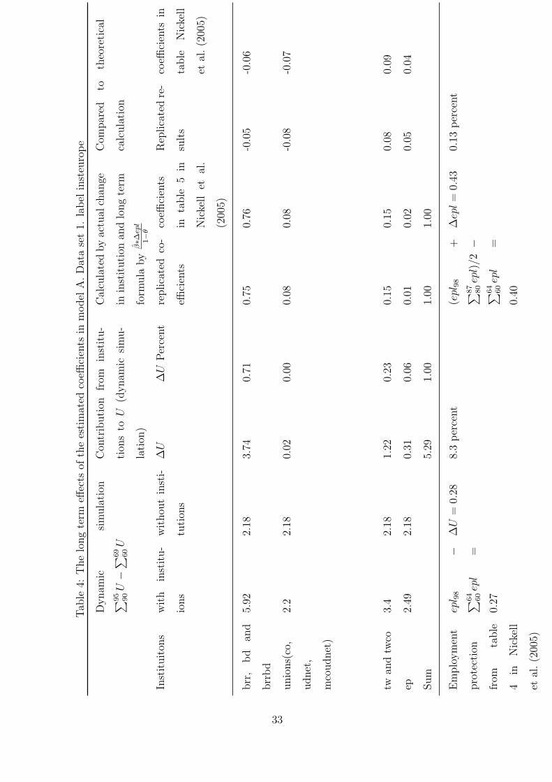
Nickell et al. (2005) claims that the variation in institutions accounts for 55 percent of
the increase in unemployment in Europe over the estimation period 1960 to 1995. The long
term effects of institutions are calculated in table 4. The table shows that our replication
implies that institutions accounts for 71 percent of the increase in unemployment in
Europe. This is consistent with the theoretical change, calculated by the long term effects
and actual change in data. (beregn ut i fra nick sine tabeller og koeff, lang tids effektene.)
The replication and the dynamic simulation on data set 1, imply that the values of
the replicated coefficients are slightly different from the estimated coefficients in Nickell
et al. (2005). But taking into consideration that all are within the original 90 percent
confidence intervals and the visual similarity in the dynamic simulation, the replication
of the results in Nickell et al. (2005) has been successful. The replicated results are used
as a comparison for further investigation when the data set is extended.
12

3.2 The model in table 5 in Nickell et al. (2005) is estimated on
data set 2
Nickell (2006) or the authors home page have data for institutional variables available up
to 2003. The macro variables from OECD (2007) are available up to 2007, although only
included to 2004. The extended time series are collected in a data base and is in what
follows denoted as data set 2. See appendix 6 for details.
The same procedure as in 3.1 for the replication, is now used to estimate the coefficients
on data set 2 over the period 1960 to 2004 for all 20 OECD countries. The results are
reported in this section.
The estimation results are given in table 5. The results are very different from table 1
and therefore also the original results in Nickell et al. (2005). In general both the effects of
institutional variables and shocks on unemployment are reduced. Several variables are no
longer significant. Three of the coefficients have changed sign: employment protection,
monetary shock and real interest rate. The variables were not significant in the first
regression though. The difference to Nickell et al. (2005) is also presented graphically
in figure 13. As mentioned in the discussion of the replication in section 3.1, the effect
of explanatory variables can be less stable if they are insignificant. This can be one
explanation to why these coefficients change dramatically when the data set is extended.
Section 3.3 will take a closer look at the specification, to see if revision of the data sets
or time extension causes the differences.
Even if the values of the estimated coefficients on data set 2 are somewhat different, it
is interesting to look at the models static simulation of unemployment and the dynamic
simulation. This should result in a bad fit of unemployment, at least for the period 1960
to 1995, but it seems that the new coefficients simulates the new data set very well over
that period, se figure 17. This can be because the model is too flexible because of time
dummies and country specific trends, in the sense that the model can capture actual
unemployment with any values of the estimated coefficients of the institutional and shock
variables. Or it could be that unemployment is quite stable, so that when all information
is used up to t− 1 unemployment to simulate unemployment this period t is not to hard
since adjustment by considering actual unemployment is made every period.
It is therefore necessary to look into the dynamic simulation. The dynamic simulation
13

of the estimated coefficients from table 5 are given in figure 3 and 4. skriv ut!
3.3 How much of the change in 3.2 is due to revisions?
This section reduces the time period in data set 2 to check wether the change in the
coefficients discovered in section 3.2 only are due to revisions of the data. The second
section looks at the performance of the former coefficients from data set 1, by simulateing
the unemployment rate for the new time period 1995 to 2004.
3.3.1 Is the change due to shocks
The figure of the dynamic simulation for the period 1960 to 2004, with zero shocks after
1995 is presented in figure 5. skriv ut!
3.3.2 Reduced time period on data set 2
The time period is reduced to detect if the coefficients in section 3.2 is due to the revision
of data or to the time extension. The former model in Nickell et al. (2005) is estimated
on data set 2, but only over the former available time period from 1960 to 1995.
The estimation results for period 1960 to 1995 on data set 2 are listed in table 6.
Five of the variables, benefit duration, union density, coordination and taxes, no longer
significant effect unemployment. The effect of employment protection is reduced, the
coefficient is nearly zero and not significant. Real interest rate has changed sign, but is
not significant. The change in the estimated coefficients compared to the original results
in Nickell et al. (2005) is presented in figure 14. The change in the values of the coefficients
indicates that the former values of coefficients are not very robust even to small changes
in the data set, i.e. to the revisions of the time series.
It seems that some of the difference is due to the new updated time series, and some
of the difference is due to the extended time period.
3.4 Estimation of model 5 in Nickell et al. (2005) on data set 3
The results are presented in table 8 and 7.
14

3.5 The effect of the specification of the error term Nickell et al.
(2005). Data set 1.
Equation (1) contain: the lagged endogenous variable, several explanatory variables, the
error term and the time and country dummies. The goal of an econometric specification
like equation (1) is to extract some homogenous effects of the included variables. This
section take a closer look at the econometric specification.
3.5.1 Error term
In the model estimated on equation 1 the error term is assumed to be heteroscedastic and
autocorrelated. The assumptions are expressed by equation 2.
uit = ρiui,t−1 + εit (2)
where εit is white noise. ρi is estimated for every country i by a iteration process.
The choice of this process for the error term where justified by a rejection of the joint
hypothesis ρi = 0 for all i, i.e. countries in the panel.
The coefficient of the lagged error term is unknown and has to be jointly estimated
with the coefficients. Table 5 lists the estimated country specific autocorrelation ρi. The
table shows great variation in ρi from -1.28 up to 3.18.
The estimation method assumes that the process in equation (2) is stationary, i.e.
|ρ| < 1. As seen from table 5 this is not the case for Japan, New Zealand and Portugal.
This means that the effect of the error term to unemployment increases over time. New
Zealand has positive autocorrelation in the error term. This means that unemployment
will increase or decrease steadily over time. Japan and Portugal have negative autocor-
relation in the error term. This means that the error term in one period will increase
unemployment but decrease unemployment in the next period. The positive and the
negative effect of the error term to unemployment will increase over time.
What are the effect of non-stationarity on the coefficients on the estimation method?
The effects are illustrated by a dynamic simulation in the next section.
15
3.5.2 Dynamic simulation, equation (1) is rewritten
As described in Nickell et al. (2005) the included country dummies, time dummies, country
specific trends and the lagged dependent variable, ”...are to ensure that the estimated
coefficients are not distorted by omitted trended variables in each country or common
shocks.”.
This means that the estimated coefficients in table 1 expresses the influence of the
included variables on unemployment regardless of the country considered.
The above reasoning depends on that the specification of the model is true. Equation
(1) can be rewritten to illustrate the effect of the heterogenous lagged error term on the
included variables. This requires four steps. Start by making a simplification of equation
(1) as:
Uit = θUi,t−1 + βXit + αYit + γ1t + γ2i + γ3iTt + uit (3)
where X is a vector consisting of the institutional variables and the interaction terms
in equation (1). The vector β contains the coefficients corresponding to the institutional
variables and the interaction terms in vector X. The shocks are collected in vector Y
with the coefficients in α.
Second, equation 3 also holds for period t−1. This equation contains the lagged error
term, ui,t−1, see equation 4.
Ui,t−1 = θUi,t−2 + βXi,t−1 + αYi,t−1 + γ1t−1 + γ2i + γ3iTt−1 + ui,t−1 (4)
Third, reorganize and insert the expression for ui,t−1 in equation 2. This gives the
following expression in equation 5:
uit = ρi[Ui,t−1 − (θUi,t−2 + βXi,t−1 + αYi,t−1 + γ1t−1 + γ2i + γ3iTt−1)] + εit (5)
Finally insert 5 in equation 3. This gives
Uit = θUi,t−1 + βXit + αYit + γ1t + γ2i + γ3iTt
+ρi ∗ [Ui,t−1 − (θUi,t−2 + βXi,t−1 + αYi,t−1 + γ1t−1 + γ2i + γ3iTt−1)] + εit(6)
16

Equation 6 has a white noise error term, εit. The equation can be organized as follows
in equation 7:
Uit = (θ + ρi)Ui,t−1 − ρiθUi,t−2 + β(Xit − ρiXi,t−1) + α(Yit − ρiYi,t−1)
+(γ1t − ρiγ1t−1) + (1 − ρi)γ2i + (γ3iTt − ρiγ3iTt−1) + εit (7)
Equation 7 shows that the process for the error term effects the estimated coefficients
of both the lagged endogenous variable and the exogenous variables included in the model.
The the estimated coefficient of the lagged endogenous variable, θ in table 1, is heteroge-
nous if the coefficient is adjusted by the effect of the lagged heteroscedastic autocorrelated
error term, ρi.
A dynamic simulation by equation 7 will illustrate also how the process for the specified
error term affects unemployment. This is illustrated in figure 15 and 16. The dynamic
simulation of the countries in figure 15 illustrates a similar pattern as the previous figures
in figure 10. As can be seen from figure 16 unemployment in New Zealand decreases
rapidly. For Japan and Portugal are there an negative autocorrelation. This means that
unemployment one period will increase with the error term, and the next decrease with
the error term. The positive and negative effects will increase over time, this is typically
the case for Portugal as illustrated in figure 3.
The figures illustrates that the model is not stationary when the error term is consid-
ered. The non stationarity can also be calculated by the 2. order differential equation in
equation 7. If the values of the last three columns of table 5 are greater than zero, will
the 2. order differential equation 7 will be stable. As seen from the table Japan, New
Zealand and Portugal have values lower than zero and are consistent with the previous
findings. empirical strategy
3.6 Some different specifications of the model.
Nickell et al. (2005) argue that this specification of the error term is correct since they
can not reject that ρ = 0 under an LM test, where χ(1) = 77.3. This test is however not
reliable when you include the lagged endogenous variable.
Arelleano bond :
17

The estimated coefficients of equation (1) are not consistent since both the lagged en-
dogenous variable and country specific effects appears in the same equation. The specified
process, Psar1, means that every error term has an estimated parameter and that L.U r is
correlated with the error term. This is normally handled by a procedure called Arelleano
bond.
Transformation:
Multiply both sides by the factor (1 − L)Ut where L is the lagged operator. Estimate on
this model. But how to account for the lagged error term.
3.6.1 Error term and graphical plot, not ready, any point?
Should residuals be heteroscedastic and autocorrelated?
A graphical plot of the error term, can we exclude the assumptions or include Ui,t−2
in equation?
4 Previous critique of Nickell et al. (2005)
Summarize the main critique of empirical papers trying to explain unemployment by
Baker et al. (b), Baker et al. (a), Howell et al. (2007) and also by Bassanini and Duval
(2006). Especially are the two latter a critique of Nickell et al. (2005). How trustworthy
are the results of Nickell et al. (2005)? This section looks at the other critiques and
summarizes the main findings.
Main critique:
Baker et al. (a) chapter 3, discusses an early version of Nickell et al. (2005). They claim
that the time effect trough the lagged endogenous variable are far to high to be reasonable.
For instance they claim that unemployment would have been negative if institutions where
hold constant throughout the period. One could question this remark, due to the fact
that time effects are not significant. The level of time effects in the model of Nickell et al.
(2005) should therefore be interpreted with care.
Indexes in themselves:
The indexes used in Nickell et al. (2005) are employment protection, benefit replacement
ratio, benefit duration, union density, taxes and coordination. There are several objections
18

to these indexes.
First of all it can be argued that these indexes not necessarily operate only in one
direction. For instance a higher coordination level can imply lower wage claims if the
level is above a certain level, see for instance ?. This is the famous results of the hump
shaped wage claims in the level of coordination, where medium level of coordination
results in highest wage clams. The low and the high coordination levels results in low
wage claims. This is also related to union density, and the insider outsider theory of wage
setting. Wage setters that covers the whole economy will according to the theory care for
unemployment levels. On the other hand will unions that only are responsible, only care
for parts of the economy in wage setting, care less of unemployment levels and more of
wage growth.
Further, employment protection can lead to lower unemployment in recessions. This
will be the case if employment protection makes employers more cautiously in hiring
workers in both recessions and in high growth periods. If unemployment benefits causes
workers to take more risk because they are less risk averse (benefits ensures the downside),
this can result in less unemployment because workers are more spread and actually result
in higher productivity growth.
Taxes and unemployment could be questioned according to Baker et al. (a). They point
out the between country variation, for instance high tax and low unemployment rate in
Sweden and low tax and high unemployment in Spain, implies that the relationship is not
clear.
The last thing to remember is that the causality between the indexes and unemploy-
ment are not obvious. The causality argument is also supported by Baker et al. (a).
The above arguments are made to see that it is not obvious that all indexes included
in Nickell et al. (2005) should have the sign achieved from the estimation of equation (1)
as listed in table 1.
Indexes are collected every 2. or 5th year, used as annual observations:
Wrong source of indexes:
The time series used in Nickell et al. (2005) are previously discussed, see for instance
Kenworthy (2001), Belot and van Ours (2004) and Baker et al. (b). Summarize.
19

5 Concludes
References
Baker, Dean, Glyn, Andrew, Howell, R. David, Schmitt, and John. 3.. labor market
institutions and unemployment: Assessment of the cross-country evidence. Fighting
Unemployment , 72–119.
Baker, Dean, Glyn, Andrew, Howell, R. David, Schmitt, and John. 3.. labor market
institutions and unemployment: The failure of the empirical case for deregulation.
Center for Economic and Policy Research 1611 Connecticut Avenue, NW Suite 400
Washington, DC 20009 , 72–119.
Bassanini, A. and R. Duval (2006, June). Employment patterns in oecd countries: Re-
assessing the role of policies and institutions.
Belot, M. and J. C. van Ours (2004). Does the recent success of some oecd countries in
lowering their unemployment rates lie in the clever design of their labor market reforms?
Oxford Economic Papers 56 (4), 621+.
Howell, D., D. Baker, A. Glyn, and J. Schmitt (2007). Are protective labor market
institutions at the root of unemployment? a critical review of the evidence. Capitalism
and Society 2 (1), 1.
Kenworthy, L. (2001). Wage-setting measures: A survey and assessment. World poli-
tics 54 (1), 57–98.
Layard, R., S. Nickell, and R. Jackman (1991). Unemployment: Macroeconomic Perfor-
mance and the Labour Market. Oxford University Press, USA.
Nickell, S., L. Nunziata, and W. Ochel (2005). Unemployment in the oecd since the 1960s:
What do we know? The Economic Journal (115), 1–27.
Nickell, W. (2006, November). The cep-oecd institutions data set (1960-2004).
OECD (2007). Oecd. Oecd .
20
List of Figures
1 Actual and static simulation of unemployment rate. Coefficients for simu-
lated unemployment from table 1. Time period 1960 to 2004. label predict1 24
2 Actual and static simulated unemployment rate. Coefficients for simulated
unemployment from table 1. Shocks are zero after 1995. Time period 1995
to 2004. label predict2 . . . . . . . . . . . . . . . . . . . . . . . . . . . . . 25
3 Dynamic simulation of unemployment rate and actual unemployment. Co-
efficients from table 1. Simulation period 1960 to 2004. Simulation on data
set 2. label dynsim2 . . . . . . . . . . . . . . . . . . . . . . . . . . . . . . 26
4 Dynamic simulation of unemployment rate and actual unemployment. Co-
efficients from table 1. Simulation period 1995 to 2004. label dynsim3 . . . 27
5 Dynamic simulation of unemployment rate and actual unemployment. Co-
efficients from table 1. Shocks are set to zero after 1995. label dynsim4 . . 28
6 Dynamic simulation of unemployment rate and actual unemployment. Co-
efficients from table 1. Institutions are constant. label dynsim5 . . . . . . . 29
7 The replicated coefficients on data set 1 (model A in table 1) compared
with the coefficients in Nickell et al. (2005). label nick reg1a . . . . . . . . 38
8 Model B in table 1 relative to model A. Only the number of time dummies
differ. Data set 1. label nick reg1b . . . . . . . . . . . . . . . . . . . . . . 38
9 The country specific trend, time dummies and country specific effects.
Model A and data set 1 relative to the original results in Nickell et al.
(2005). label nick reg1aa . . . . . . . . . . . . . . . . . . . . . . . . . . . . 39
10 Dynamic simulation of the coefficients estimated on data set 1 over the
years 1960 to 1995. label dynsim1a . . . . . . . . . . . . . . . . . . . . . . 40
11 Dynamic simulation of the coefficients estimated on data set 1 over the
years 1960 to 1995. With and without variation in institutions. label
dynsim1b . . . . . . . . . . . . . . . . . . . . . . . . . . . . . . . . . . . . 41
12 Dynamic simulation of the coefficients estimated on data set 1 over the
years 1960 to 1995. Excluding variation in one by one institution. label
dynsim1c . . . . . . . . . . . . . . . . . . . . . . . . . . . . . . . . . . . . 42
21

13 Estimation of equation (1) on data set 2, compared with the coefficients in
Nickell et al. (2005). Period 1960-2004. label reg1a . . . . . . . . . . . . . 43
14 Estimation of equation (1) on data set 2, compared with the coefficients in
Nickell et al. (2005). Time period 1960-1995 . . . . . . . . . . . . . . . . . 43
15 The transformed equation 7. Model A in 1. Data set 1. label dynsim2a . . 45
16 The transformed equation 7. Model A in 1. Data set 1. label dynsim2b . . 46
17 Static simulation of model for unemployment in Nickell et al. (2005) over
the years 1960 to 2004. Estimated coefficients from table 5 are used in the
simulation. . . . . . . . . . . . . . . . . . . . . . . . . . . . . . . . . . . . . 47
18 Dynamic simulation and actual unemployment. Coefficients in table 5 over
the years 1960 to 2004. Simulation and estimation on data set 2. . . . . . . 48
19 Dynamic simulation with and without the effect of institutions to unem-
ployment. Coefficients in table 5 over the years 1960 to 2004. Simulation
and estimation on data set 2. . . . . . . . . . . . . . . . . . . . . . . . . . 49
20 Actual unemployment. Data set 2 over the years 1960 to 2007. label ur . . 54
List of Tables
1 Model 1 is the results in table 5 in Nickell et al. (2005). Model A is the
replication of model 1 on data set 1. Model B is the replication, but pools
the time dummies over the years 1966 and 1967 with the former periods
1960 to 1966. label t1emp . . . . . . . . . . . . . . . . . . . . . . . . . . . 30
2 Model A, replication like Model A in table 1. Model B, the same explana-
tory variables as Model A, but pools ρ, i.e. no heteroscedastic lagged error
term. Model C, the same as Model B, but the lagged error term ρ, follows
a calc process. . . . . . . . . . . . . . . . . . . . . . . . . . . . . . . . . . . 31
3 The error term and stability restrictions. Data set 1. label stabrho . . . . . 32
4 The long term effects of the estimated coefficients in model A. Data set 1.
label insteurope . . . . . . . . . . . . . . . . . . . . . . . . . . . . . . . . . 33
5 Model A is a replication of model 1 given in table 5 in Nickell et al. (2005)
on data set 2. Time period 1960-2004. label t2emp . . . . . . . . . . . . . 34
22

6 Model 1 is a replication of model 1 given in table 5 in Nickell et al. (2005)
on data set 2. Time period 1960-1995. label t3emp . . . . . . . . . . . . . 35
7 Replication of model 1 given in table 5 in Nickell et al. (2005) on data set
3. Time period 1960 until 1995. label t5emp . . . . . . . . . . . . . . . . . 36
8 Replication of model 1 given in table 5 in Nickell et al. (2005) on data set
3. Time period 1960 until 2004. label t7emp . . . . . . . . . . . . . . . . . 37
9 Unemployment as Nickell et al. (2005) has presented the data, data set 2 . 50
10 Macrovariables . . . . . . . . . . . . . . . . . . . . . . . . . . . . . . . . . 51
11 Constructed variables . . . . . . . . . . . . . . . . . . . . . . . . . . . . . . 52
12 Institutional variables . . . . . . . . . . . . . . . . . . . . . . . . . . . . . . 53
23

Figure 1: Actual and static simulation of unemployment rate. Coefficients for simulated
unemployment from table 1. Time period 1960 to 2004. label predict1
24

Figure 2: Actual and static simulated unemployment rate. Coefficients for simulated
unemployment from table 1. Shocks are zero after 1995. Time period 1995 to 2004. label
predict2
25
Figure 3: Dynamic simulation of unemployment rate and actual unemployment. Coef-
ficients from table 1. Simulation period 1960 to 2004. Simulation on data set 2. label
dynsim2
26

Figure 4: Dynamic simulation of unemployment rate and actual unemployment. Coeffi-
cients from table 1. Simulation period 1995 to 2004. label dynsim3
27

Figure 5: Dynamic simulation of unemployment rate and actual unemployment. Coeffi-
cients from table 1. Shocks are set to zero after 1995. label dynsim4
28

Figure 6: Dynamic simulation of unemployment rate and actual unemployment. Coeffi-
cients from table 1. Institutions are constant. label dynsim5
29

Table 1: Model 1 is the results in table 5 in Nickell et al. (2005). Model A is the replication
of model 1 on data set 1. Model B is the replication, but pools the time dummies over
the years 1966 and 1967 with the former periods 1960 to 1966. label t1emp
Model 1 in table 5 in Nickell et al. (2005)
b t
L.ur 0.86 48.5
epl 0.15 0.9
brr 2.21 5.4
bd 0.47 2.5
brrbd 3.75. 4.0
codudnet -6.98 6.1
cotw -3.46 3.3
D.udnet 6.99 3.2
co -1.01 3.5
tw 1.51 1.7
lds -23.6 10.4
tfp -17.9 14.1
d2m 0.23 0.9
rirl 1.81 1.6
tts 5.82 3.3
obs 600
time periods
numb groups 20
min groups 12
max groups 33
avg groups 31.2
coef 85
est cov 20
est autocorr 20
log like -599.55
autocorr
Source:Nickell et al. (2005)
Model A Model B
b t b t
L.ur 0.86 47.61 0.86 47.51
ep 0.11 0.68 0.12 0.70
brr 2.33 5.61 2.32 5.61
bd 0.45 2.27 0.46 2.30
mbrrbd 3.72 3.75 3.75 3.78
mcoudnet -7.04 -6.14 -7.05 -6.14
mcotw -3.10 -2.98 -3.09 -2.97
D.udnet 6.55 3.16 6.55 3.16
co -0.90 -3.16 -0.89 -3.12
tw 1.54 1.77 1.53 1.76
lds -22.08 -10.19 -21.81 -10.11
tfphpc -17.29 -13.70 -17.28 -13.74
d2ms 0.23 0.98 0.24 1.02
rirl 2.22 1.93 2.20 1.91
tts 5.44 3.10 5.44 3.10
obs 599 599
time periods 33 33
numb groups 20 20
min groups 12 12
max groups 33 33
avg groups 29.95 29.95
coef 85 83
estimated cov 20 20
estimated autocorr 20 20
log likelihood -604.72 -598.52
estimated autocorr 43594 43409
Source: Data set 1
30

Table 2: Model A, replication like Model A in table 1. Model B, the same explanatory
variables as Model A, but pools ρ, i.e. no heteroscedastic lagged error term. Model C,
the same as Model B, but the lagged error term ρ, follows a calc process.
Model A Model B Model C
b t b t b t
L.ur .8635487 47.60779 .7744939 32.08049 .7924479 33.6793
ep .1108613 .6767546 -.0127239 -.0582341 -.2027108 -.7113987
brr 2.327419 5.612366 2.198545 4.124974 2.339849 3.969217
bd .4511384 2.271153 .5226619 2.195521 .5441488 1.616523
mbrrbd 3.722513 3.75492 5.098122 4.159219 4.772874 3.387187
mcoudnet -7.036643 -6.137761 -5.707323 -4.072997 -4.861822 -3.028288
mcotw -3.098725 -2.978097 -3.689448 -2.859484 -2.550337 -1.704073
D.udnet 6.550333 3.15664 2.265205 1.287162 3.42791 1.73165
co -.9015665 -3.155782 -.6419443 -1.743556 -.6871283 -2.091191
tw 1.542205 1.774337 .6883075 .6362186 .789933 .6849612
lds -22.0755 -10.18768 -15.90552 -9.945486 -18.61467 -9.706006
tfphpc -17.28824 -13.70104 -15.97227 -12.78158 -18.55733 -12.61648
d2ms .2342279 .9827281 .3667688 2.31497 .46535 2.468598
rirl 2.224254 1.928584 1.62581 1.47075 1.532278 1.27637
tts 5.444384 3.097698 4.128078 2.683663 3.283862 2.032268
obs 599 599 599
time periods 33 33 33
numb groups 20 20 20
min groups 12 12 12
max groups 33 33 33
avg groups 29.95 29.95 29.95
coef 85 85 85
estimated cov 20 20 1
estimated autocorr 20 20 20
log likelihood -604.7176 -385.3741 -434.1662
estimated autocorr 43593.92 28811.02 20096.14
Source: Data set 1
31

Table 3: The error term and stability restrictions. Data set 1. label stabrho
Stability
Country rhoi a1 a2 real root if > 0 1 + a1 + a2 > 0 1 − a1 + a2 > 0 1 − a2 > 0
Australia 0.46 -1.33 0.40 0.04 0.07 2.72 0.60
Austria -0.15 -0.72 -0.13 0.26 0.16 1.59 1.13
Belgium -0.59 -0.27 -0.51 0.53 0.22 0.76 1.51
Canada -0.30 -0.56 -0.26 0.34 0.18 1.30 1.26
Denmark -0.48 -0.38 -0.42 0.45 0.20 0.96 1.42
Finland -0.97 0.11 -0.84 0.84 0.27 0.06 1.84
France 0.28 -1.14 0.24 0.09 0.10 2.38 0.76
Germany -0.39 -0.48 -0.33 0.39 0.19 1.14 1.33
Ireland -0.25 -0.61 -0.22 0.31 0.17 1.39 1.22
Italy -0.65 -0.22 -0.56 0.57 0.23 0.66 1.56
Japan -1.11 0.25 -0.96 0.97 0.29 -0.20 1.96
Netherlands -0.77 -0.09 -0.66 0.67 0.24 0.43 1.66
New Zealand 3.18 -4.04 2.73 1.35 -0.31 7.77 -1.73
Norway -0.53 -0.33 -0.46 0.49 0.21 0.87 1.46
Portugal -1.28 0.42 -1.10 1.15 0.32 -0.52 2.10
Spain -0.97 0.10 -0.83 0.83 0.27 0.07 1.83
Sweden -0.38 -0.48 -0.33 0.39 0.19 1.15 1.33
Switzerland -0.67 -0.19 -0.58 0.59 0.23 0.61 1.58
United Kingdom -0.41 -0.45 -0.35 0.40 0.19 1.10 1.35
United States -0.38 -0.48 -0.33 0.39 0.19 1.15 1.33
32
Tab
le4:
The
long
term
effec
tsof
the
esti
mat
edco
effici
ents
inm
odel
A.D
ata
set
1.la
bel
inst
euro
pe
Dynam
icsi
mula
tion
∑ 95 90U−
∑ 69 60U
Con
trib
uti
onfr
omin
stit
u-
tion
sto
U(d
ynam
icsi
mu-
lation
)
Cal
cula
ted
by
actu
alch
ange
inin
stit
uti
onan
dlo
ng
term
form
ula
by
β̂∗∆
epl
1−
θ
Com
par
edto
theo
reti
cal
calc
ula
tion
Inst
ituit
ons
wit
hin
stit
u-
ions
wit
hou
tin
sti-
tuti
ons
∆U
∆U
Per
cent
replica
ted
co-
effici
ents
coeffi
cien
ts
inta
ble
5in
Nic
kell
etal
.
(200
5)
Rep
lica
ted
re-
sult
s
coeffi
cien
tsin
table
Nic
kell
etal
.(2
005)
brr
,bd
and
brr
bd
5.92
2.18
3.74
0.71
0.75
0.76
-0.0
5-0
.06
unio
ns(
co,
udnet
,
mco
udnet
)
2.2
2.18
0.02
0.00
0.08
0.08
-0.0
8-0
.07
twan
dtw
co3.
42.
181.
220.
230.
150.
150.
080.
09
ep2.
492.
180.
310.
060.
010.
020.
050.
04
Sum
5.29
1.00
1.00
1.00
Em
plo
ym
ent
pro
tect
ion
from
table
4in
Nic
kell
etal
.(2
005)
epl 9
8−
∑ 64 60ep
l=
0.27
∆U
=0.
288.
3per
cent
(epl
98
+∑ 87 8
0ep
l)/2
−∑ 64 6
0ep
l=
0.40
∆ep
l=
0.43
0.13
per
cent
33

Table 5: Model A is a replication of model 1 given in table 5 in Nickell et al. (2005) on
data set 2. Time period 1960-2004. label t2emp
(1)
U r p
b t
L.U r p 0.91 67.91
epl nic1 ext 0.51 3.52
brr nic ext 0.80 2.89
bd nic ext 0.03 0.24
mbrrbd ext 1.55 2.51
mcodudnet ext -3.41 -4.86
mcodtw ext -2.64 -2.56
D.udnet vis nic1 ext 1.51 0.79
co nic ext -0.21 -0.99
tw nic1 ext 2.28 2.81
lds ext -22.24 -9.12
Dprod hp ext -8.21 -8.42
D2m ext 0.38 1.11
RIRL ext -2.00 -2.09
TTS ext 7.69 5.01
obs 873
time periods 45
numb groups 20
min groups 33
max groups 45
avg groups 43.65
coef 92
est cov 20
est autocorr 20
log like -889.92
autocorr 62110
34

Table 6: Model 1 is a replication of model 1 given in table 5 in Nickell et al. (2005) on
data set 2. Time period 1960-1995. label t3emp
(1)
U r p
b t
L.U r p 0.91 47.75
epl nic1 ext 0.10 0.41
brr nic ext 1.43 3.95
bd nic ext 0.31 1.67
mbrrbd ext 1.27 1.59
mcodudnet ext -4.39 -4.39
mcodtw ext -3.38 -2.46
D.udnet vis nic1 ext -0.30 -0.14
co nic ext -0.08 -0.28
tw nic1 ext 0.56 0.63
lds ext -15.62 -9.51
Dprod hp ext -11.87 -12.21
D2m ext 0.22 0.75
RIRL ext -0.46 -0.68
TTS ext 10.53 6.77
obs 633
time periods 33
numb groups 20
min groups 21
max groups 33
avg groups 31.65
coef 83
est cov 20
est autocorr 20
log like -652.85
autocorr 1332912
35

Table 7: Replication of model 1 given in table 5 in Nickell et al. (2005) on data set 3.
Time period 1960 until 1995. label t5emp
(1)
U r p
Coef. t
L.U r p 0.889 45.214
epl back p -0.428 -2.962
ibrr p 1.023 2.967
ibd p -0.107 -0.626
mibrrbd p 0.785 1.004
micodudnet p -2.833 -6.677
mcodtw p 0.011 1.856
D.iudnet bd p 0.701 0.431
icoord p 0.180 2.684
TW -0.002 -0.261
lds p -14.992 -8.665
Dprod hp p -11.210 -11.994
D2m p 0.105 0.372
RIRL p -0.802 -1.176
TTS p 9.846 6.218
obs 633.000
time periods 33.000
numb groups 20.000
min groups 21.000
max groups 33.000
avg groups 31.650
coef 83.000
est cov 20.000
est autocorr 20.000
log like -653.156
autocorr 1.25e+06
36

Table 8: Replication of model 1 given in table 5 in Nickell et al. (2005) on data set 3.
Time period 1960 until 2004. label t7emp
(1)
U r p
Coef. t
L.U r p 0.872 56.310
epl back p -0.234 -1.976
ibrr p 1.226 4.014
ibd p -0.038 -0.242
mibrrbd p 1.520 2.203
micodudnet p -2.444 -6.833
mcodtw p 0.009 1.736
D.iudnet bd p 1.681 1.146
icoord p 0.124 2.106
TW -0.004 -0.467
lds p -11.487 -8.696
Dprod hp p -10.931 -13.395
D2m p -0.358 -1.521
RIRL p -1.103 -1.855
TTS p 9.031 6.414
obs 755.000
time periods 45.000
numb groups 20.000
min groups 24.000
max groups 45.000
avg groups 37.750
coef 94.000
est cov 20.000
est autocorr 20.000
log like -755.769
autocorr 2.88e+06
37

Figure 7: The replicated coefficients on data set 1 (model A in table 1) compared with
the coefficients in Nickell et al. (2005). label nick reg1a
Figure 8: Model B in table 1 relative to model A. Only the number of time dummies
differ. Data set 1. label nick reg1b
38

Figure 9: The country specific trend, time dummies and country specific effects. Model
A and data set 1 relative to the original results in Nickell et al. (2005). label nick reg1aa
39

Figure 10: Dynamic simulation of the coefficients estimated on data set 1 over the years
1960 to 1995. label dynsim1a
40
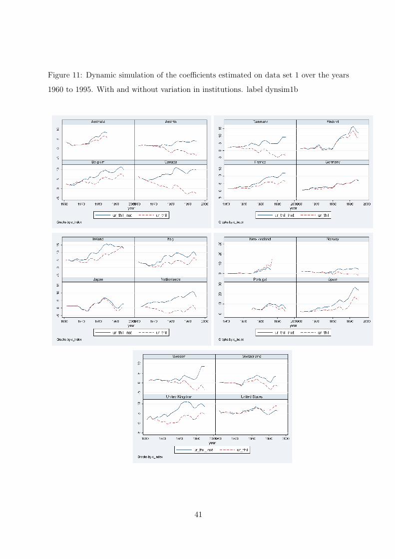
Figure 11: Dynamic simulation of the coefficients estimated on data set 1 over the years
1960 to 1995. With and without variation in institutions. label dynsim1b
41

Figure 12: Dynamic simulation of the coefficients estimated on data set 1 over the years
1960 to 1995. Excluding variation in one by one institution. label dynsim1c
42
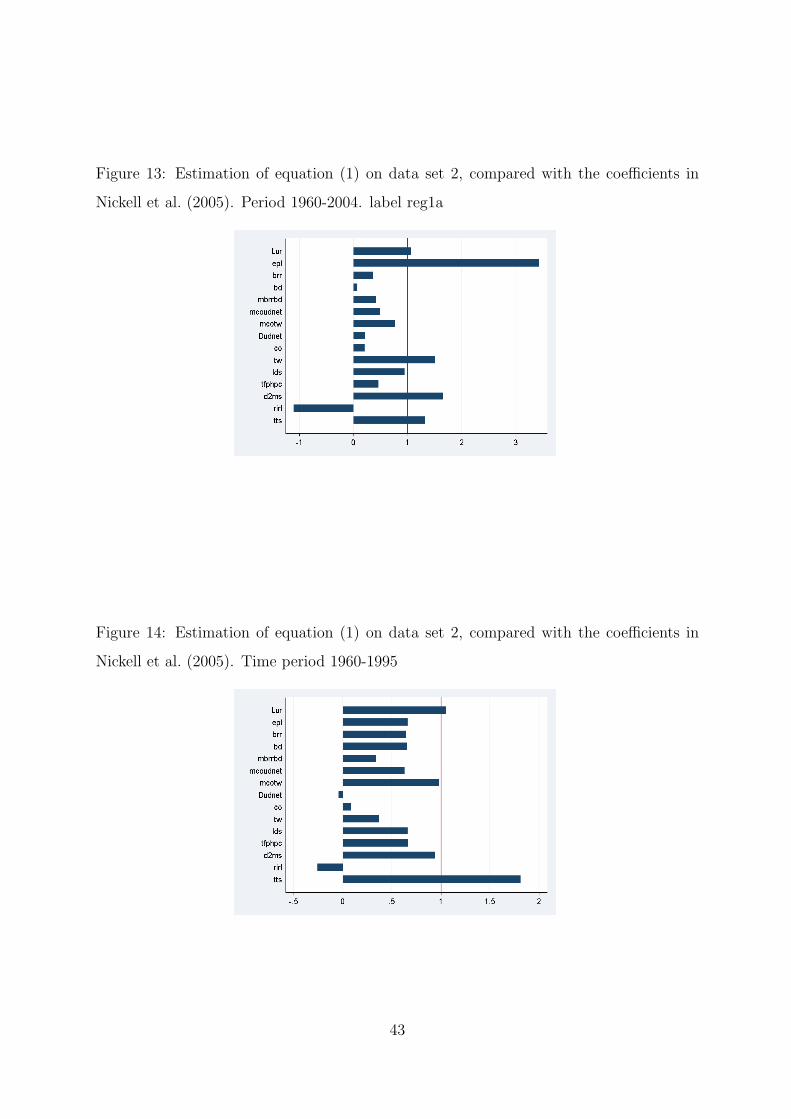
Figure 13: Estimation of equation (1) on data set 2, compared with the coefficients in
Nickell et al. (2005). Period 1960-2004. label reg1a
Figure 14: Estimation of equation (1) on data set 2, compared with the coefficients in
Nickell et al. (2005). Time period 1960-1995
43

6 Background Data
44

Figure 15: The transformed equation 7. Model A in 1. Data set 1. label dynsim2a
45

Figure 16: The transformed equation 7. Model A in 1. Data set 1. label dynsim2b
46

Figure 17: Static simulation of model for unemployment in Nickell et al. (2005) over the
years 1960 to 2004. Estimated coefficients from table 5 are used in the simulation.
47

Figure 18: Dynamic simulation and actual unemployment. Coefficients in table 5 over
the years 1960 to 2004. Simulation and estimation on data set 2.
48

Figure 19: Dynamic simulation with and without the effect of institutions to unemploy-
ment. Coefficients in table 5 over the years 1960 to 2004. Simulation and estimation on
data set 2.
49

Tab
le9:
Unem
plo
ym
ent
asN
icke
llet
al.(2
005)
has
pre
sente
dth
edat
a,dat
ase
t2
countr
yY
r6064
Yr6
572
Yr7
379
Yr8
08
7Y
r8895
Yr9
6103
Yr1
04107
Aust
ralia
2.57
1.88
4.64
7.66
8.43
7.10
5.01
Aust
ria
1.87
1.50
1.32
3.11
4.67
5.30
5.82
Bel
gium
1.41
1.40
4.23
9.58
8.05
8.22
8.13
Can
ada
6.12
4.79
6.98
9.84
9.53
7.99
6.64
Den
mar
k1.
601.
233.
776.
687.
494.
984.
59
Fin
land
1.38
2.37
4.14
5.17
10.8
510
.93
8.21
Fra
nce
1.51
2.31
4.46
9.05
10.4
410
.44
9.63
Ger
man
y0.
460.
571.
835.
105.
927.
748.
72
Gre
ece
.3.
192.
086.
398.
3510
.94
10.2
5
Icel
and
.1.
571.
211.
483.
562.
942.
49
Irel
and
5.22
5.78
8.21
14.2
714
.90
6.65
4.38
Ital
y3.
484.
194.
877.
969.
9010
.27
7.82
Jap
an1.
311.
211.
832.
522.
464.
494.
16
Net
her
lands
0.56
1.08
3.20
7.50
6.00
3.85
4.36
New
Zea
land
0.11
0.37
0.74
3.95
8.14
6.00
4.20
Nor
way
1.95
1.55
1.74
2.44
5.13
3.82
4.20
Por
tuga
l.
3.11
5.63
8.23
5.48
5.34
7.49
Spai
n1.
812.
194.
2214
.51
15.0
012
.97
9.26
Sw
eden
1.65
2.01
1.99
2.75
4.62
5.72
5.07
Sw
itze
rlan
d0.
200.
000.
280.
612.
153.
283.
98
UK
3.08
3.49
4.81
10.4
48.
776.
005.
02
Unit
edSta
tes
5.82
4.51
6.51
7.75
6.16
4.95
5.00
Tot
al2.
222.
253.
586.
687.
556.
816.
11
Sour
ce:
Z:/
StH
/vic
/fra
Z/d
oes
tny
data
/vr0
8/R
eplic
N/t
emp1
.dta
50

Table 10: Macrovariables
Variable Time series, OECD definition
YC Gross Domestic Product (Market prices), Value
YQ V Gross Domestic Product (Market prices), Volume
Cp V Private Consumption, Volume
I V Total Fixed Investment (Excl Stockbuilding), Volume
Ig V Government Investment, Volume
NAWRU nawru
Ip V Private Fixed Investment (Excl Stockbuilding), Volume
Iph V Private investment in Housing 2, Volume
X V Exports Goods and Services, N.A. Basis, Volume
Pi d Import Price Goods and Services, Local Currency - deflator
Pgdp dm Deflator for GDP at Market Prices
CPI i Consumer Price Index
SUB Subsidies
TAXh Direct Taxes, Households
SSRG Social Security Contributions Received by Government
TAXind Indirect Taxes
IE Compensation of Employees
WAGE Wages and Salary
CRh Current Receipts Households
Cp Private Consumption, Household Account Basis
S r Saving Ratio
RW i Real Labour Cost
Wbus Wage Rate (Business Sector)
EPOP r Labour Force, Participation Ratio
L Labour Force, Total
N Total employment
U r Unemployment Rate
POP1564 Population, Total (15 and 64 years old, except USA, ESP, HUN, NZL, MEX see country’s notes)
M Money Stock
Is r Interest Rate, ShortTerm
Il r Interest Rate, LongTerm
MC V Imports of goods and services, value, local currency
Cg V Government consumption, volume
SBp V Stockbuilding private, volume
Source: OECD and others
51

Table 11: Constructed variables
Variable Constructed variables from time series data
t1 Employment tax rate
t2 Direct tax rate
t3 Indirect tax rate
TW Tax wedge
LABC Labour cost
infl Inflation rate
RIRL Real interest rate
prodhp Trade productivity
D2MS Acceleration in money supply
lds Labour demand shock
TTS Terms of trade shock
Dprod hp Deviations from labour productivity in the business sector
Average Hours Per Employee
Index of Relative Unit Labour Cost Manufacturing Sector, Common Currency
(Overall Competitiveness)
52

Table 12: Institutional variables
Variable Definition
BRR Average of brr66 and brr100. And brr66 is the average of r67a1-r67a4 and the same for brr100 OECD
brr67a1 Benefit replacement rate for workers with 66 percent of average earnings, first year, OECD (corresponds to brr66 in ? )
brr67a2 Benefit replacement rate for workers with 66 percent of average earnings, second and third year, OECD
brr67a4 Benefit replacement rate for workers with 66 percent of average earnings, fourth and fifth year, OECD
brr100a1 Benefit replacement rate for workers with average earnings, first year, OECD (corresponds to brr100 in ?)
brr100a2 Benefit replacement rate for workers with average earnings, second and third year, OECD
brr100a4 Benefit replacement rate for workers with average earnings, fourth and fifth year, OECD
bd66 Benefit duration for workers with 100 percent of average earnings, calculated
bd100 Benefit duration for workers with 66 percent of average earnings, calculated
iudnet Union density, OECD, interpolated
udnet nic1 Union density, Nickell (2006).
icentr Centralization, OECD, interpolated
cov Coverage, OECD
epl 1 Average employment protection (average of epl i and epl t), OECD table
epl 2 Average employment protection (average of epl i and epl t and epl c), OECD table
epl i Overall strictness of protection against (individual) dismissals, OECD table
epl c Overall strictness of regulation on collective dismissals, OECD table
epl t Overall strictness of regulation on temporary employment, OECD table
epl Overall employment protection, time series version from OECD
eplr Regular employment protection, time series version from OECD
eplt Temporary employment protection, time series version from OECD
ERTOT bo Average employment protection (sum of EP, FT and TWA), Belot and Ours
EP bo Protection open ended contracts, Belot and Ours
FT bo Protection fixed term contracts, Belot and Ours
TWA bo Protection temporary work agencies, Belot Ours
epl back Overall employment protection prolonged backwards via backcast by use of ERTOT bo from Belot and Ours
epl back 1 Employment protection open ended contracts, prolonged backwards via backcast by use of EP bo from Belot and Ours
icoord Coordination, OECD, interpolated
co back Coordination with backcast by use of Kenworthy
co ken Coordination, Kenworthys
ho Housing (percentage owner occupied), Oswald53

Figure 20: Actual unemployment. Data set 2 over the years 1960 to 2007. label ur
54