LayoutCalculations

FIRST EDITION : JANUARY 2012

SECOND EDITION : NOVEMBER 2016

Price `80/-

Layout

Calculations

Indian Railways Institute of Civil Engineering,Pune - 411001.

October 2016

Foreword to Second Edition

The knowledge of turnout geometry and layout is an essential pre-requisite for laying of new turnout, or improvement of existing layoutgeometry. A good layout results in improved riding quality as well asreduction in maintenance efforts. The calculations for Layout is notvery complex provided necessary information/data, and methodologyare available beforehand. This publication on layout calculation alsoincludes layout calculation for improved turnout structure like PSClayout on 60kg/ 52kg PSC curved switches with elaborated andimproved and legible diagrams. While laying out a turn out relevantprovisions of IRPWM and Schedule of Dimensions to be always keptin mind which are incorporated in the book for ready reference.

The software Programme developed by Shri M.S. Ekbote, ex. AM(Civil) Railway Board could be of immense help for calculations forvarious yard layouts connections, cross over etc. available at IRICENweb site.

I hope this book will extremely useful for field engineer forunderstanding in layout calculation and apply it for improvingreliability of assets, reduction in maintenance requirements as well asimproved riding quality.

October - 2016 N. C. ShardaDirectorIRICEN

Preface to Second Edition

The maintainability and riding quality over a turnout depends largelyon how accurately it is laid and maintained. It is a known fact that yardmay require various combinations of turnouts (i.e. switches, leads& crossings), with curves and straights, to transfer trains from onetrack to another or enable trains to cross other tracks. For satisfying thevarious geometrical features of the layouts, one has to perform varietyof trigonometric calculations .Understanding of Layout Calculations isnecessary, all possible problems and proposed solutions are greatlycovered in existing layout calculation book published by IRICEN.

This revised publication on layout calculation includes layoutcalculation for improved turnout structure like PSC layout on 60kg/52kg PSC curved switches with elaborated and improved and legiblediagrams by removing old 90lbs layouts. Further for laying out a turnout relevant provisions of IRPWM and Schedule of Dimensions to bealways kept in mind, are incorporated in the book for ready reference.

I am grateful to Shri N. C. Sharda, Director, IRICEN for giving me theopportunity for revising the contents and also for his encouragementand guidance from time to time for bringing out this publication.Thanks are also due to Shri Suresh Pakhare Professor (Track) IRICEN,now for checking the drafts and for giving his valuable suggestions. Iam thankful to faculty and staff of IRICEN who have contributedimmensely for this publication. Efforts taken by Shri Pravin Kotkar SI/T in correcting the draft and scrutinizing the manuscript are alsoappreciated.

Suggestions from readers to improve the contents are welcome and canbe sent to mail@iricen.gov.in which will be taken into account whilebringing future editions.

October - 2016 N. K. MishraAssociate Professor/Track

IRICEN

Foreword to First Edition

The maintainability and riding quality over a turnout depend largely onhow accurately it is laid and maintained. Deficiencies can be nipped inthe bud if adequate care is taken by laying turnouts accurately aftercarrying out layout calculations.

Layout calculations, as the name indicates, are the set of calculationsfor the various yard layouts so that the same can be correctly laid in thefield. Layout calculations become more important in case of yardremodelling or designing a new yard. These calculations are intricate innature and require considerable efforts on the part of field engineerswhich often get neglected due to other engagements in the field andtherefore, this item of work does not get proper attention.

Railway Engineers had been expressing the need for bringing out abook on ‘‘Layout Calculations’’ which was out of print since long.Special efforts have been taken to make this book more effective byincorporating colored drawings of the layouts developed by usingAutoCad software. Worked out examples on practical situationscommonly met with, have also been given for better understanding ofthis subject.

Another special feature of the book is the inclusion of a software onLayout Calculations, which had been developed by Shri M. S. Ekbote,Ex. AM(Civil Engineering), Railway Board, using Visual Basic withinteractive and user friendly interface.

I hope that this book on Layout Calculations will go a long way infulfilling the need of railway engineers for better designing and correctlaying of layouts.

Shiv KumarDirectorIRICEN

ii

Acknowledgement to First Edition

Subject of “Layout Calculations” is being covered in various coursesbeing held at IRICEN. In every course at IRICEN, trainee officers haveexpressed the need of a book on Layout Calculations as the earlierpublication had become out of print. Besides, several developments hadtaken place in the field of turnout such as PSC layouts. Considering therequirement of the field engineers, the entire book has been rewritten.Apart from the theory and illustrations the book contains several newfeatures such as coloured drawings, interpretations of trigonometricformulae and a software on Layout Calculations

We are very much grateful to Shri Abhay Kumar Gupta, Professor/Track -1 for the proof checking of the entire book.

We are also very much grateful to Shri M.S. Ekbote, Ex. AM(CivilEngineering), Railway Board, for his active support for rewriting thechapter on Scissors Cross-over and developing a Software Program onLayout Calculations which is available on a CD attached with this book.

Above all, the authors are very much grateful to Shri Shiv Kumar,Director, IRICEN for his encouragement and guidance.

Abhai Kumar Rai Praveen KumarProfessor/Works Professor/Computers

IRICEN IRICEN

iii

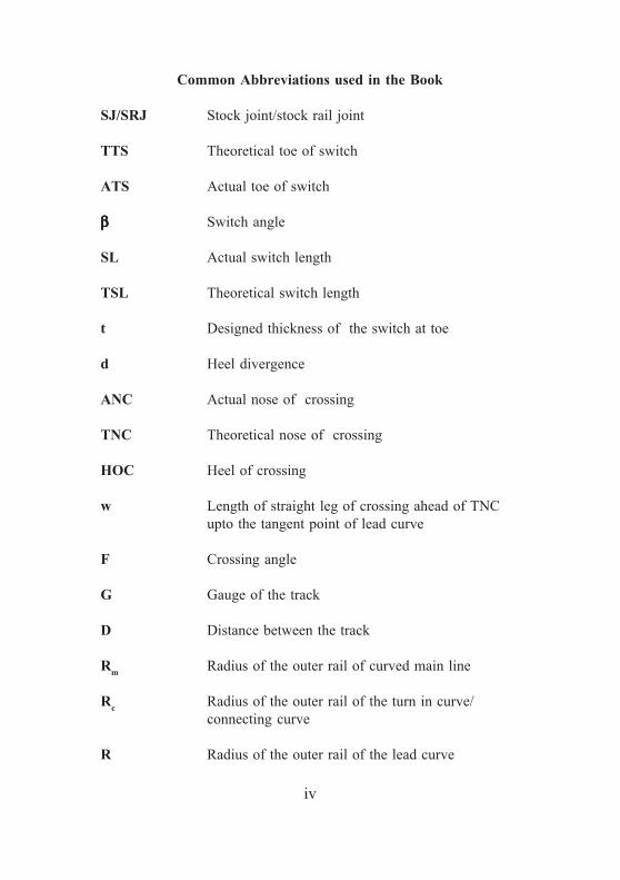
Common Abbreviations used in the Book

SJ/SRJ Stock joint/stock rail joint

TTS Theoretical toe of switch

ATS Actual toe of switch

βββββ Switch angle

SL Actual switch length

TSL Theoretical switch length

t Designed thickness of the switch at toe

d Heel divergence

ANC Actual nose of crossing

TNC Theoretical nose of crossing

HOC Heel of crossing

w Length of straight leg of crossing ahead of TNCupto the tangent point of lead curve

F Crossing angle

G Gauge of the track

D Distance between the track

Rm Radius of the outer rail of curved main line

Rc Radius of the outer rail of the turn in curve/connecting curve

R Radius of the outer rail of the lead curve

iv

OL Over all length of the layout

S Length of straight portion outside the turnout

A Distance from ‘SJ’ to the point of intersection in aturnout measured along the straight

B Distance from the point of intersection to the heelof crossing measured along the straight

K Distance from TNC of the crossing to the heel ofcrossing measured along the straight

v

CONTENTS

1. Turnouts 1

2. Lead and Radius of IRS Turnout 22

3. Connections to Diverging Tracks 30

4. Connections to Straight Parallel Tracks 41

5. Crossover Connection between Straight Parallel 57Tracks

6. Scissors Cross-Over between Straight Parallel Tracks 81

7. Crossovers between Non Parallel Straight Tracks 86

8. Connection between Curved Track to Parallel 89Curved Track or Divergent Straight Track

9. Crossover Connection between two Curved Parallel 117Tracks

10. Software on Layout Calculations 125

Table of Detailed Dimensions 133

vii

1

Figure 1.1: A Turnout

Chapter 1

Turnouts

1.0 Introduction

1.0 (a) - Turnouts provide the means by which a train may betransferred from one track to another track. To be more specific, as perORE report on Q.No. D.72, the term ‘Turnout’ means a layoutpermitting the passage of rolling stock on two or more routes from onecommon route. In its simplest form, i.e. where only two routes areinvolved, it consists of a pair of switches (one right hand and the otherleft hand) and a common crossing assembly ( composed of a commoncrossing, two wing rails and two check rails), together with lead railsconnecting the two routes. As desired, the crossing ensuresunobstructed flange way clearances for the wheels at the intersectionbetween the left hand rail of one route and the right hand rail of theother.

Turnouts are, therefore, the most sophisticated component of railwaytrack structure. To design and perfect different types of turnouts tomeet the varied requirements of operations has always been achallenging task for the permanent way engineer. Turnouts may takeoff from a straight track or a curved track.

A turnout has, therefore, three distinct portions (Fig 1.1);• Switch Assembly• Lead Assembly• Crossing Assembly

2

Main Dimensions of a turnout are as shown in Fig 1.2.

Figure 1.2: Main dimensions of a turnout

The switch assemblies in use on Indian Railways are classified purelybased on their geometry as shown below:

• IRS- Straight Switches (Fig 1.3)

Figure 1.3: Straight switches

3

• IRS- Partly Curved Switches (Fig 1.4)

Figure 1.4: Partly curved switches

• IRS-Curved Switches

The curved switches are further classified into the followingtypes:

• Non - Intersecting type (Fig 1.5a)

Figure 1.5a : Non- intersecting type

4

• Intersecting type (Fig 1.5b)

Figure 1.5b : Intersecting type

• Tangential type (Fig 1.5c)

Figure 1.5c : Tangential type

5

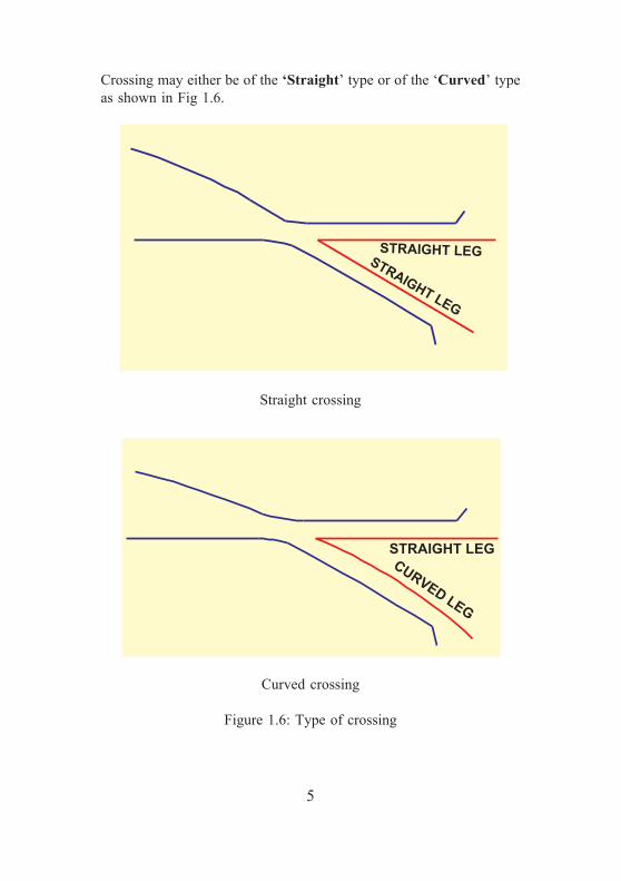
Crossing may either be of the ‘Straight’ type or of the ‘Curved’ typeas shown in Fig 1.6.

Straight crossing

Curved crossing

Figure 1.6: Type of crossing

6

The standard Layouts of various Turnouts in use on Indian Railwaysare shown in Table 1.1

Table 1.1

S.No Crossing Types of SwitchesAngle B.G. M.G.

1. 1 in 8.5 Straight Curved Straight Curved2. 1 in 12 Straight Curved - Partly Curved3. 1 in 16 - Curved - Curved4. 1 in 20 - Curved - -5. 1 in 24* - Curved - -

* Under Standardisation

In the latter case, one of the legs of the crossing is curved to the sameradius as the lead curve, or in other words, the lead curve continuesthrough the crossing. This naturally results in a flatter lead curve thanin the case of a straight crossing for a given crossing angle. However,on Indian Railways only straight crossings are in use. Crossing can beof two types on the basis of material i.e. either Built Up (BU) or CastManganese Steel Crossing (CMS) crossing.

Lead curve has to be tangential to the switch at its heel and to the cross-ing at its toe so as to avoid kinks in the geometry. Subject to these twoconstraints, the lead curve may take one of the following forms;

• Simple Circular Curve• Partly Curved, having a straight length near the crossing• Transition Curve

By combining different types of switches and crossings with differentforms of lead curves, a large variety of geometrical layouts can be ob-tained, each with its own characteristics of lead length and lead radius.The standard practice in India has so far been to use one particularswitch with a particular crossing.

7

1.0 (b) - Provisions of Indian Railway Permanent Way Manual(IRPWM)

Layout Calculations should be performed keeping in view the relevantprovisions as contained in para 410 (2) & 410 (3) and 412 of IRPWM.The same has been reproduced for ready reference.

Para 410(2) of IRPWM

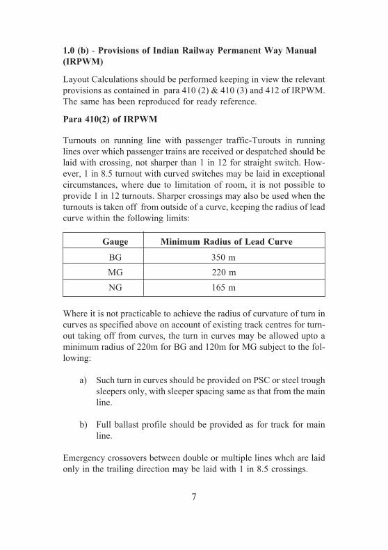
Turnouts on running line with passenger traffic-Turouts in runninglines over which passenger trains are received or despatched should belaid with crossing, not sharper than 1 in 12 for straight switch. How-ever, 1 in 8.5 turnout with curved switches may be laid in exceptionalcircumstances, where due to limitation of room, it is not possible toprovide 1 in 12 turnouts. Sharper crossings may also be used when theturnouts is taken off from outside of a curve, keeping the radius of leadcurve within the following limits:

Gauge Minimum Radius of Lead Curve

BG 350 mMG 220 mNG 165 m

Where it is not practicable to achieve the radius of curvature of turn incurves as specified above on account of existing track centres for turn-out taking off from curves, the turn in curves may be allowed upto aminimum radius of 220m for BG and 120m for MG subject to the fol-lowing:

a) Such turn in curves should be provided on PSC or steel troughsleepers only, with sleeper spacing same as that from the mainline.

b) Full ballast profile should be provided as for track for mainline.

Emergency crossovers between double or multiple lines whch are laidonly in the trailing direction may be laid with 1 in 8.5 crossings.

8

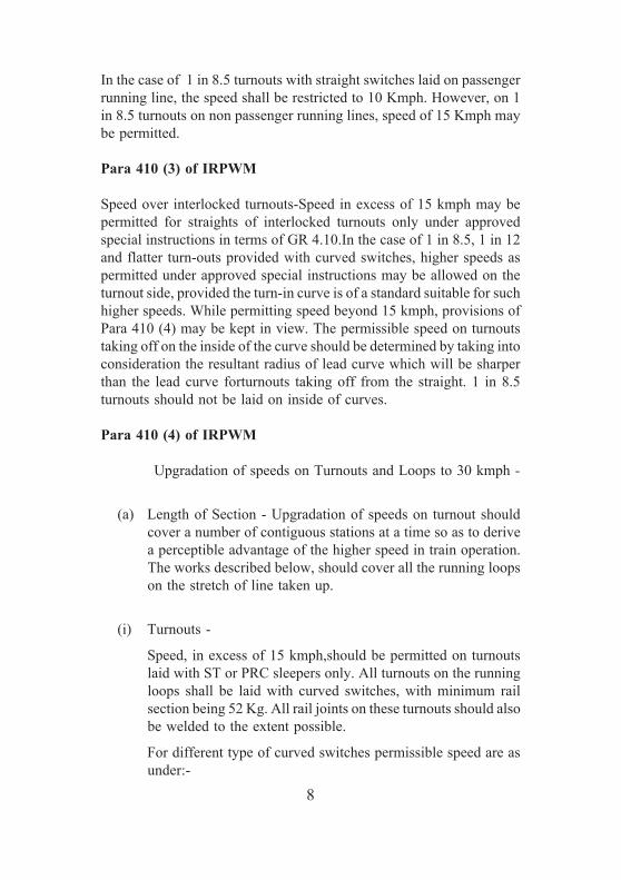
In the case of 1 in 8.5 turnouts with straight switches laid on passengerrunning line, the speed shall be restricted to 10 Kmph. However, on 1in 8.5 turnouts on non passenger running lines, speed of 15 Kmph maybe permitted.

Para 410 (3) of IRPWM

Speed over interlocked turnouts-Speed in excess of 15 kmph may bepermitted for straights of interlocked turnouts only under approvedspecial instructions in terms of GR 4.10.In the case of 1 in 8.5, 1 in 12and flatter turn-outs provided with curved switches, higher speeds aspermitted under approved special instructions may be allowed on theturnout side, provided the turn-in curve is of a standard suitable for suchhigher speeds. While permitting speed beyond 15 kmph, provisions ofPara 410 (4) may be kept in view. The permissible speed on turnoutstaking off on the inside of the curve should be determined by taking intoconsideration the resultant radius of lead curve which will be sharperthan the lead curve forturnouts taking off from the straight. 1 in 8.5turnouts should not be laid on inside of curves.

Para 410 (4) of IRPWM

Upgradation of speeds on Turnouts and Loops to 30 kmph -

(a) Length of Section - Upgradation of speeds on turnout shouldcover a number of contiguous stations at a time so as to derivea perceptible advantage of the higher speed in train operation.The works described below, should cover all the running loopson the stretch of line taken up.

(i) Turnouts -

Speed, in excess of 15 kmph,should be permitted on turnoutslaid with ST or PRC sleepers only. All turnouts on the runningloops shall be laid with curved switches, with minimum railsection being 52 Kg. All rail joints on these turnouts should alsobe welded to the extent possible.

For different type of curved switches permissible speed are asunder:-

9

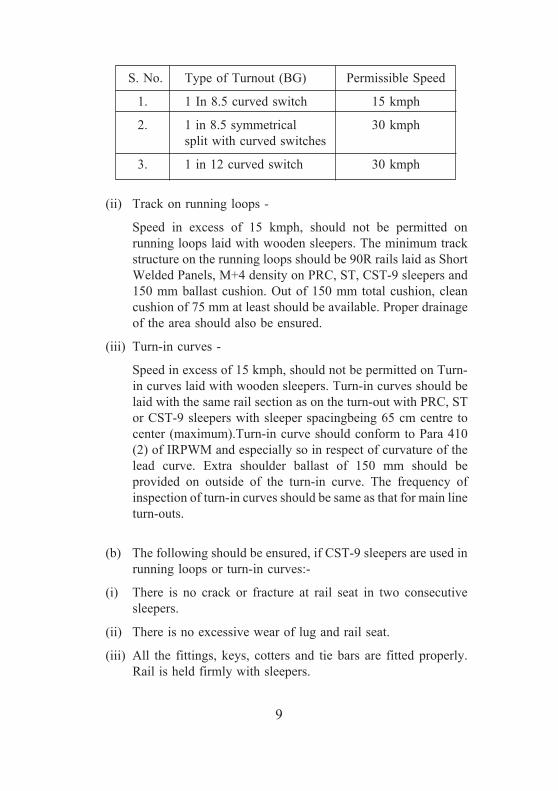
S. No. Type of Turnout (BG) Permissible Speed

1. 1 In 8.5 curved switch 15 kmph

2. 1 in 8.5 symmetrical 30 kmphsplit with curved switches

3. 1 in 12 curved switch 30 kmph

(ii) Track on running loops -

Speed in excess of 15 kmph, should not be permitted onrunning loops laid with wooden sleepers. The minimum trackstructure on the running loops should be 90R rails laid as ShortWelded Panels, M+4 density on PRC, ST, CST-9 sleepers and150 mm ballast cushion. Out of 150 mm total cushion, cleancushion of 75 mm at least should be available. Proper drainageof the area should also be ensured.

(iii) Turn-in curves -

Speed in excess of 15 kmph, should not be permitted on Turn-in curves laid with wooden sleepers. Turn-in curves should belaid with the same rail section as on the turn-out with PRC, STor CST-9 sleepers with sleeper spacingbeing 65 cm centre tocenter (maximum).Turn-in curve should conform to Para 410(2) of IRPWM and especially so in respect of curvature of thelead curve. Extra shoulder ballast of 150 mm should beprovided on outside of the turn-in curve. The frequency ofinspection of turn-in curves should be same as that for main lineturn-outs.

(b) The following should be ensured, if CST-9 sleepers are used inrunning loops or turn-in curves:-

(i) There is no crack or fracture at rail seat in two consecutivesleepers.

(ii) There is no excessive wear of lug and rail seat.

(iii) All the fittings, keys, cotters and tie bars are fitted properly.Rail is held firmly with sleepers.

10

(iv) Tie bars should not be broken or damaged by falling brake gear,wagon parts etc. and they should not have excessive corrosionor elongated holes. The corrosion of tie-bars inside the CST-9plate should be especially checked as this results in theirremoval and adjustment becoming difficult.

(c) The following should be ensured, if ST sleepers are used inTurnouts, Turn-in curves or running loops:-

(i) There is no crack or fracture at rail seat in two consecutivesleepers.

(ii) There is no excessive wear of lug, MLJ and rail seat.

(iii) All the fittings are effective and rail is held with sleepersproperly.

(iv) The sleepers and fittings do not have excessive corrosion,elongated holes etc

Para 412 of IRPWM

No change of superelevation over turn-outs–

There should be no change of cant between points 20 metres on B. G.15meters on M.G., and 12 metres on N. G. outside the toe of the switchand the nose of the crossing respectively, except in cases where pointsand crossings have to be taken off from the transitioned portion of acurve.

Normally, turn-outs should not be taken off the transitioned portion ofa main line curve. However, in exceptional cases, when such a courseis Unavoidable a specific relaxation may be given by the ChiefEngineer of the Railway. In such cases change of cant and/or curvaturemay be permitted at the rates specified in para 407 of IRPWM or suchlesser rates as may be prescribed.

1.0 (c) - Provisions of schedule of dimension 2004 (Revised)Points and crossings:Maximum clearance of check railopposite nose of crossing 48mm

11

Note :

(a) In case of turnouts laid with 1673mm gauge, the clearanceshall be 45mm instead of 48mm

(b) In the obtuse crossing of diamond crossings, the clearances atthe throat of the obtuse crossing shall be 41mm

Minimum clearance of check railopposite nose of crossing 44mm

Note :

(a) In case of turnouts laid with 1673mm gauge, the clearanceshall be 41mm instead of 44mm

(b) In the obtuse crossing of diamond crossings the clearance atthe throat of the obtuse crossing shall be 41mm

Maximum clearance of wing rail at nose of crossing 48mm

Note :In case of turnouts laid with 1673mm gauge, the clearance shall be41mm instead of 44mm.

Minimum clearance of wing rail at nose of crossing 44mm

Note :In case of turn outs laid with 1673mm gauge, the clearance shall be41mm instead of 44mm.

Minimum clearance between toe of open switch and stock rail

(i) For existing works 95mm

(ii) For new works or alteration to existing works 15mm

Note :

The clearance can be increased upto 160mm in curved switchesin order to obtain adequate clearance between gauge face ofstock rail and back face of tongue rail.

12

Minimum radius of curvature for slip points, turnouts of crossoverroads 218 metres (8 degree)

Note :In special cases mentioned below this may be reduced to not less thanthe minimum of

(i) 213m radius in case of 1 in 8.5 BG turnouts with 6.4m overriding switch, and

(ii) 175m radius in case of 1 in 8.5 scissors crossing to allow forsufficient straight over the diamond crossing betweencrossovers.

Minimum angles of crossing (ordinary) 1 in 16

Note :

Crossings as flat as 1 in 20 will usually be sanctioned ifrecommended by the Commissioner of Railway Safety.

Diamond crossings not to be flatter than 1 in 8.5

Note :Diamond Crossings as flat as 1 in 10 will usually be sanctioned ifrecommended by the Commissioner of Railway Safety.

Minimum length of tongue rail 660mm

Minimum length of train protection, point locking or fouling treadle bar12800mm

Note :There must be no change of superelevation (of outer over inner rail)between points 18m outside toe of switch rail and nose of crossingrespectively, except in the case of special crossings leading to snagdead-ends or under circumstances as provided for in item-22.

Super elevation and speed in stations on curves with turnouts ofcontrary and similar flexure:

13

Main line: Subject to the permissible run through speed, based on thestandard of. Interlocking, the equilibrium superelevation, calculated forthe speed of the fastest train, may be reduced by a maximum amount of75mm without reducing the speed on the mainline.

1.1 Layout Calculations

A yard may require various combinations of turnouts (i.e. switches,leads & crossings), with curves and straights, to transfer trains from onetrack to another or enable trains to cross other tracks. Depending uponthe requirements, these combinations are known as layouts. Forsatisfying the various geometrical features of the layouts, one has toperform variety of trigonometric calculations and hence the name‘Layout Calculations’.

Understanding of Layout Calculations is necessary for fixing thecorrect position of turnouts with respect to the existing tracks in case ofremodelling of an yard or for designing an altogether new layouts.Turnouts can be fixed either by locating Stock Rail Joint(SRJ) or bylocating Theoretical Nose of Crossing (TNC). SRJ/TNC can be locatedby ‘Centre Line, ‘Outer Rail’ or ‘Graphical’ method .

In ‘Centre Line’ method, the turnout is represented by center lines ofstraight and turnout side. This method is primarily used for locating SRJfor the cases when turnouts are taking off from Straight tracks.

In ‘Outer Rail’ method, the turnout is represented fully by drawing theleft rail and right rail of the turnout. This method is primarily used forlocating TNC for the cases when turnouts are taking off from the curvedtracks. However, this method is more versatile but cumbersome and canalso be used for the cases when turnouts are taking off from straighttracks.

In ‘Graphical’ method, the entire drawing will be made on computerby use of relevant drafting software like AutoCAD. After replicatingthe layout on the computer, all the calculations can be performedgraphically. Now a days various advanced softwares are available.MX-Rail is one of the specialized software developed for the railwayindustry. Yard calculations are one of the powerful feature of thissoftware

14

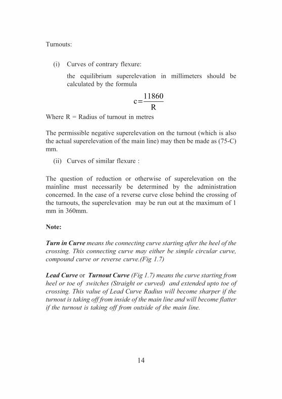
Turnouts:

(i) Curves of contrary flexure:

the equilibrium superelevation in millimeters should becalculated by the formula

R11860c=

Where R = Radius of turnout in metres

The permissible negative superelevation on the turnout (which is alsothe actual superelevation of the main line) may then be made as (75-C)mm.

(ii) Curves of similar flexure :

The question of reduction or otherwise of superelevation on themainline must necessarily be determined by the administrationconcerned. In the case of a reverse curve close behind the crossing ofthe turnouts, the superelevation may be run out at the maximum of 1mm in 360mm.

Note:

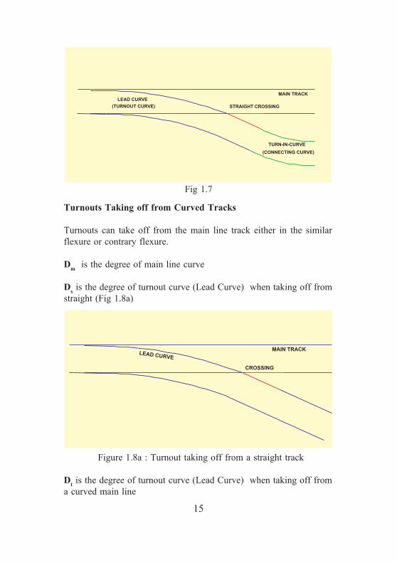
Turn in Curve means the connecting curve starting after the heel of thecrossing. This connecting curve may either be simple circular curve,compound curve or reverse curve.(Fig 1.7)

Lead Curve or Turnout Curve (Fig 1.7) means the curve starting fromheel or toe of switches (Straight or curved) and extended upto toe ofcrossing. This value of Lead Curve Radius will become sharper if theturnout is taking off from inside of the main line and will become flatterif the turnout is taking off from outside of the main line.

15

Turnouts Taking off from Curved Tracks

Turnouts can take off from the main line track either in the similarflexure or contrary flexure.

Dm is the degree of main line curve

Ds is the degree of turnout curve (Lead Curve) when taking off fromstraight (Fig 1.8a)

Figure 1.8a : Turnout taking off from a straight track

Dt is the degree of turnout curve (Lead Curve) when taking off froma curved main line

Fig 1.7

16

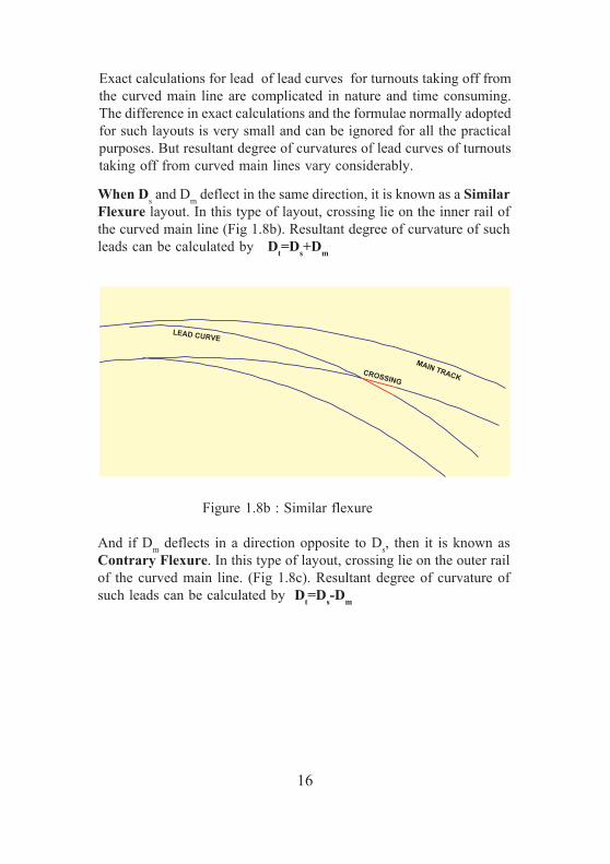
Exact calculations for lead of lead curves for turnouts taking off fromthe curved main line are complicated in nature and time consuming.The difference in exact calculations and the formulae normally adoptedfor such layouts is very small and can be ignored for all the practicalpurposes. But resultant degree of curvatures of lead curves of turnoutstaking off from curved main lines vary considerably.

When Ds and Dm deflect in the same direction, it is known as a SimilarFlexure layout. In this type of layout, crossing lie on the inner rail ofthe curved main line (Fig 1.8b). Resultant degree of curvature of suchleads can be calculated by Dt=Ds+Dm

Figure 1.8b : Similar flexure

And if Dm deflects in a direction opposite to Ds, then it is known asContrary Flexure. In this type of layout, crossing lie on the outer railof the curved main line. (Fig 1.8c). Resultant degree of curvature ofsuch leads can be calculated by Dt=Ds-Dm

17

Figure 1.8c : Contrary flexure

When Dt and Dm are equal in a contrary flexure, then it is known asSymmetrical Split. (Fig 1.8d)

Figure 1.8d : Symmetrical split

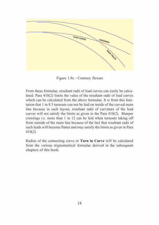
Sometimes it may so happen that crossing lie on the outer rail of thecurved main line and even then deflecting in the same direction as thatin the similar flexure.(Fig 1.8e) Resultant degree of curvature of suchleads can be calculated by Dt=Dm-Ds

18

Figure 1.8e : Contrary flexure

From these formulae, resultant radii of lead curves can easily be calcu-lated. Para 410(2) limits the value of the resultant radii of lead curveswhich can be calculated from the above formulae. It is from this limi-tation that 1 in 8.5 turnouts can not be laid on inside of the curved mainline because in such layout, resultant radii of curvature of the leadcurves will not satisfy the limits as given in the Para 410(2). Sharpercrossings i.e. more than 1 in 12 can be laid when turnouts taking offfrom outside of the main line because of the fact that resultant radii ofsuch leads will become flatter and may satisfy the limits as given in Para410(2)

Radius of the connecting curve or Turn in Curve will be calculatedfrom the various trignometrical formulae derived in the subsequentchapters of this book.

19

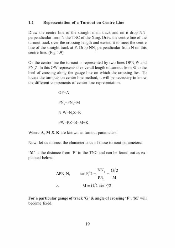
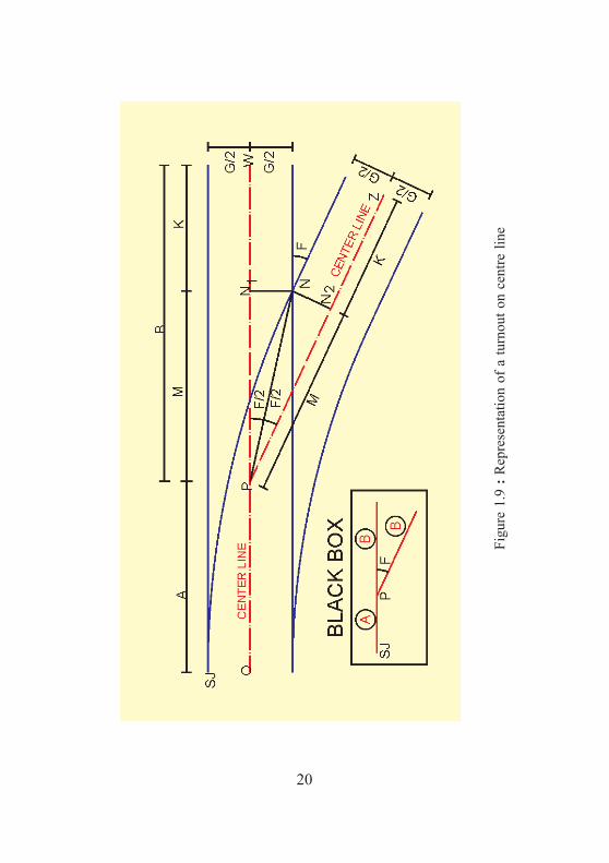
1.2 Representation of a Turnout on Centre Line

Draw the centre line of the straight main track and on it drop NN1perpendicular from N the TNC of the Xing. Draw the centre line of theturnout track over the crossing length and extend it to meet the centreline of the straight track at P. Drop NN2 perpendicular from N on thiscentre line. (Fig 1.9)

On the centre line the turnout is represented by two lines OPN1W andPN2Z. In this OW represents the overall length of turnout from SJ to theheel of crossing along the gauge line on which the crossing lies. Tolocate the turnouts on centre line method, it will be necessary to knowthe different components of centre line representation.

OP=A

PN1=PN2=M

N1W=N2Z=K

PW=PZ=B=M+K

Where A, M & K are known as turnout parameters.

Now, let us discuss the characteristics of these turnout parameters:

‘M’ is the distance from ‘P’ to the TNC and can be found out as ex-plained below:

11

1

NN G 2ΔPN N, tan F 2

PN M

M G 2 cot F 2

= =

∴ =

For a particular gauge of track ‘G’ & angle of crossing ‘F’, ‘M’ willbecome fixed.

20

Figu

re 1

.9 :

Rep

rese

ntat

ion

of a

turn

out o

n ce

ntre

line

21

‘K’ is the length of the back leg of crossing and will be dependent upontype of crossing i.e. BU or CMS crossing. Therefore for a particulartype of crossing chosen for a yard, value of ‘K’ will be fixed.Likewise, B=M+K will also become fixed.

‘A’ is the distance between ‘SJ’ to ‘Point of intersection ‘P’ of centerline of mainline and turnout side which is basically dependent uponangle of crossing and not on type of switches or else whole yard willhave to be redesigned in case of adopting new design of switches. Asdiscussed earlier that value of ‘M’ is fixed for a particular gauge oftrack & angle of crossing and hence distance between SJ to P i.e ‘A’will also be fixed.

In view of the above, it is therefore obvious that for a given gauge,crossing angle and crossing type (BU or CMS), value of these turnoutparameters i.e. ‘A’, ‘M’ & ‘K’ are fixed. This can be convenientlyunderstood as a Black Box (see Fig 1.9) containing a geometrical figurethe dimensions of which are fixed. Then the rest is to fix this Black Boxwith respect to the existing yard geometry so as to satisfy all thegeometrical conditions of the yard.

22

Chapter 2

Lead and Radius of IRS Turnout

2.1 (a) IRS Turnout with Straight SwitchesCalculation of length of lead curve and radius of leadcurve

The lead curve in IRS turnout with straight switches are placedtangential to the tongue rail at the heel and to the front straight leg ofthe crossing. (Fig 2.1)

Figure 2.1: IRS Turnout with straight switches

23

Formulae

( )

( )

( )

In BMK; BM MK (Each being tangent length)F-β

MBK MKB2

F βF-βIn Δ BKC; BKC F-22

BC AD AB CD AD AB KP G d wSinFF β F β

KC BCCot G d wSinF Cot2 2

Lead DE DP PE KC PE F β

Lead G d wSinF Cot wCosF (22

Δ =

∠ = ∠ =

+∠ = =

= − − = − − = − −+ +

= = − −

= = + = ++

= − − + .1)

In ΔOBK; BOK F-β, OB OK RF-β F-β

BK RSin 2RSin 2 2

F-β BK 2RSin (2.1a)

2BC G d wSinF

also in ΔBKC; BK (2.1b)F β F βSin Sin2 2

F-β G d wSinFequating Eq 2.1a & 2.1 b; 2RSin F β2 Sin

2G d

Radius R

+

∠ = = =

=

∴ =

− −= =+ +

− −= +

− −∴ = =

wSinF(2.2)F β F β2Sin Sin

2 2 R radius of lead curve, d heel divergence

w straight leg of crossing ahead of TNC, β switch angle

G =Track gauge

Where

+ −

= =

= =

24

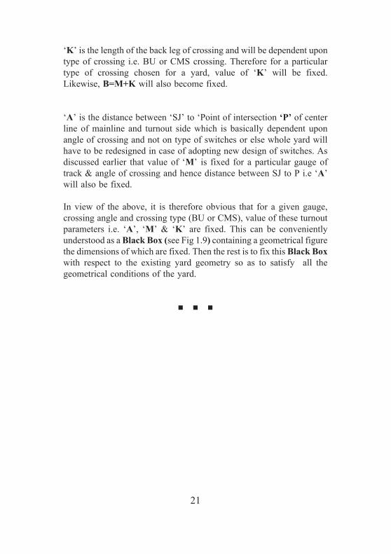
2.1 (b) IRS Turnout with straight switchCalculation of offsets to lead curves

The lead curve is extended from heel at point ‘B’ to a point ‘H’ so thatthe tangent to the curve runs parallel to the gauge line at a distance ‘Y’(offset) as shown in Fig 2.2.

Figure 2.2: Offsets to lead curves for IRS turnout withstraight switches

25

The point ‘H’ has been shown to lie inside the track, but in certainlayouts, depending on the switch angle and the radius, the point ‘H’may lie outside the track and therefore the value of ‘Y’ will work outas negative. The distance ‘BQ’ be denoted by ‘L’.

0

In KOJ,

OK R, KOJ F, OJK 90

JK OKSinF RSinFF β

CK (G-d-wSinF)Cot2

CJ BQ L JK CKF β

CJ RSinF (G-d-wSinF)Cot (2.3)2

OI OH HI R Y (2.4)

also, OI OJ JI RCosF G-wSinF (2.5)

equating (2

Δ

= ∠ = ∠ =

= =+

=

= = = −+

∴ = −

= + = +

= + = +

( )

( )

.4) & (2.5),

R Y RCosF G-wSinF

Y G-wSinF-R 1-CosF (2.6)

: It is also possible to work out values of 'L' & 'Y'

directly from OBQ,

BQ = L RSinβ (2.7)

Y d-R 1-Cosβ (2.8)

But a word of cautio

Note

+ = +

∴ =

Δ

=

=

n is that as the value of 'β' is very small, it is

difficult to get the correct values of Cosβ as variations in the region

are not uniform. 'L' , however can be derived from L RSinβ=

26

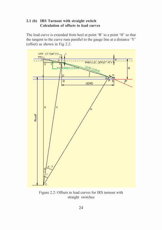
Example 2.1

Calculate the lead and the radius of a 1 in 8.5 IRS turnout with straightswitches.

Given: G=1676mm, d=136mm, w=864mm

( )

( )

F βLead G d wSinF Cot wCosF

20 ' " 0 ' "6 42 35 1 34 270 ' " 1676 136 864 Sin6 42 35 Cot

20 ' " 864 Cos6 42 35

19871.79 858.08 20729.87mm 20730mmG d wSinF

R F β F β2Sin Sin2 2

0 ' "1676 136 864 Sin6 42 350 ' "6 42 352 Sin

+= − − +

+= − − ×

+ ×

= + = ≈− −

= + −

− − ×=

+×0 ' " 0 ' " 0 ' "1 34 27 6 42 35 1 34 27Sin

2 2222358.34mm 222358mm & ay 222.36 m

−

= ≈

0 ' " 0 ' "F 6 42 35 , β 1 34 27= =

2.2 IRS Turnout with Curved Switches - Calculation of lengthof lead curve and radius of lead curve

The lead curves in these layouts at toe of switches are tangential to theswitch angle and meets the straight leg of crossing at a distance ‘w’from the TNC of the crossing. (Fig 2.2)

27

Figure 2.3: IRS Turnout with curved switches

28

At toe of switch, thickness of tongue rail is ‘t’. Derivation for lead curveradius will be same as for IRS straight switches. The same can bederived by substituting ‘t’ (toe thickness) for ‘d’ (the heel divergence).

Formulae

For fixing positions of heel, it is necessary to find the point whereoffset to the lead curve from main line will be equal to heeldivergence ‘d’. For this, same principles are applied as for findingoffsets to lead curve for straight IRS turnouts. It is, however,cautioned that the new tangent is drawn after extending the curve, soas to lie parallel to the main line, may be outside the track anddistance ‘Y’ may come out as negative or positive. It has to be appliedwith its positive or negative sign arithmetically.

F βL BQ CJ KJ-CK RSinF-(G-t-wSinF)Cot 2+= = = = (2.11)

, from OQB, or Δ

L BQ RSinβ = = (2.12)

( )Y G-wSinF-R 1-CosF= (2.13)

2Switch Length, SL 2R(d-Y)-(d-Y) L= − (2.14)

F βLead (G-t-wSinF)Cot SL wCosF2+= − + (2.15)

F βCK (G-t-wSinF)Cot (2.9)

2G-t-wSinF

Radius of Lead Curve, R (2.10)F β F β2Sin Sin2 2

+=

= + −

29

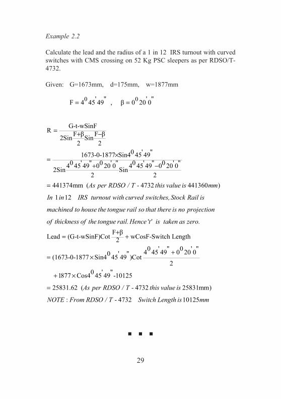
Example 2.2

Calculate the lead and the radius of a 1 in 12 IRS turnout with curvedswitches with CMS crossing on 52 Kg PSC sleepers as per RDSO/T-4732.

Given: G=1673mm, d=175mm, w=1877mm

G-t-wSinFR F β F β2Sin Sin

2 20 ' "1673-0-1877 Sin4 45 49

0 ' " 0 ' " 0 ' " 0 ' "4 45 49 0 20 0 4 45 49 0 20 02Sin Sin2 2

441374mm ( 4732 441360 )

1 12

As per RDSO / T - this value is mm

In in IRS turnout with curved switches, Stock

= + −

×=

+ −

=

F βLead (G-t-wSinF)Cot wCosF-Switch Length 2

0(1673-0-1877 Sin4 4

Rail is

machined to house the tongue rail so that there is no projection

of thickness of the tongue rail. Hence 't' is taken as zero.+= +

= ×0 ' " 0 ' "4 45 49 0 20 0' "5 49 )Cot

20 ' " 1877 Cos4 45 49 -10125

25831.62 ( 4732 25831mm)

: 4732 10125

As per RDSO / T - this value is

NOTE From RDSO / T - Switch Length is mm

+

+ ×

=

0 0' " ' "F 4 45 49 , β 0 20 0= =

30

Chapter 3

Connections to Diverging Tracks

3.1 Connections to Diverging Tracks

Connection to non parallel sidings from an existing line can be of threetypes depending upon the comparative values of ‘θ’ and ‘F’. Where ‘θ’is the angle of intersection between the two lines and ‘F’ is the angleof crossing used for connection. There may be three situations viz;

Now because of the local obstructions on the existing line, there can befurther two sub categories namely; i.e Without obligatory points andWith obligatory points on the main line. Therefore, connections todiverging tracks may have following situations;

For θθθθθ = F

Case I Without obligatory point on main lineCase II With obligatory point on the main line

For θθθθθ > F

Case III Without obligatory point on main lineCase IV With obligatory point on the main line

For θθθθθ < F

Case V Without obligatory point on main lineCase VI With obligatory point on the main line

θ F

θ F

and θ F

=

>

<

31

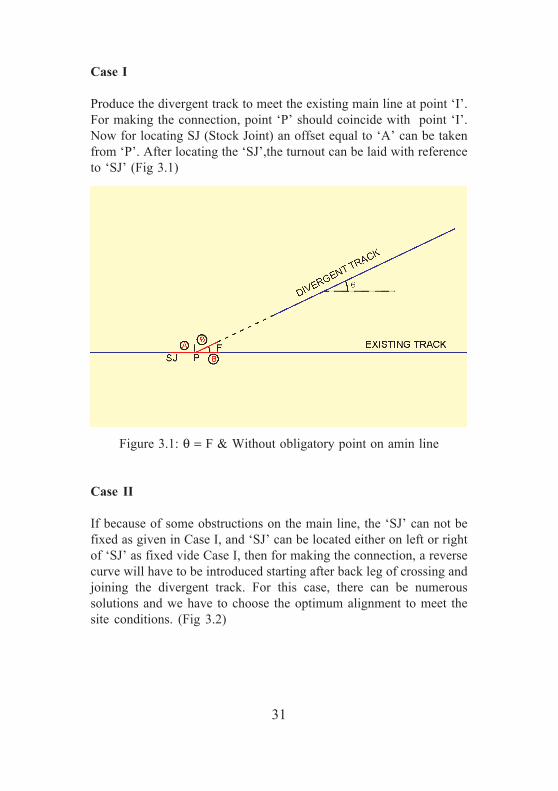
Case I

Produce the divergent track to meet the existing main line at point ‘I’.For making the connection, point ‘P’ should coincide with point ‘I’.Now for locating SJ (Stock Joint) an offset equal to ‘A’ can be takenfrom ‘P’. After locating the ‘SJ’,the turnout can be laid with referenceto ‘SJ’ (Fig 3.1)

Figure 3.1: θ = F & Without obligatory point on amin line

Case II

If because of some obstructions on the main line, the ‘SJ’ can not befixed as given in Case I, and ‘SJ’ can be located either on left or rightof ‘SJ’ as fixed vide Case I, then for making the connection, a reversecurve will have to be introduced starting after back leg of crossing andjoining the divergent track. For this case, there can be numeroussolutions and we have to choose the optimum alignment to meet thesite conditions. (Fig 3.2)

32

Figure 3.2: θ = F & With obligatory point on main line

Case III

In this case, if we are having the liberty in fixing the ‘SJ’, it should beon the left hand side of point of intersection ‘I’. ( Fig 3.3)

Figure 3.3: θ > F & Without obligatory point on main line

33

Formulae

(3.4)TSinθT)SinF(BY

(3.3)AXOL

(3.2)TCosθT)CosF(BX

(3.1)2

FθRtanT

++=

+=

++=

−=

Interpretation of Formulae & Field Practicalities

Intersection angle ‘θ’ has to be found out from the field surveying. Theradius ‘R’ of the connecting curve has to be assumed. Normally thevalue of connecting curve radius is taken equal to that of radius of turnoutcurve. Now value of ‘T’ can be calculated from Eq:3.1. Once ‘T’ isknown, the value of ‘X’ & ‘Y’ can be calculated fron Eq:3.2 & 3.4respectively. Having thus calculated the value of ‘X’ & ‘Y’, ‘TP2’ islocated first as the intersection point between the divergent track and aline drawn parallel to the existing track at a distance ‘Y’ and the locationof ‘SJ’ is marked with reference to TP2 by drawing a perpendicular offsetat a distance ‘OL’ from ‘TP2.’ (Fig 3.3a)

Figure 3.3a

34

Now after locating ‘SJ’, the turnout is linked and then the connectingcurve is provided with radius equal to ‘R’. This connecting curve willbe starting from back of crossing (TP1) and ending at ‘TP2’, thusestablishing the full connection.

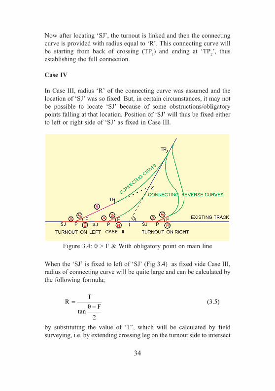
Case IV

In Case III, radius ‘R’ of the connecting curve was assumed and thelocation of ‘SJ’ was so fixed. But, in certain circumstances, it may notbe possible to locate ‘SJ’ because of some obstructions/obligatorypoints falling at that location. Position of ‘SJ’ will thus be fixed eitherto left or right side of ‘SJ’ as fixed in Case III.

Figure 3.4: θ > F & With obligatory point on main line

When the ‘SJ’ is fixed to left of ‘SJ’ (Fig 3.4) as fixed vide Case III,radius of connecting curve will be quite large and can be calculated bythe following formula;

by substituting the value of ‘T’, which will be calculated by fieldsurveying, i.e. by extending crossing leg on the turnout side to intersect

TR (3.5)

θ Ftan

2

=−

35

divergent track at ‘Z’. Thus TP1Z will be the tangent length ‘T’. Nowthe connecting curve of radius ‘R’ can be laid at the site. In this case,the radius ‘R’ of the connecting curve will be large, which can bereduced by providing a straight after the heel of crossing andconnecting curve starting after this straight. For this case formulae canbe modified as follows;

Figure 3.5: θ < F & Without obligatory point on main line

Now in another situation, when ‘SJ’ is located on right of ‘SJ’ (Fig 3.4)as fixed vide case III, there can be numerous solutions and an optimumalignment can be decided keeping in view the site conditions. In thiscase, connecting curve will have to be a reverse curve.

Case V

In this case, if we are having the liberty in fixing the ‘SJ’, it should beon the right hand side of point of intersection ‘I’. (Fig 3.5)

θ-FT Rtan (3.6)

2X (B S T)CosF TCosθ (3.7)

OL X A (3.8)

Y (B S T)SinF TSinθ (3.9)

=

= + + +

= +

= + + +

36

Formulae

(3..13)TSinθT)SinF(BY

(3.12)AXOL

(3.11)TCosθT)CosF(BX

(3.10) 2

θ-FRtanT

++=

+=

++=

=

Interpretation of Formulae & Field Practicalities

Intersection angle‘θ’ has to be found out from the field surveying. Theradius ‘R’ of the connecting curve has to be assumed. Normally thevalue of radius ‘R’ is taken equal to that of the radius of turnout radius.Now value of ‘T’ is calculated from Eq 3.9. Once ‘T’ is known, thevalue of ‘X’, ‘OL’ & ‘Y’ can be calculated from Eq 3.11, 3.12 & 3.13respectively. ‘TP2’ is located first as the intersection point between thedivergent track and a line drawn parallel to the existing track at adistance ‘Y’ and the location of ‘SJ’ is marked with reference to ‘TP2’by drawing a perpendicular offset at a distance ‘OL’ from ‘TP2’(Fig 3.5a)

Figure 3.5a

θ

37

Now after locating ‘SJ’, the turnout is linked and then the connectingcurve is provided with a radius equal to ‘R’. Thus connecting curve willbe starting from back of crossing (TP1) and ending at ‘TP2’, thusestablishing the full connection.

Case VI

In case V, radius of ‘R’ of the connecting curve was assumed and thelocation of ‘SJ’ was to be fixed. But in certain circumstances, it may notbe possible to fix ‘SJ’ because of some obstructions/obligatory pointsfalling at that location. Position of ‘SJ’ will thus be fixed either to theleft or right side of ‘SJ’ as fixed in Case IV. ( Fig 3.6)

When the ‘SJ’ is to be located on right of ‘SJ’ as fixed vide Case V,radius ‘R’ of connecting curve will be quite large and can be calculatedby the following formulae;

Figure 3.6: θ < F & With obligatory point on main line

TR (3.14)

F-θtan

2

=

38

Now, in another situation, when ‘SJ’ is located on right of ‘SJ’ as fixedvide Case V, there can be numerous solutions and an optimumalignment can be decided keeping in view the site conditions. In thiscase, connecting curve has to be a reverse curve.

F-θT Rtan (3.15)

2X (B S T)CosF TCosθ (3.16)

OL X A (3.17)

Y (B S T)SinF TSinθ (3.18)

=

= + + +

= +

= + + +

by substituting the value of ‘T’, which will be calculated by fieldsurveying, i.e by extending crossing leg of the turnout side to intersectdivergent track at ‘Z’. TP1 will be the tangent length ‘T’. Now theconnecting curve of radius ‘R’ can be laid at the site. In this case, radius‘R’ of the connecting curve will be large, which can be reduced byproviding a straight after the heel of crossing and connecting curvestarting after this straight. For this case formulae can be modified asfollows:

39

Example 3.1

A broad gauge siding is required to be connected to a main line trackusing a 52 Kg, 1 in 12 T/O. The angle of intersection between the twotracks being 100. Calculate the required distances for the layoutassuming that the connecting curve starts from the heel of crossing.

Given: F=4045’49”, A=16.953m, B=23.981m, R=441.282m

0 0

0 0

θ FT Rtan

2' "10 -4 45 49

441.282tan2

20.179m

X (B T)CosF TCosθ' " (23.981 20.179)Cos4 45 49 (20.179)Cos10

44.007 19.872

63.879m

OL X A 63.879 16.953 80.832m

Y (B T)SinF TSinθ

−=

=

=

= + +

= + +

= +

=

= + = + =

= + +0 0' " (23.981 20.179)Sin4 45 49 (20.179)Sin10

3.667 3.504

7.171m

= + +

= +

=

40

Example 3.2

A broad gauge siding is required to be connected to a main line trackusing 52 kg (PSC) (CMS) , 1 in 8.5 T/O. The angle of intersectionbetween the two tracks is 30. Calculate the required distances for thelayout.

Given: F = 6042’35”, A=12.025m, B=16.486m, R = 221.522m

F-θT Rtan

20 ' " 06 42 35 3

221.522tan2

7.174m

X (B T)CosF TCosθ0 ' " 0 (16.486 7.174)Cos6 42 35 (7.174)Cos3

23.495 7.164 30.659

X 30.659m

OL X A 30.659 12.025 42.684m

Y (B T)SinF TSinθ

=

−=

=

= + +

= + +

= + =

=

= + = + =

= + +0 ' " 0 (16.486 7.174)Sin6 42 35 (7.174)Sin3

2.764 0.375

3.139m

= + +

= +

=

41

Chapter 4

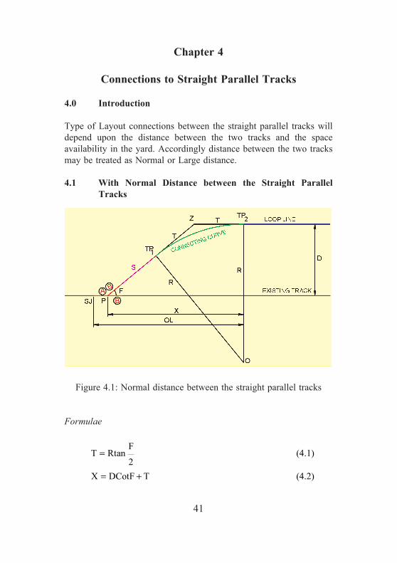
Connections to Straight Parallel Tracks

4.0 Introduction

Type of Layout connections between the straight parallel tracks willdepend upon the distance between the two tracks and the spaceavailability in the yard. Accordingly distance between the two tracksmay be treated as Normal or Large distance.

4.1 With Normal Distance between the Straight ParallelTracks

Figure 4.1: Normal distance between the straight parallel tracks

Formulae

FT Rtan (4.1)

2X DCotF T (4.2)

=

= +

42

Interpretation of Formulae & Field Practicalities

First of all, radius of connecting curve ‘R’ has to be assumed keepingin view the content of Para 410 of IRPWM. Distance between the twostraight parallel track will be found out from the field. Now after havingthe values of ‘R’ and ‘D’, calculate the values of ‘T’, ‘X’, ‘OL’ and ‘S’from Eq 4.1, 4.2, 4.3 and 4.4 respectivly.

Now, in the field, either of the two points i.e. TP2 and ‘SJ’ will bedecided from the site conditions. With respect to one point, the otherpoint will be fixed which will be at a distance ‘OL’ apart. After that,entire layout i.e. turnout, straight after heel of crossing and theconnecting curve can be laid by field surveying.

Note:

In the above connection, it is evident that for a given value of ‘D’, if weincrease/decrease the value of straight ‘S’ after heel of crossing, valueof connecting curve ‘R’ decreases/increases respectively. Therefore, bycontrolling the value of ‘S’, value of ‘R’ can be controlled. For a givenvalue of ‘D’, less the value of ‘S’, more will be the value of ‘OL’ i.e.overall length requirement. More the value of ‘S’, less will be the valueof ‘OL’. For S=0, ‘OL’ will be the maximum. ‘S’ can be increased toa maximum value till the value of ‘R’ reduces to R=R recommended.

Correctness of Layout dependes basically on the correctness of thevalues of different variables as used in the above formulae. Any wrongvalue will disturb the geometry of layout at the field.

OL X A (4.3)

(B S T)SinF D

D S (B T) (4.4)

SinF

= +

+ + =

∴ = − +

43

4.2 Layout Calculations with Fanshaped PSC Layout

Due to introduction of latest versions of 52 Kg and 60 Kg BG(1673 mm), 1 in 16, 1 in 12 and 1 in 8.5 turnouts on PSC sleepers todrawing Nos RDSO/T-5691, RDSO/T-4732, 4218 and RDSO/T-4865respectively. Values of various turnout parameters have been given atthe end of the book in Table of Detailed Dimensions.

Values of these turnout parameters can easily be calculated from therelevant RDSO drawings.

If we take the value of ‘B’ from the table of dimensions for performingthe calculations, we are inadvertently making a mistake and our finallayout will become wrong. The same is explained as detailed below;

The value of ‘B’ as per usual convention for these versions of theturnout is slightly more than for conventional CMS crossing and lessthan that for Built UP crossing. It will be much longer for all practicalpurposes, as the entire layout becomes rigidly straight up to the lastcommon PSC sleeper of the turnout due to prepositioned inserts forstraight alignment behind the heel of crossing.

Due to situation as explained above, it may not be possible to start theconnecting curve just behind the heel of crossing as was done earlier forIRS layouts.

Therefore, by default, the geometry of PSC layouts will be having acertain straight ‘S’ after the heel of crossing which should be accountedfor modifying the value of ‘B’ as given in the Table of DetailedDimensions given at the end of this book. The value of default straightshould be determined from the relevant drawings. Because of theabove, calculations for the various PSC layouts if done as per earliervalues of the turnout parameters is likely to generate kinky alignment,especially for the connecting curve which will tend to become sharperdue to reduction in tangents lengths.

44

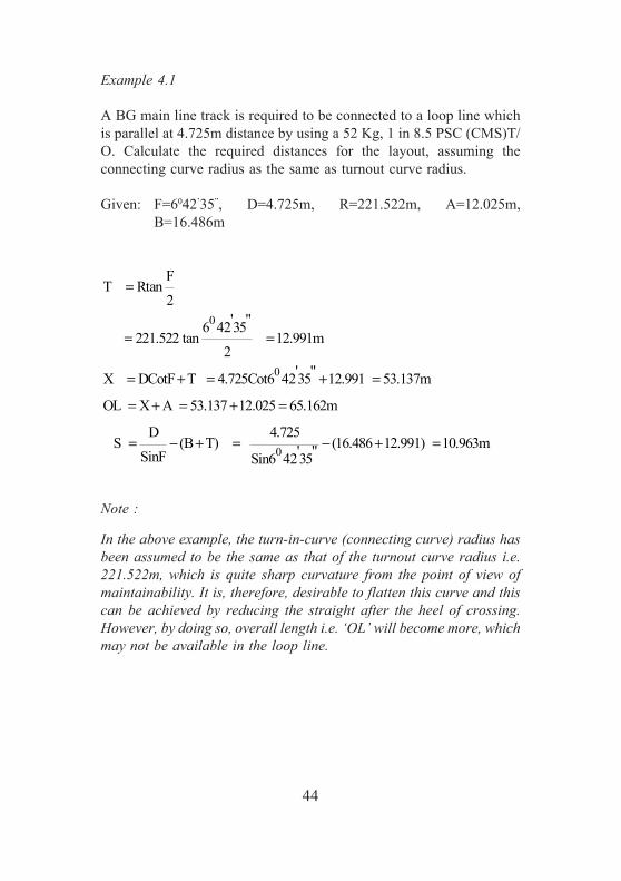
Example 4.1

A BG main line track is required to be connected to a loop line whichis parallel at 4.725m distance by using a 52 Kg, 1 in 8.5 PSC (CMS)T/O. Calculate the required distances for the layout, assuming theconnecting curve radius as the same as turnout curve radius.

Given: F=6042’35”, D=4.725m, R=221.522m, A=12.025m,B=16.486m

Note :

In the above example, the turn-in-curve (connecting curve) radius hasbeen assumed to be the same as that of the turnout curve radius i.e.221.522m, which is quite sharp curvature from the point of view ofmaintainability. It is, therefore, desirable to flatten this curve and thiscan be achieved by reducing the straight after the heel of crossing.However, by doing so, overall length i.e. ‘OL’ will become more, whichmay not be available in the loop line.

0

0

0

FT Rtan

2' "6 4235

221.522 tan 12.991m 2

' "X DCotF T 4.725Cot6 4235 12.991 53.137m

OL X A 53.137 12.025 65.162m

D 4.725 S (B T) (16.486 12.991) 10.963m ' "SinF Sin6 4235

=

= =

= + = + =

= + = + =

= − + = − + =

45

Example 4.2

In the above example 4.1, calculate radius of the flattest turn-in-curveto maintain it satisfactorily. Also calculate the over all length of thelayout.

Given: F=6042’35”, D=4.725m, A=12.025m, B=16.486m

For the flattest turn-in-curve, the straight ‘S’ after the heel of crossingwill be equal to zero.

0

0

DS (B T)

SinFsubstituting S 0,

D(B T)

SinFD 4.725

T B 16.486 23.954m' "SinF Sin6 42 35F

now from equation, T Rtan ,2

T 23.954R 408.629m' "F 6 42 35tan tan2 2X DCotF T

4.725Cot

= − +

=

= +

= − = − =

=

= = =

= +

= 0 ' "6 42 35 23.954 63.817m

OL X A 63.817 12.025 75.842m

which is more by 75.842-65.162 10.068m, in comparison with

overall length requirement as in the previous example 4.1

+ =

= + = + =

=

46

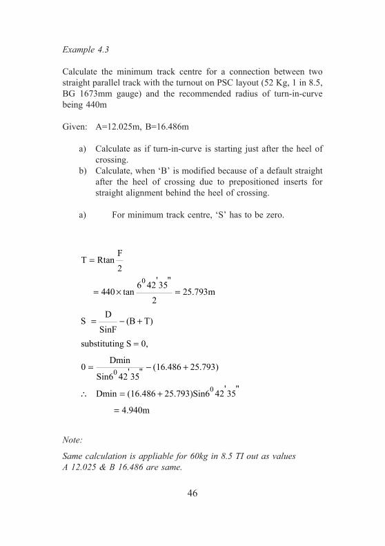
Example 4.3

Calculate the minimum track centre for a connection between twostraight parallel track with the turnout on PSC layout (52 Kg, 1 in 8.5,BG 1673mm gauge) and the recommended radius of turn-in-curvebeing 440m

Given: A=12.025m, B=16.486m

a) Calculate as if turn-in-curve is starting just after the heel ofcrossing.

b) Calculate, when ‘B’ is modified because of a default straightafter the heel of crossing due to prepositioned inserts forstraight alignment behind the heel of crossing.

a) For minimum track centre, ‘S’ has to be zero.

0

0

0

FT Rtan

2' "6 42 35

440 tan 25.793m2

DS (B T)

SinFsubstituting S 0,

Dmin0 (16.486 25.793) ' "Sin6 42 35

' " Dmin (16.486 25.793)Sin6 42 35

4.940m

=

= × =

= − +

=

= − +

∴ = +

=

Note:

Same calculation is appliable for 60kg in 8.5 TI out as valuesA 12.025 & B 16.486 are same.

47

b) The default length of straight, because of prepositionedinserts in PSC layouts after the heel of crossing, should bedetermined from the relevant drawings. For 52 Kg, 1 in8.5 BG 1673mm gauge PSC layout, this straight cansafely be taken as 3.3m.

Therefore, minimum track centre should be say 5.3m to accommodatecompletely the 1 in 8.5 turnout on PSC sleepers, so as to satisfy all thegeometrical conditions.

It is worth mentioning that either because of lesser track centre orwrong calculations, at several yards, last common sleepers are beingremoved so as to start connecting curve slightly earlier. It is thereforerecommended that to accommodate PSC turnouts, the minimum trackcentre must be equal to 5.3m, otherwise either common sleepers willhave to be removed or sharper turn-in-curve will be required to makethe connection.

0

D(B S T)

SinF' "D (16.486 3.300 25.793)Sin6 42 35

5.325m

= + +

= + +

=

48

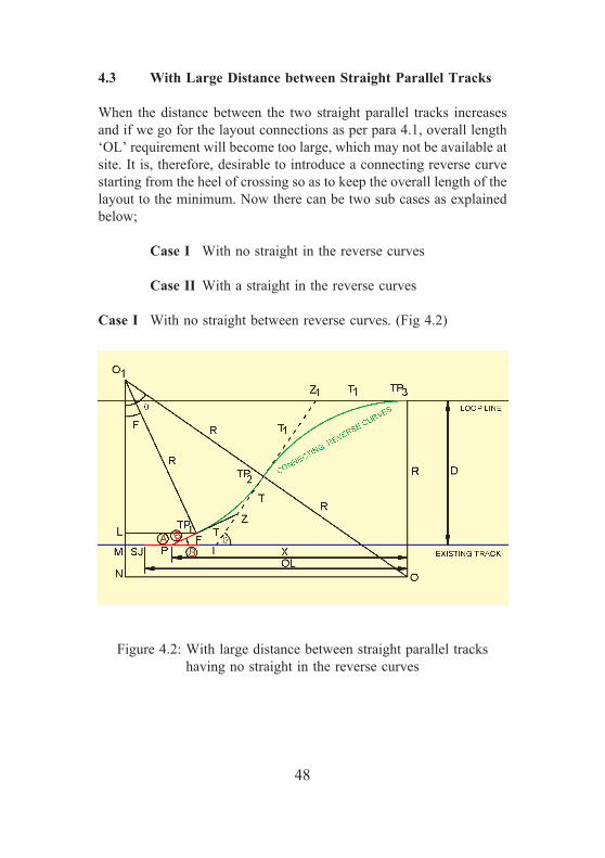
4.3 With Large Distance between Straight Parallel Tracks

When the distance between the two straight parallel tracks increasesand if we go for the layout connections as per para 4.1, overall length‘OL’ requirement will become too large, which may not be available atsite. It is, therefore, desirable to introduce a connecting reverse curvestarting from the heel of crossing so as to keep the overall length of thelayout to the minimum. Now there can be two sub cases as explainedbelow;

Case I With no straight in the reverse curves

Case II With a straight in the reverse curves

Case I With no straight between reverse curves. (Fig 4.2)

Figure 4.2: With large distance between straight parallel trackshaving no straight in the reverse curves

49

Formulae

Interpretation of Formulae and Field Practicalities

First of all, value of radius of connecting curve is to be assumed, whichis generally the same as that the radius of lead curve. Distance ‘D’ willbe known from the field. Value of various turnout parameters will beknown once we have decided the type of turnout.

Now from Eq 4.5, value of ‘θ’ will be calculated. Then from Eq 4.6 &4.7, tangent lengths ‘T’ & ‘T1 will be calculated. Value of ‘X’ andfinally ‘OL’ will be calculated from Eq 4.8 & 4.9 respectively. Nowwith respect to ‘TP3’, the location of ‘SJ’ can easily be fixed which willbe at a distance equal to ‘OL’. (Fig 4.2)

In the above case several variations can be made such as, different radiiof curvature for two legs of the reverse curve or a straight between the

{ }

1

1 1 1

1

1

-1

1

1 1

In Δ O NO

O N O M MN O L LM MNCosθ

O O 2R 2R

O L RCosF, LM BSinF, MN R-DRCosF BSinF R-D

Cosθ2R

RCosF BSinF R-D θ Cos (4.5)2R

θ FT Rtan (4.6)

2θ

T Rtan (4.7)2

X (B T)CosF (T T )Cosθ T (4.8)

OL X A

+ + += = =

= = =+ +

∴ =

+ +∴ =

−=

=

= + + + +

= + (4.9)

50

heel of crossing & start of the reverse curve. Various formulae asderived in the previous case can be modified as follows;

Figure 4.3

)R(R

D)-(RSinFS)(BCosFRCosθ

D-RMN SinF,S)(BLM CosF,LO

RR

MNLMLO

RR

MNMO

OO

NOCosθ

NOO ΔIn

21

12

11

21

1

21

1

1

1

1

2R

+

+++=∴

=+==

+

++=

+

+==

51

Purpose of these variations in the above formulae is to show that, byaltering one or other parameters, a layout connection can be designedto suit the diverse site conditions. Yard designer can design betterlayouts with this understanding. It is worth mentioning that, notrigonometrical formulae can solve a layout because of diverse siteconditions and variety of obligatory points. Several trial & errorcalculations will be required for designing an optimum layout.

{ }-1 2 1

1 2

2

1 1

1 1 1

R CosF (B S)SinF (R -D) θ Cos (4.10)(R R )

θ FT R tan (4.11)

2θ

T R tan (4.12)2

X (B T )CosF (T T )Cosθ T (4.13)

OL X A (4.14)

S

+ + +∴ =+

−=

=

= + + + + +

= +

52

Example 4.4

A BG track is required to be connected to a siding which is parallel at15m distance. By using a 52kg PSC, 1 in 8.5 turnout and the radius ofthe connecting curve being the same as that of the lead curve of 1 in 8.5turnout and without a straight between the reverse curve. Calculate therequired distances for the layout connection.

Given: F=6042’35”, D=15.000m, A=12.025m, B=16.486m,R=221.522

0 0

0 ' "

0 0

428.4520.967

2 221.522

RCosF BSinF R-D Cosθ

2R' " ' "221.522Cos6 42 35 16.486Sin 6 42 35 221.522 15.0

2 221.522

θ 14 45 37.2θ F

T Rtan2

' " ' "14 45 37.2 6 42 35 221.522 tan 15.588 m

2

=

=×

+ +=

+ + −=

×

∴ =−

=

−= =

0

1

1 1

' "θ 14 45 37.2T Rtan 221.522 tan 28.692 m

2 2X (B T) CosF (T T ) Cosθ T

(16.486 15.588) Co

= = =

= + + + +

= + 0 0' " ' "s 6 42 35 (15.588 28.692) Cos 14 45 37.2

28.692

31.854 42.819 28.692 103.365 m

OL X A 103.365 12.025 115.39 m

+ +

+

= + + =

= + = + =

53

Case II With a Straight between Reverse Curves

When as per Case I, it may be possible, that space available is less incomparison with what is required for making the connection thenoverall length ‘OL’ can be further reduced by introducing a straightbetween the reverse curve. In this Case, it is presumed that reversecurve is starting just after the heel of crossing.

Figure 4.4: With large distance between straight parallel trackshaving a straight in the reverse curve

Formulae

( )

1 2 3

2

1 2

1

In Δ O TP Z

TP Z S 2 S3tanψO TP R 2R

Sψ tan (4.15)2R

−

= = =

=

54

( )

( )

( )

(4.20)AXOL

(4.19)T)CosθTS(T)CosFT(BX

(4.18)2

θRtanT

(4.17)2

F-θRtanT

(4.16)2RS1tan

SSinψD-RBSinFRCosF

Cosθ

4.15, Eq from ψ'' of value thengsubstituti

ψS

SinψD-RBSinFRCosFCosθ

SSinψD-RBSinFRCosF

ψ)Cos(θ

Sinψ

SOO

OOS

OO

OOSinψ

OOO ΔIn

D-RMN BSinF,LM RCosF,LO

OO

MNLMLO

OO

MNMO

OO

NOψ)Cos(θ

NOO ΔIn

2211

2

1

1-

1-

21

2121

32

231

1

21

1

21

1

21

1

21

+=

+++++=

=

=

−−++

=

−++

=∴

++=+

=∴

==

===

++=

+==+

⎟⎠⎞

⎜⎝⎛

⎭⎬⎫

⎩⎨⎧

⎭⎬⎫

⎩⎨⎧

55

If we start the reverse curve after introducing another straight ‘S1’ afterthe heel of crossing and different degree of curvature of the two legs ofthe reverse curve (R1 & R2).

Figure 4.5

For the above variation (Fig 4.5) various formulae can be modified asexplained under.

[ ]

(4.25)AXOL

(4.24)TCosθ)TS(TCosF)TS(BX

(4.23)2

θtanRT

(4.22) 2

Fθ-tanRT

(4.21)RS

tanS

SinψD-RSinF)S(BCosFRCosθ

RRR e wherRS

tanψ

22111

22

11

12111-

211

+=

++++++=

=

=

−+++

=

+==

⎟⎠⎞

⎜⎝⎛

⎪⎭

⎪⎬⎫

⎪⎩

⎪⎨⎧

⎟⎠⎞

⎜⎝⎛

−

−

56

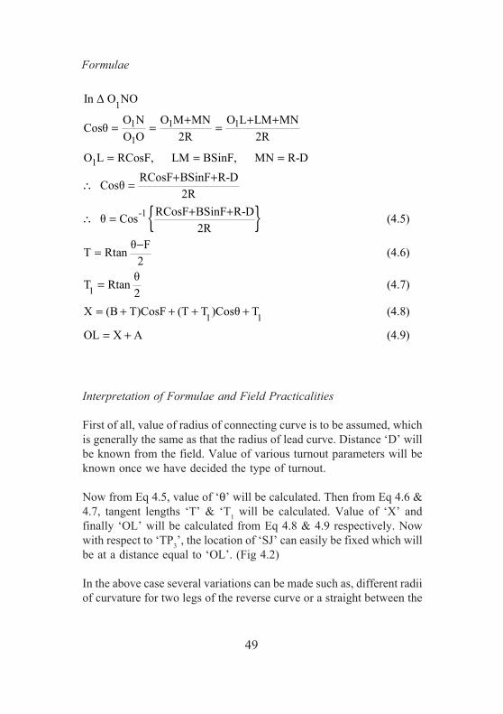
Example 4.5

In the Example 4.4, if a straight of 10m has to be introduced betweenthe reverse curves, the calculate the required distances for the settingthe layout.

( )( )

( )

( )( )

0 '

1

1 "

0 ' " 0 ' " 0 ' "

Sψ tan2R

10 0 ' tan 1 17 352 221.522

RCosF BSinF R-D SinψCos(θ ψ)

S

221.522Cos6 42 35 16.486Sin6 42 35 221.522-15 Sin1 17 35

10220.004 1.926 206.522 0.0225661

0.966810

1θ ψ Cos (0.99668) 14 47 3- -

−

−

=

= =×

+ ++ =

+ +=

+ + ×= =

−+ = = "

0 ' " 0 ' "

0 ' " 0 ' "

0 ' "

0 '

0 "

1

2

1 1 2 2

9.26'θ 14 47 39.26 1 17 35 13 30 42.6

θ-F 13 30 42.6 6 42 35T Rtan 221.522tan 13.144m

2 2

θ 13 30 42.6T Rtan 221.522tan 26.242m

2 2X (B T )CosF (T S T )Cosθ T

(16.486 13.144)Cos6 42 3

-= =

= = =

= = =

= + + + + +

= +

− − − − −

"

0 ' "

5

(13.144 10 26.242)Cos13 30 42.6 26.114

= 29.427 + 48.019 + 26.242 =103.688

OL X A 104.152 12.000 116.152m

= 103.688+12.025=115.713 mtr (Ans)

+ + +

= + = + =

+

57

Chapter 5

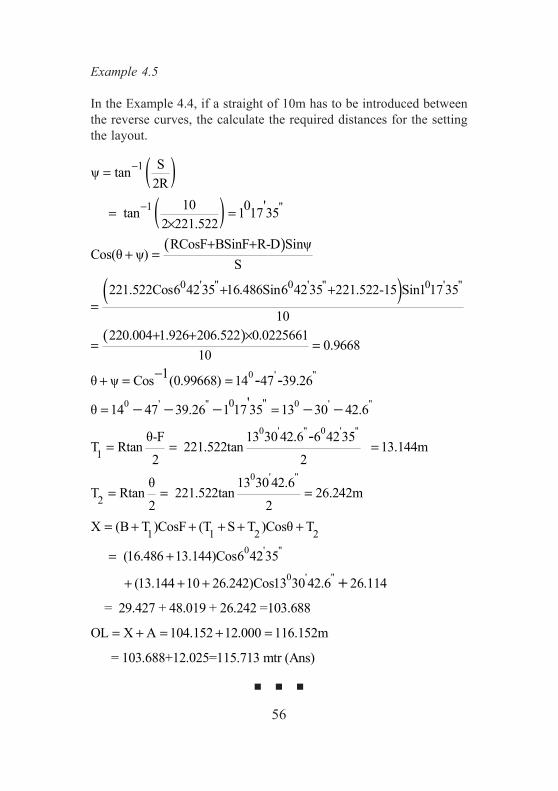
Crossover Connection between Straight Parallel Tracks

Type of Crossover connection between the straight parallel tracks will bedependent upon the distance between the two tracks and the spaceavailability. Accordingly distance between the two tracks may be treatedas Normal distance and Large distance. Concept of Normal distance andthe Large distance is not decided by the spacing between the two tracks,it is the arrangement of layout and accordingly trigonometric formulae.

5.1 With Normal Spacing between the Tracks and with Same Angleof Crossing

Figure 5.1: With normal spacing between the tracks andwith same angle of crossing

58

Formulae

Interpretation of Formulae and Field Practicalities

First of all the value of ‘D’ will be known from the field surveying. Turnoutprarmeters ‘A’, ‘B’ will be known once we have decided the type ofturnout. Then from Eq 5.2 & 5.3, the values of ‘X’ & finally ‘OL’ will becalculated. Now with these values in the hand, location of one of ‘SJ’ canbe fixed by keeping it at a distance ‘OL’ apart in refernce to another ’SJ’.After fixing the location of ‘SJ’, rest of the turnout can be set out by fieldsurveying.

For the correctness of the crossover connection, it is very important thatthe distance ‘D’ must be same in the vicinity of turnouts and must beaccurate. A small error in ‘D’ will get magnified by ‘N’(number of crossing)times. It is therefore very important that the value of ‘D’ must be arrivedat by field surveying and not from the yard drawings which might havebeen prepared long back and necessary corrections might not have beendone.

For example, if ‘D’ used for layout calculations is not equal to theactual distance available at the site, then two conditions may be thoughtof i.e;

Dcal<Dactualor

Dcal>Dactual

(B S B)SinF DD

S 2B (5.1)SinF

X DCotF DN (5.2)

where

+ + =

∴ = −

= =

N is the number of Xing. (CotF N )

OL X 2A (5.3)

=

= +

59

In both the cases, ‘SJ’ will be fixed wrongly and the connection, insteadof a straight,will become a reverse curve or a kink will be formed at theheel of crossing.

a) Dcal<Dactual

b) Dcal>Dactual

Figure 5.2

Now, when the train negotiate the crossover, it will try to straighten upthe reverse curve, which will finally result into alignment kink in the mainline and will result into bad running.

60

5.2 With Large Spacing between the Tracks with the SameAngle of Crossing

When the distance between the two straight parallel tracks increases andif we go for the layout connection as per para 5.1, overall length ‘OL’requirement will become two large, for which space may not be availableat the site. Space being the costly item in an yard, it is therefore desirableto introduce a connecting reverse curve starting ̀ from the heel of crossingso as to keep the overall length of the layout to the minimum. In this typeof layout, further there can be two sub cases i.e;

Case I With no Straight in the Reverse Curves

Case II With a given Straight in the Reverse Curves

Case I With no Straight in the Reverse Curves (Fig 5.3)

Figure 5.3: With no Straight between Reverse Curve

61

Formulae

Interpretation of Formulae and Field Practicalities

First of all, value of radius of connecting reverse curve is to be assumed,which is generally the same as that of lead curve radius of the turnout.Distance ‘D’ between the two straight parallel track will be known fromthe field. Value of turnout parameters will be known once we have decidedthe type of turnout.

Now from Eq 5.4, value of 'θ' can be calculated. Then from Eq 5.5, 5.6& 5.7, value of ‘T’, ‘X’ ann hence ‘OL’ can easily be calculatedrespectively. Now the location of ‘SJs’ can easily be fixed which willbe at a distance equal to ‘OL’.

[ ](5.7)2AXOL

(5.6)TCosθT)CosF(B2X

(5.5)2

F-θRtanT

(5.4)R

2DBSinFRCosF1Cosθ

R2D-BSinFRCosF

Cosθ

R2

TP1

O ,2DNM BSinF,LM RCosF,L1

O

TPO

NMLMLO

TPO

NMMO

TPO

NOCosθ

NTPO Δ

21

1

21

1

21

1

22

+=

++=

=

−+−=∴

+=∴

====

−+=

−==

⎟⎠⎞

⎜⎝⎛

62

In the above case, several variations can be made such as , different radiiof curvature of two legs of reverse curve or a straight between the heelof crossing and start of the reverse curve or different angle of crossing atthe two ends. (Fig 5.4)

Figure 5.4Formulae

In Δ O N TP1 1 2O N O M N M O L L M N M1 1 1 1 1 1 1 1 1 1 1 1CosθO TP O TP O TP1 2 1 2 1 2

O L R CosF , L M (B S )SinF , O TP R1 1 1 1 1 1 1 1 1 1 2 1R CosF (B S )SinF N M1 1 1 1 1 1 1 Cosθ

R1 N M R CosF (B S )SinF R Cosθ1 1 1 1 1 1 1 1

− + −= = =

= = + =

+ + −∴ =

∴ = + + −

63

Now, these formulae have become more versatile and generalized byincorporating these variations.

(5.12)2

A1

AXOL

(5.11)2

)CosF2

T2

S2

(B

)Cosθ2

T1

(T1

)CosF1

T1

S1

(BX

(5.10)2

2Fθtan

2R

2T

(5.9)2

1Fθtan

1R

1T

(5.8) 2R1R

D2)SinF2S2(B1)SinF1S1(B2CosF2R1CosF1R1-Cos

2R1R

D2)SinF2S2(B1)SinF1S1(B2CosF2R1CosF1RCosθ

D2

M2

N1

M1

N

Cosθ2

R2

)SinF2

S2

(B2

CosF2

R

Cosθ1

R1

)SinF1

S1

(B1

CosF1

R2

M2

N1

M1

N

Cosθ2

R2

)SinF2

S2

(B2

CosF2

R2

M2

N 2R

2M2N2)SinF2S2(B2CosF2RCosθ

2R

2TP

2O ,

2)SinF

2S

2(B

2M

2L ,

2CosF

2R

2L

2O

2TP2O2M2N2M2L2L2O

2TP2O2M2N2M2O

2TP2O2N2O

Cosθ

2TP

2N

2O ΔIn

++=

+++

++++=

−=

−=

+

−+++++=

+

−+++++=∴

=+

−+++

−++=+

−++=∴

−++=∴

=+==

−+=

−==

⎪⎭

⎪⎬⎫

⎪⎩

⎪⎨⎧

64

Example 5.1

A crossover is required to be laid between the two parallel BG tracks at15m distance by means of a 52 Kg, 1 in 12 turnout with no straightportion in the connection. Calculate the required parameters for thelayout. Also calculate the saving in overall length in this layout over alayout with straight line connection between the crossing.

Given: F=4045’49”, A=16.953m, B=23.981m, R=441.282m

[ ][ ]

48.559m165.347-213.906length overall in the saving Therefore

213.906m16.953212152ADCotFOL

crossing; the

between provided is connection linestraight iflength Overall

165.347m16.9532131.4412AXOL

131.441m20.779)2(44.941

"34'14021.116Cos14945421.116)Cos(23.9812

TCosθT)CosF(B2X

21.116m 2

49454-"34'1410tan441.282

2

F-θRtanT

341410θ

0.9840628441.282

215-494523.981Sin449454441.282CosCosθ

R2D-BSinFRCosF

Cosθ

0"'0

"'00

"'0

"'0"'0

==

=×+×=+=

=×+=+=

=+=

++=

++=

=

×=

=

=

=

+=

+=

65

Case II With a given Straight in the reverse curves

Figure 5.5 : With a given Straight in the reverse curve

Formulae

BSinF,NM RCosF,NO

ZO

LMNMNO

ZO

LM-MO

ZO

LOψ)Cos(θ

LZO ΔIn

(5.13)2RS

tanψ

2RS

R2S

TPO

ZTPtanψ

ZTPO ΔIn

1

1

1

1

1

1

1

1

1

21

2

21

==

−+===+

=

===

⎟⎠⎞

⎜⎝⎛−

66

( )

( )

( )

(5.17)2AXOL

(5.16)S)Cosθ(2TT)CosF2(B

B)CosF(TT)CosθS(TT)CosF(BX

(5.15)2

F-θRtanT

(5.14)2RS

tan

SSinψ2DBSinFRCosF2

Cosθ

ψS

Sinψ2DBSinFRCosF2Cosθ

SSinψ2D-RBSinFRCosF2

ψ)Cos(θ

2Sinψ

SZO

ZTPO ΔIn

1

1-

1-

1

21

+=

+++=

++++++=

=

−

−+×=∴

−−+×

=∴

++×=+

=

⎟⎠⎞

⎜⎝⎛

⎭⎬⎫

⎩⎨⎧

⎭⎬⎫

⎩⎨⎧

−

67

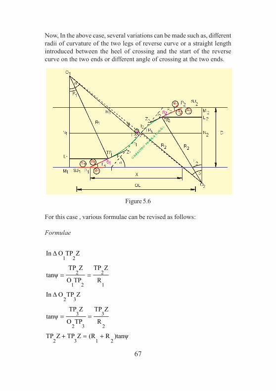
Now, In the above case, several variations can be made such as, differentradii of curvature of the two legs of reverse curve or a straight lengthintroduced between the heel of crossing and the start of the reversecurve on the two ends or different angle of crossing at the two ends.

Figure 5.6

For this case , various formulae can be revised as follows:

Formulae

)tanψR(RZTPZTP

R

ZTP

TPO

ZTPtanψ

ZTPO ΔIn

R

ZTP

TPO

ZTPtanψ

ZTPO ΔIn

2132

2

3

32

3

32

1

2

21

2

21

+=+

==

==

68

( )

( )

(-

ZO

ZTPSinψ

ZTPO ΔIn

OOZOZO where

(5.20a)ψ)Z)Cos(θOZO

)SinFS(B)SinFS(BCosFRCosFRD

MNMN D

ψ)ZCos(θO-)SinFS(BCosFR MN

ψ)ZCos(θO-)SinFS(BCosFR MN

5.20, & 5.19 Eq From

(5.20)ZO

MN-SinFS(BCosFRψ)Cos(θ

ZNO ΔIn

(5.19)ZO

MN-SinFS(BCosFRψ)Cos(θ

ZO

MN-MLLO

ZO

MN-MO

ZO

NOψ)Cos(θ

ZNO ΔIn

(5.18)2R1R

Stanψ

)R(R

S tanψ

S)ZTPZTP (where )tanψR(RS

1

2

21

2121

21

2221112211

2111

22222221

11111111

2

222)

2222

22

1

111)

1111

1

111111

1

1111

1

11

11

1-

21

3221

=

=+

++

+++++=

=

+++=

+++=

++=+

++=+

+===+

+=∴

+=∴

=++=

+

⎟⎟⎠

⎞⎜⎜⎝

⎛

69

Now these formulae have become more generalized by incorporatingthese variations.

[ ]

[ ]

(5.25)2AXOL

(5.24))CosFBS(T

)CosθTS(T)CosFTS(BX

(5.23)2

FθtanRT

(5.22)2

FθtanRT

(5.21)RR

Stan

S

SinψD2)SinF2S2(B1)SinF1S1(BCosF2RCosF1RCosθ

S

SinψD2)SinF2S2(B1)SinF1S1(BCosF2RCosF1R

: toequal is ψ)Cos(θ a), (5.20 Eq gconsiderin

SinψOOS

Z)SinψOZ(OZTPZTP

ZO

ZTPSinψ

ZTPO ΔIn

2222

211111

222

111

21

1

1

21

21

2132

2

3

32

+=

+++

+++++=

−=

−=

+−

−+++++=

−+++++=

+

=∴

+=+

=

⎟⎟⎠

⎞⎜⎜⎝

⎛

⎪⎭

⎪⎬⎫

⎪⎩

⎪⎨⎧

⎪⎭

⎪⎬⎫

⎪⎩

⎪⎨⎧

−

−

70

Example 5.2

A crossover is required to be laid between two parallel BG tracks at 15mdistance by means of 60Kg PSC, 1 in 12 turnout and with a straight of 40min connection. Calculate the required parameters for the layout. Alsocalculate the saving in overall length in this layout over a layout withstraight line connection between the crossing.

Given: F=4045’49” , A=16.989m, B = 22.912m, R = 400m, S = 40m

Overall length, if straight line connection is given between the crossing,

OL DCotF 2A 15 12 2 16.989 213.979m (When only straight)

Therefore saving in overall length 213.979 -167.153 46.82m

= + = × + × =

= =

( ) ( )( ){ }

( )

( )

1 1 0 ' "

-1

-1

0 ' " -1 0 ' "

S 40ψ tan tan 2 51 452R 2 4002 RCosF BSinF D 2 Sinψ

θ Cos ψS

0 ' " 0 ' " 0 ' "2 400Cos4 45 49 22.912Sin4 45 49 15 2 Sin2 51 45Cos

40

0 ' "2 398 1.902 15 2 Sin2 51 45 2 51 45 Cos 8 13 6.47

40

Cos

− −= = =×

× + −= −

× + −=

+ −− = =

=

⎧ ⎫⎪ ⎪⎨ ⎬⎪ ⎪⎩ ⎭

⎧ ⎫⎨ ⎬⎩ ⎭

{ }-1

0 ' "

0 ' "

0 ' ''2 51 45

0 0 ' '' 0 ' '' 0 ' ''4 51 47 2 51 45 8 13 6.47

39.2540

11 - =0 ' "θ - F 8 13 6 - 4 45 49

T Rtan 400tan 12.063m 2 2

X 2(B T)CosF (2T S)Cosθ 0 ' " 2(22.912 12.063)Cos4 45 49 (2 12.063 40)Cos8 13 6

−

− −=

= = =

= + + +

= + + × +

69.708 63.467 133.175m

OL X 2A 133.175 2 16.989 167.153m (When limited

straight 40 m consider)

= + =

= + = + × =

71

5.3 With Different Angles of Crossing and Normal Distancebetween the two Straight Parallel Tracks

Figure 5.7 : With different Angles of crossing and normal distancebetween the two straight parallel tracks

Formulae

(5.30)AAXOL

(5.29))CosFB(TT)CosF(BX

(5.28)2

2F1FRtanT

(5.27)2SinF1SinF

)2SinF2B1SinF1(B-DT

(5.26)D)SinFB(TT)SinF(B

21

2211

2211

++=

+++=

−=

+

+=∴

=+++

72

In the derivation of the various formulae for the above case, it is assumedthat connecting curve is starting just after the heel of crossing. It mayalso happen, to suit the varied site conditions, that a straight after theheel of crossing is required. Those formulae can be modified as follows;(Fig 5.8)

Figure 5.8

[ ]

(5.35)AAXOL

(5.34))CosFBS(TT)CosFS(BX

(5.33)2

2F1FRtanT

(5.32)2SinF1SinF

)2)SinFS2(B1SinFS(B-DT

(5.31)D)SinFBS(TT)SinFS(B

21

222111

2)

11

222111

++=

+++++=

−=

+

+++=∴

=+++++

73

Example 5.3

A crossover is required to be laid between the two straight parallel tracksat 4.725m centres by using a 52 Kg, 1 in 8.5 & 1 in 12 turnouts. Calculatethe required parameters for the layout.

Given: Turnout A B F

1 in 8.5 12.000m 17.418m 6042’35”

1 in 12 16.953m 23.981m 4045’49”

First of all, value of ‘T’ tangent length will be calculated from,

Note:

Radius of connecting curve, thus, coming is prohibitive for negotiatingthe passenger trains. It is recommended that radius of connecting curveshould be at least equal to the radius of lead curve of 1 in 12 turnout,which can be taken as 440m.

205.597m

2

"49'4504"35'4206tan

3.492

2

FFtan

T R

3.492m0.19988

1.992)(2.035-4.725

"49'450Sin4"35'420Sin6

)"49'45023.981Sin4"35'4206(17.418Sin-4.725

SinFSinF

)SinFBSinF(B-D T

21

21

2211

=−

=−

=

=+

=

+

+=

+

+=

74

Example 5.4

In the foregoing example 5.4, if the radius of connecting curve radius isrequired to be the same as that of the radius of lead curve of 1 in 12turnout, calculate the minimum distance ‘D’ between the two tracks andthe various parameters for the layout. Radius of connecting curve can betaken as equal to 441.282m.

21

2211

77.098m16.95312.00048.145

AAXOL

48.145m27.37820.767

"49'4503.492)Cos4(23.981 "35'4203.492)Cos6(17.418

)CosFB(TT)CosF(BX

=++=

++=

=+=

+++=

++++=

21

2211

2211

21

85.062m16.95312.00056.110

AAX OL

56.110m31.36724.742

"49'4504 7.495)Cos(23.981"35'4207.495)Cos6(17.418

)CosFB(TT)CosF(B X

5.525m2.6142.911

"49'45047.495)Sin (23.981"35'4207.495)Sin6(17.418

)SinFB(TT)SinF(B D

7.495m2

"49'4504"35'4206tan441.282

2

FFRtan T

=++=

++=

=+=

+++=

+++=

=+=

+++=

+++=

=−

×=−

=

Ans : Hence D= 5.525m when minimum connecting curve radius is takenon 441 mtr.

75

Example 5.5

In the foregoing example 5.4, if the layout is on PSC sleepers, thencalculate the minimum distance ‘D’ between the two tracks and otherparameters for correctly laying the layout in the field. Minimum radiusof connecting curve to be taken as that of the lead curve radius of 1 in12 turnout.

Given: Turnout A B F

1 in 8.5 12.025m 16.486m 6042’35”

1 in 12 16.989m 22.912m 4045’49”

(These turnout parameters are for PSC layouts, 1673mm Gauge)

For the PSC Fan Shaped Layout, the layout becomes rigidly straight upto the last common PSC sleepers(S.No 83 for 1 in 12, & S.No 54 for 1 in 8.5)of the turnout due to the prepositioned inserts for straight alignmentbehind the heel of crossing. These straight for 1 in 8.5 & 1 in 12 turnoutsare 3.3m & 5.688m respectively.

92.078m16.98912.02563.064AAX OL

63.064m35.97027.094 "49'4505.688)Cos422.912(7.495

"35'4203.3)Cos616.486(7.495 X

6.185m2.9983.187 "49'4505.688)Sin422.912(7.495

"35'4203.3)Sin616.486(7.495

)SinFBS(TT)SinFS(B D

7.495m2

"49'454"35'426tan441.282

2

FFRtan T

21

222111

0021

=++=++=

=+=+++

++=

=+=+++

++=

+++++=

=−

×=−

=

76

Note:

It is therefore, very important that when yard layout is on PSC FanShaped layout and track centre is less, then section engineer shouldremove long common sleepers from the Fan Shaped layout so that theconnecting curve can be started earlier. It may also happen that, whileperforming the layout calculations, default straight behind the heel ofcrossing might not have been taken into consideration and thereforeduring laying the turnout, geometry of the layout will be disturbedbecause of mismatch of calculations and the actual site parameters.Because of this mismatch, alignment will become kinky in the connectingcurve, which in turn will be reflected as the kink in main line.

5.4 Crossover between a Loop Line and the Main Line with theSymmetrical Split on the Loop Line

Figure 5.9 : Crossover between a loop line and the main line with thesymmetrical split on the loop line

77

Formulae

Interpretation of Formulae and Field Practicalities

From the field, value of ‘D’ will be known. Radius of connecting curvewill be assumed as per the guidelines. From Eq 5.37 value of ‘T’ can becalculated and the from Eq 5.36, 5.38 & 5.39, valus of ‘S’, ‘X’ & ‘OL’ canbe calculated respectively. Now the work left is locating one Stock Jointwith respect to another by keeping it at a distance ‘OL’ apart.

The same formulae can be used differently, when ‘S’ is given. Then fromEq 5.36 value of ‘T’ can be calculated and then from Eq 5.37, value of ‘R’can be calculated. Value of ‘R’ thus arrived may or may not satisfy therecommended radius of connecting curve.

Several variations can also be thought of like a straight after boththe Turnouts or a reverse curve between the heel of crossing. Purposeof incorporating these variations is basically for designing an optimumlayout keeping in view the space constraints, infringements or obligatorypoints.

(5.39)AAXOL

(5.38)2

F)CosB(TT)CosFS(BX

(5.37)2

2

FF

RtanT

(5.36)T)(B-SinF

2

FT)Sin(B-D

S

D22F

)SinB(TT)SinFS(B

21

2211

21

11

22

211

++=

++++=

−

=

++

=∴

=++++

⎟⎟⎠

⎞⎜⎜⎝

⎛

78

Example 5.6

A crossover is required to be laid between a Loop Line and a parallelmain line at 4.725m track centres by using a 52 Kg PSC, 1 in 8.5 symmetricalsplit turnout on the Loop Line and 52Kg PSC, 1 in 12 turnout on the mainLine. Radius of the connecting curve being equal to the lead radius of the1 in 8.5 symmetrical split. Calculate the required parameters for the layout.

Given: Turnout A B F

1 in 8.5 12.025m 16.4486m 16042’35”

1 in 12 16.989m 55.914m 4045’49”

Radius of the connecting curve will be ‘R’=443.882m

22

11

2 1 1 2

F2F1 2

0 ' "6 42 350 ' "4 45 492

T Rtan 443.882 tan 5.457m 2 2

FD-(B T)Sin2S - (B T)

SinF0 ' "6 42 354.725-(16.486 5.457)Sin

2 - (22.914 5.457) 13.089m 0 ' "Sin4 45 49F

X (B S T)CosF (T B )Cos2

(

⎛ ⎞−⎜ ⎟⎝ ⎠

−

= = × =

+= +

+= + =

= + + + +

=

⎛ ⎞⎜ ⎟⎝ ⎠

1 2

0 ' "6 42 350 ' "22.914 11.349 5.457)Cos4 45 49 (5.457 16.486)Cos2

39.609 21.905 61.515m

OL X A A 61.515 16.989 12.025 90.529m

+ + + +

= + =

= + + = + + =

79

5.5 Crossover in Multi Track Area

Crossover in Multi Track area known as ‘Double Junctions’ involveprovision of a diamond crossing in between two Turnouts. Such layoutspermit diversion of UP/DN directional train from fast corridor to theslow corridors and vice versa. The turnouts are normally of 1 in 12spread, while the diamond crossing is of 1 in 8.5 spread. Hence theconnection will involve a connecting Curve.

It will be seen that for such a connection, the minimum track centredistance required for introducing a connecting curve of 1 in 12 turnoutlead curve radius is 5.5m on BG which is not always available. The followingalternatives are recommended in such layouts;

• At locations where such layouts are already laid with theexisting distance between track centres , it is preferable toreplace the existing 1 in 12 turnout with 1 in 8.5 turnout withcurved switches to have a straight line connection i.e. without acurve between the heel of crossings. This will not only improvethe layout alignment but also result in saving in the overalldistance which may be of a great advantage in the restrictedsuburban area. If the replacement as suggested above can notbe effected for some reason or other, then existing layout can beimproved by correctly calculating the resultant radius ofconnecting curve after properly assessing the track centresdistance and providing the same with accuracy and care.

• Whenever such crossovers are newly introduced, intermediatediamond crossings should be of the same spread as that of theturnout. Therefore, for 1 in 12 turnout, the diamond crossing inbetween shall be of movable type so that the connection willbe by means of straight line connection between the heel ofcrossings.

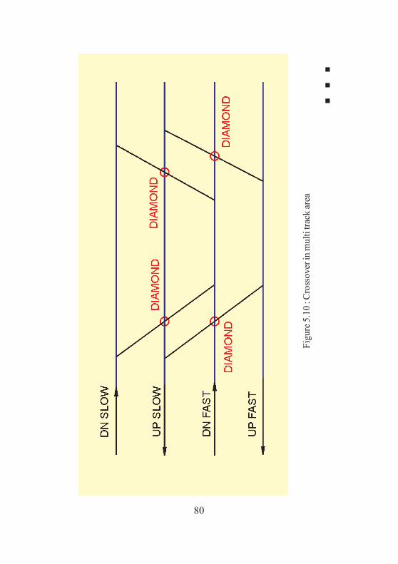
80

Figu

re 5

.10

: Cro

ssov

er in

mul

ti tra

ck ar

ea

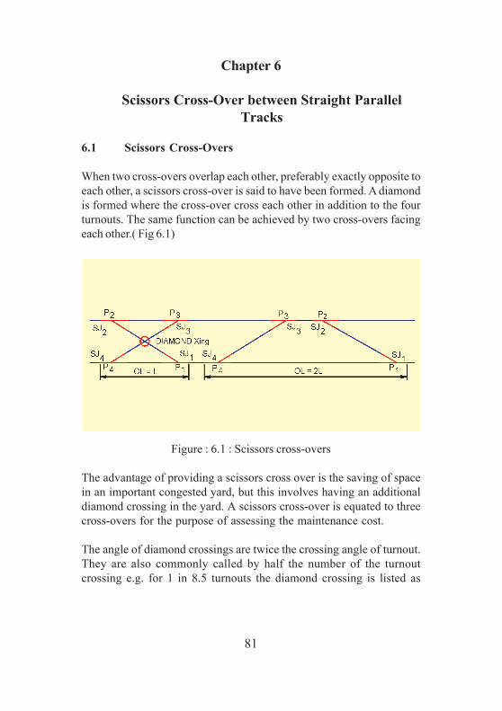
81

Chapter 6

Scissors Cross-Over between Straight ParallelTracks

6.1 Scissors Cross-Overs

When two cross-overs overlap each other, preferably exactly opposite toeach other, a scissors cross-over is said to have been formed. A diamondis formed where the cross-over cross each other in addition to the fourturnouts. The same function can be achieved by two cross-overs facingeach other.( Fig 6.1)

Figure : 6.1 : Scissors cross-overs

The advantage of providing a scissors cross over is the saving of spacein an important congested yard, but this involves having an additionaldiamond crossing in the yard. A scissors cross-over is equated to threecross-overs for the purpose of assessing the maintenance cost.

The angle of diamond crossings are twice the crossing angle of turnout.They are also commonly called by half the number of the turnoutcrossing e.g. for 1 in 8.5 turnouts the diamond crossing is listed as

82

1 in 4.25, though it is strictly incorrect because cot (2F) will not be halfthat of cot (F). On Broad Gauge, scissors cross-over layouts have beenfinalized only for two track centers (on wooden layouts) viz: 4.725 m(15’6”) and 5.180 m (17’0”). They can not be laid at track centers inbetween these distances due to difficulty in providing effective checkrail guidance over the unguided gap in front of the ANCs of acutecrossings for a wheel movement over the cross-overs.

6.2 Broad Gauge Scissors Cross-Over at 4.725m TrackCenters

At 4.725 m track centers, the distance between the TNCs of the acutecrossings of the diamond (Ld) formed in between the tracks is greaterthan the distance between the TNCs of the main line acute crossings (X).Hence the acute crossings of diamond lie outside the acute crossing ofthe main line turnouts as can be seen from the Fig 6.2.

Figure : 6.2 : Broad gauge scissors cross-over at 4.725m track centers

The distances involved for negotiating 1 in 8½ crossovers at 4.725 mtrack centers are as under-

83

The distance 1377 mm includes two gaps of 496 mm and 248 mm in frontof 1 in 8.5 and 1 in 4.25 acute crossings respectively, which are requiredto be protected by provision of check rails opposite them. Since thedistance between ANCs (X3) i.e. 1377 mm is greater than total unguidedgap (744 mm) at 4.725 m track centers, it is possible to provide specialcheck rails for guiding the movement of wheels along the cross-over.

As the track center distance increases the distance between TNCs ofmain line turnouts (X) also increases while the dimensions of thediamond (Ld) remains constant with the result that the distance betweenANCs of the acute crossings of main line and diamond (X2 and X3) getprogressively reduced making it difficult to provide check rails oppositeunguided gap. If the distance (X3) comes closer to 744 mm, the totalunguided gap, or lower than 744 mm then provision of check rail is notpossible. This aspect would be clear from the following table 6.1 for 1 in8.5 scissors cross-overs.

1377mmGtanF-CosF

1563 X

),(Xover -cross over the moving vehicleaby traversed

be wouldasover -cross thealong ANCsbetween distance The

1563mm4.25)in 1for ( 59 8.5)in 1for ( 1181386X

, )(Xstraight thealong ANCsbetween Distance

1386mm2

X-Lis )(X diamond and linemain

on crossings acute theof TNCs ebetween th distance Hence

14345mmSinF

GL

),(L diamond theof diagonal long The

11572mm 2F

GCot-DCotFX

(X), linemain on crossings of TNCsbetween Distance

3

3

2

2

d1

d

d

==

=++=

==

==

==

84

Table : 6.1D 4725 4800 4900 5000 5015 5100 5200 5300

X 11572 11210 13060 13910 14037 14760 15610 16460

Ld 14344 14344 14344 14344 14344 14344 14344 14344

X1 1386 1067 642 217 153 -208 -633 -4158

X2 1563 1244 819 394 330 -31 -456 -881

X3 1377 1056 628 200 136 -228 -656 -1084

As the track center increases the position becomes safe when ANCs ofthe diamond and ANCs of the main line crossings fall opposite eachother i.e. when distance X2 becomes zero ( Fig 6.3). This occurs whenthe track centers become 5.015 m beyond which the wing rails of thecrossing on main line and that of acute crossing of than diamond can beso extended that they perform the function of check rail opposite thecrossings and give the effective guidance. This is possible till suchincreased track center is obtained when independent check rails can beplaced opposite the respective gaps. The position is identicalwith 1 in 12 and 1 in 16 turnouts.

Figure : 6.3

85

For this purpose, Indian railways have finalized standard designsfor 4.725 m (15’6”) and 5.18 m (17’) track centers on wooden layoutswith extended wing rails for use on all new constructions. The designfor 4.725 m track center is to cover existing situation since majority ofthe yards are laid at 4.725 (15’6”) track centers.

A design for scissors cross-over on concrete sleeper layout at 4.725mtrack centre has been finalized for use in the field. However no design hasbeen finalized for 5.18m track centres on concrete sleepers.

No designs have been finalized for 5.3 m track center which is now therecommended track center for new constructions because as per therecommended guidelines, use of scissors cross-over is to be avoidedand on new constructions, layouts should be designed with the use ofnormal cross-overs.

For the Meter Gauge, effective independent check railing arrangementsare possible even when they are laid at 4.265 m track centers as thedistances between the TNCs are 5317 mm and 7548 mm in the case of 1 in8.5 and 1 in 12 scissors cross overs respectively. This is large enough toplace indepent checkrails opposite the nose of crossings.

86

Chapter 7

Crossovers between Non Parallel Straight Tracks

7.1 Crossovers between Non Parallel Straight Tracks

In the field, several situatios may arise where crossovers are to be laidbetween two non parallel straight tracks. Depending upon the siteconditions, variety of connections can be made like with same ordifferent angle of crossing, connecting curve being simple or reversecurve starting just after the heel of crossing or after a straight behindthe heel of crossing. If the connecting curve being the reverse curvethen it may be with or without a straight in between. It means that,there can be several permutations & combinations and variety offormulae can be generated.

Let us derive the set of formulae for a crossover connection between twonon parallel straight tracks with the following conditions;

Connecting curve being simple circular curve between the heel ofcrossing and angle of crossings being different on the two ends.

Figure 7.1 : Crossover between non parallel straight tracks

87

Formulae

Interpretation of Formulae and Field Practicalities

Given ‘R’, Angle between two non parallel straight tracks ‘ΔΔΔΔΔ’ andturnout parameters;

Eq 7.1 will be used for calculating the value of ‘T’. Once ‘T’ is known,Min ‘D’ (Where ‘SJ2’ will be fixed) will be calculated from Eq 7.2 andfinally ‘X’ & ‘OL’ will be calculated from Eq 7.3 & 7.4 respectively.Now ‘SJ1’ can be fixed at a distance ‘OL’ from ‘SJ2’.

Given ‘D’(where‘SJ2’ is fixed), Angle between two non parallel straighttracks ‘ΔΔΔΔΔ’ and turnout parameters;

Eq 7.2 will be used for calculating the value of ‘T’. Once ‘T’ is known,value of ‘R’ can be calculated from Eq 7.1 which may or may notsatisfy the recommended radius of turn-in-curve. After that the value of‘X’ & ‘OL’ can be calculated from Eq 7.3 & 7.4 respectively.

(7.4)CosΔAAXOL

(7.3)Δ)-)Cos(FB(TT)CosF(BX

(7.2)DSinΔAΔ))Sin(FB(TT)SinF(B

(7.1)2

FFΔRtanT

21

2211

22211

21

++=

+++=

=−+++

−+=

−

88

Example 7.1

A crossover consisting of 52 Kg, 1 in 12 and 1 in 8.5 turnouts isrequired to be laid between non parallel straight tracks at a minimumdistance between the two track centres. The angle between he two nonparallel straight tracks is 3050’0”. Calculate the various parametersrequired to lay the crossover connection assuming the connecting curveradius equal to 400m.

Given: Turnout A B F

1 in 8.5 12.000m 17.418m 6042’35”

1 in 12 16.953m 23.981m 4045’49”

110.432m"0'50016.953Cos312.00081.517

CosΔAAXOL

81.517m44.16637.351

)"0'5003"49'450(423.981)Cos(20.191

"35'420620.191)Cos(17.418

Δ)-)Cos(FB(TT)CosF(BX

3.978m1.133-0.7174.394

"0'50016.953Sin3 )"0'5003"49'450(423.981)Sin(20.191

"35'420620.191)Sin(17.418

SinΔAΔ))Sin(FB(T"35'420T)Sin6(BDmin

20.191m2

"49'4504"35'4206"0'5003tan400

2

FFΔRtanT

21

2211

2221

21

=++=

++=

=+=

−++

+=

+++=

=+=

−−++

+=

−+++=

=−+

×=

−+=

−

89

Chapter 8

Connection between Curved Track to Parallel CurvedTrack or Divergent Straight Track

Connections have at times to be laid from Curved Track to eitherparallel track or divergent straight track. Understanding about suchconnections is very important for a field engineer so that the same canbe applied for proper design of such layouts. Several situations can bethought of such that;

• Connection between two curved parallel tracks. Connectionbeing on outside of main Line curve without a straight betweenthe heel of crossing and the connecting curve.

• Connection between two curved parallel tracks. Connectionbeing on outside of main Line curve with a straight between theheel of crossing and the connecting curve.

• Connection between two curved parallel tracks. Connectionbeing on inside of main Line curve

• Connection between a curved track to straight track, theintersection being on the inside of the main line curve.

• Connection between a curved track to straight track, theintersection being on the outside of the main line curve.

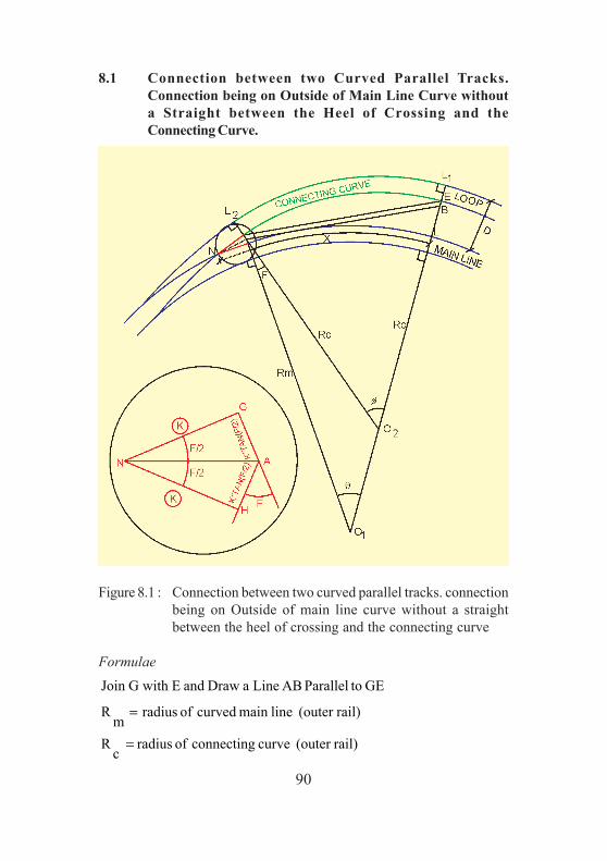
90

8.1 Connection between two Curved Parallel Tracks.Connection being on Outside of Main Line Curve withouta Straight between the Heel of Crossing and theConnecting Curve.

Figure 8.1 : Connection between two curved parallel tracks. connectionbeing on Outside of main line curve without a straightbetween the heel of crossing and the connecting curve

Formulae

rail)(outer curve connecting of radius c

R

rail)(outer linemain curved of radius m

R

GE toParallel AB Line a Draw and EG with Join

=

=

91

2F

2Ktan-G-D

2F

Ktanm

R2F

Ktan-G-Dm

RA O-BO

2F

Ktanm

RHAHOAO

2

FKtanGAEB where

2F

Ktan-G-Dm

REB-EL-LOBO

FAOO

A) B OBA O (where BA O-BA OAOO

BAO-BA OAOOA BO-BA O

2

B OA Cot

AOBO

AOBO

2

A BO-BA Otan

Formula, tan Applying B,A O ΔIn

GE) toParallel is (ABBA O BA O

G EO EG O

Triangle) (IsocelesEG O ΔIn

FAOO

8.1, Fig theofGeometry theFrom

11

11

1111

21

212221

122111

1

11

1111

1

22

22

2

21

=

−−+=∴

+=+=

==

+==

=∠=

∠=∠∠∠+∠=

∠∠+∠=∠∠

∠

+

−=

∠∠

∠=∠∴

∠=∠

=∠

92

2F

KtanGcR

Sinθ

2F

Ktanm

R

φ)-Sin(180

2F

KtanGc

RGA-GL-LOAO

2F

Ktanm

RAO

A O2O 1OA Sin

A O

AO OSin

Formula, SineApply OA O Δ

(8.1)2F

CotG-Dm2R

2F

2Ktan-G-D2tanθ

2F

CotG-Dm2R

2F

2Ktan-G-D

2θ

tan

2θ

CotG-Dm2R

2F

2Ktan-G-D

2F

tan

G-Dm

2R 2F

Ktanm

R2F

Ktan-G-Dm

RA OBO

2222

1

21

21

21

1-

11

−−=

+∴

−−==

+=

∠=

∠

⎟⎟⎟⎟

⎠

⎞

⎜⎜⎜⎜

⎝

⎛

+=∴

+=∴

+=∴

+=

+++=+

⎪⎭

⎪⎬

⎫

⎪⎩

⎪⎨

⎧

⎟⎟⎟⎟

⎠

⎞

⎜⎜⎜⎜

⎝

⎛

⎟⎟⎟⎟

⎠

⎞

⎜⎜⎜⎜

⎝

⎛

93

Interpretation of Formulae and Field Practicalities

When the connections pertaining to curved lines are required to be laidin the field, it will be prudent to fix the crossing first and then the entireturnout and connecting curves are being laid.

Distance ‘D’ between the two curved parallel tracks and radius of mainline ‘Rm’ will be known from field surveying. Value of turnout parameterswill be known once we have decided the turnout.

Now from Eq 8.1, value of ''θ will be calculated. Eq 8.2 will be used forcalculating the value of radius of connecting curve ‘Rc’. And Finally ‘X’will be calculated from Eq 8.3. Point ‘L1’ and hence Point ‘L’ will bedecided from field surveying. Now with refernce to ‘L’, distance ‘X’ willbe measured along the outer rail of curved main line to fix the TNC. It mayalso happen that TNC is already fixed, then Point ‘L’ can be fixed bymeasuring a distance ‘X’ along the outer rail of the curved main line.After ‘L’ being fixed, ‘L1’ can easily be fixed by field surveying.

It is evident from the formulae, that value of connecting curve radius ‘Rc’will be fixed for a given set of boundary conditions like ‘Rm’, ‘D’ &turnout parameters. It may so happen that ‘Rc’ may or may not satisfy therecommended radius of connecting curve.

(8.3) degreesin is θ'' e wher180

θmRK

radiansin is θ'' re wheθm

RKHLNHX

(8.2)2F

KtanGF)Sin(θ

2F

KtanmRSinθ

cR

Fθφ e wher

2F

KtanGcR

Sinθ

2F

Ktanm

R

F)Sin(θ

π

+=

+=+=

+++

⎟⎟⎠

⎞⎜⎜⎝

⎛+

=∴

+=−−

=+

+

94

Example 8.1

Calculate the radius of connecting curve ‘R’ and layout distance ‘X’ fora connection between a curved main line and a curved parallel track at4.725m distance. Connection being on the side of the main line withouta straight after the heel of crossing by using 1 in 8.5 crossing.

Given; K=3.123m, F=6042’35”, R=450m

48.877m180

"33'4905 4503.123

180

θmRK X

212.395m2

"35'4206tan3.1231.676

)"35'4206"33'490Sin(5

2

"35'4206tan3.123450"33'490Sin5

2F

KtanGF)Sin(θ

2F

KtanmRSinθ

cR

"33'4905903.049

17.05892.6828572tan

2

"35'4206Cot

1.676-4.725-45022

"35'42063.123tan2-1.676-4.725

2tan

2F

CotG-Dm2R

2F

2Ktan-G-D2tanθ

π π

1-

1-

1-

=×

+=+=

=×++

+

⎟⎟⎟

⎠

⎞

⎜⎜⎜

⎝

⎛×+×

=

+++

⎟⎟⎠

⎞⎜⎜⎝

⎛+

=

=×=

⎟⎟⎟⎟⎟

⎠

⎞

⎜⎜⎜⎜⎜

⎝

⎛

×

×=

⎟⎟⎟⎟

⎠

⎞

⎜⎜⎜⎜

⎝

⎛

+=

×

⎟⎠⎞⎜

⎝⎛

⎪⎪⎭

⎪⎪⎬

⎫

⎪⎪⎩

⎪⎪⎨

⎧

⎪⎭

⎪⎬

⎫

⎪⎩

⎪⎨

⎧

95

Note:

Calculations as performed above are the direct calculations. But incase of designing a layout connection, limiting the radius of theconnecting curve ‘Rc’, it will be required to calculate the requiredradius of curved main line so as to satify the predecided radius ofconnecting curve. For such calculations, problem can best be solved by‘Trial & Error’ process with a number of values of ‘Rm’. A ready madegraph can also be prepared between ‘Rm’ & ‘Rc’ for different trackcentres for a given turnout, connection being on outside of main linewithout a straight after the heel of crossing.

96

8.2 Connection between two curved parallel tracks.Connection being on outside of main Line curve with astraight between the heel of crossing and the connectingcurve

The author is against this type of layout unless ‘D’ is very large asotherwise the ‘Rc’ is reduced considerably because of a straightbetween the heel of crossing and the connecting curve. For normaldistances of the loop line, the ‘Rc’ will have prohibitive values unless ‘D’is very very large. This layout as well as the layout discussed in previousclause, three curves i.e. lead curve, connecting curve & parallel curvedline are laid and for good maintenance, it is very much desirable to havethe curves as large as possible.

Figure 8.2:Connection between two curved parallel tracks. Connectionbeing on outside of main line curve with a straight betweenthe heel of crossing and the connecting curve.

97

2

cRG

2F

Ktan)CosF2F

Ktanm

(R

S)SinF2F

Ktanm(R)c

R-Dm

R

POPOOO

G)-c

(R2F

Ktan)CosF2F

Ktanm

(RPO

G)-c

(R-)CosF2F

Ktanm

(R2F

Ktan

)LLL(OAQGALOGQLOPLPO

tan S)SinF2F

Ktanm

(R

SASinFOQPQOPOc

R-Dm

R

OLLLLOOL-LOOO

O PO ΔIn

8.2, Fig theofGeometry theFrom

crossing of heel after theStraight S

rail)(outer curve connecting of Radius c

R

rail)(outer linemain curved of Radius m

R

GE toParallel AB Line a Draw and EG with Join

(

22

2121

22

2 1

221

2

4222424242

111

2111211121

21

⎭⎬⎫

⎩⎨⎧+

⎭⎬⎫

⎩⎨⎧

−+++

++=+

+=

−++=∴

++=

−−+=−=−=

+=++=

==+=+=

+=

−+==

=

=

=

Equation; above the in PO & POOO of values the ngSubstituti

2F

Km

RAO where

SGLQP where

,

1

4

Formulae

98

Interpretation of Formulae and Field Practicalities

Distance ‘D’ between the two curved parallel tracks and radius ‘R’ ofmain line will be known from field surveying. Value of turnout parameterswill be known once we have decided the type of turnout. Now value of‘S’ will have to be assumed. Then from Eq 8.4 value of ‘Rc’ will becalculated. Value of ‘ϕ’and finally ‘X’ can be calculated from Eq 8.5 & 8.6respectively. Now TNC can be fixed easily as discussed in the previousclause.

{ }(8.6)

180

φ)(F-90mRK

180

θmRKHLNHX

φ)(F-90θ hence & 18090φθFO AQ ΔIn

(8.5)cR-DmR

S)SinF2F

Ktanm(R

OO

POCosφ

(8.4)

2F

Ktan-G-)CosF2F

Ktanm(R-DmR2

2G

2F

Ktan)CosF2F

Ktanm(R-

2F

Ktan-G-)CosF2F

Ktanm(R-DmR2

2S)SinF

2F

Ktanm(RD)m(R

cR

cRfor solving now G

2F

Ktan)CosF2F

Ktanm(Rc

2R

cRG

2F

Ktan)CosF2F

Ktanm(R

S)SinF2F

Ktanm(Rc

D)Rm

R2c

RD)m

R

π π

((

,1

21

1

2

22

222

++=+=+=

+==+++

+

++==

++

⎭⎬⎫

⎩⎨⎧

+++

++

⎭⎬⎫

⎩⎨⎧

++−+=

+++−

+++++

++=+−++

⎭⎬⎫

⎩⎨⎧

⎭⎬⎫

⎩⎨⎧

⎭⎬⎫

⎩⎨⎧

⎭⎬⎫

⎩⎨⎧

⎭⎬⎫

⎩⎨⎧

99

Example 8.2

A curved main line track of 600m radius is required to be connected to aparallel siding at 4.725m distance on the outside by using a 60 Kg PSC,1 in 12 turnout and with a straight portion of 10m behind the heel ofcrossing. Calculate the various parameters for the layout.

Given: F=4045’49”, K=2.803m

{ }{ }

{ }{ }

20 ' "4 45 492 0 ' "(600 4.725) (600 2.803 tan ) Sin4 45 49 102

42 600 4.725 - (600 2.803 tan

22F(R D) (R Ktan )SinF Sm m 2Rc F F2 R D-(R Ktan )CosF-G-Ktanm m 2 2

2F F(R Ktan )CosF Ktan Gm 2 2- F F2 R D-(R Ktan )CosF-G-Ktanm m 2 2

+ − + × +

+ + ×

+ − + +=

+ +

+ + +

+ +

=

⎧ ⎫⎨ ⎬⎩ ⎭

0 ' " 0 ' "45 49 4 45 490 ' ") Cos4 45 49 -1.676 - 2.803 tan2 2

20 ' " 0 ' "4 45 49 4 45 490 ' "(600 2.803 tan )Cos4 45 49 2.803 tan 1.6762 2

0 ' " 0 ' "4 45 49 4 45 490 ' "2 600 4.725-(600 2.803 tan )Cos4 45 49 -1.676-2.803 tan2 2

-

×

+ × + × +

+ + × ×

⎧ ⎫⎨ ⎬⎩ ⎭

⎧ ⎫⎨ ⎬⎩ ⎭

⎧ ⎫⎨ ⎬⎩ ⎭

100

From the above examples, it is evident that introduction of straightbehind the heel of crossing is not desirable, since it reduces theradius of connecting curve.

F(R Ktan )SinF Sm 2CosφR D-Rm c

0 ' "4 45 49 0 ' "(600 2.803 tan )Sin4 45 49 102 0.15952055

600 4.7250 ' " 0 ' "φ 80 4915 , therefore θ 90 - (4 45 49 )

R (90-(F φ))mX K 180

600

180

π

π2.803

+ +=

+

+ × += =

+

∴ = =+

= +

= +×

= 13.280 m

101

8.3 Connection between two curved parallel tracks. Connectionbeing on inside of main Line curve

Figure 8.3 : Connection between two curved parallel tracks. Connectionbeing on inside of main Line curve

102

( )

GDm

2R2F

KtanDm

R2F

KtanGm

RBOAO

2F

2KtanGD

2F

KtanDm

R2F

KtanGm

RBO-AO

2F

KtanD-m

R EBLE-LOBO

2F

KtanGm

RHA-MHMOAO

F OA OBA O-A BO1OA 2O-BA 2O-A BOBA O-A BO

2θ

CotBOAO

BOAO

2

BA O-A BOtan

Formula, tan Applying B,A O ΔIn

GE) toParallel is (ABBA O BA O

B,A O ΔIn

G EO EG O Triangle) (IsocelesEG O ΔIn

8.3, Fig theofGeometry theFrom

rail)(outer curve connecting of radius c

R

rail)(outer linemain curved of radius m

R

GE toParallel AB Line a Draw and EG with Join

11

11

11

11

1222

111

1

1

1111

1

11

1

22

2

−−=+−+−−=+

−−=

−+−−−=

+=+=

−−=−=

=∠+∠∠=

∠∠∠=∠∠

+

−=

∠∠

∠=∠∴

∠=∠

=

=

Formulae

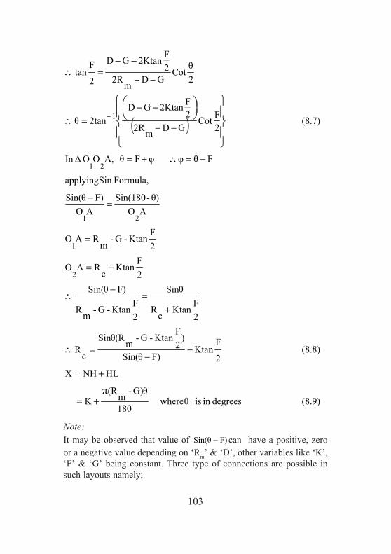
103

Note:It may be observed that value of F)Sin(θ − can have a positive, zeroor a negative value depending on ‘Rm’ & ‘D’, other variables like ‘K’,‘F’ & ‘G’ being constant. Three type of connections are possible insuch layouts namely;

( )

(8.9)degreesin is θ where180

G)θ-m(RK

HLNHX

(8.8)2

FKtan

F)Sin(θ

)2F

Ktan-G-mSin

cR

2F

KtancR

Sinθ

2F

Ktan-G-mR

F)Sin(θ

2F

Ktanc

RAO

2F

Ktan-G-m

RAO

AOθ)-Sin(180

AOF)Sin(θ

Formula,Sin applying

Fθφ φFθ A,OO ΔIn

(8.7)2FCot

GDm2R2F2KtanGD

2tanθ

2θ

CotGDm2R

2F

2KtanGD

2

F tan

π

2

1

21

21

1

+=

+=

−−

=∴

+=

−∴

+=

=

=−

−=∴+=

−−

−−=∴

−−

−−=∴

⎪⎭

⎪⎬

⎫

⎪⎩

⎪⎨

⎧ ⎟⎠⎞⎜

⎝⎛

−

R(θ

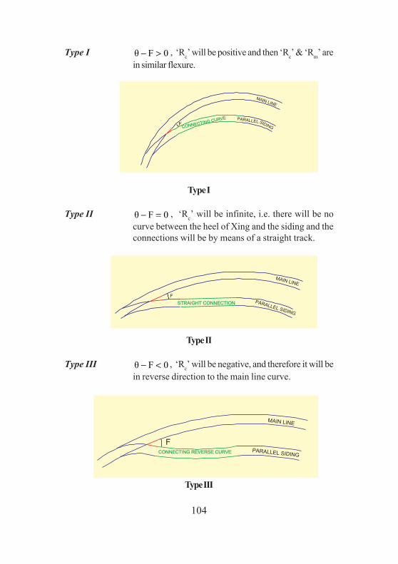
104

Type I θ F 0− > , ‘Rc’ will be positive and then ‘Rc’ & ‘Rm’ arein similar flexure.

Type I

Type II θ F 0− = , ‘Rc’ will be infinite, i.e. there will be nocurve between the heel of Xing and the siding and theconnections will be by means of a straight track.

Type II

Type III θ F 0− < , ‘Rc’ will be negative, and therefore it will bein reverse direction to the main line curve.

Type III

105

Example 8.3

A curved main line track of 500m radius is required to be connected toa curved parallel siding at 4.725m distance, the connection being on theinside of the curve by means of a 52 Kg, 1in 12 turnout. Calculate thevarious parameters for the layout.

Given: F=4045’49”, K=3.834m

( )

( )

69.574m180

"31'33071.676)-(5003.843

180

G)θ-m(RKX

1343.672m 2

"49'4504tan3.834

)"49'4504"31'330Sin(7

)2

"49'4504tan3.834-1.676-(500"31'330Sin7

cR

2

FKtan

F)Sin(θ

)2F

Ktan-G-mRSin

cR

I) (Type F"31'3307

2

"49'4504Cot1.6764.7255002

2

"49'4504Ktan3.83421.6764.725

2tan

2FCot

GDm2R2F

2KtanGD2tanθ

ππ

1

1

=×

+=+=

=×−

−

×=

−−

=

>

−−×

××−−

=

−−

−−=

=

⎪⎪⎭

⎪⎪⎬

⎫

⎪⎪⎩

⎪⎪⎨

⎧⎟⎟⎠

⎞⎜⎜⎝

⎛

⎪⎭

⎪⎬

⎫

⎪⎩

⎪⎨

⎧

⎟⎟⎟

⎠

⎞

⎜⎜⎜

⎝

⎛

−

−

(θ

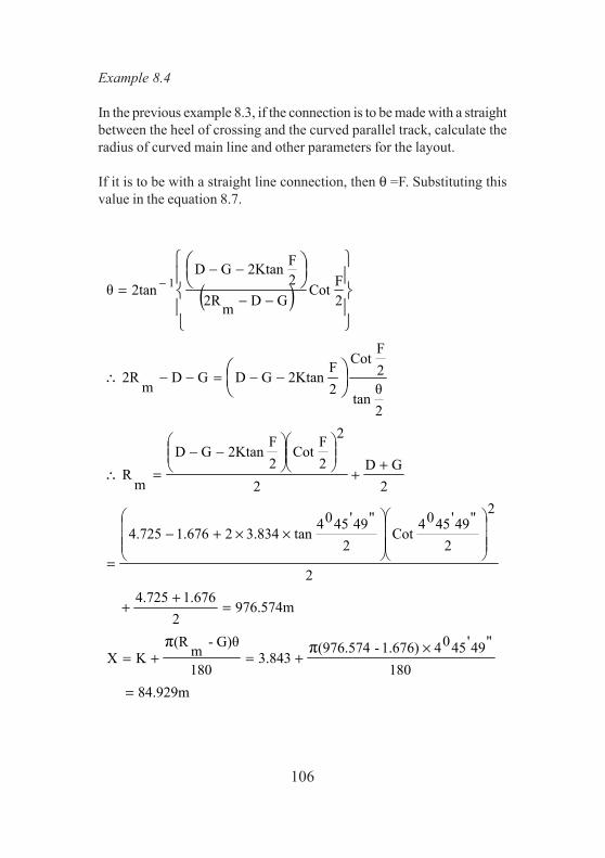
106

Example 8.4

In the previous example 8.3, if the connection is to be made with a straightbetween the heel of crossing and the curved parallel track, calculate theradius of curved main line and other parameters for the layout.

If it is to be with a straight line connection, then θ =F. Substituting thisvalue in the equation 8.7.

( )

84.929m 180

"49'45041.676)-(976.5743.843

180

G)θ-m(RKX

976.574m2

1.6764.725

2

2

2

"49'4504Cot

2

"49'4504tan3.83421.6764.725

2GD

2

2

2F

Cot2F

2KtanGD

mR

2θ

tan

2F

Cot

2F

2KtanGDGDm

2R

2FCot

GDm2R2F2KtanGD

2tanθ

ππ

1

=

×+=+=

=+

+

⎟⎟⎟

⎠

⎞

⎜⎜⎜

⎝

⎛

⎟⎟⎟

⎠

⎞

⎜⎜⎜

⎝

⎛××+−

=

++

⎟⎟⎠

⎞⎜⎜⎝

⎛⎟⎟⎠

⎞⎜⎜⎝

⎛−−

=∴

−−=−−∴

−−

−−=

⎟⎠⎞

⎜⎝⎛

⎪⎭

⎪⎬

⎫

⎪⎩

⎪⎨

⎧ ⎟⎠⎞⎜

⎝⎛

−

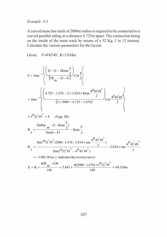
107

Example 8.5

A curved main line track of 2000m radius is required to be connected to acurved parallel siding at a distance 4.725m apart. The connection beingon the inside of the main track by means of a 52 Kg, 1 in 12 turnout.Calculate the various parameters for the layout.

Given: F=4045’49”, K=3.834m

( )

( )

69.510m180

"59'52011.676)-(20003.843

180

G)θ-m(RKX

curve) reverse theindicates (- 1306.381m

2

"49'4504tan3.834

)"49'4504"59'520Sin(1

)2

"49'4504tan3.834-1.676-(2000"59'520Sin1

cR

2

FKtan

F)Sin(θ

)2F

Ktan-G-mSinθin

cR

III) (Type F"59'5201

2

"49'4504Cot1.6764.72520002

2

"49'4504Ktan3.83421.6764.725

2tan

2FCot

GDm2R2F2KtanGD

2tanθ

ππ

1

1

=×

+=+=

−=

×−−

×=

−−

=

<

−−×

××−−

=

−−

−−=

=

⎪⎪⎭

⎪⎪⎬

⎫

⎪⎪⎩

⎪⎪⎨

⎧⎟⎟⎠

⎞⎜⎜⎝

⎛

⎪⎭

⎪⎬

⎫

⎪⎩

⎪⎨

⎧⎟⎠⎞⎜

⎝⎛

−

−

108

8.4 Connection between a curved track to straight track, theintersection being on the inside of the main line curve

+

Figure 8.4 : Connection between a curved track to straight track, theintersection being on the inside of the main line curve

109

Formulae

(8.10)CosFR2RRROO

CosFAOAO2-AOAOOO

formula Cosapply A,OO ΔIn

(say) R2F

Ktan-G-m

RGA-GL-LOAO

(say) R2F

Ktanc

RHAHOAO

rail)(outer curve connecting of radius c

R

rail)(outer linemain curve of radius m

R

212

22

12

21

212

22

12

21

21

21111

122

d

−+=∴

×××+=

===

=+=+=

=

=

(8.12)CosFR2RRR

G)CosΔ-m(R-cR

OO

LO Sinφ

G)CosΔ-m

(R-c

R

Q)CosΔL-L(O-c

R

QCosΔO-c

RPO-c

RLM-MOLO

,O LO ΔIn

(8.11)CosFR2RRR

SinFRSinθ

OO

SinF

AO

Sinθ

formula, Sine applying now

212

22

121

2

221

1122

21

212

22

1

1

212

−+==

=

=

===

−+=∴

=

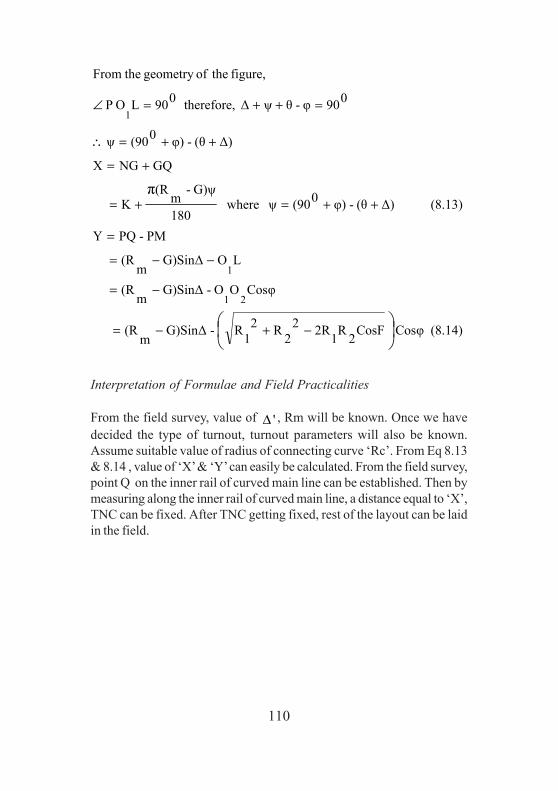
110

(8.14)Cosφ CosF2R12R22R2

1R-G)SinΔm

(R

CosφOO-G)SinΔm

(R

LOG)SinΔm

(R

PM-PQY

(8.13)Δ)(θ-φ)0(90ψ where180

G)ψ-m(RK

GQNGX

Δ)(θ-φ)0(90ψ

090φ-θψΔ e, therefor090LO P

figure, theofgeometry theFrom

21

1

1

π

⎟⎠⎞

⎜⎝⎛

−+−=

−=

−−=

=

++=+=

+=

++=∴

=++=∠

Interpretation of Formulae and Field Practicalities

From the field survey, value of 'Δ , Rm will be known. Once we havedecided the type of turnout, turnout parameters will also be known.Assume suitable value of radius of connecting curve ‘Rc’. From Eq 8.13& 8.14 , value of ‘X’ & ‘Y’ can easily be calculated. From the field survey,point Q on the inner rail of curved main line can be established. Then bymeasuring along the inner rail of curved main line, a distance equal to ‘X’,TNC can be fixed. After TNC getting fixed, rest of the layout can be laidin the field.

111

Example 8.6

A curved track of 450m radius is required to be connected to a straighttrack intersecting on the inside rail of the curved track at an angle of 500.The connection is to laid by means of 52 Kg, 1 in 12 turnout with aconnecting curve radius of 300m. calculate the various parameters for theturnout.

Given: F=4045’49”, K=3.834m

522835.0985

001.676)Cos5-(450-300 Sinφ

CosFR2RRR

G)CosΔ-m(R-cR Sinφ

"40'2909 θ

522835.0985

24.927

"49'450Cos4448.165300.1592448.165300.159

"49'450Sin4300.159

CosFR2RRR

SinFRSinθ

448.165m2

"49'4504tan3.834-1.676-450

2F

Ktan-G-m

RR

300.159m2

"49'4504tan3.834300

2F

Ktanc

RR

212

22

1

22

212

22

1

1

2

1

=

−+=

=∴

=

×××−+

×=

−+=

=×=

=

=×+=

+=

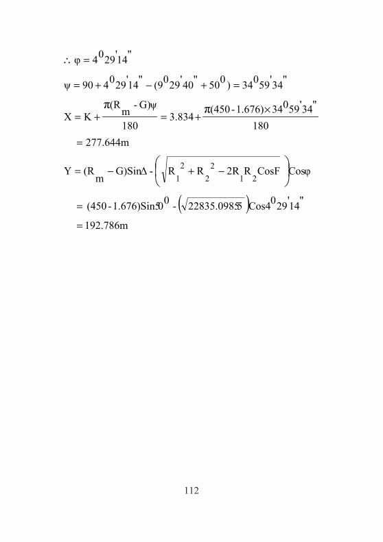
112

( ) 192.786m

"14'290Cos4 522835.0985 -001.676)Sin5-(450

Cosφ CosFR2RRR-G)SinΔm

(RY

277.644m 180

"34'590341.676)-(450 3.834

180

G)ψ-m(RKX

"34'59034)050"40'290(9"14'290490ψ

"14'2904φ

212

22

1

ππ

=

=

−+−=

=

×+=+=

=+−+=

=∴

⎟⎠⎞

⎜⎝⎛

113

8.5 Connection between a curved track to straight track, theintersection being on the outside of the main line curve

Figure 8.5 : Connection between a curved track to straight track, theintersection being on the outside of the main line curve

114

Formulae

(8.15)CosFR2RRROO

F)-Cos(180R2RRR

OA CosOAOAO2-AOAOOO

formula Cosapply A,OO ΔIn

(say) R2F

Ktanm

RHAHOAO

(say) R2F

Ktanc

RGAGOAO

rail)(outer curve connecting of radius c

R

rail)(outer linemain curve of radius m

R

212

22

121

21

2

2

2

1

21212

22

12

21

21

222

111

d

++=∴

−+=

×××+=

=+=+=

=+=+=

=

=

211

21

212

22

1

2

21

2

21

111

21

1

21

OOF)Sin(180

AO

Sinθ

,OA O ΔIn

(8.16)CosFR2RRR

CosΔmRcR Cosφ

CosΔm

RLL where

OO

LLcR

OO

OLLO

OO

OOCosφ

,O OO ΔIn

−=

++

+=∴

=

+=

+==

115

θ)(φ-Δψ where

(8.19)180

ψmRKHLNHX

θ)(φ-Δψ

180φΔ-90ψθ90 ,O OO ΔIn

(8.18)SinΔm

R-SinφCosF2R12R22R2

1R

SinΔm

RSinφOO

OLO OL OY

SinφCosF2R12R22R2

1ROO

OO2OO

Sinφ ,O OO ΔIn

(8.17)CosFR2RRR

SinF2F

KtancRSinθ

π

21

21

2222

2

2121

212

22

1

+=

+=+=

+=∴

=++++

++=

−=

−==

++=∴

=

++

+=∴

⎟⎠⎞

⎜⎝⎛

⎟⎠⎞

⎜⎝⎛

⎟⎠⎞

⎜⎝⎛

Interpretation of Formulae and Field Practicalities

From the field survey, value of ‘Rm’ and ' 'Δ will be known. Once we havedecided the type of turnout, turnout parameters will also be known.Assume suitable value of radius of connecting curve i.e. ‘Rc’. Nowcalculate O1O2 from Eq 8.15. Once O1O2 is known, calculate φ' from Eq8.16. Calculate the value of From 'θ ' Eq 8.17. Value of ‘Y’ & ‘X’ can becalculated from Eq 8.18 & 8.19 respectively. From the field survey, point‘L’ on the outer rail of main line can be established. Then measuringalong the outer rail of main line a distance of ‘X’, TNC can be easily fixed.After TNC getting fixed, rest of the layout can be laid in the field.

116

Example 8.7

A curved track of 450m radius is required to be connected to a straighttrack intersecting the outer rail of the curve at an angle of 300. Theconnection is to be laid by means of 60Kg (PSC), 1 in 8.5 turnout and aconnecting curve of 300m radius.

Given: F=6042’35”, K=2.803m

1

2

2 21 2 1 2

2 2

5 6 1 1 4 4 .1 3 9

0 ' "F 6 4 2 3 5R R K ta n 3 0 0 2 .8 0 3 ta n 3 0 0 .1 6 5 m c 2 2

0 ' "F 6 4 2 3 5R R K ta n 4 5 0 2 .8 0 3 ta n 4 5 0 .1 6 5 mm 2 2

R R C o sΔc mC o sφ R R 2 R R C o s F

03 0 0 4 5 0 C o s 3 00 ' "3 0 0 .1 6 5 4 5 0 .1 6 5 2 3 0 0 .1 6 5 4 5 0 .1 6 5 C o s6 4 2 3 5

=

= + = + × =

= + = + × =

+=

+ +

+ ×=

+ + × × ×

( )

( ) ( )

2 21 2 1 2

0

6

5 6

0 0 - 5 6

0

6 8 9 .7 1 1 0 ' "0 .9 2 0 7 h e n c e φ 2 2 5 8 6 3

FR K ta n S in Fc 2S in θR R 2 R R C o sF

0 ' "3 0 0 .1 6 5 S in 6 4 2 3 50 .0 4 6 8 1 8 3 9 8

5 6 1 1 4 4 .1 3 9 60 ' "θ 2 4 1 .7 2

' ' "ψ Δ φ θ 3 0 2 2 5 8 6 3 2 4 0 .7 2

' "4 2 0 0 .2 8

R ψmX K 2 .1 8 0

7 4 9 .1 0

π

=

+=

+ +

×= =

∴ =

= − + = − +

=

= + =

=

0 -0' "4 5 0 4 2 0 .2 88 0 3 3 6 .8 3 7 m

1 8 0π ×

+ =×

117

Chapter 9

Crossover Connection between two Curved ParallelTracks

9.1 Crossover Connection between two Curved Parallel Tracks

Figure 9.1 : Crossover connection between two curved parallel tracks

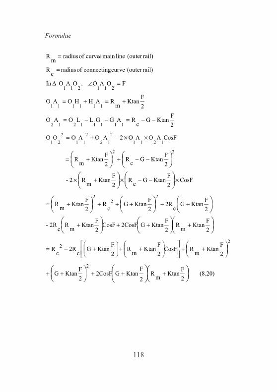
118

Formulae

(8.20) 2F

KtanmR2

FKtanG2CosF

2F

KtanG

2F

KtanmRCosF2F

KtanmR2F

KtanGc

2Rc

R

2F

KtanmR2F

KtanG2CosFCosF2F

KtanmRc

2R

2F

KtanGc

2R2F

KtanGc

R2F

KtanmR

CosF2F

KtanGcR2F

KtanmR2

2F

KtanGcR2F

KtanmR

CosFAOAO2AOAOOO

2F

KtanGc

RAGGLLOAO

2F

Ktanm

RAHHOAO

FOAOOAO ΔIn

rail)(outer curve connecting of radius c

R

rail)(outer linemain curve of radius m

R

2

22

22

2

22

12112

122

112

21

11111212

111111

211 ,

211

d

-

-

⎟⎠⎞

⎜⎝⎛⎟⎠⎞

⎜⎝⎛

⎟⎠⎞

⎜⎝⎛

⎟⎠⎞

⎜⎝⎛

⎥⎦⎤

⎢⎣⎡

⎟⎠⎞

⎜⎝⎛⎟⎠⎞

⎜⎝⎛

⎟⎠⎞

⎜⎝⎛

⎟⎠⎞

⎜⎝⎛

⎟⎠⎞

⎜⎝⎛

⎟⎠⎞

⎜⎝⎛

⎟⎠⎞

⎜⎝⎛

⎟⎠⎞

⎜⎝⎛

⎟⎠⎞

⎜⎝⎛

⎟⎠⎞

⎜⎝⎛

+++++

++⎟⎟⎠

⎞⎜⎜⎝

⎛++⎟⎟

⎠

⎞⎜⎜⎝

⎛+−=

++++

+−++++=

×−−×+×

−−++=

××−+=

−−=−−=

+=+=

=

=

=

∠

119

(8.21) 2

FKtan

2F

Ktan-G-DmR2CosF

2F

Ktan2F

Ktan-G-DmR

2F

Ktan-CosF2F

Ktan-G-DmRc

2Rc

R

2

FKtan

2F

Ktan-G-DmR2CosF2F

Ktan-G-DmRc

2R

2F

Ktan-G-DmR2F

Ktan2

FKtan

c2R

cR

CosF2F

KtancR2F

Ktan-G-DmR2-

2F

KtancR2F

Ktan-G-DmR

CosFAOAO2AOAOOO

2F

Ktanc

R AO

2F

Ktan-G-Dm

RAGGL-LOAO

FOAOOAO ΔIn

22

2

222

22

22212

222

212

21

22

2222

21

21

221 ,

221

⎟⎠⎞

⎜⎝⎛

⎟⎠⎞

⎜⎝⎛

⎟⎠⎞

⎜⎝⎛

⎥⎦⎤

⎢⎣⎡

⎟⎠⎞

⎜⎝⎛

⎟⎠⎞

⎜⎝⎛

⎟⎠⎞

⎜⎝⎛

⎟⎠⎞

⎜⎝⎛

⎟⎠⎞

⎜⎝⎛⎟⎠⎞

⎜⎝⎛

⎟⎠⎞

⎜⎝⎛

⎟⎠⎞

⎜⎝⎛

+

+++

⎟⎟⎠

⎞⎜⎜⎝

⎛+−=

+−+−

++++=

++

+++=

×××++=

+=

+=−=

=

−

∠

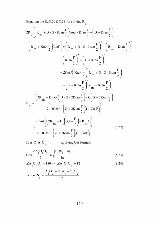
120

( )

( )

2

OOAOOAS where

(8.24)FOOA (180OOA

(8.23)bc

a)(SS

2

OOACos

formula Cos applyingOAO ΔIn

(8.22)

CosF12F

2KtanG-DCosF2

GmR2F

KtanDm2R2CosF

-

CosF12F

2KtanG-DCosF2

2F

2KtanGG2F

2Ktan-G-DG-Dm2R

cR

2

FKtan

mR

2

FKtanG

2

FKtan-G-D

mR

2

FKtanCosF

2

FKtanG

2

FKtan

2

FKtan

mR

2F

Ktan-G-DmRCosF2F

KtanmR

2

FKtanG

2F

Ktan-CosF2F

Ktan-G-DmRc

2R

cR solvingfor 8.21 & 8.20 Eq theEquating

2111211

211121

11211

,211

22

22

)

2

++=

∠−=∠

−=

∠

+⎟⎟⎠

⎞⎜⎜⎝

⎛+

⎥⎥⎦

⎤

⎢⎢⎣

⎡+⎟

⎠⎞⎜

⎝⎛ +

+⎟⎟⎠

⎞⎜⎜⎝

⎛+

⎟⎟⎠

⎞⎜⎜⎝

⎛+−⎟⎟

⎠

⎞⎜⎜⎝

⎛⎟⎠⎞⎜

⎝⎛ +

=

+++

+

+−

+−+=⎟⎟⎠

⎞⎜⎜⎝

⎛+−

+−⎟⎟⎠

⎞⎜⎜⎝

⎛+

+

⎥⎦⎤

⎢⎣⎡

⎟⎠⎞

⎜⎝⎛

⎥⎦⎤

⎢⎣⎡

⎟⎠⎞

⎜⎝⎛⎟⎠⎞

⎜⎝⎛

⎟⎠⎞

⎜⎝⎛⎟⎠⎞

⎜⎝⎛−

⎟⎠⎞

⎜⎝⎛

⎟⎠⎞

⎜⎝⎛+

⎟⎠⎞

⎜⎝⎛

⎟⎠⎞

⎜⎝⎛

⎥⎦⎤

⎟⎠⎞

⎜⎝⎛

⎢⎣⎡

121

Degreesin is φ'' where180

φcRS

curveinner to

curveouter thefrom K'' of valuesof projection theis mR

KD

Degreesin is '' where

(8.27)mR

KD2K

180

θmRX

OOAOOAφ

OOAOOAθ

2

OOAOOAS where

(8.26)F)OOA (-180 OOA

(8.25)bc

a)(SS

2

OOACos

formula, Cos applying ,OAO ΔIn

π

π

θ

121122

212211

2121222

212122

22212

221

××=

−+=

∠−∠=∴

∠−∠=∴

++=

+∠=∠

−=

∠

⎟⎟⎠

⎞⎜⎜⎝

⎛

Note:

When we introduce straight crossing on curves, we introduce kinks onthe junction of the crossings on either end. The curve is allowed tomaintain same curve outside. Similar kinks will appear on the ends ofcrossings on the connecting track. In some countries the main linecurves are realigned after introducing crossings. This type of layoutsare only suitable when the main line curve is fairly easy. It is found thatif thee calculations are being done by assuming them as that forcrossover connection between two straight parallel tracks, thedifference between them is negligible. If we calculate for ‘X’ assumingthem as two straight parallel track at a track centre of ‘D’, then,

2

FGCotDCotFX −=

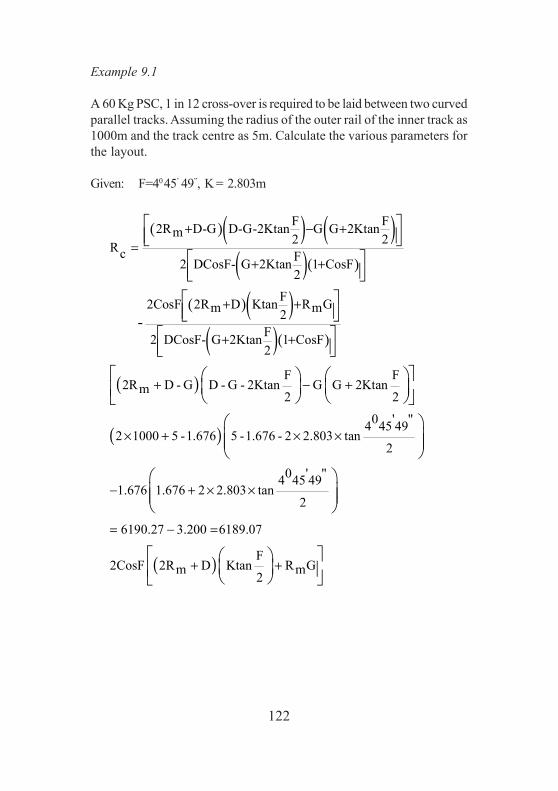
122

Example 9.1

A 60 Kg PSC, 1 in 12 cross-over is required to be laid between two curvedparallel tracks. Assuming the radius of the outer rail of the inner track as1000m and the track centre as 5m. Calculate the various parameters forthe layout.

Given: F=40 45’ 49”, K = 2.803m

( )( ) ( )( )( )

( )( )( )( )

( )

( )

F F2R D-G D-G-2Ktan G G 2Ktanm 2 2Rc F2 DCosF- G 2Ktan 1 CosF2

F2CosF 2R D Ktan R Gm m2F2 DCosF- G 2Ktan 1 CosF2

F F2R D - G D - G - 2Ktan G G 2Ktanm 2 2

2 1000 5 -1.676 5 -1.676 - 2 2

-

+ − +=

+ +

+ +

+ +

+ − +

× + ×

⎡ ⎤⎢ ⎥⎣ ⎦

⎡ ⎤⎢ ⎥⎣ ⎦⎡ ⎤⎢ ⎥⎣ ⎦

⎡ ⎤⎢ ⎥⎣ ⎦

⎡ ⎤⎛ ⎞ ⎛ ⎞⎜ ⎟ ⎜ ⎟⎢ ⎥⎝ ⎠ ⎝ ⎠⎣ ⎦

( )

0 ' "4 45 49.803 tan

2

0 ' "4 45 491.676 1.676 2 2.803 tan

2

6190.27 3.200 6189.07

F2CosF 2R D Ktan R Gm m2

×

− + × ×

= − =

+ +

⎛ ⎞⎜ ⎟⎜ ⎟⎝ ⎠

⎛ ⎞⎜ ⎟⎜ ⎟⎝ ⎠

⎡ ⎤⎛ ⎞⎜ ⎟⎢ ⎥⎝ ⎠⎣ ⎦

123

( )

( )

( )

0 ' "4 45 490 ' "2 Cos4 45 49 2 1000 5 2.803 tan 1000 1.6762

3805.97

F2 DCosF - G 2Ktan 1 CosF

2

0 ' "4 45 490 ' " 0 ' "2 5 Cos4 45 49 - 1.676 2 2.803 tan 1 Cos4 45 492

2.3416189.07 3805.

Rc

× × + × + ×

=

+ +

× + × × +

=−

=

⎡ ⎤⎛ ⎞⎢ ⎥⎜ ⎟⎜ ⎟⎢ ⎥⎝ ⎠⎣ ⎦

⎡ ⎤⎛ ⎞⎜ ⎟⎢ ⎥⎝ ⎠⎣ ⎦

⎡ ⎤⎛ ⎞⎢ ⎥⎜ ⎟⎜ ⎟⎢ ⎥⎝ ⎠⎣ ⎦

( ) ( )

1 1

2 1

1 2

971017.98m

2.341for solving 'θ'

0 ' "F 4 45 49O A R Ktan 1000 2.803 tan 1000.12mm 2 2

0 ' "F 4 45 49O A R G Ktan 1017.98 1.676 2.803 tanc 2 2 1016.18m

2 2O O 1000.12 1016.18 2 1000.12 1016.18 Co

=

= + = + × =

= − − = − − ×

=

= + − × × ×

1

1 1 2

1 1 20 -

0 ' "s4 45 49

85.312m1000.12 1016.18 85.31

S 1050.80m2

A O O 1050.80(1050.8 1016.18)Cos2 1000.12 85.13

' "A O O 98 21 46.01−

=+ +

= =

∠ −=×

∴∠ =

124

1 2

2 2

2

2 1 2

0

0

FO A R D G Ktanm 2

' "4 45 49 1000 5 1.676 2.803 tan 1003.20

2' "F 4 45 49

O A R Ktan 1017.98 2.803 tan 1018.10c 2 21003.2 1018.10 85.31

S 1053.302

A O O 1053.3(1053.3 1018.10)Cos2 1003.20 85.13

= + − −

= + − − × =

= + = + × =

+ += =

∠ −=×

∴ 2 1 2

1 1 2 2 1 2

0 3

0 0- 21 46

0

0

' " A O O 97 40 1.8

' " ' "θ A O O A O O 98 .0 97 40 31.8

' "0 4114.8R θ KDmX 2K 180 Rm

' "1000 0 4114.8 2.803 52 2.803 17.60m

180 1000If we solve the above problem as that for crossover conne

π

π

∠ =

= ∠ − ∠ = −

=

= + −

× × ×= + × − =

( )

ction

between straight parallel tracks, then0 ' "F 4 45 49

X DCotF - GCot 5 12 1.676 Cot 19.71m2 2

The difference between the two values is 17.60-19.71 2.11m

= = × − × =

=

125

Chapter 10

Software on Layout Calculations

10.1 Introduction

In their day to day work P. way officials have to deal with complicatedyard layouts. The maintainability and riding quality over a turnout dependslargely on how accurately it is laid and maintained. Kinks in points andcrossings can be avoided if adequate care is taken at the time of layingitself.

For ensuring correct laying it is essential that necessary calculations arecorrectly done before layouts are laid in the field. These calculations areintricate in nature and require considerable efforts on the part of P. Wayofficials .Due to their remaining busy in routine works on many occasionsthis item of work does not get the attention it deserves.

10.2 Layouts

While the insertion of crossover, diamonds in existing layouts, yardremodelling etc. are being taken up, errors in calculations may result in:

• Incorrect laying (i.e. incorrect TNC distances) – Results inbad running and in extreme cases unsafe conditions mayoccur on defective/bad layouts.

• Long crossovers at angle ‘F’ being laid even though spacecould be saved by having curves in between two turnouts.

• During doubling/gauge conversion projects new layouts arebeing inserted forcible resulting into undesirable curvatureswhich give bad running and are potential locations needingfrequent attention.

• It is suggested that even while replacing an old layout anopportunity be taken to correct all known defective layouts.

126

The book on “Layout Calculations” gives all the formulae and samplecalculations and is of great help in ensuring correct laying of crossoversand other connections. For assisting the field engineers, a software hasbeen developed in Visual Basic for all the cases presented in the book on“Layout Calculation”. The salient features of the Software are:

• Highly interactive• No need to refer to any book• All data on standard dimensions stored in subroutines• Crossings can be fixed straight away based on these

calculations

10.3 Scope

The Software covers the following:

Connections between

• Diverging Tracks• Straight Parallel Tracks• Curved Parallel tracks• Curved and straight Tracks

Cross-overs between

• Straight Parallel Tracks• Non Parallel Straight Tracks• Curved Parallel tracks• Sanded Dead End and Main Line• Double Junction

The Software generally follows the pattern as given in the book on“Layout Calculations”.

While running the Software for a particular case, the user has to give thedata on section, Details of crossing from a drop down menu, trackcenters, Radius of connecting curve etc and the results are obtainedinstantaneously.

127

10.4 Instructions for Using the Software

Installation

For installing the Software insert the CD in your CD drive. Go to “Mycomputer” select the drive containing the CD; locate the “set up” filefrom the “Layout” folder or subfolder and double click the setup icon.The Software will be installed instantaneously on your computer and willbe available in your “start” menu.

Alternately if you do not wish to install the Software go to start menuselect the ”Run” command and on browsing locate the file“Layout_Calculations.exe” in your CD and Click “OK” and the Softwarewill get loaded.

10.5 Illustration

As soon as the Software is loaded, the following screen is visible:

You can select either “Connections” or “Crossovers” from amongst thetwo option buttons. “Connections” or “Crossovers” as referred earlier.

Since running the Software is similar in almost all cases of “Connections”and “Crossovers’,only two cases of each type will be described forillustration.

128

Let us first take “Connections”. After choosing the “Connections” optionbutton and clicking “Proceed” Button next to screen opens as givenbelow giving list of options under “Connections”.

Let us select “Connections to straight parallel track” and click “Proceed”Button .It opens the next Screen which gives a sketch and text boxes fordata entry.

Certain features of the Software are common to all the cases and are listedbelow:

• Selecting the appropriate Gauge option opens a drop menu forstandard turnout dimensions on BG or MG as the case may be.The labels of the items needing data entry have been shadedwhite. Other text boxes are locked and will not accept any data.They will only display results.

• Units of dimensions have to be in mm except where specificallymentioned.

• Please ensure that data in all text boxes requiring data entry arecorrectly entered and the type of turnout is selected from thedrop down menu before clicking “Compute” Button else youwill get run time errors.

129

• For non Standard turnouts the red label is required to be clickedas indicated on the screen and it opens text boxes for givingdata on turnouts viz. description, turnout number (e.g. 12 incase of 1 in 12 turnouts) and centre line dimensions A,M,K etc.

• The most ideal type of suggested output is to take a print ofthe form displaying the results by clicking “Print” Button.Alternately textural output on a file is also possible. For thispurpose the Button “Copy results in a file” is to be clickedwhich will open an input box to give the file name for output.Please be sure to enter the complete file name with drive nameand folder where you want the output. The output file socreated can be easily opened in any text editor such as Wordpad.

• The Software also gives warnings by way of displayingmessage boxes – when results are unacceptable such asresulting curvatures being sharp and beyond permissible limitsspecified of Schedule of dimensions.

On getting the Screen as mentioned above, the values have to beentered. We have to select the appropriate turnout from drop down menuand on clicking compute button results in the screen to appear as under:

130

The second case for demonstration in “Connections” is taken as“Connections between Curved and straight track”. On Clicking the“Proceed” Button it opens the appropriate screen which has separateframes for Gauge selection and for whether the intersection on the insideor outside of the curve. After you select appropriate Gauge and thentype of intersection would display appropriate sketch and after completedata entry and clicking “Compute” Button would give the results asshown below:

Next we take the Cases of “Cross-overs”. On selecting Crossovers fromthe first screen as described in Para 5.3 and clicking “ Proceed Buttontakes us to the screen showing the choices under “ Crossovers”

131

Let us first take the case “Cross-overs at large spacing with no straight inbetween” On selecting Gauge, appropriate Turnout from the drop downmenu and entering all the data we get following screen after clickingCompute Button.

If the same case is solved treating it as a case for non standard turnoutthen the text of the drop down menu is to be changed as “other type” inlower case and it opens the new text boxes for entering the data for theturnouts. On entering a sample data and clicking the “ compute” buttongives the following results.

The above feature is available in all the cases.

132

We take the next case of Crossovers between inclined tracks. The finalresults after entering data etc is as below:

10.6 Conclusions

It is considered that the Software explained above would be ofconsiderable help to the field Engineers in improving the running qualityover turnouts and ensuring safety by way of correct laying.

133

L TSL SL d w F R

1 in 8 ½ 60 kg C, FH. 18424 7872 7135 182.5 880 60-42’-35” 40-35’-0” 2314401 in 8 ½ 52 kg S, LH 20730 4950 4725 136 864 60-42’ 35” 10-34’-27” 2223601 in 8 ½ 52 kg C, FH 18395 6835 6400 182.5 864 60-42’ 35” 00-47’-27” 2323201 in 8 ½ 90R S, LH 20730 4950 4725 136 864 60-42’ 35” 10-34’-27” 2223601 in 8 ½ 90R C, FH 18395 6835 6400 182.5 864 60-42’-35” 00-47’-27” 2323201 in 12 60 kg C, FH 25831 11156 10125 175 1877 40-45’-49” 00-20’-0” 4413601 in 12 52 kg C, FH 29200 6724 6400 133 1232 40-45’-49” 10-0’44” 4421201 in 12 52 kg S, FH 27870 8478 10125 133 1232 40-45’-49” 00-27’-35” 4581201 in 12 90 R C, FH 29200 6724 6400 133 1232 40-45’-49” 10-8’-0” 4421201 in 12 90 R S, FH 27870 8487 7730 133 1232 40-45’-49” 00-17’-11” 4581201 in 16 52 kg C, FH 37170 10594 6500 153 1377 30-34’-35” 00-24’-27” 8242251 in 16(HS) 52 kg C, FH 37565 12320 7730 133 1377 30-34’-35” 00-24’-27” 8164801 in 16) 90R C, FH 37170 10594 9750 133 1377 30-34’-35” 00-46’-59” 8242251 in 20 90R C, FH 46210 11194 11150 133 1377 20-51’-45” 00-46’-59” 1303810

1 in 8 ½ 60 kg C, FH 18395 6839 6400 182.5 1225 60-42’-35” 00-46’-59” 2322601 in 8 ½ 52 kg C, FH 18395 6839 6400 182.5 1225 60-42’-35” 00-46’-59 2322601 in 12 60 kg C, FH 25831 10125 10125 175 1877 40-45’-49” 00-20’-0” 4413601 in 12 60 kg C, FH 25831 10125 10125 175 1877 40-45’-49” 0 0-20’-0” 4413601 in 16 60 kg C, FH 35720 11200 11200 145 2526 30-34’-35” 00-20’-0” 7849931 in 20 60 kg C, FH 46027 12460 12460 133 1877 20-51’-45” 00-20’-0” 1283100

1 in 8 ½ 90R C, FH 9515 6206 5500 169 915 60-42’-35” 00-29’-13” 1302101 in 8 ½ 75R S, LH 11560 4320 4115 120 915 60-42’-35” 10-35’-30” 1196101 in 8 ½ 75R C, FH 9515 6206 5500 169 915 60-42’-35” 00-29’-14” 1302101 in 8 ½ 60R S, LH 11560 4320 4115 120 915 60-42’-35” 00-24’-27” 1196101 in 8 ½ 60R C, FH 9515 6206 5500 169 915 60-42’-35” 10-9’-38” 1302101 in 12 90R Partly C, FH 14678 7974 7130 130 1220 40-45’-49” 00-24’-27” 2583001 in 12 75R S, FH 16323 5777 5485 117 1220 40-45’-49” 10-9’-38” 2406001 in 12 75R Partly C, FH 15108 7544 6700 117 1220 40-45’-49” 00-24’-27” 2583001 in 12 60R S, FH 16323 5777 5485 117 1220 40-45’-49” 10-9’-38” 2406001 in 12 60R Partly C, FH 15108 7544 6700 117 1220 40-45’-49” 00-24’-27” 2583001 in 16 60R C, FH 20060 8264 7420 117 1378 30-34’-35” 00-24’-27” 46240

1 in 8 1/2 HTC 52 Kg C, FH 9515 6206 5500 169 1047 60-42'-35" 00-29'14" 1302051 in 12 CMS 52 Kg Partly C, FH 14678 7974 7130 130 1405 40-45'-49" 00-24'-27" 258310

1 in 8 ½ 60R S, LH 8280 4320 4115 120 915 60-42’-35” 10-35’-30” 828001 in 12 60R S, LH 11723 5777 5485 117 1220 40-45’-49” 10-9’-389” 167340Note: C Curved

FH Fixed HeelLH Loose HeelCMS Cast Manganese Steel CrossingHTC Heat Treated CrossingHS High Speed

Narrow Gauge

Metre Gauge on PSC Sleepers

Broad Gauge (1673 mm) on PSC Sleepers

TABLE OF DETAILED DIMENSIONS

Metre Gauge

Dimensions (mm)

Broad Gauge

Crossing No Section Typeβ

134

A B C M K52 KG BG 1 IN 8 1/2 S, LH 12000 16274 840 14295 1979 RDSO T/28552 KG BG 1 IN 8 1/2 C, FH 12000 16274 1500 14295 1979 RDSO/T-28690 R BG 1 IN 8 1/2 S, LH 12000 16260 840 14295 1965 RDSO/T-36090 R BG 1 IN 8 1/2 C, FH 12000 16260 1500 14295 1965 RDSO/T-30752 KG BG 1 IN 12 S, FH 16953 22706 1500 20147 2559 RDSO/T-3252 KG BG 1 IN 12 C, FH 16953 22706 1500 20147 2559 RDSO/T-18490 R BG 1 IN 12 S, FH 16953 22687 1500 20147 2540 RDSO/T-18490 R BG 1 IN 12 C, FH 16953 22687 1500 20147 2540 RDSO/T-3152 KG BG 1 IN 16 C,FH 20922 30750 844 26842 3908 RDSO/T-13552 KG BG 1 IN 16 (HS) C,FH 22693 30750 850 26842 3908 RDSO/T-23190 R BG 1 IN 16 C,FH 20922 30750 844 26842 3882 RDSO/T-6790 R BG 1 IN 20 C,FH 24664 38118 844 33540 4578 RDSO/T-98

A B C M K52 KG BG 1 IN 8 1/2 S, LH 12000 17418 840 14295 3123 TA-20122,

TA-2080452 KG BG 1 IN 8 1/2 C, FH 12000 17418 1500 14295 3123 TA-20196,

TA-2083590R BG 1 IN 8 1/2 S, LH 12000 17404 840 14295 3109 TA20110,

TA-20198,etc90R BG 1 IN 8 1/2 C, FH 12000 17404 1500 14295 3109 TA-20148,

TA-2082252 KG BG 1 IN 12 S, FH 16953 23981 1500 14295 3834 TA-5268(M),

TA-20222, TA-20801

52 KG BG 1 IN 12 C, FH 16953 23981 1500 20147 3834 TA-20171, TA-20831

90R BG 1 IN 12 S, FH 16953 23962 1500 20147 3815 TA-5044(M), TA-20184, etc

90 R BG 1 IN 12 C, FH 16953 23962 1500 20147 3815 TA-20125, TA-20839

52 KG BG 1 IN 16 C, FH 20922 31447 844 20147 4605 TA-20141, TA-20828

52 KG BG 1 IN 16 (HS) C, FH 22693 31447 850 26842 4605 RDST/T-40390 R BG 1 IN 16 C, FH 20922 31421 844 26842 4579 TA-20138,

TA-2081390 R BG 1 IN 20 C, FH 24664 39470 844 26842 5930 TA-20122,

TA-2080460 KG BG (PSC)1 IN 8 1/2 C, FH 12025 16486 1500 14270 2216 RT-486552 KG BG (PSC)1 IN 8 1/2 C, FH 12025 16486 1500 14270 2216 RT-486560 KG BG (PSC)1 IN 12 C, FH 16989 22912 1141 20111 2803 RT-421852 KG BG (PSC)1 IN 12 C, FH 16989 22914 1141 20111 2801 RT-421860 KG BG(PSC) 1 IN 16 C,FH 20970 30558 844 26794 3764 RDSO/T-569160 KG BG(PSC) I IN 20 C, FH 25850 38031 844 33480 4550 RDSO/T-5858

Assembly Drg No

Section Gauge crossing No Type

TABLE OF DETAILED DIMENSIONS

CENTRE LINE LAYING (FOR BG WITH CMS CROSSING)

Section Gauge Crossing No Type Dimensions (mm) Assembly Drg No

CENTRE LINE LAYING ( FOR BG WITH ORDINARY CROSSING)

Dimensions (mm)

135

Assembly Drg

No

A B C M K RDSO/T

1 in 8.5 75R S, LH 7986 10376 840 8529 1847 393

1 in 8.5 75R C,FH 7986 10376 1500 8529 1847 386

1 in 8.5 60R S, LH 7986 10360 840 8529 1831 379

1 in 8.5 60R C, FH 7986 10360 1500 8529 1831 372

1 IN 12 75R S, FH 11287 14321 1500 12021 2300 394

1 IN 12 75R PARTLY C, FH 11287 14321 1500 12021 2300 401

1 IN 12 60R S, FH 11287 14296 1500 12021 2275 367

1 IN 12 60R PARTLY C, FH 11287 14296 1500 12021 2275 423

1 IN 16 75R C, FH 12309 19054 844 16015 3039 189

1 IN 12 (PSC) 52KG Partly C, FH 11287 14489 1500 12021 2468 T-6450

1 IN 8.5 (PSC) 52 KG C, FH 7986 11932 1500 8529 3403 T-6327

1 IN 8.5 90R C, FH 7981 11638 1500 8530 3108 TA-20497

1 IN 8.5 75R S, LH 7986 11632 840 8529 3103 TA-20404,

TA-21004

1 IN 8.5 75R C, FH 7986 11632 1500 8529 3103 TA-20451,

TA-21019

1 IN 8.5 60R S, LH 7986 11615 840 8529 2086 TA-204007,

TA-20460

1 IN 8.5 60R C, FH 7986 11615 1500 8529 2086 TA-20463,

TA-21007

1 IN 12 90R Partly C, FH 1286 15176 1500 12021 3155 TA-20416

1 IN 12 75R S, FH 11287 15166 1500 12021 3145 TA-20466

1 IN 12 75R Partly C, FH 11287 15166 1500 12021 3145 TA-20401,

TA-21001

1 IN 12 60R S, FH 11287 15143 1500 12021 3122 TA-20464,

TA-21016

1 IN 12 60R Partly C, FH 11287 15143 1500 12021 3122 TA-21410,

TA21410,

TA-21010

1 IN 16 60R C, FH 12309 19635 844 16015 3680 TA-20466

TA-20413,

TA-21013

1 in 8.5 60R S, L H 6736 9585 840 6499 3086 TA-20604

1 in 12 60R S, FH 9548 12282 1500 9160 3122 TA-20601

Metre Gauge ( with CMS crossing)

Metre Gauge ( with Ordinary crossing)

Narrow Gauge (with Ordinary crossing)

Meter Gauge (with Heat Treated crossing)

TABLE OF DETAILED DIMENSIONS

CENTRE LINE LAYING (FOR METRE GAUGE)

Dimensions (mm)Crossing No Section Type

80