Singularity theorems in Schwarzschild spacetimes

Servando V. Serdio1, Hernando Quevedo1,2,3∗

1Instituto de Ciencias Nucleares, Universidad Nacional Autonoma de Mexico,

AP 70543, Mexico, DF 04510, Mexico

2Dipartimento di Fisica and ICRANet,

Universita di Roma “La Sapienza”, I-00185 Roma, Italy

3Institute of Experimental and Theoretical Physics,

Al-Farabi Kazakh National University, Almaty, Kazakhstan

(Dated: January 31, 2020)

Abstract

We present a review of the two prominent singularity theorems due to Penrose and Hawking,

as well as their physical interpretation. Their usage is discussed in detail for the Schwarzschild

spacetime with positive and negative mass. First, we present a detailed mathematical proof to

formally guarantee the existence of a singularity of geodesic incompleteness for the case of positive

mass. Second, we discuss the applicability of the mathematical tools used by the theorems in the

negative mass case. The physical implications of the validity or inconsistency of the hypotheses

of such theorems on the latter case, are also exhibited. As far as this analysis is concerned, some

clues are produced regarding future research that could result in general properties for naked

singularities.

Keywords: Singularities, singularity theorems, Penrose, Hawking-Penrose, Schwarzschild

spacetime, global hyperbolicity, generic condition, trapped points, trapped surfaces

PACS numbers: 05.70.Ce; 05.70.Fh; 04.70.-s; 04.20.-q

∗Electronic address: svserdio@correo.nucleares.unam.mx,quevedo@nucleares.unam.mx

1

arX

iv:2

001.

1137

6v1

[gr

-qc]

30

Jan

2020

I. INTRODUCTION

The theory of singularities in general relativity represents an enlightening theoretical

development that, despite being around for about 50 years by now, keeps captivating the

attention of beginners and specialists. Nobody (even without any training in physics) should

doubt its profound significance and implications to our understanding of the Universe. The

discovery of singularities, as an inevitable (and generic) consequence of one of the most

successful physical theories in history, rocked our minds to their core. The experimental

astronomical observations to date, together with a vastly tested and many times corrobo-

rated theory like general relativity, suggest that: (a) a long (but finite) time ago, the stuff

that constitute everything around us might have suddenly started to exists under a set of

rules (e.g. the theory itself) that seem to be oblivious of that initial event, and (b) a similar

(but time reversed) phenomenon seems to take place when enough energy-matter is brought

together inside a bounded spatial region. Such a content of matter (or at least part of it)

would collapse on itself until it reaches such an extreme state that its existence comes to an

end (i.e. it ceases to exist within the framework of the theory, and cannot be described any

longer by means of it)

Whether or not one is willing to accept a sudden “creation” or an inevitable final fate as

the ultimate consequences of the singularity theorems, they surely state without a doubt a set

of circumstances under which one cannot rely anymore on the theory to make predictions.

As if general relativity where not astounding enough, certain cases in which its validity

cannot be assumed any longer are plainly exposed by the theory itself via the theorems in

question.

With such profound implications, and as it should be the case, a huge variety of results

have been motivated by the singularity theorems after the first one of their kind (due to Pen-

rose) was published in 1965 [1]. An extensive and illustrative summary of the antecedents,

concepts and consequences of that particular theorem can be found in [2]. Specifically

speaking, the novelty of such theorem (and the other classical one that succeeded it, due

to Hawking and Penrose [3]) resides in its use of an original concept called a closed trapped

surface (that captures the idea of an inevitable and instantaneous total confinement scenario

for an enclosed energy-matter distribution) which, together with other geometric properties

of a given spacetime (like an “energy” condition and some sort of global causality), tends to

2

favour the formation of geodesic incompleteness within such spacetime (being this the very

same concept representing the aforementioned notion of sudden creation/disappearance of

particles, also presented for the first time by Penrose).

It is not an overstatement to say that all the research that have been motivated by the

first theorems is vast and can easily lead to bewilderment. Despite the existence of works

like [2, 4, 5] that can be used as a first guide to the nowadays world of singularities, as soon

as one steps outside of them one immediately has to face a menagerie of results that (in

one way or another) were inspired by the three notions/concepts previously mentioned. In

order to briefly give some particular examples related to the main conclusions derived from

the following sections (that in no way constitute an exhaustive list, but that are intended to

broaden in here the outlook of their corresponding subjects), three categories (most likely

intertwined) can be made.

First, the concept of a trapped surface has been a very prolific one as it can be generalized

in several ways thanks to its possible characterization via the mean curvature vector field

[2]. By virtue of this vector field, in particular, closed trapped submanifolds of arbitrary

co-dimension can be defined in order to generalize the Hawking-Penrose theorem [6]. In a

similar manner, the Penrose theorem can be generalized to include surfaces to some extent

“less trapped” (like marginally outer trapped surfaces, for example), and to approach the

possible formation of singularities from an initial data set (i.e. the so called initial data

singularity theorems) [7]. Additionally, and with respect to more recent incursions of the

trapped surface concept into the realm of black hole physics, the notion of the smallest

trapped region in a spacetime can be used to define the boundary of black holes that do not

necessarily belong to stationary spacetimes [8]. By virtue of the present work, the notion

of a trapped surface could even be used to hint the existence of (curvature) singularities,

despite those submanifolds not representing total confinement.

Second, the earliest attempts to address the natural question of whether or not additional

information about a singularity of geodesic incompleteness could be extracted from the

theory (apart from their mere existence), were promptly made after the first singularity

theorems were proven. From theorems stating conditions under which a spacetime could be

extended to include a singularity (in a smoothly enough manner) [9–12], to theorems and

results categorizing singularities by the way in which certain scalar magnitudes diverge when

traversing the curves leading to them [13–16], the issue has shown to be a complicated one

3

to resolve (most likely because, in a strict sense, singularities are not part of the spacetime

“possessing” them and cannot be analyzed like any other geometric object). As far as the

present work is concerned, some restrictions can be imposed on the rate at which the stress

tidal tensor (with respect to a parallelly propagated orthonormal/pseudo-orthonormal basis)

grows towards a singularity of geodesic incompleteness [16]. As exposed in the following

analysis of the Schwarzschild spacetime, not every component of such tensor is restrained

to diverge with the rate in question towards singularities in null incomplete geodesics. As

it turns out, the use of such decomposition for the tidal stress tensor might even provide

information regarding the repulsive or attractive nature of a singularity. This feature could

be used to shed some light into the soundness of new ideas intended to precisely define

repulsive gravitational effects [17].

Third, the profound conceptual (and philosophical) repercussions of the theorems have

always been largely based on the seeming physical feasibility of their hypotheses. Never-

theless, with only local experimental evidence at our disposal, it is only natural to explore

the possibility of weakening or even changing/improving some of those assumptions. Ex-

cellent expositions of the ideas behind some efforts on the matter, and the results obtained

concerning the so called rigidity theorems, can be found in [18–20]. Although important

generalizations of the classical theorems have been accomplished in relation to, for example,

the weakening of requirements like smoothness or global causality [21, 22], it also has being

possible to relax the boundary/initial condition of the theorems (appearing in the form of

trapped submanifolds). As mentioned earlier, the use of the mean curvature vector field

allows for “lesser trapped” scenarios to be considered, and singularity theorems have been

shown to hold for spacetimes possessing marginally and marginally outer trapped surfaces

[23]. One of the main results of the following exposition consists in showing an example

of another way in which a trapped surface (that is not closed nor it represents inevitable

confinement) could be used to hint the presence of singularities.

Finally, it goes without saying that the Schwarzschild spacetime has always played an

invaluable role in the development of the general theory of relativity and its experimental

corroboration. Since every introductory relativity book makes use of such solution to derive

classical tests of the theory, and to plainly show some illustrative effects, its significance is

beyond dispute. Regarding the impact of studies exploiting spherical symmetry to the theory

of singular spacetimes, it is worth to recall that from the very first theoretical indication

4

(to more recent ones) of the (possible) production of singularities by gravitational collapse,

an exterior vacuum Schwarzschild spacetime has always been matched to another collapsing

interior solution [24, 25]. Additionally, such level of symmetry has also been used, among

many other things, to understand the global properties of closed trapped surfaces [26], to

attempt to define the boundary of non-stationary black holes [8], and to rule out low classes

of extensions with which one could otherwise attach a singularity to its spacetime [27].

Within this context, the present article exploits once again the analytical manageability of

the Schwarzschild solution to exhibit specific geometrical properties that could hopefully

render new topics for singularity research.

The contents of the next exposition have the following structure. In section II, the

theorems of Penrose and Hawking-Penrose are presented, along with physically explanatory

interpretations for each one of their hypotheses. Section III contains a precise definition

of the innermost Schwarzschild vacuum spacetime with positive mass (i.e. the black hole

region of the full Schwarzschild solution, viewed as a manifold on its own), followed by a

detailed proof (split into several subsections) of the fulfilment by such spacetime of Penrose’s

theorem hypotheses. In section IV, the main differences between the cases of positive and

negative mass are pointed out in order to precisely define the corresponding spacetime

for the latter. In the form of several subsections, the fulfilment or infringement by this

second spacetime of the hypotheses of both theorems (associated with compact gravitational

sources), are analyzed. Special attention is given to the physical causes and/or implications

of the obtained results. Lastly, some concluding remarks are given in section V. Natural

units with G = c = 1 are used throughout this paper.

II. REVIEW OF TWO SINGULARITY THEOREMS

The two singularity theorems used in the following sections are due to Penrose and

Hawking [28] and nowadays can be regarded as classical. Despite them being well known

and understood by now, it seems hard to find in the literature a concise and intuitive way

of understanding the physical meaning of their hBecause of this, and taking into account

the fact that they can be found in a variety of references, here they will be simply stated

right away, followed only by their physical interpretation in the context of a particular

spacetime structure. For the sake of completeness, it should be reminded here that the

5

concept of a spacetime simply refers to the collection of all possible positions and times (i.e.

events) in a space, together with the capacity to measure temporal and spacial distances.

Moreover, it should also be kept in mind that in these theorems a spacetime always refers to

a 4-dimensional differential manifold without a boundary that is paracompact, connected,

Hausdorff, and which is equipped with a (sufficiently well behaved) Lorentzian metric.

Theorem II.1 (Penrose (1965)) Let (M, gαβ) be a spacetime for which the following con-

ditions are met: (1) It is connected. (2) It is globally hyperbolic with a non-compact Cauchy

surface. (3) At each one of its points the inequality Rαβkαkβ ≥ 0 is satisfied by every null

vector kµ. (4) It contains a closed trapped surface. Then (M, gαβ) contains at least one null

geodesic that is incomplete

Interpretation. Given a spacetime such that: (1) There do not exist isolated regions

within it. (2) By knowing the initial conditions in a spacelike unbounded hypersurface, it is

possible (in principle) to determine the complete physical state at every other event. (3) The

gravitational interaction felt by light waves due to an energy-matter distribution is always

attractive. (4) There exists a spacelike 2-surface, that closes on itself, for which the two

families of light rays departing orthogonally from it have instantaneously decreasing area

wavefronts [29]. Then there exists at least one light ray trajectory that cannot be extended,

and which ends up after a finite extent.

Theorem II.2 (Hawking-Penrose (1970)) Let (M, gαβ) be a spacetime for which the

following conditions are met: (1) For every causal vector vµ, the inequality Rαβvαvβ ≥

0 holds. (2) There do not exist closed timelike curves within M . (3) Every causal and

inextensible geodesic possesses a point at which its tangent vector kµ satisfies the (so called)

generic condition k[αRβ]γδ[µkν]kγkδ 6= 0. (4) There exists within M at least one of the

following subsets: (a) A compact and non-chronological set without an edge. (b) A closed

trapped surface. (c) A (trapped) point p such that the expansion of the family of null geodesics

emanating from it into the future (or past) always becomes negative along each one of these

geodesics. Then (M, gαβ) contains at least one causal geodesic that is incomplete.

Interpretation. Given a spacetime such that: (1) The gravitational interaction due to

an energy-matter distribution is always attractive for every collection of massive particles

and light waves. (2) No massive particle can have any influence on its own past. (3) Every

6

freely falling massive object experiments, at some moment in its history, tidal forces within

it. Also, along each light ray trajectory there exists a point such that, on accelerating a

massive object to near-light velocities in its direction, the tidal forces across its points become

a greater issue to overcome than its energy increase [18]. (4) There exists at least one of the

following sets: (a) A subset with no endpoints, despite being bounded, whose events cannot

influence their own past. (b) A closed trapped surface. (c) A point for which, along every

direction, the light waves emanating from it into the future always suffer a contraction at

some moment. Then there exists at least one freely falling massive particle trajectory, or a

light ray trajectory, that cannot be extended, and which ends up after a finite extent.

For more details on the physical interpretation of these singularity theorems, see [28, 30,

31].

III. SCHWARZSCHILD SPACETIME WITH POSITIVE MASS

It is a common practice in the literature to work out a formal proof of the previous

theorems and then simply state the validity of their hypothesis for a given spacetime. In the

case of the Schwarzschild solution, the Penrose diagram for its maximal (Kruskal-Szekeres)

extension can be used to visualize the applicability of theorem II.1 to it. Nevertheless, it

does not seem to exist so far a complete and detailed treatment addressing this fact. Even

if its confirmation is considered as straightforward and trivial as things can get, carrying its

details out definitely sheds some light into the key features that must be taken into account

when dealing with the theorems. It also opens up a window into the physical properties that

can be learned about a spacetime, via the mathematical tools used in the theorems. Because

of all of these reasons, special attention is given next to the definition of the spacetime itself.

A. The Schwarzschild spacetime

The spacetime to be considered (MSch, gαβ) consists of only the inner region (r < 2M) of

the (so called) exterior Schwarzschild solution. Specifically speaking, the manifold is given

by the set of points p ∈MSch ≡ O, for which a single chart {(O,Ψ)} is defined by means of

the map

p 7−−−→Ψ

(t(p), x(p), y(p), z(p)) ∈ R× Bo(2M),

7

FIG. 1: Three (well defined) different spherical open charts are required in order to completely

cover R3 \ {0}.

where M > 0 and Bo(2M) ≡ {(x, y, z) ∈ R3 | 0 < x2 + y2 + z2 < 4M2}. The metric gαβ is

introduced in the form (with x(1) ≡ x, x(2) ≡ y and x(3) ≡ z)

ds2 = −

(1− 2M√

x(i)x(j)δij

)dt2 + dx(i)dx(j)δ

ij

+2M√

x(i)x(j)δij − 2M

(δkmδlnx(k)x(l)dx(m)dx(n)

).

(1)

In order to relate this expression to the usual one in spherical coordinates (but in an

inconsistency free manner), three additional charts {(Oi,Ψi)}3i=1 must be taken into con-

sideration. The most common transformation between (flat) spherical and cartesian co-

ordinates are used to define these charts. The only difference between each chart being

the fact that the vertical direction is taken to coincide with a different cartesian coordi-

nate axis fixed in the background (Fig. 1). For example, the second one of these charts

corresponds to the case y = r sinϑ2 cosϕ2, z = r sinϑ2 sinϕ2 and x = r cosϑ2, with

(ϑ2, ϕ2, r) ∈ (0, π) × (0, 2π) × (0, 2M). It is then a matter of simple algebra to reduce

the previous line element to the form

ds2 =2M − r

rdt2 + r2

(dϑ2

i + sin2 ϑidϕ2i

)− r

2M − rdr2. (2)

Despite the fourth coordinate being timelike in this spacetime, it will remain being desig-

nated by the symbol r (i.e. the conventional spherical radial character) because of the way

it relates to the cartesian-like coordinates used in the first place. For this same reason, it

8

will also be referred to as the radial coordinate of the atlas in question. Furthermore, its

global nature (i.e. the fact that it takes a certain value for a point p ∈ MSch, regardless of

the neighbourhood Oi containing it) can be exploited to establish a temporal orientation

for the whole (MSch, gαβ). More specifically, every tangent vector Xµ whose components

(Xµ) = (X t, Xϑi , Xϕi , Xr) satisfy the condition Xr < 0, will be said to be future directed.

As can be anticipated from the way a spacetime is handled by the singularity theorems of

section II, the last construction comprises all of the basic structure required to corroborate

whether the hypotheses of the theorems are satisfied or not by (MSch, gαβ). The content

of the following subsections include some formal arguments regarding the applicability of

theorem II.1 to this spacetime.

B. Connectedness

Every Oi is clearly connected since its image, under the homeomorphism Ψi, is the set

R× (0, π)× (0, 2π)× (0, 2M). The fact that no two of the regions Oi are disjoint, guarantees

the connectedness of the whole MSch = ∪3i=1Oi [32].

C. Closeness and non-compactness of a hypersurface Sr0

By means of the following subsets (with 0 < r0 < 2M)

Sr0 ≡ {p ∈MSch|r(p) = r0}, Sr<r0 ≡ {p ∈MSch|0 < r(p) < r0}

and Sr>r0 ≡ {p ∈MSch|r0 < r(p) < 2M},(3)

a disjoint partition of the manifold MSch is made. Since Ψi(Sr0 ∩Oi) is closed in R× (0, π)×

(0, 2π) × (0, 2M), it also happens that Sr0 ∩ Oi is closed in Oi. If A represents the closure

of A ⊂MSch, it is clear that Sr0 ∩Oi = Sr0 ∩ Oi ∩Oi and Sr0 ∩Oi = Sr0 ∩ Oi ∩Oi. Because

of each Oi being an open subset of MSch, it is also the case that Sr0 ∩ Oi = Sr0 ∩ Oi [32].

From all the previous statements it is straightforward to obtain Sr0 = Sr0 .

On the other hand, Sr0 is clearly a Hausdorff topological space (with respect to its induced

topology) that can be covered by the collection of open sets Un ⊂MSch (n ∈ N), defined by

Ψ(Un ∩ O) ≡ (−n, n)× [Bo(r0 + ε) \ Bo(r0 − ε)] (with 0 < ε < r0). Since no finite subcover

for Sr0 can be extracted from {Un}n∈N, it follows that this hypersurface is not compact.

9

It is intuitively clear from the (by now standard) r−t diagram of the radial null geodesics,

that Sr0 is a good candidate for a Cauchy surface. The purpose of the following four

subsections is to formally corroborate that this is indeed the case.

D. Achronality of Sr0

Given a smooth timelike curve γ(τ), parameterized by its arc lenght τ , its tangent vector

components (t, ϑi, ϕi, r) (with a ≡ da/dτ) satisfy the relation

−1 =2M − r

rt2 + r2

(ϑ2i + sen2ϑiϕ

2i

)− r

2M − rr2.

Since r is a global coordinate for {(Oi,Ψi)}3i=1, the previous expression implies that r

never changes its sign nor it becomes equal to zero. In the case of having with γ a future

directed curve, the radial coordinate of its points will always be decreasing. This means

that for every such a curve, starting from p = γ(τ = 0) ∈ Sr0 into the future, r(τ) ≡ r[γ(τ)]

will be strictly greater than r(p) = r0 for τ > 0. The disconnected nature of the partition

MSch = Sr<r0 ∪ Sr0 ∪ Sr>r0 , guarantees then that I+ (Sr0) ⊂MSch \ Sr0 .

E. Future domain of dependence of Sr0: D+ (Sr0) = Sr<r0 ∪ Sr0

Consider a point p ∈ Sr<r0 and a smooth timelike curve γ that starts from p into the

past, that is past inextensible (within MSch) and which has been parameterized by its arc

lenght τ . Because of the temporal orientation that has been chosen, the following relation

will be satisfied along γ (within each Oi containing a segment of it)

r =

(2M − r

r

)1/2 [1 +

(2M − r

r

)t2 + r2

(ϑ2i + sen2ϑiϕ

2i

)]1/2

. (4)

Under the assumption of the parameter τ taking on every single value within [0,∞), it

is always possible to give a partition for this interval into segments [τi, τi+1), characterized

by (where O(i) ∈ {Oj}3j=1 for every i)

τ0 = 0,

γ(τ) ∈ O(i) ∀τ ∈ [τi, τi+1) ,

γ(τ) ∈ O(i+1) ∀τ ∈[τi+1, τ(i+1)+1

), with γ(τ∗) /∈ O(i) for some τ∗ ∈

[τi+1, τ(i+1)+1

).

(5)

10

By integrating (4) within each one of these intervals (and by taking into consideration the

continuity of r(τ)), the inequality 2M > r(τ) > (2M)−1/2∫ τ

0(2M − r)1/2 dτ ′ follows for ev-

ery τ ∈ [0,∞). This relation indicates the existence of the limits limτ→∞∫ τ

0(2M − r)1/2 dτ ′

and limτ→∞ (2M − r(τ))1/2 [33], which in turn guarantees that r(τ) −→ 2M when τ −→∞.

The immediate consequence of this statement is that γ ∩ Sr0 6= ∅, whenever the arc lenght

of such a curve is able to take on every single value within [0,∞).

In order to fully prove the desired identity for D+ (Sr0), it must also be considered having

γ ∩ Sr0 = ∅ for the curve in question. Nevertheless, the previous procedure forces τ to be

bounded from above for this case. If τM ≡ sup{τ} so that τ ∈ [0, τM), the increasing

feature of r(τ) implies the existence of rM ≡ sup{r(τ)} = limτ→τM r(τ) ≤ r0. By taking a

partition of [0, τM) identical to the one given in (5), a similar line of arguments leads now

to 2M > r(τ) > (2M)−1(2M − r0)∫ τ

0|t|dτ ′. Once again, this inequality guarantees that

tM ≡ limτ→τM t(τ) ∈ R [33].

On the other hand, it is also possible to give the following formulation for r

r =

(2M − r

2M

)1/2 [1 +

(2M − r

r

)t2 + r2 + r2(ϑ2

i + sen2ϑiϕ2i )

]1/2

.

The usefulness of this expression resides in the possibility to isolate from it the function

f(τ) ≡ {r2(τ)+r2(τ)[ϑ2i (τ)+sin2 ϑi(τ)ϕ2

i (τ)]}1/2. Because of the coordinate transformations

between the given atlases, it is obviously the case that this function has in fact a global nature

by admitting the formulation f(τ) = [x2(τ) + y2(τ) + z2(τ)]1/2. It is then a matter of simple

algebra to see that 2M > r(τ) > (2M)−1/2(2M − r0)1/2∫ τ

0f(τ ′)dτ ′. This again assures the

existence of xM ≡ limτ→τM x(τ), yM ≡ limτ→τM y(τ) and zM ≡ limτ→τM z(τ). Since it must

be the case that rM = (x2M + y2

M + z2M)1/2 (with 0 < r(p) ≤ rM ≤ r0 < 2M), the existence

of these three limits, and the one for t(τ), imply that Ψ(γ(τ)) = (t(τ), x(τ), y(τ), z(τ)) −→

(tM , xM , yM , zM) ∈ R× Bo(2M), when τ −→ τM . This obviously contradicts the inextensi-

bility of γ, and leads to the conclusion that γ ∩ Sr0 6= ∅.

The content of the previous procedure can be summarized as follows: every smooth

timelike curve that starts from Sr<r0 , and is past inextensible, intersects Sr0 . This entails

that Sr0 ∪ Sr<r0 ⊂ D+ (Sr0) [30].

On the other hand, the chosen temporal orientation also implies that γ′ ∩ Sr0 = ∅,

for every smooth timelike curve γ′ that starts from Sr>r0 and is past inextensible. By the

same reason as before, this last statement implies the inclusion Sr>r0 ⊂MSch\D+ (Sr0). The

11

disconnected nature of the partition (3) for MSch, indicates then that D+ (Sr0) ⊂ Sr0∪Sr<r0 .

F. Future Cauchy horizon of Sr0: H+(Sr0) = ∅

For every future directed timelike curve γ that starts from some p ∈ D+(Sr0), the relation

γ ⊂ Sr<r0 ∪ Sr0 always holds. As a consequence of this, p ∈ I− (γ) ⊂ I− (Sr<r0 ∪ Sr0) =

I−[D+ (Sr0)] implies the containment D+ (Sr0) ⊂ I−[D+ (Sr0)]. The desired result follows

from the definition of H+(Sr0) as the intersection set D+ (Sr0)∩ {MSch \ I−[D+ (Sr0)]} [30].

G. Global hyperbolicity of (MSch, gαβ)

An identical procedure to the one given above produces the relationsD−(Sr0) = Sr>r0∪Sr0and H−(Sr0) = ∅. By the second one of these, and the result from the previous subsection,

the total Cauchy horizon of Sr0 equals ∅ (i.e. H(Sr0) = H−(Sr0) ∪ H+(Sr0) = ∅). In

summary, Sr0 makes up a closed non-empty set that is not chronological, and for which

H(Sr0) = ∅. Being MSch connected, all of these properties imply that Sr0 forms a Cauchy

surface within MSch [30]. The spacetime in question is then globally hyperbolic.

H. Closed trapped surfaces

It is a well known fact by now that every 2-sphere of the form T (t0, r0) ≡ {p ∈MSch|t(p) =

t0 and r(p) = r0} (with t0 ∈ R and r0 ∈ (0, 2M)) is actually a closed trapped surface of

the whole Schwarzschild spacetime. Nevertheless, it is important to emphasize here what

is actually meant by that. A (future) trapped surface is a smooth 2-dimensional embedded

submanifold T that is spacelike, and whose expansions θ± (of the families of null geodesics

departing orthogonally from it into the future) are negative everywhere on T . Additionally,

a surface like this one is said to be closed if it is also a compact submanifold without a

boundary. If the metric induced on T by gαβ is represented by γαβ, the numerical value of

θ±, at each p ∈ T , can be worked out from the formula

θ± ≡ γαβ∇αkβ± =

2∑i=1

1

ησ(i)η(i)σ

ηα(i)η(i)β∇αkβ±, (6)

where {ηα(i)}2i=1 is an arbitrary orthogonal basis for the tangent (sub)space to T at p.

12

From the definition of T (t0, r0), it follows that the vector fields (∂/∂ϑi)α and (∂/∂ϕi)

α

generate all the tangent spaces to T (t0, r0)∩Oi. By using these two vectors as the basis {ηα(i)},

and then considering for (6) the input kµ± ≡ f±(t0, r0)[(∂/∂r)µ ± (−1 + 2M/r0)−1 (∂/∂t)µ

],

the expressions θ± = 2f±(t0, r0)/r0 are easily derived. The two vectors fields kµ± are future

directed for every negative value of f±(t0, r0). The remaining properties that make each

T (t0, r0) a closed trapped surface, are of course true.

Aside from (2) satisfying the vacuum Einstein field equations (hence guaranteeing the

validity of Rαβkαkβ ≥ 0 for every null kµ), one additional detail must be taken into con-

sideration before drawing upon the theorems to conclude the existence of a singularity.

In order to satisfactory identify the existence of a singularity of geodesic incompleteness,

the theorems in question require the complementary hypothesis of having an inextensible

spacetime. The future inextensibility of (MSch, gαβ) follows from the divergent nature of its

Kretschmann scalar RαβµνRαβµν = 48M2/r6, when r −→ 0−. Although this last behaviour

is frequently used to point out the singularity at r = 0, no clear general relationship seems to

exist so far between these two kind of singularities (i.e. the ones due to divergent curvature

scalars and geodesic incompleteness). Despite some insightful progress has been made in

this direction (see [12, 16] and references therein) that kind of scalar divergence will only

be used here to guarantee the spacetime inextensibility (nevertheless, a recent proof of the

C0 inextensibility of the full Schwarzschild-Kruskal spacetime could also be evoked [27]).

Theorem II.1 guarantees then the existence of at least one incomplete, and future directed,

null geodesic. As a matter of fact, every radial null geodesic is incomplete.

One last remark must be made before concluding the present section. The previous

procedure signals (though in a somewhat measly way) some possibility of using the sin-

gularity theorems when analysing spacetimes that, despite being the product of complete

gravitational collapse, do not necessarily contain an event horizon.

IV. SCHWARZSCHILD SPACETIME WITH NEGATIVE MASS

As suggested before, the question of whether or not is possible to rely on this kind of

theorems when dealing with spacetimes that contain singularities, but not an event horizon,

arises naturally even after analysing the simplest of the examples. The formation of the so

called naked singularities, as a product of gravitational collapses, is nowadays considered

13

a plausible possibility by some authors [25]. Since the possible existence of singularity

theorems applicable to naked singularities is still an open problem to this day (after half

a century of the proof of theorems II.1 and II.2), a less ambitious approach can be taken.

Instead of trying to prove in the most general manner if a (well defined [30]) naked singularity

can be related to the occurrence of geodesic incompleteness, one could try to find out what

type of physical information can be gathered about this kind of singularities by means of

(the mathematical tools used in) the existing theorems.

The content of the following subsections addresses this issue for the case of the

Schwarzschild spacetime with negative mass M ≡ −m < 0, and theorems II.1 and II.2.

A. The naked singularity Schwarzschild spacetime

The definition of the spacetime to be considered (MSchN , g(N)αβ ) is almost identical to the

one given before. The principal differences being the following: (a) The mass parameter

M ≡ −m in (1) is negative. (b) The set R3o × R ⊂ R4, with R3

o ≡ R3 \ {(0, 0, 0)}, is

homeomorphic to MSchN by means of Ψ. (c) The open subsets Oi, defined by the maps

Ψi, are given by Ψi(Oi) ≡ (0,∞) × (0, π) × (0, 2π) × R. (d) The temporal orientation is

set by considering as future oriented, all vectors with components (Xr, Xϑi , Xϕi , X t) such

that X t > 0. Although these differences are not taken completely into consideration in the

upcoming subsections, they are presented here for the sake of completeness. Since all of the

next analysis only takes place within one Oi, it is convenient to do Oi ←→ O, Ψi ←→ Ψ,

ϑi ←→ ϑ, and ϕi ←→ ϕ.

B. No global hyperbolicity

Assuming that (MSchN , g(N)αβ ) is globally hyperbolic, there must exist a global time function

f such that its level hypersurfaces Σf0 ≡ {p ∈ MSchN |f(p) = f0} are Cauchy surfaces [30].

Because of the field ∇αf being timelike, its temporal component satisfies in O that ∂tf 6= 0.

These remarks can be used to see that |∂rf/∂tf | < r/(r + 2m).

When f is of class C1 in MSchN , there exists an open neighbourhood O(0) ⊂ O of p0 ∈

Σf0 ∩O (for some f0), such that f ≡ f − f0 (viewed as a function of the tetrads in Ψ(O(0)))

is of class C1 and such that (∂tf)|Ψ(p0) 6= 0 and f(Ψ(p0)) = 0. Let Ψ(p0) ≡ (r0, ϑ0, ϕ0, t0).

14

In accordance with the implicit function theorem, there exist open sets J (0) ⊂ R and A(0) ⊂

(0,∞) × (0, π) × (0, 2π) (such that (r0, ϑ0, ϕ0, t0) ∈ A(0) × J (0) ⊂ Ψ(O(0))), that form the

image and domain of a function t(0)(r, ϑ, ϕ), for which 0 = f(r, ϑ, ϕ, t(0)(r, ϑ, ϕ)) for every

(r, ϑ, ϕ) ∈ A(0). Aside from being C1 in its domain, t(0) satisfies that ∂t(0)/∂r = −∂rf/∂tf .

This in turn leads to |∂t(0)/∂r| < r/(r + 2m).

Because of A(0) being open, there exists a maximal curve Γ(0) ≡ {Ψ−1(r, ϑ, ϕ, t)|r ∈

(a0, b0), ϑ = ϑ0, ϕ = ϕ0, t = t(0)(r, ϑ, ϕ)} (with 0 ≤ a0 < r0 < b0) that, apart from being C1

and be contained in Σf0 , passes through p0 and can be parameterized by its coordinate r.

Having a C1 function t(r) ≡ t(0)(r, ϑ0, ϕ0), whose derivative satisfies |dt(r)/dr| < r/(r +

2m), makes it easier to see the existence of t1 ≡ limr→a+0t(0)(r, ϑ0, ϕ0) (as a consequence of

the convergence of∫ r∗r|dt/dr′|dr′, with 0 ≤ a0 < r∗ < b0, when r −→ a+

0 ). Let r1 ≡ a0.

Taking a sequence {qn}n∈N ⊂ Γ(0), for which |r(qn)−r1| < 1/n, produces another sequence

{(r(qn), ϑ0, ϕ0, t(qn))}n∈N that converges to (r1, ϑ0, ϕ0, t1). In the case of having r1 > 0, it

would also occur that qn −→ p1 ≡ Ψ−1(r1, ϑ0, ϕ0, t1) ∈ Σf0∩O, with r(p1) = r1 < r0 = r(p0),

when n −→ +∞.

If the same procedure were to be repeated for p1, it would yield another curve Γ(1) ≡

{Ψ−1(r, ϑ, ϕ, t)|r ∈ (a1, b1), ϑ = ϑ0, ϕ = ϕ0, t = t(1)(r, ϑ, ϕ)} ⊂ Σf0 (with a1 < r1 < b1,

and t(1) another C1 function) that passes through p1 and can be smoothly matched with

Γ(0). That is to say, having r1 > 0 would allow to smoothly extend Γ(0) through Σf0 , to get

γ(1) = Γ(0) ∪ Γ(1), in a way that increases its domain into (a1, b0) (with a1 < r1 < r0 < b0).

Once again, if the condition 0 < r2 ≡ a1 would come to happen, it would again be possible

to smoothly extend γ(1) into a C1 curve γ(2) with a lower bound r3 < r2 for its domain.

This argument can be repeated as many times as a lower radial bound greater than zero

is obtained. Since Σf0 is a closed set, this would also be true after an infinite number of steps

(or an infinite number of infinite numbers of them), that were to result in a γ(∞) with a new

lower bound r∞ > 0. Because of this, it is not unrealistic to assume that this construction

can only be stopped after obtaining a curve γ with r(inf) ≡ infp∈γ{r(p)} = 0. Analogously,

it could also be assumed that γ does not have a maximum value for its radial coordinate.

All of this reasoning indicates the existence of a curve γ ≡ {p ∈ Σf0 ∩ O|r(p) ∈

(0,∞), ϑ(p) = ϑ0, ϕ(p) = ϕ0, t(p) = t(r(p))}, where t(r) is a C1 real function whose deriva-

tive satisfies |dt(r)/dr| < r/(r + 2m). Once again, t(inf) ≡ limr→0+ t(r) ∈ R. After integrat-

15

FIG. 2: Inextensible radial null geodesics that do not intersect an assumed Cauchy surface.

ing the last inequality, the following radial behaviour for Σf0 is obtained (Fig.2)

t(inf) −[r − 2m ln

(1 +

r

2m

)]≤ t(r) ≤ t(inf) +

[r − 2m ln

(1 +

r

2m

)].

On the other hand, a solution for the radial and null geodesic equations is given by

t(r) = t∗0 + r − 2m ln(1 + r/2m), with t∗0 an arbitrary real constant. Due to the divergent

nature of the scalar RαβµνRαβµν = 48m2/r6, every such geodesic is clearly inextensible at

r = 0. Even more so, because of the linear relationship between their coordinate r and affine

parameter λ, all of these geodesics are also incomplete.

Moreover, every p ′ ∈ γ and p ′ ∈MSchN with r(p ′) = r(p ′), ϑ(p ′) = ϑ(p ′), ϕ(p ′) = ϕ(p ′)

and t(p ′) > t(inf) + r(p ′)− 2m ln [1 + r(p ′)/2m], are chronologically related by p ′ ∈ I+(Σf0)

(Fig. 2). Bearing this in mind, it is clear that not a single one of this null geodesics will

intersect Σf0 if t∗0 > t(inf). This contradicts the fact that Σf0 is a Cauchy surface [30].

An important remark to make is the following. By knowing all the physical information

of the events in a Cauchy surface, it is possible (in principle) to completely determine the

(physical) state at every other point in the spacetime. Nevertheless, even if the physical

state of every event were to be known at certain global time (represented by an assumed

Cauchy surface), the existence of null geodesics that start from r = 0 at any time would

completely ruin total predictability for (MSchN , g(N)αβ ). Furthermore, it is clear by now that

this spacetime is singular at r = 0, due to the existence of incomplete geodesics that originate

from (or end at) that region. Nevertheless, it is not possible to draw this conclusion from

theorem II.1.

16

C. No generic condition

In accordance with theorem II.2, a vector Xα is said to be generic if the tensor relation

X[αRβ]γδ[µXν]XγXδ 6= 0 holds for it.

Nevertheless, if Xα is not null, this condition turns out to be equivalent to the relation

RαµνβXµXν 6= 0 [18]. Because of this, the tensor identity RαµνβX

µXν = 0 can be taken as a

system of equations for a non-generic vector Xα. For the spacetime in question, it is easy to

verify that no timelike solution exists. It follows immediately from this that every timelike

geodesic of (MSchN , g(N)αβ ) is generic at every one of its points. That is to say, any massive

object in free fall within MSchN will always experience tidal forces across its points (because

of Sαβ ≡ RαµνβXµXν being the tidal stress tensor along a geodesic with tangent vector

Xα). In contrast, after imposing the condition KµKνg(N)µν = 0 on the system of equations

K[αRβ]γδ[µKν]KγKδ = 0, the expressions r2(Kr)2 − (r + 2m)2(Kt)2 = 0 and Kϑ = Kϕ = 0

end up being the necessary and sufficient conditions for a null vector Kµ to be non-generic.

Therefore, no radial and null geodesic can ever be generic in (MSchN , g(N)αβ ).

Even though the existence of non-generic geodesics also precludes the use of theorem II.2

to guarantee the existence of singularities, insightful information about this spacetime and

its singularity can be gained with the help of the mathematical tools used by the theorems.

In order to understand the physical implications of having non-generic null geodesics, it

must be taken into consideration the fact that the tensor identity K[αRβ]γδ[µKν]KγKδ = 0,

for Kα null, is equivalent to the vector map RαβµνK

βV µKν being proportional to Kα every

time V µKµ = 0 [18]. Since this (restricted) map is actually trivial when Kα is the tangent

vector to any null and radial geodesic in MSchN , no tidal acceleration orthogonal to Kα

will then be experienced (at such geodesics) by any family of geodesics containing them. In

particular, no tidal force is ever felt by the family of null geodesics that emerge from any

point into the future (or past), along its two radially directed members.

This is not to say that no tidal force exists along such geodesics. Let Kα− be the tangent

vector field to the radial ingoing null geodesics γ−. If {Eα(i)}4

i=1 is a pseudo-orthonormal basis

adapted to Kα− (i.e. such that each Eα

(i) is parallelly transported along γ−, with Eα(4) = Kα

−),

the corresponding tensor Sαβ can be decomposed as

Sαβ ≡ RαµνβK

µ−K

ν− =

2m

r3Eα

(4) ⊗ e(3)β , (7)

17

(a) (b)

FIG. 3: Tidal force vectors.

where {e(i)α }4

i=1 is the corresponding dual basis. Because of this, Sαβ Eβ(3) will always point

in the direction of Kα−. Since Eα

(3) is proportional to the tangent field of the radial outgoing

null geodesics, it can be regarded as separating two geodesics γ− that depart from the same

fixed source at different times (Fig. 3a). This indicates then an instantaneous relative

acceleration towards the singularity for the light waves originating from a continuous fixed

source. Even though the previous result can be interpreted as a tendency for light to get

compressed towards the singularity (when it has been directly aimed at it), the singularity

at r = 0 is, as will be pointed out later, a timelike one.

On the other hand, for a general incomplete null geodesic with affine parameter λ, and an

adapted pseudo-orthonormal basis {Eα(i)}4

i=1, the components RI44J ≡ RαµνβEα(I)E

µ(4)E

ν(4)E

β(J)

(with I, J = 1, 2) cannot grow faster in modulus than |λ − λ∗|−2 when approaching its

singularity at λ∗ [16]. This condition is trivially met for every γ−. Nevertheless, since the

radial component of such geodesics takes the form r(λ) = f−(λ − λ∗) (with f− < 0 and

λ ≤ λ∗), this restriction is obviously not satisfied for the remaining components Rα44β. This

corroborates that the full tensor Sαβ could in fact contain valuable information regarding

the divergent nature of the curvature for incomplete null geodesics.

In order to make one last statement with respect to this spacetime not being generic, two

additional vector bases must be taken into consideration [18]. As is easily corroborated, the

vector fields

Eα(1) ≡

1

r

(∂

∂ϑ

)αEα

(3) ≡ −r +m

r

(∂

∂r

)α− m

r + 2m

(∂

∂t

)αEα

(2) ≡1

r sinϑ

(∂

∂ϕ

)αEα

(4) ≡m

r

(∂

∂r

)α+

r +m

r + 2m

(∂

∂t

)α,

18

are orthonormal (with Eα(4) being timelike), parallelly transported along each γ−, and such

that Kα− = −f−[Eα

(3) + Eα(4)] = f− {(∂/∂r)α − [r/(r + 2m)] (∂/∂t)α}. The second basis is

defined by (with ψ > 0)

Eα

(1) ≡ Eα(1) E

α

(3) ≡ coshψEα(3) + sinhψEα

(4)

Eα

(2) ≡ Eα(2) E

α

(4) ≡ sinhψEα(3) + coshψEα

(4),

and it clearly corresponds to the proper orthonormal basis for an observer moving in the

spacial direction of Eα(3), at a speed v = tanhψ, with respect to another one having Eα

(4) as

its 4-velocity. Additionally, despite Eα

(4) being always future directed, it will only point in

the direction of r decreasing if (at a given point) tanhψ > m/(r +m).

Let Rαβµν and Rαβµν be the components of the curvature tensor with respect to

these bases. Once again, let I, J = 1, 2. Because of Kα− being non-generic, it fol-

lows that RI4J4 = 0 [18]. This implies having RI4I4 = RI4I4 +(1− e−2ψ

)RI4I3 and

R2414 = R2414 +[(

1− e−2ψ)/2]

(R2413 +R2314). Additionally, from R34I4 = 0 (which is

referred to as Kα− being non-destructive) it is straightforward to get R34I4 = e−ψR34I4. It

also happens that R3434 = R3434 = R3434 = 2m/r3.

Consider now a massive object in free fall from some p0, such that it has Eα

(4)|p0 as its

instantaneous 4-velocity. The geodesic deviation equation, together with the non-generic

and non-destructive nature of Kα−, justify the following statement: No significant difference

exists between the tidal forces experienced by the points of the object, lying along each

direction Eα

(I), and the tidal forces that would be exerted over the object if it were to fall

freely from p0 with 4-velocity Eα(4)|p0 . This assertion is independent of the value given to ψ.

On the other hand, perhaps the most interesting conclusion is the one that can be drawn

from the remaining curvature component, R3434. According to the geodesic deviation equa-

tion, the tidal force associated with the displacement Jα|p0 = J30E

α

(3)|p0 , is given by

Sα|p0 = J30

[e−ψR1434E

α

(1) + e−ψR2434Eα

(2) −2m

r3Eα

(3)

] ∣∣∣∣p0

. (8)

Because of this, if an observer at p0, with 4-velocity Eα(4), were to throw a massive object

towards the singularity (i.e. along its spacelike direction Eα(3)) at a speed v = tanhψ >

m/ [r(p0) +m], the constituents of the object that lie along its own radial direction Eα

(3)

would experience a repulsive tidal force in the opposite direction (Fig. 3b). This force is

clearly divergent when r −→ 0. The importance of this feature resides on the fact that

19

Eα

(4) approaches[eψ/ (2|f−|)

]Kα− when ψ � 1. That is to say, if a massive object were to

approach the singularity at r = 0 by travelling along a near-incomplete-null-geodesic curve,

it would have to overcome infinite repulsive tidal forces (aside from the infinite increase

in energy necessary to accelerate it to near-light velocities). Even though this repulsive

behaviour can already be recognized with the aid of an r− t diagram for the radial timelike

geodesics, the preceding argument completely forbids a massive object to ever reach such

singularity by travelling along a radial path.

In summary, the remaining components of (7) not only could provide information regard-

ing the growth of the curvature tensor in a singularity of (null) geodesic incompleteness, they

could also be used as indicators of its attractive and/or repulsive nature. A comparison be-

tween the divergent behaviour of the stress tidal tensor towards this singularity, and existing

extensibility criteria for arbitrary spacetimes (based on Holder and/or Sobolev norms [12]),

will also be explored in the future.

D. No trapped points

As is well known, equation (6) can be used to determine the expansion of a null geodesic

congruence at anyone of its points. In particular, if a family of affinely parameterized null

geodesics {γ(λ)} generate a null hypersurface (so that orthogonal vectors to Kα ≡ (∂/∂λ)α

are associated with trajectories contained in the hypersurface), the same equation can be

used to determine the expansion of the generators γ(λ) at any point in them. For this

particular case, each ηα(i) in (6) can be taken as deviation vectors (∂/∂si)α of one parameter

smooth subfamilies {γsi(λ)} ⊂ {γ(λ)}. In view of these facts, the expansion of the geodesics

in question can also be reformulated as

θ =1

2

2∑i=1

1

ησ(i)η(i)σ

Kα∇α

[ηα(i)η(i)α

], (9)

from which it is possible to determine its value along each geodesic. Even more so, in

order to get (9) for a particular γ0(λ) ∈ {γ(λ)}, both vectors ηα(i) need only be Jacobi fields

orthogonal to such geodesics, that satisfy appropriate initial conditions at some p ∈ γ0(λ).

Consider now the affinely parameterized family of null geodesics {γ(0)(λ)} that depart

into the future from p0 = Ψ−1(r0, ϑ0 = π/2, ϕ0, t0). Along the radial ingoing and outgoing

20

geodesics of this family, γ(0)− and γ

(0)+ , any Jacobi field ηα(λ) would need to be proportional

at p0 to the corresponding Kα± ≡ (∂/∂λ)α |γ(0)±

, if it were to be part of a deviation vector

field for {γ(λ)}. Solving for ηα(λ) the geodesic deviation equation along γ(0)± , the following

Jacobi fields can be obtained

ηα(1±)(λ) = η±(λ)

(∂

∂ϑ

)α ∣∣∣∣γ(0)±

and ηα(2±)(λ) = η±(λ)

(∂

∂ϕ

)α ∣∣∣∣γ(0)±

,

where η±(λ) ≡ r0(λ− λ0)/ [f±(λ− λ0) + r0] (once again, being r±(λ) ≡ f±(λ− λ0) + r0 the

radial component of γ(0)± (λ), with sign(f±) = ±1). Since η±(λ0) = 0, these two vector fields

can be used in (9) to calculate the expansion of {γ(0)(λ)} along γ(0)± . The resulting expressions

of doing so are θ(0)± = 2f±/ [r±(λ)− r0], and none of them ever become negative when

traversing the corresponding geodesics into the future. Because of the spherical symmetry

of this spacetime, the aforementioned result for γ(0)+ indicates that no trapped point exists

within (MSchN , g(N)αβ ).

Two important conclusions can be drawn from the previous results. First, since a family

of null geodesics departing from a point into the future represents a pulse of light being

emitted in all directions during a single event, the lack of trapped points in MSchN can

effectively be viewed as the absence of regions of inescapable confinement. This result is in

agreement with the existence of incomplete null geodesics that start from the singularity, and

can be extended indefinitely into the future. Second, the limit θ(0)− −→ 2|f−|/r0 ∈ R, when

r−(λ) −→ 0−, is in agreement with the previously asserted lack of tidal forces experienced

by {γ(0)(λ)} along γ(0)± . According to this, the null geodesics from an arbitrary point into

the future even experience an unaccelerated expansion towards the singularity at r = 0.

This means that even the nearly radial geodesics in {γ(0)(λ)} will avoid the singularity in

question. As was previously anticipated, this property emphasizes its temporal nature.

E. Trapped surfaces

It has been proven by now (in a rather elegant way) that closed trapped surfaces cannot

exist within stationary spacetimes [29]. In order to understand the meaning and implica-

tions of the possible existence of trapped surfaces that are not necessarily closed, a quick

review of the main tools used in such a proof is needed. For the sake of simplicity, the

arguments presented next will be restricted to (MSchN , g(N)αβ ). However, the generalizations

21

of the formulae and concepts that do not specifically refer to quantities of this spacetime,

are plainly true.

Consider a 2-dimensional smooth manifold Σ that is orientable, an embedding from it

into MSchN , Φ : Σ −→ S ≡ Φ(Σ) ⊂MSchN , and a C1 vector field ξα (defined within an open

neighbourhood of S) that generates a one parameter group of diffeomorphisms {φτ}τ∈(a,b),

such that φτ=0(∈(a,b)) is the identity map. Additionally, assume that a family of metrics on

Σ can be defined by means of the quantities γAB(τ) ≡ {g(N)αβ

[Φ∗τe(A)

]α [Φ∗τe(B)

]β}|Sτ , where

each e(A) (A = 1, 2) is a basis vector field for Σ, and Φ∗τ is the push-forward map associated

with the embedding Φτ ≡ φτ ◦ Φ : Σ −→ Sτ ≡ Φτ (Σ) ⊂ MSchN . From its definition, the

matrix (γAB(τ)) also comprises the components of a tensor γαβ(τ) that equals the metric

induced on Sτ by g(N)αβ , when det(γAB(τ)) 6= 0.

If γαβ ≡ γαβ(τ = 0) is positive definite, two future directed continuous null vector fields

kα±, orthogonal to S, can be constructed. By using them, it is straightforward to get the

following identity for the (instantaneous) variation of the induced area elements ηΣ(τ)

dηΣ(τ)

dτ

∣∣∣∣τ=0

=1

2

[£ξg

(N)]αβγαβηΣ =

(divSξ‖ + ξµH

µ)ηΣ. (10)

where divSξ‖ ≡ γαβ∇α(γβµξµ) is the induced divergence of the parallel projection of ξα on S,

and Hα ≡(kµ+k−µ

)−1 (θ−k

α+ + θ+k

α−)

(with θ± given by (6)) is the so called mean curvature

vector field of S. The advantage of introducing Hµ resides in the fact that S being a future

trapped surface is equivalent to Hµ being timelike and future directed.

According to the second expression of (10), if ξα were to be replaced by a smooth extension

of one of the fields kα±, the term between parentheses would reduce to θ±. This result justifies

the physical interpretation given in section II for a trapped surface St. Nevertheless, it also

follows from (10) that even if such a surface were to exists within MSchN , no inescapable

confinement scenario would be hinted by it. This assertion is founded by the fact that, for

a future directed timelike Killing vector field ξα, the previous equation would entail for St

the relation 0 < −ξµHµ = divStξ‖. Since no such St can then have ξα‖ ≡ γαβ ξβ ≡ 0, no

simultaneous emission of two shrinking area light beams (relative to the coordinate time of

the -global- temporal translation symmetry) could be represented by it (contrary to every

T (t0, r0) of section III H, with respect to the global time r of (MSch, gαβ)).

That is not to say that trapped surfaces could not be of any significance for stationary

spacetimes. In general, the induced divergence of a non vanishing vector field ζα, tangent to

22

St, can be expressed as divStζ = γ−1/2(∂γ1/2/∂v), where γ ≡ det(γAB(0)) and (∂/∂v)α = ζα

for some right handed coordinate system on St. According to this, the inequality divStξ‖ > 0

would in fact imply the existence of a direction field over St, −ξα‖ , along which the induced

area element would always decrease. Because the divergence in question is a scalar, this

conclusion is coordinate invariant.

On the other hand, the aforementioned proof of [29] strongly bases its main argument

on the impossibility of having trapped surfaces that, simultaneously, be compact and lack

a boundary (as embedded submanifolds).This fact alone does not prevent the existence of

mere trapped surfaces, so the orientability and compactness of such possible surfaces could

be referred to as them being physically feasible. That is to say, any physically feasible

trapped surface within a stationary spacetime must have a boundary.

As a matter of fact, the existence of (non-compact) trapped surfaces even within

Minkowski spacetime has been established for quite a while by now [4]. This clearly opens up

the possibility of finding non-closed trapped surfaces in the (static) spacetime (MSchN , g(N)αβ ).

In particular, inspired by the shape of such examples, several non-compact trapped surfaces

can be constructed. Perhaps the most illustrative one is the 2-dimensional submanifold ST ,

defined as the intersection of two hypersurfaces given byt+

1

2

[r − 2m ln

(1 +

r

2m

)]= 0,

z = 0.

(11)

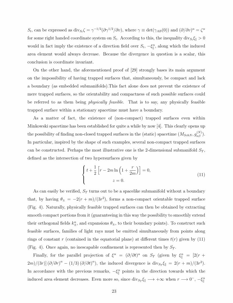
As can easily be verified, ST turns out to be a spacelike submanifold without a boundary

that, by having θ± = −2(r + m)/(3r2), forms a non-compact orientable trapped surface

(Fig. 4). Naturally, physically feasible trapped surfaces can then be obtained by extracting

smooth compact portions from it (guaranteeing in this way the possibility to smoothly extend

their orthogonal fields kα±, and expansions θ±, to their boundary points). To construct such

feasible surfaces, families of light rays must be emitted simultaneously from points along

rings of constant r (contained in the equatorial plane) at different times t(r) given by (11)

(Fig. 4). Once again, no inescapable confinement is represented then by ST .

Finally, for the parallel projection of ξα = (∂/∂t)α on ST (given by ξα‖ = [2(r +

2m)/(3r)] (∂/∂r)α − (1/3) (∂/∂t)α), the induced divergence is divST ξ‖ = 2(r + m)/(3r2).

In accordance with the previous remarks, −ξα‖ points in the direction towards which the

induced area element decreases. Even more so, since divST ξ‖ −→ +∞ when r −→ 0−, −ξα‖

23

FIG. 4: Non-compact trapped surface ST ⊂MSchN .

corresponds in fact to a direction of infinite area contraction along the non-compact trapped

surface ST .

Although a similar divergent behaviour occurs for the trapped surface (within Minkowski

spacetime) of [4], an infinite extent must be traversed for it to be reached. Be-

cause in (MSchN , g(N)αβ ) such contraction coincides with the presence of a scalar/geodesic-

incompleteness singularity, it is suggested here that any extreme behaviour of divStξ‖ could

in fact be used as an indicator of the existence of intrinsic “pathological regions” in a (sta-

tionary) spacetime. That is to say, the existence of (non-closed) trapped surfaces could still

be used to hint the presence of singularities, even if they do not correspond to situations of

inescapable confinement.

On the other hand, it is important to mention that hypothesis (4)(a) of theorem II.2 has

not been taken into consideration due to the fact that its usual physical interpretation allures

only to “closed” universes [28]. Nevertheless, its physical implications will be discussed in

future works for the sake of completeness, together with an analogous analysis for the trapped

submanifolds of co-dimension 3 (i.e. trapped curves) of [6].

V. CONCLUSIONS

This work presents a complete usage of the classical singularity theorems of Penrose (1965)

and Hawking-Penrose (1970). Together with appropriate and illustrative interpretations for

all of their hypothesis, the applicability of the theorems themselves or the mathematical

tools used in them is discussed for the Schwarzschild spacetimes (i.e. the ones with positive

24

and negative mass).

A rigorous treatment for the positive mass case from the point of view of Penrose’s

theorem (that seemingly does not exist so far in the literature), is discussed in detail. As

is expected from the way a spacetime is handled by the theorems, the sole definition of

the Schwarzschild spacetime is enough to guarantee the existence of a singularity by such

theorem. The main result for this case is the validity of the hypotheses of the theorem in a

spacetime that, despite being part of a black hole (i.e. the possible outcome of a process of

complete gravitational collapse), does not contain an event horizon.

For the second case, it is showed the impossibility of using either of the theorems to assure

the existence of singularities. From the proof of such spacetime not being globally hyperbolic,

two conclusions are drawn: (1) there does indeed exist incomplete null geodesics within this

spacetime, and (2) their presence is responsible for the absence of total predictability.

Additionally, it is showed that even though the radial null geodesics of this spacetime are

all non-generic, the temporal nature of their singularity can be better understood from this

fact. Even more so, is it presented with this analysis an example of how the full components

of the tidal stress tensor along such null geodesics, with respect to pseudo-orthonormal bases

adapted to them, could in fact provide information regarding divergent curvature behaviour

in the singularity, as well as its possible repulsive or attractive nature.

In regard to this singularity being naked, agreement is found between the existence of

incomplete null geodesics that extend to infinity, and the absence of regions of inescapable

confinement suggested by a lack of trapped points (and closed trapped surfaces). Further-

more, the occurrence of non-closed trapped surfaces within this spacetime is discussed. It

is argued how despite them not representing scenarios of inevitable confinement, they still

can suggest the existence of singularities in static spacetimes.

Further analysis for these features, in cases of more general static (or even stationary)

spacetimes, will be explored in the future.

Acknowledgements

This work was partially supported by UNAM-DGAPA-PAPIIT, Grant No. 114520,

Conacyt-Mexico, Grant No. A1-S-31269, and by the Ministry of Education and Science

25

(MES) of the Republic of Kazakhstan (RK), Grant No. BR05236322 and AP05133630.

[1] R. Penrose, Phys. Rev. Lett., 14, (1965) 57-59.

[2] J.M.M. Senovilla, D. Garfinkle, Class. Quantum Grav. 32, (2015) 124008.

[3] S.W. Hawking, R. Penrose, Proc. Roy. Soc. Lond. A, 314, (1970) 529-548.

[4] J.M.M. Senovilla, Gen. Relativ. Gravit., 29(5), (1997) 701848.

[5] S. Hawking, Eur. Phys. J. H, 39, (2014) 413-503.

[6] G.J. Galloway, J.M.M. Senovilla, Class. Quantum Grav., 27, (2010) 152002.

[7] M. Eichmair, G.J. Galloway, D. Pollack, J. Differential Geom., 95(3), (2013) 389-405.

[8] I. Bengtsson, J.M.M. Senovilla, Phys. Rev. D, 83, (2011) 044012.

[9] C.J.S. Clarke, Commun. math. Phys., 32, (1973) 205-214.

[10] C.J.S. Clarke, B.G. Schmidt, Gen. Relat. Gravit., 8, (1977) 129-137.

[11] C.J.S. Clarke, J. Math. Anal. Appl., 88(1), (1982) 270-305.

[12] C.J.S. Clarke, The analysis of space-time singularities, Cambridge University Press, USA

(1993).

[13] C.J.S. Clarke, Commun. math. Phys., 41, (1975) 65-78.

[14] C.J.S. Clarke, Commun. math. Phys. 49, (1976) 17-23.

[15] J.A. Thorpe, J. Math. Phys., 18, (1977) 960-964.

[16] J. Kannar, I. Racz, J. Math. Phys. 33(8), (1992) 2842-2848.

[17] A.C. Gutierrez-Pineres, H. Quevedo, Class. Quantum Grav., 36, (2019) 135003.

[18] J.K. Beem, P.E. Ehrlich, K.L. Easley, Global Lorentzian Geometry. 2nd Ed., Marcel Dekker

Inc., USA (1996).

[19] I.P. Costa e Silva, J.L. Flores, Lightlike sets with applications to the rigidity of null geodesic

incompleteness, (2014) arXiv: 1408.4358.

[20] G.J. Galloway, C. Vega, Ann. Henri Poincar, 15, (2014) 2241-2279.

[21] M. Graf, J.D.E. Grant, M. Kunzinger, R. Steinbauer, Commun. Math. Phys., 360(3), (2018)

1009-1042.

[22] K. Maeda, A. Ishibashi, Class. Quantum Grav., 13(9), (1996) 2569-2576.

[23] I.P. Costa e Silva, Class. Quantum Grav., 29(23), (2012) 235008.

[24] J.R. Oppenheimer, H. Snyder, Phys. Rev., 56, (1939) 455-459.

26

[25] P.S. Joshi, Gravitational collapse and spacetime singularities, Cambridge University Press,

UK (2007).

[26] R.M. Wald, V. Iyer, Phys. Rev. D, 44, (1991) R3719(R).

[27] J. Sbierski, J. Differential Geom., 108(2), (2018) 319-378.

[28] S.W. Hawking, G.F.R. Ellis, The large scale structure of space-time, Cambridge University

Press, USA (1994).

[29] M. Mars, J.M.M. Senovilla, Class. Quantum Grav., 20, (2003) L293-L300.

[30] R.M. Wald, General relativity, The University of Chicago Press, USA (1984).

[31] M. Kriele, Spacetime. Foundations of General Relativity and Differential Geometry, Springer-

Verlag, Germany (2001).

[32] R. Engelking, General topology, Heldermann Verlag Berlin, Germany (1989).

[33] L.D. Kudriavtsev, Curso de analisis matematico. Vol.1, Ed. Mir, Moscu, URSS (1983).

27