kimia analitik lanjut
TRANSCRIPT

8/10/2019 Kimia Analitik Lanjut
http://slidepdf.com/reader/full/kimia-analitik-lanjut 1/270
Kimia Analitik Lanjut
Lecturer:
A. Mutalib MSc, PhD

8/10/2019 Kimia Analitik Lanjut
http://slidepdf.com/reader/full/kimia-analitik-lanjut 2/270
IntroductionThree categories of definitions of analytical chemistry:
1. Analytical chemistry produces information by application of available
analytical procedures in order to characterize matter by its chemicalcomposition. This refers to the actual production of analytical results and
requires instruments, procedures, and skilled personnel.
2. Analytical chemistry studies the process of gathering information by using
principles of several disciplines in order to characterize matter or systems.This covers the R&D of analytical procedures.
3. Analytical chemistry produces strategies for obtaining information by the
optimal use of available procedures in order to characterize matter of
systems. This can be considered as an organizational level comprising theinteraction between human and machines, including communication as we
as the optimal use of the tools available for producing information.

8/10/2019 Kimia Analitik Lanjut
http://slidepdf.com/reader/full/kimia-analitik-lanjut 3/270

8/10/2019 Kimia Analitik Lanjut
http://slidepdf.com/reader/full/kimia-analitik-lanjut 4/270
The quality of a sample is given by the similarity between the reconstructi
of the composition of an object and the object itself, as far as it is influenc
by the sampling strategy. It depends on the characteristics of the object and
the purpose of the reconstruction. For a mere description of the object, the quality can be expressed in the
sample quality.
For monitoring of the object, the sampling quality can be expressed as the
probability that a threshold crossing will be detected.
For object control the quality can be expressed as controllability ormeasurability.

8/10/2019 Kimia Analitik Lanjut
http://slidepdf.com/reader/full/kimia-analitik-lanjut 5/270
The limit of detection is a quality parameter pertaining to analysis. It gives
the minimum concentration of a component that can be detected. It is
influenced by the absolute value of the blank, the standard deviation of themethod analysis, a safety factor. The lowest possible limit of detection is s
by the characteristic method.
The sensitivity gives the change of a signal upon a change of concentration
The sensitivity of a method is a practical quality measure, since it pertainsthe ease of detection. However, both the detection of a difference in
concentration between two samples and the limit of detection are ultimatel
governed by the precision of the analytical method and not by sensitivity. T
optimal value of the sensitivity should be such that the standard deviation
the method can be measured.
Quality Parameter

8/10/2019 Kimia Analitik Lanjut
http://slidepdf.com/reader/full/kimia-analitik-lanjut 6/270
Quality Parameter
Selectivity and specificity can be expressed as the ratio of sensitivities of t
method of various components to be measured in the sample. The optimal
value of these characteristics is set by the number of measurements requireto estimate the composition of the sample.
Safety. Perhaps the cost of measures to be taken to satisfy safety regulation
can be used to measure safety as a quality parameter. The optimum is
determined by the balancing of adverse consequences and precaution cost.
Cost can be expressed in money or in other measures, such as manpower.
influenced by analysis time, standard labor, depreciation, and cost of
instruments, energy, and reagents. The optimal cost of an analytical metho
results from a comparison of various methods of analysis with respect toyield of the object and cost of analysis.

8/10/2019 Kimia Analitik Lanjut
http://slidepdf.com/reader/full/kimia-analitik-lanjut 7/270

8/10/2019 Kimia Analitik Lanjut
http://slidepdf.com/reader/full/kimia-analitik-lanjut 8/270
Quality Parameter
Information is defined as the difference in uncertainty before and after an
experiment. It is expressed as the binary logarithm of this uncertainty and
measured in bits.The information content of a qualitative analytical method is governed b
the selectivity and specificity of the method and the a priori knowledge
the occurrence of the sought component.
The information content of a quantitative analytical method is a functio
of the standard deviation of the method and the a priori knowledge of thrange compositions that can be expected.
The information content of a retrieval method is governed by the
selectivity of the method and the chance of occurrence of the sought item
Therefore information cannot be a quality criterion for a method as such
can be applied only in a specified situation. Correlation of items makes a priori information partly predictable and thus diminishes the informati
content of the experiment.

8/10/2019 Kimia Analitik Lanjut
http://slidepdf.com/reader/full/kimia-analitik-lanjut 9/270
Methods Curve fitting is not a quality parameter, but it may enhance the quality of
measured data considerably for two reasons:
1. Interpolating the gap between data allows easier interpretation of many phenomena, although the information does not increase.
2. A most important use of curve fitting is in the unraveling of mixed
phenomena, for example, spectra.
Multivariate analysis may be a tool in establishing new quality criteria. Thfirst application may be in discovering patterns in the data produced by
analytical chemists. This enhances the value of these results. A measure fo
this effect is not known, but a “patterned” result seems to increase the quaof the analytical results.
Optimization is not a quality parameter. However, it may be applied in
optimizing analytical methods and thus improving quality.

8/10/2019 Kimia Analitik Lanjut
http://slidepdf.com/reader/full/kimia-analitik-lanjut 10/270
Techniques to influence or may influence quality Sampling as a means to influence quality. Handling of samples can be of
great importance for some quality aspects of a sample. Homogenizing
influences the quality of the subsample, and so does sample reduction.Preservation and labeling influence both the identity and integrity of the
sample, an immeasurable quality aspect.
Selection of an analytical method may be based on one or more quality
criteria, and therefore these aspects should be weighed a priori. Techniquefor selection are, for example, the ruggedness test, the ranking test, pattern
recognition, optimization, and artificial intelligence.
Repeatability is the measure of variations between test results of successiv
test of the same sample carried out under the same conditions, i.e. the samtest method, the same operator, the same testing equipment, the same
laboratory, and short interval of time..

8/10/2019 Kimia Analitik Lanjut
http://slidepdf.com/reader/full/kimia-analitik-lanjut 11/270
Techniques to influence or may influence quality Reproducibility is the term used to express the measure of variations betw
test results obtained with the same test method on identical test samples
under different conditions, i.e., different operators, different testing
equipment, different laboratories and/or different time.
Precision control and accuracy control. Control chart are means to trace
quality in time and indicate when intervention is required. Round-robin tes
may reveal shortcomings in precision and accuracy and, though complicat
psychological and organizational influences play a role, quality can impro
after test. Sequential analysis as well as analysis of variance may be used t
control precision and accuracy. A number of methods can be used to impro
precision by removing or diminishing irrelevant data (noise). Some
techniques treated are curve fitting and smoothing, Kalman filtering, and
deconvoluting filtering.
Planning
Organization.
li

8/10/2019 Kimia Analitik Lanjut
http://slidepdf.com/reader/full/kimia-analitik-lanjut 12/270
Sampling
Sampling is often called the basis of analysis:
“The analytical result is never better than the sample it is based on”
Every part of the analytical procedure is important, because the final result
influenced by mistakes or added noise in every part procedure.
The purpose of sampling is to provide for a specific aim of the client part
the object that is representative of it and suitable for analysis. The quality of the sampling depends on many parameters, governed by
properties of the object and of the analytical procedure.
The properties of the object can be described in terms of physical
structure, size, and inhomogenicity in space and time.
As a rule the analytical chemist cannot or will not use the whole object in
his/her analysis machine but uses only a small part of the object: ~ 0.01 – 0.1

8/10/2019 Kimia Analitik Lanjut
http://slidepdf.com/reader/full/kimia-analitik-lanjut 13/270
The sample, as a small fraction of the object to be investigated, must fulfill a
series of expectation before it may be called a sample and used as such. It m
• Represent faithfully the properties under investigation: composition, colo
crystal type, etc.
• Be of a size that can be handled by the sampler
• Be of a size that can be handled by the analyst, say, from 0.001 to 1.0 g
• Keep the properties the object had at the time of sampling, or change its
properties in the same way as the object
• Keep its identity throughout the whole procedure of transport and analys
To satisfy these demands, the analyst can use the results of much
theoretical and practical work from other disciplines.
Statistics and probability theory have provided the analyst with the theoretic
framework that predicts the uncertainties in estimating properties of populatiowhen only a part of the population is available for investigation.

8/10/2019 Kimia Analitik Lanjut
http://slidepdf.com/reader/full/kimia-analitik-lanjut 14/270
The properties of analytical procedure can be described in terms of minim
and maximum sample size, physical structure of the sample, homogeneity
the sample in space, and stability in time, for example.
The requirements set by the object and by the analyst must be fulfilled, so sampler has to optimize the sampling parameters such as size, time or
distance spacing, number of subsamples, cost, mixing, and dividing.
The estimation of the value of the properties is the aim of the analytical
procedure. A feature of the object to be known is a list of the desired properties, for these determine the way of sampling.
The object can have many properties, for examples, composition, particle
size, color, and taste, but only selection of these properties is required to
describe the object quality.
Gl f t d i li

8/10/2019 Kimia Analitik Lanjut
http://slidepdf.com/reader/full/kimia-analitik-lanjut 15/270
Glossary of terms used in sampling
Bulk sampling – sampling of a material that does not consist of discrete,
identifiable, constant units, but rather of arbitrary, irregular units.
Gross sample (also called bulk sample, lot sample) – One or more increme
of material taken from a larger quantity (lot) or material for assay or purposes.
Homogeneity – the degree to which a property substance is randomly
distributed throughout a material. Homogeneity depends on the size of the
units under consideration. Thus a mixture of two minerals may be
inhomogeneous at the molecular or atomic level but homogeneous at the particulate level.
Increment – an individual portion of material collected by a single operatio
of a sampling device, from parts of a lot separated in time or space.
Incements may be either tested individually or combined (composited) and
tested as a unit.
Individuals – conceivable constituent parts of the population.
Gl f t d i li

8/10/2019 Kimia Analitik Lanjut
http://slidepdf.com/reader/full/kimia-analitik-lanjut 16/270
Glossary of terms used in sampling
Laboratory sample – a sample, intended for testing or analysis, prepared fro
a gross sample or otherwise obtained. The laboratory sample must retain th
composition of the gross sample. Often reduction in particle size is necess
in the course of reducing the quantity. Lot – a quantity of bulk material of similar composition whose properties a
under study.
Population – a generic term denoting any finite or infinite collection of
individual things, objects, or events in the broadest concept; an aggregate
determined by some property that distinguishes things that do and do not belong.
Reduction – the process of preparing one or more subsamples from a samp
Sample – a portion of a population or lot. It may consist of an individual or
groups of individuals.
Segment – a specifically demarked portion of a lot, either actual or
hypothetical.
Strata – segments of a lot that may vary with respect to the property under
study.
Glossary of terms used in sampling

8/10/2019 Kimia Analitik Lanjut
http://slidepdf.com/reader/full/kimia-analitik-lanjut 17/270
Glossary of terms used in sampling
Subsample – a portion taken from a sample. A laboratory sample may be a
subsample of a gross sample; similarly, a test portion may be a subsample
a laboratory sample.
Test portion (also called specimen, test specimen, test unit, aliquot) – thatquantity of material of proper size for measurement of the property o
interest. Test portions may be taken from the gross sample directly, but oft
preliminary operations such as mixing or further reduction in particle size
necessary.
Types of objects and samples

8/10/2019 Kimia Analitik Lanjut
http://slidepdf.com/reader/full/kimia-analitik-lanjut 18/270
Types of objects and samples
Object
Homogenous
No change of qualitythroughout the object
Heterogeneous
Discrete change of quality
throughout the object
Continuous change of qual
throughout the object
Homogenous Discrete change Continuous change
• Well-mixed liquid
• Well-mixed gases
• Pure metals
Ore pellets
Tablets
Crystallized rocks
Suspensions
oFluids or gases with gradient
o
Mixture of reacting componeoGranulated materials with
granules much smaller than
sample size

8/10/2019 Kimia Analitik Lanjut
http://slidepdf.com/reader/full/kimia-analitik-lanjut 19/270
The discrete or continuous changes in object quality can manifest themselv
in time as well as in space.
The composition of the output of a factory changing with time can be seen
a time-related property by sampling the output. It can be seen as a space-
related property by sampling the conveyor belt or the warehouse.
A special type of heterogeneous object exhibits cyclic changes of its
properties. Frequencies of cyclic variations can be a sign of daily influence
as temperature of the environment or shift-to-shift variations. Seasonalfrequencies are common in environmental objects like air or surface water
These several types of heterogeneous objects are seldom found in their
pure state, mixed forms with one or two dominating types are most
common.
The object

8/10/2019 Kimia Analitik Lanjut
http://slidepdf.com/reader/full/kimia-analitik-lanjut 20/270
The object
“The entity to be described”
An object can be a fertilizer granule as well as a bag or truckload of
fertilizer , or even the quantity produced last week.
As a rule the object is sufficiently described by the four coordinates of
space and time, though in practice other labels may be more useful. Oth
state variable temperature and pressure, for often the sample cannot be
kept in the same condition.
Sample nomenclature
8/10/2019 Kimia Analitik Lanjut
http://slidepdf.com/reader/full/kimia-analitik-lanjut 21/270
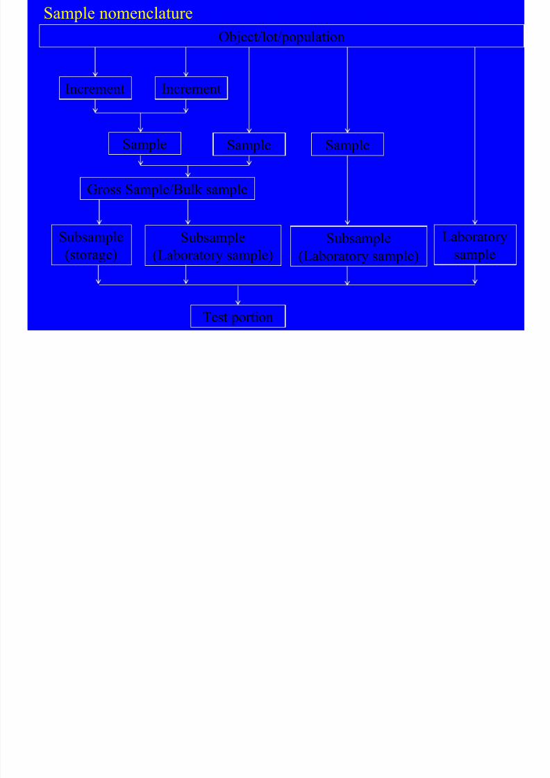
Sample nomenclature
Object/lot/population
Increment Increment
Sample Sample Sample
Gross Sample/Bulk sample
Subsample
(storage)
Subsample
(Laboratory sample)
Laborator
sampleSubsample
(Laboratory sample)
Test portion
The Sample

8/10/2019 Kimia Analitik Lanjut
http://slidepdf.com/reader/full/kimia-analitik-lanjut 22/270
The Sample“A representative part of the object to be analyzed”
Because representativeness is needed only for the object quality paramete
it can also be stated, “A sample is part of the object selected in such a waythat it possesses the desired properties of the object”
A sample the size of a truckload can be a good sample – that is,
representative of the object- but it cannot be used in the laboratory. A very
small sample can be as good a sample as a larger one, but perhaps it is
impossible to handle.
“The sample must have such dimensions that it can be analyzed.”
The sample must keep the properties the object had at the time of samplingor change its properties in the same way as the object. Thus deterioration
the sample through exposure to the air, the sample container, or
microorganism, for example, should be avoided.
Principles of sampling

8/10/2019 Kimia Analitik Lanjut
http://slidepdf.com/reader/full/kimia-analitik-lanjut 23/270
Principles of sampling
The purpose of most measurements, and especially chemical measuremen
is to evaluate some property of a material of interest. The value of the
property is then used in a decision process to make judgments on such
questions as its suitability for a specific use, the need for some correctiveaction, or the conformance with some specification.
The samples measured are often the most critical aspect of a measurement
program. They must be relevant and truly represent the universe concern.
In limited cases, the specimen tested is the universe concern. For example
forensic analysis the identification of a single chip of metal could be decis
for settling a legal question.
In most cases, the specimen tested are only a part of the universe of conceThen, it is extremely important to know how the specimen are related to th
universe since the decision process is concerned with the universe and not
with the specimens tested.
Items for consideration when developing a sampling plan

8/10/2019 Kimia Analitik Lanjut
http://slidepdf.com/reader/full/kimia-analitik-lanjut 24/270
Type of
Sample
Items for consideration when developing a sampling plan
Identification
of population
Chain of
custody
Sample
Number
of sample
Size of
sample
Sampling
SOP
Sampling
calibration
Sample
treatment
containment
Subsampling Storage
holding time
Initial Consideration

8/10/2019 Kimia Analitik Lanjut
http://slidepdf.com/reader/full/kimia-analitik-lanjut 25/270
Initial Consideration
The first problem is to identify the universe of concern. There must be a
clear conception of what is to be sampled; hence, the physical, chemical,
and dimensional parameters that define it must be known.
Three kind of universes:
1. Single item, in which the entire universe is evaluated;
2. Discrete lot, consisting of a finite number of discrete individuals, e.g..,
items from a production lot;
3. Bulk, a massive material composed of arbitrary and/or irregular units.A “defined bulk” is one in which the boundaries are clearlydistinguishable while a “diffuse bulk” is one which the limits are ill-defined.
The compositional makeup needs to be considered. Can the universe be
considered to be homogenous? That is to say, can every conceivable sampl
be said to have essentially the same composition, or is the composition
ex ected to var ?
Initial Consideration

8/10/2019 Kimia Analitik Lanjut
http://slidepdf.com/reader/full/kimia-analitik-lanjut 26/270
Initial Consideration
The question of stability of composition needs to be considered in some
cases. The composition of a sample may change once it is removed from it
natural matrix or environment, due to kinetic effect or interaction with a
container, radiation, or air, for example. It may need to be stabilized ormeasured within some safe holding period.
It is necessary to know:
• What substances are to be measured
• What level of precision is required• What compositional information is needed
− Mean composition
− Extremes of composition
− Variability of composition
Purpose of sampling

8/10/2019 Kimia Analitik Lanjut
http://slidepdf.com/reader/full/kimia-analitik-lanjut 27/270
Purpose of sampling
The sample procedure, or sampling, is a succession of steps performed on
object ensuring that a sample possesses the specified sample quality.
Because the particular sample procedure depends on the purpose of sampl
the various purposes must be delineated.
One purpose of sampling may be collection of a part of the object that is
sufficient for the gross composition of the object, for example, sampling
lots of a manufactured product, lots of raw material, or the mean state of
process. It is desirable to collect a sample that has the minimum size set b
the condition of representative or demanded by handling.
A second purpose of sampling can be the detection: drift or cyclicvariations. Special techniques are required to discover such anomalies as
soon as possible. These also set the condition for sampling frequency and
sample size.

8/10/2019 Kimia Analitik Lanjut
http://slidepdf.com/reader/full/kimia-analitik-lanjut 28/270
Sampling Plan

8/10/2019 Kimia Analitik Lanjut
http://slidepdf.com/reader/full/kimia-analitik-lanjut 29/270
p g
There are basically three kinds of sampling plans that can be used in a
measurement process:
1. Intuitive sampling plans may be defined as those based on the judgment of
the sampler. General knowledge of similar materials, past experience, and present information about the universe of concern, ranging from knowledg
to guesses, are used in devising such sampling plans. In the case of
controversy, decisions on acceptance of conflicting conclusions may be ba
on the perceived relative expertise of the those responsible for sampling.
2. Statistical sampling plans are those based on statistical sampling of the
universe of concern and ordinarily can provide the basis for probabilistic
conclusions. Hypothesis testing can be involved, predictions can be made,
and inferences can be drawn. Ordinarily, a relatively large number of samp
will need to be measured if the significance of small apparent differences iof concern. The conclusion drawn from such samples would appear to be
non-controversial, but the validity of statistical model used could be a matt
of controversy.
Sampling Plan

8/10/2019 Kimia Analitik Lanjut
http://slidepdf.com/reader/full/kimia-analitik-lanjut 30/270
p g
3. Protocol sampling plans may be defined as those specified for decision
purposes in a given situation. Regulation often specify the type, size,
frequency, sampling period, and even location and time of sampling relate
to regulatory decisions. The protocol may be based on statistical or intuiticonsiderations but is indisputable once established. Testing for conforman
with specifications in commercial transactions is another example.
Agreement and definition of what constitutes a valid sample and the meth
of test are essential in many such cases.
When decision are based on identifying relatively large differences,
intuitive samples may be fully adequate. When relatively small
differences are involved and the statistical significance is an issue,
statistical sampling will be required.
When the number of samples required by a statistical sampling plan ma be infeasible, a hybrid plan involving intuitive simplifying assumption
may be used.
Sampling Plan

8/10/2019 Kimia Analitik Lanjut
http://slidepdf.com/reader/full/kimia-analitik-lanjut 31/270
p g
Whatever kind of sampling plan is developed, it should be written as a protoco
containing procedures (SOPs) that should be followed. It should address:
When, where, and how to collect samples
Sampling equipment, including its maintenance and calibration
Sample containers, including cleaning, addition of stabilizers, and storage
Criteria for acceptance and/or rejection of samples
Criteria for exclusion of foreign objects Sample treatment procedures such as drying, mixing, and handling prior to
measurements
Subsampling procedures
Sample record keeping such as labeling, recording, and auxiliary informat
Chain of custody requirements

8/10/2019 Kimia Analitik Lanjut
http://slidepdf.com/reader/full/kimia-analitik-lanjut 32/270
Systematic Deviations in Sampling

8/10/2019 Kimia Analitik Lanjut
http://slidepdf.com/reader/full/kimia-analitik-lanjut 33/270
Some causes of systematic deviations in sampling are the following:
1. The number increments is too small, so that the sample shows a bias. In fac
this is a random deviation.2. The sampling procedure is preferential to one or more object quality
parameters.
3. The sampling procedure causes alterations in the object.
4. The sample changes after the sampling procedure and before the analysis.
5. The sample is altered intentionally.
Sampling parameters
8/10/2019 Kimia Analitik Lanjut
http://slidepdf.com/reader/full/kimia-analitik-lanjut 34/270
M
G1 G2 G3
A
P
t
x
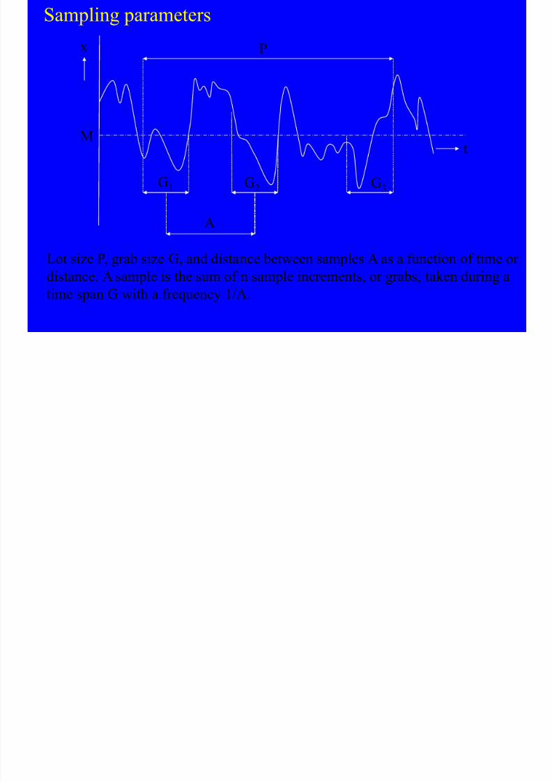
Lot size P, grab size G, and distance between samples A as a function of time
distance. A sample is the sum of n sample increments, or grabs, taken during
time span G with a frequency 1/A.
Samples for Gross Description

8/10/2019 Kimia Analitik Lanjut
http://slidepdf.com/reader/full/kimia-analitik-lanjut 35/270
Homogenous objects
If the object to be sampled is homogenous, for example, a well-mixed ta
or lake, it is obvious that here every sample, whatever its size, is a true
copy of the object.
Theoretically one sample suffices. Often in practice more samples are
needed, for instance, to fulfill the requirement that the sample must have
minimum size.
When the sample size too large, such as in precious objets d’art, more
sample are needed.
The size of the gross sample, set by the requirements of the analysis, can
be estimated as follows: assume the sample weight W and the fraction othe component to be estimated is P (1% → P = 0.01; 1 ppm → P = 10-6)
The total amount of component in the sample is T = PW

8/10/2019 Kimia Analitik Lanjut
http://slidepdf.com/reader/full/kimia-analitik-lanjut 36/270
Samples for Gross Description

8/10/2019 Kimia Analitik Lanjut
http://slidepdf.com/reader/full/kimia-analitik-lanjut 37/270
Heterogeneous objects
The cause of difference between the increment and the object is the
inevitable statistical error in taking an increment from the object. Thecomposition of the grab, the collection of increments that must ultimate
constitute a sample, is given by m and s, with m being the mean
composition of the object and s the standard deviation of this mean.
From statistics it is known that s = ( P A P Bn)1/2 particles or
where s g = standard deviation of the increment P A = fraction of component A in the object
P B = 1 – P A = fraction of component B in the object
n = number of particles.
Samples for Gross Description

8/10/2019 Kimia Analitik Lanjut
http://slidepdf.com/reader/full/kimia-analitik-lanjut 38/270
Heterogeneous objects
Assume the same composition as before, 50% A, 50% B, P A = 0.50, and
P B = 0.50. An increment with n = 10 will have composition
m = 50% A;
Two out of three increments will have a composition between 50± 16%or 3 and 7 particles A. The probability that an increment is found outsid
this region is 1 : 3. In fact, the probability of finding an increment with t
composition 10 particles A or B is not negligible: 1% of the increments
will have a composition of 0 or 10 particles of one kind.
Samples for Gross Description

8/10/2019 Kimia Analitik Lanjut
http://slidepdf.com/reader/full/kimia-analitik-lanjut 39/270
Heterogeneous objects
If the increment is considered to be representative of the object, when
there is no means to distinguish this increment from another one take
from the object, a method of analysis is required that has an ultimateaccuracy larger than the standard deviation of the increment. When th
accuracy of the analysis is
where sa = standard deviation of the analysis
s A = standard deviation of the method of analysis
N = number of repeated analysis
No distinction can be found between two increments provided s g < sa
(it is known a priori that an increment will not be equal to the object.
This is not important, however, if the difference cannot be seen)
Samples for Gross Description

8/10/2019 Kimia Analitik Lanjut
http://slidepdf.com/reader/full/kimia-analitik-lanjut 40/270
Heterogeneous objects
The condition set for an increment to be a sample is s g ≤ sa or
which is equivalent to
It is described by Visman that the sampling variance as the sum of
random and segregation compounds according to
A and B are constants determined by preliminary measurements on the
system. The A term is the random component; its magnitude depends on
the weight w and the number n of sample increments collected, the sizeand variability of the composition of the units in the population. The B
term is the segregation component and depends only on the number of
increments collected and on the heterogeneity of the population.
Samples for Gross Description Heterogeneous objects

8/10/2019 Kimia Analitik Lanjut
http://slidepdf.com/reader/full/kimia-analitik-lanjut 41/270
Heterogeneous objects
Another way to estimate the amount of samples that should be taken
a given increment so as not to exceed a predetermined level of sampl
uncertainty is via the use of Ingamells‟s sampling constant
where W represents the weight of sample; R is the relative standard
deviation (in percent) of the sample composition; and K s is the sampling
constant (Ingamells‟s sampling constant), the weight of sample required
limit the sampling uncertainty of 1% with 68% confidence. The magnitu
of K s may be determined by estimating the standard deviation from a se
of measurements of samples of weight W.
Samples for Gross Description

8/10/2019 Kimia Analitik Lanjut
http://slidepdf.com/reader/full/kimia-analitik-lanjut 42/270
Sampling diagram of sodium-24 in human liver homogenate.
K s
0.1 1 10
1.7
2.1
2.5
2.7
Sample weight, g
C o u n t s , g - 1 . s
- 1 . 1
0 - 2
Samples for Gross Description

8/10/2019 Kimia Analitik Lanjut
http://slidepdf.com/reader/full/kimia-analitik-lanjut 43/270
Gy introduced a shape factor f as the ratio of the average volume of
particles having a maximum linear dimension equal to the mesh size
a sieve to that of a cube which will just pass the same screen:
f = 1.00 for cubes; f = 0.524 for spheres; f ~ 0.5 for most materials.
The particle size distribution factor g is the ratio of the upper size lim
(95% pass screen) to the lower size limit (5% pass screen). For
homogeneous particle size g = 1.00. The composition factor c is
where x is the overall concentration of the component of interest; d xthe density of this component and d g the density of the matrix
(remaining components); c is in the range 5 x 10⁻⁵ kg/m3 for highconcentrations of c to 103 for trace concentrations.
Samples for Gross Description Th lib i f l i

8/10/2019 Kimia Analitik Lanjut
http://slidepdf.com/reader/full/kimia-analitik-lanjut 44/270
The liberation factor l is
where d l is the mean diameter of the component of interest, and d th
diameter of the largest particles. The standard deviation of the samp
s is estimated by
Ingamells related Gy‟s sampling constant to Ingamells‟s constant by
Samples for Gross Description I t ll C l t d Obj t

8/10/2019 Kimia Analitik Lanjut
http://slidepdf.com/reader/full/kimia-analitik-lanjut 45/270
Objects can be internally correlated in time or space; for example, the
composition of a fluid emerging from a tank does not show random flu
tuations but is correlated in the composition earlier or later sampled product. When the object is internally correlated, no distinct boundaries ex
Factors causing the internal correlation of objects include:
diffusion or mixing within the object, for example, in mixing tanks,
buffer hoppers, and rivers
varying properties of producer of the object, for example, reactors oemitters
When an objects shows a large internal correlation, two adjacent samp
do not differ much from each other. However, the difference between t
samples increases with greater distance. For the case of heterogeneous
objects, the number of increments n depends on the required variance othe sample, this variance being so small that the difference between tw
samples cannot be detected..
Internally Correlated Objects
Samples for Gross Description Internally Correlated Objects

8/10/2019 Kimia Analitik Lanjut
http://slidepdf.com/reader/full/kimia-analitik-lanjut 46/270
Internally Correlated Objects
When the object to be analyzed is a process, a stream of material of
infinite length with properties varying in time, the sampling parameters
can be derived from the process parameters.
When the object is a finite part of a process, however, usually called a
lot, the description of the real composition of the lot depends not only
the parameters of the process the lot is derived from but also on the len
of the lot. The sample now must represent the lot, not the process.
Lots derived from Gaussian, stationary, stochastic processes of the firs
order allow a theoretical approach. In practice most lots seem to fulfill
above requirements with sufficient accuracy; an estimate of the mean m
of a lot with size P can be obtained by taking n samples of size G, equaspaced with a distance A; in this case P = nA and the size of the gross
sample S = nG. Here it is assumed that it is not permissible to have
overlapping samples and that A → G.

8/10/2019 Kimia Analitik Lanjut
http://slidepdf.com/reader/full/kimia-analitik-lanjut 47/270
Samples for Gross Description Internally Correlated Objects

8/10/2019 Kimia Analitik Lanjut
http://slidepdf.com/reader/full/kimia-analitik-lanjut 48/270
Internally Correlated Objects
where
T x = correlation factor of the process
n = number of samples
The only relevant property of the lot here its size p, expressed in unitsThese units may be times units, such as when T x is measured in hours.
this case T x is usually called the time constant of the process. The lot si
is expressed in hours as well. When a river is being described, the lot
can be the mass of water that flows by in 1 day or year.
The correlation factor T x can be called a space constant, however, when
the unit used is of length. Here the lot size is expressed length units.
Samples for Gross Description Internally Correlated Objects

8/10/2019 Kimia Analitik Lanjut
http://slidepdf.com/reader/full/kimia-analitik-lanjut 49/270
te a y Co e ated Objects
This is the case, for example, when a lot of manufactured products
contained in a conveyor belt or stored in a pile of material in a warehou
is considered. The values of P, G, and A can be expressed indimensionless units when they are divided by T x.
The correlation factor can also be expressed in dimensionless units, as
when bags of products are produced. In this case the lot size is express
in terms of item as well (number of bags, drums, tablets).
The properties of the sample are increment size g, expressed in the sam
units as T x, and p, the distance between the middle of adjacent increme
a and the number of increments n that form the sample. If the sample
is expressed as a fraction of the object P ( F = G/P ), the relations betwe F and n are depicted in Figure below for a certain value of s x.
1

8/10/2019 Kimia Analitik Lanjut
http://slidepdf.com/reader/full/kimia-analitik-lanjut 50/270
0.01 0.1 1 10 100 1000 100
0.01
0.1
1
F & n F
Figure The relative sample size F (−) and the relative gross sample size nF (
a function of the relative lot size p for various numbers of sample (s * /s x)
p

8/10/2019 Kimia Analitik Lanjut
http://slidepdf.com/reader/full/kimia-analitik-lanjut 51/270
Sample uncertainties
T t l i i t f th f th t d t th l d t th i

8/10/2019 Kimia Analitik Lanjut
http://slidepdf.com/reader/full/kimia-analitik-lanjut 52/270
Total variance consists of the sum of that due to the samples and to their
measurement.
It is the variance of the sample population that is of most concern when
answering questions by measurement. The variance of the samples measur
is related to that of the population and sampling by the expression:
It is good advice to take all the care necessary to make sampling variance
negligible.
Some measurement programs require ancillary data such as pressure,
temperature, flow, and moisture content, to reduce the data to standardconditions. Both random and systematic errors in measurement of these
parameters can reflect similar sources of error in the measurement data.
s2total = s2
sample + s2measurement
s2
sample
= s2
population
+ s2
sampling
Sample uncertainties
St tifi ti hen possible is an insidio s so rce of error in

8/10/2019 Kimia Analitik Lanjut
http://slidepdf.com/reader/full/kimia-analitik-lanjut 53/270
Stratification
Sample that were initially well-mixed may separate, partially or fully, over
period of time. It may be difficult (perhaps impossible) to reconstitute them
and even the need to do so may not be apparent.
when possible, is an insidious source of error in
analytical sample
Examples: a mixture of solids that may be separate due to gravitational
and/or vibrational forces
emulsions that could demulsify water samples containing suspended matter that later could
plate out on container wall
Whenever stratification is possible, care should be exercised to reconstitute the sample, to
the extent possible, each time a subsample is withdrawn. Otherwise, problems caused by
poor mixing can become even more serious as the ratio of sample increment to residualsample increase.
Any apparent uncompensated uncertainties resulting from segregation in its various aspec
should be considered when evaluating measurement data.
Sample uncertainties
Holding time the maximum period of time that can elapse from samp

8/10/2019 Kimia Analitik Lanjut
http://slidepdf.com/reader/full/kimia-analitik-lanjut 54/270
Holding time the maximum period of time that can elapse from samp
to measurement before significant deterioration can
expected to occur. When degradation is possible, samp
should be measured before any significant change occur
Max Holding Time
M e a s u r e d
C o n c e n t r a t i o n
C0 Time
Lower Limit
.
If the holding time is considered to be inconveniently short, the conditions ofstorage and/or stabilization must be modified necessitating a new determinatio
of holding time. Very transitory samples may need to be measured immediatel
after sampling.
Statistical Considerations for Sampling
Measurement Situations

8/10/2019 Kimia Analitik Lanjut
http://slidepdf.com/reader/full/kimia-analitik-lanjut 55/270
Measurement Situations
Significant Not Significant
A. Measurement Variance X
Sample Variance X
B. Measurement Variance X
Sample Variance X
C. Measurement Variance X
Sample Variance X
D. Measurement Variance X
E. Sample Variance X
Situation A is the most desirable but is seldom encountered. In this case, a
single measurement on a single sample could provide all of the information
required to make a decision. Situation B can be known in advance when the measurement system is in
statistical control, hence a single measurement of a representative sample
be used for decision ur ose.
Statistical Considerations for Sampling
Measurement Situations

8/10/2019 Kimia Analitik Lanjut
http://slidepdf.com/reader/full/kimia-analitik-lanjut 56/270
Measurement Situations
Situation C is more complex in that more than one sample measurement w
be needed in order to relate the data to the universe of interest.
Situation D occurs frequently, especially in environmental analysis. Asampling plan, involving multiple samples, will be needed as in C
Statistical Sampling Plan
Statistics can provide several kinds of information in the development of
sampling plans and the evaluation of measurement data, including:.
The limit of confidence for the measured value of the population mean
The tolerance interval for a given percentage of the individuals in the
population The minimum number of samples required to establish the above interva
with a selected confidence level
Statistical Sampling Plan
S l diti th t t b t h ki t ti ti l ti t

8/10/2019 Kimia Analitik Lanjut
http://slidepdf.com/reader/full/kimia-analitik-lanjut 57/270
Several conditions that must be met when making statistical estimates:
o The samples must be randomly
selected from the population of
concern
o Each sample must be independent
of any other of sample in the
group
o The type distribution of the
sample must be known, in order
to apply the correct statistical
model.
Could be realized by a samplingoperation that employs a
randomization process and assuranc
that one sample does not influence
another, such as cross-contamination
A Gaussian distribution is often
applicable, or assumed, and such
statistics are easiest to apply.
Basic Assumptions
For statistical planning an estimated or assumed standard deviation is trea

8/10/2019 Kimia Analitik Lanjut
http://slidepdf.com/reader/full/kimia-analitik-lanjut 58/270
For statistical planning, an estimated or assumed standard deviation is trea
as if it were the population standard deviation.
For statistical calculations, the standard deviation estimate, s, based onmeasurement data, is used in the conventional manner.
In the analysis of variance from several sources, it is assumed that the total
variance is equal to the sum of the various components:
s20 = s2
1 + s22 + ……. + s2
n
In sampling it is used the notation
sA = standard deviation of measurement
ss = standard deviation of samples (within a stratum) sB = standard deviation of between strata
Guidance in Sampling
The minimum number of samples and/or measurements necessary to limit

8/10/2019 Kimia Analitik Lanjut
http://slidepdf.com/reader/full/kimia-analitik-lanjut 59/270
The minimum number of samples and/or measurements necessary to limit
total uncertainty, to a value E, with a stated level of confidence ( a value z)
For the 95% level of confidence, z = 1.96 ≈ 2
a. Minimum Number of Measurement, nA (ss negligible)
In the above calculation, if nA is more than is considered to be feasible:
• improve the precision of the methodology to decrease sA, or
•
use a more a precise method of measurement if available (smaller sA)• Accept a larger uncertainy.
(Measurement Situation B)
Guidance in Sampling

8/10/2019 Kimia Analitik Lanjut
http://slidepdf.com/reader/full/kimia-analitik-lanjut 60/270
b. Minimum Number of Measurement, ns (sA negligible)
If more samples are required than is feasible:
• use larger sample (smaller ss), or
• use composites (smaller ss), or
• accept a larger uncertainty
(Measurement Situation C)
Guidance in Sampling
c When sA and s both are significant

8/10/2019 Kimia Analitik Lanjut
http://slidepdf.com/reader/full/kimia-analitik-lanjut 61/270
c. When sA and ss both are significant
where nA is the number of measurements per sample.
• The equation above has no unique solution in that several values of
and nA will produce the same value of E.• Compromises will be necessary, taking into consideration the costs o
sampling and of measurement. The nomographs of Provost (Provos
L.P., Statistical Methods in Environmental Sampling for Hazardous
Wastes, ACS Synposium Series 267, ACS, Washington, DC 20036
(1984)) may be helpful in making the various estimates.• The ways to decrease ss and/or sA will decrease the number of
samples and/or measurements required.
(Measurement Situation D)
Guidance in Sampling

8/10/2019 Kimia Analitik Lanjut
http://slidepdf.com/reader/full/kimia-analitik-lanjut 62/270
• When samples come from several strata
Where nB = number of strata sampled
ns = number of samples per strata• No unique solution is possible so that compromises will be required
Cost Consideration
U ll it i t d i li l ith t id ti

8/10/2019 Kimia Analitik Lanjut
http://slidepdf.com/reader/full/kimia-analitik-lanjut 63/270
Usually, it is necessary to design a sampling plan with cost considerations
mind.
Let
It can be shown that
ns
nA
Cs
CA
C
C
= total number of samples
= number of measurements per sample
= cost per sample of sampling
= cost per measurement
= total cost of program
= ns
Cs
+ ns
nA
CA

8/10/2019 Kimia Analitik Lanjut
http://slidepdf.com/reader/full/kimia-analitik-lanjut 64/270
Minimum Size of Increments in a Well-Mixed Sample In the case of heterogeneous solids, it is well-known that variability betwee
i i h i i d

8/10/2019 Kimia Analitik Lanjut
http://slidepdf.com/reader/full/kimia-analitik-lanjut 65/270
increments increases as their size decreases.
It has been shown by Ingamells that the following relation is valid in many
situations.
WR 2 = K s
where W = weight of sample analyzed, g
R = relative standard deviation of sample composition, %K s = sampling constant, required to limit the sampling uncertainty t
1% with 68% confidence.
Once K s is evaluated for a given sample population, the maximum weight,
required for a maximum relative standard deviation of R percent can be
calculated. If the material sampled is well mixed, the relationship holds verwell. For segregated or stratified materials, the calculated value for K s
increases as W increases. This is one way that the degree of mixing can be
judged.
Size of Sample in Segregated Materials
In the case of segregated materials, it has been shown by Visman that the

8/10/2019 Kimia Analitik Lanjut
http://slidepdf.com/reader/full/kimia-analitik-lanjut 66/270
g g y
variance of sampling, s2s may be expressed by the relation
where A = random component of sampling variance
B = segregation component
W = weight of individual increment, g
n = number of increments
The error due to random distribution may be reduced by increasing W and/
n.
Doubling the number of increments has the same effect as doubling theweight of each increment. However, the error due to segregation is reduced
only by increasing the number of increments sampled.
Size of Sample in Segregated Materials
The constraints A and B must be evaluated experimentally. One way to do

8/10/2019 Kimia Analitik Lanjut
http://slidepdf.com/reader/full/kimia-analitik-lanjut 67/270
is to collect a set of large increments, each of weight WL, and a set of small
increments, each of weight WS. Each set is measured and the respective
standard deviation, sL and sS are calculated. Then
The degree of segregation
The values for zS > 0.05 can cause serious errors in the estimation of sS if thsingle sampling constant approach is used.
Acceptance Testing Acceptance testing is based on judging whether a lot of material meets
t bli h d ifi ti

8/10/2019 Kimia Analitik Lanjut
http://slidepdf.com/reader/full/kimia-analitik-lanjut 68/270
preestablished specifications.
• Involving decisions on whether a material tested meets a compositiona
specification such as the carbon content of a cast iron If a representative sample is to be used as the basis for decision, it m
be defined in the plan.
If multiple samples are to be used, then the number, size, and metho
of collection need to be specified.
The permissible variability of material (homogeneity) is oftenimportant and decisions on conformance require statistical sampling
• Consisting in the extent or fraction of defective (out-of-specification)
items in a lot.
The determination of whether the observed percentage of defectivessignificant and exceeds some specified value requires statistical
sampling of the material in question.
Matrix-Related Sampling Problems Sampling Gases
G id d t b i h h th b f
8/10/2019 Kimia Analitik Lanjut
http://slidepdf.com/reader/full/kimia-analitik-lanjut 69/270
Gases are considered to be microhomogeneous, hence the number of
samples required is related largely differences due to time and location of
sampling. Gases in the atmosphere can be stratified due to emission from point sour
and to differences in density components.
Mixing by diffusion, convection, and mechanical stirring can be more
inefficient than might be imagined. When gas blends are prepared in
cylinders, it can take considerable time for the mixture to equilibrate for tsame reasons
Environmental gas analysis often involves real-time measurement of
samples extracted from the atmosphere. The siting of monitoring stations
a critical aspects of such measurements. The possible degradation of
samples during transit in sampling lines also needs to be considered. Sampling may consist of absorbing some component of interest from an
atmosphere in order to concentrate it to measurable levels or for
convenience of later measurement.
Matrix-Related Sampling Problems Sampling Gases
Gas sampling can consist of collecting a portion in a container The

8/10/2019 Kimia Analitik Lanjut
http://slidepdf.com/reader/full/kimia-analitik-lanjut 70/270
Gas sampling can consist of collecting a portion in a container. The
possible interaction of components with the walls of the container and al
the possible deterioration and/or interaction of constituents need to be
considered.
Grab samples of gases may be collected by opening a valve of a previou
evacuated container. Composite samples may be obtained by intermitten
opening the valve for predetermined intervals, selected to obtain equal
increments of gas, based on pressure drop considerations.
Gas samples are sometimes collected by condensation in a refrigerated t
One must remember that the composition of gas evolved on warming ca
vary due to differential evaporation unless the entire sample is evaporate
before withdrawal of any part of it. The same problem can be encounter
in withdrawal of the contents of a cylinder gas containing easily condens
components.
Matrix-Related Sampling Problems Sampling Liquids

8/10/2019 Kimia Analitik Lanjut
http://slidepdf.com/reader/full/kimia-analitik-lanjut 71/270
What has been said about gases applies in principle to the sampling of
liquids.
The concept of holding time is especially applicable to liquids and
especially to aqueous samples.
Liquid samples are often large, to provide the possibility of multiparame
measurement.
Methods of transport need to be considered to minimize breakage and lo
of contents. Sample may appear to be homogenous, but phase separation
can occur as a result of temperature changes, freezing, or long standing.
When such occur, it may be impossible to fully reconstitute the sample.
Matrix-Related Sampling Problems Sampling Solids

8/10/2019 Kimia Analitik Lanjut
http://slidepdf.com/reader/full/kimia-analitik-lanjut 72/270
The methods used to obtained solid samples depend on whether the
material is massive, consists of aggregates, or is fine granular.
Heterogeneity is a common characteristic, and the statistical sampling
should be considered.
Questions of stability ordinarily are not of major concern, but air oxidati
and/or moisture interactions can cause problems, especially for fine groumaterials with large surface areas.
Matrix-Related Sampling Problems Sampling Multiphases

8/10/2019 Kimia Analitik Lanjut
http://slidepdf.com/reader/full/kimia-analitik-lanjut 73/270
All of the possible combinations – liquid-solid, liquid-gas, solid-gas, liqu
liquid, solid-solid, and liquid-solid-gas- can be encountered. The samplin
plan applicable will depend on whether a specific analyte, a single phasecomplete analysis, or any variation of the above is of concern.
Once a sample has been obtained and/or removed from its normal
environment, the possibility of phase changes and disruption of phase
equilibria must be considered and addressed as necessary. There can bechanges due to differential volatility, absorption, settling of suspended
matter, demulsification, and related physical and chemical effects that
could change a sample drastically.
In some cases, the phase of interest is separated from its matrix or carrie phase prior to measurement
Principles of MeasurementTerminology

8/10/2019 Kimia Analitik Lanjut
http://slidepdf.com/reader/full/kimia-analitik-lanjut 74/270
Technique – a scientific principle that has been found useful for providi
compositional information
Method – an adaptation of a technique to a specific measurement
problem
Procedure – the written direction considered to be necessary to utilize a
method
Protocol – a set of definitive instructions that must be followed, withoexception, if the analytical results are to be accepted for a
specific purpose
The hierarchy of methodology: technique – method - procedure - protocol
Principles of MeasurementTerminology
Absolute Method – method in which characterization is based

8/10/2019 Kimia Analitik Lanjut
http://slidepdf.com/reader/full/kimia-analitik-lanjut 75/270
entirely on physical (absolute) standards.
Comparative Method – method in which characterization is based o
chemical standards (i.e., comparison with su
standards)
Reference Method – a method of known and demonstrated
accuracy.
Standard Method – a method of known and demonstrated precis
issued by an organization generally recogniz
as competent to do so.
Standard Reference Method – a standard method of demonstrated accura
Definitive Method – a method of known accuracy that has been
accepted to establish the property of some
material (e.g., reference material) and/or to
evaluate the accuracy of other methodology
(term widely used in clinical analysis).
Principles of MeasurementTerminology

8/10/2019 Kimia Analitik Lanjut
http://slidepdf.com/reader/full/kimia-analitik-lanjut 76/270
Routine Method – method used in routine measurement of a
measurand. It must be qualified by other
adjectives since the degree reliability is not
implied.
Comparative Method – method in which characterization is based o
chemical standards (i.e., comparison with su
standards)
Field Method – method applicable to nonlaboratory situation
Trace Method – method applicable to ppm range.
Ultra Trace Method – method applicable below trace level.
Macro Method – method requiring more than milligram amou
of sample.
Micro Method – method requiring milligram or smaller amou
of sample.
Table Classes of Methods

8/10/2019 Kimia Analitik Lanjut
http://slidepdf.com/reader/full/kimia-analitik-lanjut 77/270
Class Precision/Accuracy (P/A) Nomenclature
A < 0.01% Highest P/A
B 0.01 – 0.1% High P/A
C 0.1 – 1% Intermediate P/A
D 1 – 10% Low P/A
E 10 – 35% Semiquantitativ
F > 35% Qualitative
Structure of an Analytical Procedure It consists of six distinguishable steps:

8/10/2019 Kimia Analitik Lanjut
http://slidepdf.com/reader/full/kimia-analitik-lanjut 78/270
Sampling
Sample preparation
Measuring
Data processing
Testing, controlling, and eventually correcting one or more of
the processing stages
Establishing a quality merit
Structure of an Analytical Procedure No analytical procedure is complete without a proper validation of each o
the stages and of the final result.

8/10/2019 Kimia Analitik Lanjut
http://slidepdf.com/reader/full/kimia-analitik-lanjut 79/270
g
Based on type of measurements, analytical processes can be divided into
one-dimensional and two-dimensional methods.
Measurement is basically a comparison of an unknown with a known.
Direct comparison, as in determination of mass using an equal-arm
balance
Indirect comparison, as in determination of mass using a spring balanc
Except for the assay of pure substances, the constituent(s) of interest is
usually contained in a matrix that may or may not influence its
measurement. Some measurements can be made in the native matrix with
little or no modification thereof. Emission spectroscopy is an example of
this.
Structure of an Analytical Procedure In others, a modifier may be added to facilitate the measurement or to
provide a matrix common to a variety of measurements and thus minimiz

8/10/2019 Kimia Analitik Lanjut
http://slidepdf.com/reader/full/kimia-analitik-lanjut 80/270
p y
calibration problems.
Removal of the constituent of interest from its matrix is a common practi
to eliminate matrix problems,
to concentrate the constituent,
to enhance detection limit, or
to increase measurement accuracy
The removal process may utilize dissolution of a sample in a suitable
solvent (or reactant), distillation, extraction, filtration, or chromatographi
separation.
Whenever a removal operation is a part of the measurement process, the
criticality of the steps that are involved needs to be understood thoroughl
and appropriate tolerances must be established and maintained if accurate
results are to be obtained.
Structure of an Analytical Procedure Small modifications of the removal procedure as well as the final
measurement process can constitute a modified if not a different method

8/10/2019 Kimia Analitik Lanjut
http://slidepdf.com/reader/full/kimia-analitik-lanjut 81/270
measurement with corresponding changes in the accuracy of the output. T
minimize unintentional changes, the development and utilization of an
optimized standard operation procedure (SOP) is highly recommended.
Figures of Merit
Essential Characteristics Desirable Characteristics
Precision Accuracy
Detection level
Sensitivity
Bias
Selectivity Useful range
− Speed− Low cost
− Ruggedness
− Ease of operation
Precision
Precision is one of the most used – and sometimes exclusively used- crite
f lit f l ti l th d

8/10/2019 Kimia Analitik Lanjut
http://slidepdf.com/reader/full/kimia-analitik-lanjut 82/270
for quality of an analytical method.
Precision expresses the closeness of agreement between repeated testresults. It can be described qualitatively as the quantity that is a measure
the dispersion of results when an analytical procedure is repeated on one
sample. This dispersion of results may be caused by many sources.
It is common practice in describing precision only to imply the sources thcause random fluctuations in the procedure. The analytical procedure
furnishes results that are related to the composition of the sample, so the
scatter of the results will be around the expected value of the result if no
bias exists. This scatter is more often than no of such a nature that it can b
described as a normal distribution.
PrecisionWhen the results are not normally distributed, a simple transformation of
produces a normal distribution. A normal distribution is the frequency

8/10/2019 Kimia Analitik Lanjut
http://slidepdf.com/reader/full/kimia-analitik-lanjut 83/270
distribution of samples from a population that can be described by a
Gaussian curve.
The normal, or Gaussian, distribution is characterized by the position of t
mean (m) and the half width of the bell-shaped curve at half height,
proportional to the standard deviation (s).
m x
s
Precision

8/10/2019 Kimia Analitik Lanjut
http://slidepdf.com/reader/full/kimia-analitik-lanjut 84/270
Precision

8/10/2019 Kimia Analitik Lanjut
http://slidepdf.com/reader/full/kimia-analitik-lanjut 85/270
Precision The harmonic mean is defined by

8/10/2019 Kimia Analitik Lanjut
http://slidepdf.com/reader/full/kimia-analitik-lanjut 86/270
This is equivalent to a transformation to the inverse of the variables.
An important descriptor of dispersion is the variance or its square root, th
standard deviation. The variance of a population is the mean square
deviation of the individual values from the population mean and is denot
by s 2.
When the variance is estimated from a finite set of data, the symbol var o
are used. The standard deviation s, the positive square root of the varianc
has the same dimension as the data and therefore as a rule is used in the
final result.
Precision
8/10/2019 Kimia Analitik Lanjut
http://slidepdf.com/reader/full/kimia-analitik-lanjut 87/270
Precision

8/10/2019 Kimia Analitik Lanjut
http://slidepdf.com/reader/full/kimia-analitik-lanjut 88/270
Accuracy

8/10/2019 Kimia Analitik Lanjut
http://slidepdf.com/reader/full/kimia-analitik-lanjut 89/270
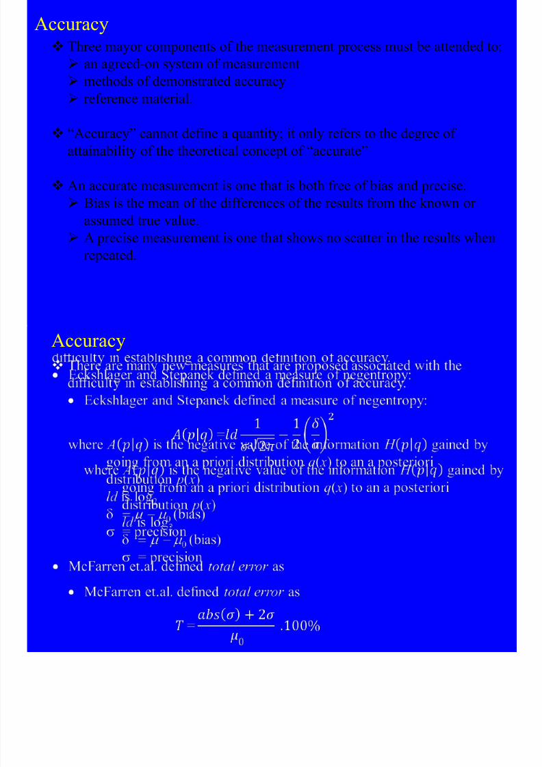
Accuracy Three mayor components of the measurement process must be attended t
an agreed-on system of measurement

8/10/2019 Kimia Analitik Lanjut
http://slidepdf.com/reader/full/kimia-analitik-lanjut 90/270
methods of demonstrated accuracy
reference material.
“Accuracy” cannot define a quantity; it only refers to the degree ofattainability of the theoretical concept of “accurate”
An accurate measurement is one that is both free of bias and precise. Bias is the mean of the differences of the results from the known or
assumed true value.
A precise measurement is one that shows no scatter in the results when
repeated.

8/10/2019 Kimia Analitik Lanjut
http://slidepdf.com/reader/full/kimia-analitik-lanjut 91/270
AccuracyA method with a total error less than 25% is qualified as excellent; 25 – 50% is considered acceptable.

8/10/2019 Kimia Analitik Lanjut
http://slidepdf.com/reader/full/kimia-analitik-lanjut 92/270
Wolter et.al. defined the maximum total error, the maximum differenc
between a measured value and the true value that can occur with a probability of 95%:
where MTE(u) = upper limit maximum total error
RE(u) = upper limit random error, comprising the c2 distribution
SE(u) or SE(l ) = upper (lower) limit of the systemic error
MTE(u) = RE(u) + max{abs[SE(u)], abs[SE(l )]}

8/10/2019 Kimia Analitik Lanjut
http://slidepdf.com/reader/full/kimia-analitik-lanjut 93/270
Accuracy Secondary standards.
Measurement by two or more independent and reliable methods whos
estimated inaccuracies are small relative to accuracy required for

8/10/2019 Kimia Analitik Lanjut
http://slidepdf.com/reader/full/kimia-analitik-lanjut 94/270
estimated inaccuracies are small, relative to accuracy required for
certification.
Measurement via a qualified network of laboratories.
Standard methods.
The composition on the material to be known can be obtained by applyin
an agreed-on method of analysis, for instance, a method issued by the
International Standard Organization (ISO) and the American Society ofTesting Materials (ASTM). The value obtained by analysis according to a
standard method can be assumed to be a “true value‟. This method ofensuring accuracy is often used in trade.
Mean is true. The mean of the results of a number of independent selecte
laboratories can be assumed to be the “true value”
AccuracyWhen the degree of accuracy is estimated, two related questions are often
encountered:
1 When is the bias significant or what is the probability that a found bi
8/10/2019 Kimia Analitik Lanjut
http://slidepdf.com/reader/full/kimia-analitik-lanjut 95/270
1. When is the bias significant, or what is the probability that a found bi
is real?
2. How can bias be distinguished from random error? (it is dealt with inthe discussions of analysis of variance and sequential analysis).
It should be stressed that random errors may seem to be bias, in particula
when the random errors is large compared to the bias. If a sample that too
small is taken from an inhomogeneous object, the result of the analysis mdeviate appreciably from the results of a thoroughly mixed standard.
Repeating the analysis with a standard method may indicate that no real b
is present. Even when the analytical method shows no bias at all, the
method cannot be designated as accurate when the precision is insufficien
It is useless to look for an accurate method of analysis in situations where
sampling shows a bias or random error that is large compared to bias and
precision of the analysis method
Accuracy

8/10/2019 Kimia Analitik Lanjut
http://slidepdf.com/reader/full/kimia-analitik-lanjut 96/270
This method is based on the assumption that the mean value of a ser
of observation shows a distribution around the mean value estimatedfrom an infinitely large series, just as individual observations show a
distribution around their mean. The distribution of the means has a
probability density function that resembles the well-known Gaussian
distribution for individual observations. This distribution is called th
distribution.
Accuracy

8/10/2019 Kimia Analitik Lanjut
http://slidepdf.com/reader/full/kimia-analitik-lanjut 97/270
Limit of Detection Whenever a sample containing a compound in a very low concentration h
to be measured by an analytical procedure, the signal from the measuring
instrument as a rule will be small. It is difficult to decide whether the sign

8/10/2019 Kimia Analitik Lanjut
http://slidepdf.com/reader/full/kimia-analitik-lanjut 98/270
g
emerges from the component to be determined or from the inevitable noi
produced by the procedure or the instrument.
The uncertainty gives rise to the so-called limit of detection. The quality
this limit can be determined by statistical means.
When one is deciding whether a measured signal originates from themeasured property or does not, some incorrect decisions can be made:
A decision that the component was present in the sample when in fact
was not: error of the first kind.
A decision that the component was not present in the sample when in
it was: error of the second kind.

8/10/2019 Kimia Analitik Lanjut
http://slidepdf.com/reader/full/kimia-analitik-lanjut 99/270
Limit of Detection

8/10/2019 Kimia Analitik Lanjut
http://slidepdf.com/reader/full/kimia-analitik-lanjut 100/270
b
a
f( x)
x
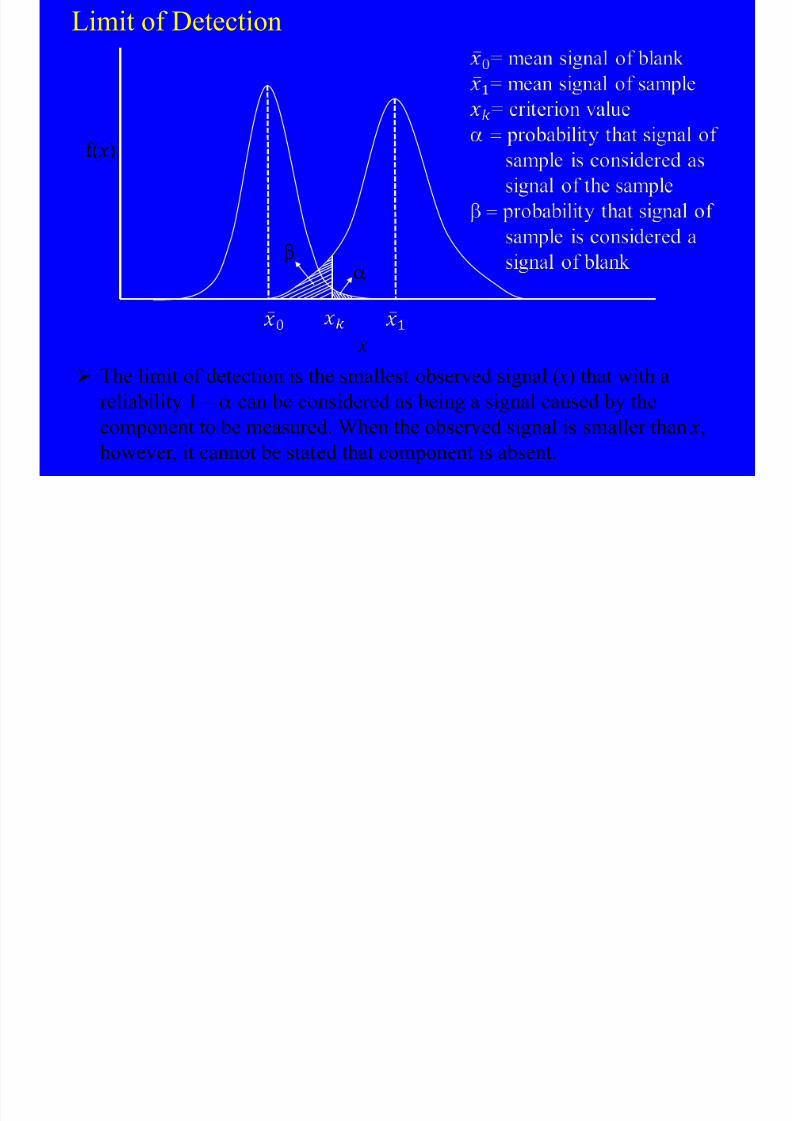
The limit of detection is the smallest observed signal ( x) that with a
reliability 1 – a can be considered as being a signal caused by thecomponent to be measured. When the observed signal is smaller than x,
however, it cannot be stated that component is absent.
Limit of Detection
8/10/2019 Kimia Analitik Lanjut
http://slidepdf.com/reader/full/kimia-analitik-lanjut 101/270
If the signal with magnitude xk is used as a criterion for the presence ofcomponent c, the probability a that an observed signal x > xk caused the
blank is
where P 0( x) = probability distribution of x0 P 1( x) = probability distribution of x1
The probability b that a signal will be observed that is less than xk and
caused by the sample (concentration component x1) is
Limit of Detection

8/10/2019 Kimia Analitik Lanjut
http://slidepdf.com/reader/full/kimia-analitik-lanjut 102/270
The composition derived from signal x is
where S = sensitivity
Limit of Detection The value of k can be obtained in various ways:
1. When the probability distribution x0 is known with sufficient confide
and proved to be Gaussian, a and k are related as shown in the Table

8/10/2019 Kimia Analitik Lanjut
http://slidepdf.com/reader/full/kimia-analitik-lanjut 103/270
An often used value of a = 0.0013 (1 – a = 99.87%) results in k = 3, that
Table Value of k
a k
0.5000 0
0.1587 1.0
0.0228 2.0
0.0062 2.50.0026 2.8
0.0013 3.0
0.0005 3.3
Limit of Detection2. When s is not known but estimated a s from finite number of
observations, Student‟s-t must be used (t is correction factor used to
compensate for the uncertainty in the estimation of s)

8/10/2019 Kimia Analitik Lanjut
http://slidepdf.com/reader/full/kimia-analitik-lanjut 104/270
When for a certain method of analysis the limit of detection x is set equal the mean of the blank signal,
then k = 0 and a = 0.5. This implies that a random result is obtained. The
probability that a signal of a concentration equal to the blank will beconsidered as a signal of the component is 50%. If the obtained signal x =
and k = 3,
b
Limit of Detection

8/10/2019 Kimia Analitik Lanjut
http://slidepdf.com/reader/full/kimia-analitik-lanjut 105/270
b
a
f( x)
x
The probability a that a signal caused by the blank will be considered as
signal caused by the component is 0.0013 (see the Figure) (assuming
s0 = s1); b, the probability that a signal caused by component will be
considered to be caused by the blank, is now 50%.
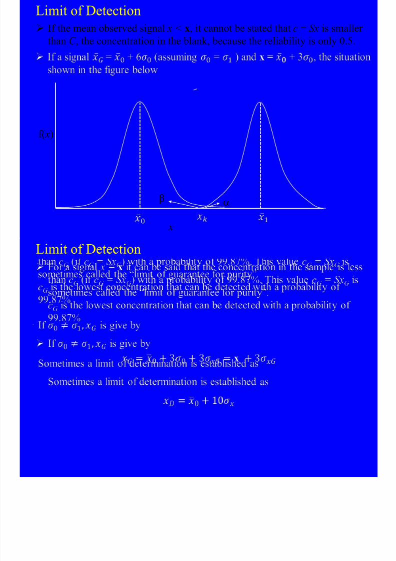
Limit of Detection If the mean observed signal x < x, it cannot be stated that c = Sx is smalle
than C , the concentration in the blank, because the reliability is only 0.5.

8/10/2019 Kimia Analitik Lanjut
http://slidepdf.com/reader/full/kimia-analitik-lanjut 106/270
ba
f( x)
x
Limit of Detection

8/10/2019 Kimia Analitik Lanjut
http://slidepdf.com/reader/full/kimia-analitik-lanjut 107/270
Limit of Detection

8/10/2019 Kimia Analitik Lanjut
http://slidepdf.com/reader/full/kimia-analitik-lanjut 108/270
x x
I II III
Three area according Currie:
Limit of Detection

8/10/2019 Kimia Analitik Lanjut
http://slidepdf.com/reader/full/kimia-analitik-lanjut 109/270
This procedure is applied for enhancing signal-to-noise ratios at the expe
of analysis time
Limit of Detection
8/10/2019 Kimia Analitik Lanjut
http://slidepdf.com/reader/full/kimia-analitik-lanjut 110/270
Limit of Detection For skewed data a transformation can be obligatory. In gamma spectrome
x-ray spectrometry, and other analytical methods based on particle/radiati
counting, the limit of detection depends more on the counting time than o

8/10/2019 Kimia Analitik Lanjut
http://slidepdf.com/reader/full/kimia-analitik-lanjut 111/270
the background and blank values.
Sensitivity Sensitivity is the ratio of the quantitative output and the input, for a given
qualitative range. For example S (l = 534 nm) = y/x, where y = extinction
534 nm; x = concentration of component x.

8/10/2019 Kimia Analitik Lanjut
http://slidepdf.com/reader/full/kimia-analitik-lanjut 112/270
Often, however, y is composed of a part that depends on x and a partindependent of x (blank). As a rule y is not linearly proportional to x over
entire range of possible x and y values.
The range for which S exists and has an unambiguous value is the dynamrange of the procedure.
Mostly for reasons of convenience, it is developed an analytical method i
which S has a constant value in a range as large as possible. The range is
called the linear dynamic range and is expressed in the orders of magnitufor which s can be considered to be constant.
Sensitivity The dynamic range is limited at the lower level by the value of x where y
cannot be distinguished from the noise in y. Here S may have all possible
values.
8/10/2019 Kimia Analitik Lanjut
http://slidepdf.com/reader/full/kimia-analitik-lanjut 113/270
blank
x
linear dynamic range
Sensitivity In situation where the analytical procedure consists of a chain of procedu
the sensitivity S can be subdivided into sensitivities belonging to the
consecutive operations:

8/10/2019 Kimia Analitik Lanjut
http://slidepdf.com/reader/full/kimia-analitik-lanjut 114/270
S 1 S 1 S 1 S 1 x x1 x2 x3 xn
y1 y2 y3 yn
y
Cumulative sensitivity for a signal y resulting from a number of consecutiv
operation S i on an input signal x.
Sensitivity The dimension of S depends on the dimension of x and y. If, for example,
is given in grams and y in milliamperes, the sensitivity S is expressed in
mA/g.

8/10/2019 Kimia Analitik Lanjut
http://slidepdf.com/reader/full/kimia-analitik-lanjut 115/270
Consider the chain of procedures: Concentration (g/L) converted into a potential (mV): S = mV/(g/L)
Potential converted into deflection of a recorder pen (cm): S = cm/mV
Then the ultimate sensitivity is expressed in
The foregoing holds only for static measurements. Under dynamic
circumstances S is time dependent. A sudden disturbance of the value of x
not momentarily followed by an output y; dy/dx is a fuction of t.
Sensitivity If we assume that y is related to x according to a first-order differential
equation, a stepwise disturbance of 0 → x results in

8/10/2019 Kimia Analitik Lanjut
http://slidepdf.com/reader/full/kimia-analitik-lanjut 116/270
where T x = time constant of procedureBecause the output y is time dependent. There will be a bias between
y(t→∞) = Sx and
x'Sx'
t tm t
y x
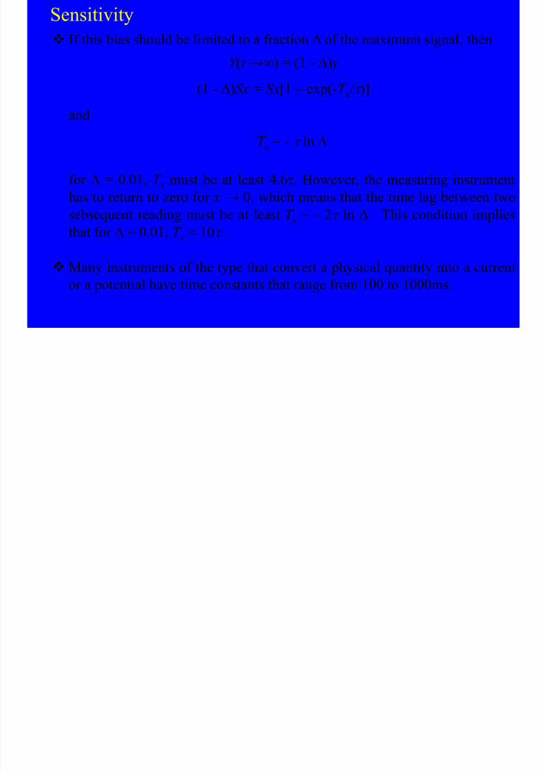
Sensitivity If this bias should be limited to a fraction ∆ of the maximum signal, then
Y (t →∞) = (1 - ∆) y
(1 - ∆)Sx = Sx[1 – exp(-T x / t )]

8/10/2019 Kimia Analitik Lanjut
http://slidepdf.com/reader/full/kimia-analitik-lanjut 117/270
( ) [ p( x )]
and
T x = - t ln ∆
for ∆ = 0.01, T x must be at least 4.6t. However, the measuring instrum
has to return to zero for x → 0, which means that the time lag between sebsequent reading must be at least T x = - 2t ln ∆. This condition imp
that for ∆ = 0.01, T x ≈ 10t .
Many instruments of the type that convert a physical quantity into a curr
or a potential have time constants that range from 100 to 1000ms.
Controllability and Measurability
In studying processes one is interested in an estimation of the quality of
equipment and procedures that are applied for measurement and for proce
control. Criteria that may allow an estimation of this quality are
measurability and controllability

8/10/2019 Kimia Analitik Lanjut
http://slidepdf.com/reader/full/kimia-analitik-lanjut 118/270
measurability and controllability.
The purpose of control is to diminish the variance of the process. The
parameter that describes the success or the maximum available success of
controlling action is based on diminution of the variance. The controllabi
factor is defined as
A factor r = 1 means that the variations in the process are fully eliminatedand control is 100% successful. A factor r = 0 means that no diminution a
all occurred.
Controllability and Measurability The controllability is determined by several factors, some related to the
control mechanism, others related to the measuring device applied, and al
related to the process to be controlled.

8/10/2019 Kimia Analitik Lanjut
http://slidepdf.com/reader/full/kimia-analitik-lanjut 119/270
The controllability factor can be divided into two parts: r p is related to control
m is related to measurement
For the purpose of sampling, only m is of interest.
The measurability factor m describes the influence of the measuring devicon control. When the control action is perfect, r p =1; in such a situation it
can be shown that m determines the maximum obtainable value of r :
where m D = e-d (measurability caused by delay time of analysis)
m A = e-a/2
(measurability caused by sampling frequency A-1
)mG = e-g/ 3 (measurability caused by sample size)
m N = 1 – sat e1/2 (measurability caused by precision of analysis)
Controllability and Measurability
or
From this equation it follows that the sample size should be kept to a
minimum.

8/10/2019 Kimia Analitik Lanjut
http://slidepdf.com/reader/full/kimia-analitik-lanjut 120/270
In order to describe the influence of sampling it can be stated that
Controllability and Measurability
The controllability is given by the numerical reduction of the value of a
disturbance of the process s x by a controlling action. The remaining value
the disturbance after control, s, and that before define the controllability
factor r according to

8/10/2019 Kimia Analitik Lanjut
http://slidepdf.com/reader/full/kimia-analitik-lanjut 121/270
g

8/10/2019 Kimia Analitik Lanjut
http://slidepdf.com/reader/full/kimia-analitik-lanjut 122/270
Controllability and Measurability
The frequency of the process fluctuations follows from autocorrelation
function of xt . The autocorrelation gives a relationship between a process
value of time t and that of another time. This predicting element can be us
for measurability and controllability.

8/10/2019 Kimia Analitik Lanjut
http://slidepdf.com/reader/full/kimia-analitik-lanjut 123/270
When the result of a measurement has been obtained, a prediction can be
made of the value of x in the future, a period t later. The uncertainty in th
prediction is given by the predicted variance
Controllability and Measurability

8/10/2019 Kimia Analitik Lanjut
http://slidepdf.com/reader/full/kimia-analitik-lanjut 124/270
Controllability and Measurability

8/10/2019 Kimia Analitik Lanjut
http://slidepdf.com/reader/full/kimia-analitik-lanjut 125/270
When the accuracy s a of the measuring method and the sample size T g is
included:
Or, for short,
Controllability and MeasurabilityTable Reduction of Disturbances
s min / s x m
0.10 0.995

8/10/2019 Kimia Analitik Lanjut
http://slidepdf.com/reader/full/kimia-analitik-lanjut 126/270
0.25 0.970.50 0.87
0.87 0.5
In situations encountered in practice it is hardly a disadvantage because lo
m imply (1 – m2
)1/2
≈ 1, so the variance decrease is negligible and thusimmaterial that m may have an approximated value.
Controllability and Measurability Example: the analysis of the nitrogen content of fertilizer. There are many
methods available to do this analysis. These method are compared on the
basis of measurability factors.
The production of fertilizer in a continuous process sets the following

8/10/2019 Kimia Analitik Lanjut
http://slidepdf.com/reader/full/kimia-analitik-lanjut 127/270
The production of fertilizer in a continuous process sets the following
numerical values:
T a = 30 minutes s x = 1.2% nitrogen
T x = 66 minutes ma = 0.80%
The methods of analysis are listed in the Table below
Table Methods for Analysis of Nitrogen in Fertilizer *
Dead Time SD
Criterion and of Analysis of Analysis
Analytical Techniques (minutes) (%N) (md )a mn m
Total N, classical
distillation 75 0.17 0.32 0.99 0

8/10/2019 Kimia Analitik Lanjut
http://slidepdf.com/reader/full/kimia-analitik-lanjut 128/270
Total N, DSMAutomated analyzer 12 0.25 0.84 0.97 0
NO3-N, Technicon
Autoanalyzer 15.5 0.51 0.79 0.92 0
NO3-N, specific
electrode 10 0.76 0.86 0.85 0
NH4 NO3/CaCO3 ratio,X-ray diffraction 8 0.8 0.89 0.83 0
Total N, fast neutron
Activation analysis 5 0.17 0.93 0.99 0
Specific gravity, g-ray
absorption 1 0.64 0.98 0.88 0
* A sampling frequency of 2 samples/hour is assumed, which means that ma = 0.80; (md )a =
measurability caused by analysis time; mn = measurability caused by accuracy.
Controllability and Measurability
It is seen that the highest m value is given by neutron activation. In a
practical situation the cost of the equipment can play an important role in
solution of a particular procedure. In static situations the analysis time
becomes unimportant.

8/10/2019 Kimia Analitik Lanjut
http://slidepdf.com/reader/full/kimia-analitik-lanjut 129/270
Here the specific gravity measurement by g-ray absorption, a very inaccu
method, gives the second-best results concerning information and is much
cheaper than neutron-activation method. When it is taken into account tha
the g-ray absorption method can be repeated after 1 minute, (T a = 1 minut
then for this method mtotal = 0.86, by far the best method.
Measuring Functions and Calibration Functions
During the analysis of a sample, a number of actions are performed,
resulting in one or more measured data that are used to calculate quantitat
analytical results.

8/10/2019 Kimia Analitik Lanjut
http://slidepdf.com/reader/full/kimia-analitik-lanjut 130/270
Analysis may be considered to be a process with input parameters oncomposition, denoted as concentrations xi and with output parameters
measured data yi:
xi PROCEDURE yi
where i = 1,2,3, ……, n j = 1,2,3, …...., m
In order to evaluate from yi the value for xi, the functional relationship
between yi and xi should be known. The establishment of this functional
relationship is called calibration. An analytical method for analysis of n compounds x1, x2,……. xn of a
sample should produce y1, y2,……. yn measured data (m ≥ n).
Measuring Functions and Calibration Functions
The functional relationship between measured data y and composition x is
called the calibration function.
In order to apply a given analytical procedure for chemical analysis, each

8/10/2019 Kimia Analitik Lanjut
http://slidepdf.com/reader/full/kimia-analitik-lanjut 131/270
measurement y j should correspond to a composition xi according to xi = y j ( y j, all x except xi)
This condition implies that in order to measure one concentration value xi, a
other n concentrations x j ( j ≠ i) should be known, or that these values shoul
measured by collecting at least n – 1 more yi values.
For quantitative analysis the solution of m equations with n unknowns (m ≥
x1 = g 1 ( y1, y2,……. ym)
x2 = g 2 ( y1, y2,……. ym)
.
.
xn = g n ( y1, y2,……. ym)

8/10/2019 Kimia Analitik Lanjut
http://slidepdf.com/reader/full/kimia-analitik-lanjut 132/270
Measuring Functions and Calibration Functions
As a rule of thumb, one may state that the resulting n·n matrix should be su
that its determinant has a maximal value. This means that the determinant h
highest possible elements on the diagonal and smallest possible elements on
the nondiagonal positions. A generally accepted method to reduce the numb

8/10/2019 Kimia Analitik Lanjut
http://slidepdf.com/reader/full/kimia-analitik-lanjut 133/270
of column is to multiply the matrices with their transpose.Example: in a spectrophotometric measurement on chlorine and bromine
dissolved in a suitable solvent, extinction coefficients a x are known. In a mixtu
of Cl2 and Br 2, the measurement results of log (I0/I)l with optical path length 1
cm are as follows:
l (nm) aCl2 (1/mol cm) aBrl2 (1/mol cm) log (I0/I)l = y y
455 4.5 168 0.1995
417 8.4 211 0.2698
385 20 158 0.2980
357 56 30 0.4220333 100 4.7 0.7047
312 71 5.3 0.5023
Measuring Functions and Calibration Functions
at ·yl = at ·a·x·d

8/10/2019 Kimia Analitik Lanjut
http://slidepdf.com/reader/full/kimia-analitik-lanjut 134/270
which become
Measuring Functions and Calibration Functions
It is seen that the determinant F is well conditioned because
8214.7 < 18667.81 and < 98659.18.
Application of Cramer‟s rule (provided det ≠ 0) gives

8/10/2019 Kimia Analitik Lanjut
http://slidepdf.com/reader/full/kimia-analitik-lanjut 135/270
Selectivity and Specificity
In quantitatively analysis the measurement of one particular component o
mixture may be disturbed by other components of the mixture. This mean
that the measurement is nonspecific for the compound under investigatio

8/10/2019 Kimia Analitik Lanjut
http://slidepdf.com/reader/full/kimia-analitik-lanjut 136/270
A completely specific method for a compound can measure the
concentration of that component, regardless of what other compounds are
present in the sample. The other components do not produce an analytica
signal.
A very important quality criterion of an analytical method is its capabilit
to deliver signals that are free from interferences and give “true results”.The ability to discriminate between the analyte and interfering componen
is expressed as the “selectivity” of a method and measurement system.
Selectivity and Specificity
A method of analysis is called completely selective when it produces corr
analytical results for various components of a mixture without any mutua
interaction of the components. A selective method thus is composed of a
series of specific measurements.

8/10/2019 Kimia Analitik Lanjut
http://slidepdf.com/reader/full/kimia-analitik-lanjut 137/270
“Selectivity of a method refers to the extent to which it can determine
particular analyte(s) in a complex mixture without interference from othe
components in the mixture”
The use of the term “selectivity” in analytical chemistry has evolved in
parallel with the development of more sensitive and discriminating methothat have a capability to identify and quantify analytes with less interfere
from other components, similar or dissimilar, than earlier methods were a
to do.
Modern methods are usually designed by combining several measuremen principles introducing their own selectivity to the overall operation. In th
way, very highly selective methods can be obtained.
Selectivity and Specificity
In situation where the linear system holds,
y = F x
the measurement for component k is specific when only the terms f i

8/10/2019 Kimia Analitik Lanjut
http://slidepdf.com/reader/full/kimia-analitik-lanjut 138/270
=1,…, n) are non-zero. Here the matrix is called F spec and the value of yfunction of xk only.
For completely selective method each row of matrix F contains only
nonzero element. By interchanging rows, one may get a matrix F , ca
F sel, with all nonzero elements on the diagonal.
In practical situations F sel and F spec contaion other nonzero elements. Th
elements, however, have considerably smaller values than the correspond
f i,k values.
The undesired nonzero elements of F sel and F spec can be used fo
quantitative description of selectivity and specificity.

8/10/2019 Kimia Analitik Lanjut
http://slidepdf.com/reader/full/kimia-analitik-lanjut 139/270
The Ruggedness Test
Precision involves the determination of the random error under specific
circumstances.
The level at which a method has to be tested depends on its later use.

8/10/2019 Kimia Analitik Lanjut
http://slidepdf.com/reader/full/kimia-analitik-lanjut 140/270
Whenever an analytical method has to be applied in different site or
laboratories, eventually an interlaboratory test must be carried out to ensu
that the method performs adequately in different circumstances.
The variability of a method under identical circumstances, e.g., in thedeveloper laboratory, is called the repeatability, whereas the precision in
different circumstances is called the reproducibility..
An interlaboratory study can be very costly and should only be undertake
when there is a reasonable chance that a method will be accepted.

8/10/2019 Kimia Analitik Lanjut
http://slidepdf.com/reader/full/kimia-analitik-lanjut 141/270

8/10/2019 Kimia Analitik Lanjut
http://slidepdf.com/reader/full/kimia-analitik-lanjut 142/270
The Ruggedness Test
Example of Possible Critical Factors and Levels for HPLC Experiments
Critical Factor Deviation from Nominal Value
Sample preparation factors:
Sample weight 1%

8/10/2019 Kimia Analitik Lanjut
http://slidepdf.com/reader/full/kimia-analitik-lanjut 143/270
Shake time 20%Sonicate time 20%
Heating temperature 5 0C
Wash volume 30%
Extraction volume 30%
Centrifuge time 20%
Pore size of filter 5 mm⁞
Chromatographic factors
pH 1
Temperature 5 0C
Solvent % 3%
Flow rate 0.1 mL/ minBuffer concentration 1%
Additive concentration 0.5%
The Ruggedness Test
Example of Possible Critical Factors and Levels for HPLC Experiments
Critical Factor Deviation from Nominal Value
Column factors:
Manufacture
B h

8/10/2019 Kimia Analitik Lanjut
http://slidepdf.com/reader/full/kimia-analitik-lanjut 144/270
Batch⁞
Detector factors
Wavelength 5 nm
Time constant 5
⁞
The Ruggedness Test
The number of factors that have to be tested is usually large. Even when
only the most important factors are selected, a large number of experimen
are necessary. The basic idea is not to change one factor at a time but rath
simultaneously to change several factors in such a way that it is possible
identify the changes that produce an influence on the method‟s performan

8/10/2019 Kimia Analitik Lanjut
http://slidepdf.com/reader/full/kimia-analitik-lanjut 145/270
Factorial designs are the most suitable for ruggedness testing. They enab
one to establish the influence of each of the factors separately (main effec
and the interactions between them. The number of experiments required i
2
n
, n being the number of factors to be tested. For 7 factors this means 2128 experiments.
In practice full factorial designs can only be used when the number of
factors to be used is low. When it can be assumed that there are no
significant higher order interactions between the factors, which is often arealistic assumption, the fractional factorial designs are most efficient.
Saturated fractional factorial designs enable one to test N – 1 factors with
experiments.
An example of a Placket-Burman design for 12 experiments to test a
i 11 f t Wh th iti l f t id tifi d d th
The Ruggedness Test

8/10/2019 Kimia Analitik Lanjut
http://slidepdf.com/reader/full/kimia-analitik-lanjut 146/270
maximum 11 factors. When the critical factors are identified and theexperimental design is selected, the experimental work can be carried ou
This involves performing the experiments prescribed by the experimenta
design.
To avoid artifacts, it is necessary to perform these experiment in a randomsequence. The performance of the methods for the different experiments
must be recorded. For HPLC experiments several performance paramete
can be selected. The most relevant of these are the following: the
concentration calculated from the peak height or peak area; the retention
time; the resolution, etc.
Factors
Exp I II III IV V VI VII VIII IX X XI Res
1 76 76 -76 76 76 76 -76 -76 -76 76 -76 7
2 12 12 12 12 12 12 12 12 12 12 12
Placket – Burman Design

8/10/2019 Kimia Analitik Lanjut
http://slidepdf.com/reader/full/kimia-analitik-lanjut 147/270
Factor
2 12 -12 12 12 12 -12 -12 -12 12 -12 12 3 -21 21 21 21 -21 -21 -21 21 -21 21 21 2
4 25 25 25 -25 -25 -25 25 -25 25 25 -25 2
5 360 360 -360 -360 -360 360 360 360 360 -360 360 3
6 318 -318 -318 -318 318 -318 318 -318 318 318 318 3
7 -29 -29 -29 29 -29 29 -29 29 29 29 29 28 314 314 314 314 314 314 314 314 314 314 314 3
9 -50 50 -50 50 50 -50 50 50 50 -50 -50 5
10 25 -25 25 25 -25 25 25 25 25 -25 -25 2
11 -30 30 30 -30 30 30 30 -30 -30 -30 30 3
12 -230 -230 -230 -230 -230 -230 -230 -230 -230 -230 -230 2
The Ruggedness Test
From the Table it can be seen that for the first factor the experiment 1, 2,
5, 6, and 10 involve the factor at the extreme level, whereas the experime
3, 7, 8, 9, 11, and 12 involve this factor at the nominal level. The main
effect of factor 1 is then calculated as

8/10/2019 Kimia Analitik Lanjut
http://slidepdf.com/reader/full/kimia-analitik-lanjut 148/270
If no factor has an influence, all the effects should be small and of abothe same size.
If one or two factors have an influence on the performance of the
method, then the values of their main effects will be much larger than
other main effects.
The Ruggedness Test
Obviously a method should not be influenced by the small variations
introduced for the ruggedness test that are expected to be encountered in
practice.
If there are no large difference, the analytical error can be estimated from
h f h i ff

8/10/2019 Kimia Analitik Lanjut
http://slidepdf.com/reader/full/kimia-analitik-lanjut 149/270
the mean of the main effects:
The estimate of standard deviation reflects the differences that have been
created to simulate the situation that different laboratories have been
carrying out the experiments. If this standard deviation is unsatisfactorily
high, then a interlaboratory test will certainly yield unsatisfactorily result
The Ruggedness Test
If one or two factors show an important influence on the method‟s performance, then the method should be improved to make it more rugge
to the small variations in these factors.
When this is not possible then the method procedure should specify a str
8/10/2019 Kimia Analitik Lanjut
http://slidepdf.com/reader/full/kimia-analitik-lanjut 150/270
When this is not possible, then the method procedure should specify a strrange these factors, which is chosen so that the performance is adequate
when the factor remain in that interval.
Structure of an expert system for ruggedness analysis
Supervisor
Supervisor
Frame

8/10/2019 Kimia Analitik Lanjut
http://slidepdf.com/reader/full/kimia-analitik-lanjut 151/270
Factor
Choice
Design
selection
Statistical
results
Chemical
results
Method
improv-
ement
Reselec
factor
levels
Common Data Structure
Explain
Control Chart One of the oldest methods used to monitor and control quality of a
procedure, -in particular, the accuracy and precision- is control chart.
A control chart is a graphic representation on which the values of the
quality characteristic under investigation are plotted sequentially.
l h b i l li d id hi

8/10/2019 Kimia Analitik Lanjut
http://slidepdf.com/reader/full/kimia-analitik-lanjut 152/270
Control charts are basic tools for quality assurance and provide a graphic
means to demonstrate statistical control, monitor a measurement process
diagnose measurement problem, document measurement uncertainty, and
generally aid in methodology development.
Control charts may also be used to monitor and/or document critical aspe
of samples and sampling operations.
Control Chart

8/10/2019 Kimia Analitik Lanjut
http://slidepdf.com/reader/full/kimia-analitik-lanjut 153/270

8/10/2019 Kimia Analitik Lanjut
http://slidepdf.com/reader/full/kimia-analitik-lanjut 154/270
Control Chart Limits are indicated within which the plotted values may be expected to
while the process is in a state of statistical control.
The limits in the X chart are simply “3-sigma” limits, following the origi
Shewart format that indicate the bounds within which substantially all oth d t h ld li h th t i i t t f t ti ti l t l

8/10/2019 Kimia Analitik Lanjut
http://slidepdf.com/reader/full/kimia-analitik-lanjut 155/270
Shewart format, that indicate the bounds within which substantially all othe data should lie when the system is in a state of statistical control.
An chart is preferable because it is less sensitive to blunders (occasion
wild results), but such charts may not be feasible for the time-consumin
requirements that are the hallmarks of analytical chemistry. Another reasfor preference is that means are more likely to be normally distributed th
individual values, which is important because a normal distribution is
ordinarily assumed when setting control limits.
While an X chart has the advantage of requiring less work, additionalmeasurements may be required on occasion to confirm an apparent
indication of “out of control”.
Control Chart A precision chart consists of standard deviation (for the range which is
related to), evaluated at various times, plotted in a fashion similar to the
above. Ordinarily, several (at least 4) measurements are needed to evalua
the standard deviation on each occasion, and this requirement is its mayo
disadvantage The range chart is a useful type of precision chart

8/10/2019 Kimia Analitik Lanjut
http://slidepdf.com/reader/full/kimia-analitik-lanjut 156/270
disadvantage. The range chart is a useful type of precision chart.
The maintenance of property charts and precision charts in parallel has
considerable diagnostic value. By inter-comparison of the charts, one can
usually determine whether bias, imprecision, or both are affecting a
measurement process.
Control Limits Control limits can be based on established limits or experimentally
established ones. For manufactured goods, the limits could be based on
acceptability product with the central line as a desired value and the cont
limits as permissible tolerances.
Similarly in measurement the certified value of a control sample could
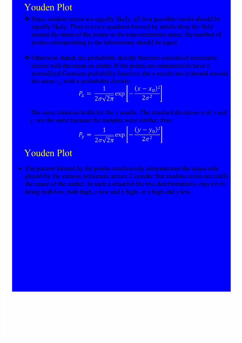
8/10/2019 Kimia Analitik Lanjut
http://slidepdf.com/reader/full/kimia-analitik-lanjut 157/270
Similarly, in measurement, the certified value of a control sample couldserve as the central line while the limits could reflect a permissible
uncertainty for the measurement process.
The above approach is no longer considered favorably, since it does not
really monitor either a production process or a measurement process, butmerely indicates what can be gotten away with.
The recommended procedure, almost universally followed today, uses th
means of a number of measured values of the variable as the central line
and the experimentally estimated standard deviation to establish the contand warning limits.

8/10/2019 Kimia Analitik Lanjut
http://slidepdf.com/reader/full/kimia-analitik-lanjut 158/270
Control Samples The control sample must have a high degree of similarity to the actual
samples analyzed. Otherwise, one cannot draw reliable conclusions the
performance of the measurement system on test samples from its
measurement of control samples.
The control samples must be sufficiently homogenous and stable so the

8/10/2019 Kimia Analitik Lanjut
http://slidepdf.com/reader/full/kimia-analitik-lanjut 159/270
The control samples must be sufficiently homogenous and stable so theindividual increments measured at various times will have less variability
than of the measurement process.
When the value of the property measured is known with sufficient accur
both the precision of measurement and any systematic measurement erro(bias) can be estimated. Even, if the exact composition is not known, a
suitable control sample can evaluate the stability and precision of the
measurement process.
Ideally, a control chart should bet that is me established for each kind
measurement that is made, and indeed, for each parameter level as well.
Frequency of Control Measurements The required frequency of measurement of control samples will depend o
• the known stability of measurement process
• The importance of the decisions based on the measurement data . Cont
intervals should be chosen with realization that any data obtained durin
the period from last-known-in-control to first-known-out-of-control wi
be in jeopardy

8/10/2019 Kimia Analitik Lanjut
http://slidepdf.com/reader/full/kimia-analitik-lanjut 160/270
be in jeopardy.
• The cost in time and effort of measuring a control sample. If this is
relatively small, one is well-advised to err on the conservative side and
measure more controls than the minimum number.
Guidance in choosing control sample intervals can be found by applying
“length of run” concept. The interval between retoolings in a production
process may be considered as a production run. Measurement systems m
be studied for possible runs, such as: between calibration, between days,
between shift, between rest periods, between periods of use, betweencritical adjustments.
Range Control Chart
The problem of appropriateness of control samples can be circumvented
using replicate measurements of the actual test samples to monitor
measurement precision.
A special case is the duplicate measurement of a reasonable number o
test samples. It will be remembered that the range of a set of

8/10/2019 Kimia Analitik Lanjut
http://slidepdf.com/reader/full/kimia-analitik-lanjut 161/270
p gmeasurements (in this case, the difference of the duplicate
measurements) is related to the standard deviation. Accordingly, range
control charts can be developed and used to monitor measurement
precision.
The range control charts do not evaluate systematic departures that woul
affect each measurement in the same way. Thus instrumental shifts and
calibration drifts would go undetected. It be needed to include other cont
samples and/or calibration checks to monitor such problems.
Range Control Chart The average value of the range is calculated from k sets of duplicate
measurements by the expression:
is the central line and the control limits are of using the factors foui h i i l bl h i l l f h f d d

8/10/2019 Kimia Analitik Lanjut
http://slidepdf.com/reader/full/kimia-analitik-lanjut 162/270
gin the statistical tables. The numerical value for the factor depends on
the number of measurements in the set, and the confidence level for
judgment of control.
Table Factors for use in Duplicate Range Charts and Other Sets of Replicates
Number in Set UWL UCL LCL
2 2.512 3.267 0
3 2.050 2.575 0
4 1.855 2.282 0
5 1.743 2.115 0
6 1.669 2.004 0
Use of Range Control Charts Duplicate measurements may be made of all samples measured, of select
samples in a measurement series of reference materials, or any
combination of the above as designated in the laboratory‟s qualityassurance program.
When the values of R are plotted on the chart, the following courses of
action are recommended:

8/10/2019 Kimia Analitik Lanjut
http://slidepdf.com/reader/full/kimia-analitik-lanjut 163/270
1. If R is within the warning limit, accept all related data.
2. If R is outside the control limits (UCL), the system is out-of-control.
Reject all data since last-known-to-be-in-control and take corrective
action.
3. If R exceeds the UWL but is within the UCL, accept measurements,tentatively. If the R for the next sample is within the UWL, accept al
the previous data. If it exceeds the UWL, reject all data taken since th
system was last-known-to-be-in control and take corrective actions.
Reestablish control before accepting data.
4. Reestablishment of control should be demonstrated by the results ofthree consecutive sets of measurement that are in control.
Cusum Charts The charts for average and range can be used when sudden changes shou
be detected. The chart is called as the cusum chart for controlling the
quality of analytical methods, whens sudden changes in the method,
application of wrong procedures, interchange of reagents, and the
breakdown of parts of instruments have to be detected.

8/10/2019 Kimia Analitik Lanjut
http://slidepdf.com/reader/full/kimia-analitik-lanjut 164/270
When more gradual changes should be detected, such as aging of reagen
and obsoleteness of standard curves, another method of plotting the resu
should be used.
The decision is based on the whole of the recent sequence of measureme
Instead of plotting the subgroup averages , a reference value k
chosen and the cumulative sum is calculated:
Cusum Charts Each sums, is obtained from its predecessor by the operation of adding th
new difference; k is a reference value that is chosen equal to the average
but calculation of the cumulative sums (abbreviated to cusum) is simplif
if a rounded value is chosen.
If the mean value of the subgroup averages remains close to the referencl f h diff i i d i h h

8/10/2019 Kimia Analitik Lanjut
http://slidepdf.com/reader/full/kimia-analitik-lanjut 165/270
value, some of the differences are positive and some negative, so that the
cusum chart is essentially horizontal. However, if the average value of th
process rises to a new constant level, more of the differences become
positive and the mean path slopes upward.
The position of the change in the cusum slope indicates the moment the
change in the quality parameter occurred. However, the visual picture
depends to some extend on the scales chosen for the axes of the chart. If
horizontal distance between the plotted points is regarded as one unit, it i
recommended that the same distance on the vertical scale representapproximately 2s /√n (s is the population standard deviation)
Youden Plot Youden plot method is the round-robin test with graphic reporting that is a
very popular and effective controlling device for analytical laboratories.
In experimental methodology, a round robin test is an interlaboratory te
(measurement, analysis, or experiment) performed independently severa
times. This can involve multiple independent scientists performing the te
with the use of the same method in different equipment, or a variety of

8/10/2019 Kimia Analitik Lanjut
http://slidepdf.com/reader/full/kimia-analitik-lanjut 166/270
methods and equipment. In reality it is often a combination of the two, f
example if a sample is analysed, or one (or more) of its properties is
measured by different laboratories using different methods, or even just
different units of equipment of identical construction.
A round robin program is a Measurement Systems Analysis techniquewhich uses Analysis of Variance (ANOVA) random effects model to ass
a measurement system.
The Youden plot is a graphical method to analyse inter-laboratory data,
where all laboratories have analysed 2 samples. The plot visualises with
laboratory variability as well as between-laboratory variability
Youden Plot

8/10/2019 Kimia Analitik Lanjut
http://slidepdf.com/reader/full/kimia-analitik-lanjut 167/270
The original youden plot. PR_A and PR_B
represent similar samples. Notice the two
outliers in the upper right corner of the graph.Circle represents 95% coverage probability
Example of a Youden plot adapted
samples that are not similar. Circle
represents 95% coverage probabilit
A 45-degree reference line is drawn through the Manhattan median
Points that lie near the 45-degree reference line but far from the Manhattan
median, indicate large systematic error.
Points that lie far from the 45-degree line indicate large random error.
Points outside the circle indicate large total error.
Youden Plot Since random errors are equally likely, all four possible results should be
equally likely. Thus in every quadrant formed by subdividing the field
around the mean of the points in the representations space, the number o
points corresponding to the laboratories should be equal.
Otherwise stated, the probability density function consists of concentric

8/10/2019 Kimia Analitik Lanjut
http://slidepdf.com/reader/full/kimia-analitik-lanjut 168/270
p y y
circles with the mean as center. If the points are considered to have a
normalized Gaussian probability function, the x results are scattered arou
the mean xo with a probability density
The same situation holds for the y results. The standard deviation s of x a
y are the same because the samples were similar; thus
Youden Plot
The pattern formed by the points conclusively demonstrates the major role
played by the various systematic errors. Consider that random errors are re
the cause of the scatter. In such a situation the two determinations, may err
being both low, both high, x low and y high, or x high and y low.

8/10/2019 Kimia Analitik Lanjut
http://slidepdf.com/reader/full/kimia-analitik-lanjut 169/270

8/10/2019 Kimia Analitik Lanjut
http://slidepdf.com/reader/full/kimia-analitik-lanjut 170/270
Youden Plot The same statement holds for low results. The elongation of the ellipse is
measure for the accuracy of the method, scales along the x- and y-axes
being the same. The distance of each point along the 45o axis to the mean
a measure of the systematic error that the laboratory is likely to have bee
making.
A laboratory that has large systems0

8/10/2019 Kimia Analitik Lanjut
http://slidepdf.com/reader/full/kimia-analitik-lanjut 171/270
errors will be represented by a poi
x, y in the Youden plot that sticks t
the 45o axis but the lies quite a
distance from x0
, y0
.
The distance of the point T( x1, y1)
the 45o axis is an estimate of the
random error (the precision) of thi
laboratory.
The distance from S to x0 , y
0 is an
estimate of the systematic error.
y
x
A
B
450
T b
d
S
x0y0
c
st
Youden Plot In fact the Youden plot is a graphic representation of an analysis of varian
The correlation between these methods can be seen by comparing some
parameters.
In an analysis variance the random error s 0 is estimated by

8/10/2019 Kimia Analitik Lanjut
http://slidepdf.com/reader/full/kimia-analitik-lanjut 172/270
where k = number of laboratory
n = number of analyses for each laboratory (here n = 2)
In the Youden plot (see Figure above)
Youden Plot

8/10/2019 Kimia Analitik Lanjut
http://slidepdf.com/reader/full/kimia-analitik-lanjut 173/270
In this case n = 2, so
In the analysis of variance the total error
Youden PlotWith n = 2
In the Youden plot,
h i ifi f h diff b l d i i b

8/10/2019 Kimia Analitik Lanjut
http://slidepdf.com/reader/full/kimia-analitik-lanjut 174/270
The significance of the difference between total error and precision s 0 can b
tested by applying the F -test:
For the value of F greater than the tabulated F (for reliability a, n1 = k-1 and
n2 = k-1) it may be supposed that a systematic error exists:
Youden Plot
The Youden plot can be used not only for comparison of the quality of
laboratories with regard to their results but also for comparison of the
quality of two methods of analysis with regard to their (in)sensitivity to
various laboratories.
In practice often only the qualitative result is presented in graphic form. I
h ld b d h hi k i ll b " li " i

8/10/2019 Kimia Analitik Lanjut
http://slidepdf.com/reader/full/kimia-analitik-lanjut 175/270
should be noted that this works quite well because "outliers," i.e.,
laboratories having points far from x0 , y0 along the 45o axis, seldom appe
at the same spot when the round-robin test is repeated.
It must be emphasized that quantitative results can be obtained only when
the distribution of the data is not significantly different from a normal one
For a skewed distribution, as may be the case when the samples x and y a
near the limit of detection, an appropriate linearizing methods should be
applied or the quantitative presentation should be abandoned in favor of t
graphic plot.
The Ranking Test
Another way to assess the quality of a laboratory or an analytical method
the application of the ranking test.
The laboratory's score equals the sum of the ranks it receives.

8/10/2019 Kimia Analitik Lanjut
http://slidepdf.com/reader/full/kimia-analitik-lanjut 176/270
The data from a collaborative test may be arranged in a classification
scheme as shown in Table below. The right-hand side of the table shows t
data substituted by rankings assigned to the laboratories according to the
measured concentration for a series of samples. Rank 1 is given to the
largest amount, rank 2 to the next largest, and so on.
When two laboratories have the same score for the xth place, each
laboratory is assigned the rank x + ½. For a triple tie for the xth place, all
three laboratories get the rank x + 1.
The Ranking Test
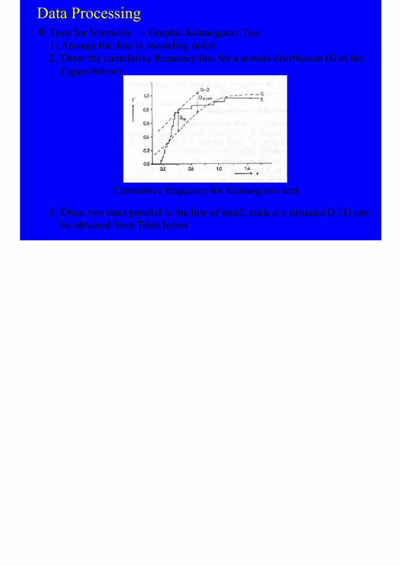
8/10/2019 Kimia Analitik Lanjut
http://slidepdf.com/reader/full/kimia-analitik-lanjut 177/270
The Ranking Test
For n samples, the minimum score is n and the maximum score is nm, whm denotes the number of participating laboratories.
A laboratory that scores the highest amount on every one of the n materia
gets the score of n.
Such a score is obviously associated with a laboratory that consistentlygets high results and the presumption is that this laboratory has a

8/10/2019 Kimia Analitik Lanjut
http://slidepdf.com/reader/full/kimia-analitik-lanjut 178/270
gets high results, and the presumption is that this laboratory has a
pronounced systematic error. When the results of the laboratories stem
from a random process, the scores tend to cluster around the value n(m
1)/2.
Sequential Analysis
Sequential analysis is a method used to guide statistical interference inobservation series in order to limit the number of observations of that seri
which is not known in advance.
When performing a series of experiments, one sometimes has to decide
whether the experiment gives a result that confirms the hypothesis that is
tested or whether alternatively this hypothesis must be rejected This test

8/10/2019 Kimia Analitik Lanjut
http://slidepdf.com/reader/full/kimia-analitik-lanjut 179/270
tested or whether, alternatively, this hypothesis must be rejected. This test
can be done by applying statistics to the set of observations.
There are then three possible decisions:
1. From the results obtained it is not yet possible to reject the hypothnor to accept it.
2. The hypothesis is rejected.
3. The hypothesis is acepted.
With the use of the proper statistics, decisions 2 and 3 can be made with
a certain degree of confidence.
Sequential Analysis
If decision 1 is the result, this means that the experiment has to be
continued. The question to be answered is now: how long should the
experiment be continued in order to reach decisions 2 or 3 with sufficient
but not too much- confidence?
By the sequential analysis method a test is conducted that allows a decisio
t b d ft h b ti Th th b b ti i

8/10/2019 Kimia Analitik Lanjut
http://slidepdf.com/reader/full/kimia-analitik-lanjut 180/270
to be made after each observation. Thus the number observations is
minimal.
Comparison of Sequential and Non-sequential Analyses
Sequential Analysis Non-sequential Analyses
The number of observations required is not The number of observation is known
known in advance. Before the experiment starts
After each observation one out of three After the experiment, comprising a se
possible decisions is selected: of observations, three decisions are1.Continue the experiment and make a new 1. Starts a new series of observations

8/10/2019 Kimia Analitik Lanjut
http://slidepdf.com/reader/full/kimia-analitik-lanjut 181/270
1.Continue the experiment and make a new 1. Starts a new series of observations
2.Reject the null hypothesis and terminate the 2. Reject the null hypothesis
experiment. 3. Accept the null hypothesis
3.Accept the null hypothesis and terminate the
experiment
After each observation the decision to terminate The experiment is terminated at the e
the experiment may result. of the series of observations.
The decision to terminate the experiment as a
rule results in fewer observations than in non-
sequential analysis.

8/10/2019 Kimia Analitik Lanjut
http://slidepdf.com/reader/full/kimia-analitik-lanjut 182/270
Sequential Analysis
Mathematical Description
Suppose a hypothesis H has to be tested by performing an experiment
that results in the variable x. Then x1 , x2 , …..xm are m observations of
variable x.
The progress of the test can be shown graphically by computing the
value of a function of all observations, F (m). This value is plotted as a
f nction of the n mber of obser ations

8/10/2019 Kimia Analitik Lanjut
http://slidepdf.com/reader/full/kimia-analitik-lanjut 183/270
function of the number of observations.
The sample space M m can be subdivided into three mutually exclusive
subspaces:
: space where H is accepted
: space where H is rejected
: space where no decision is possible
Sequential Analysis
Sequential analysis decision areas The direction of these boundar
depends on the values of a and
and the parameters tested (a:
probability of an error of the f
kind -reject H wrongly; b: probability of an error of the
III H0 accepted
R om

8/10/2019 Kimia Analitik Lanjut
http://slidepdf.com/reader/full/kimia-analitik-lanjut 184/270
f(m)
second kind -accept H wrongly
When the function value cross
one of the boundaries and entezone II or III, the experiment i
terminated by decision dictate
by the zone number.m
II H0 rejected
R m′
I no decision
R m
Data Processing
The first task of an analyst who analyze a process or procedure is to colle
relevant data of measurements on that process or procedure. The
information theory and the sampling strategy should be considered in
assuming what data are relevant and how many measurements
It also important to consider:
the reduction of the data collected according to a certain sampling

8/10/2019 Kimia Analitik Lanjut
http://slidepdf.com/reader/full/kimia-analitik-lanjut 185/270
the reduction of the data collected according to a certain sampling
strategy without loss of relevant information, and
the methods of data production
Data Processing
There are various methods of data production:
1. A measurement is made and the outcome of the measurement is foun
from the position of a dial on a scale of an instrument. It is the analy
who estimates the position of the dial and converts this to numbers in
digital notation.
2 The measurement is made continuously and translated in the position

8/10/2019 Kimia Analitik Lanjut
http://slidepdf.com/reader/full/kimia-analitik-lanjut 186/270
2. The measurement is made continuously and translated in the position
a recorder pen on a strip of recorder paper. The analyst reads the
position of the recorded pattern on the time base at times of interest a
converts the selected pen positions to digital numbers.
3. The measurement is made with a fixed frequency, converted
electronically in to a digital notation, and recorded on a device such
disk or magnetic tape. The analyst is not involved in this process, apa
from initiating the procedure of data collection.
Data Processing
The second task, after the numbers are obtained, is to reduce the number measurements, remove the erroneous and irrelevant data, and convert the
measurements in to statements pertaining to the condition of the process o
procedure under control.
In modern analytical procedures, a data acquisition rate of 105
measurements per second is not unusual. In order to convert this enormou

8/10/2019 Kimia Analitik Lanjut
http://slidepdf.com/reader/full/kimia-analitik-lanjut 187/270
measurements per second is not unusual. In order to convert this enormou
amount of data, collected, for example, during 7 day, into a form that can
handled, data reduction procedures should be applied. Depending on the a
of the analysis, various data reduction procedures may be applied.
Data Processing
Tests for Normality
Since many statistical tests can be applied only when the set of data is
normally (Gaussian) distributed, it is recommended that a test for
normality be made first.
There are several methods to test for normality. An often used test is th
for skewness It signals a symmetry of the distribution Although a pas
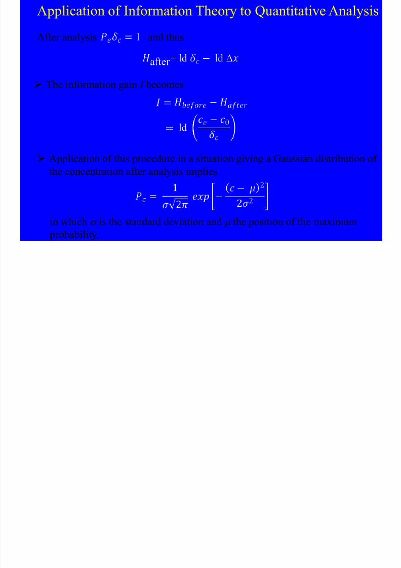
8/10/2019 Kimia Analitik Lanjut
http://slidepdf.com/reader/full/kimia-analitik-lanjut 188/270
for skewness. It signals a symmetry of the distribution. Although a pas
test for skewness does not necessarily prove that the distribution is
normal, a failed test obviously indicates that normal statistics should b
applied with care.A parameter for skewness is the so-called third moment, denoted by m3:
Data Processing
Tests for Normality
An index of skewness that is independent of the unit of measurements
the third moment divided by the cube of the standard deviation. This
parameter is denoted by √b1:

8/10/2019 Kimia Analitik Lanjut
http://slidepdf.com/reader/full/kimia-analitik-lanjut 189/270
The value of √ b 1 should be zero, but since s normally is not known an
is estimated by s, and because the third moment is also an estimation,some deviation from zero is allowed. Table below gives the probability
various deviations from zero for a normal distribution.

8/10/2019 Kimia Analitik Lanjut
http://slidepdf.com/reader/full/kimia-analitik-lanjut 190/270
Data Processing
Tests for Normality → Graphic Kolmogorov Test 1. Arrange the data in ascending order.
2. Draw the cumulative frequency line for a normal distribution (G in the
Figure below)

8/10/2019 Kimia Analitik Lanjut
http://slidepdf.com/reader/full/kimia-analitik-lanjut 191/270
3. Draw two lines parallel to the line of step2, each at a distance D ; D ca
be obtained from Table below
Cumulative frequency for Kolmogorov test
Graphic Kolmogorov Test

8/10/2019 Kimia Analitik Lanjut
http://slidepdf.com/reader/full/kimia-analitik-lanjut 192/270
4. Draw the cumulative frequency line of the ordered data (S in the Figure
above)
5. If S is found somewhere out side the lines of step3, the distribution cy an
considered not normal with a probability given by the chosen value of Taabove.
Numerical Kolmogorov Test
1. Arrange the data in ascending order.
2. Compute Di = S ( xi) – i/n, with i = sequential data points or frequencies, n
total number of data points, and S ( xi) = corresponding normal cumulative
distribution values.
3. Select the maximum value ( Dm) of Di.

8/10/2019 Kimia Analitik Lanjut
http://slidepdf.com/reader/full/kimia-analitik-lanjut 193/270
4. If Dm is larger than value given by the Table 4.3, the distribution can be
considered as not normal, with a probability given by the selected a-valu
of Table 3.
An example of both methods is given in the Figure and Table below

8/10/2019 Kimia Analitik Lanjut
http://slidepdf.com/reader/full/kimia-analitik-lanjut 194/270
Transformation of Data
Data Processing
Occasionally one encounters a distribution that, by one of the tests
mentioned above, departs too far from normality. It would not be safe the
to apply the statistical tests, and it would be a great advantage if, by a sim
transformation of the variable ,an approximately normal distribution coul
be obtained.

8/10/2019 Kimia Analitik Lanjut
http://slidepdf.com/reader/full/kimia-analitik-lanjut 195/270
A universally applicable transformation for nonnormal data sets to be
created as sets that are as near to normality as possible can be written for
theoretical reason as follows:
Where xi = the measured quantity; = the transformed datum; l = thetransformation parameter; c = constant.
Transformation of Data
Data Processing
For practical applications the equation can be reduced to
The transformation is applied for a range of values of l and each time a tfor normality is performed. The best value of l is chosen.
Th t f ti l ti d b i li d i th ft d

8/10/2019 Kimia Analitik Lanjut
http://slidepdf.com/reader/full/kimia-analitik-lanjut 196/270
The transformation rules mentioned above are implied in the often used
“intuitive” transformations:
l Transformation
2 Square
1 Unaltered
0.5 Square root
0.333 Cube root
0 log-1 Reciprocal
Information Theory
Analytical chemistry provides optimal strategies for collecting andappreciating irrelevant information on situations and processes in materia
The input into the analytical procedure contains some actual informat
and some latent information (uncertainty).
During the analytical process the actual information increases at theexpense of the latent information.

8/10/2019 Kimia Analitik Lanjut
http://slidepdf.com/reader/full/kimia-analitik-lanjut 197/270
For example, a sample is analyzed for iron content.
The actual information here is that iron is expected to be present an
the amount is to be determined. The latent information is the unknown quantity of iron.
By an analytical procedure the iron content is measured and found
be 10.82± 0.01% weight.
Thus the uncertainty is decreased from a range of 0 - 100% to that
10.81-10.83% at the expense of the latent information.
Information Theory
The output of analytical chemistry is information that is disclosed by
measurements, the definition of this quantity needs a closer examination.
Information equals diminishing uncertainty, as in an example of the iron
content before analysis equals 0 - 100% and afterward 10.81-10-83%.
General definition of information I equals uncertainty H before - H after analy
Another name for uncertainty H is entropy. The magnitude of H is given b

8/10/2019 Kimia Analitik Lanjut
http://slidepdf.com/reader/full/kimia-analitik-lanjut 198/270
the number of possibilities (n) before and after the experiment. The most
simple experiment is a decision between two alternatives, yes or no.
The yield of information of such an experiment is selected as a unit of
information, the bit (binary unit). This selection implies
and k = l/logz 2. Thus
ld represents the logarithm with base 2. Other units found in literature are
"nit," based on logarithm with base e, and "dit," based on informationobtained by selecting 1 out of l0 independent possibilities.
Information Theory
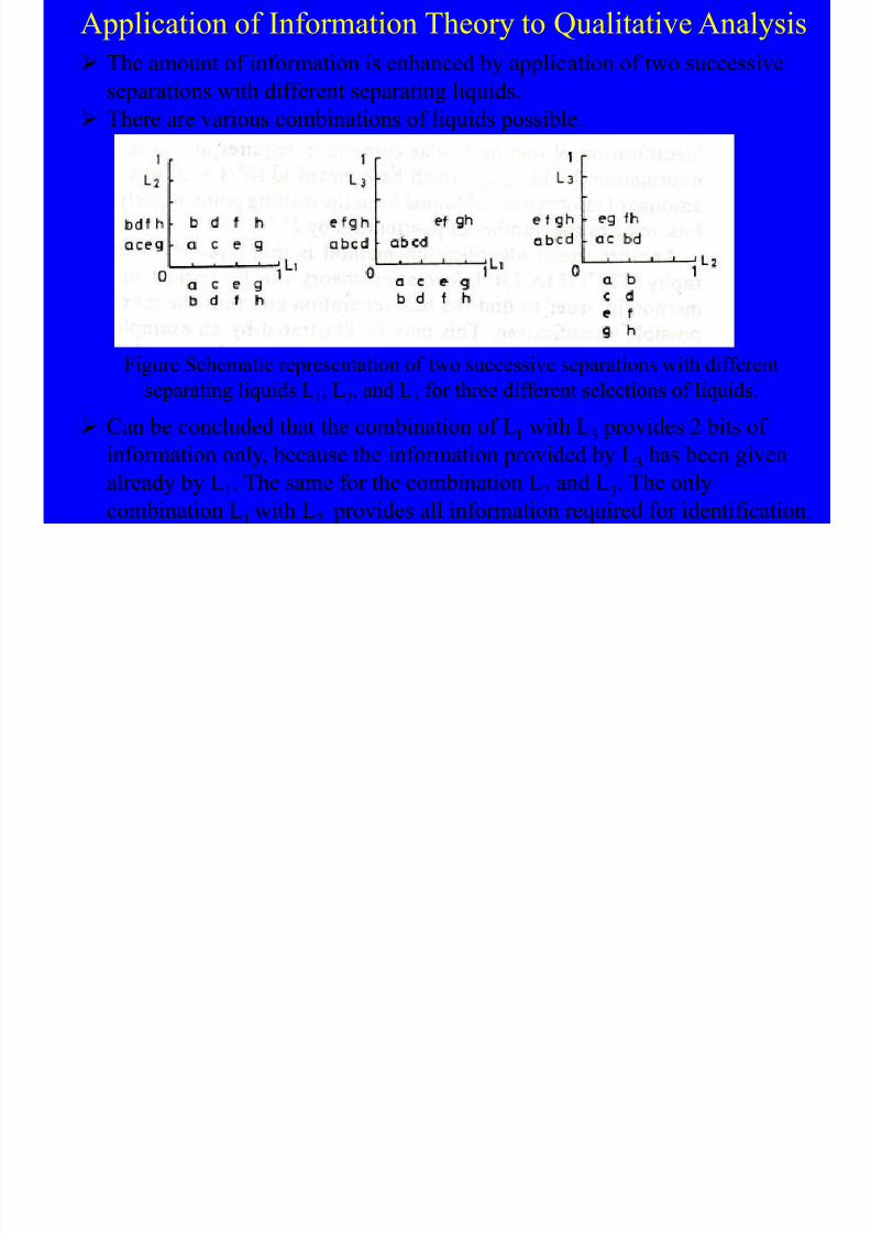
8/10/2019 Kimia Analitik Lanjut
http://slidepdf.com/reader/full/kimia-analitik-lanjut 199/270
If a selection must be made of 1 out of n possibilities with unequal
possibilities, the equation of Shannon should be applied
Information Theory
A possibility to be mentioned is a probability distribution represented by Gaussian function.
Such a distribution may be approximated by means of a histogram with
given width of the classes Dx. The smaller is Dx, the more classes are
needed and the better the approximation.
The probability of occurrence of a given class equals

8/10/2019 Kimia Analitik Lanjut
http://slidepdf.com/reader/full/kimia-analitik-lanjut 200/270
The entropy of a real continuous distribution may be approximated by entropy of the histogram
Application of Information Theory to Quantitative Analy
The constant Pc of a certain compound in a mixture before and after analyis depicted as follows:
Figure. Probability of occurre
of a concentration P as a funct
of the numerical value of thatconcentration C before (P b) an
ft (P ) l i

8/10/2019 Kimia Analitik Lanjut
http://slidepdf.com/reader/full/kimia-analitik-lanjut 201/270
Before the analysis each concentration co and ce has an equal probability occurrence; after analysis the concentration is known with a deviation of
Application of the Shannon equation to the situation before analysis yield
after (Pa) analysis
Application of Information Theory to Quantitative Analy
and after analysis

8/10/2019 Kimia Analitik Lanjut
http://slidepdf.com/reader/full/kimia-analitik-lanjut 202/270
Before analysis
or
Application of Information Theory to Quantitative Analy
After analysis and thus
The information gain I becomes

8/10/2019 Kimia Analitik Lanjut
http://slidepdf.com/reader/full/kimia-analitik-lanjut 203/270
Application of this procedure in a situation giving a Gaussian distributionthe concentration after analysis implies
in which s is the standard deviation and m the position of the maximum probability.
This distribution results in the following H a value:
Application of Information Theory to Quantitative Analy
and thus
In situations where s is unknown, its value may be estimated frommeasurements and the mean result of the measurement :

8/10/2019 Kimia Analitik Lanjut
http://slidepdf.com/reader/full/kimia-analitik-lanjut 204/270
A somewhat more generale expression is given by
Here t p,v represents the probability distribution of the analytical results p and
parameter v, representing the number of degrees of freedom.
Application of Information Theory to Quantitative Analy
The gain of information depends on s and n. The increase in the number omeasurements is not proportional to the increase of information: the incre
of information is less than the information expected from the number of
measurements.
The diminishing effect of the estimated number of measurement on
information gain is called redundancy R :

8/10/2019 Kimia Analitik Lanjut
http://slidepdf.com/reader/full/kimia-analitik-lanjut 205/270
This equation implies that the maximum amount of information to be
gained from n measurements equals n times the information of one sinmeasurement. The interaction between successive measurements thus
supposed to be absent. In the case that correlation exists between
measurements
corr = correlation matrix
Application of Information Theory to Quantitative Analy
The redundancy provides a method for estimation of the mutual interactioof successive measurements. A high value of the redundancy implies that
effects of interruptions otherwise leading to erroneous results are partially
canceled by the correct results in a series of measurements.
In quantitative analysis a calibration graph frequently is used. The questiothen arises: how is the information theory applied here? To begin with, th
standardized function u = ac + b is constructed from m samples with

8/10/2019 Kimia Analitik Lanjut
http://slidepdf.com/reader/full/kimia-analitik-lanjut 206/270
p
concentrations ci and measurements ui
The analysis of a sample yields a measurement ua and thus a concentratio
co. A set of n parallel measurements result in and .
With a linear dependence of c on u the error in ca, Dca, equals
Application of Information Theory to Quantitative Analy

8/10/2019 Kimia Analitik Lanjut
http://slidepdf.com/reader/full/kimia-analitik-lanjut 207/270

8/10/2019 Kimia Analitik Lanjut
http://slidepdf.com/reader/full/kimia-analitik-lanjut 208/270

8/10/2019 Kimia Analitik Lanjut
http://slidepdf.com/reader/full/kimia-analitik-lanjut 209/270

8/10/2019 Kimia Analitik Lanjut
http://slidepdf.com/reader/full/kimia-analitik-lanjut 210/270

8/10/2019 Kimia Analitik Lanjut
http://slidepdf.com/reader/full/kimia-analitik-lanjut 211/270
Application of Information Theory to Qualitative Analys
An accuracy of the melting point measurement corresponds with the widtof the classes in the histogram, the information yield of a melting point
measurement equals
A more accurate measurement of the melting point results in a relativelysmaller reliability interval in comparison with the width of a class and
correspondingly provides more information.

8/10/2019 Kimia Analitik Lanjut
http://slidepdf.com/reader/full/kimia-analitik-lanjut 212/270
To account for this effect, it is assumed an accuracy for the melting points
equal to k times that of the histogram intervals. The melting pointmeasurement may be considered as a combination of two experiments
1. A class selection procedure with an information yield of
2. Within a class selection of 1 possibility out of a set of k , with an
information yield of I 2 = ld k , or in terms of class broadness D x and
reliability interval D y, I 2 = ld D x/D y
Application of Information Theory to Qualitative Analys
The total amount of information thus becomes
This calculation implies equal probability for all k possibilities within a
given class. In many situations this is not true. In order to deal withsituations where the probability of the situations are not equal, a probabi
distribution function within a class may be defined.

8/10/2019 Kimia Analitik Lanjut
http://slidepdf.com/reader/full/kimia-analitik-lanjut 213/270
The equations involved in such situations are
for information obtained of intraclass distribution and
Application of Information Theory to Qualitative Analys
For information of intraclass distribution in class i, q j, equals the probabof occurrence of the measured melting point in graph j of class i.
The average intraclass in formation , for the entire histogram equals
which makes the total information

8/10/2019 Kimia Analitik Lanjut
http://slidepdf.com/reader/full/kimia-analitik-lanjut 214/270
which makes the total information
Application of Information Theory to Qualitative Analys
The equation above refers to the distribution of melting point over a newhistogram with class width m. Based on the histogram and an accuracy ooC in the measurement of the melting points, an amount of information m
be obtained
Based on an estimated number of 106 compounds, the identification of on

8/10/2019 Kimia Analitik Lanjut
http://slidepdf.com/reader/full/kimia-analitik-lanjut 215/270
particular compound requires an amount of information I = ld n0/n1, whic
here means ld 106/1 = 20 bits.
The amount of information obtained from the melting point, namely, 8 bits, reduces the number of possibilities by 28,5 ≈ 360.
Another useful identification method is thin-layer chromatography
(TLC). Information theory can be applied to this method in order to fin
the best separation and thus the maximal possible identification.
Application of Information Theory to Qualitative Analys
To identify one particular compound out of a set of 8, an amount ofinformation of ld 8 = 3 bits is required.
A theoretical solution for this identification problem is provided by two
separating schemes, one giving 2 bits of information and the other 1 bit.
In practice this solution is not always possible because part of the
information provided by the first solvent may be identical with that
given by the second solvent, which results in a total gain of informatio
of less than 3 bits

8/10/2019 Kimia Analitik Lanjut
http://slidepdf.com/reader/full/kimia-analitik-lanjut 216/270
of less than 3 bits.
most information is obtained from a combination of two separating
solvents with the highest possible independent information yield.
It is concluded from the RF values that the individual liquids do not provi
enough information for the identification of the compounds a-h (see Tabl
below).
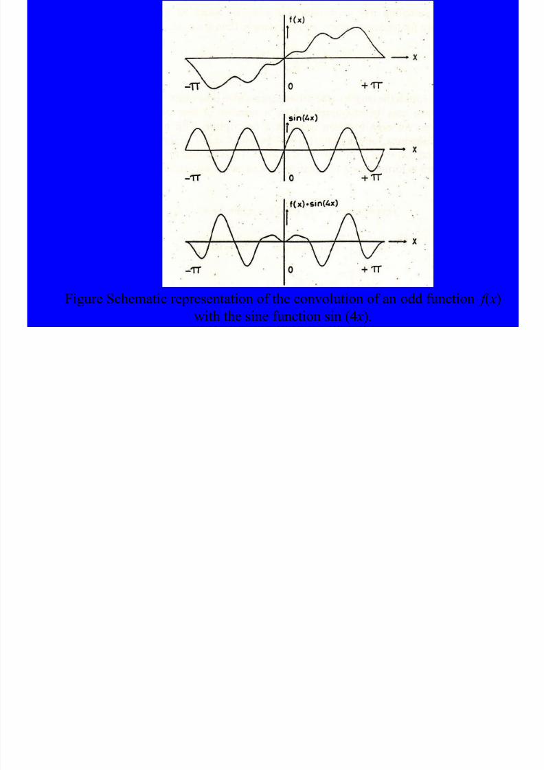
8/10/2019 Kimia Analitik Lanjut
http://slidepdf.com/reader/full/kimia-analitik-lanjut 217/270
Application of Information Theory to Qualitative Analys
The amount of information is enhanced by application of two successiveseparations with different separating liquids.
There are various combinations of liquids possible.

8/10/2019 Kimia Analitik Lanjut
http://slidepdf.com/reader/full/kimia-analitik-lanjut 218/270
Can be concluded that the combination of L1 with L3 provides 2 bits of
information only, because the information provided by L3 has been given
already by L1. The same for the combination L2 and L3. The onlycombination L1 with L2 provides all information required for identificatio
Figure Schematic representation of two successive separations with different
separating liquids L1, L2, and L3 for three different selections of liquids.
Filtering
In order to apply measured quantities, in most situations the following
treatment is required:
Removal of nonessential-irrelevant-data (noise)
Reconstruction of essential data
Interpretation of data

8/10/2019 Kimia Analitik Lanjut
http://slidepdf.com/reader/full/kimia-analitik-lanjut 219/270
Removal of Irrelevant Data (Noise) Noise is the undesired part of a signal.
It is impossible, in practice, to separate noise completely from the rest of
the signal because each noise filter generates noise itself.
A practical yardstick for the applicability of a signal is provided by the
signal-to-noise (SA) ratio.
to measure this ratio one starts by measuring the available power of th
signal wave and of the noise wave

8/10/2019 Kimia Analitik Lanjut
http://slidepdf.com/reader/full/kimia-analitik-lanjut 220/270
s g w ve d o e o se w ve
In direct current signals the power is proportional to the voltage E; in
alternating current signals it is proportional to the root mean square va
Arms of the waveshape:
with being the average value of the waveshape, and Ai the deviation
the i th measurement from the average
Removal of Irrelevant Data (Noise)
With direct current signals sampled at discrete time intervals the main paof the noise is governed by a variation with time of the signal. The noise
given by the standard deviation of the signal and thus the signal-to-noise
ratio becomes
This equation gives a simple method to calculate S/N from a recorder
signal

8/10/2019 Kimia Analitik Lanjut
http://slidepdf.com/reader/full/kimia-analitik-lanjut 221/270
signal.
For example, 99% of all observations is found between m - 2.5s and
m + 2.5s (m equals the main value, and s denotes the estimated standarddeviation). Here S/N equals 0.2, the peak-to-peak variance of the signal.
The observation period should be long enough to enable a reliable estima
of S . It is assumed that the signal is distributed around the average value
according to a Gaussian distribution.
Removal of Irrelevant Data (Noise) Other techniques, for example autocorrelation, should be applied for
calculating S/N, where alternating current signal are measured.
Various types of noise that can be recognized by their frequency spectrum
White noise −has a frequency spectrum with a flat shape. It caused by
random processes such as Brownian motion, external influence, andthermal motion of electrons (Johnson noise).
1/f noise −where the power is proportional to 1/ f . Such a situation is
met with for example a drifting signal

8/10/2019 Kimia Analitik Lanjut
http://slidepdf.com/reader/full/kimia-analitik-lanjut 222/270
met with, for example, a drifting signal.
Red noise −contains more low-frequency noise than the averae value.
Blue noise −contains more high-frequencyn oiset han the averae valu Interference noise −nearly always results from external source with
relatively low chance of occurrence, i.e., switching on or off on powe
undesired components in a spectrum, and so on.
Removal of Irrelevant Data (Noise) A special form of interference noise is impulse noise caused by source
such as the starting up of a powerful engine. All frequencies are met in
this type of noise, making it difficult to eliminate.
Another type of interference noise is deformation noise. Here some
specific frequencies are added to or removed from the signal. Some
possible causes of deformation noise are nonlinearity of the instrumen
transmission losses and reflections.

8/10/2019 Kimia Analitik Lanjut
http://slidepdf.com/reader/full/kimia-analitik-lanjut 223/270
Frequency spectrum of "white" noise and of "l/ f " noise

8/10/2019 Kimia Analitik Lanjut
http://slidepdf.com/reader/full/kimia-analitik-lanjut 224/270
Digital Filtering
The equation describes how to calculate a new S , value from an older S t by adding a new measured quantity xt and eliminating the oldest xt-N .
Exponential smoothing requires considerably less storage capacity; becau
nonavailable data are substituted by the mean value: ( xt – xt-N )/ N in previ
equation is replaced by ( xt – S t-1)/ N ′. S t equals the running exponential
mean at time t , and N ' the mean length of the averaging period.Substitution of a : N '-1 yields

8/10/2019 Kimia Analitik Lanjut
http://slidepdf.com/reader/full/kimia-analitik-lanjut 225/270
the new S t value is obtained from the old by correcting with the scaled
difference between the old value and the most recently measured value.
The scaling factor a is inversely proportional to the length of the runn
interval.
Digital Filtering
Digital signal averaging is a commonly used technique that requires a
many channels as signals to be averaged. Interference noise is notaveraged out by signal averaging.
Th l t d i l b l l di ti i h bl b i i
The advantage of this method over the previous one is that only thmean value S t-1 has to be stored in memory; all measured values ar
accounted for, in contrast to the running average method.

8/10/2019 Kimia Analitik Lanjut
http://slidepdf.com/reader/full/kimia-analitik-lanjut 226/270
The correlated signals become clearly distinguishable because noise i
eliminated. The correlation time may be used to describe the signal.
Kalman Filtering
Kalman showed that there exists an optimal estimation method that is eve
better than the exponential smoothing method.
A measured quantity yt , obtained at time t , is just a momentary
description of a situation that takes no account of the history of a time
series of measurements.
It is possible to make a better estimate of reconstructed values out of a
time series at time t and to predict the value of new measurements taki
into account the history of that time series. Here the prediction of a

8/10/2019 Kimia Analitik Lanjut
http://slidepdf.com/reader/full/kimia-analitik-lanjut 227/270
measured value is based on the most recent measurement, and the
expected value is corrected with the values measured in the more dista
past. The weight of the predicting capacity of the measured values fro
the past decreases with increasing distance from the present time. The
application of this technique is called exponential smoothing.
The predicted value for time t , called i, is combined with a measured
value yt , in order to construct a better estimate called* , (eacho f the d
Kalman Filtering
The predicted value for time t , called , is combined with a measured
value yt , in order to construct a better estimate called , (each of the d
xt and yt contains errors, which makes an exact prediction impossible)
Analytical chemistry can be described by a set of very simple equations:
o Here X k, often called the state of the system, can be a concentration

8/10/2019 Kimia Analitik Lanjut
http://slidepdf.com/reader/full/kimia-analitik-lanjut 228/270
k , y ,
o The equation describes the concentration at time (or sequence) k to
a function of the past; F k is a transition function.o In the case of a stable sample where the concentration will not chan
in time, F k will be 1.
o In the case of a process, F k can for instance be F k = exp(−ak )
o The value of X k will be between certain values we do not know, this
denoted bv W k-1, the systetn error.
Kalman Filtering
o The equation gives the relation between state (e.g., the concentration)
and a measured value X k .
o H k can be the calibration factor, and V k denotes the measurement erro
Now X k can be predicted:

8/10/2019 Kimia Analitik Lanjut
http://slidepdf.com/reader/full/kimia-analitik-lanjut 229/270
Kalman Filtering
The weight factor K k , determining the relative weights of the present history, can be estimated from
where is the variance in the systern, and Rk is the variance of the
measurement ( Rk = V 2). So a high value of Rk (a high measurementnoise) sets K k to be low and the values from the past get a higher weig
through previous equation.

8/10/2019 Kimia Analitik Lanjut
http://slidepdf.com/reader/full/kimia-analitik-lanjut 230/270
A larger uncertainty in the system ( P k high) gives more weight to the
measurement. Then can be predicted from
and P k can be estimated from
Kalman Filtering
As this set of equations is recursive a starting value for X k and P k isrequired. These can be guessed from past experience or, when such
experience is lacking, X k can be set to 0, P k to a high value.
As the advantage of the Kalman filter is the exploitation of the
knowledge obtained in the past and updating this knowledgecontinuously, the method can be used to enhance the quality of
analytical measurements

8/10/2019 Kimia Analitik Lanjut
http://slidepdf.com/reader/full/kimia-analitik-lanjut 231/270

8/10/2019 Kimia Analitik Lanjut
http://slidepdf.com/reader/full/kimia-analitik-lanjut 232/270
Fourier Convolution
A smoothing filter acts to block high frequencies and allow only low-
frequency signals to pass.
Some examples of smoothing filters are a triangular function ( x = 0, y
1 and x ≥ a, y = 0); the half of a Gaussian function ( x = 0, y = ymax and
x = a, y → 0); and a decreasing exponential function.
The selection of an appropriate smoothing function is a matter of trial
and error. Sometimes the characteristics of the instrument under
consideration are measured under high signal-to-noise conditions.

8/10/2019 Kimia Analitik Lanjut
http://slidepdf.com/reader/full/kimia-analitik-lanjut 233/270
These characteristics are used afterward in a convolution of signalsmeasured under conditions with high noise levels. Here the spectrum
including noise is convoluted by means of a Fourier transform with a
virtually noise-free signal.
In the frequency domain convolution means multiplication; the place o
time domain asks for a much more elaborate process for convolution.
Here the convolution integral means
T ( y) represents a virtually noise-free convoluted signal: t ( x), the observed
signal: and B( y - x), the smoothing function.
A disadvantage of convolution should be mentioned here: together with t
noise part of the signal, a distortion of the signa loccurs which manifests
Fourier Convolution
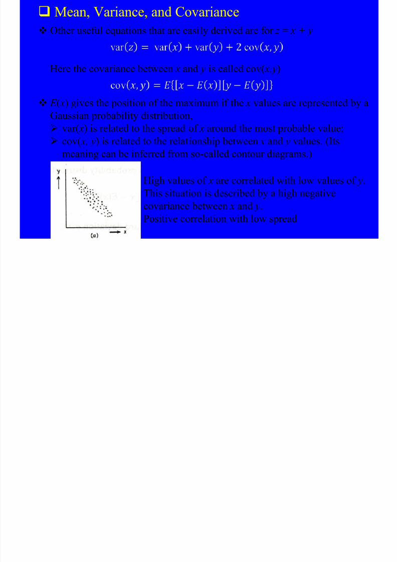
8/10/2019 Kimia Analitik Lanjut
http://slidepdf.com/reader/full/kimia-analitik-lanjut 234/270
itself as a broadening of the peaks (and a lowering of the maximal signal
values because of normalization).
Fourier Convolution
A time series is written as a summation of a number of sine and cosine
terms. This procedure is allowed for each type of function f ( x):
f ( x) = a1 sin x + a2 sin 2 x + a3 sin 3 x + ···· + bo + b1 cos x + ···· + bn cos
In order to calculate the coefficients am, f ( x) is multiplied by sin mx dx (m
1, 2, ...) and integrated between - p and p. This process is visualized asshown in the Figure below.
It is seen that even functions "f(x) = +f(− x)" make all a coefficients zero

8/10/2019 Kimia Analitik Lanjut
http://slidepdf.com/reader/full/kimia-analitik-lanjut 235/270
It is seen that even functions f ( x) + f ( x) make all a coefficients zero
and odd functions “ f (x) = − f (− x)" make all a coefficients zero.
In situations where the periodicity of sin mx corresponds with a periodici
of f ( x), the product function does not change sign because a change in sig
of sin mx occurs at the same x value where a change in sign of f ( x) occur.

8/10/2019 Kimia Analitik Lanjut
http://slidepdf.com/reader/full/kimia-analitik-lanjut 236/270
Figure Schematic representation of the convolution of an odd function f ( x
with the sine function sin (4 x).
Deconvolution
Deconvolution offers a method of eliminating distortions of signals that a
caused by the instrument. Here one aims for the recovery of the original
signal, for example, by application of Fourier transform analysis.
As an example the distortion of an optical signal caused by the slit of t
instrument is considered.
The shape of the distorted signal is known to be a broadened line, andorder to recover the original line shape a transformation is required tha
performs the opposite of a convolution calculation:

8/10/2019 Kimia Analitik Lanjut
http://slidepdf.com/reader/full/kimia-analitik-lanjut 237/270
T ( y) represents the broadened signal, distorted by the Fourier transform
(FT) of the slit width function B( y - x); t ( x) equals the undistorted signal
wants to recover. The aim of the deconvolution process is the recovery of
f ( x).
In the frequency domain deconvolution means division of the FT of the
observed signal by the FT of the distorting function and backtransformatof the resulting FT of the undistorted signal
Deconvolution
The deconvolution process is depicted schematically as follows:
Removal of signal broadening by
deconvolution of the Fourier transform

8/10/2019 Kimia Analitik Lanjut
http://slidepdf.com/reader/full/kimia-analitik-lanjut 238/270
deconvolution of the Fourier transform
(FT) of the distorted signal by the FT of t
distorting signal followed by the reversetransformation
Deconvolution
The deconvolution results in a smaller line width and thus allows a better
peak separation. However, the deconvoluted signal shows some little extrsignals that are not found in the original spectrum. These signals are
artificial and hamper the detection of low-intensity signals that actually
might be present in the original signal.
In situations where the slit function (or other artificial disturbances due tothe instrument) is unknown it should be measured separately.
A general procedure accepted in spectrometry is to proceed as follows
A spectrum of a component of a mixture is recorded with a narrow slit

8/10/2019 Kimia Analitik Lanjut
http://slidepdf.com/reader/full/kimia-analitik-lanjut 239/270
p p
width A and another recording is made with identical parameter setting
except for a large slit width B. It is to be noted that recording A gives a better peak separation than recording B. Now the Fourier transformed
spectrum B is divided by the FT of spectrum A in order to produce the
of the slit function C. The back-transformation of C„ yields the slitfunction in the l domain and may be used for transformation purposes
future spectra.
Data Reconstruction and Curve Fitting
The production of measuremnts by one-dimensional methods of analysissuch as melting points, boiling points, indexes of refraction, and so on
mostly do not present problems.
A multiplication or division usually suffices for reconstruction of relev
information.
The situation becomes more complicated for two-dimensional methodanalysis such as are encountered in spectral analysis.
The analysis means measurement of peak positions and of the heights
peak surface.
Diffi l i b d b h f ll i

8/10/2019 Kimia Analitik Lanjut
http://slidepdf.com/reader/full/kimia-analitik-lanjut 240/270
Difficulties may be caused by the following:
• Noise and drift on the original spectra. Noise may be eliminated by smoothing (the l and the intensity sc
respectively) may be corrected by the application of calibration da
stored in advance.
Baseline detection eliminates drift and the disturbances caused by
functions can be corrected by deconvolution.
Data Reconstruction and Curve Fitting
• Overlapping peaks. Positions of peaks can be found by differentiating the original
spectrum as a function of time or wavelength.
A stronger overlap asks for more consecutive differentiations in o
to establish peak position.
In practice the number of differentiations is limited because eachdifferentiation enhances the noise.
The peak surface is found by integration over time or wavelength
In order to obtain accurate peak surfaces the baseline should be w
d fi d

8/10/2019 Kimia Analitik Lanjut
http://slidepdf.com/reader/full/kimia-analitik-lanjut 241/270
defined.
• A baseline mot sufficiently well known.
The baseline is parts of a spectrum where no peaks are found.
A baseline correction is only possible when such parts occur.

8/10/2019 Kimia Analitik Lanjut
http://slidepdf.com/reader/full/kimia-analitik-lanjut 242/270
In spectroscopy symmetrical peaks are mostly described• by the Lorentz function
• by the Gauss function
• by linear combinations of these functions. AL and A0 are found from
intensity and/or normalization conditions such as
Data Reconstruction and Curve Fitting

8/10/2019 Kimia Analitik Lanjut
http://slidepdf.com/reader/full/kimia-analitik-lanjut 243/270
and B represents a relationship with width at half height W: BL = 2/W;
. Nonsymmetric peaks are approximated by means o
empirically adapted standard digital functions. The estimated line shape
can be approximated as accurately as desired by enhancement of the
number of points in the digital function.
Curve Fitting Curve fitting aims for a mathematical description of a series of measured
data by a model with adaptable parameters. In general, the following procedure is applied:
• A mathematical model is chosen on the basis of empirical knowled
on the system under investigation (e.g., Lorentzian line shape or
Gaussian line shape).
• The adaptable parameters in o be determined such as the model sucas line width, peak position, and peak height are calculated in a
manner that makes the sum of the squares of the deviations betwee
calculated and measured data points as small as possible.

8/10/2019 Kimia Analitik Lanjut
http://slidepdf.com/reader/full/kimia-analitik-lanjut 244/270
p p
• The number of parameters to be found equals the number of peaks
multiplied by the number of parameters per peak.
Suppose the analytical function that is going to represent the measured d
equals
a 1, .., a n are parameters to be determined, i.e., line width and peak positi
y = f (a 1, a 2, a 3, ......., a n, x)
Curve Fitting It is assumed that the number of measured data m is greater than the num
of independent parameters n. The residual sum of squares R that represen
the differences between the calculated values and the measured data Y , is
defined by
and has to be minimized with respect to each a i . The condition

8/10/2019 Kimia Analitik Lanjut
http://slidepdf.com/reader/full/kimia-analitik-lanjut 245/270
yield n equation of the form

8/10/2019 Kimia Analitik Lanjut
http://slidepdf.com/reader/full/kimia-analitik-lanjut 246/270
Curve Fitting
Properties of curve fitting by least-squares procedures may be summarize
as follows:
• All data must be stored in a data set before the calculations can be
started.
• The baseline adaptation should be taken into account.
• Partial derivatives with respect to all adaptable parameters should becalculated at each position of the spectrum. Sometimes this calculation
must be repeated at each iteration cycle.
• Matrix manipulations are necessary.
• The starting parameters should be estimated The possible dependence

8/10/2019 Kimia Analitik Lanjut
http://slidepdf.com/reader/full/kimia-analitik-lanjut 247/270
• The starting parameters should be estimated. The possible dependence
the solution on the starting parameters must always be tested.• Convergence may be accelerated by properly diminishing the paramst
variations.
• The whole procedure may be a failure if an inappropriate mathematica
model is selected.

8/10/2019 Kimia Analitik Lanjut
http://slidepdf.com/reader/full/kimia-analitik-lanjut 248/270

8/10/2019 Kimia Analitik Lanjut
http://slidepdf.com/reader/full/kimia-analitik-lanjut 249/270

8/10/2019 Kimia Analitik Lanjut
http://slidepdf.com/reader/full/kimia-analitik-lanjut 250/270

8/10/2019 Kimia Analitik Lanjut
http://slidepdf.com/reader/full/kimia-analitik-lanjut 251/270
Mean, Variance, and Covariance
For g ( x) = ax, a representing a constant, this results in
This equation also holds for the continuous probability distribution funct
Apart from the expectation value or mean value of x one may also be
interested in the spread of x values over the series of measurement in ord
to gain insight into the reproducibility of the measurements. The statistic
expression applicable here is the variance of x

8/10/2019 Kimia Analitik Lanjut
http://slidepdf.com/reader/full/kimia-analitik-lanjut 252/270
expression applicable here is the variance of x,
Mean, Variance, and Covariance
in the situation with a continuous probability distribution of x,
Another expression used is the standard deviation s ( x):
again selecting the situation E (ax) one may derive

8/10/2019 Kimia Analitik Lanjut
http://slidepdf.com/reader/full/kimia-analitik-lanjut 253/270
and
where is the absolute value of a
Mean, Variance, and Covariance
Other useful equations that are easily derived are for z = x + y
Here the covariance between x and y is called cov( x,y)
E ( x) gives the position of the maximum if the x values are represented byGaussian probability distribution,
var( x) is related to the spread of x around the most probable value;
cov( x, y) is related to the relationship between x and y values. (Its
i b i f d f ll d t di )

8/10/2019 Kimia Analitik Lanjut
http://slidepdf.com/reader/full/kimia-analitik-lanjut 254/270
meaning can be inferred from so-called contour diagrams.)
High values of x are correlated with low values of y
This situation is described by a high negative
covariance between x and y.
Positive correlation with low spread

8/10/2019 Kimia Analitik Lanjut
http://slidepdf.com/reader/full/kimia-analitik-lanjut 255/270
Mean, Variance, and Covariance
The magnitude of the covariance can be standardized. The standardized
covariance is called the correlation coefficient r ( x,y):
in which s ( x) = [var( x)]1/2.
A special situation is met when y = ax (a ≥ 0).

8/10/2019 Kimia Analitik Lanjut
http://slidepdf.com/reader/full/kimia-analitik-lanjut 256/270
Thus
Mean, Variance, and Covariance
In situations where the value found for x fixes completely
the value to be expected for y, r ( x,y) =± 1.
Where no relationship exists cov( x,y) = 0 and thus r ( x,y) = 0.
In the situations considered so far x as well as y pertain to stationary state
This changes when time-dependent processes are considered. Here the
measured values x vary with time.
The collected values x over a period of time are called a time series.

8/10/2019 Kimia Analitik Lanjut
http://slidepdf.com/reader/full/kimia-analitik-lanjut 257/270

8/10/2019 Kimia Analitik Lanjut
http://slidepdf.com/reader/full/kimia-analitik-lanjut 258/270
Time Series The notation of a time series:
Observations are made at times T0, T1, T2,.. .,Tn, giving observed valuZ(T0), Z(T1),..., Z(Tn).
In situations where the time interval between two successive
measurements is a constant h the notation may conveniently be change
into:
For a starting time To = 0 and h equal to the unit of time, Zt , becomes the
measurement at time t .
− measuring time To, To+ h, To + 2h,...,To + nh
− measurements Zo, Z1, Z2,..., Zn

8/10/2019 Kimia Analitik Lanjut
http://slidepdf.com/reader/full/kimia-analitik-lanjut 259/270
In practice two types of time series may be distinguished: Deterministic time series − in which the future is conrpletely determin
such as Zt = cos (2p ft )
Statistical time series − in which the values expected may be forecast
terms of a probability distribution function
Time Series
A statistical phenomenon that develops in time according to probability
laws is called a stochastic process.

8/10/2019 Kimia Analitik Lanjut
http://slidepdf.com/reader/full/kimia-analitik-lanjut 260/270
Figure . Example of a stochastic process Z(t) as a function of time with its
probability distribution function P z (t )
Time Series
A stationary process is a special type of stochastic process:
it is a process in statistical equilibrium, which means that the propertieof the process do not depend on the starting time of the observation
period.
Such a process can be subdivided into parts so that all may start at tim
To,.
The subdivision is allowed, provided that a minimal realization lengthobtained or surpassed. Such signals with equal statistical properties ar
called ergodic.
Because the process is statistically determined, each time t provides a
b bilit di t ib ti f Z Thi i li th t ti i f M

8/10/2019 Kimia Analitik Lanjut
http://slidepdf.com/reader/full/kimia-analitik-lanjut 261/270
probability distribution for Z . This implies that a time series of M
observations should be represented by an M-dimensional vector ( Z 1,
Z 2,..., Z m) with a probability distribution P ( Z 1, Z 2,..., Z m).
Given a stationary process, the condition holds that m measurements Z
Z t 2, ..., Z tm measured at time t 1, t 2,...,t m are the same as the measuremen
Z t 1+t, Z t 2+t, ..., Z tm+t measured at time t 1+t, t 2+,...,t m+t
Time Series
Two important properties of stationary processes are the following:
• The mean value m is a constant given by
• The variance of Z is a constant
In the special situation m = 1 the probability distribution P ( Z t ) is the sam
for all t values and can be denoted as P ( z ).

8/10/2019 Kimia Analitik Lanjut
http://slidepdf.com/reader/full/kimia-analitik-lanjut 262/270
P ( z ) can be found from a histogram of measurements on time series Z 1, Z Z 3,..., Z n because P ( z ) is a constant for all values of t . The average value m
from a stationary process is found from the average value of the time
series of n → ∞
the variance:
Time Series
For a stationary process the probability of occurrence of a pair of
measurement P ( Z t 1, Z t 2) is a constant for all times t 1 and t 2 provided that ttime interval between t 1 and t 2 is a constant. This is illustrated in Figure
below, where it is apparent that the correlation between Z t +1 and Z t is high
than the between Z t +5 and Z t . In general the correlation decreases upon an
increase of t.

8/10/2019 Kimia Analitik Lanjut
http://slidepdf.com/reader/full/kimia-analitik-lanjut 263/270
Decrease in correlation with increasing time span of a time series Z(t )
Autocorrelation
The covariance between X t , and Z t+t of a time series can be calculated a
is called the autocovariance g t (auto because one stays within the timeseries):
The collection of g t values for various values of p normalized to thevariance is called the autocorrelation function r t:

8/10/2019 Kimia Analitik Lanjut
http://slidepdf.com/reader/full/kimia-analitik-lanjut 264/270
Because for a stationary process,
implying

8/10/2019 Kimia Analitik Lanjut
http://slidepdf.com/reader/full/kimia-analitik-lanjut 265/270

8/10/2019 Kimia Analitik Lanjut
http://slidepdf.com/reader/full/kimia-analitik-lanjut 266/270
Autocorrelation
A nonstationary process yields j zz (t ) values that do not tend to 0 for high
values. A measured signal that includes drift is always autocorrelated and produces a constant value for j zz (t ).
A periodic function such as a sine function yields an autocorrelation
function with the same periodicity and shape. A series of measurements
suffering from many random high-frequency disturbance can produce avery satisfactory autocorrel;tion function.
The calculation of j zz (t ) may be useful in situations where a series of
process values is hidden by sources of noise

8/10/2019 Kimia Analitik Lanjut
http://slidepdf.com/reader/full/kimia-analitik-lanjut 267/270
process values is hidden by sources of noise.
Because white noise produces a zero contribution to the autocorrelation
function for t ≠ 0, the influence of random disturbances on theautocorrelation function is eliminated and the calculation of j zz (t ) offers
method of eliminating noise from a time series of measurements.
Autocorrelation

8/10/2019 Kimia Analitik Lanjut
http://slidepdf.com/reader/full/kimia-analitik-lanjut 268/270
Calculation of Autocorrelation Functions
For a stationary process
and thus

8/10/2019 Kimia Analitik Lanjut
http://slidepdf.com/reader/full/kimia-analitik-lanjut 269/270
and the autocorrelation function

8/10/2019 Kimia Analitik Lanjut
http://slidepdf.com/reader/full/kimia-analitik-lanjut 270/270