Geophysical Analysis of Owen's Valley; Lone Pine and Big Pine, California

Kyler Boyle-Pena*

Department of Earth, Planetary, and Space Sciences, University of California, Los Angeles, California 90095-1567, USA

*kylerboyle@yahoo.com

1

ABSTRACTOwens Valley, located in southeastern

California between the Sierra Nevada and the White/Inyo mountain ranges, is the westernmost graben of the Basin and Range province and the site of this geophysical study. Crustal extension of this region and proximity to the Pacific and North American plate boundary influenced the normal and strike-slip faulting that formed the basin. These still-active faults, in combination with local crustal thinning, continue to dictate the geologic structure and relatively recent volcanic activity within the valley.

Seismic and resistivity array surveys, as well as self potential analysis, shows evidence of this faulting in addition to surface properties. Cross-basin gravity and magnetic survey models suggest a dense block(Alabama Hills) is steeply bounded to the east by the Owens Valley fault and neighbors a sedimentary basin up to 3km deep bounded by slightly less steep faults of the Inyo fault zone. The Independence fault bounds the Sierra Nevada mountains and Alabama Hills blockat a lower angle, likely listric and terminating at a deep detachment. Moho depths from 29 – 35km were found using broadband seismic analysis and magnetotellurics, thin crust that, when combined with deep reaching faults, allow for magma to more easily ascend and erupt through existing pathways.

INTRODUCTIONOwens Valley, a basin graben which began

forming nearly 3 million three years ago, is bordered by the Sierra Nevada mountain range to the west and the White and Inyo mountain ranges to the east(Figure 1). The associated normal faults are part of the Sierra Nevada and Inyo Mountains fault zones; the former is thought to gently dip eastward, possibly listric, while the latter dips more steeply to the west. Striking near 340o in between these fault zones is the Owens Valley fault zone, typically including the main subcontinuous trace referred to as the Owens Valley fault and other minor branch faults including the Lone Pine fault. The Owens Valley fault accommodates dextral slip associated with

the relative motion of the Pacific and North American plates, similar to the San Andreas fault. A cross-sectional diagram depicting this general geometry is seen in figure 2.

The primary structure is typical of the Basin and Range province, a region extending from eastern California to as far as central New Mexico, and from southern Idaho into Sonora, Mexico. This physiographic region features terrainwhich alternates between uplifted mountain rangesand flat valleys and basins, associated with near 100% east-west crustal extension since the early Miocene(USGS). The cause of this extension is still unclear, with competing hypotheses crediting relief of transpressional forces as local plate margins evolve, mantle and asthenospheric upwelling, and gravitational and thermal equilibration as crust thickened by prior seafloor subduction adjusted to greater asthenosphere buoyancy(Gans et al.).

Owens Valley was likely formed by processes similar to those just mentioned, but also features the Alabama Hills block bounded to the east by the Owens Valley fault, and evidence of recent volcanic activity . A valid explanation for the geophysical and tectonic timeline should then be consistent with these features. Through several geophysical analysis methods, we aimed to discover the nature of the basin and its faults and to clarify which of the previously mentioned processes, if any, might have contributed to the formation of Owens Valley. By performing these processes in multiple locations spanning from Lone Pine to Big Pine, lateral changes in fault attitude, moho depth, and lithological composition can be used to interpret a likely history.

Methods used include seismic and resistivity array surveys, self potential analysis, broadband seismology, magnetotellurics, and cross-basin gravity and magnetic profiling. Seismic and resistivity surveys were performed across suspected fault traces using arrays of geophones and electrodes spaced at 5m, with the intention of confirming fault location and geometry. Betsy gun shots provided the waveform measured by each geophone while resistivity data was inverted and used in multi-layer models.

2

Magnetotelluric data was collected across the spanof almost 5 days, also for resistivity analysis though at a deeper scale. Calculating corresponding skin depth, along with broadband seismic event analysis, will provide a depth to the suspected relatively shallow moho. Magnetic and gravitational profiles will be used for basin geometry modeling.Locations – The bulk of the data was collected in one of two cities: Lone Pine and Big Pine. Gravity and magnetic basin profiles were performed at each site, both covering nearly 20km near perpendicular to the strike of the valley. The survey locations can be seen in figure 3.

Magnetotelluric data was similarly collected in each city, with the first 3 days being recorded at the campsite just west of the Alabama Hills(Figure 4), along with a magnetic base stationand broadband seismometer. The magnetotelluric station was then moved to the Tinnemaha campground near Big Pine for the remaining day and night.

Siesmic shot and resistivity array surveys were performed at 3 locations, including the Lone Pine fault scarp as well as locations to the north, atGoodale road near Independence and at the Tinnemaha campground near Big Pine(Figure 5).

METHODSGravity - To get an initial picture of the basin geometry, gravity survey analysis was performed first. This required use of a Lacoste Romberg gravimeter at near 1km intervals, with 2 readings taken at each site to increase accuracy. The data was first corrected for drift by interpolating multiple base station readings, then corrected for latitude. The next step required Free Air and Bouguer corrections, which used recorded elevation data with up to +/- 10m inaccuracy and assumed a constant density difference. Figure 6 shows the Lone Pine profile data and the correcteddata.

A density contrast of 2 g/cm3 provided best results, which was unexpected given the granitic and dense composition anticipated. This likely suggests that the correction value for a significant portion of the path's length would be less dense

due to the presence of sedimentary rock. According to Kane and Pakiser in 1964, the western part of the basin bounded by the Lone Pine and Owens Valley faults is made up of granitic rock while the basin to the east is up to 3km of sedimentary rock, so these results could beconsistent with their conclusion. The data was thenmodified by terrain correction, generated from SRTM data, to correct for the upward pull of the surrounding mountains.

As seen in the corrected profile, gravity decreases rapidly near halfway just as the survey passed the Owens Valley fault zone. Because this fault likely controls the slope of gravitational anomaly, a stepped finite horizontal slab model was constructed to model the likely basin geometry. Forward modeling and nonlinear inversion then produced the following fit(Figure 7)and the corresponding slab geometry(Figure 8).

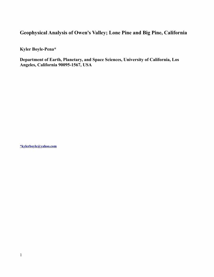
Gravitational data for the Big Pine survey was similarly corrected and modeled, creating the modified data(Figure 9) and the slab model results(Figures 10 and 11).Magnetics - Magnetic surveys were performed at the same survey locations, using a proton procession magnetometer and 3 readings per site. This data was first corrected for drift using the base station magnetometer, then adjusted for a regional correction. The corrected profiles for Lone Pine(Figure 12) and Big Pine(Figure 13) show very noisy profiles, likely due to the proximity to power lines for the majority of the surveys as well as areas containing many buried metal bodies. The profiles could still be modeled using a stepped slab approach similar to the gravity model. These slabs, however, were made up of semi-infinite sheets of dipoles with alternating polarity, and resulted in slightly more complicated models. A reasonable fit could not be made for Big Pine due to noisy data, but the modelinversion and associated geometry can be seen forLone Pine(Figures 14, 15).Seismic Lines – The seismic shot analysis was done using an array of 48 geophones which recorded the travel times and amplitudes of waves generated by a Betsy gun shot. Shots were recorded at each end, as well as a middle shot, in

3

order to analyze the reciprocity between each end. Locations were chosen with hopes of crossing the Lone Pine or Owens Valley fault, where the fault's presence could be confirmed by wave propagation analysis.

The first seismic line was located across a scarp of the eastward dipping Lone Pine fault, where at least 3m of vertical displacement can be seen. Plots of each shot can be seen in figures 16, 17, and 18; each shows the propagation of seismic waves from the east end, middle, and west end of the line. By analyzing the arrival times and wave speeds of the forward and reverse(end) shots, a 2 layer model was created indicating the wave speedof each and the first layer thickness. Figure 19 shows the interpretation for Lone Pine, with a surface layer near 22m thick propagating at 900 m/s and a second layer at 1700 m/s, likely a reflection of water saturated alluvial material of greater consolidation.

Seismic surveys near Goodale road and Tinnemaha were far less conclusive, with no evidence of the fault found at the former and technical difficulties encountered at the former. Goodale Rd. survey indicated slightly faster surface waves and slower second layer waves at a depth of 50m, likely representative of the extremely dry location(Figure 20). The Tinnemahasurvey was conversely done near an active creek, and presented a very shallow surface layer with velocities under 800 m/s and a second layer at 10mdeep of 1800 m/s waves. This again likely representative of the water table, located much more shallow than in the drier locations(Figure 21).

Spectral decomposition of the waveforms was also performed, using a fast fourier transform to calculate the dispersion of the waves. Isolating the dominant frequencies and plotting their phase change produced figure 22, where a wave propagation velocity of 899 m/s was obtained fromthe spatial and temporal frequency plot from one of the Lone Pine shots.Resistivity Survey – Resistivity surveys were performed at the same locations, using a line of 48 electrodes arranged in a Wenner array. Apparent resistivity was measured and used in the software

Res2DInv to create half-space pseudosections representative of relative resistivity. These sectionscan be seen in figures 23, 24, and 25, with the Lone Pine section standing out with visual evidence of the fault. The Lone Pine fault is clearly depicted by the linear interruption of what is likely water saturation.

After this half-space profiling, an apparent resistivity sounding was used for two layer modeling. Data points from electrode configurations centered on the same horizontal location but reflective of different depths were used in the inversion, where a logarithmic plot of resistivity vs. depth is modeled to reproduce the measured values. Characteristic resistivity curves(Figure 26) demonstrate this principal. Using a text-based program compiled through FORTRAN, multiple iterations of the two layer model were run with initial conditions near 1100 and 2400 ohm-m. The averages of the inversion results produced a 13m thick top layer of 1259 ohm-m and a second layer of 2773 ohm-m, thougha large margin of error existed due to the relativelysmaller sample size of logarithmic-spaced data.Self Potential – Self potential measurements were taken at evenly spaced intervals heading west across the Big Pine survey path, using electrodes to measure the existing potential gradient usually generated by conductive ores or water flows. Becuase of the leap frog nature of the survey, an alternating sign cumulative sum is calculated to measure the net change in potential strength. Plotting this path produced Figure 27, showing theincrease is potential as the path is traversed.Magnetotellurics – A magnetotelluric station comprised of two 100m long wires connected to the base recorded data at the Lone Pine campground for three days before being moved to the Tinnemaha campground. By recording electromagnetic data generated mostly by currents in the ionosphere, the data can be used to determine apparent resistivity and corresponding skin depth, particularly the depth to the Mohorovičić boundary(moho).

Magnetic field measured normal to the associated electric field was first corrected to nT

4

by matching the curves to the magnetic base station readings(already in nT). Electric field normal to the magnetic field direction was then converted to volts, and the ratio of E/H was recorded for use in calculation of apparent resistivity and skin depth, using the equation below. The raw plot of this ratio, as well as the calibration effect, can then be seen in figure 28.

Resistivity formula where T is the period and theabsolute value of the ratio is squared.

After filtering the high frequency noise, isolating the dominant longer frequencies allowed for skin depth calculation using the formula:

where ρ is the resistivity as calculated by the previous equation, f is the wave frequency, and μR

is the relative permeability(~1). A plot of skin depth vs. period was then created(Figure 29) and depths of 20-41km to the moho was found for the Lone Pine site, where the large peaks represent theattenuation contrast to the moho. These values come from a small range of large wavelength signals, typically of the order necessary to penetrate through the crust. An average value of 29km was found, a relatively shallow depth for continental crust, though typical with extensional thinning.Broadband Seismics – An earthquake of magnitude 6.4 in the Fiji Islands was recorded using a broadband seismometer installed at the Lone Pine campground; the resulting waveform was analyzed to calculate the depth to the moho.

By isolating the seismometer reading between 2200 and 2250 seconds(the duration of the Fiji earthquake), the transmitted P and S waves, as well as those waves reflected from the moho. Plots of these readings can be seen in figures 30 and 31. Using the program Taup, the distance between our seismometer and the

earthquake epicenter, as well as the arrival times of the first series of seismic waves were calculated.

To determine the wave paths, TauP was used to calculate the spherical ray parameter, a value proportional to the earth's radius and sine of the angle of incidence, and inversely proportional to wave propagation velocity. A value of 4.78 was found using P and S wave velocities of 6400 m/s and 3700 m/s. Using this value, the earth's radius, and an arc length of 86 degrees, arrival times of the initial P waves and reflected waves were calculated and correlated to the broadband data. The crucial number tPS, or the time delay between P and S wave arrival times, will be used in the following equation to determine moho depth:

H is the depth calculated using tPS, ray parameterP, and the square of S and P wave velocities.

The value of tPS was obtained through multiple techniques including receiver functions relying on either deconvolution of the noisy waveforms, or by “rephasing” one of the two normal components to best recreate the other and essentially refining the earthquake generated waveform. The first method attempted required deconvolution of a receiver function with its normal component, producing figure 32 and a tPS value of 3.77s. Further filtering and analysis by cumulative sum of the wave form(Figures 33 and 34) produced similar values of 3.76s and 3.83s(Figures 35 and 36). Rephasing on the the other hand produced the waveform seen in figure 37 and a tPS value of 4.17s.

CONCLUSIONSThe slopes of the Owens Valley fault, as

expected, were found to be steeply dipping to the east as the eastern bounding Inyo faults tended to dip less steeply to the west. The slope of the

5

Alabama Hills block and Owens Valley fault controls much of the western gravity profile and seems to steepen southwards to Lone Pine. Big Pine seems to have a steeper east bounding fault and a shallower Owens Valley fault, or at least a western block less dense than the igneous and metavolcanic rocks of Alabama Hills. Magnetic data from Lone Pine shows a much shallower western boundary, likely a reflection of the relatively less mafic Alabama Hills composition. The major faults of each fault zone within Owens Valley likely run deep to a basal detachment, typical in a zone of expansion. The fault planes and associated zones of weakness likely allowed for the eruption of volcanic rock northwest of Lone Pine and near Big Pine. The two major volcanic areas have differing compositions, also likely evidence refuting the likely hood of a mantle plume.

Surficial surveys produced consistent evidence of typical dry alluvial sediments with wave speeds near 800 m/s covering either water saturated rock or igneous basement rock with speeds ranging from 1600 m/s to 3400 m/s. Of the three short survey locations, only Lone Pine produced clear evidence of faulting. The middle shot of this survey experienced wave speeds 100-150m/s slower than either side shot, a likely reflection of the dry conditions and fault crush zone. The corresponding resistivity survey also produced pseudosections with a clear linear feature right above the fault scarp, a sign of water damming. Results at other sites were less conclusive, with Goodale Rd. survey producing noevidence of faulting and further confirmation of dry horizontal beds. Tinnemaha survey site, located across a creek, heavily reflected the saturated rock in resistivity analysis and experienced difficulties in seismic equipment. SelfPotential produced an increasing voltage as the fault was crossed heading west. This is indicative of increasing water flow as the Sierra Nevadas were approached, expected as water flows down from the mountains. The negative anomaly as the survey path was crossed was like a damming of the water flows, possibly due to faulting.

Magnetotellurics and broadband seismic analysis was performed with the specific goal of determining the depth to the moho, producing values ranging from 23 – 35km. As the broadband results tend to average around 29km, and magnetotellurics suggesting 32 - 36km, the depth to the moho is likely near the low 30s of km. This is within reasonable range for an area of extension and crustal thinning, though as mentioned previously, is likely not shallow enough to reflect an upwelling asthenosphere causing the regional volcanics.

SOURCESBacon, S.N., Pezzopane, S.K., 2007, A 25,000-year record of earthquakes on the Owens Valley Fault near Lone Pine, California; implications for recurrence intervals, slip rates, and segmentation models: Geological Society of America Bulletin July 2007, 119(7-8):823-847 [1] Beanland, S., Clark, M., 1994, The Owens Valley fault zone, eastern California, and surface rupture associated with the 1872 earthquake: U.S. Geological Survey Bulletin 1982, 29 p.

Gans, P.B., Miller E.L., Extension of the Basin andRange Province: Late Orogenic Collapse or Someting Else?. University of California, Santa Barbara, CA. Stanford University, CA. http://www.geol.ucsb.edu/faculty/gans/abstracts/gans1993.html.

Kane, M.F., Pakiser, L.C., Jackson, W.H., 1964. Structural Geology and Volcanism of Owens Valley Region, California – A Geophysical Study. Geological Survey Professional Paper 438, 73 p.

[2]Von Huene, R., Baterman, P. C., Ross, D.C., 1963. Indian Wells Valley, Owens Valley, Long Valley, and Mono Basin. Guidebook for seismological study, 1963 meeting of the International Union of Geodesy and Geophysics: China Lake, California, U.S Naval Ordnance Test Station, p57-110.

6

FIGURES

Figure 1 – Location and fault zones[1]

Figure 2 – Owens Valley cross-section[2]

7

Figure 3 – Magnetic and Gravity survey paths; Lone Pine(south) Big Pine(north)

Figure 4 – Campground, Tinnemaha locations

8

Figure 5 – Seismic and Resistivity survey locations

Figure 6 – Lone Pine gravity profile with terrain correction

9

Figure 7 – Slab model inversion fit

Figure 8 – Geometry of Lone Pine basin

10

Figure 9 – Big Pine corrected gravity profile

Figure 10 – Big Pine model fit

11

Figure 11 – Big Pine basin geometry

Figure 12 – Lone Pine magnetics, corrected for drift

12

Figure 13 – Big Pine mag, corrected

Figure 14 – Lone Pine magnetic model

13

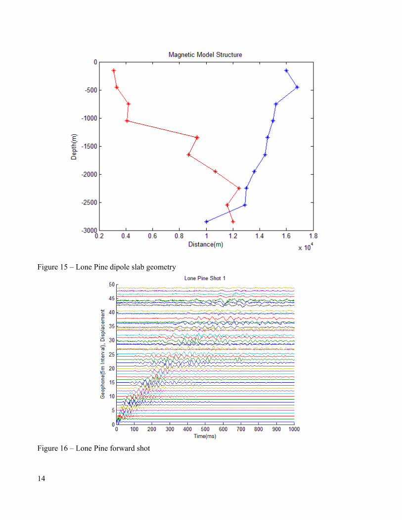
Figure 15 – Lone Pine dipole slab geometry

Figure 16 – Lone Pine forward shot

14

Figure 17 – Lone Pine middle shot

Figure 18 – Lone Pine reverse shot

15

Figure 19 – Lone Pine 2 layer interpretation

Figure 20 – Goodale Rd. 2 layer interpretation

16

Figure 21 – Tinnemaha Campground 2 layer

Figure 22 – Spectral Analysis of all frequencies, upper left contains spectrum of dominant frequencies

17

Figure 23a – Lone Pine resistivity survey

Figure 23b – Lone Pine resistivity surface plot

18

Figure 24 – Goodale Rd. resistivity

Figure 25 – Tinnemaha campground resistivity

19

Figure 26 - Characteristic resistivity curves

Figure 27 – Self potential profile

20

Figure 28 – Lone Pine magnetotellurics calibration, ratio

Figure 29 – LP skin depth vs. resistivity

21

Figure 30 – Broadband north

Figure 31 – Broadband vertical

22

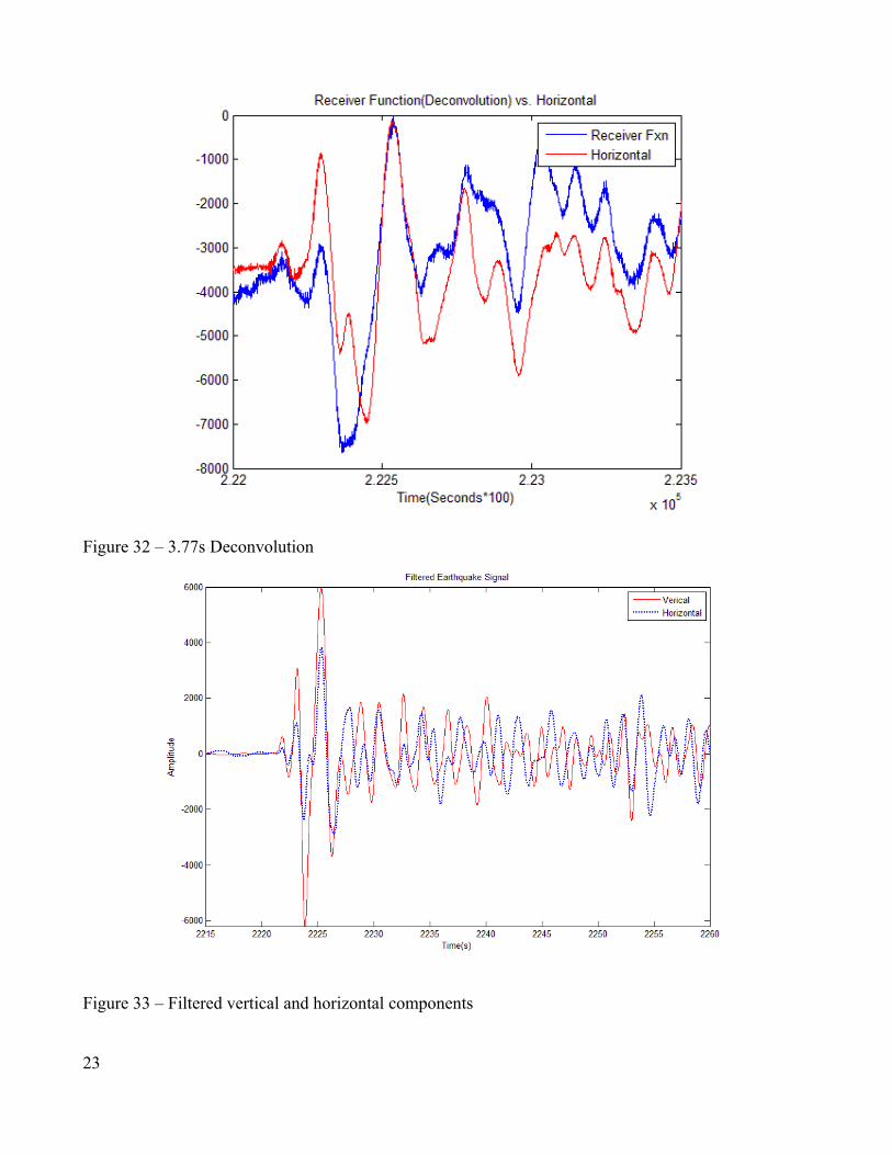
Figure 32 – 3.77s Deconvolution

Figure 33 – Filtered vertical and horizontal components

23

Figure 34 – Filtered cumulative sum

Figure 35 – Alternate horizontal filtering and receiver function

24

Figure 36 – Filtered Vertical component, cumulative sum

Figure 37 – Signal rephasing, tPS of 4.17s

25