WP/14/43

From Volatility to Stability in Expenditure: Stabilization Funds in Resource-Rich Countries

Naotaka Sugawara

© 2014 International Monetary Fund WP/14/43

IMF Working Paper

Research Department

From Volatility to Stability in Expenditure: Stabilization Funds in Resource-Rich Countries

Prepared by Naotaka Sugawara1

Authorized for distribution by Atish R. Ghosh

March 2014

Abstract

This paper examines the effect of stabilization funds on the volatility of government expenditure in resource-rich countries. Using a panel data set of 68 resource-rich countries over 1988–2012, the results find that the existence of stabilization funds contributes to smoothing government expenditure. The spending volatility in countries that have established such funds is found to be 13 percent lower in the main estimation, and similar impacts are found in robustness tests. The analysis also shows that political institutions and fiscal rules are significant factors in reducing the expenditure volatility, while highlighting the roles of the size of economy, diversified exports, real sector management, and financial markets.

JEL Classification Numbers:E62; E63; H10; H50; Q38

Keywords: stabilization fund; fiscal volatility; government expenditure; fiscal policy; institution

Author’s E-Mail Address:NSugawara@imf.org

1 The initial draft of this paper was written, when the author was at the World Bank. The author thanks Salvatore Dell’Erba, Naoko C. Kojo, Keiko Kubota and Mahvash S. Qureshi for helpful comments and suggestions. The findings, interpretations and views expressed in this paper are entirely those of the author and should not be attributed to the IMF, its Executive Board, or its management.

This Working Paper should not be reported as representing the views of the IMF. The views expressed in this Working Paper are those of the author(s) and do not necessarily represent those of the IMF or IMF policy. Working Papers describe research in progress by the author(s) and are published to elicit comments and to further debate.

2

Table of Contents Page

I. Introduction ........................................................................................................................... 3 II. Literature Review ................................................................................................................. 5III. Estimation Strategy ............................................................................................................. 7

A. Empirical Model .............................................................................................................. 7 B. Data .................................................................................................................................. 8 

IV. Results............................................................................................................................... 14V. Sensitivity Analysis............................................................................................................ 15 

A. Alternative Volatility Measures ..................................................................................... 15 B. Different Institutional Indicators and Fiscal Rules ........................................................ 17 C. Restriction of Sample Countries .................................................................................... 19 D. Fixed-Effects vs Random-Effects Models ..................................................................... 20 E. Difference-in-Differences Estimation ............................................................................ 20 

Use of Panel Data............................................................................................................ 21 Two-Period Data ............................................................................................................. 22 

VI. Concluding Remarks ........................................................................................................ 23

References ................................................................................................................................25 Appendix 1: List of sample countries ......................................................................................31 Appendix 2: List of stabilization funds ....................................................................................32 Appendix 3: Definitions and sources of variables ...................................................................33 Appendix 4: Summary statistics ..............................................................................................35 Appendix 5: List of growth acceleration episodes ...................................................................36

Figures

1. The number of countries with stabilization funds – by region and establishment year .....382. Characteristics of stabilization funds, 2009 – by country ..................................................393. Assets of stabilization funds, percentage of GDP, 2009 – by country ..............................404. Trends in the expenditure volatility in countries with and without stabilization funds .....41

Tables

1. Estimation results with discretionary spending volatility ..................................................422. Using alternative volatility definitions ...............................................................................433. Results with different political institutions and fiscal rules ...............................................444. Countries with stabilization funds only .............................................................................455. Results based on fixed-effects or random-effects method .................................................466. Difference-in-differences estimation with panel data ........................................................477. Difference-in-differences estimation with two-period data ...............................................48

3

I. INTRODUCTION

In countries with rich natural resources (e.g., hydrocarbons—oil and gas—and minerals), how to manage revenues collected from them has been one of the major fiscal policy issues. High prices of oil, natural gas and other primary commodities bring a windfall to the governments of the countries with such endowments, which in turn provide the governments with options to use them. Policy makers can strengthen and develop their economies by investing receipts in the areas that contribute to the long-term economic development, such as education and infrastructure. They can also use the receipts to smooth fiscal management, which improves the execution of their growth strategies.

In spite of the benefits that resource endowments could bring, however, many studies (e.g., Sachs and Warner, 2001) have observed that countries rich in natural resources tend to grow more slowly and to have inferior development outcomes than those without. Due to the volatile nature of international prices, dependence on revenue from natural resources tends to cause fiscal volatility and macroeconomic instability. Reducing this dependence is made difficult by the “Dutch Disease,” which is a phenomenon triggered by the production of natural resources attracting large foreign capital inflows, which in turn causes an appreciation of the real exchange rates and weakens the competitiveness of domestic tradable sectors. Non-resource balance of the current account deteriorates, making the economies vulnerable to price swings. In addition, governments of resource-rich economies, especially those lacking strong institutional and legal framework, tend to suffer from the “voracity effect,” which means that a positive shock in government revenues (e.g., revenue windfall from natural resources) results in a more-than-proportional increase in discretionary spending (Tornell and Lane, 1999). This can happen due to a rent-seeking behavior by powerful groups, or policy makers seeking to improve reelection odds by increasing public expenditure. The uncertainty associated with elections also tends to make the incumbent spend more while being in the power. The spending mechanism set up by the current administration could be discarded by the next government (Dixit et al., 2000; and Humphreys and Sandbu, 2007). The increase in spending sometimes takes place in a form of transfers to the private sector, which makes little contribution to overall growth, or in a form that magnifies pro-cyclicality of the economy, which causes further deterioration of the government accounts. As a result, debt accumulates and borrowing costs increase.

To tackle the challenges associated with the use of revenues from natural resources, several countries have introduced stabilization funds—a fiscal instrument to save and set aside a certain amount of revenues for the future when they are needed in stabilizing their economies—since the first establishment in 1953 in Kuwait. Indeed, several definitions of stabilization fund are used in the literature. Balding (2012), for example, defines it as “a government account designed to smooth public expenditures and consumption by setting aside revenue during periods of rapid growth that then could be drawn on during economic contractions” (p. 8). In general, the purpose of stabilization funds, especially in resource-rich

4

economies, is to buffer negative shocks on government expenditure caused by sharp declines in resource prices and the subsequent resource-related revenues.2 Against this background, a key issue is whether or not a stabilization fund works in practice as a cushion to mitigate the fluctuations in government spending. It is often discussed in the literature that having a stabilization fund in itself does not address the issue of expenditure smoothing, so what matters is its design, including clear rules on asset accumulation and investment, and institutional arrangement to enhance transparency and accountability of the fund (e.g., Engel and Valdés, 2000; Bacon and Tordo, 2006; Asfaha, 2007; Le Borgne and Medas, 2007; and Villafuerte et al., 2010). Moreover, in theory, if a resource-rich country maintains sound and appropriate fiscal policy to manage natural resources, the country might not need to establish a stabilization fund to separate the revenue and expenditure cycles. The establishment of stabilization funds is not a requisite to smooth expenditures. Indeed, empirical evidence on the effectiveness of stabilization funds on fiscal policies in general, and expenditure volatility in particular, is rather inconclusive (e.g., Devlin and Lewin, 2005; and Barma et al., 2012). The main objective of this paper is to examine if the presence of stabilization funds helps the governments in resource-rich countries reduce their expenditure volatility. The analysis shows that government expenditure is found to be less volatile in countries that have stabilization funds. The estimation result based on the main specification indicates that the volatility of government spending in countries with stabilization funds is 13 percent lower than that in countries without such funds. In most cases, robustness tests also show the negative relationship between the presence of stabilization funds and the spending volatility. The impacts are found to be around 15 to 20 percent. This paper contributes to the existing literature in several ways. First, unlike previous studies on stabilization funds, as reviewed in detail in the next section, the impact of stabilization funds is assessed with other potential factors of expenditure fluctuations taken into account. Second, this paper makes good use of different indicators, specifications and estimation methods in analyzing the role of stabilization funds. This is made possible by the use of a panel data set consisting of 68 resource-rich countries over a 25-year period. Third, as the flip side of the first point, this paper provides additional evidence of determinants of the expenditure volatility to the relevant literature. It covers a wide range of indicators, for 2 Nowadays, stabilization funds are normally treated as a type or function of Sovereign Wealth Funds (SWFs), and thus, can be recognized as SWFs whose purpose is stabilization of the economies. Although the definitions of SWFs vary, as in the case of stabilization funds, generally speaking, SWFs are government investment (or saving) funds to manage foreign assets and invest them for earnings (e.g., Aizenman and Glick, 2009; and Sun and Hesse, 2010). The IMF (2012a) uses the definition in the Santiago Principles and classifies 30 SWFs where the data are publicly available into four types: (1) stabilization funds, (2) pension reserve funds, (3) reserve investment funds, and (4) saving funds. For the Santiago Principles, refer to the web site of the International Forum of Sovereign Wealth Funds (IFSWF) at http://www.ifswf.org.

5

instance, the ones related to economic structure, real sector management and financial markets. The rest of the paper is structured as follows. Section II reviews the existing literature that explores the relationship between stabilization funds and their impacts on fiscal conditions, mainly focusing on the works with quantitative assessment in the macroeconomic context. Section III explains the data and empirical methodology employed in this paper. Section IV presents the main results of the analysis on the expenditure volatility. Section V discusses and reports the results of robustness tests. Finally, Section VI concludes.

II. LITERATURE REVIEW

The existing empirical evidence on the association between stabilization funds and fiscal outcomes is rather mixed. Some studies focus on a single country or handle multiple countries separately, while some examine the impact of stabilization funds using a cross-country data set. As a study in the former category, Fasano (2000) reviews natural resource funds in five countries—Norway, Chile, Venezuela, Kuwait, and Oman—and one U.S. state (State of Alaska). The study finds that the effects of the funds on fiscal management vary by country or, in other words, by objective of the funds. The author shows that while stabilization funds tend to help in strengthening the effectiveness of fiscal policy by separating expenditure from the revenue availability, they cannot be substituted for sound fiscal management. The paper emphasizes that the successful stabilization schemes are related to governments’ commitments to fiscal discipline and good macroeconomic management. Most countries reviewed in Fasano (2000) are also examined in Davis et al. (2001), which use Chile, Kuwait, Norway, Oman and Papua New Guinea, as well as seven resource-rich comparator countries. The study examines the impact of the establishment of funds on government spending. Employing time-series analysis and structural break tests, it finds that government expenditure tends to be less correlated with changes in resource export receipts in countries with resource funds than in those without, though the relationship is not uniform. It also shows that the establishment of funds does not have a significant impact on government spending, and suggests that the causal relationship is reverse, meaning that countries with more prudent expenditure policies tend to establish stabilization funds. The stabilization fund in Venezuela is examined in Clemente et al. (2002). It assesses how effective the stabilization fund is in reducing the macroeconomic volatility, including the government revenue volatility, using a dynamic computable general equilibrium model. In addition to the actual stabilization fund the country has, the study uses two alternative/hypothetical funds based on different fund designs (e.g., sizes of the fund and the deposits into the fund) and compares the results between different scenarios. The authors show that, with the positive oil price shocks, the actual stabilization fund does not perform well in reducing the volatility but the hypothetical ones work. On the other hand, both actual

6

and alternative stabilization funds perform well in reducing the volatility when faced with negative oil price shocks, though the latter are still more effective. In the meanwhile, Merlevede et al. (2009) show that the introduction of the oil stabilization fund in Russia mitigated economic fluctuations caused by the oil price shocks. Using a dynamic open macroeconomic model based on the data over the period of 1995–2007, it shows that Russia’s economic prosperity during the sample period is due to the increasing oil price. The paper also highlights that the economy is vulnerable to negative shocks in oil prices and private sector confidence. The authors argue that such negative shocks can be eased by changes in fiscal policies, namely, taxation and stabilization fund. The following studies are based on a panel data, and therefore, are more related to the purpose of this paper. Crain and Devlin (2003) construct a data set covering 71 countries over the period of 1970–2000 and show that natural resource funds increase fiscal volatility, particularly in oil-exporting countries. Using the volatility of government expenditure and controlling for economic and demographic factors, the authors show that the presence of nonrenewable resource funds raises the volatility. However, when they focus on the three oil-exporting countries with natural resource funds (i.e., Chile, Norway and Oman), the study finds that the expenditure volatility was reduced after the establishment of funds in Chile and Norway. The authors argue that the mixed results are because of differences in the fund management rules and savings and investment decisions, as well as overall fiscal policy framework. Ossowski et al. (2008) examine the effects of fiscal institutions (oil funds and fiscal rules) on fiscal outcomes using the data over the period of 1992–2005 for oil-producing countries. The study employs three measures as fiscal outcomes (i.e., non-oil primary balance, growth in government expenditure and ratio of changes in expenditure and oil revenue) and concludes that the fiscal outcomes are not due to the introduction of oil funds and fiscal rules. In their regression estimations, the authors find that the presence of fiscal institutions has a negative, but statistically insignificant, effect on non-oil primary balance and a positive relationship with expenditure growth. What the study finds is the importance of governance institutions (e.g., government stability, corruption, etc.). Higher institutional quality is associated with higher non-oil primary balance, and lower correlation between expenditure and revenue, which suggests that countries with higher quality institutions are able to overcome the “voracity effect.” Finally, Bagattini (2011) first looks at each of 12 countries that have stabilization funds separately and then estimates the impact of the funds using a panel data. Using the data over the period of 1992–2007, the author creates an indicator that measures the success of stabilization funds, based on six fiscal variables (level and change in overall fiscal balance, level and change in non-resource fiscal balance, and changes in non-resource revenue and public debt). The study finds that only one country shows a decrease in the “success” value

7

(i.e., worse fiscal performance) after the establishment of stabilization fund. The analysis with the panel data confirms that the presence of stabilization funds is positively related to non-resource fiscal balance and reduces public debt. The estimation results also show that the political stability and the rules of the funds are important factors for success.

III. ESTIMATION STRATEGY

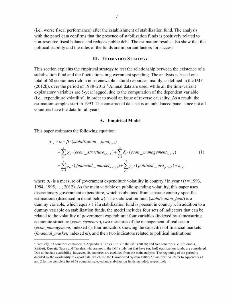
This section explains the empirical strategy to test the relationship between the existence of a stabilization fund and the fluctuations in government spending. The analysis is based on a total of 68 economies rich in non-renewable natural resources, mainly as defined in the IMF (2012b), over the period of 1988–2012.3 Annual data are used, while all the time-variant explanatory variables are 5-year lagged, due to the computation of the dependent variable (i.e., expenditure volatility), in order to avoid an issue of reverse causality. As a result, the estimation samples start in 1993. The constructed data set is an unbalanced panel since not all countries have the data for all years.

A. Empirical Model

This paper estimates the following equation:

, , 5

4 2

, , 5 , , 51 1

4 2

, , 5 , , 5 ,1 1

( _ )

( _ ) ( _ )

( _ ) ( _ ) ,

i t i t

s s i t v v i ts v

m m i t p p i t i tm p

stabilization fund

econ structure econ management

financial market political inst

(1)

where σi,t is a measure of government expenditure volatility in country i in year t (t = 1993, 1994, 1995, …, 2012). As the main variable on public spending volatility, this paper uses discretionary government expenditure, which is obtained from separate country-specific estimations (discussed in detail below). The stabilization fund (stabilization_fund) is a dummy variable, which equals 1 if a stabilization fund is present in country i. In addition to a dummy variable on stabilization funds, the model includes four sets of indicators that can be related to the volatility of government expenditure: four variables (indexed by s) measuring economic structure (econ_structure), two measures of the management of real sector (econ_management, indexed v), four indicators showing the capacities of financial markets (financial_market, indexed m), and then two indicators related to political institutions 3 Precisely, 63 countries contained in Appendix 1 Tables 1 to 3 in the IMF (2012b) and five countries (i.e., Colombia, Kiribati, Kuwait, Nauru and Tuvalu), who are not in the IMF study but that have (or, had) stabilization funds, are considered. Due to the data availability, however, six countries are excluded from the main analysis. The beginning of the period is decided by the availability of export data, which use the Harmonized System 1988/92 classification. Refer to Appendices 1 and 2 for the complete list of 68 countries selected and stabilization funds included, respectively.

8

(political_inst, indexed p). Finally, α is a constant term and εi,t is an error term for country i in year t. As the main estimation technique, this paper uses ordinary least squares (OLS) with panel-corrected standard errors (Beck and Katz, 1995). By employing this estimation method, standard errors are corrected for heteroskedasticity and contemporaneous correlation across countries. In other words, it is assumed that, in the estimation of variance-covariance matrix, each country has its own variance and each pair of countries has different covariance. The technique of using a panel-corrected standard error calculation is used by Desai and Kharas (2010) and Albuquerque (2011) in a specification where the dependent variable is estimated country by country, as this paper does. The use of OLS, rather than other panel estimation methods, especially fixed-effects model, can be also justified by the fact that the variable of interest is binary and remains unchanged in most of the samples—even if changed, it seldom changes again. Still, in order to mitigate the risk of omitted variable bias and check for robustness of the results, specifications with additional explanatory variables, especially country-specific characteristics that are not or little changed over time and that are related to the quality of institutions, are tried. Furthermore, as a part of robustness tests, this paper employs fixed-effects (or, random-effects) and difference-in-differences methods to examine whether the results from the main specification hold with different estimation methods.

B. Data

In estimating Equation (1) and measuring the impact of stabilization funds on the government spending volatility, multiple data sources are used. The definitions, constructions and sources of data used in this paper are presented in Appendix 3. Volatility of government expenditure (dependent variable). As mentioned above, this paper employs discretionary government spending, which is obtained through country-specific regression estimations. Building on the method used by Fatás and Mihov (2003 and 2006), this paper estimates: , , , 1 ,ln( ) ln( ) ln( ) ,i t i i i t i i t i i i tG Y G Z (2)

where Gi,t and Yi,t are real general government expenditure, deflated by GDP deflator, and real GDP in country i in year t, respectively. The equation also includes real government expenditure in the previous year (t-1) and a set of control variables, Zi. The control variables consist of inflation in year t, average hydrocarbon price indices in years t and t-1 (expressed in logs), which are computed from coal price in Australia, crude oil price in Dubai and natural gas prices in the United States and Europe. The constant for country i is αi and νi,t is an error term for country i in year t. By estimating Equation (2), the effect of business cycle is excluded and the equation yields country-specific discretionary component of government expenditure as the residual, νi,t. The

9

estimation is done country by country, using the data over the period of 1980–2012.4 The instrumental variables (IV) estimation method is employed to address the possible problem of reverse causality going from the current real government expenditure growth, Δln(Gi,t), to real output growth in the same year, Δln(Yi,t). Adopting the strategy often used in the literature (e.g., Herrera and Vincent, 2008; Furceri and Poplawski Ribeiro, 2008; Afonso et al., 2010; and Brzozowski and Siwińska-Gorzelak, 2010), it uses the following indicators as instruments for current real GDP growth: two lagged values of output growth (t-1 and t-2), lagged inflation (t-1), lagged government expenditure growth (t-1), and hydrocarbon price index in year t. Finally, the volatility is measured as the log of 5-year moving standard deviation of the residuals from the IV estimation using values in years from t-4 to t. Presence of stabilization fund (stabilization_fund). The effect of stabilization funds is captured by a dummy variable taking a value of 1 if a stabilization fund exists in a given year. For the sake of simplicity, it is assumed that the operation of the fund starts in the following year. For example, if the establishment year of stabilization fund in country i is 2000, the dummy takes the value of 0 for t = 2000, but 1 for t = 2001. In equation (1), values in year t-5 are used. The choice of 5-year lagged values is potentially important, since this paper looks at the volatility of government spending after the establishment of stabilization funds (i.e., years t-4 and onward). The binary variable is used due to the lack of detailed time-series information (e.g., financial assets and liabilities) on stabilization funds, but this is an approach often employed in the literature (e.g., Shabsigh and Ilahi, 2007; and Ossowski et al., 2008). This paper relies on multiple sources for the definition of stabilization funds and their establishment years.5 It should be noted that this paper uses the establishment years. In some cases, there is a gap between the years stabilization funds are established and the ones these funds actually start operating (e.g., transfer of money from/to fund accounts).6 As a result, this paper covers 32 countries that have—or, had if already abolished—stabilization funds. The number of funds considered in this paper is 37, since countries can have more than one fund. If multiple stabilization funds exist in a given country, the year when the first fund was established is used in creating the dummy variable. The basic characteristics of these funds are presented in Figures 1–3. 4 The individual estimation results are available from the author upon request. It is also examined whether or not the residual from Equation (2) is correlated with the stabilization fund dummy in Equation (1). In so doing, the interaction term between output growth and the stabilization fund dummy, as well as the dummy variable itself, is added to Equation (2). Then, the coefficient of output growth from this modified equation and the one from Equation (2) are compared, in order to check if stabilization funds affect output growth directly. Except for Azerbaijan, no major changes in the magnitude of coefficient are found.

5 The following literature is mainly used to identify stabilization funds: IMF (2008, 2010 and 2012b), Ossowski et al. (2008), UNCTAD (2008), Truman (2009 and 2010), Kojo (2010), Kunzel et al. (2010), Sinnott et al. (2010), Bagattini (2011) and Baunsgaard et al. (2012). The list of stabilization funds included in this paper is in Appendix 2.

6 One example is Norway. As defined in this paper, the country created a stabilization fund in 1990 but the transfer started in 1995. Also, as discussed in Kalyuzhnova (2006), the accumulation of assets (with no spending) was required for the initial five years in the stabilization funds in Azerbaijan and Kazakhstan. It would be desirable to use the years when funds start actually working, but such information is not available in a consistent manner for many of them.

10

In Figure 1, all 32 countries that have ever created stabilization funds are grouped by geographical region and by establishment year (of the first fund). It shows that the funds can be found all over the world. Half of them (16 countries) created their (first) funds after 2000, and there are some region-specific trends in establishing the funds. First, most of the funds in the Asia and the Pacific region, especially in Pacific island economies, were created before 1980, while many funds in Africa and Central Asia (which is a part of MCD) are relatively new (i.e., created in the 2000s). Second, only the Middle East region created new stabilization funds in all four periods. Finally, the fund establishment in Western Hemisphere is concentrated in the 1990s (only one in the 1980s), which is likely to be related to structural adjustment programs endorsed by the IMF and the World Bank (e.g., Arrau and Claessens, 1992; and World Bank, 2003). Figure 2 shows scores of the 2009 version of Sovereign Wealth Fund (SWF) scoreboard for 18 countries with stabilization funds where data are available (Truman, 2010).7 The scoreboard considers four areas of SWF characteristics, namely, structure, governance, accountability and transparency, and behavior, and scores them using 33 questions. In Figure 2, each of the four categories is adjusted to have an equal weight, with the overall maximum possible score of 1 (i.e., 0.25 is assigned to each area). The overall scores range from 0.16 for Sudan to 0.94 for Norway, with the rest of the observations evenly distributed. The areas that differentiate stabilization funds are not the fund structure, but governance (i.e., roles of government/governing bodies and fund managers, as well as ethical guidelines) and, to a lesser extent, transparency and accountability to citizens and governments on their investment strategies. Most countries (or stabilization funds) in Figure 2 have scores in the structure category close to the maximum, while their governance scores vary widely. Norway is the only country whose score in the governance area is above 90 percent of the maximum score (i.e., more than 0.225). It is joined by Timor-Leste and Trinidad and Tobago for the accountability and transparency score. Figure 3 presents each stabilization fund’s assets under management as in mid-2009 or most recent date, which is also taken from Truman (2010). The numbers are expressed as a percentage of each country’s GDP in 2009. The percentage shares range from more than 300 percent for Kiribati and Tuvalu to less than 0.5 percent for Sudan and Venezuela. The amounts in billions of US dollars are included in the parentheses next to the respective country names. The assets-to-GDP ratios in Pacific island countries are quite high, while the amounts themselves are relatively small. This means that those funds might not be key players in the international financial market, but play important roles in their domestic economies. The stabilization funds in Western Hemisphere and in African countries tend to 7 Although it is possible that two and more stabilization funds are included in a country in Figures 2 and 3, only one fund is identified per country.

11

be relatively small both internationally and domestically. The opposite trend can be shown in the funds in Middle East and Central Asia, which are large players both internationally and domestically. Economic structure (econ_structure). This paper controls for the economic structure, as they are likely to be associated with the government expenditure volatility. The first variable is the government size, measured by log of general government expenditure as a percentage of GDP in year t-5. Bigger governments tend to have larger automatic stabilizers, and as a result, need fewer discretionary components in adjusting expenditure. Therefore, their expenditure tend to be less volatile (Fatás and Mihov, 2001; Debrun et al., 2008; and Afonso et al., 2010). The size of government is expected to be negatively related to the expenditure volatility. The second indicator is the size of the economy, measured by the initial level (i.e., lagged 5 years) of total population (in logs). Furceri and Karras (2007) and Furceri and Poplawski Ribeiro (2008) find the government expenditure volatility to be negatively related to the size of economy, since smaller economies are more exposed to economic shocks and more volatile, and hence, their governments tend to spend more to absorb shocks. Also, larger countries tend to have broader revenue bases spread among larger number of taxpayers, which helps to reduce volatility of both revenue and expenditure (Furceri and Poplawski Ribeiro, 2008). As the third indicator to capture the economic structure, the level of development, PPP-adjusted real per capita GDP, is included. It is expected that countries with higher income level (i.e., more developed) can manage public spending better (i.e., less volatile expenditure). 5-year lagged values are used. The last variable related to the economic structure of resource-rich countries is an index of export product diversification, which is measured by Theil’s entropy index. It measures “equality” of the country’s export basket, with a lower number indicating more equality (i.e., export products are more diversified). The index is computed by:

, , , ,,

1, , ,

1ln ,

nk i t k i t

i tki t i t i t

x xT

n

where .

1

1,,

,,

n

ktik

titi x

n (3)

Ti,t is Theil’s entropy index for country i in year t, where xk,i,t represents the amount of product k exported by country i in year t, and ni,t is the number of total export lines in country i in year t. The calculation is based on the 6-digit-level export data classified by the Harmonized System 1988/92, obtained from the UN Comtrade database. Due to the data availability, the mirror data (i.e., import statistics from the partners, rather than the export amounts by reporters) are used. Resource-rich countries that are dependent on a smaller number of export products might experience larger volatility of government expenditure.

12

Countries whose export product indices are “less equal” tend to concentrate on exporting natural resources or products highly dependent on raw materials, and their export receipts are affected more by changes in the international prices. This, in turn, may oblige the government to spend more on export subsidies or take other measures to mitigate negative effects of the price fluctuations. Economic management (econ_management). The second set of control variables is related to the management of the economy, specifically, output volatility and inflation. The first is defined as the 5-year moving standard deviation of annual real GDP growth. The relationship between government expenditure volatility and output volatility is expected to be positive (e.g., Hakura, 2009) because the volatility of economic activities requires governments to adjust their expenditure more widely. The initial level, year t-5, is used. The variable on inflation is measured by the log difference of consumer price index (CPI) from the previous year, expressed as a percent, in year t-5. As in Agnello and Sousa (2009), higher inflation is expected to lead to more expenditure volatility, as the fiscal policy formulation is made more difficult by the higher level of economic uncertainty. In order to avoid undue influence by outliers, the cases of extremely high inflation rates are transformed using the method used in Ghosh et al. (2005). Financial market (financial_market). Financial markets may affect government expenditure volatility as they may function as a source of expenditure smoothing. This paper distinguishes between domestic and international financial markets, and uses one indicator from the former and two from the latter. For the first, it uses liquid liabilities, defined as the broad money as a share of GDP. The level and the volatility (i.e., the log of 5-year rolling standard deviation) of this indicator are included in order to measure not only the depth of domestic financial market, but also its stability. Deep and stable domestic financial market can contribute to reducing the spending volatility, and hence, spending volatility is expected to have a negative relationship with the level of liquid liabilities and a positive one with financial market volatility (Herrera and Vincent, 2008). As the first variable related to the international financial market, a measure of physical accessibility is used. It is measured by the distance to the closest major financial center (London, New York or Tokyo), taken from Rose and Spiegel (2009). This international financial remoteness is measured by great-circle distance and time-invariant. Countries far from financial centers tend to face more difficulty accessing international financial resources, and are less capable of using them to reduce the expenditure volatility. Therefore, the distance is expected to be positively related to the government expenditure volatility. In addition to the measure of physical access to the international financial market, this paper adds an index of capital account openness to see how the degree of financial openness affects the volatility of government spending. As in the financial remoteness measure, countries

13

more financially open can have more options to mitigate the effect of volatile expenditure. At the same time, different from the simple location measure, economies with a more open capital account could face more volatile government expenditure in order to handle the fluctuation of capital flows. Therefore, the sign of this indicator could be either way. The index of financial openness is taken from Chinn and Ito (2006), updated in April 2013. Political institution (political_inst). The last set of control variables is the quality of political institutions, as their importance in the course of economic development has been emphasized by many studies (e.g., Acemoglu et al., 2003; and Klomp and de Haan, 2009). It is measured by an index of “political freedom,” computed from two indices in Freedom in the World 2013 (Freedom House). The index is defined as a simple average of “political rights” and “civil liberties,” ranging from 1 to 7, with higher values indicating less freedom. Countries with stronger political institutions are more likely to limit the discretionary spending by policy makers, and as a result, tend to have less volatile fiscal policy (Henisz, 2004). This indicator is chosen mainly because of the wide coverage in both time and country dimensions. Since this paper is interested in resource-rich countries since 1988, not many databases fit well with this purpose. Several well-established databases, such as the Worldwide Governance Indicators (Kaufmann et al., 2010), have institutional indicators for a number of countries but the time coverage is limited. In the same vein, there are some databases (e.g., International Country Risk Guide—ICRG) in which long time-series data are available, but the country coverage is less desirable for the purpose of this paper. As a part of robustness tests, alternative variables of political institutions from different data sources are tried. It also includes other time-invariant country-specific components that are considered to be related to the government quality (e.g., legal origins and geographical characteristics). The second variable for political institutions is an interaction term between the political institutions and the stabilization fund dummy (stabilization_fund). By adding the interaction term to the equation, the effects of political institutions on expenditure volatility for countries with and without stabilization funds are differentiated. It is expected that the quality of political institutions is even more important in countries with stabilization funds in reducing the volatility. Countries with stabilization funds have more scope for increasing public spending during commodity booms, which weak political institutions (e.g., unaccountable governance structure and non-democratic political system) would fail to curtail. On the other side of coin, effective fund management by the administration governed by strong institutions can make a sizable contribution to stability of expenditure.

14

IV. RESULTS

Table 1 presents the estimation results using the volatility of discretionary government expenditure as the dependent variable.8 In addition to the specification with all the explanatory variables presented in column 7, the table also shows the regression results with different combinations of right-hand-side variables, in order to check if the results are unduly affected by them. In the specifications without the interaction terms (i.e., columns 1–4), the coefficients of the stabilization fund dummy have a negative sign. This relationship is statistically significant at the 1 percent and 5 percent levels. It is found that the establishment of stabilization funds in resource-rich countries is associated with the reduction in the expenditure volatility. Everything else being held constant, the volatility of government expenditure in countries with stabilization funds is 13 percent lower than that in countries without funds (column 4). The four variables capturing the economic structure also have the expected signs and are mostly statistically important. The larger the government size and the more populous the country, the less volatile the government spending tends to be. Across all the specifications, the latter (i.e., population) is found to be statistically significant and a one-percent increase in the population size is associated with an around 0.15 percent decrease in the expenditure volatility. The income level is also important in lowering the public spending volatility, though it is not always significant. Export product diversification is related to stable government expenditure, and the relationship is found to be strong as in the case of the population size. It shows that a one-point decrease in the equality index (i.e., more diversified export product baskets)—roughly saying, corresponding to a change in the index from the 75th percentile to the median—reduces the volatility by around 4 percent. The coefficients of the variables measuring management of the real sector are positive, as expected, and statistically significant. Output growth volatility and high inflation in the initial years increase the government fiscal volatility, and the relationship is quite strong. A one percent increase in the volatility of output growth raise that of government expenditure by 0.15 percent, while a one percentage-point positive change in inflation is related to an increase in the volatility by around 0.5 percent. In the meanwhile, domestic and international financial markets act as buffers to smooth public expenditure. The domestic financial depth reduces the volatility of government expenditure, while the volatility of domestic financial market increases the spending 8 There are six countries excluded from the estimations due to the data availability. Half of them are those who have stabilization funds: Nauru, Timor-Leste and Tuvalu, while the remaining three countries are Afghanistan, Brunei Darussalam and Iraq. The summary statistics of variables used in the main estimations and robustness tests are presented in Appendix 4.

15

volatility. The accessibility to international financial centers and the openness of capital account are also related to less volatile government spending. For instance, when the domestic financial market becomes more volatile by one percent, the volatility of government expenditure is increased by around 0.06 percent. Finally, better institutional quality is associated with lower expenditure volatility. The relationship is always statistically significant and is found to be strong. The interaction term with the stabilization fund dummy has the same sign as the institutional quality does, and, again, statistically significant. That is, weaker political institutions are found to be associated with higher government expenditure volatility in countries with stabilization funds, compared to those without. In other words, the relationship between worse institutional environment and more volatile government expenditure is found to be stronger in countries with stabilization funds. For those who do not have stabilization funds, an increase in the political freedom score (i.e., institutions are weakened) by one unit (i.e., a change from the 10th to 25th percentiles in the index score) leads an around 4 percent increase in the government expenditure volatility.9 Under this circumstance, if a country has a stabilization fund, the country is likely to face an additional increase in the volatility by 4 percentage points.

V. SENSITIVITY ANALYSIS

This section conducts tests to check the robustness of the results presented in the previous section, especially to examine whether or not the effect of the establishment of stabilization funds would hold under alternative specifications. The check is done in five different ways. The first three sets of tests are related to the use of different indicators and samples: the specifications (A) introducing alternative indicators of government expenditure and a measure of cyclically-adjusted fiscal balance (CAFB) to compute the dependent variable (Table 2), (B) employing different institutional indicators and time-invariant measures such as legal origins and geographical characteristics, as well as those related to fiscal rules (Table 3), and (C) restricting the samples to only those with stabilization funds (Table 4). In the other two sets, different estimation methods are tried, namely, (D) fixed- or random-effects method (Table 5) and (E) difference-in-differences estimation (Tables 6 and 7).

A. Alternative Volatility Measures

The first set of robustness tests is carried out with three different expenditure measures as well as a fiscal balance adjusted for the cyclical effects (Table 2): real overall general government expenditure growth (columns 1 and 2), growth in real public investment (columns 3 and 4), real public consumption expenditure growth (columns 5 and 6), and CAFB as a share of potential GDP (columns 7 and 8). The volatility of these four indicators 9 In the estimation sample, Chile and Madagascar in early 2000s are at the 10th and 25th percentiles of the distribution in the political freedom score, respectively.

16

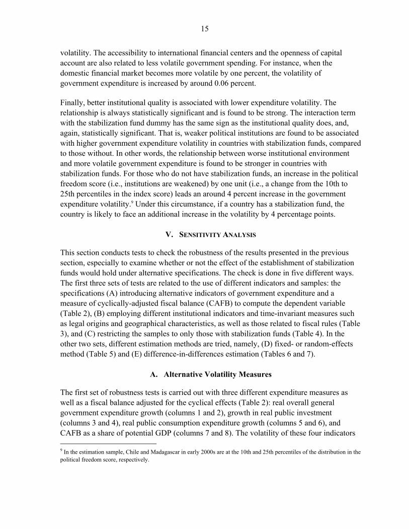
is defined as 5-year moving standard deviation, based on years from t-4 to t, as in the discretionary government expenditure. They are used as the log in order to handle the effects of outliers. The data on overall government expenditure and public investment are taken from the IMF World Economic Outlook. The series of government consumption expenditure is also obtained from the IMF World Economic Outlook, but supplemented by the data from the World Bank World Development Indicators for countries whose data are not available in the IMF database. CAFB (in country i in year t) is computed with data from the IMF World Economic Outlook and simply defined by:

,, , ,

,

,p

i ti t i t i t

i t

YCAFB GREV GEXP

Y

(4)

under the assumption that elasticity of overall revenue, GREV, and overall expenditure, GEXP, is one and zero, respectively. Y and Yp are, respectively, actual and potential levels of GDP, and the latter is obtained by the Hodrick-Prescott (HP) filter with the smoothing parameter of 6.25. Since the first three volatility measures based on government expenditure are not adjusted for the cyclical effects, estimations using these volatility variables focus on the boom periods only (i.e., columns 1 to 6). Government expenditure can be increased when countries are in recessions or crises in order to pull their economies up, which, in turn, results in an increase in the volatility during such periods (if using cyclically-unadjusted data). In countries with stabilization funds, money set aside during the high growth years is released to spend more to recover from the economic contractions. Hence, it is probably appropriate to focus only on the periods of high growth in the estimation analysis based on non-adjusted volatility measures. The boom periods are identified using the framework of growth acceleration developed by Hausmann et al (2005). Following the empirical literature (e.g., Fabrizio et al., 2009; and Berg et al., 2012), the series of real GDP is used to find growth acceleration episodes. Specifically, an episode starts when (1) the average annual real GDP growth rate over the following 5 years is more than or equal to 3.5 percent and (2) a difference in the average annual GDP growth rates between the previous 5 years and the following 5 years is at least 2 percentage points. The episode ends when (1) the average annual growth rate over the next 5 years is less than or equal to 2 percent and (2) annual growth of the following year is below 3 percent. The end of acceleration episodes is also found when (3) negative GDP growth is recorded. Finally, any episodes that continue less than or equal to 3 years are dropped. The GDP series is taken from the IMF World Economic Outlook and includes projections in later years, so as to cover the period of 1980–2013. The growth acceleration episodes are reported in Appendix 5.

17

The estimation results using the main specification including and excluding the interaction between the stabilization fund dummy and political institution (i.e., columns 4 and 7 in Table 1) are presented in Table 2 and are similar to those in Table 1. There are 57 countries included in columns 1 and 2 and fewer countries are in columns 3 to 6, due to the identification of growth acceleration and data availability. In the meanwhile, estimations with CAFB in columns 7 and 8 are based on the same samples as in Table 1. Focusing on the coefficients of the stabilization fund dummy, the institutional quality and their interaction term, the table shows that the presence of stabilization funds has a negative and significant effect on consumption expenditure volatility (column 5) as well as the volatility of CAFB (column 7). In countries without stabilization funds, on average, CAFB is found to be 20 percent more volatile than in countries having them. It also shows that political freedom is a significant determinant of expenditure volatility in the three unadjusted expenditure series. Regarding the interaction, the coefficients of all volatility indicators but a measure of overall expenditure are found to be statistically significant, and their signs are expected. Weak political institutions are more associated with volatile government expenditure in countries with stabilization funds than in those who do not have them.

B. Different Institutional Indicators and Fiscal Rules

In Table 3, the results of regressions run with different institutional indicators are presented. While the table shows coefficients of the stabilization fund dummy and institutional indicators, all the estimations are carried out with other determinants of expenditure volatility (i.e., columns 4 and 7 in Table 1). Panel A of the table introduces two different measures of political institutions. The first alternative institutional variable is the indicator of political regime, a measure taken from the Polity IV Project, ranging from -10 (strongly autocratic) to 10 (strongly democratic). Fewer countries are covered by this indicator than by the Freedom House measure, but the longer time-series data are available. The second alternative is the sub-soil resource rents, expressed as a percentage of GDP, as a proxy of political discretion related to the resource management.10 Sub-soil resource rents are defined as a sum of rents from oil, natural gas, coal and minerals, which are obtained from the World Bank World Development Indicators. This paper also examines the role of fiscal rules in reducing the government expenditure volatility (Panel B). The data on fiscal rules are from the IMF Fiscal Rules Dataset 2013 (Schaechter et al., 2012), updated in September 2013. The database has the detailed information on fiscal rules by type—budget balance, debt, revenue and expenditure—and by 10 For the discussion on the relationship between resource rents and institutions, refer to, among others, Collier and Hoeffler (2009), Arezki and Brückner (2011), and Bjorvatn et al. (2012). The literature on natural resources and development, including the discussion of rents is reviewed in van der Ploeg (2011).

18

level (national and supranational) since 1985. Although it covers a total of 87 countries, the information is available for only 21 countries considered in this paper. Due to the limited number of samples, it uses all types of fiscal rules, rather than focusing on the rules related to revenue and expenditure. Specifically, two indicators are employed. The first one is the total number of rules in place. Since this measure shows an aspect of the quantity only, this paper computes an index of the strength of fiscal rules, following IMF (2009) and Schaechter et al. (2012). The index is based on the principal component analysis using different characteristics of rules: (1) monitoring of compliance outside government, (2) formal enforcement procedure, (3) coverage, (4) legal basis, (5) well-specified escape clause and (6) supporting procedures/institutions. First, six sub-indices are computed for these six characteristics, by aggregating individual scores for all types and levels of rules by characteristic and then dividing by the maximum possible score.11 Then, the principal component analysis is conducted using these six sub-indices. The final score is standardized, which average value is zero and standard deviation is set one, showing the higher the values, the more strengthened the fiscal rules are. In addition, three time-invariant indicators are included—legal, latitude and location, as presented in the tables. “Legal” is the legal origin and taken from La Porta et al. (1999). There are five types of legal origin—British, French, German, Scandinavian and Socialist—and each country belongs to one of these legal systems.12 Rose and Spiegel (2009) are the source of the other two indicators, “latitude,” which is the absolute value of the latitude from the equator, and “location,” which are two dummy variables for landlocked and island countries. For countries where the latitude information is missing, data are obtained from Mayer and Zignago (2011). The World Factbook 2013 by the Central Intelligence Agency (CIA) of the United States is also used as an additional source of information on location. As the fourth measure, it considers an indicator that is almost time-invariant: presidential system. The measure is a dummy variable taking a value of 1 if the government structure is based on the presidential system. The information is taken from the Database of Political Institutions 2012, updated January 2013 (Beck et al., 2001). The CIA World Factbook 2013 is also used for countries the information is not available in the database. In column 1 in Panel A, it is shown that the use of latitude, dummy variables for landlocked and island countries and legal origin dummies, instead of political freedom, does not affect the estimation results of stabilization fund dummy. The dummy variable is still negative and statistically significant at the 1 percent level. In columns 2 and 3, all the time-invariant factors (including a dummy on presidential system) are added to the main specification (i.e., 11 In coverage and legal basis, individual scores are first rescaled to range from zero to one. For supporting procedures/institutions, an index is first computed using three components related to multi-year expenditure ceilings. It has a score of one if any of the three items says yes. And then, it is used together with the other three items under this category.

12 In the estimations, socialist legal origin is used as the excluded category. However, there are no countries whose legal origin is socialist in the sample of this paper, and as a result, German legal origin is excluded in the actual regressions.

19

columns 4 and 7 of Table 1), respectively. The coefficients are not affected by them, and R2 is improved. Columns 4 and 5 use a measure of political regime (i.e., whether a country is more autocratic or more democratic) as the variable of political institutions. While the interaction term with the stabilization fund dummy turns out to be insignificant, the coefficients of the stabilization fund dummy and political regime are statistically significant and have a negative sign. The variable of sub-soil resource rents is introduced in columns 6 and 7. They show that higher level of sub-soil resource rents as a share of GDP is associated with more volatile government expenditure. The relationship is stronger in the case where a stabilization fund is present and statistically significant. As discussed in Chauvet and Collier (2008), high rents from natural resources are an incentive for ruling elites to use power for themselves. In such a situation, government expenditure is probably less stable, and in countries with stabilization funds, this incentive is related to less optimal use and management of fund resources. As a result, government expenditure can be more volatile with stabilization funds. In four columns in Panel B, indicators of fiscal rules are used. The coefficients of the stabilization fund dummy remain significant and show the negative sign. The quantity measure of fiscal rules (i.e., number of rules in place) shows that the number of fiscal rules in the initial years is negatively related to the spending volatility, as one could expect. The interaction term in column 2 suggests that having both fiscal rules and fiscal institutions (i.e., stabilization funds) are important in reducing the government expenditure volatility. The results are the same, even with the quality measure of fiscal rules in columns 3 and 4. In countries with more strengthened fiscal rules, public spending is found to be less volatile. As indicated in the interaction term, the impact of fiscal rules index on spending volatility is larger when stabilization funds are present, compared to the situations under which such funds do not exist.

C. Restriction of Sample Countries

In Table 4, the sample size is restricted to 32 countries that have ever had stabilization funds—three Pacific countries are excluded due to the data availability, as described above. By restricting the samples to these 32 countries, the variation of the coefficient of the stabilization fund dummy shows a difference before and after stabilization funds are established in these countries. The dummy variable is still significant and contributes to the reduction in the expenditure volatility, even with this restricted sample. Indeed, the spending volatility when stabilization funds are present is 22 percent lower (column 4). The indicator of political institutions remains statistically significant, and the interaction term is also significant and shows the positive relationship. Using the restricted sample, it shows that a one unit increase in the political freedom index results in an increase in the volatility by 10 percent when stabilization funds exist, while, without them, the effect is 4 percent. Regarding the other

20

variables, the size of the economy, income level and export product diversification are associated with the lower spending volatility, and better economic management and financial markets are also important factors in reducing the expenditure volatility. A difference is that capital account openness is found to be significant but positively related to the volatility of public expenditure.

D. Fixed-Effects vs Random-Effects Models

As discussed above, such commonly-used panel-data estimation methods as fixed-effects model are not preferred methods in this paper. But, it is still worthwhile examining whether the results from the main specification hold with such estimation technique. Indeed, the fact that coefficients of the stabilization fund dummy are found to be statistically significant in Table 4 suggests the possibility of employing other panel estimation methods, especially fixed-effects model to control for the unobserved heterogeneity across countries more comprehensively. The results are presented in Table 5. As in Table 3, the table reports the coefficients of the stabilization fund dummy, different institutional variables and their interactions only, while estimations are carried out with all the explanatory variables except international financial remoteness, which is a time-invariant variable. First, Hausman specification tests are carried out to check whether or not the null hypothesis that random effects are consistent and efficient is rejected. In all estimations in Panel A and in columns 1 and 3 in Panel B, the tests reject the null hypothesis at least at the 5 percent level, and fixed-effects (FE) model is used in these estimations. In columns 2 and 4 in Panel B, which p-values of the tests are above 0.5, random-effects (RE) model is chosen. The results in Panel A show that the stabilization fund dummy is negative and significant (i.e., columns 1, 3 and 5). They indicate that the volatility of government expenditure in countries where stabilization funds are created is around 17 percent lower than that in countries without such funds. However, the coefficients of institutional indicators and their interaction terms with stabilization fund dummy are found to be insignificant. In the meanwhile, in Panel B, which uses indicators of fiscal rules, no significant results are found except for the stabilization fund dummy in column 2.

E. Difference-in-Differences Estimation

Whether or not the establishment of stabilization funds is related to the reduction in the expenditure volatility can be assessed under the framework of difference-in-differences estimation. A caveat to be noted is that the introduction of stabilization funds is not random and the coefficients can capture the selection bias. Following the literature using this method under the non-randomized circumstances, this paper employs fixed-effects model to control for unobserved time-invariant factors that might be related to both the adoption of stabilization funds and the expenditure volatility. In the estimation, this paper tries two specifications, using (1) panel data covering 4-, 6- and 8-year periods—meaning, 2, 3 and 4 years before and after the establishment, respectively—and (2) data for two time periods.

21

Since the establishment years vary by country, the year when a stabilization fund (or, the first one, if multiple funds are reported) is created in each country is used as the reference year for countries with funds (i.e., treatment group). Indeed, because all the explanatory variables, including the dummy variable on stabilization funds, are used as five-year lagged values, the actual base year (i.e., the year the sample period is separated into two sub-periods), t, is defined as five years ahead of this reference year. For instance, in the case of Norway, the reference year is 1990, and therefore, t = 1995. Here, an issue is how to define year t for countries that have never established stabilization funds (i.e., control group). This paper uses the average establishment year of 32 (first) stabilization funds as the reference year for this group. The average year is found to be 1994, and thus t = 1999 for the control group. In addition, this paper shows estimation results when the base year is moved forward and backward by one year. Use of Panel Data

The difference-in-differences model using panel data is estimated by: , , 5 , 5 ,( _ ) ,i t i t i t i t i tstabilization fund Z (5)

where σi,t is the volatility of discretionary government expenditure in country i in year t, as in Equation (1). The dummy variable on stabilization funds takes a value of 1 if, in country i, a stabilization fund operates in year t-5. A vector, Zi,t-5, includes other potential determinants of expenditure volatility, excluding time-invariant international financial remoteness and the interaction between the stabilization fund dummy and the quality of institutions. As a measure of the institutional quality, three measures of political institutions (i.e., political freedom, political regime and sub-soil resource rents) are separately included. Fixed effects for country i, i, and for year t, t, are also included, and i,t is the error term. In order to avoid biases in estimating the standard errors, they are clustered by country. The coefficient of the stabilization fund dummy, , can be interpreted as the difference-in-differences effect of stabilization funds. However, as discussed in Galiani et al. (2005), before interpreting, it needs to be tested whether or not the trends in the spending volatility in countries with and without stabilization funds are the same during the period before the adoption of stabilization funds (i.e., “pre” period). By finding that the trends in the two groups are the same during the “pre” period, it could be more safely assumed that these two groups would have shared the same trends during the “post” period if countries in the treatment group had not created stabilization funds. The test can be carried out by modifying Equation (5), using data over the “pre” period only. Following Galiani et al. (2005), the dummy variable on stabilization funds is excluded and then separate year dummies for the treatment and control groups are added. After estimating the model, the hypothesis that year dummies are statistically not different between the treatment and control groups is examined.

22

As shown in the right three columns of Table 6, it is found that the null hypothesis that year dummies are the same between the two groups is not rejected in all the specifications. This suggests that the expenditure volatility in countries with and without stabilization funds has the same trend, and therefore, the coefficient in Equation (5) can be treated as the difference-in-differences effect of the establishment of stabilization funds on the spending volatility. Figure 4 presents the trends in the expenditure volatility in the two groups. The two panels in the figure also show that the trends in the “pre” period (i.e., shared area in the panels) between the two groups look, more or less, similar. Finally, the left part of Table 6 shows the coefficients of the stabilization fund dummy in different specifications. The coefficients are, in many cases, found to be negative and statistically significant and show that the expenditure volatility in countries that have stabilization funds is lower than those without such funds by around 18 percent. Two-Period Data

When using the data for two time periods only, the difference-in-differences estimation can be expressed by:

0 1 2

3

( _ )

( _ ) ,

time stabilization fund

time stabilization fund Z

(6)

where σ is the volatility of discretionary government expenditure and stabilization_fund is a dummy variable. Additional covariates, Z, include other potential determinants, but this time, only the interaction term between the stabilization fund dummy and institutional indicator is excluded. Another dummy variable, time, takes a value of 1 for the “post” period and a value of zero for the “pre” period. The “pre” and “post” periods are defined as in the difference-in-differences estimation with panel data. For countries that have adopted stabilization funds (i.e, treatment group), the base year, t, is decided by the establishment year (taking a 5-year gap into account). For those that have not done, year of 1999 is chosen as year t. As in the exercises with panel data, this paper tries 1998 and 2000 as alternative base years in the control group. Once the base year is set per country, average values of the volatility measure and additional covariates over 2, 3 and 4 years before and after this year are computed to construct a two-period data set. The results are presented in Table 7 and consistent with what is obtained with panel data in Table 6.13 The first two columns of Panel B in Table 7 suggests that, in the “pre” period, the volatility of government expenditure in countries with stabilization funds (i.e., treatment 13 The table uses political freedom as an indicator of political institutions. Similar results are obtained with alternative institutional indicators.

23

group) is 24 percent higher than that in countries without funds (i.e., control group). This relationship is changed, however, after the establishment of stabilization funds in the treatment group—“post” period. It shows that the volatility of the former is 7 percent lower than that of the latter group. Finally, the difference in these percentage differences is negative 30 percentage points and statistically significant, indicating that the adoption of stabilization funds has a significant impact on the reduction in the spending volatility. Although they are not found to be significant when the base year, t = 2000 in Panel C, the effects are always negative and sizable.

VI. CONCLUDING REMARKS

This paper examines whether or not the presence of stabilization funds reduces the government expenditure volatility in resource-rich countries. For this purpose, it first constructs a panel data set that covers 68 countries rich in natural resources, including 32 countries that have ever created stabilization funds, over the period of 1988–2012. As the measure of government spending volatility, this paper employs the discretionary government expenditure, and, in the robustness checks, uses alternative measures. Using this data set, it empirically examines the effects of the presence of stabilization funds, institutional quality and other explanatory factors that might be related to the volatility of government expenditure. The econometric analysis reveals that stabilization funds contribute to smoothing government expenditure. The main specification shows that the expenditure volatility in countries with stabilization funds is 13 percent lower than that in economies without them. This result is robust to alternative specifications and definitions of expenditure variables, and different econometric models. The analysis also suggests that stabilization funds can have an interaction effect with the quality of institutions in respective countries. It finds that its relationship with the expenditure volatility is stronger when stabilization funds are present. These results underscore the importance of strong institutional framework in managing stabilization funds and their resources. In addition, the results of other explanatory factors—economic structure, economic management, financial markets and political institutions—are, in almost all cases, consistent with the expectations and with the existing literature. The sizes of economy and government are negatively related to fiscal volatility, export product diversification tends to reduce expenditure volatility, countries with the better-managed real sector experience less volatile public spending, and then domestic and international financial markets function as buffers to smooth the expenditure. Finally, better institutions matter in reducing the fiscal volatility. Specifically, institutions are measured in different ways, and in most cases, the relationship is found to be statistically significant. While the analysis presented in this paper supports the notion that there is a relationship between stabilization funds and the reduction in spending volatility, some limitations remain

24

and suggests the need for future research. For example, it is possible that the analysis masks some stabilization fund-specific differences that might be important in reducing the volatility of government spending. In order to examine this possible heterogeneity and mechanisms through which stabilization funds impact the fiscal management, both country-specific and cross-country work with the detailed quantitative and qualitative information on stabilization funds and political economy, is needed.

25

References Acemoglu, Daron, Simon Johnson, James Robinson, and Yunyong Thaicharoen. 2003.

“Institutional Causes, Macroeconomic Symptoms: Volatility, Crises and Growth.” Journal of Monetary Economics 50(1): 49–123.

Agnello, Luca, and Ricardo M. Sousa. 2009. “The Determinants of Public Deficit Volatility.”

ECB Working Paper 1042, European Central Bank, Frankfurt am Main, Germany. Afonso, António, Luca Agnello, and Davide Furceri. 2010. “Fiscal Policy Responsiveness,

Persistence, and Discretion.” Public Choice 145(3–4): 503–530. Aizenman, Joshua, and Reuven Glick. 2009. “Sovereign Wealth Funds: Stylized Facts about

their Determinants and Governance.” International Finance 12(3): 351–386. Albuquerque, Bruno. 2011. “Fiscal Institutions and Public Spending Volatility in Europe.”

Economic Modelling 28(6): 2544–2559. Arezki, Rabah, and Markus Brückner. 2011. “Oil Rents, Corruption, and State Stability:

Evidence from Panel Data Regressions.” European Economic Review 55(7): 955–963. Arrau, Patricio, and Stijn Claessens. 1992. “Commodity Stabilization Funds.” World Bank

Policy Research Working Paper 835, World Bank, Washington, DC. Asfaha, Samuel G. 2007. “National Revenue Funds: Their Efficacy for Fiscal Stability and

Inter-Generational Equity.” Paper prepared for a project, Tackling Commodity Price Volatility, sponsored by the Norwegian Government, International Institute for Sustainable Development, Manitoba, Canada.

Bacon, Robert, and Silvana Tordo. 2006. “Experiences with Oil Funds: Institutional and

Financial Aspects.” ESMAP Report 321/06, Energy Sector Management Assistance Program, World Bank, Washington, DC.

Bagattini, Gustavo Yudi. 2011. “The Political Economy of Stabilisation Funds: Measuring

their Success in Resource-Dependent Countries.” IDS Working Paper 356, Institute of Development Studies, University of Sussex, Brighton, United Kingdom.

Balding, Christopher. 2012. Sovereign Wealth Funds: The New Intersection of Money &

Politics. New York, NY: Oxford University Press. Barma, Naazneen H., Kai Kaiser, Tuan Minh Le, and Lorena Viñuela. 2012. Rents to

Riches? The Political Economy of Natural Resource-Led Development. Washington, DC: World Bank.

26

Baunsgaard, Thomas, Mauricio Villafuerte, Marcos Poplawski-Ribeiro, and Christine Richmond. 2012. “Fiscal Frameworks for Resource Rich Developing Countries.” IMF Staff Discussion Note 12/04, International Monetary Fund, Washington, DC.

Beck, Nathaniel, and Jonathan N. Katz. 1995. “What to Do (and Not to Do) with Time-Series

Cross-Section Data.” The American Political Science Review 89(3): 634–647. Beck, Thorsten, George Clarke, Alberto Groff, Philip Keefer, and Patrick Walsh. 2001.

“New Tools in Comparative Political Economy: The Database of Political Institutions.” The World Bank Economic Review 15(1): 165–176.

Berg, Andrew, Jonathan D. Ostry, and Jeromin Zettelmeyer. 2012. “What Makes Growth

Sustained?” Journal of Development Economics 98(2): 149–166. Bjorvatn, Kjetil, Mohammad Reza Farzanegan, and Friedrich Schneider. 2012. “Resource

Curse and Power Balance: Evidence from Oil-Rich Countries.” World Development 40(7): 1308–1316.

Brzozowski, Michał, and Joanna Siwińska-Gorzelak. 2010. “The Impact of Fiscal Rules on

Fiscal Policy Volatility.” Journal of Applied Economics 13(2): 205–231. Chauvet, Lisa, and Paul Collier. 2008. “Aid and Reform in Failing States.” Asian-Pacific

Economic Literature 22(1): 15–24. Chinn, Menzie D., and Hiro Ito. 2006. “What Matters for Financial Development? Capital

Controls, Institutions, and Interactions.” Journal of Development Economics 81 (1): 163–192.

Clemente, Lino, Robert Faris, and Alejandro Puente. 2002. “Natural Resource Dependence,

Volatility and Economic Performance in Venezuela: The Role of a Stabilization Fund.” Andean Competitiveness Project Working Paper, February 2002, Center for International Development, Harvard University, Cambridge, MA.

Collier, Paul, and Anke Hoeffler. 2009. “Testing the Neocon Agenda: Democracy in

Resource-Rich Societies.” European Economic Review 53(3): 293–308. Crain, W. Mark, and Julia Devlin. 2003. “Nonrenewable Resource Funds: A Red Herring for

Fiscal Stability?” Paper presented at the annual meeting of the American Political Science Association, August 27, Philadelphia, PA.

Davis, Jeffrey, Rolando Ossowski, James Daniel, and Steven Barnett. 2001. “Stabilization

and Savings Funds for Nonrenewable Resources: Experience and Fiscal Policy Implications.” IMF Occasional Paper 205, International Monetary Fund, Washington, DC.

27

Debrun, Xavier, Jean Pisani-Ferry, and André Sapir. 2008. “Government Size and Output Volatility: Should We Forsake Automatic Stabilization?” IMF Working Paper 08/122, International Monetary Fund, Washington, DC.

Desai, Raj M., and Homi Kharas. 2010. “The Determinants of Aid Volatility.” Brookings

Global Economy and Development Working Paper 42, Global Economy and Development Program, The Brookings Institution, Washington, DC.

Devlin, Julia, and Michael Lewin. 2005. “Managing Oil Booms and Busts in Developing

Countries.” In Managing Economic Volatility and Crises: A Practitioner’s Guide, eds, Joshua Aizenman, and Brian Pinto, 186–211. New York, NY: Cambridge University Press.

Dixit, Avinash, Gene M. Grossman, and Faruk Gul. 2000. “The Dynamics of Political

Compromise.” Journal of Political Economy 108(3): 531–568. Engel, Eduardo, and Rodrigo Valdés. 2000. “Optimal Fiscal Strategy for Oil Exporting

Countries.” IMF Working Paper 00/118, International Monetary Fund, Washington, DC.

Fabrizio, Stefania, Daniel Leigh, and Ashoka Mody. 2009. “The Second Transition: Eastern

Europe in Perspective.” IMF Working Paper 09/43, International Monetary Fund, Washington, DC.

Fasano, Ugo. 2000. “Review of the Experience with Oil Stabilization and Savings Funds in

Selected Countries.” IMF Working Paper 00/112, International Monetary Fund, Washington, DC.

Fatás, Antonio, and Ilian Mihov. 2001. “Government Size and Automatic Stabilizers:

International and Intranational Evidence.” Journal of International Economics 55(1): 3–28.

Fatás, Antonio, and Ilian Mihov. 2003. “The Case for Restricting Fiscal Policy Discretion.”

The Quarterly Journal of Economics 118(4): 1419–1447. Fatás, Antonio, and Ilian Mihov. 2006. “The Macroeconomic Effects of Fiscal Rules in the

US States.” Journal of Public Economics 90(1–2): 101–117. Furceri, Davide, and Georgios Karras. 2007. “Country Size and Business Cycle Volatility:

Scale Really Matters.” Journal of the Japanese and International Economics 21(4): 424–434.

Furceri, Davide, and Marcos Poplawski Ribeiro. 2008. “Government Spending Volatility and

the Size of Nations.” ECB Working Paper 924, European Central Bank, Frankfurt am Main, Germany.

28

Galiani, Sebastian, Paul Gertler, and Ernesto Schargrodsky. 2005. “Water for Life: The Impact of the Privatization of Water Services on Child Mortality.” Journal of Political Economy 113(1): 83–120.

Ghosh, Atish, Charis Christofides, Jun Kim, Laura Papi, Uma Ramakrishnan, Alun Thomas,

and Juan Zalduendo. 2005. “The Design of IMF-Supported Programs.” IMF Occasional Paper 241, International Monetary Fund, Washington, DC.

Hakura, Dalia S. 2009. “Output Volatility in Emerging Market and Developing Countries:

What Explains the ‘Great Moderation’ of 1970–2003?” Finance a úvӗr/Czech Journal of Economics and Finance 59(3): 229–254.

Hausmann, Ricardo, Lant Pritchett, and Dani Rodrik. 2005. “Growth Accelerations.” Journal

of Economic Growth 10(4): 303–329. Henisz, Witold Jerzy. 2004. “Political Institutions and Policy Volatility.” Economics and

Politics 16(1): 1–27. Herrera, Santiago, and Bruno Vincent. 2008. “Public Expenditure and Consumption

Volatility.” World Bank Policy Research Working Paper 4633, World Bank, Washington, DC.

Humphreys, Macartan, and Martin E. Sandbu. 2007. “The Political Economy of Natural

Resource Funds.” In Escaping the Resource Curse, eds., Macartan Humphreys, Jeffrey D. Sachs, and Joseph E. Stiglitz, 194–233. New York, NY: Columbia University Press.

IMF (International Monetary Fund). 2008. “Sovereign Wealth Funds—A Work Agenda.”

Report prepared by the Monetary and Capital Markets and Policy Development Review Departments, International Monetary Fund, Washington, DC.

IMF. 2009. “Fiscal Rules—Anchoring Expectations for Sustainable Public Finances.” Report

prepared by an IMF staff team led by Manmohan Kumar, International Monetary Fund, Washington, DC.

IMF. 2010. “Papua New Guinea: Selected Issues Paper and Statistical Appendix.” IMF

Country Report 10/163, International Monetary Fund, Washington, DC. IMF. 2012a. Global Financial Stability Report: The Quest for Lasting Stability. April 2012.

Washington, DC: International Monetary Fund. IMF. 2012b. “Macroeconomic Policy Frameworks for Resource-Rich Developing

Countries.” Report prepared by an IMF staff team led by Dhaneshwar Ghura and Catherine Pattillo, International Monetary Fund, Washington, DC.

29

Kalyuzhnova, Yelena. 2006. “Overcoming the Curse of Hydrocarbon: Goals and Governance in the Oil Funds of Kazakhstan and Azerbaijan.” Comparative Economic Studies 48(4): 583–613.

Kaufmann, Daniel, Aart Kraay, and Massimo Mastruzzi. 2010. “The Worldwide Governance

Indicators: Methodology and Analytical Issues.” World Bank Policy Research Working Paper 5430, World Bank, Washington, DC.

Klomp, Jeroen, and Jakob de Haan. 2009. “Political Institutions and Economic Volatility.”

European Journal of Political Economy 25(3): 311–326. Kojo, Naoko C. 2010. “Diamonds are not Forever: Botswana Medium-Term Fiscal

Sustainability.” World Bank Policy Research Working Paper 5480, World Bank, Washington, DC.

Kunzel, Peter, Yinqiu Lu, Iva Petrova, and Jukka Pihlman. 2010. “Investment Objectives of

Sovereign Wealth Funds: A Shifting Paradigm.” In Economics of Sovereign Wealth Funds: Issues for Policymakers, eds., Udaibir S. Das, Adnan Mazarei, and Han van der Hoorn, 137–150. Washington, DC: International Monetary Fund.

La Porta, Rafael, Florencio Lopez-de-Silanes, Andrei Shleifer, and Robert Vishny. 1999.

“The Quality of Government.” The Journal of Law, Economics, & Organization 15(1): 222–279.

Le Borgne, Eric, and Paulo Medas. 2007. “Sovereign Wealth Funds in the Pacific Island

Countries: Macro-Fiscal Linkages.” IMF Working Paper 07/297, International Monetary Fund, Washington, DC.

Mayer, Thierry, and Soledad Zignago. 2011. “Notes on CEPII’s Distances Measures: The

GeoDist Database.” CEPII Working Paper 2011-25, Centre d’Études Prospectives et d’Informations Internationales, Paris, France.

Merlevede, Bruno, Koen Schoors, and Bas van Aarle. 2009. “Russia from Bust to Boom and

Back: Oil Price, Dutch Disease and Stabilisation Fund.” Comparative Economic Studies 51(2): 213–241.

Ossowski, Rolando, Mauricio Villafuerte, Paolo A. Medas, and Theo Thomas. 2008.

“Managing the Oil Revenue Boom: The Role of Fiscal Institutions.” IMF Occasional Paper 260, International Monetary Fund, Washington, DC.

van der Ploeg, Frederick. 2011. “Natural Resources: Curse or Blessing?” Journal of

Economic Literature 49(2): 366–420. Rose, Andrew K., and Mark M. Spiegel. 2009. “International Financial Remoteness and

Macroeconomic Volatility.” Journal of Development Economics 89(2): 250–257.

30

Sachs, Jeffrey D., and Andrew M. Warner. 2001. “The Curse of Natural Resources.” European Economic Review 45(4–6): 827–838.

Schaechter, Andrea, Tidiane Kinda, Nina Budina, and Anke Weber. 2012. “Fiscal Rules in

Response to the Crisis—Toward the ‘Next-Generation’ Rules. A New Dataset.” IMF Working Paper 12/187, International Monetary Fund, Washington, DC.

Shabsigh, Ghiath, and Nadeem Ilahi. 2007. “Looking Beyond the Fiscal: Do Oil Funds Bring

Macroeconomic Stability?” IMF Working Paper 07/96, International Monetary Fund, Washington, DC.

Sinnott, Emily, John Nash, and Augusto de la Torre. 2010. Natural Resources in Latin

America and the Caribbean: Beyond Booms and Busts? Washington, DC: World Bank. Sun, Tao, and Heiko Hesse. 2010. “Sovereign Wealth Funds and Financial Stability: An

Event-Study Analysis.” In Economics of Sovereign Wealth Funds: Issues for Policymakers, eds., Udaibir S. Das, Adnan Mazarei, and Han van der Hoorn, 173–186. Washington, DC: International Monetary Fund.

Tornell, Aaron, and Philip R. Lane. 1999. “The Voracity Effect.” The American Economic

Review 89(1): 22–46. Truman, Edwin M. 2009. “A Blueprint for Sovereign Wealth Fund Best Practices.” Revue

d’Économie Financière Special Issue 2009: 429–451. Truman, Edwin M. 2010. Sovereign Wealth Funds: Threat or Salvation? Washington, DC:

Peterson Institute for International Economics. UNCTAD (United Nations Conference on Trade and Development). 2008. World Investment

Report 2008: Transnational Corporations and the Infrastructure Challenge. New York, NY: United Nations.

Villafuerte, Mauricio, Pablo Lopez-Murphy, and Rolando Ossowski. 2010. “Riding the

Roller Coaster: Fiscal Policies of Nonrenewable Resource Exporters in Latin America and the Caribbean.” IMF Working Paper 10/251, International Monetary Fund, Washington, DC.

World Bank. 2003. “Ecuador – Structural Adjustment Project.” Implementation Completion

and Results Report, Report No. 27471, World Bank, Washington, DC.

31

Appendix 1. List of sample countries

Country Income Country Income Afghanistan LIC Madagascar LIC Albania UMC Mali LIC Algeria UMC Mauritania LMC Angola UMC Mexico UMC Azerbaijan UMC Mongolia LMC Bahrain HIC Mozambique LIC Bolivia LMC Nauru – Botswana UMC Niger LIC Brunei Darussalam HIC Nigeria LMC Cameroon LMC Norway HIC Central African Republic LIC Oman HIC Chad LIC Papua New Guinea LMC Chile HIC Peru UMC Colombia UMC Qatar HIC Congo, Dem. Rep. LIC Russian Federation HIC Congo, Rep. LMC São Tomé and Príncipe LMC Côte d’Ivoire LMC Saudi Arabia HIC Ecuador UMC Sierra Leone LIC Equatorial Guinea HIC Sudan LMC Gabon UMC Suriname UMC Ghana LMC Syrian Arab Republic LMC Guatemala LMC Tanzania LIC Guinea LIC Timor-Leste LMC Guyana LMC Togo LIC Indonesia LMC Trinidad and Tobago HIC Iran, Islamic Rep. UMC Turkmenistan UMC Iraq UMC Tuvalu UMC Kazakhstan UMC Uganda LIC Kiribati LMC United Arab Emirates HIC Kuwait HIC Uzbekistan LMC Kyrgyz Republic LIC Venezuela, RB UMC Lao PDR LMC Vietnam LMC Liberia LIC Yemen, Rep. LMC Libya UMC Zambia LMC Low income (LIC): 15 Lower middle income (LMC): 22 Upper middle income (UMC): 18 High income (HIC): 12 Unclassified: 1 Total: 68

Note: Countries underscored are those who have ever established stabilization funds. The classification by income level is taken from the list constructed by the World Bank (as in October 2013). Nauru is not included in the list.

32

Appendix 2. List of stabilization funds

Country Stabilization Fund Year

Established Abolished Algeria Revenue Regulation Fund (RRF) 2000 Azerbaijan State Oil Fund of the Republic of Azerbaijan (SOFAZ) 1999 Bahrain Bahrain Mumtalakat Holding Company 2006 Botswana Revenue Stabilization Fund 1/ 1972 Pula Fund 1993 Chad Revenue Management Plan 2008 Chile Economic and Social Stabilization Fund 2/ 1985 Colombia Oil Stabilization Fund (FAEP) 1995 Ecuador Oil Stabilization Fund (FEP) 1999 2007 Fund for Stabilization, Social and Productive Investment,

and Reduction of Public Debt (FEIREP) 2002 2005

Savings and Contingency Fund (FAC) 3/ 2005 2008 Ghana Ghana Stabilization Fund 4/ 2011 Indonesia Government Investment Unit 2006 Iran, Islamic Rep. National Development Fund 5/ 1999 Kazakhstan National Fund of the Republic of Kazakhstan 2000 Kiribati Revenue Equalization Reserve Fund (RERF) 1956 Kuwait Kuwait Investment Authority (KIA) 1953 General Reserve Fund (GRF) 6/ 1960 Libya Oil Reserve Fund (ORF) 1995 Mauritania National Fund for Hydrocarbon Reserves 2006 Mexico Oil Revenues Stabilization Fund of Mexico 2000 Mongolia Fiscal Stabilization Fund 2011 Nauru Nauru Phosphate Royalties Trust (NPRT) 1968 Nigeria Nigerian Sovereign Investment Authority 7/ 2004 Norway Government Pension Fund – Global 1990 Oman State General Reserve Fund of Oman 1980 Papua New Guinea Mineral Resources Stabilization Fund (MRSF) 1974 2001 Papua New Guinea Sovereign Wealth Fund 2011 Peru Fiscal Stabilization Fund (FEF) 1999 Qatar Stabilization fund 2000 Russian Federation Reserve Fund 8/ 2004 Sudan Oil Revenue Stabilization Account 2002 Timor-Leste Petroleum Fund of Timor-Leste 2005 Trinidad and Tobago Heritage and Stabilization Fund (HSF) 9/ 2000 Turkmenistan Stabilization fund 2008 Tuvalu Tuvalu Trust Fund 1987 Venezuela, RB Macroeconomic Stabilization Fund (FIEM) 1998

1/ Established together with the Public Debt Service Fund. 2/ Former Copper Stabilization Fund. 3/ Special Account for Productive and Social Reactivation (CEREPS) also established. 4/ Established together with Ghana Heritage Fund. 5/ Former Oil Stabilization Fund. 6/ Managed by KIA. 7/ Former Excess Crude Account. 8/ Former Stabilization Fund of the Russian Federation. 9/ Former Interim Revenue Stabilization Fund (IRSF). Note: The list is mainly based on IMF (2008, 2010 and 2012b), Ossowski et al. (2008), UNCTAD (2008), Truman (2009 and 2010), Kojo (2010), Kunzel et al. (2010), Sinnott et al. (2010), Bagattini (2011) and Baunsgaard et al. (2012).

33

Appendix 3. Definitions and sources of variables Variable Definition Source Dependent variable Discretionary spending volatility

The log of 5-year moving standard deviation of the residuals from the IV estimation of Equation (2). The estimation is done by country and excludes country-specific business cycle effect.

IMF World Economic Outlook.

Alternative dependent variables Overall spending volatility 5-year moving standard deviation of annual

growth rate of real total government expenditure, in logs. The nominal expenditure series is deflated by GDP deflator.

IMF World Economic Outlook.

Investment spending volatility

5-year moving standard deviation of annual growth rate of real public gross fixed capital formation, in logs. The nominal expenditure series is deflated by GDP deflator.

IMF World Economic Outlook.

Consumption spending volatility

5-year moving standard deviation of annual growth rate of real public consumption expenditure, in logs.

IMF World Economic Outlook, and World Bank World Development Indicators.

Volatility of cyclically-adjusted fiscal balance

5-year moving standard deviation of cyclically-adjusted fiscal balance, expressed as a percentage of potential GDP, in logs. Cyclically-adjusted balance is computed, as in Equation (4).

IMF World Economic Outlook.

Presence of stabilization fund Presence of stabilization fund

A dummy variable taking a value of 1 if a stabilization fund exists in a given year. The stabilization funds and their established/abolished years are included in Appendix 2.

Author’s compilation.

Economic structure Government expenditure General government expenditure as a percentage

of GDP, in logs. IMF World Economic Outlook.

Population Total population, in logs. IMF World Economic Outlook.

GDP per capita, PPP PPP-adjusted real GDP per capita, expressed in constant 2005 international dollars, in logs.

World Bank World Development Indicators.

Diversification of export products

Theil’s entropy index measuring inequality in export product baskets (higher numbers represent more inequality and less diversified). The index is based on the 6-digit-level export product data classified by the Harmonized System 1988/92. Due to the data availability, the mirror data are used in the calculation.

UN Comtrade.

Real sector management Real GDP growth volatility The log of 5-year moving standard deviation of

annual real GDP growth rate. IMF World Economic Outlook.

CPI inflation The log difference of consumer price index (CPI), expressed as a percent. The extreme values are adjusted, as in Ghosh et al. (2005).

IMF World Economic Outlook.

Financial market Liquid liabilities Broad money as a percentage of GDP, in logs. IMF World Economic

Outlook.

34

Volatility of liquid liabilities The log of 5-year moving standard deviation of broad money as a percentage of GDP.

IMF World Economic Outlook.

International financial remoteness

The log of great-circle distance to the closest major financial center (London, New York or Tokyo).

Rose and Spiegel (2009).

Capital account openness An index measuring the degree of capital account openness. Higher values indicate more openness.

Chinn and Ito (2006), updated April 2013.

Political institutions Political freedom An index measuring freedom in terms of political

rights and civil liberties. It ranges from 1 to 7, showing higher values mean less freedom. A simple average of two indices, civil liberties and political rights, is used.

Freedom House Freedom of the World 2013.

Political regime An index reflecting political regime, ranging from -10 (strongly autocratic) to 10 (strongly democratic). The series, polity2, is used.

Center for Systemic Peace Polity IV Project.

Sub-soil resource rents A sum of rents from oil, natural gas, coal and minerals, as a percentage of GDP. Rents are the difference between the value of production at world prices and total costs of production. Minerals include tin, gold, lead, zinc, iron, copper, nickel, silver, bauxite and phosphate.

World Bank World Development Indicators.

Legal origin A set of dummy variables on legal origin. There are five types: British, French, German, Scandinavian and Socialist.

La Porta et al. (1999).

Latitude The absolute value of latitude from the equator. Rose and Spiegel (2009), and Mayer and Zignago (2011).

Location – landlocked A dummy variable taking a value of 1 if a country is landlocked.

Rose and Spiegel (2009), and CIA World Factbook 2013.

Location – Island A dummy variable (taking a values of 1) for an island country.

Rose and Spiegel (2009), and CIA World Factbook 2013.

Presidential system A dummy variable that equals 1 if the presidential system is employed. The original variable has three categories: presidential, assembly-elected president, and parliamentary, and the second one, “assembly-elected president,” is included in the non-presidential group.

Beck et al. (2001), updated January 2013, and CIA World Factbook 2013.

Fiscal rules Number of rules in place The total number of fiscal rules in place. It is a

sum of rules related to budget balance, debt, revenue and expenditure. Both national and supranational levels are considered.

Schaechter et al. (2012), updated September 2013.

Fiscal rules index An index showing the strength of fiscal rules in place. The index is computed by principal component analysis with the information of rule characteristics. Higher values reflect that rules are more strengthened. The index is standardized (i.e, mean of zero and standard deviation of one).

Schaechter et al. (2012), updated September 2013.

35

Appendix 4. Summary Statistics

N Mean S.D. Min. Max.

Expenditure volatility and its determinants (Table 1)Volatility of discretionary government expenditure (in logs) 807 2.17 0.67 0.21 4.19Presence of stabilization fund (dummy variable) 807 0.26 0.44 0.00 1.00Government expenditure (percentage of GDP, in logs) 807 3.24 0.38 1.86 4.68Population (in logs) 807 15.89 1.59 11.23 19.24GDP per capita, PPP (in logs) 807 8.15 1.27 5.57 11.21Diversification of export products (higher, less diversified) 807 4.39 1.14 1.56 7.33Real GDP growth volatility (in logs) 807 0.92 0.87 -1.81 3.54CPI inflation (percent) 807 8.42 9.64 -9.41 66.33Liquid liabilities (percentage of GDP, in logs) 807 3.27 0.62 0.77 4.77Volatility of liquid liabilities (in logs) 807 1.00 0.76 -2.06 3.86International financial remoteness (km, in logs) 807 7.99 0.35 6.70 8.65Capital account openness (higher, more openness) 807 -0.08 1.48 -1.86 2.44Political freedom (higher, less freedom) 807 4.44 1.75 1.00 7.00

Alternative volatility measures (Table 2)Volatility of overvall expenditure (in logs) 507 2.32 0.60 0.46 3.95Volatility of public investment (in logs) 473 2.93 0.62 0.64 4.59Volatility of government consumption (in logs) 474 1.67 1.01 -1.43 4.03Volatility of cyclically-adjusted fiscal balance (percentage of potential GDP, in logs) 507 1.02 0.97 -1.35 4.05

Alternative Institutional Indicators and fiscal rules (Table 3)Political regime (higher, more democratic) 787 0.22 6.54 -10.00 10.00Sub-soil resource rents (precentage of GDP) 797 18.47 20.62 0.00 140.48Number of fiscal rules in place (number) 299 0.71 0.88 0.00 2.00Fiscal rules index (higher, more strengthened) 299 -0.24 0.73 -0.72 1.35

36

Appendix 5. List of growth acceleration episodes Country Growth Acceleration Period Afghanistan 2008-2012 Albania 1993-1996 1998-2012 Algeria 1972-1977 1981-1984 1998-2012 Angola 1983-1987 1994-2012 Azerbaijan 1998-2012 Bahrain 1969-1974 1988-1993 1999-2012 Bolivia 1987-1998 2004-2012 Botswana 1968-1991 1995-2008 Cameroon 1977-1985 1995-2012 Chad 1969-1974 1982-1991 2001-2004 Chile 1976-1980 1984-1998 2003-2008 Colombia 1968-1994 2001-2012 Congo, Dem. Rep. 2002-2012 Congo, Rep. 1970-1974 1978-1989 2000-2006 2008-2012 Cote d’Ivoire 1974-1980 1993-1997 Ecuador 1988-1994 2000-2012 Equatorial Guinea 1969-1974 1980-1985 1992-2008 Gabon 1972-1975 1988-1991 Ghana 1984-2012 Guatemala 1987-2012 Guinea 1984-2008 Guyana 1991-1996 2006-2012 Indonesia 1966-1996 2000-2012 Iran, Islamic Rep. 1968-1976 1981-1984 1989-1992 1998-2011 Kazakhstan 1999-2012 Kiribati 1990-1994 1996-2000 Kuwait 1968-1971 2000-2006 Lao PDR 1969-1974 1980-1986 1989-2012 Liberia 2006-2012 Libya 2003-2006 Madagascar 1966-1969 1996-2001 2003-2007 Mali 2001-2011 Mauritania 1969-1973 2002-2008 Mexico 1988-1994 1996-2000 Mongolia 1994-2008 Mozambique 1969-1976 1987-1991 1993-2012 Niger 1974-1979 Nigeria 1968-1973 1997-2012 Norway 1982-1985 1991-2004 Oman 1980-1986 1990-1998 2004-2012 Papua New Guinea 1969-1973 2003-2012 Peru 1993-1997 2002-2012 Qatar 1969-1976 1994-2012 Russian Federation 1999-2007 São Tomé and Príncipe 1973-1978 2001-2012 Saudi Arabia 1968-1980 1988-1993 2002-2012 Sierra Leone 2000-2012 Sudan 1974-1977 1986-1989 1993-2010 Suriname 2001-2012 Syrian Arab Republic 1990-1994 2004-2012

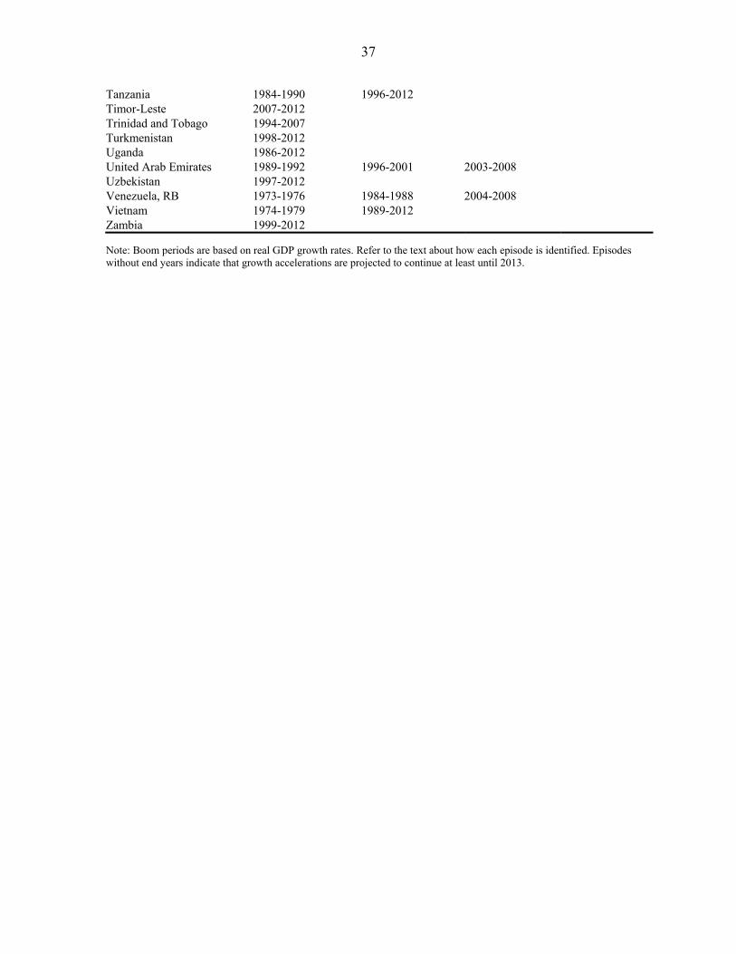
37

Tanzania 1984-1990 1996-2012 Timor-Leste 2007-2012 Trinidad and Tobago 1994-2007 Turkmenistan 1998-2012 Uganda 1986-2012 United Arab Emirates 1989-1992 1996-2001 2003-2008 Uzbekistan 1997-2012 Venezuela, RB 1973-1976 1984-1988 2004-2008 Vietnam 1974-1979 1989-2012 Zambia 1999-2012

Note: Boom periods are based on real GDP growth rates. Refer to the text about how each episode is identified. Episodes without end years indicate that growth accelerations are projected to continue at least until 2013.

38

Figure 1. The number of countries with stabilization funds – by region and establishment year

Note: There are a total of 32 countries, including Ecuador, who has already abolished the fund. If two and more stabilization funds have been created in a country, the establishment year of the first fund is used. Refer to Appendix 2 for the list of stabilization funds and their establishment years. Countries are grouped by area department of the IMF: MCD (Middle East and Central Asia Department), APD (Asia and Pacific Department), WHD (Western Hemisphere Department), AFR (African Department) and EUR (European Department). Source: Author’s compilation.

0

2

4

6

8

10

MCD APD WHD AFR EUR

2000-11

1990-99

1980-89

Pre-1980

Year ofEstablishment

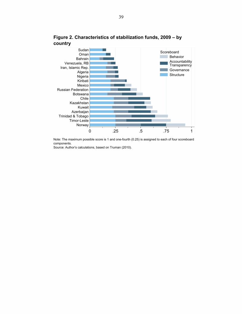
39

Figure 2. Characteristics of stabilization funds, 2009 – by country

Note: The maximum possible score is 1 and one-fourth (0.25) is assigned to each of four scoreboard components. Source: Author’s calculations, based on Truman (2010).

0 .25 .5 .75 1

NorwayTimor-Leste

Trinidad & TobagoAzerbaijan

KuwaitKazakhstan

ChileBotswana

Russian FederationMexicoKiribatiNigeriaAlgeria

Iran, Islamic Rep.Venezuela, RB

BahrainOmanSudan

BehaviorAccountabilityTransparencyGovernanceStructure

Scoreboard

40

Figure 3. Assets of stabilization funds, percentage of GDP, 2009 – by country

Note: The numbers in parentheses next to country names are the asset amounts in billions of US dollars. Source: Author’s calculations, based on Truman (2010), IMF World Economic Outlook and United Nations National Account Main Aggregate Database.

365.0332.1

191.6184.8

114.0111.0110.6

72.651.8

40.029.428.6

16.615.115.110.59.96.53.62.50.90.70.20.2

0 100 200 300 400

Tuvalu (0.1B)Kiribati (0.4B)Kuwait (203B)

Timor-Leste (4.8B)Norway (432B)

Libya (70B)Nauru (0.06B)Bahrain (14B)

Botswana (6B)Algeria (55B)

Azerbaijan (13B)Kazakhstan (33B)

Oman (8B)Russian Federation (185B)

Trinidad & Tobago (2.9B)Chile (18B)

Mauritania (0.3B)Nigeria (11B)

Iran, Islamic Rep. (13B)Turkmenistan (0.5B)

Colombia (2.1B)Mexico (6B)

Venezuela, RB (0.8B)Sudan (0.1B)

41

Figure 4. Trends in the expenditure volatility in countries with and without stabilization funds

A. 6-year period B. 8-year period

Note: The vertical axis shows the discretionary expenditure volatility in logs. The base years of the control group (i.e., countries without stabilization funds—“without funds” group), t, are 1998 and 1999, respectively, in Panels A and B. For countries with stabilization funds (i.e., treatment (“with funds”) group), t is always the year when their first fund was created (with 5-year lagged). The shared area (from t-2 or t-3 to t) shows the expenditure volatility over the period before stabilization funds are established in the treatment group. Source: Author’s calculations, based on IMF World Economic Outlook.

Without funds

With funds

1.8

2

2.2

2.4

2.6

2.8

t-2 t-1 t t+1 t+2 t+3

Without funds

With funds

1.8

2

2.2

2.4

2.6

2.8

t-3 t-2 t-1 t t+1 t+2 t+3 t+4

42

Table 1. Estimation results with discretionary spending volatility (dependent variable: volatility of discretionary government expenditure, in logs)

Note: Data are over the period of 1993–2012 (unbalanced panel). Panel-corrected standard errors are presented in brackets below the corresponding coefficients. *, ** and *** denote statistical significance at the 10 percent, 5 percent and 1 percent levels, respectively.

[1] [2] [3] [4] [5] [6] [7]

Presence of stabilization fund -0.217 -0.224 -0.166 -0.138 -0.299 -0.249 -0.304(dummy variable, t -5) [0.071]*** [0.063]*** [0.072]** [0.059]** [0.078]*** [0.075]*** [0.070]***

Economic structure (t -5)

Government expenditure -0.154 -0.129 -0.009 0.005 -0.094 0.016 0.013(percentage of GDP, in logs) [0.048]*** [0.052]** [0.040] [0.045] [0.048]* [0.040] [0.044]

Population -0.175 -0.157 -0.151 -0.146 -0.169 -0.155 -0.146(in logs) [0.005]*** [0.006]*** [0.007]*** [0.006]*** [0.005]*** [0.006]*** [0.005]***

GDP per capita, PPP -0.121 -0.104 0.023 -0.006 -0.102 0.012 -0.005(constant 2005 international dollars, in logs) [0.016]*** [0.020]*** [0.025] [0.028] [0.019]*** [0.028] [0.029]

Diversification of export products 0.109 0.100 0.065 0.045 0.057 0.037 0.038(Theil index: higher, less diversified) [0.018]*** [0.014]*** [0.012]*** [0.014]*** [0.019]*** [0.017]** [0.016]**

Real sector management (t -5)

Real GDP growth volatility 0.216 0.149 0.185 0.150(5-year moving standard deviation, in logs) [0.016]*** [0.016]*** [0.016]*** [0.017]***

CPI inflation 0.008 0.005 0.009 0.005(percent) [0.003]*** [0.002]** [0.003]*** [0.002]**

Financial market (t -5)

Liquid liabilities -0.353 -0.200 -0.314 -0.202(percentage of GDP, in logs) [0.041]*** [0.044]*** [0.049]*** [0.044]***

Volatility of liquid liabilities 0.148 0.059 0.119 0.055(5-year moving standard deviation, in logs) [0.029]*** [0.031]* [0.032]*** [0.032]*

International financial remoteness 0.339 0.322 0.326 0.318(distance to financial center, km, in logs) [0.028]*** [0.023]*** [0.024]*** [0.022]***

Capital account openness -0.078 -0.055 -0.066 -0.055(index: higher, more openness) [0.012]*** [0.016]*** [0.013]*** [0.016]***

Political institution (t -5)

Political freedom 0.048 0.062 0.042 0.036(index: higher, less freedom) [0.015]*** [0.012]*** [0.019]** [0.017]**

Interaction 0.044 0.035 0.042× Presence of stabilization fund [0.017]*** [0.018]* [0.018]**

Constant 6.026 5.298 2.466 1.997 5.261 2.477 2.084[0.150]*** [0.181]*** [0.374]*** [0.339]*** [0.179]*** [0.373]*** [0.334]***

Number of observations 807 807 807 807 807 807 807Number of countries 62 62 62 62 62 62 62R² 0.20 0.30 0.33 0.38 0.33 0.35 0.38

43

Table 2. Using alternative volatility definitions (dependent variable: volatility of government expenditure and fiscal balance, in logs)

Note: Data are over the period of 1993-2012 (unbalanced panel). In columns 1 to 6, only the growth acceleration (i.e., economic boom) periods are considered. Appendix 5 has the list of boom episodes. Panel-corrected standard errors are presented in brackets below the corresponding coefficients. *, ** and *** denote statistical significance at the 10 percent, 5 percent and 1 percent levels, respectively.

[1] [2] [3] [4] [5] [6] [7] [8]

Presence of stabilization fund -0.054 -0.154 0.006 -0.426 -0.339 -1.132 -0.227 -0.421(dummy variable, t -5) [0.060] [0.100] [0.053] [0.156]*** [0.071]*** [0.164]*** [0.059]*** [0.125]***

Economic structure (t -5)

Government expenditure -0.160 -0.155 -0.099 -0.099 -0.329 -0.359 0.850 0.859(percentage of GDP, in logs) [0.051]*** [0.051]*** [0.071] [0.074] [0.123]*** [0.119]*** [0.081]*** [0.082]***

Population -0.133 -0.132 -0.115 -0.110 -0.291 -0.284 -0.146 -0.146(in logs) [0.012]*** [0.012]*** [0.020]*** [0.021]*** [0.041]*** [0.039]*** [0.014]*** [0.014]***

GDP per capita, PPP -0.102 -0.098 -0.133 -0.105 -0.281 -0.238 0.027 0.029(constant 2005 international dollars, in logs) [0.020]*** [0.023]*** [0.022]*** [0.030]*** [0.038]*** [0.043]*** [0.031] [0.030]

Diversification of export products 0.137 0.132 0.051 0.040 0.238 0.219 0.274 0.265(Theil index: higher, less diversified) [0.020]*** [0.021]*** [0.018]*** [0.021]** [0.027]*** [0.029]*** [0.036]*** [0.035]***

Real sector management (t -5)

Real GDP growth volatility 0.189 0.190 0.159 0.159 0.268 0.275 0.102 0.104(5-year moving standard deviation, in logs) [0.026]*** [0.026]*** [0.034]*** [0.032]*** [0.050]*** [0.048]*** [0.027]*** [0.028]***

CPI inflation 0.003 0.003 0.009 0.009 0.015 0.015 -0.008 -0.008(percent) [0.003] [0.003] [0.003]*** [0.003]*** [0.004]*** [0.004]*** [0.004]** [0.004]**

Financial market (t -5)

Liquid liabilities -0.102 -0.107 -0.016 -0.047 0.006 -0.027 -0.251 -0.253(percentage of GDP, in logs) [0.055]* [0.058]* [0.063] [0.063] [0.106] [0.101] [0.076]*** [0.077]***

Volatility of liquid liabilities 0.099 0.097 0.032 0.029 -0.058 -0.073 0.119 0.114(5-year moving standard deviation, in logs) [0.036]*** [0.035]*** [0.043] [0.041] [0.059] [0.057] [0.043]*** [0.042]***

International financial remoteness 0.073 0.072 -0.173 -0.178 -0.040 -0.057 0.009 0.004(distance to financial center, km, in logs) [0.056] [0.056] [0.061]*** [0.056]*** [0.065] [0.072] [0.060] [0.058]

Capital account openness 0.013 0.013 -0.005 -0.009 0.020 0.015 0.028 0.028(index: higher, more openness) [0.018] [0.017] [0.020] [0.018] [0.028] [0.025] [0.012]** [0.012]**

Political institution (t -5)

Political freedom 0.059 0.050 0.035 -0.003 0.048 -0.020 0.009 -0.005(index: higher, less freedom) [0.014]*** [0.017]*** [0.017]** [0.018] [0.027]* [0.031] [0.020] [0.023]

Interaction 0.024 0.098 0.185 0.049× Presence of stabilization fund [0.022] [0.037]*** [0.036]*** [0.024]**

Constant 4.440 4.460 7.034 7.084 8.592 8.869 -0.217 -0.116[0.542]*** [0.537]*** [0.977]*** [0.924]*** [0.990]*** [1.045]*** [0.926] [0.907]

Number of observations 507 507 473 473 474 474 807 807Number of countries 57 57 52 52 53 53 62 62R² 0.42 0.42 0.22 0.23 0.43 0.45 0.39 0.40

Overall Investment Consumption

Unadjusted: Boom periods onlyCyclically-adjusted

fiscal balance

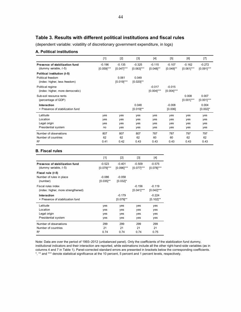
44

Table 3. Results with different political institutions and fiscal rules (dependent variable: volatility of discretionary government expenditure, in logs)

A. Political institutions

B. Fiscal rules

Note: Data are over the period of 1993–2012 (unbalanced panel). Only the coefficients of the stabilization fund dummy, institutional indicators and their interaction are reported, while estimations include all the other right-hand-side variables (as in columns 4 and 7 in Table 1). Panel-corrected standard errors are presented in brackets below the corresponding coefficients. *, ** and *** denote statistical significance at the 10 percent, 5 percent and 1 percent levels, respectively.

[1] [2] [3] [4] [5] [6] [7]

Presence of stabilization fund -0.196 -0.135 -0.325 -0.115 -0.107 -0.162 -0.272(dummy variable, t -5) [0.059]*** [0.047]*** [0.063]*** [0.048]** [0.049]** [0.061]*** [0.091]***

Political institution (t -5)

Political freedom 0.061 0.049(index: higher, less freedom) [0.019]*** [0.020]**

Political regime -0.017 -0.015(index: higher, more democratic) [0.004]*** [0.004]***

Sub-soil resource rents 0.008 0.007(percentage of GDP) [0.001]*** [0.001]***

Interaction 0.048 -0.008 0.004× Presence of stabilization fund [0.019]** [0.006] [0.002]*

Latitude yes yes yes yes yes yes yesLocation yes yes yes yes yes yes yesLegal origin yes yes yes yes yes yes yesPresidential system no yes yes yes yes yes yes

Number of observations 807 807 807 787 787 797 797Number of countries 62 62 62 60 60 62 62R² 0.41 0.42 0.43 0.43 0.43 0.43 0.43

[1] [2] [3] [4]

Presence of stabilization fund -0.523 -0.401 -0.509 -0.575(dummy variable, t -5) [0.079]*** [0.096]*** [0.077]*** [0.078]***

Fiscal rule (t -5)

Number of rules in place -0.086 -0.058(number) [0.035]** [0.032]*

Fiscal rules index -0.156 -0.119(index: higher, more strengthened) [0.041]*** [0.042]***

Interaction -0.179 -0.224× Presence of stabilization fund [0.079]** [0.102]**

Latitude yes yes yes yesLocation yes yes yes yesLegal origin yes yes yes yesPresidential system yes yes yes yes

Number of observations 299 299 299 299Number of countries 21 21 21 21R² 0.74 0.74 0.74 0.75

45

Table 4. Countries with stabilization funds only (dependent variable: volatility of discretionary government expenditure, in logs)

Note: Data are over the period of 1993-2012 (unbalanced panel). Only 32 countries that have ever established stabilization funds are used. Panel-corrected standard errors are presented in brackets below the corresponding coefficients. *, ** and *** denote statistical significance at the 10 percent, 5 percent and 1 percent levels, respectively.

[1] [2] [3] [4] [5] [6] [7]

Presence of stabilization fund -0.358 -0.352 -0.372 -0.251 -0.536 -0.515 -0.505(dummy variable, t -5) [0.047]*** [0.044]*** [0.069]*** [0.060]*** [0.090]*** [0.109]*** [0.100]***

Economic structure (t -5)

Government expenditure -0.054 -0.036 -0.013 0.000 0.025 0.045 -0.016(percentage of GDP, in logs) [0.041] [0.040] [0.062] [0.060] [0.040] [0.058] [0.059]

Population -0.131 -0.127 -0.106 -0.116 -0.131 -0.103 -0.122(in logs) [0.012]*** [0.011]*** [0.015]*** [0.012]*** [0.011]*** [0.012]*** [0.011]***

GDP per capita, PPP -0.176 -0.155 -0.205 -0.250 -0.154 -0.223 -0.250(constant 2005 international dollars, in logs) [0.020]*** [0.021]*** [0.029]*** [0.024]*** [0.021]*** [0.030]*** [0.028]***

Diversification of export products 0.163 0.151 0.155 0.120 0.088 0.099 0.104(Theil index: higher, less diversified) [0.010]*** [0.011]*** [0.012]*** [0.016]*** [0.016]*** [0.016]*** [0.018]***

Real sector management (t -5)

Real GDP growth volatility 0.109 0.073 0.083 0.083(5-year moving standard deviation, in logs) [0.026]*** [0.026]*** [0.026]*** [0.026]***

CPI inflation 0.002 0.010 0.004 0.009(percent) [0.003] [0.003]*** [0.003]* [0.003]***

Financial market (t -5)

Liquid liabilities 0.004 0.176 0.053 0.181(percentage of GDP, in logs) [0.056] [0.060]*** [0.059] [0.059]***

Volatility of liquid liabilities 0.147 0.065 0.108 0.055(5-year moving standard deviation, in logs) [0.048]*** [0.047] [0.047]** [0.044]

International financial remoteness 0.202 0.116 0.171 0.118(distance to financial center, km, in logs) [0.068]*** [0.060]* [0.060]*** [0.057]**

Capital account openness 0.038 0.067 0.054 0.067(index: higher, more openness) [0.020]* [0.016]*** [0.016]*** [0.016]***

Political institution (t -5)

Political freedom 0.077 0.030 0.044 0.044(index: higher, less freedom) [0.013]*** [0.018]* [0.025]* [0.022]**

Interaction 0.069 0.055 0.063× Presence of stabilization fund [0.023]*** [0.023]** [0.024]***

Constant 5.351 4.973 3.345 3.647 4.961 3.426 3.981[0.356]*** [0.338]*** [0.734]*** [0.623]*** [0.267]*** [0.689]*** [0.630]***

Number of observations 395 395 395 395 395 395 395Number of countries 29 29 29 29 29 29 29R² 0.31 0.33 0.36 0.42 0.37 0.40 0.43

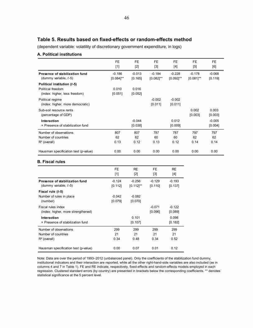
46

Table 5. Results based on fixed-effects or random-effects method (dependent variable: volatility of discretionary government expenditure, in logs)

A. Political institutions

B. Fiscal rules

Note: Data are over the period of 1993–2012 (unbalanced panel). Only the coefficients of the stabilization fund dummy, institutional indicators and their interaction are reported, while all the other right-hand-side variables are also included (as in columns 4 and 7 in Table 1). FE and RE indicate, respectively, fixed-effects and random-effects models employed in each regression. Clustered standard errors (by country) are presented in brackets below the corresponding coefficients. ** denotes statistical significance at the 5 percent level.

FE FE FE FE FE FE[1] [2] [3] [4] [5] [6]

Presence of stabilization fund -0.186 -0.013 -0.184 -0.228 -0.178 -0.068(dummy variable, t -5) [0.084]** [0.165] [0.082]** [0.092]** [0.081]** [0.119]

Political institution (t -5)

Political freedom 0.010 0.016(index: higher, less freedom) [0.051] [0.052]

Political regime -0.002 -0.002(index: higher, more democratic) [0.011] [0.011]

Sub-soil resource rents 0.002 0.003(percentage of GDP) [0.003] [0.003]

Interaction -0.044 0.012 -0.005× Presence of stabilization fund [0.038] [0.009] [0.004]

Number of observations 807 807 787 787 797 797Number of countries 62 62 60 60 62 62R² (overall) 0.13 0.12 0.13 0.12 0.14 0.14

Hausman specification test (p-value) 0.00 0.00 0.00 0.00 0.00 0.00

FE RE FE RE[1] [2] [3] [4]

Presence of stabilization fund -0.124 -0.256 -0.129 -0.193(dummy variable, t -5) [0.112] [0.112]** [0.110] [0.137]

Fiscal rule (t -5)

Number of rules in place -0.042 -0.082(number) [0.079] [0.070]

Fiscal rules index -0.071 -0.122(index: higher, more strengthened) [0.096] [0.089]

Interaction 0.101 0.098× Presence of stabilization fund [0.107] [0.182]

Number of observations 299 299 299 299Number of countries 21 21 21 21R² (overall) 0.34 0.48 0.34 0.52

Hausman specification test (p-value) 0.00 0.07 0.01 0.12

47

Table 6. Difference-in-differences estimation with panel data (dependent variable: volatility of discretionary government expenditure, in logs)

Note: Only the coefficient of the stabilization fund dummy is presented in the left part of the table. While the base year of the control group is 1998, 1999 and 2000, the base year of the treatment group is always the same and decided by when the first stabilization fund was established. The right part of the table shows p-values of the test which null hypothesis is that the two groups have the same trends in the expenditure volatility in the “pre” period. *, ** and *** denote statistical significance at the 10 percent, 5 percent and 1 percent levels, respectively.

2 years 3 years 4 years

Presence of stabilization fund

Estimation based on: p-value

Political freedom(Base year of control group)

t = 1998 -0.152 [0.088]* -0.219 [0.093]** -0.165 [0.101] 0.318 0.277 0.477t = 1999 -0.234 [0.105]** -0.220 [0.113]* -0.202 [0.097]** 0.983 0.713 0.508t = 2000 -0.091 [0.138] -0.170 [0.127] -0.149 [0.124] 0.825 0.491 0.688

Political regime(Base year of control group)

t = 1998 -0.138 [0.091] -0.214 [0.093]** -0.153 [0.099] 0.180 0.352 0.390t = 1999 -0.230 [0.098]** -0.210 [0.104]** -0.187 [0.092]* 0.989 0.709 0.240t = 2000 -0.095 [0.128] -0.175 [0.120] -0.143 [0.118] 0.824 0.449 0.700

Sub-soil resource rents(Base year of control group)

t = 1998 -0.183 [0.091]* -0.269 [0.095]*** -0.206 [0.099]** 0.163 0.519 0.443t = 1999 -0.245 [0.107]** -0.244 [0.111]** -0.234 [0.097]** 0.412 0.578 0.718t = 2000 -0.101 [0.134] -0.206 [0.128] -0.175 [0.122] 0.722 0.552 0.542

2 years 3 years 4 years

Year dummies are same in 'pre' period

Years covered in 'pre' and 'post' periods

48

Table 7. Difference-in-differences estimation with two-period data (dependent variable: volatility of discretionary government expenditure, in logs)

Note: The base year, t, of the control group is 1998, 1999 and 2000 in Panels A, B and C, respectively. For the treatment group, the base year is decided by when the first stabilization fund was established. *, ** and *** denote statistical significance at the 10 percent, 5 percent and 1 percent levels, respectively.

Pre Post Pre Post Pre Post

Period average:

Base year of control group = tA. t=1998

With funds -2.752 -2.858 -1.873 -1.994 -1.790 -1.853[4.743] [4.753] [3.548] [3.549] [2.714] [2.703]

Without funds -3.052 -2.762 -2.175 -1.921 -2.088 -1.861[4.817] [4.747] [3.562] [3.533] [2.702] [2.659]

Difference 0.300 -0.096 0.302 -0.073 0.298 0.008[0.235] [0.245] [0.233] [0.240] [0.221] [0.191]

Difference-in-difference -0.396 -0.375 -0.290[0.143]*** [0.130]*** [0.145]*

B. t=1999

With funds -3.078 -3.177 -2.894 -3.007 -2.001 -2.055[3.632] [3.634] [2.988] [2.985] [2.666] [2.655]

Without funds -3.315 -3.104 -3.197 -3.015 -2.273 -2.103[3.684] [3.626] [3.009] [2.950] [2.666] [2.630]

Difference 0.237 -0.073 0.302 0.008 0.271 0.048[0.261] [0.223] [0.233] [0.190] [0.224] [0.167]

Difference-in-difference -0.311 -0.294 -0.224[0.137]** [0.154]* [0.140]

C. t=2000

With funds -3.530 -3.621 -2.506 -2.603 -1.387 -1.433[2.420] [2.417] [2.503] [2.503] [2.120] [2.110]

Without funds -3.650 -3.674 -2.699 -2.689 -1.518 -1.490[2.399] [2.372] [2.481] [2.478] [2.107] [2.114]

Difference 0.121 0.053 0.192 0.085 0.130 0.058[0.238] [0.190] [0.225] [0.177] [0.189] [0.140]

Difference-in-difference -0.068 -0.107 -0.073[0.160] [0.156] [0.152]

2 years 3 years 4 years

Establishment of stabilization fund