Effectiveness of Stabilization Funds in

Managing Volatility in Oil-Rich Countries

Gunes A. Asik ∗

TOBB Economics and Technology University

July 26, 2017

Abstract

This paper explores whether sovereign wealth or stabilization

funds created by governments in oil rich countries are effective in

reducing volatility and ensuring a counter-cyclical or acyclical fiscal

policy in line with the findings of optimal fiscal policy literature.

Existing literature on the effectiveness of stabilization funds suffers

from endogeneity problems, namely i) the endogeneity between GDP

and government expenditures and ii) the endogeneity of the decision

to establish stabilization funds. In this paper, I contribute to the

literature by addressing both of these problems by using series of

Two Stage Least Square Estimations and find positive evidence in

favor of stabilization funds in reducing volatility and procyclicality

of fiscal policy. The findings are relevant for the wider discussion

of the procyclicality in developing countries, as one third of the

countries which are documented to improve fiscal policy cyclicality

seem to be the ones that are resource rich and have a stabilization

fund in place.

Keywords: Oil Stabilization Funds, Fiscal Policy, Volatility, Business Cycles

∗Electronic address: gasik@etu.edu.tr I would like to thank Chris Pissarides, Mum-

taz Hussain, Steve Pischke, Francesco Caselli, Silvana Tenreyro, Ethan Izetzki, Andres

Zahler and other seminar particiants at London School of Economics and TOBB Eco-

nomics and Technology University for useful comments and guidance.

1

1 Introduction:

Fluctuating natural resource and commodity prices typically create

boom and bust cycles in the natural resource rich economies and lead to

an erratic growth performance under the absence of prudent fiscal policies.

Stabilization Funds are special purpose investment funds or arrangements

created by governments for macroeconomic management purposes. They

hold and manage assets that are proceeds of natural resource/commodity

export revenues, balance of payments surpluses, privatization or foreign

currency operations. These special purpose funds include sovereign wealth

funds, fiscal stabilization funds, savings funds, reserve investment corpo-

rations, development funds, and pension reserve funds without liabilities.

According to the data by the Sovereign Wealth Instutite, the total asset size

of the sovereign wealth funds worldwide as of December 2015 was about

USD 7,193 billion, USD 4,048 billion of which is oil and gas related.1 The

aim of this paper is to investigate the effectiveness of stabilization and

savings funds which are established to accumulate oil and gas revenues to

finance certain investments and expenditures or smooth the fiscal revenues

in the face of highly volatile international prices. By ‘effectiveness’ I mainly

refer to the degree of fiscal countercyclicality or acyclicality given the ob-

jective of smoothing fiscal expenditures and revenues through creating a

‘tool’ for saving.

The question of whether the stabilization funds are effective is an im-

portant one because in a way, it relates to the broader discussion of whether

the fiscal policy in developing countries have become less procyclical. A

study by Frankel, Vegh and Vuletin (2012) show that there is a group

of countries that have graduated from fiscal procyclicality, meaning that

the fiscal policy have become countercyclical. One third of the countries

in the ‘graduation list’ however comprises countries that are resource rich

and have a stabilization fund in place.2 The study by Frankel et al (2012)

argue that the main determinant of whether a country graduates from pro-

1http://www.swfinstitute.org/sovereign-wealth-fund-rankings/2Graduated countries in the list are Algeria, Bahrain, Chile, Libya, Nigeria, Norway,

Oman, Saudi Arabia, United Arab Emirates, Bolvia, Botswana, Brazil, Costa Rica, Coted’Ivoire, El Salvador, Germany, Hong Kong, Indonesia, Malaysia, Morocco, Paraguay,Phillipines, Syrian Arab Republic, Turkey, Uganda and Zambia where the first nine havea stabilization fund in place. See Frankel et al. (2013, Fig.4)

2

cyclicality is the institutional quality. Using instruments for potentially

endogenous variables, the study concludes that there is a strong causal

link from better institutions to less procyclical policies. As I show below,

some part of the graduation is actually due to creating a mechanism to

further tie the hands of the governments in oil rich countries, even after

controlling for institutional quality differences.

From a theoretical point of view, there would be no reason for any re-

source rich country to establish stabilization or savings funds if there were

perfect insurance markets. However, the experience shows that the num-

ber of such funds started to increase dramatically especially towards the

end of 1990s and most of the oil producer countries seem to have relied

upon funds, rather than relying on insurance markets. Moreover, there is

a vast literature showing that the external capital inflows are highly pro-

cyclical, making borrowing more difficult during times of negative shocks.

Therefore during the times of high capital inflows, the business cycles are

further exacerbated through expansionary fiscal policies. This phenomenon

is described as ‘when it rains, it pours’ by Kamisnky, Reinhart and Vegh

(2004). Ilzetski (2011) show that a political economy model with resdis-

tributive government policies and borrowing constraints can explain pro-

cyclical fiscal policies only during economic downturns, and introducing

political polarization to the model significantly improves the ability to ex-

plain differences in fiscal policy accross countries.3

In this paper, I take an agnostic view on whether the international

capital markets are imperfect as well as on why any country would pursue

a procyclical fiscal policy that aggrevates the business cycles. In line with

the theoretical prescriptions, I assume that the optimal fiscal policy is either

countercyclical (in a Keynesian setting) or acyclical following Barro’s tax

smoothing result (in the Neoclassical setting).4 I take the view that it

might be due to the fact that stabilization funds provide a mechanism for

self-insurance to accumulate resources and smooth expenditures, and this

might be the reason why resource rich countries which are vulnerable to

external conditions have started to rely on them one after another. In

3For a discussion of causes of procyclical fiscal policies in developing countries, seeIlzetski (2011) and Jaimovich and Panizza (2007, p.4-6)

4For a short discussion, see Ilzetzki and Vegh (2008, p.4-6)

3

this paper, I ask the question whether such funds indeed help countries

to achive better fiscal policy outcomes that are closer to the optimal fiscal

policy framework prescribed by the theory.5

I use a sample of 29 oil-rich countries, namely; Algeria, Angola, Azer-

baijan, Bahrain, Bolivia, Brazil, Cameroon, Chad, Republic of Congo,

Ecuador, Gabon, Indonesia, Islamic Republic of Iran, Kazakhstan, Kuwait,

Libya, Mexico, Nigeria, Norway, Oman, Qatar, Russian Federation, Saudi

Arabia, Sudan, Trinidad and Tobago, United Arab Emirates, Venezuela,

Vietnam and Yemen for the period between 1980-2012. I find that the fiscal

policy is indeed highly procyclical in oil-rich countries without funds and

they are mildly procyclical or acyclical in countries with stabilization or

savings funds. Moreover, I find evidence that the volatility of major macro

variables of interest such as the volatility of real household consumption,

real government expenditures and government consumption as well as gross

fixed capital investments are lower in those countries with such funds. Run-

ning seperate estimations only for countries with funds for the 1980-2012

period show that the procyclicality result becomes statistically insignifi-

cant (before and after), supporting the view that countries that establish

such saving mechanisms might be more prudent to start with as opposed to

countries without funds. If so, the results are supportive of the findings by

Frankel et al (2012) who suggest that the ‘graduating class’ are the more

prudent ones with better institutions, although I do not find a statistically

significant association between fiscal performance and institutional quality

in my sample of oil-rich countries.6.

This paper is among the few to investigate whether stabilization or sav-

ings funds deliver more desirable outcomes. The existing results in the lit-

erature with respect to the experience with funds are mixed though. A case

study by Fasano (2000) suggests that in some countries like Kuwait, Nor-

way and State of Alaska, savings funds have contributed to enhancing the

effectiveness of fiscal policy by making the budget expenditures less driven

5By ‘outcomes’, I mean ‘directly controllable fiscal policy realizations’ such as gov-ernment expenditures rather than budget balance which is not entirely controllable bythe government due to revenue collection aspect. I will elaborate this point in Section2.

6Insignificance of the coefficients for institutional quality measures could be due tothe fact that there is not much institutional quality variation across countries, with theexception of Norway

4

by revenue availability, whereas in other countries the experience has been

less successful because of frequent changes to fund rules and the deviation

from its intended purposes.7 Fasano (2000) suggests that such funds have

been more successful in countries with a strong commitment to fiscal dis-

cipline and sound macroeconomic management and the experience shows

that funds should not be considered as a substitute for sound fiscal manage-

ment. Another study by Husain, Tazhibayeva and Ter-Martirosyan (2008)

suggests that the economic output in oil-exporting countries is strongly af-

fected by oil prices and investigate whether the world oil price changes have

an independent influence on economic activity or whether the channel is

through the impact of procyclical fiscal policies on the economic activity.8

Findings support the view that procyclical fiscal policies in oil exporting

countries is the main mechanism by which oil price shocks are transmitted

to the non-oil economy.

The study by Shabsigh and Ilahi (2007) uses a panel data set consist-

ing of 15 oil-rich countries with and without stabilization funds for the

period 1973-2003. The study asks whether having a stabilization fund is

associated with having lower volatility in an oil-rich economy. The study

finds evidence of a robust negative relationship between the existence of

an oil fund and inflation, volatility of broad money, real exchange rate

and prices in oil-exporting countries. Main challenges in establishing a

robust empirical relation between the existence of stabilization funds and

better fiscal outcomes are unobserved heterogeneity, endogeneity and the

difficulty of distinguishing the impact of the introduction of funds which

overlap with the beginning of an oil-boom. The study partially addresses

these challenges by using fixed effects estimator to remove the impact of

time-invariant variables. The econometric specification however, cannot

capture the role of time-variant factors and endogeneity of oil funds.

Ossowski, Villafuerte, Medas and Thomas (2008) also use panel data

consisting of 32 oil-rich countries with and without a stabilization fund

7The study covers the experience of Norway, Chile, Venezuela, State of Alaska,Kuwait and Oman.

8The study estimates impulse responses to oil shocks based on panel VARs of oilprices, fiscal stance and output. The countries analyzed include Iran, Norway, Yemen,Algeria, U.A.E. Nigeria, Saudi Arabia, Libya, Oman and Kuwait.

5

and/or a fiscal rule in place between 1992 and 2005.9 The empirical ques-

tion is whether having a stabilization fund and/or a fiscal policy rule leads

to i) lower change in non-oil primary primary balance as a percent of non-

oil GDP , ii) lower change in real government expenditures, iii) lower ratio

of the change in expenditures to the change in oil revenues in an oil-rich

country. Prefered specification is fixed effects estimator again to address

the problem of time-invariant factors affecting the outcome variables. In

addition, Arellano and Bond (1991) dynamic GMM estimator is introduced

to address the possible endogeneity problem, i.e. a fiscal rule/fund could

be introduced because of the existence of imprudent fiscal outcomes. The

study controls for the institutional factors using International Country Risk

Guide data on democratic accountability, bureaucratic quality, government

stability and law and order. Contrary to the findings of Shabsigh and Ilahi

(2007), Ossowski, Villafuerte, Medas and Thomas (2008) cannot find evi-

dence of a positive impact on fiscal outcomes.

A survey by Devlin and Titman (2004) suggests that the extent to

which savings and stabilization funds can smooth out investment and rev-

enues depends on the random process generating the commodity/natural

resource prices. When price changes are mean-reverting, the present value

of the future revenues are not strongly affected by the spot prices therefore

will not diminish the efficiency of funding for expenditures, whereas with a

random walk process/permanent price changes, present value of future oil

revenues will be large, and so will be the optimal level of investment. In

that case, financial instruments rather than stabilization or savings funds

will be more effective to deal with the fluctuations caused by price changes.

When price changes are permanent, stabilization funds end up constantly

accumulating or depleting assets which do not help reduce the volatility in

the economy. However, this is a channel which has not been investigated in

by the empirical literature on the effectiveness of stabilization funds. The

evidence on whether the oil prices are mean-reverting though is mixed.

Pindyck (1999) and Barnett and Vivanco (2003) show evidence on mean-

reversion whereas Cashin, Liang and McDermott (2000) and Engel and

Valdes (2000) find evidence of persistence. Bartsch (2006) makes the point

9Their analysis covers the oil-producing countries where fiscal revenue accounted forat least 20 percent of total fiscal revenue in 2004.

6

that the international oil prices show very weak mean reversion and studies

the implications and fiscal policy design for Nigeria. The study suggests

that Nigeria as an oil producing country should base its estimates of ex-

pected revenues and expenditures on the moving averages of past oil prices

because the long-term average oil price is of little use for policy making due

to weak mean reversion. Using moving averages of three to five years would

lead to smallest forecast error, and reduce the risk of building large and

persistent surpluses or deficits given the slow mean reversion of oil prices.

I believe that the existing studies, albeit enlightening do not adequately

answer the question whether such funds are effective and should be prescibed

for any resource rich country. The existing analyses do not differentiate be-

tween long-run trends or cyclical fluctuations, do not investigate the out-

comes in line with the optimal fiscal policy prescriptions, do not carefully

handle the problem of endogeneity of the following three; i) GDP, ii) the

decision to establish a fund, and iii) the institutions. And finally, existing

studies do not properly assess the volatility although the economic theory

suggests that there are welfare costs of business cycle fluctuations. More-

over, I believe that those studies focus on the wrong fiscal policy outcomes

which are usually not directly controllable by fiscal agencies. In this pa-

per, I aim to contribute to the existing literature by addressing all these

concerns, especially the endogeneity issue.

In order to address the endogeneity between the GDP and government

expenditures, I use the external shock instrument for the GDP, as proposed

by Jaimovich and Panizza (2007). As for the endogeneity of the ‘decision

to establish a fund’, I use urbanization, and the lags of both the average

years of schooling and percent of population with tertiary education in or-

der to proxy for awareness for ‘better management of people’s resources’.

As it will be explained in more detail in Section 3, as an extention, I in-

teract the urbanization with the number of other oil-rich countries and

use this new variable along the freedom of press rating as an alternative

proxy for information for the use of resources. And finally, in order to ad-

dress the potential endogeneity of the institutions, I use the lags of average

ICRG ratings of the neighouring countries for each of the oil-rich country in

question. Table 4 summarizes each sets of instruments for the potentially

endogenous variables.

7

The paper is organized as follows: Section 2 discusses the empirical

strategy and the data. Section 3 describes the results of the empirical

analysis where I; i) investigate the cyclical properties under existence of

oil funds using OLS and Two Stage Least Squares Methods, ii) explore

the decision to establish a stabilization fund using several instruments,

iii) instrument institutions which might potentially be endogenous, iv) in-

vestigate the short term growth and volatility of real general government

expenditures, general government final consumption, household final con-

sumption, and gross fixed capital formation as the variables of interest.

Section 4 concludes.

2 Empirical Specification and Data

The experience with stabilization funds is relatively new as most of the

funds were established by the end of 1990s and after year 2000. As Figure

1 shows, there were only 5 countries with oil stabilization funds as of 1994,

whereas after that date, 16 more oil-rich countries adopted some sort of a

fund arrangement.

Figure 1: Number of Countries with Oil Stabilization, Savings or SovereignFunds

The major problem with measuring fiscal policy performance by using

any definitions of the budget balance is that such outcomes are beyond the

full control of the policy makers and can lead to misleading conclusions,

as most studies outlined in the introduction section suffered from. Tax

8

revenues are highly cyclical, and therefore even if government engages in a

completely neutral policy of smooth fiscal expenditures, using the budget

balance as the dependent variable would tell us that the fiscal policy is

countercyclical, being in surplus in good times and in deficit in bad times.

This point has been raised by Kamisky, Reinhart, Vegh (2004), Jaimovich

and Panizza (2007) and Ilzetzki and Vegh (2008) and Vegh and Vuletin

(2013).10

In this paper, I follow the critique above and use general government

expenditures (in real and detrended log terms) as opposed to budget bal-

ance to measure fiscal policy. In other words, I focus directly on the degree

of procyclicality and volatility of expenditures when evaluating the perfor-

mance under stabilization funds. As compared to the previous studies, I

am also able to cover more recent data, namely the period between 1980

and 2012 for a sample of 29 oil-rich countries, namely; Algeria, Angola,

Azerbaijan, Bahrain, Bolivia, Brazil, Cameroon, Chad, Republic of Congo,

Ecuador, Gabon, Indonesia, Islamic Republic of Iran, Kazakhstan, Kuwait,

Libya, Mexico, Nigeria, Norway, Oman, Qatar, Russian Federation, Saudi

Arabia, Sudan, Trinidad and Tobago, United Arab Emirates, Venezuela,

Vietnam and Yemen.11 Table 1 provides the list of countries and Table 2,

the various oil-dependency measures.

Experience shows that in oil rich countries government expenditures

track oil revenues very closely which leads to an erratic fiscal performance

and exacerbate the boom and bust cycles due to changing oil prices in the

economy. The main rationale for establishing a stabilization fund should

be to break this link, and maintain a smoother fiscal policy through sav-

ings in a fund. To a degree, it is perhaps unavoidable that the existence of

the stabilization funds may be weakly associated with lower growth of real

government expenditures because many of the oil-rich countries are on a de-

velopment trajectory with massive infrastructure needs. According to the

World Economic Outlook data of IMF, for instance, the average nominal

10Vegh and Vulent (2013) documents tax-policy procyclicality in developing countriesand acyclicality in developed countries.

11Unfortunately, the panel is unbalanced due to missing data for various countriesand due to the fact that some countries only recently gained independence such asAzerbaijan, Kazakhstan. The specifications with institutinal data (ICRG) cover theperiod 1984-2012)

9

GDP per capita between 2005-2008 was $11,742 for my sample.12. Ex-

cluding high per-capita income countries as United Arab Emirates, Qatar,

Kuwait and Bahrain, the average in the sample drops to $5,452. The

ratio of gross-fixed capital investments to GDP was 23.5% between 1990-

2008. Therefore, the objective of the fiscal policy in a developing country

might not be achiving a lower expenditure growth profile, but instead a

less volatile one where fiscal expenditures do not track revenues closely.

While optimal fiscal policy in Keynesian economics prescibes a counter-

cyclical policy and the Neoclassical point of view prescibes a neutral one

with tax and expenditure smoothing, there is a growing literature showing

that fiscal policy is actually mostly procyclical in many of the developing

countries. In this paper, I also document evidence for procyclicality for

oil-rich countries but investigate whether those oil-rich countries with a

stabilization fund has ‘less procyclical’ fiscal policy- which should be the

objective of establishing the fund in the first place.

The main data source used in this paper is International Monetary

Fund’s (IMF) World Economic Outlook (WEO) and Country Desk Data.

I use annual general government expenditures, however very occasionaly,

I rely on central government expenditures when the data is not available

for general government. The same applies for total general government

revenues, and government oil revenues. Data is reported in nominal terms,

and I deflate it using the CPI index from the same database for each coun-

try. I extract the oil price data from IMF’s WEO as well. The variables in

my regressions are in logs and are detrended by using the Hodrick Prescott

Filter (except for the ratio of oil revenues to total revenues, oil prices and

institutional variables). Using the Augmented Dickey Fuller and Im, Pe-

saran and Shin tests, I am able to reject the null hypothesis of unit root

for the series i) detrended real government expenditures, ii) detrendeded

real government revenues and iii) detrended real GDP with 99% confi-

dence level. In order to capture institutional variables, I use International

Country Risk Guide (ICRG) data which provides political risk ratings on

democratic accountability, bureaucratic quality, law and order, government

stability and corruption for 140 countries since 1984. However, my results

12Excluding Algeria, Ecuador, Iran, Kazakshtan and Saudi Arabia due to non-existence of compatible data.

10

are robust to inclusion of any institutional variable, and in fact, suprisingly

most variables turn out not to have explanatory power on detrended real

government expenditures. The data on household final consumption, gen-

eral government consumption and gross fixed capital formation data are

from WDI. All educational attainment variables are by Barro-Lee (2013)

and are linearly interpolated.

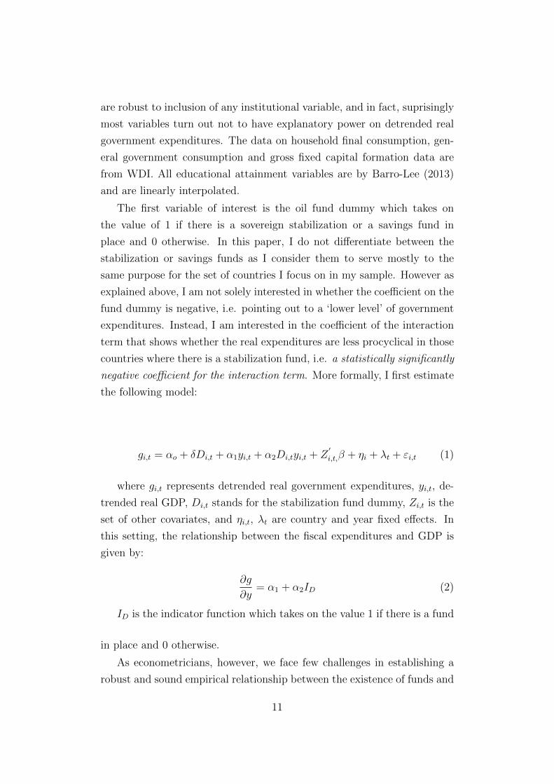
The first variable of interest is the oil fund dummy which takes on

the value of 1 if there is a sovereign stabilization or a savings fund in

place and 0 otherwise. In this paper, I do not differentiate between the

stabilization or savings funds as I consider them to serve mostly to the

same purpose for the set of countries I focus on in my sample. However as

explained above, I am not solely interested in whether the coefficient on the

fund dummy is negative, i.e. pointing out to a ‘lower level’ of government

expenditures. Instead, I am interested in the coefficient of the interaction

term that shows whether the real expenditures are less procyclical in those

countries where there is a stabilization fund, i.e. a statistically significantly

negative coefficient for the interaction term. More formally, I first estimate

the following model:

gi,t = αo + δDi,t + α1yi,t + α2Di,tyi,t + Z′

i,t,β + ηi + λt + εi,t (1)

where gi,t represents detrended real government expenditures, yi,t, de-

trended real GDP, Di,t stands for the stabilization fund dummy, Zi,t is the

set of other covariates, and ηi,t, λt are country and year fixed effects. In

this setting, the relationship between the fiscal expenditures and GDP is

given by:

∂g

∂y= α1 + α2ID (2)

ID is the indicator function which takes on the value 1 if there is a fund

in place and 0 otherwise.

As econometricians, however, we face few challenges in establishing a

robust and sound empirical relationship between the existence of funds and

11

stability of fiscal policy. As I will explain in more detail in the next sec-

tion, the endogeneity of GDP and potential reverse causality is a major

concern which requires careful instrumental variables methods. Another

important challenge is that the decision to adopt a stabilization fund is

not truly exogenous, and countries that run high non-oil deficits might be

more tempted to establish stabilization funds as a self-disciplining mecha-

nism (Ossowski, Villafuerte, Medas and Thomas; 2008, p.32). In that case,

introduction of a fund would seem to be positively associated with higher

fiscal expenditures. Another view suggests that countries that set up sta-

bilization funds maybe more prudent to start with, therefore it would be

inappropriate to attribute their good performance to the funds (Shabsigh

and Ilahi;2007, p.4). In that case, a better fiscal outcome would be asso-

ciated with the unobserved time invariant factors and not necessarily with

the existence of a fund. Under all cases, OLS would yield biased estimates.

While I handle the problem of unobserved time-invariant and time-variant

factors through adopting the fixed effects estimator, random effects estima-

tors and Arellano Bond estimators, admittedly it is a challange to find good

instruments which are highly correlated with introduction of fund dummy

but not directly correlated with fiscal expenditures. To handle the problem

of the endogeneity of ‘introducing a stabilization fund’, I rely on two pos-

sible instruments in Section 3.3 and I find that my results remain robust.

The final challenge I face is that the introduction of an stabilization fund

may coincide with the start of a boom in some countries. In that case oil

expenditures might go up tracking high oil revenues and this would again

appear as if the oil fund is associated with higher expenditure growth. I

handle this problem (at least to a degree) by controlling for the ratio of oil

revenues to total government revenues, which measures the governments’

dependence on oil revenues.

I start by running several sets of estimations in Section 3. In the first

set, I focus on the degree of procyclicality and run OLS estimators, ignoring

the potential endogeneity problem. In the second set, I handle the endo-

geneity problem by using instrumental variables for GDP. In the third set of

estimations, I address the other potential endogeneity problems, which are

namely the decision to establish a fund again and institutions. In Section

3.4 I turn to the question of volatility differences. I measure volatility in

12

terms of moving standard deviations. In all my regressions in Section 3, I

control for the oil dependency (which I measure as the ratio of oil revenues

to total revenues), oil price change and institutional quality measures.

3 Results

3.1 Procyclicality of Fiscal Policy

In this section, I first test the degree of procyclicality for oil rich coun-

tries by usual OLS methods and then use the 2SLS approach as in Jaimovich

and Panizza (2007).13 For each specification, I run two sets of estimations,

one for the whole sample of oil-rich countries, and another for only the

countries with stabilization funds, excluding those which do not have a

fund. The rationale is to see whether the procyclicality results differ when

we focus only on the countries with funds. In all my regressions, I use

detrended (log) real government expenditures as the dependent variable

and detrended (log) real GDP, oil dummy, oil price (log) and share of oil

revenues in total government revenue as independent variables. The latter

variable is used to control for the degree of oil-dependency in the economy.

I also include WDI’s natural resource rents as a percent of GDP as another

control for oil dependency.14 In testing the degree of procyclicality across

countries with and without stabilization funds, I am interested in the sign

and significance of the following coefficients in equation (1);

∂g

∂y= a1 for those countries without/before stabilization funds (3)

∂g

∂y= a1 + a2 for those countries with/after stabilization funds (4)

13In all 2SLS estimations, I also instrument for the interaction term along with theGDP to avoid the “forbidden regression” problem.

14WDI reports total natural resource rents as the difference between the price of acommodity and the average cost of producing it whereby the unit rents are multipliedwith physical quantities.

13

Table 3 shows first set of results. Using the Fixed Effects, Random

Effects and Arellano Bond estimators, I find in the first panel of Table 3

that fiscal policy in a sample of 29 oil rich countries are on average highly

procyclical. The coefficient is around 0.65-0.73 and highly significant in all

specifications using the pooled sample. The results, however also show that

the coefficients of interaction terms are negative and highly statistically sig-

nificant, indicating that the government expenditures are associated signif-

icantly less with GDP, i.e. the fiscal policy is acyclical or mildly procyclical

in those countries where/after there is a stabilization fund for the whole

sample. The coefficient on the stabilization fund dummy is not statistically

significant, indicating that there is no difference on the level of government

expenditures as deviations from the trend across two groups of countries.

Suprisingly, the institutional quality measures are not significant, except for

socioeconomic conditions. The institutional quality measures in the ICRG

dataset are constructed such that higher points indicate better outcomes

and therefore lower risk.15 Hence, the sign of the socioeconomic condi-

tions is indicating that a higher rating of social conditions (therefore lower

social risk) is negatively associated with cyclical fiscal expenditures. The

insignificance of other institutional quality measures especially the corrup-

tion rating could be due to the fact that in our sample most countries have

similar ratings without significant cross country and time variation except

for Norway whereas there is enough variability in socioeconomic conditions

among the rich income per capita and poor income per capita countries in

the sample.

The second panel of Table 3 replicates the results when countries with-

out stabilization funds are excluded. In all specifications, the coefficients

on both the GDP and the interaction terms are reduced significantly. The

statistical significance of the cyclicality coefficients now are not as signifi-

cant as in the pooled set of estimations listed in the first panel of Table 3,

but the signs are in the expected direction. Institutional quality measures

again do not seem to be statistically associated with the cyclical component

of the government expenditures except for the socio-economic conditions.

The OLS estimates present evidence in favor of stabilization funds.

However, there is vast literature on the evidence of government expen-

15http://www.prsgroup.com/ICRG Methodology.aspx

14

ditures and GDP in general being endogenously determined. In order to

address the endonegenity problem, I rely on 2SLS method, although I be-

lieve that the endogeneity problem could be less severe for the oil-producing

countries as opposed to a typical developing country without a dominant

sector based on natural resources. The rationale is as follows: As Table

2 shows, oil production is the biggest contributor to overall GDP and oil

related exports constitute almost the whole exports in many of those coun-

tries. Therefore the dependency on oil resources makes it more likely that

the GDP driven by oil production is the determinant of government ex-

penditures rather than the other way around. But nevertheless in order to

avoid the risk of biased estimations due to reverse causality, I rely on 2SLS.

To address the endogeneity problem for GDP, I use the instrument

suggested by Jaimovich and Panizza (2007), namely the weighted GDP

growth of each country’s trade partners. The authors claim that this is a

valid instrument for the GDP growth because those external shocks should

be expected to have no impact on government expenditures other than their

indirect impact through the GDP. Jaimovich and Panizza (2007) show that

the first-stage F statistics are above 10 and the coefficients in the first stage

are highly significant for all groups of countries, except the low income

countries. More specifically, they define the real external shock instrument

as:

SHOCKi,t =EXPi

GDPi

∑j

ϕi,j,t−1GDPGRj,t (5)

Where ϕij,t is the fraction of exports from country i to country j, and

EXPi/GDPi is country i’s average exports expressed as a share of GDP.16

Using the contemporaneous value and the three lags of the external shocks

to instrument the GDP growth, I run 2SLS regressions with country fixed

effects. The results are summarized in Table 5. The 2SLS estimations

(columns 1-4) also confirm that the fiscal policy is overall procyclical on

average in the pooled sample albeit with lower coefficients as compared to

16Jaimovich and Panizza (2007: p.13) suggest that using a time-invariant measure ofexports over GDP would be less subject to real exchange rate fluctuations and domesticfactors.

15

the OLS coefficients. However, as in the OLS case, coefficient on the inter-

action term is negative and statistically significant suggesting that the de-

gree of procyclicality falls under the existence of stabilization funds. More

interestingly, the coefficient of the stabilization fund dummy is negative

and significant suggesting that real expenditure growth is lower on average

in countries with funds, an argument that goes in favour of funds. In the

second panel of Table 5 (columns 5-8), I replicate the results for countries

only with stabilization funds. Once again, similar to the OLS case, the co-

efficients on GDP growth and the interaction term are no longer significant

(except for column 5) albeit with the expected signs. Column 5 shows that

among the countries which have stabilization funds if one does not con-

trol for the institutional quality differences, fiscal policy seems procyclical

however, once institutional quality measures are included, procyclicality is

no longer significant in columns to 6-8. In other words, when one excludes

the countries that never adopted such funds, the procyclicality result as

well as the reduction effect before and after the funds dissappears for those

countries which already adopted funds. This might support the view that

those countries which adopted stabilization funds were more prudent to

start with and procyclicality might not have been a serious fiscal problem

initially.

In Table 6, I report the first stage results. The first stage F statistics

for the excluded instruments (which test the weak identification of indi-

vidual endogenous regressors by partialling out the linear projections of

remaining endogenous regressors) are all well above 10. Hansen J statistics

suggests that the instruments are uncorrelated with the error term, and

that the excluded instruments are correctly excluded from the estimated

equations. Finally, I run the Wu-Hausman endogeneity test which uses the

difference of two Sargan-Hansen statistics: one for the equation with the

smaller set of instruments, where the suspect regressor(s) are treated as

endogenous, and one for the equation with the larger set of instruments,

where the suspect regressors are treated as exogenous.17In line with my

priors, I cannot reject the null hypothesis that the real GDP growth can

17Baum, C.F., Schaffer, M.E., Stillman, S. 2010. ivreg2: Stata module for ex-tended instrumental variables/2SLS, GMM and AC/HAC, LIML and k-class regression.http://ideas.repec.org/c/boc/bocode/s425401.html

16

actually be treated as exogenous. All first stage statistics point out to the

validity of instruments. Generally speaking, earlier findings of OLS remain

robust albeit with reduced coefficients, there is evidence of procyclical fis-

cal policy on average whereas the relationship dissappears when we exclude

the countries without funds. The fact that the evidence for procyclicality

dissappears across the pooled and seperate regressions might be suggesting

that the countries with funds could be more prudent even before establish-

ing such funds as the results show that procyclicality was not statistically

significant before or after the establishment. In other words, this might

suggest that stabilization funds themselves are no magic tools and a cer-

tain degree of prudence is needed to achieve more desirable fiscal outcomes

as opposed to the view that such funds necessarily tie the hands of the

governments which cannot impose discipline otherwise.

3.2 Potential Endogeneity of the “Decision to Estab-

lish a Stabilization Fund”

As discussed in the earlier sections, the decision to adopt a fund might

not be truly exogenous and there might be various of reasons why some

countries chose to adopt one, and why some other countries don’t. A case

where there are complications with respect to establishing a sound empir-

ical link between funds and fiscal performance is the following: countries

that run high deficits might be more tempted to establish stabilization

funds as a self-disciplining mechanism, therefore in a limited time series,

introduction of a fund might appear to be positively associated with higher

fiscal expenditures as it might require some moderate time for the fund to

be fully operational. Or countries which already have a tradition of fis-

cal prudence might be more tempted to establish funds as a reflection of

fiscal accountability and responsibility. However, in that case it would be

again wrong to assign causality going from having stabilization funds to

achieving more desirable fiscal outcomes especially in a limited time series.

In order to address this endogeneity problem (which the previous studies

suffer from), in this section I instrument the decision to establish a stabi-

lization fund. Table 4 displays all alternative sets of instruments that are

employed for the decision to establish oil stabilization funds.

17

I contemplate the following hypothesis; a country’s willingness to es-

tablish a stabilization fund might increase if there is a growing awareness

within the society with respect to the best use of “people’s resources” -oil

endowments in our case. In what follows, I use two sets of measures to proxy

for the awareness. In the first set, I use the percent of urban population,

lags of Barro-Lee’s average years of education and percent of population

with tertiary education.18 The identifying assumption is that urbanization

and lags of educational attainment have an impact on the awareness on

the best use of country resources, but otherwise has no direct effect on the

cyclical component of the contemporary government expenditures. The ra-

tionale for using urbanization as an instrument is that the information and

participatory ideas are more accessible in urban areas as opposed to the

rural areas. Urbanization is a very slow process, taking many decades

whereas the decision to establish a fund can even happen overnight. It is

hard to imagine that such a slowly changing indicator might have a direct

impact on cyclical expenditures, or visa versa.

Table 7 displays the results of the first set of instruments. In columns

1-3-5-7 the percent of urban population and 5th lags of educational at-

tainment indicators are used as instruments for the oil fund, whereas in

columns 2-4-6-8, 10th lags of educational attainment indicators are used.

The coefficient estimates are less than those of OLS, highly significant and

showing procyclicality under the absence of funds and acyclicality or mild

countercyclicality under the existence of funds for the whole sample. The

second panel of estimations, displayed in columns 5-8, excludes non-fund

countries and shows the estimations for the countries with funds only. The

coefficients of both the GDP and the interaction terms are now significant

at the 10% significance level and again point out to a acyclical or mildly

countercyclical fiscal policy after the establishment of the funds. None of

the institutional quality measures show up as significant. Table 8 summa-

rizes the first stage statistics. Coefficients of the instruments are positive

as expected and statistically significant in general, except for the 10th lag of

the tertiary education. F statistics are above 10, except for column 4 and

8. According to the Wu-Hausman test, I cannot reject the null hypothesis

that oil fund dummy can be treated as exogenous, and Kleibergen-Paap

18Barro-Lee series are linearly interpolated using Stata’s ipolate command

18

Wald statistics are also above the Stock-Yogo critical values for 10 percent

IV relative bias, again except for column 4 and 8.

One key problem with Barro-Lee educational attainment dataset is that

it is missing for some oil-rich countries, reducing the number of countries

available to 20 for the whole set, and 14 for the sub-sample of countries

with funds. So as a robustness check, I explore an alternative second set for

which the data is complete for 24 countries. This alternative instrument

set consists of i) the interaction of the percent of urban population with

the number of other oil-rich countries which already adopted a stabilization

fund, and ii) ’freedom of press rating’ of the Freedom House. The rationale

for the first one is that the awareness might especially spread within an

oil rich country, if other resource rich countries have already adopted such

funds. This could be because of positive perceptions about how a fund

might help as a buffer-stock, it might be because of following international

organizations (such as the IMF) “sound policy” prescriptions, it could be

due to the transformation in the economy where a need for new reforms

arise, or simply it could be because ‘stabilization/sovereign funds are the

new global fashion’. This alternative instrument can be thought also as

a proxy for ‘increasing awareness’. My identifying assumptions for this

second set of instruments are that i) the number of other oil-rich countries

in which there is a stabilization fund should be purely exogenous for the

cyclical component of fiscal expenditures of a country. In order words, there

is no reason to expect that the number of countries with funds should have

an impact on the fiscal expenditures in a country, other than its indirect

impact through affecting the willingness to adopt a fund in the country

in question and ii) higher fraction of population living in urban areas with

better access to information is directly associated with the decision to adopt

a stabilization fund, but otherwise it is exogenous to the cyclical component

of government expenditures.

The results using the second set of instruments for the decision to estab-

lish funds are provided in Table 9. The coefficients as well as the standard

errors are close to the OLS coefficients in Table 3 and institutional quality

variables are again not significant. Table 10 reports the first stage statistics.

All coefficients with respect to the awareness instrument in the first stage

is highly statistically positive (all at 1% level). The Freedom House rat-

19

ings assign lower values to free press, and higher values to not-free press.19

Therefore, as expected the sign of our free press indicator is negative and

also statistically significant at the 1% level, indicating that more freedom

for press is positively associated the decision to establish a fund. F statistics

of the first stages are high, and the instruments passes the weak instrument

tests under all specifications except for specification 4. Wu-Hausman en-

dogeneity test suggests that I cannot reject the null hypothesis that the

specified endogenous variables can actually be treated as exogenous. Over-

all, earlier findings remain robust; the government expenditures are

highly procyclical in countries under the absence of stabilization

funds and they are acyclical or mildly countercyclical in countries

with such funds.

3.3 Endogeneity of the Institutions

In addressing the last of the three endogeneity problems existing in the

literature, I finally attempt to instrument the institutional quality mea-

sures. The most common instrument used widely in the literature are the

settler mortality rates between the 17th and 19th centuries and the latitude,

as suggested by Acemolu, Johnson and Robinson (2001). The settler mor-

tality rates and colonial indicators however do not seem to be appropriate

for my sample of countries because I have a small subset of countries in

my sample (24 with instutional quality data) and mortality data is un-

fortunately missing almost for half of the countries in the sample which

makes the estimates very imprecise. Therefore, I search for another vari-

able which has to be correlated with instutional quality measures of the

country in question but should not have a direct impact on the cyclical

component of the government expenditures.

One potential instrument is the lags of average institutional quality

measures of the neighbouring countries for each oil-rich country. The iden-

tifying assumption is that the instutitions are contagious through trade

or regional political agreements and the lags of the institutional quality

measures of the neighbours might have an impact on the institutions of the

19More specifically, ratings between 0-30 indicate Free Press, 31-60 indicate PartlyFree and 61-100 indicate Not Free.

20

country in question, but do not have a direct impact on cyclical component

of the government expenditures. One exception might be military conflict

with neighbours (which the ICRG index accounts for), however, using the

lags rather than the contemporaneous values of the instrument should at

least partially address this concern.

Table 12 displays the first stage statistics and Table 11 summarizes the

2SLS findings for the pooled sample and the sub-sample of oil fund coun-

tries. As the first stage results show, the 5th and the 10th lags of the average

institutional quality measure of the neighbours are highly statisticaly sig-

nificant for both the whole sample and the sub-sample of countries with

stabilization funds only. Statisticaly, the 5th lag of the neighbours insti-

tutions seem to be a better instrument, as the F statistics and the weak

identification tests show, however, as far as the economics is concerned,

10th lag is more intuitive and more reasonable to address endogeneity con-

cerns as institutions are very slow changing arrangements. As Table 11

shows, even when instrumented, the instutitional quality measure as prox-

ied by the ICRG composite index shows up as insignificant. As mentioned

before, this might be due to the fact the oil rich countries with the excep-

tion of Norway have similar ICRG ratings. The coefficients of the GDP

and the interaction terms are again similar to the OLS estimates for the

whole sample and the sub-sample as columns 1-4 show. Therefore the find-

ings under instrumenting institutions also confirm that earlier finding that

the fiscal policy is procyclical in countries under the absence of funds and

mildly-procyclical or acyclical in countries with funds.

3.4 Treating Both the Fiscal Policy and the Stabi-

lization Fund as Endogeneous

In this section instead of instrumenting the potentially endogenous real

gdp and the stabilization fund dummy one at a time, I treat both of them

as endogenous and use instruments all at once. Although using multiple

instruments is generally not recommended, I attempt to put both sets of

instruments together to check whether the results are sensitive to treatment

21

of variables of interest as exogenous or endogenous. 20 In order to keep

the analysis and the interpretation simple(r), I treat the institutions as

predetermined with respect to the fiscal policy.21

The instrument that is used for real gdp growth is once again the ex-

ternal shocks variable as proposed by Pannizza and Jaimovich (2007) but

without any lags.22 As for the decision to establish a stabilization fund,

the instruments I use are the urbanization rate and the fifth lag of the

population with tertiary education as a proxy for awareness of best use

of countries’ resources.23 Table 13 summarizes the 2SLS findings for the

pooled sample and the sub-sample of oil fund countries for the two endoge-

nous variable case and Table 14 displays the first stage statistics.

Starting from the first stage, results show that the coefficients for the

instruments are mostly insignificant for the pooled sample whereas the ex-

ternal shocks seem to significantly correlate with real GDP growth and the

proxy measures for the awareness seems to be positively and significantly

correlated with the decision to establish stabilization funds for the sub-

sample. The F test of excluded instruments are sufficiently higher than the

rule of thumb of 10.24 On the other hand, weak identification test point

out that the excluded instruments might be weakly correlated with the en-

dogenous regressors, although the Kleibergen-Paap Wald F statistics were

mostly above the critical points when the potentially endogenous regressors

were instrumented one at a time in the previous sections. Hansen J statis-

tics suggest that we cannot reject the null hypothesis that the instruments

are uncorrelated with the error terms.

Despite the possibly weak identification, the second stage results are

similar to the previous sets of estimations: i) for the pooled sample the fiscal

20See Angrist and Pischke (2009), “‘Mostly Harmless Econometrics” for a discussionof using multiple endogenous variables

21The results treating institutions also as endogenous along with the former two aresimilar to the two endogenous variable case, i.e. treating only the real gdp growth andstabilization fund dummy as endogenous. The results are available upon request.

22In the case of multiple excluded instruments per each endogenous variable, thenumber of clusters turn out to be insufficient to calculate robust covariance matrix, i.e.there are more regressors than the country clusters.

23Unlike in the previous section, I exclude the average years of education to reducethe number of instruments due to the restricted number of country clusters which affectsthe robustness of covariance matrix for the sub-sample of countries with funds.

24In order to avoid the “ forbidden regression problem” the interaction term is alsointrumented in the first stage.

22

policy on average seems to be mildly counter-cyclical under the existence

of funds and, ii) procyclicality does not seem to be an issue before or after

when one looks only at the countries which already adopted such funds.

Although the signs of the coefficients for the sub-sample are as expected,

they are not statistically significant suggesting that there is no evidence for

fiscal policy procyclicality in countries which adopted funds.

3.5 Volatility of Fiscal Expenditures

In this section, I focus on the short term cyclical volatility of various

variables, which I measure by the standard deviation on a rolling window

(after removing the trend). More specifically, I am interested in whether

the cyclical volatility of the real household final consumption, real gen-

eral government final consumption, real gross fixed capital formation, real

GDP, real general government expenditures and revenues are reduced in

those countries with stabilization funds.25 As the economic theory out-

lines, business cycle fluctuations have welfare costs and it is only natural

to check whether there is a difference in volatility between the two groups

of countries. I am also interested in whether short term growth of the

variables of interest is more likely to be higher in oil fund countries. I be-

lieve this is important from a developmental perspective: whether we can

argue that “having this buffer of savings” helps countries sustain higher

growth paths. I focus on short term growth, as measured over 3 and 4

years instead of longer terms because as mentioned before the oil funds

are relatively young which restricts the database from looking into longer

horizon.

My methodology is the following. I focus on the short term growth and

cyclical volatility. I estimate moving growth rates and standard deviations

of variables of interest over 3 and 4 year windows. In all volatility esti-

mations, variables are measured as detrended logs except for growth. If

oil funds are indeed succesful, I expect to find that short term growth is

25The data source for real household final consumption, real general government finalconsumption and real gross fixed capital formation is World Development Indicatorsand the data source for real general government expenditures and revenues is WEO andIMF Country Desks.

23

higher on average and volatility is reduced in oil fund countries. In order to

measure this, I generate a new binary variable for the oil fund which takes

on the value 1 in the third and correspondingly in the fourth year of the

establishment of the fund. I do not divide the fund countries into groups on

the basis of establishment year because in that case, the estimates for first

couple of years would be wrongly attributed to “after fund” performance.

To be more specific, since I am looking at moving rates at 3-4 year win-

dows, the growth and volatility estimates in the first year of the oil fund in

fact would measure the performance of the last 3 or 4 years when actually

there was no fund in place. Therefore assigning binary variable to the third

and fourth years after establishment would only properly account for the

fund period. Following this route, I provide t-tests of means and present

graphical analysis.

I report the findings with respect to short term growth differences in

Table 15 which presents simple means tests without controlling for vari-

ous possible covariates. The first panel shows the differences over 3 year

growth performances of key variables and the second panel shows the 4

year growth differences. In all cases, except for the real government rev-

enue growth over 3 year windows, the countries with stabilization funds

have statistically significantly higher growth rates. The results indicate

that there is no statistically significant difference between revenue growth

for countries with or without funds but growth rates of GDP, consumption,

investments are statistically significantly higher for those countries with (or

after establishing) stabilization funds.

The findings with respect to cyclical volatility differences are reported

in Tables 16 and 17. Simple t-tests in Table 16 show that the volatility of

real general government expenditures, government consumption and real

gross fixed capital formation is statistically significantly lower in countries

with stabilization funds, but there is no significant difference between real

household consumption and government revenue volatility across countries.

In Table 17, I report the relative standard deviations (relative to GDP)

across countries. Once again, simple t-tests show that not only the relative

volatility of real general government expenditures, government consump-

tion and real gross fixed capital formation are statistically significantly

lower in countries with stabilization funds, but also the relative real house-

24

hold consumption and government revenue volatility (the latter over 4 year

window).

And finally, I present some graphical analysis in Figures 2 to 6. In Fig-

ure 2, I show the volatility of household final consumption by the age of

the oil fund and the volatility in countries that never established oil stabi-

lization funds. We see in the second figure that the volatility is dispersed

over time even though some non-fund countries indeed managed to achieve

lower consumption volatility. Figures show a disperse consumption volatil-

ity performance across oil fund countries and no-fund countries. In line

with the findings of the means tests, graphical analysis also suggest that

there does not seem to be a systematic volatility difference in consumption

between countries with and without funds. What is though worth-noting

is that the consumption volatility seems to be more concentrated in a lower

band in those countries with a long history of oil fund. However, these are

mainly consisted of top oil producer and high income per capita countries

like Saudi Arabia, United Arab Emirates, Kuwait and Oman where con-

sumption risk is lower on average as compared to the rest of the countries.

Therefore it is hard to argue for a sound empirical support for the age of

the oil fund and consumption volatility.

Figures 3 and 6 show the volatility of gross fixed capital formation across

group of countries and by the age of oil fund. Gross investment volatility

seem to be decreasing on average for all countries, however, as the figures

show it has been decreasing more starkly for countries with oil funds. This

is in line with the earlier findings. And finally, Figures 4 and 5 show the

scatters of volatility of government expenditures between group of countries

over time and by the age of oil fund. In this last case, the pattern is similar,

i.e., overall volatility has been declining on average for all countries, but

more so for countries with funds. Moreover, as in the consumption volatility

case, countries with longer history of oil stabilization funds are more likely

to have lower volatility of government expenditures and consumption.

4 Conclusion

The end of 1990s was a period where many oil rich countries started

establishing funds with stabilization purposes in light of fluctuating com-

25

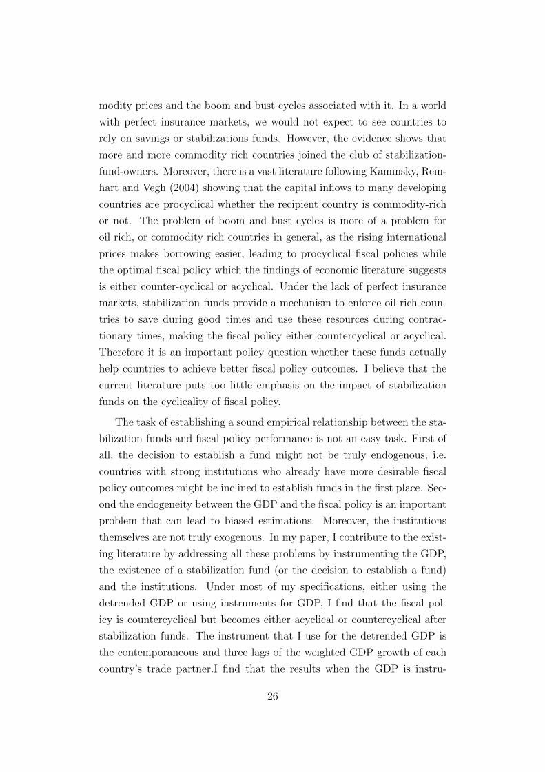
modity prices and the boom and bust cycles associated with it. In a world

with perfect insurance markets, we would not expect to see countries to

rely on savings or stabilizations funds. However, the evidence shows that

more and more commodity rich countries joined the club of stabilization-

fund-owners. Moreover, there is a vast literature following Kaminsky, Rein-

hart and Vegh (2004) showing that the capital inflows to many developing

countries are procyclical whether the recipient country is commodity-rich

or not. The problem of boom and bust cycles is more of a problem for

oil rich, or commodity rich countries in general, as the rising international

prices makes borrowing easier, leading to procyclical fiscal policies while

the optimal fiscal policy which the findings of economic literature suggests

is either counter-cyclical or acyclical. Under the lack of perfect insurance

markets, stabilization funds provide a mechanism to enforce oil-rich coun-

tries to save during good times and use these resources during contrac-

tionary times, making the fiscal policy either countercyclical or acyclical.

Therefore it is an important policy question whether these funds actually

help countries to achieve better fiscal policy outcomes. I believe that the

current literature puts too little emphasis on the impact of stabilization

funds on the cyclicality of fiscal policy.

The task of establishing a sound empirical relationship between the sta-

bilization funds and fiscal policy performance is not an easy task. First of

all, the decision to establish a fund might not be truly endogenous, i.e.

countries with strong institutions who already have more desirable fiscal

policy outcomes might be inclined to establish funds in the first place. Sec-

ond the endogeneity between the GDP and the fiscal policy is an important

problem that can lead to biased estimations. Moreover, the institutions

themselves are not truly exogenous. In my paper, I contribute to the exist-

ing literature by addressing all these problems by instrumenting the GDP,

the existence of a stabilization fund (or the decision to establish a fund)

and the institutions. Under most of my specifications, either using the

detrended GDP or using instruments for GDP, I find that the fiscal pol-

icy is countercyclical but becomes either acyclical or countercyclical after

stabilization funds. The instrument that I use for the detrended GDP is

the contemporaneous and three lags of the weighted GDP growth of each

country’s trade partner.I find that the results when the GDP is instru-

26

mented are similar to OLS estimations. Running seperate estimations for

countries with oil fund only shows that the procyclicality result statistically

dissappears.

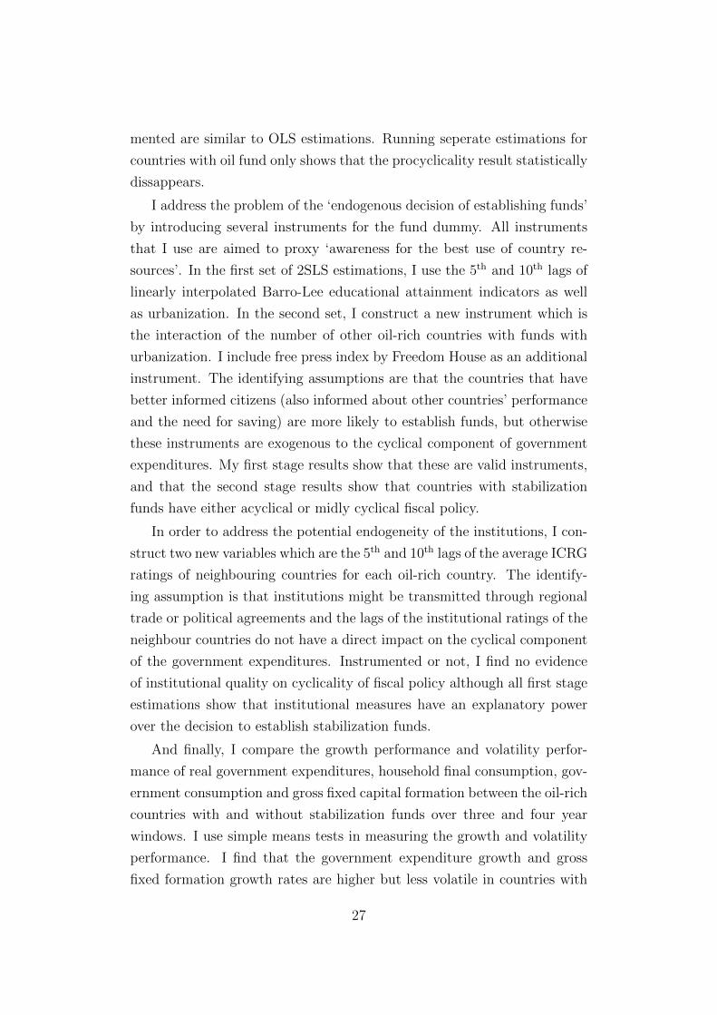
I address the problem of the ‘endogenous decision of establishing funds’

by introducing several instruments for the fund dummy. All instruments

that I use are aimed to proxy ‘awareness for the best use of country re-

sources’. In the first set of 2SLS estimations, I use the 5th and 10th lags of

linearly interpolated Barro-Lee educational attainment indicators as well

as urbanization. In the second set, I construct a new instrument which is

the interaction of the number of other oil-rich countries with funds with

urbanization. I include free press index by Freedom House as an additional

instrument. The identifying assumptions are that the countries that have

better informed citizens (also informed about other countries’ performance

and the need for saving) are more likely to establish funds, but otherwise

these instruments are exogenous to the cyclical component of government

expenditures. My first stage results show that these are valid instruments,

and that the second stage results show that countries with stabilization

funds have either acyclical or midly cyclical fiscal policy.

In order to address the potential endogeneity of the institutions, I con-

struct two new variables which are the 5th and 10th lags of the average ICRG

ratings of neighbouring countries for each oil-rich country. The identify-

ing assumption is that institutions might be transmitted through regional

trade or political agreements and the lags of the institutional ratings of the

neighbour countries do not have a direct impact on the cyclical component

of the government expenditures. Instrumented or not, I find no evidence

of institutional quality on cyclicality of fiscal policy although all first stage

estimations show that institutional measures have an explanatory power

over the decision to establish stabilization funds.

And finally, I compare the growth performance and volatility perfor-

mance of real government expenditures, household final consumption, gov-

ernment consumption and gross fixed capital formation between the oil-rich

countries with and without stabilization funds over three and four year

windows. I use simple means tests in measuring the growth and volatility

performance. I find that the government expenditure growth and gross

fixed formation growth rates are higher but less volatile in countries with

27

stabilization funds. I find no evidence of a statistically meaningful associa-

tion between household final consumption and existence of a stabilization

fund.

In sum, I find that the countries with stabilization funds have fiscal pol-

icy performances with more desirable cyclical properties that are in parallel

with the prescriptions of the optimal fiscal policy literature. However, there

is a clear divide in results when I consider the whole sample or exclude the

countries without funds. The countries which adopted such funds seem to

have less procyclical fiscal policies before and after as opposed to countries

without funds for the whole sample period although degree of procyclicality

seem to decline further after the establishment of the funds. This finding

might suggest that stabilization funds per se are no magic tools and a cer-

tain degree of prudence is needed to achieve more desirable fiscal outcomes

as opposed to the view that such funds necessarily tie the hands of the

governments which cannot impose discipline otherwise. This is in line with

the evidence by Frankel et al. (2012) which suggests that those countries

which graduated from fiscal procyclicality into counter or acyclicality are

the ones with better institutions.

28

5 References

1. Acemoglu, Daron, Simon Johnson and James A. Robinson. 2001.

“The Colonial Origins of Comparative Development: An Empirical Inves-

tigation”. American Economic Review. 91(5): 1369-1401.

2. Angrist, Joshua D. and Jorn-Steffen Pischke. 2009. Mostly Harmless

Econometrics: An Empiricist’s Companion. Princeton: Princeton Univer-

sity Press.

3. Arellano, Manuel and Stephen Bond. 1991. “Some Tests of Spec-

ification for Panel Data: Monte Carlo Evidence and an Application to

Employment Equations”. Review of Economic Studies. 58(April): 277-97.

4. Arrau, Patricio and Stijn Claessens. 1992. “Commodity Stabiliza-

tion Funds”. Policy Research Working Paper Series, No. 835. World Bank,

Washington, D.C.

5. Barnett, Steven and Alvaro Vivanco. 2003. “Statistical Properties of

Oil Prices: Implications for Calculating Government Wealth” in Fiscal Pol-

icy Formation and Implementation in Oil-Producing Countries edited by

Jeffrey M. Davis, Rolando Ossowoski and Annalisa Fedelino. Washington

D.C: International Monetary Fund.

6. Barro, Robert. and Jong-Wha Lee. 2010. “A New Data Set of

Educational Attainment in the World, 1950-2010”. Working Paper, No.

15902, National Bureau of Economic Research, Cambridge, MA.

7. Bartsch, Ulrich. 2006. “How much is Enough? Monte Carlo Sim-

ulations of an Oil Stabilization Fund for Nigeria”. Working Paper, No:

06/142. International Monetary Fund, Washington, D.C.

8. Baum, Christopher F. Mark E. Schaffer and Steven Stillman. 2010.

“Ivreg2: Stata module for extended instrumental variables/2SLS, GMM

and AC/HAC, LIML and k-class regression.” Accessed December 21, 2015.

http://ideas.repec.org/c/boc/bocode/s425401.html

9. Cashin, Paul, Hong Liang and John McDermott. 2000. “How Per-

sistent Are Shocks to World Commodity Prices?”. Staff Paper, No: 47(2).

December. International Monetary Fund, Washington, D.C.

10. Collier, Paul, Rick Van Der Ploeg, Michael Spence and Anthony

J. Venables. 2010. “Managing Resource Revenues in Developing Coun-

tries”. Staff Paper, No: 57(1). October. International Monetary Fund,

29

Washington, D.C.

11. Das, S. Udaibir, Yinquiu Lu, Christian Mulder and Sy Amadou.

2009 “Setting up a Sovereign Wealth Fund: Some Policy and Operational

Considerations” Working Paper, No: 09/179. August. International Mon-

etary Fund, Washington, D.C.

12. Devlin, Julia and Sheridan Titman. 2004. “Managing Oil Price

Risk in Developing Countries”. The World Bank Research Observer. 19(1)

Spring. World Bank, Washington, D.C.

13. Engel, Eduardo, and Rodrigo Valdes. 2000. “Optimal Fiscal Strat-

egy for Mineral Exporting Countries”. Working Paper No: 00/118. June.

International Monetary Fund, Washington, D.C.

14. Fasano, Ugo. 2000 “Review of the Experience with Oil Stabilization

and Savings Funds in Selected Countries”. Working Paper, No: 00/112.

June. International Monetary Fund, Washington, D.C.

15. Frankel, Jeffrey. 2010. “The Natural Resource Curse: A Survey”,

Working Paper, No. 15836, National Bureau of Economic Research, Cam-

bridge, MA.

16. Frankel, Jeffrey, Carlos Vegh and Guillermo Vuletin. 2012. “On

Graduation from Fiscal Procyclicality”.Journal of Development Economics

100(1): 32-47.

17. Freedom House, Freedom of Press Surveys. Accessed January 5,

2015. http://www.freedomhouse.org/template.cfm?page=1

18. Gavin, Michael and Roberto Perotti. 1997 “Fiscal Policy in Latin

America”. NBER Macroeconomics Annual 12: 11-72. National Bureau of

Economic Research, Cambridge, MA.

19. Hausmann, Ricardo and Roberto Rigobon. 2002. “An Alternative

Interpretation of the Resource Curse: Theory and Implications” Working

Paper, No. 9424, National Bureau of Economic Research, Cambridge, MA.

20. Husain, Aasim M., Kamilya Tazhibayeva and Anna Ter-Martirosyan.

2008. “Fiscal Policy and Economic Cycles in Oil-Exporting Countries”

Working Paper, No: 08/253. November. International Monetary Fund,

Washington, D.C.

21. Ilzetzki, Ethan. 2011. “Rent-seeking Distortions and Fiscal Pro-

cyclicality”. Journal of Development Economics 96(1):30-46.

22. Ilzetzki, Ethan and Carlos A. Vegh. 2008. “Procyclical Fiscal

30

Policy in Developing Countries: Truth or Fiction”. Working Paper, No.

14191, National Bureau of Economic Research, Cambridge, MA.

23. International Working Group on Sovereign Wealth Funds. 2008.

“Sovereign Wealth Funds, Generally Accepted Principles and Practices-

Santiago Principles”. Accessed December 21, 2015.

www.iwg-swf.org/pubs/eng/santiagoprinciples.pdf

24. International Monetary Fund. 2012. World Economic Outlook.

Edition: October 2012. ESDS International, University of Manchester.

DOI: http://dx.doi.org/10.5257/imf/weo/201210

25. International Monetary Fund. 2013. Direction of Trade Statistics.

Edition: June 2013. Mimas, University of Manchester.

DOI: http://dx.doi.org/10.5257/imf/dots/2013-06

26. Jaimovich, Dany and Ugo Panizza. 2007. “Procyclicality or Reverse

Causality?” Working Paper, No:599. March. Inter-American Development

Bank, Washington, D.C.

27. Kaminsky, Graciela L., Carmen M. Reinhart and Carlos A. Vegh.

2004. “When It Rains, It Pours: Procyclical Capital Flows and Macroeco-

nomic Policies”. Working Paper, No. 10780, National Bureau of Economic

Research, Cambridge, MA.

28. Ossowski, Rolando, Mauricio Villafuerte, Paolo A. Medas and Theo

Thomas. 2008. “Managing the Oil Revenue Boom: The Role of Fiscal In-

stitutions” Occasional Paper Series, No:260. April. International Monetary

Fund, Washington, D.C.

29. PRS Group. 2013. “International Country Risk Guide Researchers

Dataset” http://www.prsgroup.com/ICRG.aspx

30. Pyndick, Robert S. 1999. “The Long-run Evolution of Energy

Prices”. Energy Journal 20(2): 1-27.

31. Shabsigh, Giath and Nadeem Ilahi. 2007. “Looking Beyond the

Fiscal: Do Oil Funds Bring Macroeconomic Stability?” Working Paper,

No: 07/96. April. International Monetary Fund, Washington, D.C.

32. Sovereign Wealth Fund Institute. 2015. “SWF Rankings”. Ac-

cessed December 7, 2015. http://www.swfinstitute.org/fund-rankings/

33. Vegh, Carlos A and Guillermo Vuletin. 2013. “Tax policy procycli-

cality”. Accessed January 5, 2014. http://www.voxeu.org/article/tax-policy-

procyclicality

31

Tab

le1:

Lis

tof

Cou

ntr

ies

Countr

ySta

biliz

ati

on

F.

Savin

gF

.N

am

eIn

cepti

on

Natu

ral

Reso

urc

e

Alg

eri

a1

0R

evenue

Regula

tion

Fund

2000

oil

Azerb

aij

an

11

Sta

teO

ilFund

1999

oil

Bahra

in1

0R

ese

rve

Fund

for

Str

ate

gic

Pro

jects

2000

oil

Chad

01

Fund

for

Futu

reG

enera

tions

1999-2

006

oil

Ecuador

10

Oil

Sta

biliz

ati

on

Fund

1999

oil

Gab

on

01

Fund

for

Futu

reG

enera

tions

1998

oil

Iran

10

Oil

Sta

biliz

ati

on

Fund

2000

oil

Kazakhst

an

11

Kazakhst

an

Nati

onal

Fund

2001

oil

Kuw

ait

11

KIA

1960

oil

Lib

ya

11

LIA

/O

ilR

ese

rve

Fund

(repla

ced

in2006)

1995

oil

Mexic

o1

1O

ilSta

biliz

ati

on

Fund

2000

oil

Nig

eri

a1

0E

xcess

Cru

de

Account

2004

oil

Norw

ay

11

The

Govern

ment

Pensi

on

Fund

of

Norw

ay

1990

oil

Om

an

01

Sta

teG

enera

lR

ese

rve

Fund

1980

oil

and

gas

Qata

r1

1Q

IA/Sta

biliz

ati

on

Fund

(repla

ced

in2005)

2000

oil

Russ

ia1

0N

ati

onal

Welf

are

Fund/O

ilSta

biliz

ati

on

Fund

(repla

ced

in2008)

2004

oil

Saudi

Ara

bia

01

SA

MA

Fore

ign

Hold

ings

1952

oil

Sudan

10

Oil

Savin

gA

ccount

2002

oil

Tri

nid

ad

and

Tobago

11

Heri

tage

and

Sta

biliz

ati

on

Fund/In

teri

mR

ev.S

tab.

Fund

(repla

ced

in2007)

2000

oil

Venezuela

10

FE

M1999

oil

UA

E0

1A

DIA

1976

oil

Angola

00

--

oil

Bra

zil

00

--

oil

Bolivia

00

--

oil

and

gas

Cam

ero

on

00

--

oil

Republic

of

Congo

00

--

oil

Indonesi

a0

0-

-oil

Vie

tnam

00

--

oil

Yem

en

00

--

oil

Note

:W

eexclu

de

Bru

nei,

Equato

rial

Guin

ea,

and

Tim

or-

Lest

efr

om

the

list

32

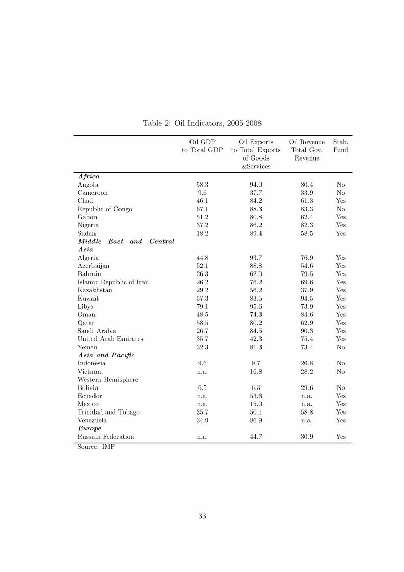
Table 2: Oil Indicators, 2005-2008

Oil GDP Oil Exports Oil Revenue Stab.to Total GDP to Total Exports Total Gov. Fund

of Goods Revenue&Services

AfricaAngola 58.3 94.0 80.4 NoCameroon 9.6 37.7 33.9 NoChad 46.1 84.2 61.3 YesRepublic of Congo 67.1 88.3 83.3 NoGabon 51.2 80.8 62.4 YesNigeria 37.2 86.2 82.3 YesSudan 18.2 89.4 58.5 YesMiddle East and CentralAsiaAlgeria 44.8 93.7 76.9 YesAzerbaijan 52.1 88.8 54.6 YesBahrain 26.3 62.0 79.5 YesIslamic Republic of Iran 26.2 76.2 69.6 YesKazakhstan 29.2 56.2 37.9 YesKuwait 57.3 83.5 94.5 YesLibya 79.1 95.6 73.9 YesOman 48.5 74.3 84.6 YesQatar 58.5 80.2 62.9 YesSaudi Arabia 26.7 84.5 90.3 YesUnited Arab Emirates 35.7 42.3 75.4 YesYemen 32.3 81.3 73.4 NoAsia and PacificIndonesia 9.6 9.7 26.8 NoVietnam n.a. 16.8 28.2 NoWestern HemisphereBolivia 6.5 6.3 29.6 NoEcuador n.a. 53.6 n.a. YesMexico n.a. 15.0 n.a. YesTrinidad and Tobago 35.7 50.1 58.8 YesVenezuela 34.9 86.9 n.a. YesEuropeRussian Federation n.a. 44.7 30.9 Yes

Source: IMF

33

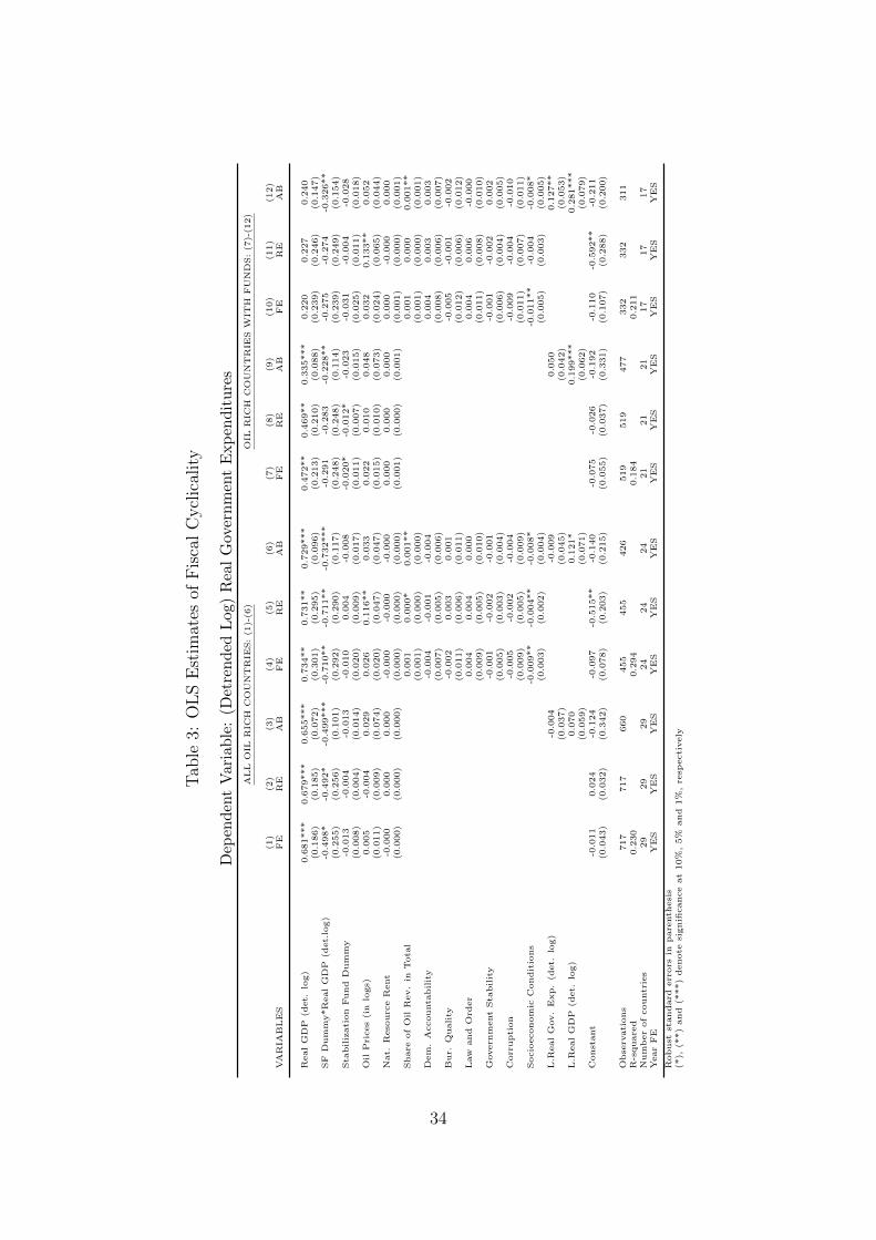
Tab

le3:

OL

SE

stim

ates

ofF

isca

lC

ycl

ical

ity

Dep

end

ent

Var

iab

le:

(Det

ren

ded

Log

)R

eal

Gov

ern

men

tE

xp

end

itu

res

AL

LO

ILR

ICH

CO

UN

TR

IES:

(1)-

(6)

OIL

RIC

HC

OU

NT

RIE

SW

ITH

FU

ND

S:

(7)-

(12)

(1)

(2)

(3)

(4)

(5)

(6)

(7)

(8)

(9)

(10)

(11)

(12)

VA

RIA

BL

ES

FE

RE

AB

FE

RE

AB

FE

RE

AB

FE

RE

AB

Real

GD

P(d

et.

log)

0.6

81***

0.6

79***

0.6

55***

0.7

34**

0.7

31**

0.7

29***

0.4

72**

0.4

69**

0.3

35***

0.2

20

0.2

27

0.2

40

(0.1

86)

(0.1

85)

(0.0

72)

(0.3

01)

(0.2

95)

(0.0

96)

(0.2

13)

(0.2

10)

(0.0

88)

(0.2

39)

(0.2

46)

(0.1

47)

SF

Dum

my*R

eal

GD

P(d

et.

log)

-0.4

98*

-0.4

92*

-0.4

99***

-0.7

10**

-0.7

11**

-0.7

32***

-0.2

91

-0.2

83

-0.2

28**

-0.2

75

-0.2

74

-0.3

26**

(0.2

55)

(0.2

56)

(0.1

01)

(0.2

92)

(0.2

90)

(0.1

17)

(0.2

48)

(0.2

48)

(0.1

14)

(0.2

39)

(0.2

49)

(0.1

54)

Sta

biliz

ati

on

Fund

Dum

my

-0.0

13

-0.0

04

-0.0

13

-0.0

10

0.0

04

-0.0

08

-0.0

20*

-0.0

12*

-0.0

23

-0.0

31

-0.0

04

-0.0

28

(0.0

08)

(0.0

04)

(0.0

14)

(0.0

20)

(0.0

09)

(0.0

17)

(0.0

11)

(0.0

07)

(0.0

15)

(0.0

25)

(0.0

11)

(0.0

18)

Oil

Pri

ces

(in

logs)

0.0

05

-0.0

04

0.0

29

0.0

26

0.1

16**

0.0

33

0.0

22

0.0

10

0.0

48

0.0

32

0.1

33**

0.0

52

(0.0

11)

(0.0

09)

(0.0

74)

(0.0

20)

(0.0

47)

(0.0

47)

(0.0

15)

(0.0

10)

(0.0

73)

(0.0

24)

(0.0

65)

(0.0

44)

Nat.

Reso

urc

eR

ent

-0.0

00

0.0

00

0.0

00

-0.0

00

-0.0

00

-0.0

00

0.0

00

0.0

00

0.0

00

0.0

00

-0.0

00

0.0

00

(0.0

00)

(0.0

00)

(0.0

00)

(0.0

00)

(0.0

00)

(0.0

00)

(0.0

01)

(0.0

00)

(0.0

01)

(0.0

01)

(0.0

00)

(0.0

01)

Share

of

Oil

Rev.

inT

ota

l0.0

01

0.0

00*

0.0

01**

0.0

01

0.0

00

0.0

01**

(0.0

01)

(0.0

00)

(0.0

00)

(0.0

01)

(0.0

00)

(0.0

01)

Dem

.A

ccounta

bilit

y-0

.004

-0.0

01

-0.0

04

0.0

04

0.0

03

0.0

03

(0.0

07)

(0.0

05)

(0.0

06)

(0.0

08)

(0.0

06)

(0.0

07)

Bur.

Quality

-0.0

02

0.0

03

0.0

01

-0.0

05

-0.0

01

-0.0

02

(0.0

11)

(0.0

06)

(0.0

11)

(0.0

12)

(0.0

06)

(0.0

12)

Law

and

Ord

er

0.0

04

0.0

04

0.0

00

0.0

04

0.0

06

-0.0

00

(0.0

09)

(0.0

05)

(0.0

10)

(0.0

11)

(0.0

08)

(0.0

10)

Govern

ment

Sta

bilit

y-0

.001

-0.0

02

-0.0

01

-0.0

01

-0.0

02

0.0

02

(0.0

05)

(0.0

03)

(0.0

04)

(0.0

06)

(0.0

04)

(0.0

05)

Corr

upti

on

-0.0

05

-0.0

02

-0.0

04

-0.0

09

-0.0

04

-0.0

10

(0.0

09)

(0.0

05)

(0.0

09)

(0.0

11)

(0.0

07)

(0.0

11)

Socio

econom

icC

ondit

ions

-0.0

09**

-0.0

04**

-0.0

08*

-0.0

11**

-0.0

04

-0.0

08*

(0.0

03)

(0.0

02)

(0.0

04)

(0.0

05)

(0.0

03)

(0.0

05)

L.R

eal

Gov.

Exp.

(det.

log)

-0.0

04

-0.0

09

0.0

50

0.1

27**

(0.0

37)

(0.0

45)

(0.0

42)

(0.0

53)

L.R

eal

GD

P(d

et.

log)

0.0

70

0.1

21*

0.1

99***

0.2

81***

(0.0

59)

(0.0

71)

(0.0

62)

(0.0

79)

Const

ant

-0.0

11

0.0

24

-0.1

24

-0.0

97

-0.5

15**

-0.1

40

-0.0

75

-0.0

26

-0.1

92

-0.1

10

-0.5

92**

-0.2

11

(0.0

43)

(0.0

32)

(0.3

42)

(0.0

78)

(0.2

03)

(0.2

15)

(0.0

55)

(0.0

37)

(0.3

31)

(0.1

07)

(0.2

88)

(0.2

00)

Obse

rvati

ons

717

717

660

455

455

426

519

519

477

332

332

311

R-s

quare

d0.2

30

0.2

94

0.1

84

0.2

11

Num

ber

of

countr

ies

29

29

29

24

24

24

21

21

21

17

17

17

Year

FE

YE

SY

ES

YE

SY

ES

YE

SY

ES

YE

SY

ES

YE

SY

ES

YE

SY

ES

Robust

standard

err

ors

inpare

nth

esi

s(*

),(*

*)

and

(***)

denote

signifi

cance

at

10%

,5%

and

1%

,re

specti

vely

34

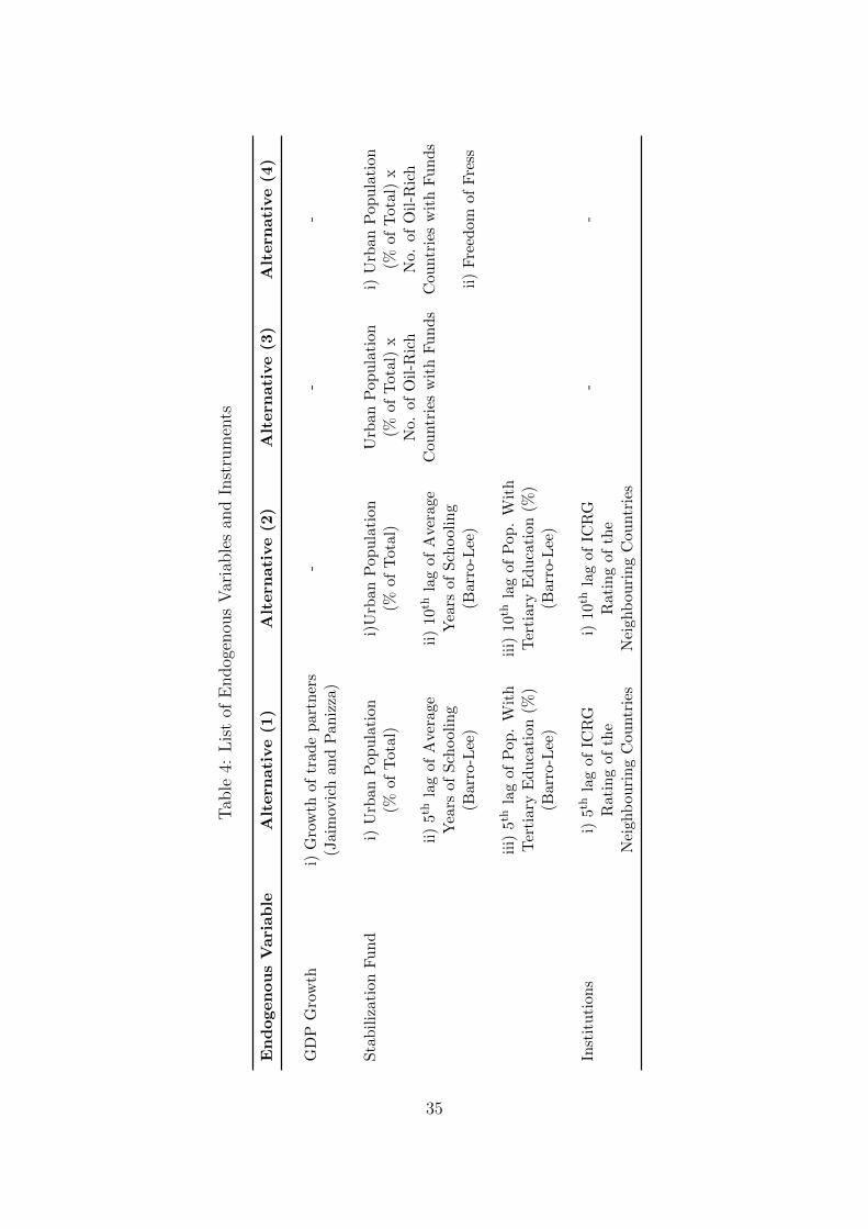
Tab

le4:

Lis

tof

Endog

enou

sV

aria

ble

san

dIn

stru

men

ts

En

dogen

ou

sV

ari

ab

leA

ltern

ati

ve

(1)

Alt

ern

ati

ve

(2)

Alt

ern

ati

ve

(3)

Alt

ern

ati

ve

(4)

GD

PG

row

thi)

Gro

wth

of

trad

ep

artn

ers

--

-(J

aim

ovic

han

dP

aniz

za)

Sta

bil

izat

ion

Fu

nd

i)U

rban

Pop

ula

tion

i)U

rban

Pop

ula

tion

Urb

anP

opu

lati

oni)

Urb

anP

opu

lati

on(%

of

Tot

al)

(%of

Tot

al)

(%of

Tot

al)

x(%

ofT

otal

)x

No.

ofO

il-R

ich

No.

ofO

il-R

ich

ii)

5th

lag

ofA

vera

geii

)10

thla

gof

Ave

rage

Cou

ntr

ies

wit

hF

un

ds

Cou

ntr

ies

wit

hF

un

ds

Yea

rsof

Sch

ool

ing

Yea

rsof

Sch

ool

ing

(Barr

o-L

ee)

(Bar

ro-L

ee)

ii)

Fre

edom

ofF

ress

iii)

5th

lag

of

Pop

.W

ith

iii)

10th

lag

ofP

op.

Wit

hT

erti

ary

Ed

uca

tion

(%)

Ter

tiar

yE

du

cati

on(%

)(B

arr

o-L

ee)

(Bar

ro-L

ee)

Inst

itu

tion

si)

5thla

gof

ICR

Gi)

10th

lag

ofIC

RG

--

Rati

ng

ofth

eR

atin

gof

the

Nei

ghb

ou

rin

gC

ountr

ies

Nei

ghb

ouri

ng

Cou

ntr

ies

35

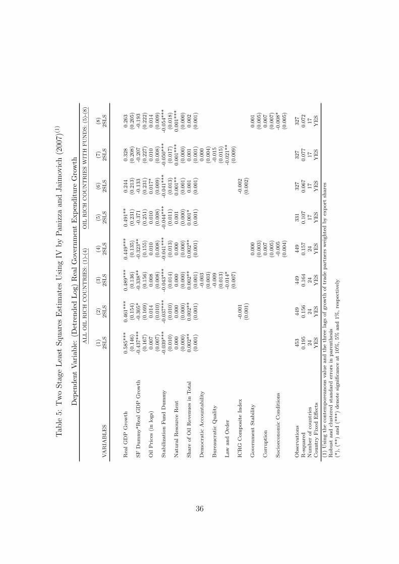
Tab

le5:

Tw

oSta

geL

east

Squar

esE

stim

ates

Usi

ng

IVby

Pan

izza

and

Jai

mov

ich

(200

7)(1

)

Dep

end

ent

Var

iab

le:

(Det

ren

ded

Log

)R

eal

Gov

ern

men

tE

xp

end

itu

reG

row

th

AL

LO

ILR

ICH

CO

UN

TR

IES

:(1

)-(4

)O

ILR

ICH

CO

UN

TR

IES

WIT

HF

UN

DS

:(5

)-(8

)

(1)

(2)

(3)

(4)

(5)

(6)

(7)

(8)

VA

RIA

BL

ES

2S

LS

2S

LS

2S

LS

2S

LS

2S

LS

2S

LS

2S

LS

2S

LS

Rea

lG

DP

Gro

wth

0.5

85***

0.4

61***

0.4

89***

0.4

49***

0.4

91**

0.2

44

0.3

28

0.2

63

(0.1

46)

(0.1

54)

(0.1

36)

(0.1

35)

(0.2

31)

(0.2

13)

(0.2

08)

(0.2

05)

SF

Du

mm

y*R

eal

GD

PG

row

th-0

.437***

-0.3

05*

-0.3

38**

-0.3

23**

-0.3

71

-0.1

33

-0.2

07

-0.1

93

(0.1

67)

(0.1

69)

(0.1

56)

(0.1

55)

(0.2

51)

(0.2

31)

(0.2

27)

(0.2

22)

Oil

Pri

ces

(in

logs)

0.0

07

0.0

14

0.0

08

0.0

10

0.0

10

0.0

17*

0.0

10

0.0

14

(0.0

07)

(0.0

10)

(0.0

08)

(0.0

08)

(0.0

08)

(0.0

09)

(0.0

08)

(0.0

09)

Sta

biliz

ati

on

Fu

nd

Du

mm

y-0

.039***

-0.0

37***

-0.0

43***

-0.0

41***

-0.0

44***

-0.0

41***

-0.0

50***

-0.0

54***

(0.0

10)

(0.0

10)

(0.0

14)

(0.0

13)

(0.0

11)

(0.0

13)

(0.0

17)

(0.0

18)

Natu

ral

Res

ou

rce

Ren

t0.0

00

0.0

00

0.0

00

0.0

00

0.0

01

0.0

01**

0.0

01***

0.0

01***

(0.0

00)

(0.0

00)

(0.0

00)

(0.0

00)

(0.0

00)

(0.0

01)

(0.0

00)

(0.0

00)

Sh

are

of

Oil

Rev

enu

esin

Tota

l0.0

02**

0.0

02**

0.0

02**

0.0

02**

0.0

01*

0.0

01

0.0

01

0.0

02

(0.0

01)

(0.0

01)

(0.0

01)

(0.0

01)

(0.0

01)

(0.0

01)

(0.0

01)

(0.0

01)

Dem

ocr

ati

cA

ccou

nta

bilit

y-0

.003

0.0

00

(0.0

03)

(0.0

04)

Bu

reau

crati

cQ

uality

-0.0

09

-0.0

15

(0.0

13)

(0.0

15)

Law

an

dO

rder

-0.0

14*

-0.0

21**

(0.0

07)

(0.0

09)

ICR

GC

om

posi

teIn

dex

-0.0

01

-0.0

02

(0.0

01)

(0.0

02)

Gover

nm

ent

Sta

bilit

y0.0

00

0.0

01

(0.0

03)

(0.0

05)

Corr

up

tion

0.0

07

0.0

07

(0.0

05)

(0.0

07)

Soci

oec

on

om

icC

on

dit

ion

s-0

.005

-0.0

08*

(0.0

04)

(0.0

05)

Ob

serv

ati

on

s453

449

449

449

331

327

327

327

R-s

qu

are

d0.1

95

0.1

56

0.1

64

0.1

57

0.1

07

0.0

67

0.0

77

0.0

72

Nu

mb

erof

cou

ntr

ies

24

24

24

24

17

17

17

17

Cou

ntr

yF

ixed

Eff

ects

YE

SY

ES

YE

SY

ES

YE

SY

ES

YE

SY

ES

(1)

Usi

ng

the

conte

mp

ore

anou

svalu

ean

dth

eth

ree

lags

of

gro

wth

of

trad

ep

art

ner

sw

eighte

dby

exp

ort

share

sR

ob

ust

an

dcl

ust

ered

stan

dard

erro

rsin

pare

nth

esis

(*),

(**)

an

d(*

**)

den

ote

sign

ifica

nce

at

10%

,5%

an

d1%

,re

spec

tivel

y

36

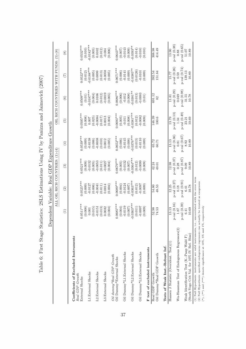
Tab

le6:

Fir

stSta

geSta

tist

ics:

2SL

SE

stim

atio

ns

Usi

ng

IVby

Pan

izza

and

Jai

mov

ich

(200

7)

Dep

end

ent

Var

iab

le:

Rea

lG

DP

Exp

end

itu

reG

row

th

AL

LO

ILR

ICH

CO

UN

TR

IES

:(1

)-(4

)O

ILR

ICH

CO

UN

TR

IES

WIT

HF

UN

DS

:(5

)-(8

)

(1)

(2)

(3)

(4)

(5)

(6)

(7)

(8)

Coeffi

cie

nts

of

Exclu

ded

Inst

ru

ments

RealGDP

Growth

Exte

rnal

Sh

ock

s0.0

511***

0.0

525***

0.0

521***

0.0

539***

0.0

505***

0.0

509***

0.0

522***

0.0

532***

(0.0

08)

(0.0

09)

(0.0

09)

(0.0

09)

(0.0

08)

(0.0

1)

(0.0

12)

(0.0

10)

L1.E

xte

rnal

Sh

ock

s0.0

01

-0.0

127

-0.0

132

-0.0

138

0.0

07

-0.0

187***

-0.0

188***

-0.0

182***

(0.0

15)

(0.0

06)

(0.0

05)

(0.0

06)

(0.0

25)

(0.0

04)

(0.0

05)

(0.0

05)

L2.E

xte

rnal

Sh

ock

s-0

.0151

-0.0

041

-0.0

053

-0.0

038

-0.0

084

0.0

106

0.0

099

0.0

102

(0.0

13)

(0.0

11)

(0.0

11)

(0.0

10)

(0.0

17)

(0.0

12)

(0.0

13)

(0.0

12)

L3.E

xte

rnal

Sh

ock

s0.0

032

0.0

014

-0.0

027

0.0

012

0.0

013

-0.0

019

-0.0

058

-0.0

04

(0.0

04)

(0.0

04)

(0.0

04)

(0.0

05)

(0.0

04)

(0.0

05)

(0.0

05)

(0.0

06)

Oildummy*RealGDP

Growth

Oil

Du

mm

y*E

xte

rnal

Sh

ock

s0.0

685***

0.0

689***

0.0

679***

0.0

652***

0.0

693***

0.0

686***

0.0

671***

0.0

643***

(0.0

04)

(0.0

04)

(0.0

05)

(0.0

06)

(0.0

05)

(0.0

06)

(0.0

06)

(0.0

07)

Oil

Du

mm

y*L

1.E

xte

rnal

Sh

ock

s-0

.0119

-0.0

124

-0.0

132

-0.0

145

-0.0

11

-0.0

12

-0.0

141

-0.0

143

(0.0

07)

(0.0

07)

(0.0

07)

(0.0

08)

(0.0

08)

(0.0

08)

(0.0

09)

(0.0

09)

Oil

Du

mm

y*L

2.E

xte

rnal

Sh

ock

s-0

.0363***

-0.0

363***

-0.0

364***

-0.0

376***

-0.0

381***

-0.0

381**

-0.0

385**

-0.0

393**

(0.0

11)

(0.0

12)

(0.0

12)

(0.0

13)

(0.0

12)

(0.0

13)

(0.0

126)

(0.0

14)

Oil

Du

mm

y*L

3.E

xte

rnal

Sh

ock

s-0

.0097

-0.0

097

-0.0

099

-0.0

110

-0.0

082

-0.0

083

-0.0

101

-0.0

101

(0.0

09)

(0.0

09)

(0.0

09)

(0.0

09)

(0.0

09)

(0.0

1)

(0.0

09)

(0.0

10)

Fte

stof

exclu

ded

inst

ru

ments

Rea

lG

DP

Gro

wth

52.9

854.8

042.2

465.7

2146.3

9691.1

2392.5

4308.9

8O

ilD

um

my*R

eal

GD

PG

row

th74.5

348.5

349.0

160.7

1100.6

82

151.8

4414.4

9

Test

sof

Weak

Inst

.-R

ob

ust

Inf.

Han

sen

JS

tati

stic

(Over

iden

t.T

est)

(1)

13.1

312.2

512.9

813.1

313.7

911.8

115.7

713.9

0p

-val

(0.1

6)

p-v

al

(0.2

7)

p-v

al

(0.3

7)

p-v

al

(0.3

6)

p-v

al

(0.1

3)

p-v

al

(0.2

9)

p-v

al

(0.2

6)

p-v

al

(0.3

8)

Wu

-Hau

sman

Tes

tof

En

dogen

ou

sR

egre

ssors

(2)

1.8

70.1

80.2

80.8

11.3

40.0

49

0.5

90.8

8p

-val

(0.3

9)

p-v

al

(0.9

1)

p-v

al

(0.8

7)

p-v

al

(0.6

7)

p-v

al

(0.4

9)

p-v

al

(0.9

8)

p-v

al

(0.7

4)

p-v

al

(0.6

5)

Wea

kId

enti

fica

tion

Tes

t(K

.-P

aap

Wald

F)

6.4

16.4

19.0

98.9

223.2

131.5

5139.1

351.0

7(S

tock

-Yogo

Cri

tV

al.

for

10%

IVR

el.

Bia

s)10.6

910.7

810.8

910.8

910.6

910.7

810.8

910.8

9

(1)

Null

Hyp

oth

esi

s:in

stru

ments

are

valid

inst

rum

ents

,i.e.,

uncorr

ela

ted

wit

hth

eerr

or

term

(2)

Null

Hyp

oth

esi

s:sp

ecifi

ed

endogenous

regre

ssors

can

actu

ally

be

treate

das

exogenous

(*),

(**)

and

(***)

denote

signifi

cance

at

10%

,5%

and

1%

,re

specti

vely

37

Tab

le7:

Inst

rum

enti

ng

for

the

Intr

oduct

ion

ofth

eSta

biliz

atio

nF

und

Dep

end

ent

Var

iab

le:

(Det

ren

ded

Log

)R

eal

Gov

ern

men

tE

xp

end

itu

res

Inst

rum

ents

:C

olu

mn

s(1

)-(3

)-(5

)-(7

):U

rban

Pop

ula

tion

(%of

tota

l),

5th

Lag

sof

Ave

.Y

ears

ofE

du

cati

onan

dP

opu

lati

onw

ith

Ter

tiar

yE

du

cati

on

(%of

tota

l)C

olu

mn

s(2

)-(4

)-(6

)-(8

):U

rban

Pop

ula

tion

(%of

tota

l),

10th

Lag

sof

Ave

.Y

ears

ofE

du

cati

onan

dP

opu

lati

onw

ith

Ter

tiar

yE

du

cati

on(%

ofto

tal)

AL

LO

ILR

ICH

CO

UN

TR

IES

:(1

)-(4

)O

ILR

ICH

CO

UN

TR

IES

WIT

HF

UN

DS

:(5

)-(8

)

(1)

(2)

(3)

(4)

(5)

(6)

(7)

(8)

VA

RIA

BL

ES

2S

LS

2S

LS

2S

LS

2S

LS

2S

LS

2S

LS

2S

LS

2S

LS

Sta

biliz

ati

on

Fu

nd

Du

mm

y-0

.031

-0.0

57

-0.0

33

-0.0

65

-0.0

51

-0.0

53

-0.0

69

-0.0

77

(0.0

51)

(0.0

60)

(0.0

55)

(0.0

70)

(0.0

53)

(0.0

57)

(0.0

64)

(0.0

74)

Rea

lG

DP

(det

ren

ded

log)

0.4

57***

0.4

29***

0.4

60***

0.4

33***

0.5

02*

0.4

97*

0.5

10*

0.5

01*

(0.1

57)

(0.1

61)

(0.1

52)

(0.1

56)

(0.2

73)

(0.2

85)

(0.2

82)

(0.2

90)

SF

Du

mm

y*R

eal

GD

P(d

etre

nd

edlo

g)

-0.5

08***

-0.4

99**

-0.5

08***

-0.4

97***

-0.5

83**

-0.5

80*

-0.5

57*

-0.5

50*

(0.1

95)

(0.1

95)

(0.1

91)

(0.1

90)

(0.2

94)

(0.2

97)

(0.3

06)

(0.3

08)

Oil

Pri

ces

(in

logs)

0.0

10

0.0

14

0.0

04

0.0

09

0.0

21

0.0

22

0.0

24

0.0

26

(0.0

12)

(0.0

13)

(0.0

13)

(0.0

16)

(0.0

16)

(0.0

17)

(0.0

21)

(0.0

25)

Sh

are

of

Oil

Rev

enu

esin

Tota

l0.0

00

0.0

00

0.0

00

0.0

01

0.0

00

0.0

00

0.0

01

0.0

01

(0.0

01)

(0.0

01)

(0.0

01)

(0.0

01)

(0.0

01)

(0.0

01)

(0.0

01)

(0.0

01)

Natu

ral

Res

ou

rce

Ren

t0.0

01*

0.0

01*

0.0

01

0.0

01

0.0

01*

0.0

01*

0.0

01

0.0

01

(0.0

01)

(0.0

01)

(0.0

01)

(0.0

01)

(0.0

01)

(0.0

01)

(0.0

01)

(0.0

01)

ICR

GC

om

posi

teIn

dex

-0.0

01

-0.0

01

-0.0

01

-0.0

01

(0.0

01)

(0.0

01)

(0.0

01)

(0.0

01)

Dem

ocr

ati

cA

ccou

nta

bilit

y-0

.005

-0.0

05

0.0

02

0.0

02

(0.0

06)

(0.0

06)

(0.0

08)

(0.0

08)

Bu

reau

crati

cQ

uality

-0.0

11

-0.0

14

-0.0

16

-0.0

17

(0.0

12)

(0.0

13)

(0.0

14)

(0.0

14)

Law

an

dO

rder

-0.0

13*

-0.0

13

-0.0

13

-0.0

13

(0.0

08)

(0.0

08)

(0.0

10)

(0.0

10)

Gover

nm

ent

Sta

bilit

y0.0

01

0.0

02

0.0

04

0.0

04

(0.0

04)

(0.0

04)

(0.0

06)

(0.0

06)

Corr

up

tion

0.0

04

0.0

02

-0.0

04

-0.0

05

(0.0

08)

(0.0

09)

(0.0

13)

(0.0

14)

Soci

oec

on

om

icC

on

dit

ion

s0.0

01

0.0

01

-0.0

03

-0.0

04

(0.0

05)

(0.0

05)

(0.0

06)

(0.0

07)

Ob

serv

ati

on

s382

382

382

382

275

275

275

275

R-s

qu

are

d0.0

89

0.0

75

0.0

98

0.0

84

0.0

76

0.0

75

0.0

82

0.0

76

Nu

mb

erof

cou

ntr

ies

20

20

20

20

14

14

14

14

Cou

ntr

yF

ixed

Eff

ects

YE

SY

ES

YE

SY

ES

YE

SY

ES

YE

SY

ES

Rob

ust

an

dcl

ust

ered

stan

dard

erro

rsin

pare

nth

esis

(*),

(**)

an

d(*

**)

den

ote

sign

ifica

nce

at

10%

,5%

an

d1%

,re

spec

tivel

y

38

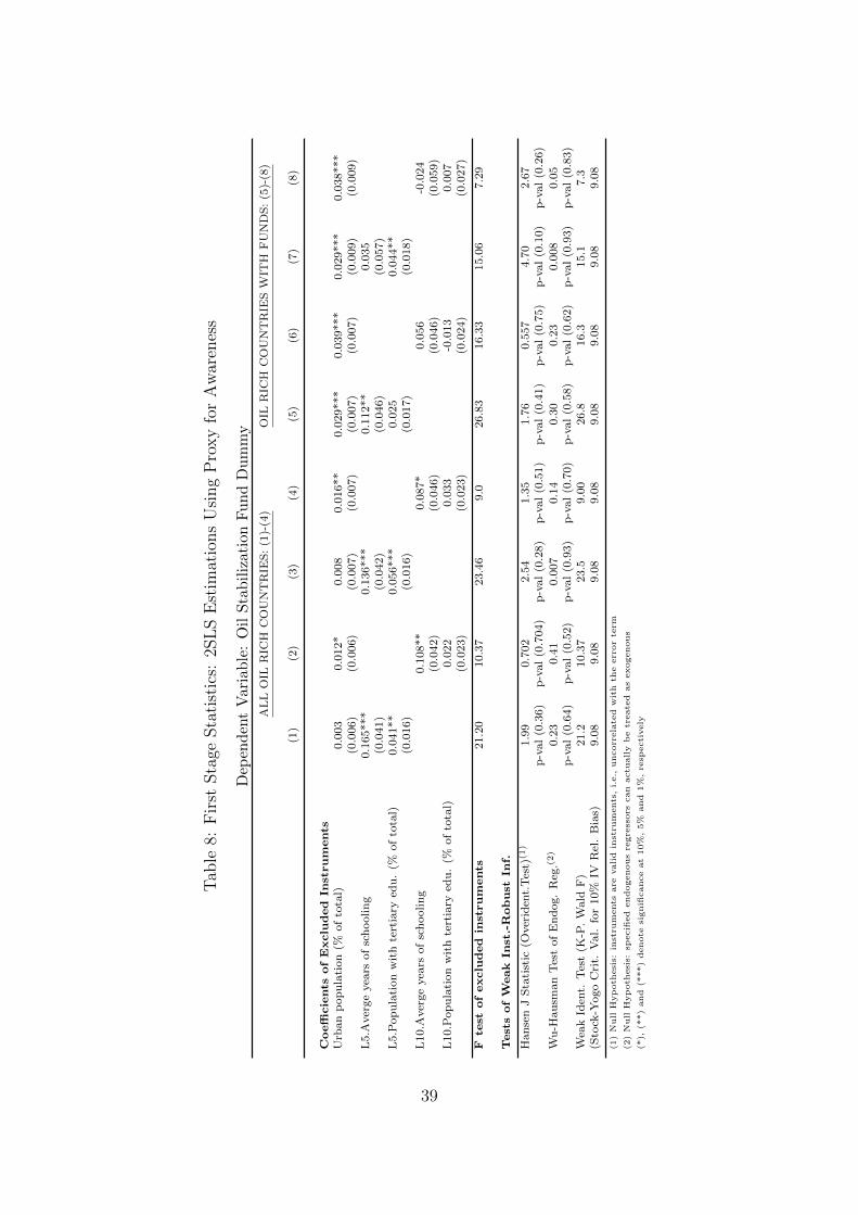
Tab

le8:

Fir

stSta

geSta

tist

ics:

2SL

SE

stim

atio

ns

Usi

ng

Pro

xy

for

Aw

aren

ess

Dep

end

ent

Var

iab

le:

Oil

Sta

bil

izat

ion

Fu

nd

Dum

my

AL

LO

ILR

ICH

CO

UN

TR

IES

:(1

)-(4

)O

ILR

ICH

CO

UN

TR

IES

WIT

HF

UN

DS

:(5

)-(8

)

(1)

(2)

(3)

(4)

(5)

(6)

(7)

(8)

Coeffi

cie

nts

of

Exclu

ded

Inst

ru

ments

Urb

an

pop

ula

tion

(%of

tota

l)0.0

03

0.0

12*

0.0

08

0.0

16**

0.0

29***

0.0

39***

0.0

29***

0.0

38***

(0.0

06)

(0.0

06)

(0.0

07)

(0.0

07)

(0.0

07)

(0.0

07)

(0.0

09)

(0.0

09)

L5.A

ver

ge

yea

rsof

sch

oolin

g0.1

65***

0.1

36***

0.1

12**

0.0

35

(0.0

41)

(0.0

42)

(0.0

46)

(0.0

57)

L5.P

op

ula

tion

wit

hte

rtia

ryed

u.

(%of

tota

l)0.0

41**

0.0

56***

0.0

25

0.0

44**

(0.0

16)

(0.0

16)

(0.0

17)

(0.0

18)

L10.A

ver

ge

yea

rsof

sch

oolin

g0.1

08**

0.0

87*

0.0

56

-0.0

24

(0.0

42)

(0.0

46)

(0.0

46)

(0.0

59)

L10.P

op

ula

tion

wit

hte

rtia

ryed

u.

(%of

tota

l)0.0

22

0.0

33

-0.0

13

0.0

07

(0.0

23)

(0.0

23)

(0.0

24)

(0.0

27)

Fte

stof

exclu

ded

inst

ru

ments

21.2

010.3

723.4

69.0

26.8

316.3

315.0

67.2

9

Test

sof

Weak

Inst

.-R

ob

ust

Inf.

Han

sen

JS

tati

stic

(Over

iden

t.T

est)

(1)

1.9

90.7

02

2.5

41.3

51.7

60.5

57

4.7

02.6

7p

-val

(0.3

6)

p-v

al

(0.7

04)

p-v

al

(0.2

8)

p-v

al

(0.5

1)

p-v

al

(0.4

1)

p-v

al

(0.7

5)

p-v

al

(0.1

0)

p-v

al

(0.2

6)

Wu

-Hau

sman

Tes

tof

En

dog.

Reg

.(2)

0.2

30.4

10.0

07

0.1

40.3

00.2

30.0

08

0.0

5p

-val

(0.6

4)

p-v

al

(0.5

2)

p-v

al

(0.9

3)

p-v

al

(0.7

0)

p-v

al

(0.5

8)

p-v

al

(0.6

2)

p-v

al

(0.9

3)

p-v

al

(0.8

3)

Wea

kId

ent.

Tes

t(K

-P.

Wald

F)

21.2

10.3

723.5

9.0

026.8

16.3

15.1

7.3

(Sto

ck-Y

ogo

Cri

t.V

al.

for

10%

IVR

el.

Bia

s)9.0

89.0

89.0

89.0

89.0

89.0

89.0

89.0

8

(1)

Null

Hyp

oth

esi

s:in

stru

ments

are

valid

inst

rum

ents

,i.e.,

uncorr

ela

ted

wit

hth

eerr

or

term

(2)

Null

Hyp

oth

esi

s:sp

ecifi

ed

endogenous

regre

ssors

can

actu

ally

be

treate

das

exogenous

(*),

(**)

and

(***)

denote

signifi

cance

at

10%

,5%

and

1%

,re

specti

vely

39

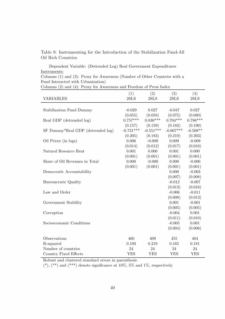
Table 9: Instrumenting for the Introduction of the Stabilization Fund-AllOil Rich Countries

Dependent Variable: (Detrended Log) Real Government ExpendituresInstruments:Columns (1) and (3): Proxy for Awareness (Number of Other Countries with aFund Interacted with Urbanization)Columns (2) and (4): Proxy for Awareness and Freedom of Press Index

(1) (2) (3) (4)VARIABLES 2SLS 2SLS 2SLS 2SLS

Stabilization Fund Dummy -0.029 0.027 -0.047 0.027(0.055) (0.058) (0.075) (0.080)

Real GDP (detrended log) 0.757*** 0.830*** 0.704*** 0.786***(0.157) (0.159) (0.182) (0.190)

SF Dummy*Real GDP (detrended log) -0.731*** -0.551*** -0.667*** -0.508**(0.205) (0.183) (0.210) (0.203)

Oil Prices (in logs) 0.006 -0.009 0.009 -0.009(0.014) (0.012) (0.017) (0.016)

Natural Resource Rent 0.001 0.000 0.001 0.000(0.001) (0.001) (0.001) (0.001)

Share of Oil Revenues in Total 0.000 -0.000 0.000 -0.000(0.001) (0.001) (0.001) (0.001)

Democratic Accountability 0.000 -0.003(0.007) (0.008)

Bureaucratic Quality -0.012 -0.007(0.013) (0.016)

Law and Order -0.006 -0.011(0.008) (0.013)

Government Stability 0.001 -0.001(0.005) (0.005)

Corruption -0.004 0.001(0.011) (0.010)

Socioeconomic Conditions -0.005 0.001(0.004) (0.006)

Observations 460 409 455 404R-squared 0.193 0.219 0.165 0.181Number of countries 24 24 24 24Country Fixed Effects YES YES YES YES

Robust and clustered standard errors in parenthesis(*), (**) and (***) denote significance at 10%, 5% and 1%, respectively

40

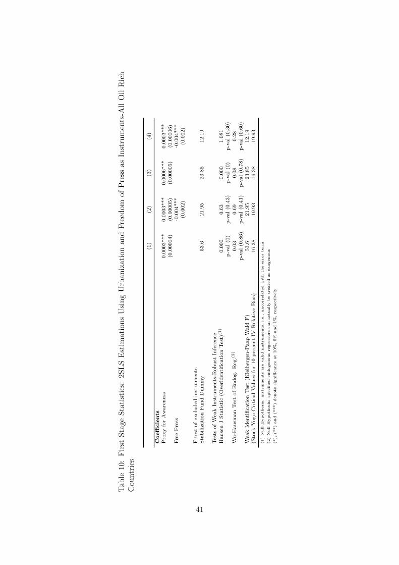
Tab

le10

:F

irst

Sta

geSta

tist

ics:

2SL

SE

stim

atio

ns

Usi

ng

Urb

aniz

atio

nan

dF

reed

omof

Pre

ssas

Inst

rum

ents

-All

Oil

Ric

hC

ountr

ies

(1)

(2)

(3)

(4)

Coeffi

cie

nts

Pro

xy

for

Aw

are

nes

s0.0

003***

0.0

003***

0.0

006***

0.0

003***

(0.0

0004)

(0.0

0005)

(0.0

0005)

(0.0

0006)

Fre

eP

ress

-0.0

04***

-0.0

04***

(0.0

02)

(0.0

02)

Fte

stof

excl

uded

inst

rum

ents

Sta

biliz

ati

on

Fu

nd

Du

mm

y53.6

21.9

523.8

512.1

9

Tes

tsof

Wea

kIn

stru

men

ts-R

ob

ust

Infe

ren

ce

Han

sen

JS

tati

stic

(Over

iden

tifi

cati

on

Tes

t)(1

)0.0

00

0.6

30.0

00

1.0

81

p-v

al

(0)

p-v

al

(0.4

3)

p-v

al

(0)

p-v

al

(0.3

0)

Wu

-Hau

sman

Tes

tof

En

dog.

Reg

.(2)

0.0

30.6

90.0

80.2

8p

-val

(0.8

6)

p-v

al

(0.4

1)

p-v

al

(0.7

8)

p-v

al

(0.6

0)

Wea

kId

enti

fica

tion

Tes

t(K

leib

ergen

-Paap

Wald

F)

53.6

21.9

523.8

512.1

9(S

tock

-Yogo

Cri

tica

lV

alu

esfo

r10

per

cent

IVR

elati

ve

Bia

s)16.3

819.9

316.3

819.9

3

(1)

Null

Hyp

oth

esi

s:in

stru

ments

are

valid

inst

rum

ents

,i.e.,

uncorr

ela

ted

wit

hth

eerr

or

term

(2)

Null

Hyp

oth

esi

s:sp

ecifi

ed

endogenous

regre

ssors

can

actu

ally

be

treate

das

exogenous

(*),

(**)

and

(***)

denote

signifi

cance

at

10%

,5%

and

1%

,re

specti

vely

41

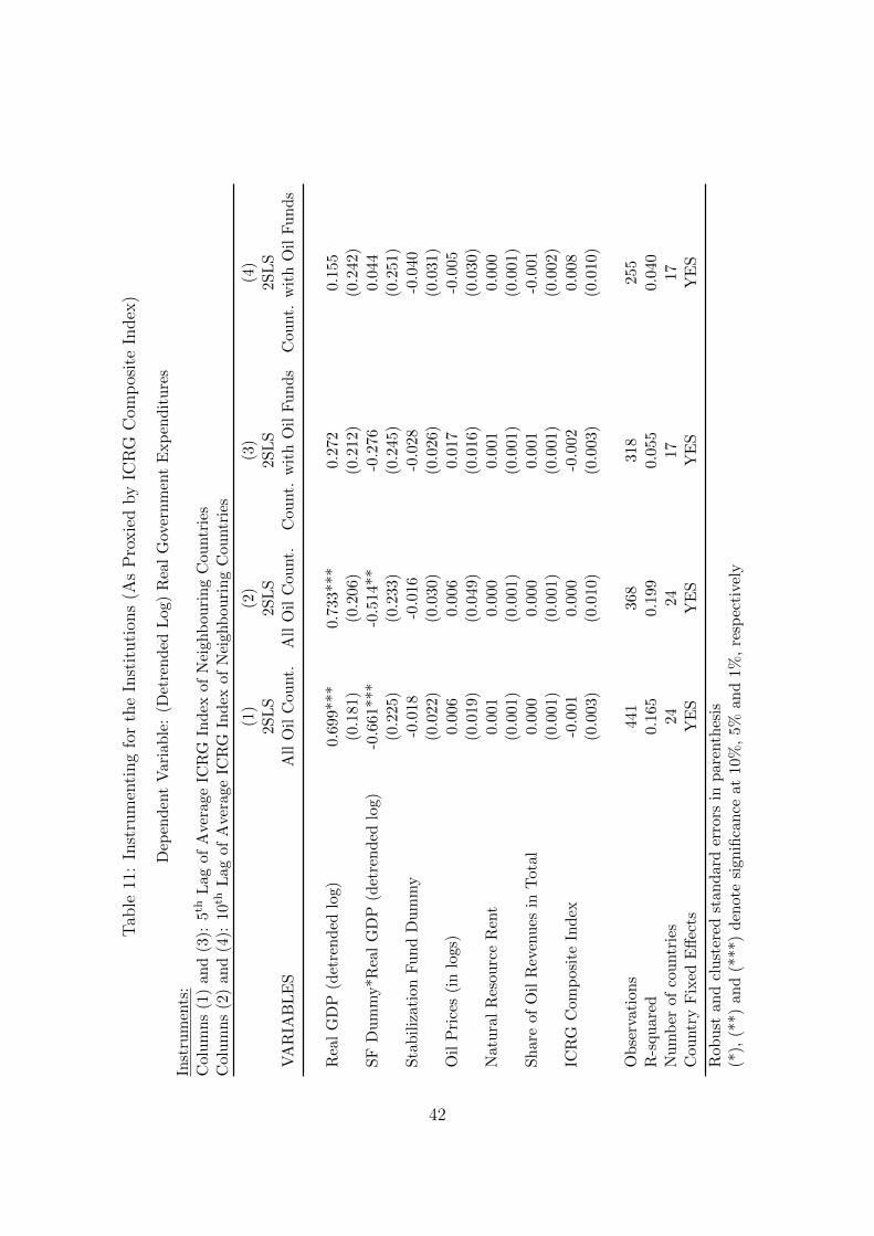
Tab

le11

:In

stru

men

ting

for

the

Inst

ituti

ons

(As

Pro

xie

dby

ICR

GC

omp

osit

eIn

dex

)

Dep

end

ent

Var

iab

le:

(Det

ren

ded

Log

)R

eal

Gov

ern

men

tE

xp

end

itu

res

Inst

rum

ents

:C

olu

mn

s(1

)an

d(3

):5

thL

ag

of

Ave

rage

ICR

GIn

dex

ofN

eigh

bou

rin

gC

ountr

ies

Col

um

ns

(2)

and

(4):

10th

Lag

of

Ave

rage

ICR

GIn

dex

ofN

eigh

bou

rin

gC

ountr

ies

(1)

(2)

(3)

(4)

2SL

S2S

LS

2SL

S2S

LS

VA

RIA

BL

ES

All

Oil

Cou

nt.

All

Oil

Cou

nt.

Cou

nt.

wit

hO

ilF

un

ds

Cou

nt.

wit

hO

ilF

un

ds

Rea

lG

DP

(det

ren

ded

log)

0.69

9***

0.73

3***

0.27

20.

155

(0.1

81)

(0.2

06)

(0.2

12)

(0.2

42)

SF

Du

mm

y*R

eal

GD

P(d

etre

nd

edlo

g)-0

.661

***

-0.5

14**

-0.2

760.

044

(0.2

25)

(0.2

33)

(0.2

45)

(0.2

51)

Sta

bil

izat

ion

Fu

nd

Du

mm

y-0

.018

-0.0

16-0

.028

-0.0

40(0

.022

)(0

.030

)(0

.026

)(0

.031

)O

ilP

rice

s(i

nlo

gs)

0.00

60.

006

0.01

7-0

.005

(0.0

19)

(0.0

49)

(0.0

16)

(0.0

30)

Natu

ral

Res

ou

rce

Ren

t0.

001

0.00

00.

001

0.00

0(0

.001

)(0

.001

)(0

.001

)(0

.001

)S

har

eof

Oil

Rev

enu

esin

Tota

l0.

000

0.00

00.

001

-0.0

01(0

.001

)(0

.001

)(0

.001

)(0

.002

)IC

RG

Com

posi

teIn

dex

-0.0

010.

000

-0.0

020.

008

(0.0

03)

(0.0

10)

(0.0

03)

(0.0

10)

Ob

serv

ati

on

s44

136

831

825

5R

-squ

are

d0.

165

0.19

90.

055

0.04

0N

um

ber

of

cou

ntr

ies

2424

1717

Cou

ntr

yF

ixed

Eff

ects

YE

SY

ES

YE

SY

ES

Rob

ust

an

dcl

ust

ered

stan

dar

der

rors

inp

are

nth

esis

(*),

(**)

an

d(*

**)

den

ote

sign

ifica

nce

at

10%

,5%

and

1%,

resp

ecti

vel

y

42

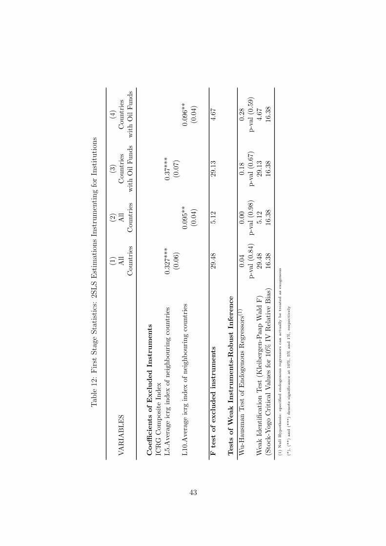
Tab

le12

:F

irst

Sta

geSta

tist

ics:

2SL

SE

stim

atio

ns

Inst

rum

enti

ng

for

Inst

ituti

ons

(1)

(2)

(3)

(4)

VA

RIA

BL

ES

All

All

Cou

ntr

ies

Cou

ntr

ies

Cou

ntr

ies

Cou

ntr

ies

wit

hO

ilF

un

ds

wit

hO

ilF

un

ds

Coeffi

cie

nts

of

Exclu

ded

Inst

rum

ents

ICR

GC

om

posi

teIn

dex

L5.A

vera

ge

icrg

ind

exof

nei

ghb

ouri

ng

countr

ies

0.32

7***

0.37

***

(0.0

6)(0

.07)

L10.

Ave

rage

icrg

ind

exof

nei

ghb

ouri

ng

countr

ies

0.09

5**

0.09

6**

(0.0

4)(0

.04)

Fte

stof

exclu

ded

inst

rum

ents

29.4

85.

1229

.13

4.67

Test

sof

Weak

Inst

rum

ents

-Rob

ust

Infe

ren

ce

Wu

-Hau

sman

Tes

tof

En

dogen

ou

sR

egre

ssor

s(1)

0.04

0.00

0.18

0.28

p-v

al(0

.84)

p-v

al(0

.98)

p-v

al(0

.67)

p-v

al(0

.59)

Wea

kId

enti

fica

tion

Tes

t(K

leib

erge

n-P

aap

Wal

dF

)29

.48

5.12

29.1

34.

67(S

tock

-Yog

oC

riti

cal

Valu

esfo

r10

%IV

Rel

ativ

eB

ias)

16.3

816

.38

16.3

816

.38

(1)

Null

Hyp

oth

esi

s:sp

ecifi

ed

endogenous

regre

ssors

can

actu

ally

be

treate

das

exogenous

(*),

(**)

and

(***)

denote

signifi

cance

at

10%

,5%

and

1%

,re

specti

vely

43

Table 13: Instrumenting for the Real GDP Growth and the StabilizationFund

Dependent Variable: (Detrended Log) Real Government ExpendituresInstruments: External Shocks (Panizza and Jaimovich (2007)) and Proxy For AwarenessColumn (1): ALL OIL RICH COUNTRIESColumn (2): OIL RICH COUNTRIES WITH FUNDS

(1) (2)VARIABLES 2SLS 2SLS

Real GDP Growth 0.670*** 0.543(0.217) (0.613)

SF Dummy*Real GDP Growth -0.625** -0.444(0.286) (0.672)

Stabilization Fund Dummy -0.024 -0.032(0.035) (0.034)

ICRG Composite Index 0.005 0.017(0.008) (0.013)

Oil Prices (in logs) 0.002*** 0.002***(0.001) (0.001)

Natural Resource Rent 0.001 0.001(0.001) (0.001)

Share of Oil Revenues in Total -0.002 -0.002(0.001) (0.002)

Observations 380 273R-squared 0.086 0.100Number of countries 20 14Country Fixed Effects YES YES

Robust and clustered standard errors in parenthesis(*), (**) and (***) denote significance at 10%, 5% and 1%, respectively

44

Tab

le14

:F

irst

Sta

geSta

tist

ics:

Inst

rum

enti

ng

for

the

Rea

lG

DP

Gro

wth

and

the

Sta

biliz

atio

nF

und

Inst

rum

ents

:E

xte

rnal

Sh

ock

s(P

aniz

zaan

dJai

mov

ich

(200

7))

and

Pro

xy

For

Aw

aren

ess

Col

um

n(1

):A

LL

OIL

RIC

HC

OU

NT

RIE

SC

olu

mn

(2):

OIL

RIC

HC

OU

NT

RIE

SW

ITH

FU

ND

S

(1)

(2)

Coeffi

cie

nts

RealGDP

Growth

Exte

rnal

Sh

ock

s0.

0378

0.06

86**

*(0

.023

)(0

.012

)Oildummy

Urb

anp

opu

lati

on(%

ofto

tal)

0.01

280.

0364

*(0

.027

)(0

.018

)L

5.P

op

ula

tion

wit

hte

rtia

ryed

uca

tion

(%of

tota

l)0.

1767

0.33

51**

*(0

.125

)(0

.096

)F

test

of

exclu

ded

inst

rum

ents

Rea

lG

DP

Gro

wth

39.9

118

7.32

Oil

Du

mm

y11

.96

53.1

6

Test

sof

Weak

Inst

rum

ents

-Robu

stIn

fere

nce

Han

sen

JS

tati

stic

(Ove

rid

enti

fica

tion

Tes

t)(1

)11

.08

9.75

p-v

al(0

.35)

p-v

al(0

.46)

Wea

kId

enti

fica

tion

Tes

t(K

leib

erge

n-P

aap

Wal

dF

)3.

316

10.0

9(S

tock

-Yog

oC

riti

cal

Val

ues

for

10%

IVR

elat

ive

Bia

s)10

.14

10.1

4

(1)

Null

Hyp

oth

esi

s:in

stru

ments

are

valid

inst

rum

ents

,i.e.,

uncorr

ela

ted

wit

hth

eerr

or

term

(*),

(**)

and

(***)

denote

signifi

cance

at

10%

,5%

and

1%

,re

specti

vely

45

Table 15: T-tests of Growth Differences

Mean(Fund=1)(1) Mean (Fund=0) Diff.(2)

3 Year Growth

Real Household Final Consumption 0.2015 0.1138 0.0877***(0.0172) (0.0172) (0.0258)

Real Government Final Consumption 0.2423 0.1298 0.1124***(0.0218) (0.0201) (0.0308)

Real Fixed Gross Capital Formation 0.3851 0.1585 0.2266***(0.0449) (0.0237) (0.0464)

Real GDP 0.1601 0.1316 0.0285**(0.0125) (0.0082) (0.0143)

Real General Government Expenditures 0.213 0.1577 0.0553**(0.0201) (0.0176) (0.0272)

Real General Government Revenues 0.2483 0.2106 0.0342(0.0228) (0.0206) (0.0316)

4 Year Growth

Real Household Final Consumption 0.2799 0.1651 0.1148***(0.0227) (0.0203) (0.0319)

Real Government Final Consumption 0.3465 0.1931 0.1535***(0.0306) (0.0245) (0.0398)

Real Fixed Gross Capital Formation 0.5577 0.2282 0.3490***(0.0648) (0.0284) (0.0618)

Real GDP 0.2232 0.1872 0.0359*(0.0169) (0.0108) (0.0191)

Real General Government Expenditures 0.3033 0.2168 0.0865**(0.0260) (0.0218) (0.0347)

Real General Government Revenues 0.3375 0.2984 0.0392(0.0307) (0.0254) (0.0406)

(*), (**) and (***) denote significance at 10%, 5% and 1%, respectively(1)Oil Fund dummy takes on the value 1 in the 3rd year (4th for the second panel) of oil fund(2)Null Hypothesis = Mean Gr.(Fund=1) - Mean Gr.(Fund=0) == 0(3) Data source for cons. and inv. is WDI and for GDP,expenditures and revenues data sources are WEO and IMF Country Desks

46

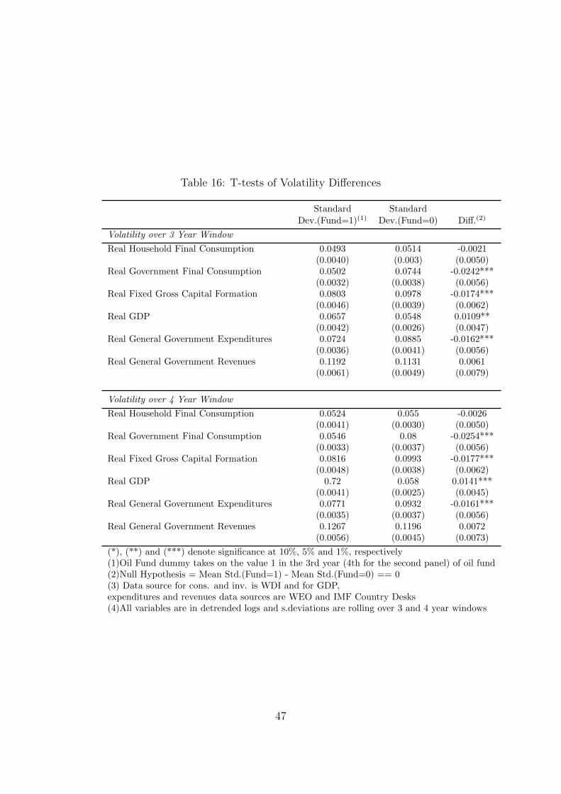
Table 16: T-tests of Volatility Differences

Standard StandardDev.(Fund=1)(1) Dev.(Fund=0) Diff.(2)

Volatility over 3 Year Window

Real Household Final Consumption 0.0493 0.0514 -0.0021(0.0040) (0.003) (0.0050)

Real Government Final Consumption 0.0502 0.0744 -0.0242***(0.0032) (0.0038) (0.0056)

Real Fixed Gross Capital Formation 0.0803 0.0978 -0.0174***(0.0046) (0.0039) (0.0062)

Real GDP 0.0657 0.0548 0.0109**(0.0042) (0.0026) (0.0047)

Real General Government Expenditures 0.0724 0.0885 -0.0162***(0.0036) (0.0041) (0.0056)

Real General Government Revenues 0.1192 0.1131 0.0061(0.0061) (0.0049) (0.0079)

Volatility over 4 Year Window

Real Household Final Consumption 0.0524 0.055 -0.0026(0.0041) (0.0030) (0.0050)

Real Government Final Consumption 0.0546 0.08 -0.0254***(0.0033) (0.0037) (0.0056)

Real Fixed Gross Capital Formation 0.0816 0.0993 -0.0177***(0.0048) (0.0038) (0.0062)

Real GDP 0.72 0.058 0.0141***(0.0041) (0.0025) (0.0045)

Real General Government Expenditures 0.0771 0.0932 -0.0161***(0.0035) (0.0037) (0.0056)

Real General Government Revenues 0.1267 0.1196 0.0072(0.0056) (0.0045) (0.0073)

(*), (**) and (***) denote significance at 10%, 5% and 1%, respectively(1)Oil Fund dummy takes on the value 1 in the 3rd year (4th for the second panel) of oil fund(2)Null Hypothesis = Mean Std.(Fund=1) - Mean Std.(Fund=0) == 0(3) Data source for cons. and inv. is WDI and for GDP,expenditures and revenues data sources are WEO and IMF Country Desks(4)All variables are in detrended logs and s.deviations are rolling over 3 and 4 year windows

47

Table 17: Test of Volatility Differences, Relative to GDP Volatility

Relative RelativeStd.(Fund=1)(1) Std.(Fund=0) Diff.(2)

Volatility over 3 Year Window

Real Household Final Consumption 1.237 1.628 -0.391*(0.1586) (0.1203) (0.1991)

Real Government Final Consumption 1.459 2.582 -1.1245***(0.1331) (0.2182) (0.3050)

Real Fixed Gross Capital Formation 2.251 3.7252 -1.4745***(0.2148) (0.2795) (0.4027)

Real General Government Expenditures 1.9245 2.9251 -1.0006***(0.1732) (0.2618) (0.3637)

Real General Government Revenues 2.5948 3.9150 -1.3202(0.1742) (0.6157) (0.8064)

Volatility over 4 Year Window

Real Household Final Consumption 0.9598 1.1942 -0.2345*(0.1180) (0.0669) (0.1258)

Real Government Final Consumption 1.204 2.0856 -0.8816***(0.1020) (0.1074) (0.1646)

Real Fixed Gross Capital Formation 1.6476 2.8839 -1.2363***(0.1409) (0.164) (0.2475)

Real General Government Expenditures 1.5488 2.3982 -0.8493***(0.1140) (0.1198) (0.1810)

Real General Government Revenues 2.2806 3.2265 -0.9458*(0.1299) (0.3692) (0.5013)

(*), (**) and (***) denote significance at 10%, 5% and 1%, respectively(1)Oil Fund dummy takes on the value 1 in the 3rd year (4th for the second panel) of oil fund(2)Null Hypothesis = Mean of Relative Std.(Fund=1)-Mean of Relative Std.(Fund=0) == 0(3) Data source for cons. and inv. is WDI and for GDP,expenditures and revenues data sources are WEO and IMF Country Desks(4)All variables are in detrended logs and s.deviations are rolling over 3 and 4 year windows

48

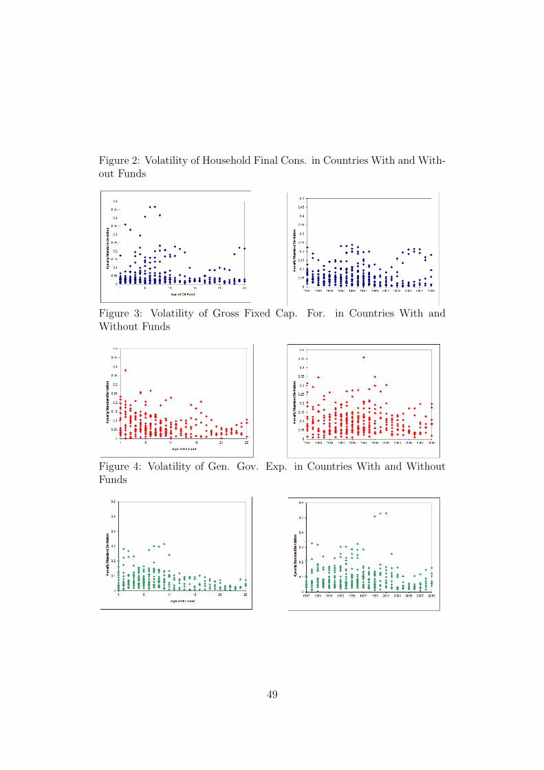
Figure 2: Volatility of Household Final Cons. in Countries With and With-out Funds

Figure 3: Volatility of Gross Fixed Cap. For. in Countries With andWithout Funds

Figure 4: Volatility of Gen. Gov. Exp. in Countries With and WithoutFunds

49

Figure 5: General Government Expenditure Volatility by Country: FundCountries (Right) versus All Countries (Left)

Figure 6: Investment Volatility by Country: Fund Countries (Right) versusAll Countries (Left)

50