Estimating Logit Models with Small Samples∗

Carlisle Rainey‡

Kelly McCaskey†

Abstract

In small samples, maximum likelihood (ML) estimates of logit model coefficients havesubstantial bias away from zero. As a solution, we introduce political scientists toFirth’s (1993) penalized maximum likelihood (PML) estimator. Prior research hasdescribed and used PML, especially in the context of separation, but it’s small sampleproperties remain under-appreciated. The PML estimator eliminates most of the biasand, perhaps more importantly, greatly reduces the variance of the usual ML estimator.Thus, researchers do not face a bias-variance tradeoff when choosing between the MLand PML estimators–the PML estimator has a smaller bias and a smaller variance.We use Monte Carlo simulations and a re-analysis of George and Epstein (1992)to show that the PML estimator offers a substantial improvement in small samples(e.g., 50 observations) and noticeable improvement even in larger samples (e.g., 1,000observations).

∗We thank Tracy George, Lee Epstein, and Alex Weisiger for making their data available. We thank Scott Cook,Soren Jordan, Paul Kellstedt, Dan Wood, and Chris Zorn for helpful comments. We also thank participants at the2015 Annual Meeting of the Society for Political Methodology and a seminar at Texas A&M University for helpfulcomments. We conducted these analyses analyses with R 3.2.2. All data and computer code necessary to reproduceour results are available at github.com/kellymccaskey/small.

‡Carlisle Rainey is Assistant Professor of Political Science, Texas A&M University, 2010 Allen Building, CollegeStation, TX, 77843 (crainey@tamu.edu).

†Kelly McCaskey is Operations Analyst at Accruent, 11500 Alterra Parkway, #110, Austin, TX, 78758 (kmc-caskey@accruent.com).

Logit and probit models have become a staple in quantitative political and social science–

nearly as common as linear regression (Krueger and Lewis-Beck 2008). And while the usual

maximum likelihood (ML) estimates of logit and probit model coefficients have excellent large-

sample properties, these estimates behave quite poorly in small samples. Because the researcher

cannot always collect more data, this raises an important question: How can a researcher obtain

reasonable estimates of logit and probit model coefficients using only a small sample?

In this paper, we introduce political scientists to Firth’s (1993) penalized maximum likelihood

(PML) estimator, which greatly reduces the small-sample bias of ML estimates of logit model

coefficients. We show that the PML estimator nearly eliminates the bias, which can be substantial.

But even more importantly, the PML estimator dramatically reduces the variance of the ML

estimator. Of course, the inflated bias and variance of the ML estimator lead to a larger overall

mean-squared error (MSE). Moreover, we offer Monte Carlo evidence that evidence that the PML

estimator offers a substantial improvement in small samples (e.g., 100 observations) and noticeable

improvement even in large samples (e.g., 1,000 observations).

The Big Problem with Small Samples

When working with a binary outcome yi, the researcher typically models probability of an event,

so that

Pr(yi) = Pr(yi = 1 | Xi) = g−1(Xi β) , (1)

where y represents a vector of binary outcomes, X represents amatrix of explanatory variables and a

constant, β represents a vector of model coefficients, and g−1 represents some inverse-link function

that maps R into [0, 1]. When g−1 represents the inverse-logit function logit−1(α) =1

1 + e−αor the

cumulative normal distribution function Φ(α) =∫ α

−∞

1√2π

e−x22 dx, then we refer to Equation 1 as a

logit or probit model, respectively. To simplify the exposition, we focus on logit models because

the canonical logit link function induces nicer theoretical properties (McCullagh and Nelder 1989,

2

pp. 31-32). In practice, though, Kosmidis and Firth (2009) show that the ideas we discuss apply

equally well to probit models.

To develop the ML estimator of the logit model, we can derive the likelihood function

Pr(y | β) = L(β |y) =n∏

i=1

(1

1 + e−Xi β

) yi (1 −

11 + e−Xi β

)1−yi and, as usual, take the natural logarithm of both sides to obtain the log-likelihood function

log L(β |y) =n∑

i=1

[yi log

(1

1 + e−Xi β

)+ (1 − yi) log

(1 −

11 + e−Xi β

)].

The researcher can obtain the ML estimate β̂mle by finding the vector β that maximizes log L given

y and X (King 1998).1

The ML estimator has excellent properties in large samples. It is asymptotically unbiased, so

that E( β̂mle) ≈ βtrue when the sample is large (Wooldridge 2002, pp. 391-395, and Casella and

Berger 2002, p. 470). It is also asymptotically efficient, so that the asymptotic variance of the ML

estimate obtains the Cramer-Rao lower bound (Greene 2012, pp. 513-523, and Casella and Berger

2002, pp. 472, 516). For small samples, though, the ML estimator of logit model coefficients does

not work well–the ML estimates have substantial bias away from zero (Long 1997, pp. 53-54).

Long (1997, p. 54) offers a rough heuristic about appropriate sample sizes: “It is risky to use

ML with samples smaller than 100, while samples larger than 500 seem adequate.”2 This presents

the researcher with a problem: When dealing with small samples, how can she obtain reasonable

estimates of logit model coefficients?

1In practice, we use iteratively reweighted least squares to use ML to fit logit models in this paper, the defaultbehavior of glm() in R.

2Making the problem worse, King and Zeng (2001) point out that ML estimates have substantial bias for muchlarger sample sizes if the event of interest occurs only rarely.

3

An Easy Solution for the Big Problem

The statistics literature offers a simple solution to the problem of bias. Firth (1993) suggests

penalizing the usual likelihood function L(β |y) by a factor equal to the square root of the determinant

of the information matrix |I (β) |12 , which produces a “penalized” likelihood function L∗(β |y) =

L(β |y) |I (β) |12 (see also Kosmidis and Firth 2009 and Kosmidis 2014).3 It turns out that this

penalty is equivalent to Jeffreys’ (1946) prior for the logit model (Firth 1993 and Poirier 1994). We

take the natural logarithm of both sides to obtain the penalized log-likelihood function.

log L∗(β |y) =n∑

i=1

[yi log

(1

1 + e−Xi β

)+ (1 − yi) log

(1 −

11 + e−Xi β

)]+12log |I (β) |.

Then the researcher can find the penalized maximum likelihood (PML) estimate β̂pmle by finding

the vector β that maximizes log L∗.4,5

Zorn (2005) suggests PML for solving the problem of separation, but the broader and more

important application to small sample problems seems to remain under-appreciated in political

science.6 Most importantly, though, we show that the small-sample bias should be of secondary

3The statistics literature offers other approaches to bias reduction and correction as well. See Kosmidis (2014) fora useful overview.

4In practice, we use pseudo-data representations (Kosmidis 2007, ch. 5) to use PML to fit logit models in thispaper, the default behavior of brglm() in R.

5On might also consider least squares (LS) in the context of small samples, even with a binary outcome. Indeed,in testing the null hypotheses that an explanatory variable has no effect, LS and PML (with profile likelihood tests)perform nearly identically. However, for a variety of reasons, researchers might like to obtain approximately unbiasedestimates of logit coefficients. We take this assumption as a starting point of our paper. Depending on the data, thecorrect model, and quantity of interest, LS might offer a reasonable or terrible alternative to a logit model estimatedwith ML. For example, LS does a reasonable job of estimating the average marginal effect (across all observations), buta horrible job of estimating risk ratios. Given that substantive political scientists are increasingly critical of analysesthat focus exclusively on p-values, we view LS only as a non-default choice that only works well in special cases.

6King and Zeng (2001), Zorn (2005), and Rainey (2016) each mention, but do not focus on, the small-sampleproperties of PML. Though we are aware of many published papers that use PML to address the problem of separation(e.g., Bell and Miller 2015; Vining, Wilhelm, and Collens 2015; Leeman and Mares 2014; and Barrilleaux and Rainey2014), and one published paper (Chacha and Powell 2017) and one unpublished paper Kaplow and Gartzke (2015)that use PML to address the related problem of rare events (King and Zeng 2001), we are aware of no published workin political science using PML for bias reduction specifically in small samples in logit models. We are aware of twounpublished papers using PML for bias reduction: Betz (2015a) uses PML to estimate a Poisson regression model andBetz (2015b) uses PML to estimate a beta regression model with observations at the boundary.

4

concern to the small-sample variance of ML. Fortunately, PML reduces both the bias and the

variance of the ML estimates of logit model coefficients.

A researcher can implement PML as easily asML, but PML estimates of logitmodel coefficients

have a smaller bias (Firth 1993) and a smaller variance (Kosmidis 2007, p. 49, and Copas 1988).7

This is important. When choosing among estimators, researchers often face a tradeoff between bias

and variance (Hastie, Tibshirani, and Friedman 2013, pp. 37-38), but there is no bias-variance

tradeoff between ML and PML estimators. The PML estimator exhibits both lower bias and lower

variance.

Two concepts from statistical theory illuminate the improvement offered by the PML estimator

over the ML estimator. Suppose two estimators A and B, with a quadratic loss function so that the

risk functions RA and RB (i.e., the expected loss) correspond to the mean-squared error (MSE). If

RA ≤ RB for all parameter values and the inequality holds strictly for at least some parameter values,

then we can refer to estimator B as inadmissible and say that estimator A dominates estimator B

(DeGroot and Schervish 2012, p. 458, and Leonard and Hsu 1999, pp. 143-146). Now suppose

a quadratic loss function for the logit model coefficients, such that Rmle = E[( β̂mle − βtrue)2]

and Rpmle = E[( β̂pmle − βtrue)2]. In this case, the inequality holds strictly for all βtrue so that

Rpmle < Rmle. For logit models, then, we can describe the ML estimator as inadmissible and say

that the PML estimator dominates the ML estimator.

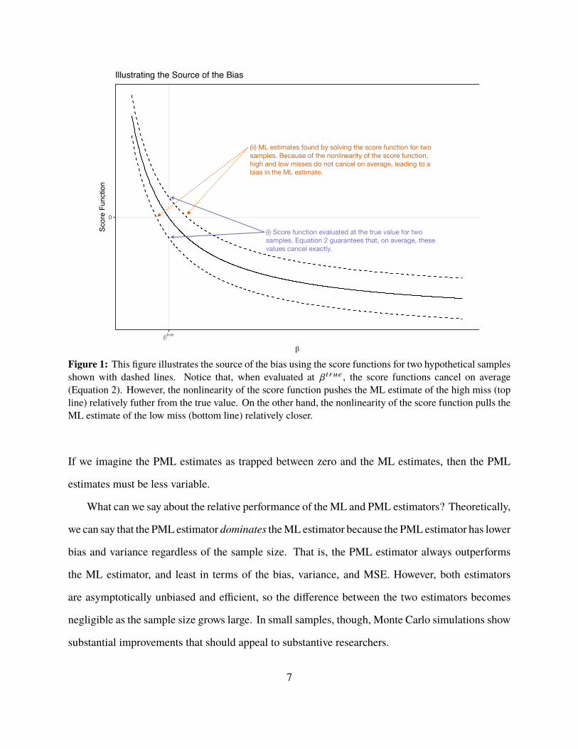
The intuition of the bias reduction is subtle. First, consider the source of the bias, illustrated

in Figure 1. Calculate the score function s as the gradient (or first-derivative) of the log-likelihood

with respect to β so that s(y, β) = ∇ log L(β |y). Note that solving s(y, β̂mle) = 0 is equivalent

to finding β̂mle that maximizes log L(β |y). Now recall that at the true parameter vector βtrue, the

expected value of the score function is zero so that E[s(y, βtrue)

]= 0 (Greene 2012, p. 517). By

7The penalized maximum likelihood estimates are easy to calculate in R using the logistf (Heinze et al. 2013) orbrglm (Kosmidis 2017a) packages and in Stata with the firthlogit (Coveney 2015) module. See the Section A andSection B of the Appendix, respectively, for examples.

5

the law of total probability, this implies that

E[s(y, βtrue) |s(y, βtrue) > 0

]= −E

[s(y, βtrue) |s(y, βtrue) < 0

], (2)

which is highlighted by (i) in Figure 1.

However, if the score function s is decreasing and curved in the area around βtruej so that

s′′j =∂2s(y, β)∂2 β j

> 0 (see Figure 1), then a high miss s(y, βtrue) > 0 (top dashed line in Figure 1)

implies an estimate well above the true value, so that β̂mle >> βtrue, and a low miss (bottom

dashed line in Figure 1) s(y, βtrue) < 0 implies an estimate only slightly below the true value, so

that β̂mle < βtrue. In effect, the curved (convex) score function pulls low misses closer the true

value and pushes high misses even further from the true value. This dynamic, which is highlighted

by (ii) in Figure 1, implies that low misses and high misses do not cancel and that the ML estimate

is too large on average. A similar logic applies for s′′j < 0. Therefore, due to the curvature in the

score function s, the high and low misses of β̂mle do not cancel out, so that E( β̂mlej ) > βtrue

j when

s′′j > 0 and E( β̂mle) < βtruej when s′′j < 0. Cox and Snell (1968, pp. 251-252) derive a formal

statement of this bias of order n−1, which we denote as biasn−1 (βtrue).

Now consider the bias reduction strategy. At first glance, one may simply decide to subtract

biasn−1 (βtrue) from the estimate β̂mle. However, note that the bias depends on the true parameter.

Because researchers do not know the true parameter, this is not the most effective strategy.8

However, Firth (1993) suggests modifying the score function, so that s∗(y, β) = s(y, β) − γ(β),

where γ shifts the score function upward or downward. Firth (1993) shows that one good choice

of γ takes γ j =12 trace

[I−1

(∂I∂ β j

)]= ∂

∂ β j

(log |I (β) |

). Integrating, we can see that solving

s∗(y, β̂pmle) = 0 is equivalent to finding β̂pmle that maximizes log L∗(β |y) with respect to β.

The intuition of the variance reduction is straightforward. Because PML shrinks the ML

estimates toward zero, the PML estimates must have a smaller variance than the ML estimates.

8However, Anderson and Richardson (1979) explore the option of correcting the bias by using β̂mle−biasn−1 ( β̂mle ).See Kosmidis (2014, esp. p. 190) for further discussion.

6

0

βtrue

β

Scor

e Fu

nctio

n

Illustrating the Source of the Bias

(i) Score function evaluated at the true value for two samples. Equation 2 guarantees that, on average, these values cancel exactly.

(ii) ML estimates found by solving the score function for two samples. Because of the nonlinearity of the score function, high and low misses do not cancel on average, leading to a bias in the ML estimate.

Figure 1: This figure illustrates the source of the bias using the score functions for two hypothetical samplesshown with dashed lines. Notice that, when evaluated at βtrue , the score functions cancel on average(Equation 2). However, the nonlinearity of the score function pushes the ML estimate of the high miss (topline) relatively futher from the true value. On the other hand, the nonlinearity of the score function pulls theML estimate of the low miss (bottom line) relatively closer.

If we imagine the PML estimates as trapped between zero and the ML estimates, then the PML

estimates must be less variable.

What can we say about the relative performance of the ML and PML estimators? Theoretically,

we can say that the PMLestimator dominates theML estimator because the PMLestimator has lower

bias and variance regardless of the sample size. That is, the PML estimator always outperforms

the ML estimator, and least in terms of the bias, variance, and MSE. However, both estimators

are asymptotically unbiased and efficient, so the difference between the two estimators becomes

negligible as the sample size grows large. In small samples, though, Monte Carlo simulations show

substantial improvements that should appeal to substantive researchers.

7

The Big Improvements from an Easy Solution

To show that the size of reductions in bias, variance, and MSE should draw the attention of

substantive researchers, we conduct aMonte Carlo simulation comparing the sampling distributions

of the ML and PML estimates. These simulations demonstrate three features of the ML and PML

estimators:

1. In small samples, the ML estimator exhibits a large bias. The PML estimator is nearly

unbiased, regardless of sample size.

2. In small samples, the variance of the ML estimator is much larger than the variance of the

PML estimator.

3. The increased bias and variance of the ML estimator implies that the PML estimator also has

a smaller MSE. Importantly, though, the variance makes a much greater contribution to the

MSE than the bias.

In our simulation, the true data generating process corresponds to Pr(yi = 1) = 11+e−Xi β

, where

i ∈ 1, 2, ..., n and X β = βcons + 0.5x1 +∑k

j=2 0.2x j , and we focus on the coefficient for x1 as the

coefficient of interest. We draw each fixed x j independently from a normal distribution with mean

of zero and standard deviation of one and vary the sample size N from 30 to 210, the number of

explanatory variables k from 3 to 6 to 9, and the the intercept βcons from -1 to -0.5 to 0 (which, in

turn, varies the proportion of events Pcons from about 0.28 to 0.38 to 0.50).9

Each parameter in our simulation varies the amount of information in the data set. The

biostatistics literature uses the number of events per explanatory variable 1k∑

yi as a measure of the

information in the data set (e.g., Peduzzi et al. 1996 and Vittinghoff andMcCulloch 2007), and each

parameter of our simulation varies this quantity, where N×Pcons

k ≈ 1k∑

yi. For each combination

of the simulation parameters, we draw 50,000 data sets and use each data set to estimate the logit

9Creating a correlation among the x j ’s has the same effect as decreasing the sample size.

8

model coefficients usingML and PML. To avoid an unfair comparison, we exclude theML estimates

where separation occurs (Zorn 2005). We keep all the PML estimates. Replacing the ML estimates

with the PML estimates when separation occurs dampens the difference between the estimators and

keeping all the ML estimates exaggerates the differences. From these estimates, we compute the

percent bias and variance of the ML and PML estimators, as well as the MSE inflation of the ML

estimator compared to the PML estimator.

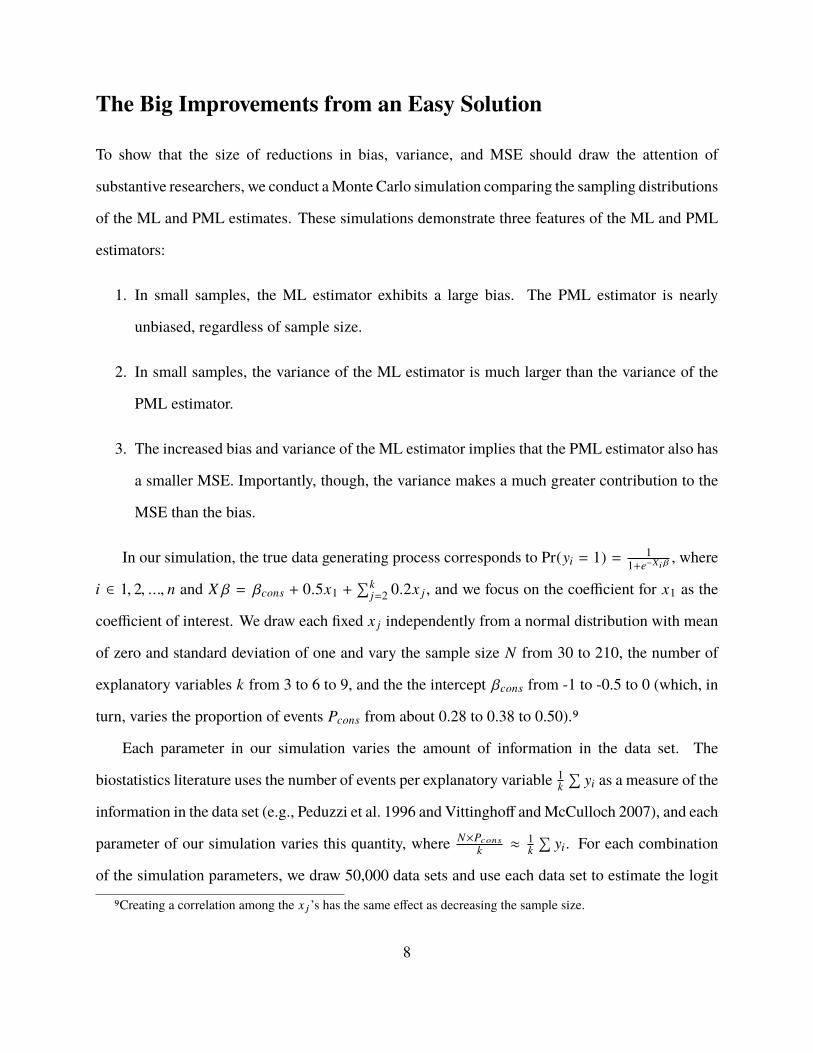
Bias

We calculate the percent bias = 100×(

E( β̂)βtrue − 1

)as the intercept βcons, the number of explanatory

variables k, and the sample size N vary. Figure 2 shows the results. The sample size varies

across the horizontal-axis of each plot and each panel shows a distinct combination of intercept and

number of variables in the model. Across the range of the parameters of our sample, the bias of the

ML estimate varies from about 69% (βcons = −1, k = 9, and N = 30) to around 3% (βcons = 0,

k = 3, and N = 210). The bias in the PML estimate, on the other hand, is much smaller. For the

worst-case scenario (βcons = −1, k = 9, and N = 30), the ML estimate has an upward bias of about

69%, while the PML estimate has an upward bias of only about 6%.10

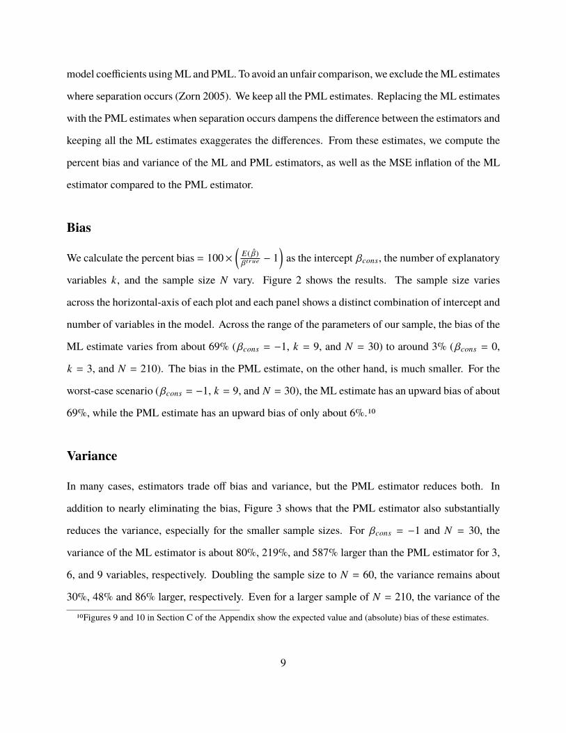
Variance

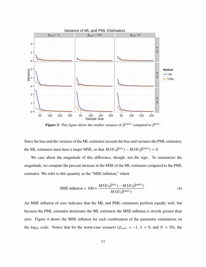
In many cases, estimators trade off bias and variance, but the PML estimator reduces both. In

addition to nearly eliminating the bias, Figure 3 shows that the PML estimator also substantially

reduces the variance, especially for the smaller sample sizes. For βcons = −1 and N = 30, the

variance of the ML estimator is about 80%, 219%, and 587% larger than the PML estimator for 3,

6, and 9 variables, respectively. Doubling the sample size to N = 60, the variance remains about

30%, 48% and 86% larger, respectively. Even for a larger sample of N = 210, the variance of the

10Figures 9 and 10 in Section C of the Appendix show the expected value and (absolute) bias of these estimates.

9

βcons = − 1 βcons = − 0.5 βcons = 0

0%

30%

60%

90%

0%

30%

60%

90%

0%

30%

60%

90%

k=

3k

=6

k=

9

50 100 150 200 50 100 150 200 50 100 150 200Sample Size

Per

cent

Bia

s

Method

ML

PML

Percent Bias of ML and PML Estimators

Figure 2: This figure shows the substantial bias of β̂mle and the near unbiasedness of β̂pmle .

ML estimator is about 6%, 10%, and 15% larger than the PML estimator.11

Mean-Squared Error

However, neither the bias nor the variance serves as a complete summary of the performance of

an estimator. The MSE, though, combines the bias and variance into an overall measure of the

accuracy, where

MSE( β̂) = E[( β̂ − βtrue)2]

= V ar ( β̂) + [Bias( β̂)]2. (3)

11Figure 11 in the Appendix shows the variance inflation = 100 ×(Var (β̂mle )Var (β̂pmle )

− 1).

10

βcons = − 1 βcons = − 0.5 βcons = 0

0

1

2

0

1

2

0

1

2

k=

3k

=6

k=

9

50 100 150 200 50 100 150 200 50 100 150 200Sample Size

Var

ianc

e Method

ML

PML

Variance of ML and PML Estimators

Figure 3: This figure shows the smaller variance of β̂pmle compared to β̂mle .

Since the bias and the variance of theML estimator exceeds the bias and variance the PML estimator,

the ML estimator must have a larger MSE, so that MSE( β̂mle) − MSE( β̂pmle) > 0.

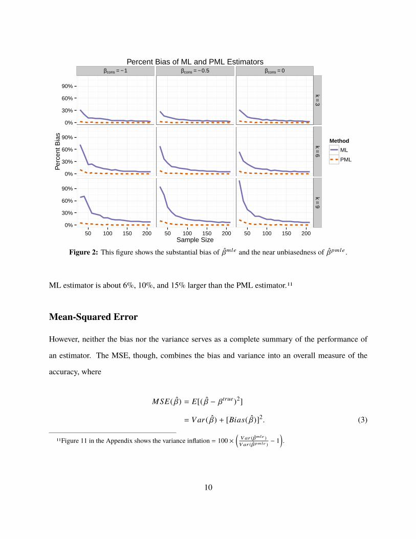
We care about the magnitude of this difference, though, not the sign. To summarize the

magnitude, we compute the percent increase in the MSE of the ML estimator compared to the PML

estimator. We refer to this quantity as the “MSE inflation,” where

MSE inflation = 100 ×MSE( β̂mle) − MSE( β̂pmle)

MSE( β̂pmle). (4)

An MSE inflation of zero indicates that the ML and PML estimators perform equally well, but

because the PML estimator dominates the ML estimator, the MSE inflation is strictly greater than

zero. Figure 4 shows the MSE inflation for each combination of the parameter simulations on

the log10 scale. Notice that for the worst-case scenario (βcons = −1, k = 9, and N = 30), the

11

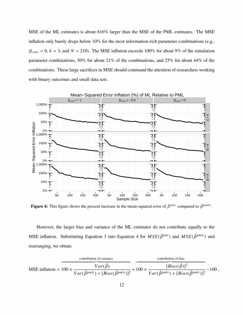
MSE of the ML estimates is about 616% larger than the MSE of the PML estimates. The MSE

inflation only barely drops below 10% for the most information-rich parameter combinations (e.g.,

βcons = 0, k = 3, and N = 210). The MSE inflation exceeds 100% for about 9% of the simulation

parameter combinations, 50% for about 21% of the combinations, and 25% for about 44% of the

combinations. These large sacrifices in MSE should command the attention of researchers working

with binary outcomes and small data sets.

βcons = − 1 βcons = − 0.5 βcons = 0

1%

10%

100%

1,000%

1%

10%

100%

1,000%

1%

10%

100%

1,000%

k=

3k

=6

k=

9

50 100 150 200 50 100 150 200 50 100 150 200Sample Size

Mea

n−S

quar

ed E

rror

Infla

tion

Mean−Squared Error Inflation (%) of ML Relative to PML

Figure 4: This figure shows the percent increase in the mean-squared error of β̂mle compared to β̂pmle .

However, the larger bias and variance of the ML estimator do not contribute equally to the

MSE inflation. Substituting Equation 3 into Equation 4 for MSE( β̂mle) and MSE( β̂pmle) and

rearranging, we obtain

MSE inflation =

contribution of variance︷ ︸︸ ︷100 ×

V ar ( β̂)V ar ( β̂pmle) + [Bias( β̂pmle)]2

+

contribution of bias︷ ︸︸ ︷100 ×

[Bias( β̂)]2

V ar ( β̂pmle) + [Bias( β̂pmle)]2−100 ,

12

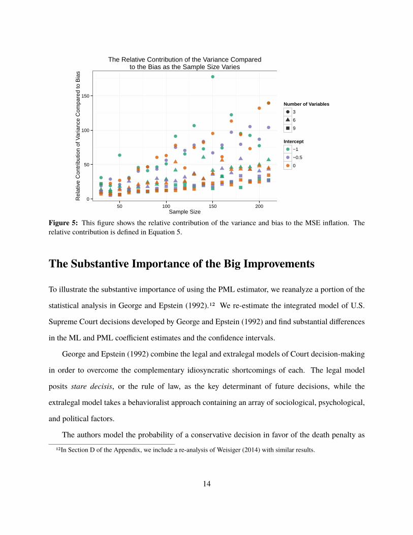
which additively separates the contribution of the bias and variance to the MSE inflation. If we

wanted, we could simply plug in the simulation estimates of the bias and variance of each estimator

to obtain the contribution of each. But notice that we can easily compare the relative contributions

of the bias and variance using the ratio

relative contribution of variance =contribution of variancecontribution of bias

. (5)

Figure 5 shows the relative contribution of the variance. Values less than one indicate that the bias

makes a greater contribution and values greater than one indicate that the variance makes a greater

contribution. In each case, the relative contribution of the variance is much larger than one. For

N = 30, the contribution of the variance is between 7 and 31 times larger than the contribution of

the bias. For N = 210, the contribution of the variance is between 27 and 140 times larger than the

contribution of the bias. In spite of the attention paid to the small sample bias in ML estimates of

logit model coefficients, the small sample variance is a more important problem to address, at least

in terms of the accuracy of the estimator. Fortunately, the PML estimator greatly reduces the bias

and variance, resulting in a much smaller MSE, especially for small samples.

These simulation results show that the bias, variance, and MSE of the ML estimates of logit

model coefficients are not trivial in small samples. Researchers cannot safely ignore these problems.

Fortunately, researchers can implement the PML estimator with little to no added effort and obtain

substantial improvements over the usual ML estimator. And these improvements are not limited

to Monte Carlo studies. In the example application that follows, we show that the PML estimator

leads to substantial reductions in the magnitude of the coefficient estimates and in the width of the

confidence intervals.

13

0

50

100

150

50 100 150 200Sample Size

Rel

ativ

e C

ontr

ibut

ion

of V

aria

nce

Com

pare

d to

Bia

s

Number of Variables

3

6

9

Intercept

−1

−0.5

0

The Relative Contribution of the Variance Comparedto the Bias as the Sample Size Varies

Figure 5: This figure shows the relative contribution of the variance and bias to the MSE inflation. Therelative contribution is defined in Equation 5.

The Substantive Importance of the Big Improvements

To illustrate the substantive importance of using the PML estimator, we reanalyze a portion of the

statistical analysis in George and Epstein (1992).12 We re-estimate the integrated model of U.S.

Supreme Court decisions developed by George and Epstein (1992) and find substantial differences

in the ML and PML coefficient estimates and the confidence intervals.

George and Epstein (1992) combine the legal and extralegal models of Court decision-making

in order to overcome the complementary idiosyncratic shortcomings of each. The legal model

posits stare decisis, or the rule of law, as the key determinant of future decisions, while the

extralegal model takes a behavioralist approach containing an array of sociological, psychological,

and political factors.

The authors model the probability of a conservative decision in favor of the death penalty as

12In Section D of the Appendix, we include a re-analysis of Weisiger (2014) with similar results.

14

a function of a variety of legal and extralegal factors. George and Epstein use a small sample of

64 Court decisions involving capital punishment from 1971 to 1988. The data set has only with

29 events (i.e., conservative decisions). They originally use the ML estimator and we reproduce

their estimates exactly. For comparison, we also estimate the model with the PML estimator that

we recommend. Figure 6 shows the coefficient estimates for each method. In all cases, the PML

estimate is smaller than the ML estimate. Each coefficient decreases by at least 25% with three

decreasing by more than 40%. Additionally, the PML estimator substantially reduces the width of

all the confidence intervals. Three of the 11 coefficients lose statistical significance.

●●

●●

●●

●●

●●

●●

●●

●●

●●

●●

●●

N = 64 (29 events)Death−Qualified Jury

Capital Punishment Proportional to Offense

Particularizing Circumstances

Aggravating Factors

State Psychiatric Examination

Conservative Political Environment

Court Change

State Appellant

Inexperienced Defense Counsel

Repeat Player State

Amicus Brief from Solicitor General

0.0 2.5 5.0 7.5Logit Model Coefficients and 90% Confidence Intervals

(Intercept Not Shown)

Method

●

●

ML

PML

Logit Model Explaining Conservative Court Decisions

Figure 6: This figure shows the coefficients for a logit modelmodel estimatingU.S. SupremeCourt Decisionsby both ML and PML.

Because we do not know the true model, we cannot know which of these sets of coefficients

is better. However, we can use out-of-sample prediction to help adjudicate between these two

methods. We use leave-one-out cross-validation and summarize the prediction errors using Brier

and log scores, for which smaller values indicate better predictive ability.13 The ML estimates

13The Brier score is calculated as∑n

i=1(yi − pi )2, where i indexes the observations, yi ∈ {0, 1} represents the actual

15

produce a Brier score of 0.17, and the PML estimates lower the Brier score by 8% to 0.16.

Similarly, the ML estimates produce a log score of 0.89, while the PML estimates lower the log

score by 41% to 0.53. The PML estimates outperform the ML estimates for both approaches to

scoring, and this provides good evidence that the PML estimates better capture the data generating

process.

Because we estimate a logit model, we are likely more interested in the functions of the

coefficients rather than the coefficients themselves (King, Tomz, and Wittenberg 2000). For an

example, we take George and Epstein’s integrated model of Court decisions and calculate a first

difference and risk ratio as the repeat-player status of the state varies, setting all other explanatory

variables at their sample medians. George and Epstein hypothesize that repeat players have greater

expertise and are more likely to win the case. Figure 7 shows the estimates of the quantities of

interest.

The PML estimator pools the estimated probabilities toward one-half. When the state is not

a repeat player, the PML estimates suggest a 17% chance of a conservative decision while ML

estimates suggest only a 6% chance. However, when the state is a repeat player, the PML estimates

suggest that the Court has a 53% chance of a conservative decision compared to the 60% chance

suggested by ML. Thus, PML also provides smaller effect sizes for both the first difference and the

risk ratio. PML decreases the estimated first difference by 17% from 0.63 to 0.52 and the risk ratio

by 67% from 12.3 to 4.0.

This example application clearly highlights the differences between the ML and PML estima-

tors. The PML estimator shrinks the coefficient estimates and confidence intervals substantially.

Theoretically, we know that these estimates have a smaller bias, variance, and MSE. Practically,

though, this shrinkage manifests in smaller coefficient estimates, smaller confidence intervals, and

outcome, and pi ∈ (0, 1) represents the estimated probability that yi = 1. The log score as −∑n

i=1 log(ri ), whereri = yipi + (1− yi )(1− pi ). Notice that because we are logging ri ∈ [0, 1],

∑ni=1 log(ri ) is always negative and smaller

(i.e., more negative) values indicate worse fit. Notice that we use the negative of∑n

i=1 log(ri ), so that, like the Brierscore, larger values indicate a worse fit.

16

●

●

●

●

0.68

0.06

0.69

0.17

0.0

0.2

0.4

0.6

Not a Repeat Player Repeat Player

Pro

babi

lity

Method

●

●

ML

PML

Probability of a Conservative Decision

●

●

0.63

0.52

PML estimate is 17% lowerthan ML estimate.

ML

PML

0.2 0.4 0.6 0.8First Difference

Met

hod

First Difference

●

●

12.3

4

PML estimate is 67% lowerthan ML estimate.

ML

PML

1 10 100Risk Ratio (Log Scale)

Met

hod

Risk Ratio

Figure 7: This figure shows the quantities of interest for the effect of the solicitor general filing a briefamicus curiae on the probability of a decision in favor of capital punishment.

better out-of-sample predictions. And these improvements come at almost no cost to researchers.

The PML estimator is nearly trivial to implement but dominates the ML estimator–the PML esti-

mator always has lower bias, lower variance, and lower MSE.

Recommendations to Substantive Researchers

Throughout this paper, we emphasize one key point–when using small samples to estimate logit

and probit models, the PML estimator offers a substantial improvement over the usual maximum

likelihood estimator. But what actions should substantive researchers take in response to our

17

methodological point? In particular, at what sample sizes should researchers consider switching

from the ML estimator to the PML estimator?

Concrete Advice About Sample Sizes

Prior research suggests two rules of thumb about sample sizes. First, Peduzzi et al. (1996)

recommend about 10 events per explanatory variable, though Vittinghoff and McCulloch (2007)

suggest relaxing this rule. Second, Long (1997, p. 54) suggests that “it is risky to use ML with

samples smaller than 100, while samples larger than 500 seem adequate.” In both of these cases, the

alternative to a logit or probit model seems to be no regression at all. Here though, we present the

PML estimator as an alternative, so we have room to make more conservative recommendations.

On the grounds that the PML estimator dominates the ML estimator, we might recommend

that researchers always use the PML estimator. But we do not want or expect researchers to

switch from the common and well-understood ML estimator to the PML estimator without a clear,

meaningful improvement in the estimates. While the PML estimator is theoretically superior, it

includes practical costs. Indeed, even though the R packages brglm (Kosmidis 2017a), brglm2

(Kosmidis 2017b), and logistf (Heinze and Ploner 2016) and the Stata module FIRTHLOGIT

(Coveney 2015) make fitting these models quick and easy, this approach might require researchers

to write custom software to compute quantities of interest. Further, the theory behind the approach

is less familiar to most researchers and their readers. Finally, these models are much more

computationally demanding. While the computational demands of a single PML fit are trivial,

this costs might become prohibitive for procedures requiring many fits, such as bootstrap or Monte

Carlo simulations. With these practical costs in mind, we use a Monte Carlo simulation to develop

rules of thumb that link the amount of information in the data set to the cost of using ML rather

than PML.

We measure the cost of using ML rather than PML as the MSE inflation defined in Equation 4:

the percent increase in the MSE when using ML rather than PML. The MSE inflation summarizes

18

the relative inaccuracy of the ML estimator compared to the PML estimator.

To measure the information in a data set, the biostatistics literature suggests using the number

of events per explanatory variable 1k∑

yi (e.g., Peduzzi et al. 1996 and Vittinghoff and McCulloch

2007). However, we modify this metric slightly and consider the minimum of the number of events

and the number of non-events. This modified measure, which we denote as ξ, has the attractive

property of being invariant to flipping the coding of events and non-events. Indeed, one could not

magically increase the information in a conflict data set by coding peace-years as ones and conflict-

years as zeros. With this in mind, we use a measure of information ξ that takes the minimum of

the events and non-events per explanatory variable, so that

ξ =1kmin

n∑i=1

yi,

n∑i=1

(1 − yi). (6)

The cost of usingML rather than PMLdecreases continuouslywith the amount of information in

the data set, but to make concrete suggestions, we break the costs into three categories: substantial,

noticeable, and negligible. We use the following cutoffs.

1. Negligible: If the MSE inflation probably falls below 3%, then we refer to the cost as

negligible.

2. Noticeable: If the MSE inflation of ML probably falls below 10%, but not probably below

3%, then we refer to the cost as noticeable.

3. Substantial: If the MSE inflation of ML might rise above 10%, then we refer then the cost as

substantial.

To develop our recommendations, we estimate theMSE inflation for awide range of hypothetical

analyses across which the true coefficients, the number of explanatory variables, and the sample

size varies.

To create each hypothetical analysis, we do the following:

19

1. Choose the number of covariates k randomly from a uniform distribution from 3 to 12.

2. Choose the sample size n randomly from a uniform distribution from 200 to 3,000.

3. Choose the intercept βcons randomly from a uniform distribution from -4 to 4.

4. Choose the slope coefficients β1, ..., βk randomly from a normal distribution with mean 0

and standard deviation 0.5.

5. Choose a covariance matrix Σ for the explanatory variables randomly using the method

developed by Joe (2006) such that the variances along the diagonal range from from 0.25 to

2.

6. Choose the explanatory variables x1, x2, ..., xk randomly from a multivariate normal distri-

bution with mean 0 and covariance matrix Σ.

7. If these choices produce a data set with less than 20% events or non-events, then we discard

this analysis.

Note that researchers should not apply our rules of thumb to rare events data (King and Zeng 2001),

because they are overly conservative. As the sample size increases, the MSE inflation drops, even

if ξ is held constant. By the design of our simulation study, our guidelines apply to events more

common than 20% and less common than 80%. However, researchers using rare events data should

view our recommendations as conservative; as the sample size increases, the MSE tends to shrink

relative to ξ.14

For each hypothetical analysis, we simulate 2,000 data sets and compute the MSE inflation of

theML estimator relative to the PML estimator using Equation 4. We then use quantile regression to

model the 90th percentile as a function of the information ξ in the data set. This quantile regression

allows us to estimate the amount of information that researchers need to before the MSE inflation

14A more complicated, but precise, set of rules might rely on sample size and ξ, but then they are no longer rules ofthumb and fail to provide simple guidelines.

20

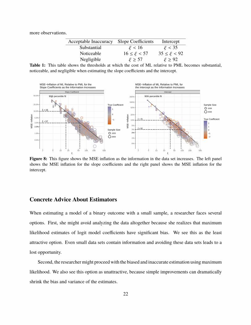
“probably” (i.e., about a 90% chance) falls below some threshold. We then calculate the thresholds

at which the MSE inflation probably falls below 10% and 3%. Table 1 shows the thresholds and

Figure 8 shows the MSE for each hypothetical analysis and the quantile regression fits.

Interestingly, ML requires more information to estimate the intercept βcons accurately relative

to PML than the slope coefficients β1, ..., βk (see King and Zeng 2001). Because of this, we

calculate the cutoffs separately for the intercept and slope coefficients.

If the researcher simply wants accurate estimates of the slope coefficients, then she risks

substantial costs when using ML with ξ ≤ 16 and noticeable costs when using ML with ξ ≤ 57. If

the researcher also wants an accurate estimate of the intercept, then she risks substantial costs when

using ML with ξ ≤ 35 and noticeable costs when using ML when ξ ≤ 92. Researchers should treat

these thresholds as rough rules of thumb–not strict guidelines. Indeed, the MSE inflation depends

on a complex interaction of many features of the analysis, including the number of covariates,

their distribution, the magnitude of their effects, the correlation among them, and the sample size.

However, these (rough) rules accomplish two goals. First, they provide researchers with a rough

idea of when the choice of estimator might matter. Second, they highlight that analysis with samples

typically considered “large enough” for ML might benefit from using PML instead.

Importantly, the cost of ML only becomes negligible for all model coefficients when ξ > 92–

this threshold diverges quite a bit from the prior rules of thumb. For simplicity, assume the

researcher wants to include eight explanatory variables in her model. In the best case scenario of

50% events, she should definitely use the PML estimator with fewer than 8×160.5 = 256 observations

and ideally use the PML estimator with fewer than 8×570.5 = 912 observations. But if she would

also like accurate estimates of the intercept, then these thresholds increase to 8×350.5 = 560 and

8×920.5 = 1, 472 observations. Many logit and probit models estimated using survey data have fewer

than 1,500 observations and these studies risk a noticeable cost by using the ML estimator rather

than the PML estimator. Further, these estimates assume 50% events. As the number of events

drifts toward 0% or 100% or the number of variables increases, then the researcher needs even

21

more observations.

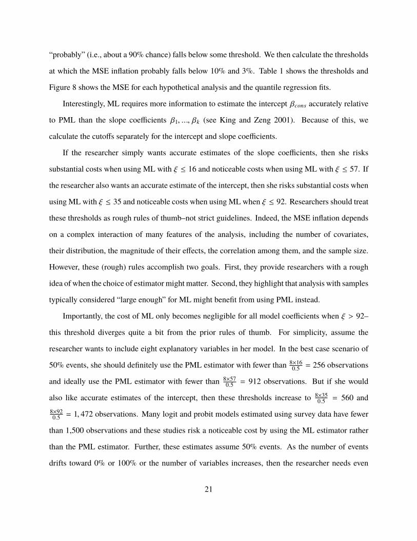
Acceptable Inaccuracy Slope Coefficients InterceptSubstantial ξ < 16 ξ < 35Noticeable 16 ≤ ξ < 57 35 ≤ ξ < 92Negligible ξ ≥ 57 ξ ≥ 92

Table 1: This table shows the thresholds at which the cost of ML relative to PML becomes substantial,noticeable, and negligible when estimating the slope coefficients and the intercept.

●●●●●●

●

●●●●

●●●●●●●●●

●●●●●●●●●●●●

●●●●

●●

●

●●●●●●●

●●●

●●●●

●

●●●

●●

●●

●

●

●

●●

●●●●●

●

●

●●

●

●●●●●● ●

●

●●●●

●●●●●●●

●●●●●●●●●●●

●

●●●●●●●●●

●●●●●●

●●●●●●●●●

●●●●●●●●●●●●●●●●●

●●●●●●●●●●●●

●●●●●

●

●●●●●●●●●

●

●●●●●●

●●●●●●●●●●●●●●

●●●●●●●●●●●

●

●●●●●●●●●●●●●

●●

●

●●●●●●●●

●●●●●

●●●●●●●●●

●●●●●●●●

●●●●●●●● ●●●●

●●●●●●●●●●●●●●●●●●●●●●●

●●●●●●●●●

●●●●●●●

●●●●●●●●●●

●●●

●●●●●

●

●

●

●●●●●●●●●●●●●●● ●

●●●●●●●●●●

●●●●●●●●●●●

●

●●●●

●●●

●

●

●●●●●●●

●●●●●

●

●●●

●●●●●●●●●●

●●●●

●●●●●●●●●

●

●

●●●

●●●●

●●●

●●●●●●

●●●

●●●●

●

●

●●●●●●●●●●●

●●●●●●● ●●●●●●●●●●●●

●●●●●●●●●●●

●●

●

●●●●●

●●●●●●●●

●●●

●●●●●●●●

●●●●●●●●

●●●●●●●●●●●●●

●

●●●●

●

●●●

●●●●

●●●

●●●●●●●

●

●

●●

●●●●●●●

●

●●●●●●

●●●●

●

●●●●●●●●●

●

●●●●

●

●●

●●●●●

●●●●●●

●●●●●●●●●●

●

●●●●●●●●●●

●●●●●●●●●●●

●●●

●●●●●

●●●●●●●●●●●●●●●●●●●●●●●●●●●●●●●●●● ●

●●●

●●●●●●●

●

●●●●●●●●

●●●●●●●

●●●●●

●●●●●●●●

●

●●●●

●

●●●●●●●●

●●●●●●●●●●●

●●●●●

●●●●●●●●●●

●●●

●●●●●●●●●●

●●●●●●●●●●●●

●●●●●●●●●

●●●●●●●●

●●●

●●●

●●

●●●●●●●●●●●

●●●●●●●●●●●

●●●●

●●●●●

●●●

●●●●●

●●

●

●●●●●●●

●●●●●●●●●●●●●●●

●●●●●●●●●●●●

●

●●

●

●●●

●●●●

●●●●●●●

●●●●●

●●●●

●●●●●

●●●●●●●●●●●●●

●

●●

●●●

●●●●●●●

●

●●

●

●●●

●●●●●

●

●●●●●●●●●●●●●●●●

●●●●●●●●●

●●●●●●●●●

●

●●●●

●●●●●●●

●●●●●●●

●●●●

●

●●●

●

●

●

●●●●●●●●●●●●

●●●●●●●●●●

●

●●●

●●●●●●●●●

●●●●●●

●

●

●●●●●●●●●

●●●

●●●●●●●●●●●

●●●●●●●●● ●●●●●●

●●●●●●●●●●●

●●●●●●●●●●

●●●●●

●●●●●●●●●●●●●

●●●●●●●●●●●● ●●●●●●●●●●

●

●

●●●●●●●●●

●●●●●●●●●●

●●●●●●●●●●●

●●●●●●●●●●

●●●●●●●●●●●●

●●●●●●●●●●●

●●●●●●●

●●●●●●

●●●●

●●●●●●●●●●●

●

●

●

●●●●

●

●

●

●

●●●●●●●

●●●●●

●●●●●●●

●●●●●●●●●●●●●●●●●

●

●●

●●●●●●●

●●●●●●●●●●●●

●●●●●●●●●●●●●

●●●●●●

●●●

●

●

●●●●●

●●●●

●●●●● ●●●●●●●●

●

●●

●●●●●

●●●●●

●●

●●●●

●●●●●

●

●●

●●●●●●●●●● ●●●●●●●●●

●

●

●●●●●

●

●●●●●●●●●●●●●●

●●●●●

●

●

●

●●●●●●●●●●●

●●●

●●●●●●●●●

●●●●●●●●●●●●

●●●●●●

●●●●●●●●

●●●●●●●

●●●●●●●●●●●●●●●●●●●●●

●●●●●●●●●●

●●●●●●●●●●●●

●●●●●●●●●●●

●●●●●●●●

●●●●●●●●●●●●

●●●●

●

●●

●●●●●●●

●●●●●●●●●●●

●●●●●●●

●●●

●

●●●●

●●●●●●●●●

●●●●●

●●●●●●●

●●●●●●●●●●

●●●●●

●●●

●●

●●●●

●●●

●●●●●

●

●●●●●●

●●●

●●●●●

●●●●●●●●●●

●●●●●●●●●●

●●●●●●●●

●●●●●●

●●●●●●●●●●●

●●●●●●●

●

●●●●●●●

●●

●●●●●●●●

●●●●●

●●●●●●●●●●

●●●

●●●

●●●

●●●

●

●●●●

ξ = 57

ξ = 16

90th percentile fit

Slope Coefficient

2 5 10 20 50 100 200 500

0.5%

1.0%

2.0%2.0%

3.0%

5.0%

10.0%

20.0%

50.0%

ξ

MS

E−

Infla

tion

−1

0

1

True Coefficient

Sample Size

●

●

1000

2000

MSE−Inflation of ML Relative to PML for theSlope Coefficients as the Information Increases

●

●

●

●●

●●

●

●

●

●●

●

●

●

●

●

●

●

●●

●

●

●

●

●

●

●

●

●

●● ●

●

●●

● ●

●

●●

●

●

●

●

●

●

●●

●●

●

●

●

●

●●

●

●

●

●

●

●

●

●

●

●●

●●

●

●

●

● ●●

●

●

●

●

●

●

●●●

●

●

●

●

●

●●

●

●●●

●

●

●

●

●

●

●

●

●●

●

●

●

●●●

●

●

●

●

●

●

●

●

●

●

●

●

●

●●●

●

●

●

●

●

●

●

●

●●

●

●

●

●

●●

●

●

●

●

●

●●

●

●●

●●●

●

●

●

●●

●

●●

●

●

●

●

●

●

●

●●

●

●

●

●

●

●

●●●●●

●

●●

●●●

●

●

●●

●●

●●●●

●

●

●

●

●

●

●

●

●

●

●

●●

●

●

● ●●

●

● ●●

●●

●

●

●ξ = 92

ξ = 35

90th percentile fit

Intercept

2 5 10 20 50 100 200 500

0%

1%

2%2%

3%

5%

10%

20%

50%

100%

200%

ξ

MS

E−

Infla

tion

Sample Size

●

●

1000

2000

−2

−1

0

1

2

True Coefficient

MSE−Inflation of ML Relative to PML forthe Intercept as the Information Increases

Figure 8: This figure shows the MSE inflation as the information in the data set increases. The left panelshows the MSE inflation for the slope coefficients and the right panel shows the MSE inflation for theintercept.

Concrete Advice About Estimators

When estimating a model of a binary outcome with a small sample, a researcher faces several

options. First, she might avoid analyzing the data altogether because she realizes that maximum

likelihood estimates of logit model coefficients have significant bias. We see this as the least

attractive option. Even small data sets contain information and avoiding these data sets leads to a

lost opportunity.

Second, the researchermight proceedwith the biased and inaccurate estimation usingmaximum

likelihood. We also see this option as unattractive, because simple improvements can dramatically

shrink the bias and variance of the estimates.

22

Third, the researcher might use least squares to estimate a linear probability model (LPM). If

the probability of an event is a linear function of the explanatory variables, then this approach is

reasonable, as long as the researcher takes steps to correct the standard errors. However, in most

cases, using an “S”-shaped inverse-link function (i.e., logit or probit) makes the most theoretical

sense, so that marginal effects shrink toward zero as the probability of an event approaches zero or

one (e.g., Berry, DeMeritt, and Esarey 2010 and Long 1997, pp. 34-47). Long (1997, p. 40) writes:

“In my opinion, the most serious problem with the LPM is its functional form.” Additionally, the

LPM sometimes produces nonsense probabilities that fall outside the [0, 1] interval and nonsense

risk ratios that fall below zero. If the researcher is willing to accept these nonsense quantities and

assume that the functional form is linear, then the LPM offers a reasonable choice. However, we

agree with Long (1997) that without evidence to the contrary, the logit or probit model offers a

more plausible functional form.

Fourth, the researchermight use a bootstrap procedure (Efron 1979) to correct the bias of theML

estimates. While in general the bootstrap presents a risk of inflating the variance when correcting

the bias (Efron and Tibshirani 1993, esp. pp. 138-139), simulations suggest that the procedure

works comparably to PML in some cases for estimating logit model coefficients. However, the

bias-corrected bootstrap has a major disadvantage. When a subset of the bootstrapped data sets have

separation (Zorn 2005), which is highly likely with small data sets, then the bootstrap procedure

produces unreliable estimates. In this scenario, the bias and variance can be much larger than even

the ML estimates and sometimes wildly incorrect. Given the extra complexity of the bootstrap

procedure and the risk of unreliable estimates, the bias-corrected bootstrap is not particularly

attractive.

Finally, the researcher might simply use penalized maximum likelihood, which allows the

theoretically-appealing “S”-shaped functional form and fast estimation while greatly reducing the

bias and variance. Indeed, the penalized maximum likelihood estimates always have a smaller bias

and variance than the maximum likelihood estimates. These substantial improvements come at

23

almost no cost to the researcher in learning new concepts or software beyond maximum likelihood

and simple commands in R and/or Stata.15 We see this as the most attractive option. Whenever

researchers have concerns about bias and variance due to a small sample, a simple switch to a

penalized maximum likelihood estimator can quickly ameliorate any concerns with little to no

added difficulty for researchers or their readers.

ReferencesAnderson, J. A., and S. C. Richardson. 1979. “Logistic Discrimination and Bias Correction inMaximum Likelihood Estimation.” Technometrics 21(1):71–78.

Barrilleaux, Charles, and Carlisle Rainey. 2014. “The Politics of Need: Examining Governors’Decisions to Oppose the ‘Obamacare’ Medicaid Expansion.” State Politics and Policy Quarterly14(4):437–460.

Bell, Mark S., and Nicholas L. Miller. 2015. “Questioning the Effect of Nuclear Weapons onConflict.” Journal of Conflict Resolution 59(1):74–92.

Berry, William D., Jacqueline H. R. DeMeritt, and Justin Esarey. 2010. “Testing for Interaction inBinary Logit and Probit Models: Is a Product Term Essential.” American Journal of PoliticalScience 54(1):105–119.

Betz, Timm. 2015a. “Domestic Politics and the Initiation of International Disputes.” Workingpaper. Copy at http://people.tamu.edu/∼timm.betz/Betz-2014-Disputes.pdf.

Betz, Timm. 2015b. Trading Interests: Domestic Institutions, International Negotiations, andthe Politics of Trade. Chapter 3: Political Rhetoric and Trade. PhD Disseration University ofMichigan, Ann Arbor.

Casella, George, and Roger L. Berger. 2002. Statistical Inference. 2nd ed. Pacific Grove, CA:Duxbury.

Chacha, Mwita, and Jonathan Powell. 2017. “Economic interdependence and post-coup democra-tization.” Democratization 24(5):819–838.

Copas, John B. 1988. “Binary Regression Models for Contaminated Data.” Journal of the RoyalStatistical Society, Series B 50(2):225–265.

15Appendices A and B offer a quick overview of computing penalized maximum likelihood estimates in R and Stata,respectively.

24

Coveney, Joseph. 2015. “FIRTHLOGIT: Stata module to calculate bias reduction in logisticregressio.” Stata module.

Cox, D. R., and E. J. Snell. 1968. “A General Definition of Residuals.” Journal of the RoyalStatistical Society, Series B 30(2):248–275.

DeGroot, M. H., and M. J. Schervish. 2012. Probability and Statistics. 4th edition ed. Boston,MA: Wiley.

Efron, Bradley. 1979. “BootstrapMethods: Another Look at the Jackknife.” The Annals of Statistics7(1):1–26.

Efron, Bradley, and Robert J. Tibshirani. 1993. An Introduction to the Bootstrap. New York:Chapman and Hall.

Firth, David. 1993. “Bias Reduction of Maximum Likelihood Estimates.” Biometrika 80(1):27–38.

Gelman, Andrew. 2008. “Scaling Regression Inputs by Dividing by Two Standard Deviations.”Statistics in Medicine 27(15):2865–2873.

George, Tracey E., and Lee Epstein. 1992. “On the Nature of Supreme Court Decision Making.”American Political Science Review 86(2):323–337.

Greene, William H. 2012. Econometric Analysis. 7th ed. Upper Saddle River, New Jersey: PrenticeHall.

Hastie, Trevor, Robert Tibshirani, and JeromeFriedman. 2013. TheElements of Statistical Learning.Springer Series in Statistics second ed. New York: Springer.

Heinze, Georg, and Meinhard Ploner. 2016. logistf: Firth’s Bias-Reduced Logistic Regression.

Heinze, Georg, Meinhard Ploner, Daniela Dunkler, and Harry Southworth. 2013. logistf: Firth’sbias reduced logistic regression.

Jeffreys, H. 1946. “An Invariant Form of the Prior Probability in Estimation Problems.”Proceedingsof the Royal Society of London, Series A 186(1007):453–461.

Joe, Harry. 2006. “Generating Random Correlation Matrices Based on Partial Correlations.”Journal of Multivariate Analysis 97(10):2177–2189.

Kaplow, Jeffrey M., and Erik Gartzke. 2015. “Knowing Unknows: The Effect of Uncertainty inInterstate Conflict.” Working paper. Copy at http://dl.jkaplow.net/uncertainty.pdf.

King, Gary. 1998. Unifying Political Methodology: The Likelihood Theory of Statistical Inference.Ann Arbor: Michigan University Press.

King, Gary, and Langche Zeng. 2001. “Logistic Regression in Rare Events Data.” Political Analysis9(2):137–163.

25

King, Gary, Michael Tomz, and JasonWittenberg. 2000. “Making the Most of Statistical Analyses:Improving Interpretation and Presentation.” American Journal of Political Science 44(2):341–355.

Kosmidis, Ioannis. 2007. Bias Reduction in Exponential Family NonlinearModels PhDDisserationUniversity of Warwick.

Kosmidis, Ioannis. 2014. “Bias in Parametric Estimation: Reduction and Useful Side-Effects.”WIREs Computational Statistics 6(3):185–196.

Kosmidis, Ioannis. 2017a. brglm: Bias reduction in binary-response Generalized Linear Models.

Kosmidis, Ioannis. 2017b. brglm2: Bias reduction in generalized linear models.

Kosmidis, Ioannis, and David Firth. 2009. “Bias Reduction in Exponential Family NonlinearModels.” Biometrika 96(4):793–804.

Krueger, James S., andMichael S. Lewis-Beck. 2008. “Is OLSDead?” The Political Methodologist15(2):2–4.

Leeman, Lucas, and IsabellaMares. 2014. “The Adoption of Proportional Representation.” Journalof Politics 76(2):461–478.

Leonard, Thomas, and John S. J. Hsu. 1999. Bayesian Methods. Cambridge Series in Statisticaland Probabilistic Mathematics Cambridge: Cambridge University Press.

Long, J. Scott. 1997. Regression Models for Categorical and Limited Dependent Variables.Advanced Quantitative Techniques in the Social Sciences Thousand Oaks, CA: Sage.

McCullagh, Peter, and John A. Nelder. 1989. Generalized Linear Models. Second ed. Boca Raton,FL: Chapman and Hall.

Peduzzi, Peter, John Concato, Elizabeth Kemper, Theodore RHolford, andAlvan R Feinstein. 1996.“A Simulation Study of the Number of Events per Variable in Logistic Regression Analysis.”Journal of Clinical Epidemiology 49(12):1373–1379.

Poirier, Dale. 1994. “Jeffreys’ Prior for Logit Models.” Journal of Econometrics 63(2):327–339.

Rainey, Carlisle. 2016. “Dealing with Separation in Logistic RegressionModels.”Political Analysis24(3):339–355.

Vining, Jr., Richard L., Teena Wilhelm, and Jack D. Collens. 2015. “A Market-Based Model ofState Supreme Court News: Lessons from Captial Cases.” State Politics and Policy Quarterly15(1):3–23.

Vittinghoff, Eric, and Charles E. McCulloch. 2007. “Relaxing the Rule of Ten Events per Variablein Logistic and Cox Regression.” American Journal of Epidemiology 165(6):710–718.

26

Weisiger, Alex. 2014. “Victory Without Peace: Conquest, Insurgency, and War Termination.”Conflict Management and Peace Science 31(4):357–382.

Wooldridge, Jeffrey M. 2002. Econometric Analysis of Cross Section and Panel Data. Cambridge:MIT Press.

Zorn, Christopher. 2005. “A Solution to Separation in Binary Response Models.” Political Analysis13(2):157–170.

27

AppendixEstimating Logit Models with Small Samples

A PML Estimation in RThis example code is available at [redacted].

# load data from weblibrary(readr) # for read_csv()weisiger <- read_csv([redacted])

# quick look at datalibrary(dplyr) # for glimpse()glimpse(weisiger)

# model formulaf <- resist ~ polity_conq + lndist + terrain +soldperterr + gdppc2 + coord

# ----------------------------- ## pmle with the logistf package ## ----------------------------- #

# estimate logit model with pmlelibrary(logistf) # for logistf()m1 <- logistf(f, data = weisiger)

# see coefficient estimates, confidence intervals, p-values, etc.summary(m1)

# logistf does **NOT** work with texreg packagelibrary(texreg)screenreg(m1)

# see help file for morehelp(logistf)

# --------------------------- ## pmle with the brglm package ## --------------------------- #

# estimate logit model with pmlelibrary(brglm) # for brglm()m2 <- brglm(f, family = binomial, data = weisiger)

# see coefficient estimates, standard errors, p-values, etc.summary(m2)

28

# brglm works with texreg packagescreenreg(m2)

# see help file for morehelp(brglm)

B PML Estimation in StataThis example code is available at [redacted].The example data used is available at [redacted].

* set working directory and load data* data can be found at [redacted]cd "your working directory"insheet using "ge.csv", clear

* install firthlogitssc install firthlogit

* estimate logit model with pmle* see coefficient values, standard errors, p-values, etc.firthlogit court dq cr pc ag sp pe cc ap dc st sg

* see help file for morehelp firthlogit

29

C Additional Simulation Results

C.1 Expected Value

βcons = − 1 βcons = − 0.5 βcons = 0

0.5

0.6

0.7

0.8

0.9

1.0

0.5

0.6

0.7

0.8

0.9

1.0

0.5

0.6

0.7

0.8

0.9

1.0

k=

3k

=6

k=

9

50 100 150 200 50 100 150 200 50 100 150 200Sample Size

Exp

ecte

d V

alue

Method

ML

PML

Expected Value of ML and PML Estimators

Figure 9: This figure shows the expected value of β̂mle and β̂pmle . The true value is β = 0.5.

30

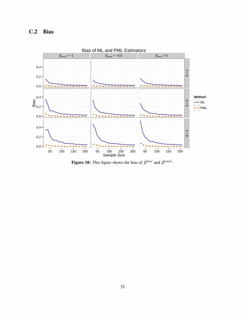
C.2 Bias

βcons = − 1 βcons = − 0.5 βcons = 0

0.0

0.2

0.4

0.0

0.2

0.4

0.0

0.2

0.4

k=

3k

=6

k=

9

50 100 150 200 50 100 150 200 50 100 150 200Sample Size

Bia

s

Method

ML

PML

Bias of ML and PML Estimators

Figure 10: This figure shows the bias of β̂mle and β̂pmle .

31

C.3 Variance Inflation

βcons = − 1 βcons = − 0.5 βcons = 0

0%

200%

400%

600%

0%

200%

400%

600%

0%

200%

400%

600%

k=

3k

=6

k=

9

50 100 150 200 50 100 150 200 50 100 150 200Sample Size

Var

ianc

e In

flatio

n

Variance Inflation (%) of ML Relative to PML

Figure 11: This figure shows the percent inflation in the variance of β̂mle compared to β̂pmle .

D Re-Analysis of Weisiger (2014)Weisiger describes how, after the official end of the war, violence sometimes continues in the formof guerrilla warfare. He argues that resistance is more likely when conditions are favorable forinsurgency, such as difficult terrain, a occupying force, or a pre-war leader remains at-large in thecountry.

Weisiger’s sample consists of 35 observations (with 14 insurgencies). We reanalyze Weisiger’sdata using a logit model to show the substantial difference between the biased, high-varianceML estimates and the nearly unbiased, low-variance PML estimates.16 Prior to estimation, we

16Specifically, we reanalyze the Model 3 in Weisiger’s Table 2 (p. 14). In the original analysis, Weisiger uses alinear probability model. He writes that “I [Weisiger] make use of a linear probability model, which avoids problemswith separation but introduces the possibility of non-meaningful predicted probabilities outside the [0,1] range” (p.11). As he notes, predictions outside the [0, 1] interval pose a problem for interpreting the linear probability model.In these data for example, the linear probability model estimates a probability of 1.41 of insurgency in one case. Inanother, it estimates a probability of -0.22. Overall, 25% of the estimated probabilities based on the linear probabilitymodel are larger than one or less than zero. Of course, these results are nonsense. However, because of the well-knownsmall-sample bias, methodologists discourage researchers from using a logit model with small samples. The PMLapproach, though, solves the problem of bias as well as nonsense predictions.

32

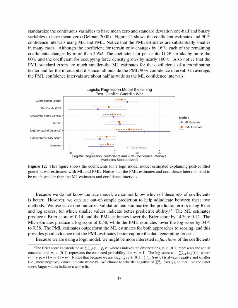
standardize the continuous variables to have mean zero and standard deviation one-half and binaryvariables to have mean zero (Gelman 2008). Figure 12 shows the coefficient estimates and 90%confidence intervals using ML and PML. Notice that the PML estimates are substantially smallerin many cases. Although the coefficient for terrain only changes by 16%, each of the remainingcoefficients changes by more than 45%! The coefficient for per capita GDP shrinks by more the60% and the coefficient for occupying force density grows by nearly 100%. Also notice that thePML standard errors are much smaller–the ML estimates for the coefficients of a coordinatingleader and for the intercapital distance fall outside the PML 90% confidence interval. On average,the PML confidence intervals are about half as wide as the ML confidence intervals.

●●

●●

●●

●●

●●

●●

●●

N = 35 (14 events)Intercept

Conqueror's Polity Score

log(Intercapital Distance)

Terrain

Occupying Force Density

Per Capita GDP

Coordinating Leader

−20 −10 0 10 20Logistic Regression Coefficients and 90% Confidence Intervals

(Variables Standardized)

Method

●

●

ML Estimate

PML Estimate

Logistic Regression Model ExplainingPost−Conflict Guerrilla War

Figure 12: This figure shows the coefficients for a logit model model estimated explaining post-conflictguerrilla war estimated with ML and PML. Notice that the PML estimates and confidence intervals tend tobe much smaller than the ML estimates and confidence intervals.

Because we do not know the true model, we cannot know which of these sets of coefficientsis better. However, we can use out-of-sample prediction to help adjudicate between these twomethods. We use leave-one-out cross-validation and summarize the prediction errors using Brierand log scores, for which smaller values indicate better predictive ability.17 The ML estimatesproduce a Brier score of 0.14, and the PML estimates lower the Brier score by 14% to 0.12. TheML estimates produce a log score of 0.58, while the PML estimates lower the log score by 34%to 0.38. The PML estimates outperform the ML estimates for both approaches to scoring, and thisprovides good evidence that the PML estimates better capture the data generating process.

Because we are using a logit model, we might be more interested in functions of the coefficients

17The Brier score is calculated as∑n

i=1(yi − pi )2, where i indexes the observations, yi ∈ {0, 1} represents the actualoutcome, and pi ∈ (0, 1) represents the estimated probability that yi = 1. The log score as −

∑ni=1 log(ri ), where

ri = yipi + (1− yi )(1− pi ). Notice that because we are logging ri ∈ [0, 1],∑n

i=1 log(ri ) is always negative and smaller(i.e., more negative) values indicate worse fit. We choose to take the negative of

∑ni=1 log(ri ), so that, like the Brier

score, larger values indicate a worse fit.

33

than in the coefficients themselves. For an example, we focus on Weisiger’s hypothesis that therewill be a greater chance of resistance when the pre-conflict political leader remains at large in theconquered country. Setting all other explanatory variables at their sample medians, we calculatedthe predicted probabilities, the first difference, and the risk ratio for the probability of a post-conflictguerrilla war as countries gain a coordinating leader. Figure 13 shows the estimates of the quantitiesof interest.

●

●

●

●

0.99

0.23

0.89

0.28

0.00

0.25

0.50

0.75

1.00

No Coordinating Leader Coordinating Leader

Pro

babi

lity

Method

●

●

ML

PML

Probability of a Post−Conflict Guerrilla War

●

●

0.75

0.61

PML estimate is 19% lowerthan ML estimate.

ML

PML

0.25 0.50 0.75First Difference

Met

hod

First Difference

●

●

4.2

3.2

PML estimate is 24% lowerthan ML estimate.

ML

PML

5 10 15Risk Ratio

Met

hod

Risk Ratio

Figure 13: This figure shows the quantities of interest for the effect of a coordinating leader on the probabilityof a post-conflict guerrilla war.

PML pools the estimated probabilities toward one-half, so that when a country lacks a coordi-nating leader, ML suggests a 23% chance of rebellion while PML suggests a 28% chance. On theother hand, when country does have a coordinating leader, ML suggests a 99% chance of rebellion,but PML lowers this to 89%. Accordingly, PML suggests smaller effect sizes, whether using a firstdifference or risk ratio. PML shrinks the estimated first difference by 19% from 0.75 to 0.61 andthe risk ratio by 24% from 4.2 to 3.2.

34