the probit & logit models - departamento de...

The Random Utility ModelThe Probit & Logit Models

Estimation & InferenceProbit & Logit Estimation in Stata

Summary

The Probit & Logit Models

Econometrics II

Ricardo Mora

Department of Economics

Universidad Carlos III de Madrid

Máster Universitario en Desarrollo y Crecimiento Económico

Ricardo Mora The Probit Model

Summary

Outline

1 The Random Utility Model

2 The Probit & Logit Models

3 Estimation & Inference

4 Probit & Logit Estimation in Stata

Summary

Choosing Among a few Alternatives

Set up: An agent chooses among several alternatives:

labor economics: participation, union membership, ...demographics: marriage, divorce, # of children,...industrial organization: plant building, new product,...regional economics: means of transport,....

We are going to model a choice of two alternatives (not

di�cult to generalize...)

The value of each alternative depends on many factors

U0 = β0x0 + ε0

U1 = β1x1 + ε1

ε0,ε1 are e�ects on utility on factors UNOBSERVED TO

ECONOMETRICIAN

Summary

U0 = β0x0 + ε0

U1 = β1x1 + ε1

ECONOMETRICIAN

Summary

U0 = β0x0 + ε0

U1 = β1x1 + ε1

ECONOMETRICIAN

Summary

U0 = β0x0 + ε0

U1 = β1x1 + ε1

ECONOMETRICIAN

Summary

Choice Under the RUM

If β1x1−β0x0 ≥ ε0− ε1 then choice = 1

If β1x1−β0x0 < ε0− ε1 then choice = 0

agent chooses 1 if observed advantages of 1 outweight the

unobserved net advantage of 0

note that ε = ε0− ε1 is de�ned by the data collection process,

not by the decision process

Fundamental Assumption: ε = ε0− ε1 ∼ F

Pr (choice = 1) = PrF (ε ≤ β1x1−β0x0)

Summary

Probit Assumption: ε1,ε0 ∼ N(0,Σ) so that ε ∼ N(0,1)

Pr(choice = 1) = Φ(βx) where Φ is the cdf of the standard

normal

this is called the Probit Model

the vector of parameters β can be consistently estimated by

Logit Assumption: ε0− ε1 = ε ∼Logistic

Pr (choice = 1) = exp(βx)1+exp(βx)

Easy computation!

Summary

normal

Easy computation!

Summary

normal

Easy computation!

Summary

normal

Easy computation!

Summary

normal

Easy computation!

Summary

normal

Easy computation!

Summary

Example: Marriage Decision

Consider a sample of women who have a relation

The econometrician only observes

{= 1 if married= 0 otherwise ,

xm: factors a�ecting utility of being marriedxs : factors a�ecting utility of being singlenote that something that a�ects the utility of being marriedwill also a�ect the utility of being single, but not in the sameway (for example, pregnant status)

Summary

Controls in the Marriage Decision

Um = β 0m + β

agem age + β

pregm pregnant + εm

Us = β 0s + β

ages age + β

pregs pregnant + εs

Probit Assumption: εs − εm |x ∼ N(0,1)

Pr(marry = 1) = Φ(β0 + βageage + βpregpregnant)

β0 = β 0m−β 0

βage = βagem −β

βpreg = βpregm −β

var(εs − εm) = σ2s + σ2

m−2σs,m = 1

Summary

Um = β 0m + β

agem age + β

Us = β 0s + β

ages age + β

β0 = β 0m−β 0

m−2σs,m = 1

Summary

Um = β 0m + β

agem age + β

Us = β 0s + β

ages age + β

β0 = β 0m−β 0

m−2σs,m = 1

Summary

Um = β 0m + β

agem age + β

Us = β 0s + β

ages age + β

β0 = β 0m−β 0

m−2σs,m = 1

Summary

Um = β 0m + β

agem age + β

Us = β 0s + β

ages age + β

β0 = β 0m−β 0

m−2σs,m = 1

Summary

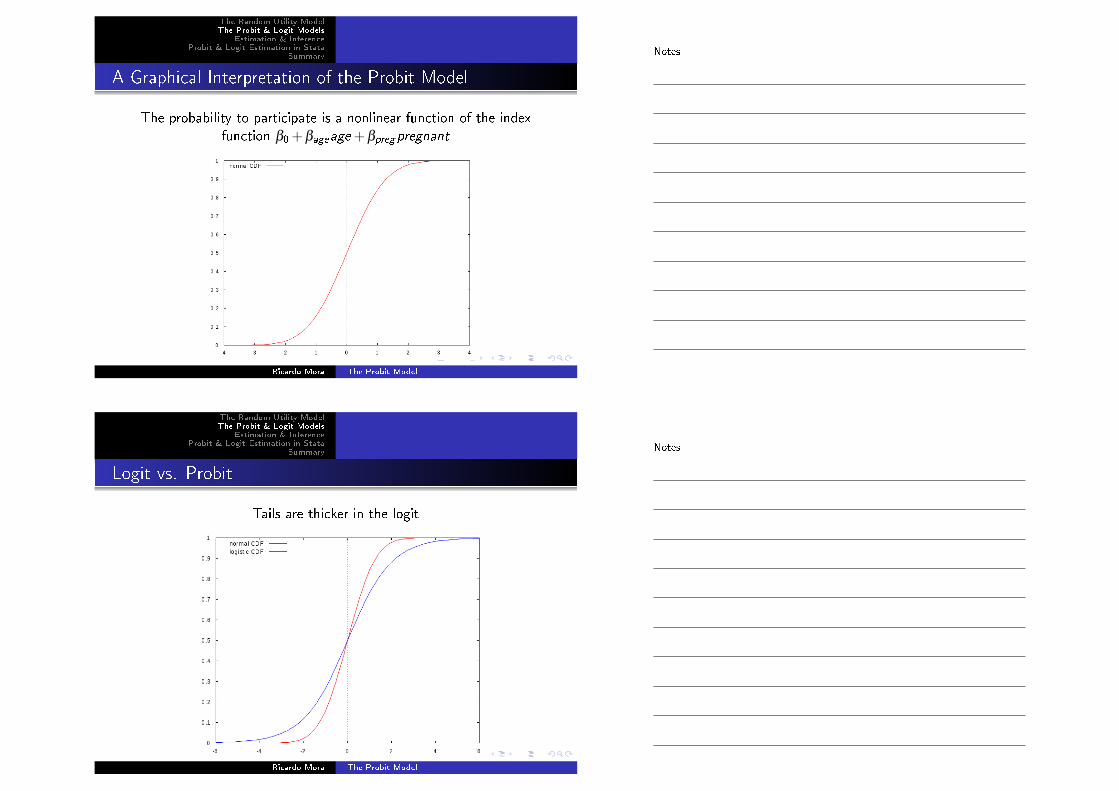
A Graphical Interpretation of the Probit Model

The probability to participate is a nonlinear function of the index

function β0 + βageage + βpregpregnant

Summary

Logit vs. Probit

Tails are thicker in the logit

Summary

Interpretation of the Slopes and Marginal E�ects

when the control xj appears in both utilities...

only the net e�ect on the index function, βj = βjm−β

js , is

identi�ed

normality (nonlinearity) assumption

�net slope� βj captures the marginal e�ect on index function

βx of an increase of one unit of control xj

the marginal e�ect on the probability of marriage is more

complex

if xj is continuous,∂Pr(marry=1)

∂xj= φ (βx)βj

if xj is discrete, ∆Pr(marry = 1) = Φ(βx1)−Φ(βx0)where x1 is the vector of controls with the �nal value for xjand x0 is the vector of controls with the initial value for xj

Summary

js , is

identi�ed

complex

∂xj= φ (βx)βj

Summary

js , is

identi�ed

complex

∂xj= φ (βx)βj

Summary

js , is

identi�ed

complex

∂xj= φ (βx)βj

Summary

js , is

identi�ed

complex

∂xj= φ (βx)βj

Summary

js , is

identi�ed

complex

∂xj= φ (βx)βj

Summary

js , is

identi�ed

complex

∂xj= φ (βx)βj

Summary

The Density in the Probit Model

Assumption: iid random sample

let the true value be β0

then, under the Probit model

Pr(married |x ) =

{Φ(β0x) if marry = 1

1−Φ(β0x) if marry = 0

Summary

Pr(married |x ) =

Summary

Pr(married |x ) =

Summary

The Likelihood of an Observation

the likelihood replaces in the density the true vector β0 with

any vector β

then, the likelihood for individual i takes the form

Li (β ) =

{Φ(βxi ) if marry i = 1

1−Φ(βxi ) if marry i = 0

o, more conveniently,

Li (β ) = [Φ(βxi )]marry i [1−Φ(βxi )](1−marry i )

Summary

any vector β

Li (β ) =

Summary

any vector β

Li (β ) =

Summary

The Loglikelihood

�rst, we take the logs

li (β ) = marry i log (Φ(βxi )) + (1−marryi ) log (1−Φ(βxi ))

then we compute the likelihood for the entire iid sample

l(β ) = ∑ili (β )

l(β ) = ∑i{marryi log (Φ(βxi )) + (1−marryi ) log (1−Φ(βxi ))}

Summary

The Loglikelihood

l(β ) = ∑ili (β )

Summary

The Loglikelihood

l(β ) = ∑ili (β )

Summary

ML Estimation of Probit Model

De�nition

the MLE is the vector βML such that

βML =argmax∑

i{marryi log (Φ(βxi )) + (1−marryi ) log (1−Φ(βxi ))}

because of the nonlinear nature of the maximization problem,

there are not explicit formulas for the probit ML estimates

instead, numerical optimization is used, and, usually, only a

few iterations are needed

in Stata, several algorithms can be used

Summary

De�nition

βML =argmax∑

Summary

De�nition

βML =argmax∑

Summary

De�nition

βML =argmax∑

Summary

The Perfect Prediction Problem

suppose that vector β perfectly predicts marry i in the sense

that for a given scalar k , βx > k i� marry = 1

then the same thing is true for any multiple of β : the sample

identi�cation condition is violated

this may be due to several reasons

one control may be a perfect classi�er: drop itthe model may be trivially misspeci�ed (like predictingmarriage among married individuals)the sample may simply be not large enough

Summary

Asymptotic Properties and Testing

under general conditions, MLE is consistent, asymptotically normal,

and asymptotically e�cient

we can construct (asymptotic) t tests and con�dence intervals

(just as with OLS, 2SLS, and IV)

exclusion restrictions

the Lagrange multiplier or score test only requires estimatingmodel under the nullthe Wald test requires estimation of only the unrestrictedmodelthe likelihood ratio (LR) test requires estimation of bothmodels

Summary

The Likelihood Ratio Test

The LR test

it is based on the di�erence in loglikelihood functions

as with the F tests in linear regression, restricting models leads

to no-larger loglikelihoods

LR = 2(lur − lr )a→ χq

where q is the number of restrictions

Summary

Probit & Logit Estimation in Stata

probit: computes Maximum Likelihood probit estimation

logit: computes Maximum Likelihood logit estimation

margins (mfx): marginal means, predictive margins, marginal

e�ects, and average marginal e�ects

test: Wald tests of simple and composite linear hypothesis

lincom: point estimates, standard errors, testing, and

inference for linear combinations of coe�cients

predict: predictions, residuals, in�uence statistics, and other

diagnostic measures

e(ll): returns the log-likelihood for the last estimated model

We are going to use probit, test, lincom, predict, e(ll), and

Summary

diagnostic measures

Summary

diagnostic measures

Summary

diagnostic measures

Summary

diagnostic measures

Summary

diagnostic measures

Summary

diagnostic measures

Summary

diagnostic measures

Summary

diagnostic measures

Summary

probit depvar indvars [if] [in]

[weight],[options]

depvar : negative is 0, all other nonmissing values is 1

output shows χ2q statistic test for null that all slopes are zero

some interesting options:

noconstant: suppress constant termconstraints(constraints ) apply speci�ed linearconstraints

Summary

[weight],[options]

Summary

[weight],[options]

Summary

[weight],[options]

Summary

A Simulated Example: Participation Decision

The Probit Model

Um = 0.3+0.05∗ educ +0.5∗kids + εm

Uh = 0.8−0.02∗ educ +2∗kids + εh

εh,εm ∼ N (0,Σ) such that ε ∼ N (0,1)

education brings utility if you work, disutility if you don't

having a kid brings more utility if you don't work

βx =−0.5+0.07∗ educ−1.5∗kids

Summary

The Probit Model

Um = 0.3+0.05∗ educ +0.5∗kids + εm

Uh = 0.8−0.02∗ educ +2∗kids + εh

βx =−0.5+0.07∗ educ−1.5∗kids

Summary

The Probit Model

Um = 0.3+0.05∗ educ +0.5∗kids + εm

Uh = 0.8−0.02∗ educ +2∗kids + εh

βx =−0.5+0.07∗ educ−1.5∗kids

Summary

The Probit Model

Um = 0.3+0.05∗ educ +0.5∗kids + εm

Uh = 0.8−0.02∗ educ +2∗kids + εh

βx =−0.5+0.07∗ educ−1.5∗kids

Summary

probit Output

probit work educ kids

Probit regression Number of obs = 5000 LR chi2(2) = 1449.25 Prob > chi2 = 0.0000Log likelihood = -2548.1786 Pseudo R2 = 0.2214

------------------------------------------------------------------------------ work | \Coef. \Std. Err. z P>|z| [95% \Conf. Interval]-------------+---------------------------------------------------------------- educ | .0741842 .0056425 13.15 0.000 .0631251 .0852432 kids | -1.43585 .0409208 -35.09 0.000 -1.516054 -1.355647 _cons | -.5886567 .079498 -7.40 0.000 -.7444698 -.4328435------------------------------------------------------------------------------

Summary

Predicting the Probabilities

Computing Pr (yi = 1 |xi )

predict p_hat ,p

for each observation, if Pr (yi = 1 |xi ) > 0.5 then yi = 1

the percent correctly predicted is the % for which yi matches yi

it is possible to get high percentages correctly predicted in

useless models

suppose that Pr(yi = 0) = 0.9always predicting yi = 0 will lead to 90% correctly predicted!

Summary

predict p_hat ,p

useless models

Summary

predict p_hat ,p

useless models

Summary

predict p_hat ,p

useless models

Summary

predict p_hat ,p

useless models

Summary

predict p_hat ,p

useless models

Summary

Understanding Coe�cients & Marginal E�ects

the column �Coeff.� refers to the ML estimates βML

in contrast to the linear model, in the probit model the

coe�cients do not capture the marginal e�ect on output when

a control changes

if control xj is continuous,∂Pr(y=1)

∂xj= φ (βx)βj

if control xj is discrete, ∆Pr (work = 1) = Φ(βx1)−Φ(βx0)

since the model is non-linear, marginal e�ects depend on the

values of the other controls

to get marginal e�ects instead of coe�cients we can use

command dprobit

we can also use the commands margins or mfx

Summary

a control changes

∂xj= φ (βx)βj

command dprobit

Summary

a control changes

∂xj= φ (βx)βj

command dprobit

Summary

a control changes

∂xj= φ (βx)βj

command dprobit

Summary

a control changes

∂xj= φ (βx)βj

command dprobit

Summary

a control changes

∂xj= φ (βx)βj

command dprobit

Summary

dprobit work educ kids

Probit regression, reporting marginal effects Number of obs = 5000 LR chi2(2) =1449.25 Prob > chi2 = 0.0000Log likelihood = -2548.178\6 Pseudo R2 = 0.2214

------------------------------------------------------------------------------ \work | dF/dx Std. Err. z P>|z| x-bar [ 95% C.I. ]---------+-------------------------------------------------------------------- educ | .02\68932 .0020397 13.15 0.000 13.5\644 .022895 .030891 kids*| -.507\601\6 .012\6823 -35.09 0.000 .595\6 -.532458 -.482745---------+-------------------------------------------------------------------- obs. P | .3\62 pred. P | .3308434 (at x-bar)------------------------------------------------------------------------------(*) dF/dx is for discrete change of dummy variable from 0 to 1 z and P>|z| correspond to the test of the underlying coefficient being 0

Summary

Individual Marginal E�ects: Discrete Change

we want to estimate the change in probability when x changes from

x0 to x1

Discrete change

after estimation of the model, predict index function βMLx0

replace values in controls from scenario 0, x0, to scenario 1, x1

predict index function βMLx1

generate the individual marginal e�ects

βMLx1

)−Φ

(βMLx0

)Ricardo Mora The Probit Model

Summary

Individual Marginal E�ects: Discrete Change

we want to estimate the change in probability when x changes from

x0 to x1

Discrete change

after estimation of the model, predict index function βMLx0

replace values in controls from scenario 0, x0, to scenario 1, x1

predict index function βMLx1

generate the individual marginal e�ects

βMLx1

)−Φ

(βMLx0

)Ricardo Mora The Probit Model

Summary

Example: The E�ect of Having A Kid

// marginal effects of having a kidgen kids_old=kidsreplace kids=1predict p1,preplace kids=0predict p0,pgen Mg_kid = p1 - p0bysort educ: sum Mg_kid

Summary

bysort educ : su Mg_kid

-> educ = 8

Variable | Obs Mean Std. Dev. Min Max-------------+-------------------------------------------------------- Mg_kid | 721 -.4257113 0 -.4257113 -.4257113

-> educ = 12

-> educ = 16

-> educ = 21

the e�ect of having a kid changes with education

higher education makes individuals more likely to have indexes

βx closer to 0.5 (the probit slope is largest at 0.5)

how would you make the �kid� e�ect smaller with higher

education?

Summary

-> educ = 8

-> educ = 12

-> educ = 16

-> educ = 21

education?

Summary

-> educ = 8

-> educ = 12

-> educ = 16

-> educ = 21

education?

Summary

-> educ = 8

-> educ = 12

-> educ = 16

-> educ = 21

education?

Summary

Individual Marginal E�ects: In�nitessimal Change

Calculus approximation

after estimation, predict the index function βMLx

generate the calculus approximation: φ

(βMLx

)βMLj

Summary

Example of Calculus Approximation

On individual values

// marginal effects of one extra year of education (individual calculus approximation). predict xb_hat,xb. gen Mg_educ_cal=normalden(xb_hat)*_b[educ] // this is the individual's marginal effect. su Mg_educ_cal

Variable | Obs Mean Std. Dev. Min Max-------------+-------------------------------------------------------- Mg_educ_cal | 5000 .0212441 .0058988 .01063 .0295949

On average values

. // marginal effects of one extra year of education (at the mean values)

. rename educ educ_old

. rename kids kids_old

. egen educ = mean(educ_old) if e(sample)

. egen kids = mean(kids_old) if e(sample)

. predict xb_hat_avg,xb

. gen Mg_educ_avg=normalden(xb_hat_avg)*_b[educ] // this is the marginal effect on averages

. su Mg_educ_avg

Variable | Obs Mean Std. Dev. Min Max-------------+-------------------------------------------------------- Mg_educ_avg | 5000 .0268932 0 .0268932 .0268932

Summary

Logit Estimation

logit educ kids

Logistic regression Number of obs = 5000 LR chi2(2) = 1446.73 Prob > chi2 = 0.0000Log likelihood = -2549.4381 Pseudo R2 = 0.2210

------------------------------------------------------------------------------ work \| \Coef. Std. Err. z P>\|z\| [95% \Conf. Interval]-------------+---------------------------------------------------------------- educ \| .1263039 .0097563 12.95 0.000 .1071819 .1454258 kids \| -2.386564 .0715243 -33.37 0.000 -2.526749 -2.246379 _cons \| -1.031709 .1346306 -7.66 0.000 -1.295581 -.7678384------------------------------------------------------------------------------

Marginal effects after logit y = Pr(work) (predict) = .32302366------------------------------------------------------------------------------variable | dy/dx Std. Err. z P>|z| [ \9\5% C.I. ] X---------+-------------------------------------------------------------------- educ | .02762 .00212 13.02 0.000 .023462 .031778 13.\5644 kids*| -.\5102708 .01283 -3\9.78 0.000 -.\53\5413 -.48\512\9 .\5\9\56------------------------------------------------------------------------------(*) dy/dx is for discrete change of dummy variable from 0 to 1

Logit & Probit β are not comparable, but marginal e�ects are.

Summary

not all parameters of the RUM can be estimated

the Probit and Logit models identify how each control a�ects

the probability of participation

ML estimation requires numerical methods

under general conditions, ML estimates are consistent,

asymptotically normal, and asymptotically e�cient

signi�cance tests and general restrictions tests are easy to

carry out with the Probit model

Stata allows for probit and logit estimation of the random

utility model by ML

the probit & logit models - departamento de...

Documents