regression models for categorical dependent variables ...course overview (continued) thursday...
TRANSCRIPT

Regression Models for Categorical DependentVariables (Logit, Probit, and Related Techniques)
ZA Spring Seminar 2008
Andreas Diekmann Ben Jann
ETH ZurichSwitzerland
Cologne, February 25–29, 2008
Diekmann/Jann (ETH Zurich) Regression Models for Categorical Data ZA Spring Seminar 2008 1 / 188

Categorical Dependent Variables: Examples
Participation in elections (no = 0, yes = 1)
Voting in a multi-party system (polytomous variable)
Labor force participation (no = 0, yes = 1; or: no = 0, part-time = 1,full-time = 2)
Union membership
Purchase of a durable consumer good in a certain time span
Successfully selling a good on eBay
Victim of a crime in last 12 month
Divorce within five years after marriage
Number of children
Choice of traffic mode (by car = 0, public transportation = 1; or: byfoot = 0, by bike = 1, public transportation = 2, by car = 3)
Life satisfaction on a scale from 1 to 5
Diekmann/Jann (ETH Zurich) Regression Models for Categorical Data ZA Spring Seminar 2008 2 / 188

Categorical Dependent Variables: Models
Dependent Variable Method
continuous, unbounded linear regression (OLS)
binary (dichotomous) logistic regression, probit, and related mod-els
nominal (polytomous) multinomial logit, conditional logit
ordered outcomes ordered logit/probit, and related models
count data poisson regression, negative binomial re-gression, and related models
limited/bounded censored regression (e.g. Tobit)
(censored) duration data survival models, event history analysis (e.g.Cox regression)
Independent Variables: metric and/or dichotomous
Diekmann/Jann (ETH Zurich) Regression Models for Categorical Data ZA Spring Seminar 2008 3 / 188

Multivariate Methods 1.pdf
Why multivariate methodswith categorical or other types
of variables?
Diekmann/Jann (ETH Zurich) Regression Models for Categorical Data ZA Spring Seminar 2008 4 / 188
Multivariate Methods 2.pdf
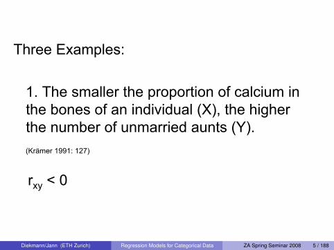
Three Examples:
1. The smaller the proportion of calcium in the bones of an individual (X), the higherthe number of unmarried aunts (Y). (Krämer 1991: 127)
rxy < 0
Diekmann/Jann (ETH Zurich) Regression Models for Categorical Data ZA Spring Seminar 2008 5 / 188

Multivariate Methods 3.pdf
2. The larger the size of shoes (X), thehigher the income (Y).
rxy > 0
Diekmann/Jann (ETH Zurich) Regression Models for Categorical Data ZA Spring Seminar 2008 6 / 188

Multivariate Methods 4.pdf
3. The larger a fire brigade, i. e. the morefirefighters (X), the higher the damage bythe fire (Y).(Paul Lazarsfeld)
rxy > 0
Diekmann/Jann (ETH Zurich) Regression Models for Categorical Data ZA Spring Seminar 2008 7 / 188

Multivariate Methods 5.pdf
X (calcium)+
Z (AGE) rxy < 0-
Y (unmarried aunts)
Diekmann/Jann (ETH Zurich) Regression Models for Categorical Data ZA Spring Seminar 2008 8 / 188
Multivariate Methods 6.pdf
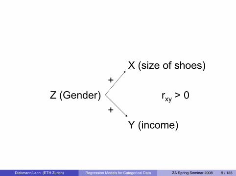
X (size of shoes)+
Z (Gender) rxy > 0+
Y (income)
Diekmann/Jann (ETH Zurich) Regression Models for Categorical Data ZA Spring Seminar 2008 9 / 188

Multivariate Methods 7.pdf
X (firefighters)+
Z (fire) - rxy > 0+
Y (damage)
Diekmann/Jann (ETH Zurich) Regression Models for Categorical Data ZA Spring Seminar 2008 10 / 188

Multivariate Methods 8.pdf
Experimental approach:
Control (small number of firefighters)Experimental factor (large number of firefighters)
Essential: Randomization
x1 o1 Rx2 o2 R
Neutralization of other factors z1, z2, z3, …byrandomization!
Diekmann/Jann (ETH Zurich) Regression Models for Categorical Data ZA Spring Seminar 2008 11 / 188

Multivariate Methods 9.pdf
Serious problem in evaluation researchFor example:
1. Labour Market: Occupational training and career success
2. Educational policies: Comparing state and private schools
3. Health policy: SWICA study: Fitness training and healthconditions
4. Criminology: Imprisonment versus community work and recidivism rates
Causal effect or selection effect?
Diekmann/Jann (ETH Zurich) Regression Models for Categorical Data ZA Spring Seminar 2008 12 / 188

Multivariate Methods 10.pdf
If experimental designs are not applicable:Multivariate statistics
1. Which other factors besides X and Y may berelevant? (Theory)
2. Other factors have to be measured.
3. Include relevant other factors („controls“) in a statistical model
Diekmann/Jann (ETH Zurich) Regression Models for Categorical Data ZA Spring Seminar 2008 13 / 188

Multivariate Methods 11.pdf
Linear Modely = b0 + b1x + b2z + εrxy > 0, b1 = 0, b2 > 0 („spurious correlation“)
byx = [sy/sx] (rxy – rxz • ryz) / (1 – r2xy)
rxy > 0, b1 = 0 rxy = rxz • ryz
More general case:
y = b0 + b1x1 + b2x2 + …+ bmxm + ε
Diekmann/Jann (ETH Zurich) Regression Models for Categorical Data ZA Spring Seminar 2008 14 / 188

Multivariate Methods 12.pdf
Simple method: Split of bivariate tables bycontrol variables (multivariate tableanalysis)
Problem: Easy, if one dichotomous controlvariable. Otherwise, a large data set isnecessary.
Diekmann/Jann (ETH Zurich) Regression Models for Categorical Data ZA Spring Seminar 2008 15 / 188

Multivariate Methods 13.pdf
Multivariate analysis: Example with three categorical
variables
Diekmann/Jann (ETH Zurich) Regression Models for Categorical Data ZA Spring Seminar 2008 16 / 188

Multivariate Methods 14.pdf
Diekmann/Jann (ETH Zurich) Regression Models for Categorical Data ZA Spring Seminar 2008 17 / 188

Multivariate Methods 15.pdf
Diekmann/Jann (ETH Zurich) Regression Models for Categorical Data ZA Spring Seminar 2008 18 / 188

Multivariate Methods 16.pdf
By Sex
Men Women
Mortality
Diekmann/Jann (ETH Zurich) Regression Models for Categorical Data ZA Spring Seminar 2008 19 / 188

Multivariate Methods 17.pdf
Social class
Men
Diekmann/Jann (ETH Zurich) Regression Models for Categorical Data ZA Spring Seminar 2008 20 / 188

Multivariate Methods 18.pdf
Sex
Mortality
Social Class
Interaction ofSex and class
Multicausality andinteraction
Women
Diekmann/Jann (ETH Zurich) Regression Models for Categorical Data ZA Spring Seminar 2008 21 / 188

Multivariate Methods 19.pdf
Male, III. Classdied
Female, I. Classsurvived
Diekmann/Jann (ETH Zurich) Regression Models for Categorical Data ZA Spring Seminar 2008 22 / 188

Course overview
MondayMorning: Lecture (Diekmann)
I Introduction and overviewI Linear regression (OLS)I Linear probability model (LPM)I Logistic regression model
Afternoon: Lecture (Diekmann)I Logistic regression: Interpretation of coefficientsI Maximum-likelihood estimation (MLE) of parameters
TuesdayMorning and afternoon: PC Pool (Jann)
I Introduction to software (SPSS and Stata) and data filesI Exercises for LPM and logistic regressionI Post processing of results: Interpretation of coefficientsI Post processing of results: Tabulation
Diekmann/Jann (ETH Zurich) Regression Models for Categorical Data ZA Spring Seminar 2008 23 / 188

Course overview (continued)
WednesdayMorning: Lecture (Jann)
I Statistical inference: Wald-test and likelihood-ratio test (LR)I Evaluation of models: Goodness-of-fit measures (GOF)I Model specificationI Model diagnostics
Afternoon: PC Pool (Jann)I Exercises: Statistical inference, goodness-of-fit, specification,
diagnostics
Diekmann/Jann (ETH Zurich) Regression Models for Categorical Data ZA Spring Seminar 2008 24 / 188

Course overview (continued)
Thursday
Morning: Lecture (Jann)I Probit modelI Logit/Probit as latent variable models and derivation from utility
assumptionsI Ordered Logit and Probit, multinomial and conditional Logit
Afternoon: PC Pool (Jann)I Exercises for Probit, ordered Logit/Probit, multinomial and conditional
Logit
Friday
Morning: Lecture (Jann)I Outlook: Models for count data, panel data models, other topicsI Final discussion
Diekmann/Jann (ETH Zurich) Regression Models for Categorical Data ZA Spring Seminar 2008 25 / 188

Textbooks and Overview Articles: EnglishAldrich, John H., and Forrest D. Nelson (1984). Linear Probability, Logit, and ProbitModels. Newbury Park, CA: Sage.
Amemiya, Takeshi (1981). Qualitative Response Models: A Survey. Journal ofEconomic Literature 19(4): 1483-1536.
Borooah, Vani K. (2002). Logit and Probit. Ordered and Multinomial Models.Newbury Park, CA: Sage.
Eliason, Scott R. (1993). Maximum Likelihood Estimation. Logic and Practice.Newbury Park, CA: Sage.
Fox, John (1997). Applied Regression Analysis, Linear Models, and RelatedMethods. Thousand Oaks, CA: Sage. (Chapter 15)
Greene, William H. (2003). Econometric Analysis. 5th ed. Upper Saddle River, NJ:Pearson Education. (Chapter 21)
Gujarati, Damodar N. (2003). Basic Econometrics. 4th ed. New York: McGraw-Hill.(Chapter 15)
Hosmer, David W., Jr., and Stanley Lemeshow (2000). Applied Logistic Regression.2nd ed. New York: John Wiley & Sons.
Jaccard, James (2001). Interaction Effects in Logistic Regression. Newbury Park,CA: Sage.
Diekmann/Jann (ETH Zurich) Regression Models for Categorical Data ZA Spring Seminar 2008 26 / 188

Textbooks and Overview Articles: EnglishKohler, Ulrich, and Frauke Kreuter (2005). Data Analysis Using Stata. 2nd ed.College Station, TX: Stata Press. (Chapter 9)Liao, Tim Futing (1994). Interpreting Probability Models. Logit, Probit, and OtherGeneralized Linear Models. Newbury Park, CA: Sage.Long, J. Scott (1997). Regression Models for Categorical and Limited DependentVariables. Thousand Oaks, CA: Sage.Long, J. Scott, and Jeremy Freese (2005). Regression Models for CategoricalDependent Variables Using Stata. College Station, TX: Stata Press.Maddala, G. S. (1983). Limited Dependent and Qualitative Variables inEconometrics. Cambridge: Cambridge University Press.Menard, Scott (2002). Applied Logistic Regression Analysis. 2nd ed. Newbury Park,CA: Sage.Pampel, Fred C. (2000). Logistic Regression. A Primer. Newbury Park, CA: Sage.Verbeek, Marno (2004). A Guide to Modern Econometrics. West Sussex: John Wiley& Sons. (Chapter 7)Winship, Christopher, and Robert D. Mare (1984). Regression Models with OrdinalVariables. American Sociological Review 49(4): 512-525.Wooldridge, Jeffrey M. (2002). Econometric Analysis of Cross Section and PanelData. Cambridge, MA: The MIT Press. (Chapter 15)
Diekmann/Jann (ETH Zurich) Regression Models for Categorical Data ZA Spring Seminar 2008 27 / 188

Textbooks and Overview Articles: German
Andreß, Hans-Jurgen, Jacques A. Hagenaars, und Steffen Kuhnel (1997). Analysevon Tabellen und kategorialen Daten. Log-lineare Modelle, latente Klassenanalyse,logistische Regression und GSK-Ansatz. Berlin: Springer.
Bruderl, Josef (2000). Regressionsverfahren in der Bevolkerungswissenschaft. S.589-642 in: Ulrich Mueller, Bernhard Nauck, and Andreas Diekmann (Hg.).Handbuch der Demographie. Berlin: Springer. (Abschnitt 13.2)
Backhaus, Klaus, Bernd Erichson, Wulff Plinke, und Rolf Weiber (2006). MultivariateAnalysemethoden. Eine anwendungsorientierte Einfuhrung. 11. Aufl. Berlin:Springer. (Kapitel 7)
Kohler, Ulrich, und Frauke Kreuter (2006). Datenanalyse mit Stata. AllgemeineKonzepte der Datenanalyse und ihre praktische Anwendung. 2. Aufl. Munchen:Oldenbourg. (Kapitel 9)
Maier, Gunther, und Peter Weiss (1990). Modelle diskreter Entscheidungen: Theorieund Anwendung in den Sozial- und Wirtschaftswissenschaften. Wien: Springer.
Tutz, Gerhard (2000). Die Analyse kategorialer Daten. AnwendungsorientierteEinfuhrung in Logit-Modellierung und kategoriale Regression. Munchen:Oldenbourg.
Diekmann/Jann (ETH Zurich) Regression Models for Categorical Data ZA Spring Seminar 2008 28 / 188

General Statistics Textbooks
English:
Agresti, Alan, and Barbara Finlay (1997). Statistical Methods for the Social Sciences.Third Edition. Upper Saddle River, NJ: Prentice-Hall.
Freedman, David, Robert Pisani, and Roger Purves (1998). Statistics. Third Edition.New York: Norton.
German:
Fahrmeir, Ludwig, Rita Kunstler, Iris Pigeot, and Gerhard Tutz (2004). Statistik. DerWeg zur Datenanalyse. 5. Auflage. Berlin: Springer.
Jann, Ben (2005). Einfuhrung in die Statistik. 2. Auflage. Munchen: Oldenbourg.
Diekmann/Jann (ETH Zurich) Regression Models for Categorical Data ZA Spring Seminar 2008 29 / 188

Part I
General Statistical Concepts
Probability and Random Variables
Probability Distributions
Parameter Estimation
Expected Value and Variance
Diekmann/Jann (ETH Zurich) Regression Models for Categorical Data ZA Spring Seminar 2008 30 / 188

Probability and Random VariablesGiven is a random process with possible outcomes A , B, etc. Theprobability Pr(A) is the relative expected frequency of event A .
Probability axioms:
Pr(A) ≥ 0
Pr(Ω) = 1
Pr(A ∪ B) = Pr(A) + Pr(B) if A ∩ B = ∅
where Ω is the set of (disjunctive) elementary outcomes.
Conditional probability Pr(A |B): Probability of A given the occurrenceof B
A random variable is a variable that takes on different values withcertain probabilities.Imagine tossing a coin. The outcome of the toss is a random variable.There are two possible outcomes, heads and tails, and each outcomehas probability 0.5.
Diekmann/Jann (ETH Zurich) Regression Models for Categorical Data ZA Spring Seminar 2008 31 / 188

Probability Distribution
A random variable can be discrete (only selected values arepossible) or continuous (any value in an interval is possible).
The probability distribution of a random variable X can be expressedas probability mass or density function (PDF) or as cumulativeprobability function (CDF).
PDFdiscrete: f(x) = p(x) = Pr(X = x)
continuous: Pr(a ≤ X ≤ b) =∫ b
a f(x) dx
CDFdiscrete: F(x) = Pr(X ≤ x) =
∑xi≤x p(xi)
continuous: F(x) = Pr(X ≤ x) =∫ x−∞
f(t) dt
Diekmann/Jann (ETH Zurich) Regression Models for Categorical Data ZA Spring Seminar 2008 32 / 188

Probability Distribution: Example
Normal distribution and density (continuous)
0.2
.4.6
.81
−4 −2 0 2 4x
F(x)f(x)
f(x) = φ(x |µ, σ) =1
σ√
2πe−
(x−µ)2
2σ2
Diekmann/Jann (ETH Zurich) Regression Models for Categorical Data ZA Spring Seminar 2008 33 / 188

Parameter Estimation
Distributions can be described by parameters such as the expectedvalue (the mean) or the variance. The goal in statistics is to estimatethese parameters based on sample data.
Desirable properties of an estimator θ for parameter vector θ:1 Unbiasedness: E(θ) = θ – on average (over many samples) the
estimator is equal to the true θ.
2 Efficiency: The variance of the estimator (i.e. the variability of theestimates from sample to sample) should be as small as possible.
3 Consistency: Unbiasedness is not always possible, but an estimatorshould at least be asymptotically unbiased (i.e. E(θ) should approach θas n → ∞).
The sampling variance of an estimator determines the precision ofthe estimator and can be used to construct confidence intervals andsignificance tests. (The sampling variance itself is also unknown andhas to be estimated.)
Diekmann/Jann (ETH Zurich) Regression Models for Categorical Data ZA Spring Seminar 2008 34 / 188

Expected Value and Variance
Expected Value E(X) = µ
discrete: E(X) =∑
i
xip(xi) continuous: E(X) =
∫ +∞
−∞
xf(x) dx
Variance V(X) = σ2
general: V(X) = E[(X − µ)2] = E(X2) − µ2
discrete: V(X) =∑
i
(xi − µ)2p(xi) cont.: V(X) =
∫ +∞
−∞
(x − µ)2f(x) dx
Sample estimators X and SX
E(X) = X =1N
N∑i=1
Xi V(X) = SX =1
N − 1
N∑i=1
(Xi − X)2
Diekmann/Jann (ETH Zurich) Regression Models for Categorical Data ZA Spring Seminar 2008 35 / 188
Part II
Multiple Linear Regression
Model
Assumptions
Interpretation
Estimation
Goodness-of-Fit
Diekmann/Jann (ETH Zurich) Regression Models for Categorical Data ZA Spring Seminar 2008 36 / 188
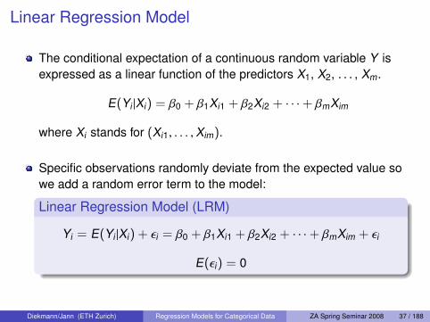
Linear Regression Model
The conditional expectation of a continuous random variable Y isexpressed as a linear function of the predictors X1, X2, . . . , Xm.
E(Yi |Xi) = β0 + β1Xi1 + β2Xi2 + · · ·+ βmXim
where Xi stands for (Xi1, . . . ,Xim).
Specific observations randomly deviate from the expected value sowe add a random error term to the model:
Linear Regression Model (LRM)
Yi = E(Yi |Xi) + εi = β0 + β1Xi1 + β2Xi2 + · · ·+ βmXim + εi
E(εi) = 0
Diekmann/Jann (ETH Zurich) Regression Models for Categorical Data ZA Spring Seminar 2008 37 / 188

Linear Regression Model
LRM in Matrix Notation
Y = Xβ+ εY1
Y2...
Yn
=
1 X11 X12 · · · X1m
1 X21 X22 · · · X2m......
.... . .
...
1 Xn1 Xn2 · · · Xnm
β0
β1
β2...
βm
+
ε1ε2...
εn
Diekmann/Jann (ETH Zurich) Regression Models for Categorical Data ZA Spring Seminar 2008 38 / 188

Graphical RepresentationSimple LRM
X
Y
E(Yi)
E(Yi) = α + βxiεi
α
β
yi
xi1 2
Diekmann/Jann (ETH Zurich) Regression Models for Categorical Data ZA Spring Seminar 2008 39 / 188

Assumptions1 Conditional expectation of error term is zero
E(εi) = 0
This impliesE(Yi |Xi) = X ′i β
and also that the errors and predictors are uncorrelated:
E(εiXik ) = 0
(correct functional form, no relevant omitted variables, no reversecausality/endogeneity)
2 The errors have constant variance and are uncorrelated
E(εε′) = σ2I
3 Errors are normally distributed:
εi ∼ N(0, σ)
Diekmann/Jann (ETH Zurich) Regression Models for Categorical Data ZA Spring Seminar 2008 40 / 188

Assumptions
X
X1
X2
X3
X4
Y
f (ε)
Y = β0 + β1X
Diekmann/Jann (ETH Zurich) Regression Models for Categorical Data ZA Spring Seminar 2008 41 / 188

Heteroscedasticity0
24
68
10
Y1
1 2 3 4 5
X
Homoscedasticity
02
46
810
Y2
1 2 3 4 5
X
Heteroscedasticity
Diekmann/Jann (ETH Zurich) Regression Models for Categorical Data ZA Spring Seminar 2008 42 / 188

Interpretation
Model:E(Y |X) = β0 + β1X1 + β2X2 + · · ·+ βmXm
Marginal Effect / Partial Effect
∂E(Y |X)
∂Xk= βk
Discrete Change / Unit Effect (effect of ∆Xk = 1)
∆E(Y |X)
∆Xk= E(Y |X ,Xk + 1) − E(Y |X ,Xk ) = βk
In linear regression: marginal effect = unit effect
⇒ effects are independent of value of Xk and Y (constant effects)⇒ very convenient for interpretation
Diekmann/Jann (ETH Zurich) Regression Models for Categorical Data ZA Spring Seminar 2008 43 / 188
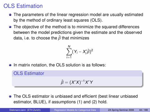
OLS EstimationThe parameters of the linear regression model are usually estimatedby the method of ordinary least squares (OLS).The objective of the method is to minimize the squared differencesbetween the model predictions given the estimate and the observeddata, i.e. to choose the β that minimizes
N∑i=1
(Yi − X ′i β)2
In matrix notation, the OLS solution is as follows:
OLS Estimator
β = (X ′X)−1X ′Y
The OLS estimator is unbiased and efficient (best linear unbiasedestimator, BLUE), if assumptions (1) and (2) hold.
Diekmann/Jann (ETH Zurich) Regression Models for Categorical Data ZA Spring Seminar 2008 44 / 188

Residuals and R-SquaredPredictions based on estimated parameters:
Yi = β0 + β1Xi1 + · · ·+ βmXim
Residuals: Deviation between predictions and observed data
ri = Yi − Yi = Yi − β0 − β1Xi1 − · · · − βmXim
The mechanics of OLS are such that the sum of residuals is zero andthe sum of squared residuals is minimized.As a measure of goodness-of-fit between the data and the model,the R-squared is used: Proportion of variance of Y which is“explained” by the model.
R-squared
R2 =
∑Ni=1(Yi − Y)2∑Ni=1(Yi − Y)2
= 1 −
∑Ni=1 r2
i∑Ni=1(Yi − Y)2
Diekmann/Jann (ETH Zurich) Regression Models for Categorical Data ZA Spring Seminar 2008 45 / 188

Part III
Linear Probability Model (LPM)
Model
Advantages
Example
Problems
WLS estimation
Diekmann/Jann (ETH Zurich) Regression Models for Categorical Data ZA Spring Seminar 2008 46 / 188

Linear Probability Model (LPM)
Given is a dichotomous (binary) dependent variable Y :
Yi =
1 Event
0 No event
Expected value: The probability distribution of Y is given asPr(Yi = 1) = πi for value 1 und Pr(Yi = 0) = (1 − πi) for value 0,πi ∈ [0, 1], therefore
E(Yi) = 1 · πi + 0 · (1 − πi) = Pr(Yi = 1)
⇒ the expected value of Y is equal to the probability of Y being 1
Diekmann/Jann (ETH Zurich) Regression Models for Categorical Data ZA Spring Seminar 2008 47 / 188

Linear Probability Model (LPM)
Because E(Yi) = Pr(Yi = 1) it seems reasonable to modelPr(Yi = 1) using standard linear regression techniques:
Pr(Yi = 1|Xi) = E(Yi |Xi) = β0 + β1Xi1 + β2Xi2 + · · ·+ βmXim
Adding the error term yields the Linear Probability Model, whichmodels Pr(Yi = 1) as a linear function of the independent variables:
Linear Probability Model (LPM)
Yi = Pr(Yi = 1|Xi) + εi = E(Yi |Xi) + εi
= β0 + β1Xi1 + β2Xi2 + · · ·+ βmXim + εi
where E(εi) = 0 is assumed.
The model parameters can be estimated using OLS.
Diekmann/Jann (ETH Zurich) Regression Models for Categorical Data ZA Spring Seminar 2008 48 / 188

Are the OLS parameter estimates unbiased?
The model isYi = Pr(Yi = 1|Xi) + εi = Zi + εi
whereZi = β0 + β1Xi1 + · · ·+ βmXim
Therefore:
εi =
−Zi if Yi = 0
1 − Zi if Yi = 1
It follows:
E(εi) = Pr(Yi = 0|Xi)(−Zi) + Pr(Yi = 1|Xi)(1 − Zi) = 0
because Pr(Yi = 1|Xi) = Zi by definition. Since E(εi) = 0, the OLSestimates are unbiased. (Depending on the model being correct!)
Diekmann/Jann (ETH Zurich) Regression Models for Categorical Data ZA Spring Seminar 2008 49 / 188

Advantages of the LPM
Easy to interpret:I βk is the expected change in Pr(Y = 1) for a unit increase in Xk
Pr(Y = 1|Xk + 1)) − Pr(Y = 1|Xk ) = βk
I βk is the partial (marginal) effect of Xk on Pr(Y = 1)
∂Pr(Y = 1|X)
∂Xk= βk
Simple to estimate via OLS.
Good small sample behavior.
Often good as a first approximation, especially if the mean ofPr(Y = 1) is not close to 0 or 1 and effects are not too strong.
Applicable in cases where the Logit (or similar) fails (e.g. if Y constantfor one value of a categorical predictor, see Caudill 1988; in badlybehaved Randomized Response data)
Diekmann/Jann (ETH Zurich) Regression Models for Categorical Data ZA Spring Seminar 2008 50 / 188

Polytomous dependent variable
LPM can also be used to model a polytomous variable that has J > 2categories (e.g. religious denomination).
One equation is estimated for each category, i.e.
Yi1 = β01 + β11 + Xi + · · ·+ εi1
Yi2 = β02 + β12 + Xi + · · ·+ εi2...
YiJ = β0J + β1J + Xi + · · ·+ εiJ
where YiJ =
1 if Yi = j
0 else
As long as constants are included in the separate models, OLS ensuresthat
J∑j=1
Yij =J∑
j=1
(β0j + β1j + Xi + · · ·+) = 1
Diekmann/Jann (ETH Zurich) Regression Models for Categorical Data ZA Spring Seminar 2008 51 / 188

Example of the LPM: Labor Force Participation (Long1997:36-38)
Diekmann/Jann (ETH Zurich) Regression Models for Categorical Data ZA Spring Seminar 2008 52 / 188

Example of the LPM: Labor Force Participation (Long1997:36-38)
Diekmann/Jann (ETH Zurich) Regression Models for Categorical Data ZA Spring Seminar 2008 53 / 188

Problems of LPM
Nonsensical predictions. Predictions from the LPM can be below 0or above 1, which contradicts Kolmogorov’s probability axioms.
1
0
Y
X
LPM
B
A
1
0
Y
X
Truncated LPM
B
A
Unreasonable functional form. The LPM assumes that effects arethe same over the whole probability range, but this is often notrealistic.
Usefulness of R2 is questionable. Even a very clear relationships donot result in a high R2-values.
Diekmann/Jann (ETH Zurich) Regression Models for Categorical Data ZA Spring Seminar 2008 54 / 188

Problems of LPM
Nonnormality. The errors are not normally distributed in the LPM,since εi can only have two values: −Zi or 1 − Zi .Consequences:
I normal-approximation inference is invalid in small samplesI more efficient non-linear estimators exist (LPM is not BUE)
Heteroskedasticity. The errors are do not have constant variance
V(εi) = E(ε2i ) = Pr(Yi = 0)[−Zi]2 + Pr(Yi = 1)[1 − Zi]
2
= [1 − Pr(Yi = 1)][Pr(Yi = 1)]2 + Pr(Yi = 1)[1 − Pr(Yi = 1)]2
= Pr(Yi = 1)[1 − Pr(Yi = 1)] = Zi(1 − Zi)
since E(εi) = 0 and Pr(Yi = 1) = Zi = β0 + β1Xi1 + · · ·+ βmXim.
⇒ OLS estimator is inefficient (and standard errors are biased)
Diekmann/Jann (ETH Zurich) Regression Models for Categorical Data ZA Spring Seminar 2008 55 / 188

WLS estimation of LPMGoldberger (1964) proposed to use a two-step, weighted leastsquared approach (WLS) to correct for heteroskedasticity.
I Step 1: Estimate standard OLS-LPM to obtain an estimate of the errorvariance
V(εi) = Yi(1 − Yi), Yi = β0 + β1Xi1 + · · ·+ βmXim
I Step 2: Use the estimated variance in a weighted least squaresapproach to estimate the heteroskedasticity-corrected LPMparameters. (Intuitively: smaller variance, more reliable observation.)This is equivalent to dividing all variables (including the constant) bythe square-root of the variance and then fit an OLS model to thesemodified data.
wiYi = β0wi + β1wiXi1 + · · ·+ εiwi , wi =
√Yi(1 − Yi)−1
The procedure increases the efficiency of the LPM (but standarderrors are still somewhat biased since the true variance is unknown).Problematic are observations for which Yi is outside [0, 1] (negativevariance estimate!).
Diekmann/Jann (ETH Zurich) Regression Models for Categorical Data ZA Spring Seminar 2008 56 / 188

Part IV
Logistic Regression: Model
Nonlinear Relationship
The Logit Model
Log Odds Form
Simple Example
Diekmann/Jann (ETH Zurich) Regression Models for Categorical Data ZA Spring Seminar 2008 57 / 188

Nonlinear Effect on P(Y = 1)
The linear effects assumed in the LPM do often not make muchsense and a more reasonable probability model should
1 ensure that Pr(Y = 1) always lies within [0, 1] and2 use a nonlinear functional form so that effects diminish if Pr(Yi = 1)
gets close to 0 or 1
Usually it is also sensible to assume symmetry.
Example for such a nonlinear function:
1
0
P
X
Diekmann/Jann (ETH Zurich) Regression Models for Categorical Data ZA Spring Seminar 2008 58 / 188

The Logit Model
A suitable function to model the relationship between Pr(Yi = 1) and theindependent variables is the logistic function.
The logistic function
Y =eZ
1 + eZ=
11 + e−Z
Parameterizing Z as a linear function of the predictors yields the Logitmodel.
The Logit Model
Pr(Yi = 1|Xi) = E(Yi |Xi) =1
1 + e−Zi=
11 + e−(β0+β1Xi1+···+βmXim)
Diekmann/Jann (ETH Zurich) Regression Models for Categorical Data ZA Spring Seminar 2008 59 / 188
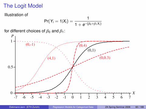
The Logit Model
Illustration ofPr(Yi = 1|Xi) =
11 + e−(β0+β1Xi)
for different choices of β0 and β1:
-7 -6 -5 -4 -3 -2 -1 0 1 2 3 4 5 6 7
0
0.5
1
X
P
(0,1)
(0,4)
(0,0.3)
(0,-1)
(4,1)
Diekmann/Jann (ETH Zurich) Regression Models for Categorical Data ZA Spring Seminar 2008 60 / 188
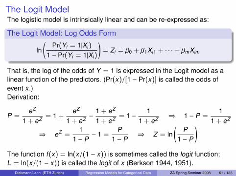
The Logit ModelThe logistic model is intrinsically linear and can be re-expressed as:
The Logit Model: Log Odds Form
ln(
Pr(Yi = 1|Xi)
1 − Pr(Yi = 1|Xi)
)= Zi = β0 + β1Xi1 + · · ·+ βmXim
That is, the log of the odds of Y = 1 is expressed in the Logit model as alinear function of the predictors. (Pr(x)/[1 − Pr(x)] is called the odds ofevent x.)Derivation:
P =eZ
1 + eZ= 1 +
eZ
1 + eZ−
1 + eZ
1 + eZ= 1 −
11 + eZ
⇒ 1 − P =1
1 + eZ
⇒ eZ =1
1 − P− 1 =
P1 − P
⇒ Z = ln(
P1 − P
)The function f(x) = ln(x/(1 − x)) is sometimes called the logit function;L = ln(x/(1 − x)) is called the logit of x (Berkson 1944, 1951).
Diekmann/Jann (ETH Zurich) Regression Models for Categorical Data ZA Spring Seminar 2008 61 / 188

A Simple Example
Data:
id educ income sex car rural
1 9 3500 0 1 1
2 8 2400 0 0 1
3 18 5200 1 1 1
4 9 3200 0 0 0
5 9 2300 0 0 0
6 10 4500 1 1 1
7 18 12000 0 1 0
8 10 6500 1 1 1
9 9 99999 0 1 1
10 9 99999 0 0 0
11 9 2300 0 0 1
12 10 99999 1 0 0
13 13 4600 0 1 1
14 10 1600 1 1 0
15 9 2900 1 0 0
Income = 99999 is missing value
car by sex (income , 99999, n = 12):sex
0 10 4 1
car 4/7 = 0.5714 1/5 = 0.201 3 4
3/7 = 0.4286 4/5 = 0.80
Logit: Pr(car = 1) = 11+e−[β0+β1sex]
LPM: E(car) = β0 + β1sex
⇒ β0, β1?
Diekmann/Jann (ETH Zurich) Regression Models for Categorical Data ZA Spring Seminar 2008 62 / 188

A Simple Example - EstimationLPM
I sex = 0:E(car) = β0 ⇒ β0 = 0.4286
I sex = 1:
E(car) = β0 + β1 ⇒ β1 = 0.80 − 0.4286 = 0.3714
⇒ E(car) = 0.4286 + 0.3714 · sexLogit
I sex = 0:
0.4286 =1
1 + e−β0⇒ β0 = ln
(0.4286
1 − 0.4286
)= −0.2876
I sex = 1:
β0 + β1 = ln(
0.801 − 0.80
)⇒ β1 = ln 4 − (−0.2876) = 1.6739
⇒ Pr(car = 1) = 11+e−[−0.2876+1.6739·sex]
Diekmann/Jann (ETH Zurich) Regression Models for Categorical Data ZA Spring Seminar 2008 63 / 188

A Simple Example - InterpretationLPM
I Effect of shift from sex = 0 to sex = 1 (∆X = 1):
∆E(car) = +0.3714
I Partial effect:∂E(car)
∂sex= 0.3714
LogitI Effect of shift from sex = 0 to sex = 1 (∆sex = 1):
∆Pr(car) = 0.80 − 0.4286 = 0.3714
I Partial effect (let P = Pr(car = 1)):
∂P∂sex
= β1 ·P(1−P), for P = .5:∂P∂sex
= 1.6739 · .5(1− .5) = 0.42
Effect of sex: Probability of driving a car increases by 0.37(= percentage difference d%).
Diekmann/Jann (ETH Zurich) Regression Models for Categorical Data ZA Spring Seminar 2008 64 / 188

Part V
Logistic Regression: Interpretation of Parameters
Qualitative Interpretation
Effect on the Log of the Odds
Odds Ratio
Marginal Effects and Elasticities
Predictions and Discrete Change Effect
Relative Risks
Diekmann/Jann (ETH Zurich) Regression Models for Categorical Data ZA Spring Seminar 2008 65 / 188
Non-Linearity
The relationship between Pr(Y = 1) and the predictors in a Logitmodel is non-linear (S-shaped).
Therefore: The effect of a predictor on Pr(Y = 1) depends on thelevel Pr(Y = 1) of, i.e. the effect is not constant.
This makes interpretation more difficult than for linear regression.
Diekmann/Jann (ETH Zurich) Regression Models for Categorical Data ZA Spring Seminar 2008 66 / 188

The ConstantConsider the following simple Logit model:
logit(Pr[Y = 1|X ]) = β0 + β1X
A change in β0 simply sifts the entire probability curve (an increase inβ0 shifts the curve left(!), and vice versa):
0.2
5.5
.75
1P
−5 0 5x
b0 = 2b0 = 0b0 = −2
When β0 = 0, the curvepasses through point(0, .5).
(−β0/β1 is equal to thevalue of X for whichP = 0.5)
All else equal, a higher β0 means that the general level of Pr(Y = 1)is higher.
Diekmann/Jann (ETH Zurich) Regression Models for Categorical Data ZA Spring Seminar 2008 67 / 188

Slope Parameters: Sign and SizeThe sign of β1 determines the direction of the probability curve. If β1
is positive, Pr(Y = 1|X) increases as a function of X (and vice versa).The size of β1 determines the steepness of the curve, i.e. how quicklyPr(Y = 1|X) changes as a function of X .
0.2
5.5
.75
1P
−5 0 5x
b1 = −1b1 = 1 0
.25
.5.7
51
P
−5 0 5x
b1 = .5b1 = 1b1 = 2b1 = 4
Sizes of effects can be compared for variables that are on the samescale (e.g. compare the effect of the same variable in two samples).
Diekmann/Jann (ETH Zurich) Regression Models for Categorical Data ZA Spring Seminar 2008 68 / 188

Effect on Log of the Odds
The Logit model is
ln(
P1 − P
)= β0 + β1X1 + β2X2 + · · ·
where P stands for Pr(Y = 1|X). Therefore,
∂ ln(
P1 − P
)/∂Xk = βk
⇒ βk is the marginal effect of Xk on the log of the odds (the logit).
Increase in Xk by t units changes the log of the odds by t · βk
But what does this mean? Log-odds are not very illustrative
Diekmann/Jann (ETH Zurich) Regression Models for Categorical Data ZA Spring Seminar 2008 69 / 188

Example
Travel to work:
Y =
1 public transportation
0 by car
Pr(Y = 1) =1
1 + e−Z, Z = β0 + β1X1 + β2X2 + · · ·
Z = 0.01 + 0.079 · educ+ 0.02 · age
Increase in educ by one unit (one year) increases the logit by 0.079.
Diekmann/Jann (ETH Zurich) Regression Models for Categorical Data ZA Spring Seminar 2008 70 / 188

Odds Ratio (Effect Coefficient, Factor Change)The Logit model can be rewritten in terms of the odds:
P1 − P
= e(β0+β1X1+β2X2+··· ) = eβ0 · eβ1X1 · eβ2X2 · · · ·
Effect of increase in X1 by one unit:
P(X1 + 1)
1 − P(X1 + 1)= eβ0 · eβ1(X1+1) · eβ2X2 · · · · =
P1 − P
· eβ1
⇒ change in X1 has a multiplier effect on the odds: The odds aremultiplied by factor eβ1
Odds Ratio / Effect Coefficient / Factor Change Coefficient
αk =
P(Xk +1)1−P(Xk +1)
P1−P
= eβk
Example: e0.079 = 1.08
Diekmann/Jann (ETH Zurich) Regression Models for Categorical Data ZA Spring Seminar 2008 71 / 188
Odds Ratio (Effect Coefficient, Factor Change)
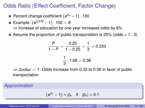
Percent change coefficient (eβk − 1) · 100
Example: (e0.079 − 1) · 100 = 8⇒ increase of education by one year increases odds by 8%
Assume the proportion of public transportation is 25% (odds = 1 : 3)
P1 − P
=0.25
1 − 0.25=
13
= 0.333
13· 1.08 = 0.36
⇒ ∆educ = 1: Odds increase from 0.33 to 0.36 in favor of publictransportation
Approximation
(eβk − 1) ≈ βk if |βk | < 0.1
Diekmann/Jann (ETH Zurich) Regression Models for Categorical Data ZA Spring Seminar 2008 72 / 188

Standardized Factor Change
To make effects comparable, it is sometimes sensible to weight themby the standard deviations of the X .
Standardized Factor Change
αskk = eβk ·sk
where
sk =
√√√1N
N∑i=1
(Xi − X)2
is the standard deviation of Xk
Interpretation: Effect of a standard deviation increase in X on theodds P/(1 − P)
The procedure makes not much sense for binary predictors, since inthis case the standard deviation has not much meaning.
Diekmann/Jann (ETH Zurich) Regression Models for Categorical Data ZA Spring Seminar 2008 73 / 188

Marginal/Partial EffectOdds may be more intuitive then Log-Odds, but what we really areinterested in are the effects on the probability P(Y = 1).Unfortunately P(Y = 1) is a non-linear function of X so that the effecton P(Y = 1) not only depends on the amount of change in X , butalso on the level of X at which the change occurs.
0
.25
.5
.75
1P
0 1 2 3 4 5x
A first step in the direction of interpreting effects on the probabilityscale is to compute the first derivative of the function at differentpositions.
Diekmann/Jann (ETH Zurich) Regression Models for Categorical Data ZA Spring Seminar 2008 74 / 188

Marginal/Partial Effect
In linear regression: ∂Y∂Xk
= βk
In logistic regression:
P =1
1 + e−[β0+β1X1+···+βmXm]=
11 + e−Z
=(1 + e−Z
)−1
∂P∂Xk
= −1
(1 + e−Z)2· (−βk )e−Z
= βk ·1
1 + e−Z︸ ︷︷ ︸P
·e−Z
1 + e−Z︸ ︷︷ ︸1−P
= βk · P(1 − P).
Marginal Effect in Logistic Regression∂P∂Xk
= βk · P(1 − P)
Diekmann/Jann (ETH Zurich) Regression Models for Categorical Data ZA Spring Seminar 2008 75 / 188

Marginal/Partial EffectMaximum marginal effect at P = 0.5 (the inflection point of theprobability curve)
βk ·12
(1 −
12
)= βk ·
14
Divide-by-four ruleThe maximum marginal effect of Xk is equal to βk/4.
0
.25
.5
.75
1P
X
Diekmann/Jann (ETH Zurich) Regression Models for Categorical Data ZA Spring Seminar 2008 76 / 188

Marginal/Partial Effect
Relative magnitudes of marginal effect for two variables
∂P/∂Xk
∂P/∂Xj=βk · P(1 − P)
βj · P(1 − P)=βk
βj
The ratio of coefficients reflects the relative magnitudes of themarginal effect on Pr(Y = 1).
Diekmann/Jann (ETH Zurich) Regression Models for Categorical Data ZA Spring Seminar 2008 77 / 188
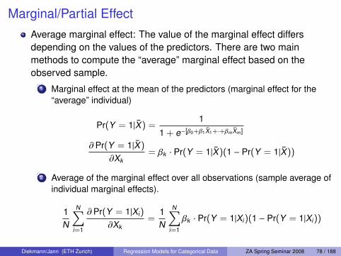
Marginal/Partial EffectAverage marginal effect: The value of the marginal effect differsdepending on the values of the predictors. There are two mainmethods to compute the “average” marginal effect based on theobserved sample.
1 Marginal effect at the mean of the predictors (marginal effect for the“average” individual)
Pr(Y = 1|X) =1
1 + e−[β0+β1X1+·+βmXm]
∂Pr(Y = 1|X)
∂Xk= βk · Pr(Y = 1|X)(1 − Pr(Y = 1|X))
2 Average of the marginal effect over all observations (sample average ofindividual marginal effects).
1N
N∑i=1
∂Pr(Y = 1|Xi)
∂Xk=
1N
N∑i=1
βk · Pr(Y = 1|Xi)(1 − Pr(Y = 1|Xi))
Diekmann/Jann (ETH Zurich) Regression Models for Categorical Data ZA Spring Seminar 2008 78 / 188

Marginal/Partial Effect
Marginal effect at the mean: Example
sex
0 1car 0 4 1
1 3 4
sex = 5/12 = 0.416
Pr(car = 1|sex) =1
1 + e−[−0.2876+1.6739·0.416]= 0.601
∂Pr(car = 1|sex)∂sex
= 1.6739 · 0.601(1 − 0.601) = 0.40
Diekmann/Jann (ETH Zurich) Regression Models for Categorical Data ZA Spring Seminar 2008 79 / 188

Marginal/Partial Effect: ProblemsMarginal effects at the mean of the predictors often do not makemuch sense. For binary variables, as in the example above, the meandoes not correspond to an observable value. In general, X may notbe a good description of the “typical” or “average” observation.Marginal effects are often only crude approximations of the “real”effects on the probability (especially for binary predictors).
.2.4
.6.8
1
P
0 1X
Diekmann/Jann (ETH Zurich) Regression Models for Categorical Data ZA Spring Seminar 2008 80 / 188

Elasticity
The elasticity, which is closely related to the marginal effect, can becomputed if the predictor has ratio scale level (metric variable with anatural zero-point).
Elasticity in logistic regression∂P/P∂Xk/Xk
=∂P∂Xk
Xk
P= βk Xk (1 − P)
Example: In traffic mode choice, let Xk be the price or travel duration.The elasticity can then (approximately) be interpreted as thepercent-percent effect⇒ percent change of P if Xk is increased byone percent.
Diekmann/Jann (ETH Zurich) Regression Models for Categorical Data ZA Spring Seminar 2008 81 / 188

Semi-Elasticity
Since P is on an absolute scale in the [0, 1] interval, thesemi-elasticity is usually better interpretable.
Semi-elasticity in logistic regression∂P∂Xk/Xk
=∂P∂Xk
Xk = βk Xk P(1 − P)
Interpretation: How much does P change (approximately) if Xk isincreased by one percent.
Example: If Xk is the price of a bus ticket and the semi-elasticity is−0.02, then the probability to use the bus decreases by twopercentage points if the price is increased by one percent.
Note: Similar to marginal effects, elasticities and semi-elasticitiesdepend on the values of the predictors in logistic regression.
Diekmann/Jann (ETH Zurich) Regression Models for Categorical Data ZA Spring Seminar 2008 82 / 188

PredictionsThe most direct approach to interpret the effects of the covariates onthe probability is to compute the predicted probabilities for differentsets of covariate values.
Prediction given vector Xi
Pi = Pr(Y = 1|Xi) =1
1 + e−[β0+β1Xi1+·+βmXim]
The predictions can then be reported in tables or in plots.Example: Predicted probability of driving a car depending on sex andage.
0.2
.4.6
.81
prob
abili
ty
2000 4000 6000 8000 10000income
malefemale
Diekmann/Jann (ETH Zurich) Regression Models for Categorical Data ZA Spring Seminar 2008 83 / 188

Discrete Change Effect
Based on predicted probabilities, the effect of a discrete change in anindependent variable, holding all other covariates constant, can becomputed.
Discrete Change Effect
∆ Pr(Y = 1|X)
∆Xk= Pr(Y = 1|X ,Xk + δ) − Pr(Y = 1|X ,Xk )
Unit change effect: Effect of a one unit change in Xk (Petersen 1985)
Unit Change Effect
∆ Pr(Y = 1|X)
∆Xk= Pr(Y = 1|X ,Xk + 1) − Pr(Y = 1|X ,Xk )
As outlined above, the partial change (marginal) effect does not equalthe unit change effect in the logit model.
Diekmann/Jann (ETH Zurich) Regression Models for Categorical Data ZA Spring Seminar 2008 84 / 188

Discrete Change Effect
Variants of discrete change effects
0-1 change (for binary covariates)
Pr(Y = 1|X ,Xk = 1) − Pr(Y = 1|X ,Xk = 0)
centered unit change
Pr(Y = 1|X , Xk + 0.5) − Pr(Y = 1|X , Xk − 0.5)
standard deviation change
Pr(Y = 1|X , Xk + 0.5sk ) − Pr(Y = 1|X , Xk − 0.5sk )
minimum-maximum change
Pr(Y = 1|X ,Xk = Xmaxk ) − Pr(Y = 1|X ,Xk = Xmin
k )
Diekmann/Jann (ETH Zurich) Regression Models for Categorical Data ZA Spring Seminar 2008 85 / 188

Discrete Change Effect
Simple example
Pr(car = 1|sex) =1
1 + e−[−0.2876+1.6739·sex]
sex = 0 : P0 =1
1 + e−[−0.2876]= 0.4286
sex = 1 : P1 =1
1 + e−[−0.2876+1.6739]= 0.80
⇒ ∆P = 0.80 − 0.4286 = 0.37
Diekmann/Jann (ETH Zurich) Regression Models for Categorical Data ZA Spring Seminar 2008 86 / 188

Discrete Change Effect
Values of the other covariates? ⇒ usually set to their mean
Pr(Y = 1|X ,Xk + δ) − Pr(Y = 1|X ,Xk )
In some cases, it might be more reasonable to use the median or themode for selected variables.
If the model contains categorical variables (e.g. sex), it can also beillustrative to compute separate sets of discrete change effects for thedifferent groups.
Furthermore, it can also be sensible to compute the “average”discrete change effect over the sample:
1N
N∑i=1
(Pr(Y = 1|Xi ,Xik + δ) − Pr(Y = 1|Xi ,Xik ))
Diekmann/Jann (ETH Zurich) Regression Models for Categorical Data ZA Spring Seminar 2008 87 / 188

Relative Risks
In cases where Pr(Y = 1) is very low (e.g. accident statistics), it canbe reasonable to express effects in terms of relative risks.
Example: Parachute Type A versus Type B
PA = 4 · 10−6, PB = 2 · 10−6
⇒ discrete change effect: PA − PB = 0.000002
⇒ relative risks: R = PA/PB = 2
(For fun see Smith and Pell, BMJ 2003, who complain about the lackof randomized controlled trials on parachute effectiveness.)
Diekmann/Jann (ETH Zurich) Regression Models for Categorical Data ZA Spring Seminar 2008 88 / 188

Part VI
Logistic Regression: Estimation
Maximum Likelihood Estimation
MLE for Linear Regression
MLE for Logit
Large Sample Properties of MLE
Summary
Diekmann/Jann (ETH Zurich) Regression Models for Categorical Data ZA Spring Seminar 2008 89 / 188

Maximum Likelihood Estimation (MLE)
Although it would be possible to use the (weighted nonlinear) leastsquares method, a Logit model is typically estimated by the maximumlikelihood method.
General estimation principle:
Least Squares (LS): minimize the squared deviations betweenobserved data and predictions
Maximum Likelihood (ML): maximize the likelihood (i.e. theprobability) of the observed data given the estimate
Diekmann/Jann (ETH Zurich) Regression Models for Categorical Data ZA Spring Seminar 2008 90 / 188

MLE – Example: Proportion of men
If π is the proportion of men in the population, then the probability ofhaving k men in a sample of size N is
Pr(k |π,N) =
(Nk
)πk (1 − π)N−k
(k follows a binomial distribution). Assumption: independent samplingwith identical probability (i.i.d.)
Assume k = 2 and N = 6. We can now ask: What value for π makesthis outcome most likely? The answer is found by maximizing thelikelihood function
L(π|k ,N) =
(Nk
)πk (1 − π)N−k
with respect to π. ⇒ Choose π so that the first derivative (gradient) iszero: ∂L(π|k ,N)/∂π = 0
Diekmann/Jann (ETH Zurich) Regression Models for Categorical Data ZA Spring Seminar 2008 91 / 188
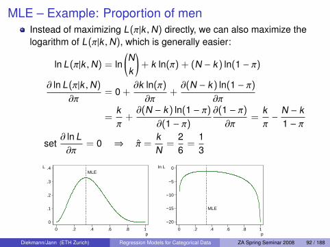
MLE – Example: Proportion of menInstead of maximizing L(π|k ,N) directly, we can also maximize thelogarithm of L(π|k ,N), which is generally easier:
ln L(π|k ,N) = ln(Nk
)+ k ln(π) + (N − k) ln(1 − π)
∂ ln L(π|k ,N)
∂π= 0 +
∂k ln(π)
∂π+∂(N − k) ln(1 − π)
∂π
=kπ
+∂(N − k) ln(1 − π)
∂(1 − π)∂(1 − π)∂π
=kπ−
N − k1 − π
set∂ ln L∂π
= 0 ⇒ π =kN
=26
=13
MLE
0
.1
.2
.3
.4L
0 .2 .4 .6 .8 1p
MLE
−20
−15
−10
−5
0ln L
0 .2 .4 .6 .8 1p
Diekmann/Jann (ETH Zurich) Regression Models for Categorical Data ZA Spring Seminar 2008 92 / 188

MLE for Linear RegressionModel:
Yi = β0 + β1Xi1 + · · ·+ βmXim + εi = X ′i β+ εi
εii.i.d∼ N(0, σ) ⇒ Yi
i.i.d∼ N(X ′i β, σ)
The probability density function for Yi is
f(Yi |X ′i β, σ) =1
σ√
2πe−
12σ2 (Yi−X ′i β)
2=
1σφ
(Yi − X ′i β
σ
)where φ(z) = 1√
2πe−z2/2 is the standard normal density, so that
L(β, σ|Y ,X) =N∏
i=1
1σφ
(Yi − X ′i β
σ
)The β that maximizes L also minimizes
∑(Yi − X ′i β)
2 ⇒ MLE = OLSin this case (but only if ε is assumed to be normally distributed)
Diekmann/Jann (ETH Zurich) Regression Models for Categorical Data ZA Spring Seminar 2008 93 / 188

MLE for Logit
Let Pi = Pr(Yi = 1) =(1 + e−(X
′i β)
)−1. The likelihood of a specific
observation can then be written as
Pr(Yi |Xi , β) = PYii (1 − Pi)
1−Yi =
Pi if Yi = 1
1 − Pi if Yi = 0
and the likelihood and log likelihood functions are
L(β|Y ,X) =N∏
i=1
PYii (1 − Pi)
1−Yi
ln L(β|Y ,X) =N∑
i=1
[Yi ln Pi + (1 − Yi) ln(1 − Pi)]
=N∑
i=1
YiX ′i β −N∑
i=1
ln(1 + eX ′i β
)Diekmann/Jann (ETH Zurich) Regression Models for Categorical Data ZA Spring Seminar 2008 94 / 188

MLE for Logit
Usually no closed form solution exists for the maximum of ln L so thatnumerical optimization methods are used (e.g. the Newton-Raphsonmethod). The general procedure is to start with an initial guess for theparameters and then iteratively improve on that guess untilapproximation is “good enough”.
Care has to be taken if the (log) likelihood function (surface) is notglobally concave, i.e. if local maxima exist.
Luckily, the Logit model has a globally concave log likelihood function,so that a single global maximum exists and the solution isindependent of the starting values.
Diekmann/Jann (ETH Zurich) Regression Models for Categorical Data ZA Spring Seminar 2008 95 / 188

Large Sample Properties of MLE
Consistency: asymptotically unbiased (expected value of MLEapproaches true value with increasing N)
Efficiency: asymptotically minimal sampling variance
Normality: estimates are asymptotically normally distributed (MLEare BAN, Best Asymtotic Normal estimator)⇒ statistical inference can be based on normal theory (e.g. Wald testfor single coefficients, likelihood ratio test for nested models)
(Fox 1997)
Diekmann/Jann (ETH Zurich) Regression Models for Categorical Data ZA Spring Seminar 2008 96 / 188

MLE: summary
Benefits of MLEvery flexible and can handle many kinds of models
desirable large sample properties
Drawbacks of MLEmay be biased and inefficient in small samples (MLE-Logit withN < 100 not recommended; depends on model complexity; see e.g.Peduzzi et al. 1996, Bagley et al. 2001)Example: MLE estimate of variance of x is 1/N
∑(xi − x)2, unbiased estimate is
1/(N − 1)∑
(xi − x)2
requires distributional assumptions
generally no closed form solutions (but computers do the job)
numerical algorithms may not converge in some cases (e.g. in Logit ifthere is perfect classification so that |β| → ∞)
Diekmann/Jann (ETH Zurich) Regression Models for Categorical Data ZA Spring Seminar 2008 97 / 188

Part VII
Logistic Regression: Inference
MLE and Statistical Inference
Significance Tests and Confidence Intervals
Likelihood Ratio Tests
Wald Test
Diekmann/Jann (ETH Zurich) Regression Models for Categorical Data ZA Spring Seminar 2008 98 / 188

MLE and Statistical InferenceMLE theory shows:
The sampling distribution of ML parameter estimates is asymptoticallynormal.
⇒ Therefore, statistical tests and confidence intervals can be basedon an estimate for the variance of the sampling distribution.
The variance-covariance matrix of an ML estimator for a parametervector θ is given as the negative of the inverse of the expected valueof the matrix of second derivatives of the log likelihood function.(The matrix of second derivatives of ln L(θ) is called the Hessian. Thenegative of the expectation of the Hessian is called the information matrix.)
Intuitive explanation: The second derivative indicates the curvature oflog likelihood function. If the function is flat, then there is muchuncertainty in the estimate. Variance reflects uncertainty.Cautionary note: Results are only asymptotic, large N required(N > 100)
Diekmann/Jann (ETH Zurich) Regression Models for Categorical Data ZA Spring Seminar 2008 99 / 188

MLE and Statistical Inference
Curvature of the log likelihood function and sample size:−
400
−30
0−
200
−10
00
ln L
−3 −2 −1 0 1b_0
N = 100
−10
00−
900
−80
0−
700
−60
0ln
L
−3 −2 −1 0 1b_0
N = 1000
Model: Pr(Y = 1) = 11+e−β0
Diekmann/Jann (ETH Zurich) Regression Models for Categorical Data ZA Spring Seminar 2008 100 / 188

MLE and Statistical InferenceExample: Logit model with only a constant β0, i.e. π = Pr(Y = 1) is aconstant.
MLE of π: π = kN , where k is the observed number of events
What are the variance and standard deviation (= standard error) ofthe sampling distribution of π?
L(π|k ,N) =
(Nk
)πk (1 − π)N−k
ln L(π|k ,N) = ln(Nk
)+ k ln(π) + (N − k) ln(1 − π)
ln L ′ =∂ ln L∂π
=kπ−
N − k1 − π
= kπ−1 − (N − k)(1 − π)−1 ⇒ π =kN
ln L ′′ =∂2 ln L∂π2 = −kπ−2 − (N − k)(1 − π)−2 = −
[kπ2 +
N − k(1 − π)2
]Note: ln L ′′ < 0 for all π (concave), i.e. ln L(π) is maximum.Diekmann/Jann (ETH Zurich) Regression Models for Categorical Data ZA Spring Seminar 2008 101 / 188

MLE and Statistical Inference
ln L ′′ = −[
kπ2 +
N − k(1 − π)2
]= −
(1 − π)2k + p2(N − k)
π2(1 − π)2 ·NN
= −π2 − 2π k
N + kN
1Nπ
2(1 − π)2
E[k/N] = π
E[ln L ′′] = −π2 − 2π2 + π1Nπ
2(1 − π)2= −
π − π2
1Nπ
2(1 − π)2= −
π(1 − π)1Nπ
2(1 − π)2
= −1
1Nπ(1 − π)
Diekmann/Jann (ETH Zurich) Regression Models for Categorical Data ZA Spring Seminar 2008 102 / 188
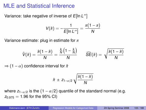
MLE and Statistical Inference
Variance: take negative of inverse of E[ln L ′′]
V(π) = −1
E[ln L ′′]=π(1 − π)
N
Variance estimate: plug in estimate for π
V(π) =π(1 − π)
N=
kN
(1 − k
N
)N
SE(π) =
√π(1 − π)
N
⇒ (1 − α) confidence interval for π
π ± z1−α/2
√π(1 − π)
N
where z1−α/2 is the (1 − α/2) quantile of the standard normal (e.g.z0.975 = 1.96 for the 95% CI)
Diekmann/Jann (ETH Zurich) Regression Models for Categorical Data ZA Spring Seminar 2008 103 / 188

MLE and Statistical Inference
In general for β = [β1, β2, . . . , βm]T
Hessian
H =∂2 ln L∂β2 =
∂2 ln L∂β1∂β1
∂2 ln L∂β1∂β2
· · · ∂2 ln L∂β1∂βm
......
. . ....
∂2 ln L∂βm∂β1
∂2 ln L∂βm∂β2
· · · ∂2 ln L∂βm∂βm
MLE Variance-Covariance Matrix
V(β) =
V(β1) V(β1, β2) · · · V(β1, βm)...
.... . .
...
V(βm, β1) V(βm, β2) · · · V(βm)
= −1
E[H]
Diekmann/Jann (ETH Zurich) Regression Models for Categorical Data ZA Spring Seminar 2008 104 / 188

Significance Test for a Single Regressor
According to ML theory, parameter estimate βk is asymptoticallynormal, i.e.
βka∼ N(βk ,V(βk ))
Using the variance estimate V(βk ) we can therefore construct asignificance test for βk in the usual way.
Let the null hypothesis be H0 : βk = β0k . The test statistic then is
Z =βk − β
0k
SE(βk )with SE(βk ) =
√V(βk )
(SE = standard error).
The null hypothesis is rejected on significance level α if |Z | > z1−α/2
where z1−α/2 is the (1 − α/2)-quantile of the standard normaldistribution.
Diekmann/Jann (ETH Zurich) Regression Models for Categorical Data ZA Spring Seminar 2008 105 / 188

Significance Test for a Single RegressorUsually: Test against zero on a 5% level
H0 : βk = 0 (i.e. β0k = 0)
5% significance level (α = 0.05)
Test statistic: Z =βk
SE(βk )
a∼ N(0, 1)
reject H0 if |Z | > 1.96
alpha/2 = 0.025(reject H0)
alpha/2 = 0.025(reject H0)
f(z)
−1.96 0 1.96z
Diekmann/Jann (ETH Zurich) Regression Models for Categorical Data ZA Spring Seminar 2008 106 / 188

Confidence Interval for a Single Regressor
(1 − α)-Confidence Interval
βk ± z1−α/2 · SE(βk )
Usually: 95%-Confidence Interval[βk − 1.96 · SE(βk ) , βk + 1.96 · SE(βk )
]
Diekmann/Jann (ETH Zurich) Regression Models for Categorical Data ZA Spring Seminar 2008 107 / 188
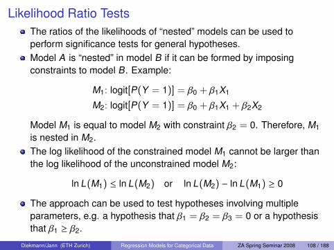
Likelihood Ratio TestsThe ratios of the likelihoods of “nested” models can be used toperform significance tests for general hypotheses.Model A is “nested” in model B if it can be formed by imposingconstraints to model B. Example:
M1: logit[P(Y = 1)] = β0 + β1X1
M2: logit[P(Y = 1)] = β0 + β1X1 + β2X2
Model M1 is equal to model M2 with constraint β2 = 0. Therefore, M1
is nested in M2.The log likelihood of the constrained model M1 cannot be larger thanthe log likelihood of the unconstrained model M2:
ln L(M1) ≤ ln L(M2) or ln L(M2) − ln L(M1) ≥ 0
The approach can be used to test hypotheses involving multipleparameters, e.g. a hypothesis that β1 = β2 = β3 = 0 or a hypothesisthat β1 ≥ β2.
Diekmann/Jann (ETH Zurich) Regression Models for Categorical Data ZA Spring Seminar 2008 108 / 188

Likelihood Ratio Tests
Likelihood Ratio TestGeneral result: The likelihood ratio statistic
LR = G2 = −2 ln(L(MC)
L(MU)
)= 2 ln L(MU) − 2 ln L(MC)
where MC is the constrained (restricted, nested, null) model and MU is theunconstrained (full) model, is asymptotically chi-square distributed withdegrees of freedom equal to the number of independent constraints.
Example applications:I overall LR test of the full modelI LR test of a single coefficientI LR test of a subset of coefficientsI LR test of equality of two coefficients
Diekmann/Jann (ETH Zurich) Regression Models for Categorical Data ZA Spring Seminar 2008 109 / 188

Overall LR Test of Full Model
Is the model significant at all? Does the model “explain” anything?
Null hypothesis:H0: β1 = β2 = · · · = βm = 0
Models:
MC : logit[P(Y = 1)] = β0
MU: logit[P(Y = 1)] = β0 + β1X1 + β2X2 + · · ·+ βmXm
Test statistic:
LR = 2 ln L(MU) − 2 ln L(MC)a∼ χ2(m)
Reject H0 at the α level if LR > χ21−α(m)
[Note: The log likelihood of the null model in this case isln L(MC) = ln
(Nk
)+ k ln(k/N) + (N − k) ln(1 − k/N).]
Diekmann/Jann (ETH Zurich) Regression Models for Categorical Data ZA Spring Seminar 2008 110 / 188

LR Test of a Single Coefficient
Is coefficient βk significant?
Null hypothesis:H0: βk = 0
Models:
MC : Z = β0 + · · ·+ βk−1Xk−1 + βk+1Xk+1 · · ·+ βmXm
MU: Z = β0 + · · ·+ βk−1Xk−1 + βk Xk + βk+1Xk+1 · · ·+ βmXm
Test statistic:
LR = 2 ln L(MU) − 2 ln L(MC)a∼ χ2(1)
Reject H0 at the α level if LR > χ21−α(1)
The LR test of a single coefficient is asymptotically equivalent to the testbased on the Hessian discussed above.
Diekmann/Jann (ETH Zurich) Regression Models for Categorical Data ZA Spring Seminar 2008 111 / 188

LR Test of a Subset Of CoefficientsIs any coefficient in a set of coefficients different from zero? Does the setof coefficients jointly “explain” anything?
Note: This is different than testing each parameter separately!
Null hypothesis:H0: βk = · · · = βl = 0
Models:
MC : Z = β0 + · · ·+ · · ·+ βmXm
MU: Z = β0 + · · ·+ βk Xk + · · ·+ βlXl + · · ·+ βmXm
Test statistic:
LR = 2 ln L(MU) − 2 ln L(MC)a∼ χ2(l − k + 1)
Reject H0 at the α level if LR > χ21−α(l − k + 1)
Diekmann/Jann (ETH Zurich) Regression Models for Categorical Data ZA Spring Seminar 2008 112 / 188
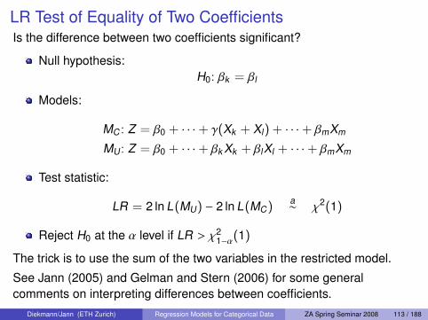
LR Test of Equality of Two CoefficientsIs the difference between two coefficients significant?
Null hypothesis:H0: βk = βl
Models:
MC : Z = β0 + · · ·+ γ(Xk + Xl) + · · ·+ βmXm
MU: Z = β0 + · · ·+ βk Xk + βlXl + · · ·+ βmXm
Test statistic:
LR = 2 ln L(MU) − 2 ln L(MC)a∼ χ2(1)
Reject H0 at the α level if LR > χ21−α(1)
The trick is to use the sum of the two variables in the restricted model.
See Jann (2005) and Gelman and Stern (2006) for some generalcomments on interpreting differences between coefficients.
Diekmann/Jann (ETH Zurich) Regression Models for Categorical Data ZA Spring Seminar 2008 113 / 188

Wald TestAn alternative, asymptotically equivalent approach to testing thedifference between nested models is the Wald test, which is based onthe variance-covariance matrix of the estimates.Example: For the test of the null hypothesis that β1 is equal to β2, theWald statistic is
W =(β1 − β2)
2
V(β1) + V(β2) + Cov(β1, β2)
a∼ χ2(1)
See, e.g., Long (1997: 89pp.) for the general form of the test andfurther details. The Wald test is analogous to the generalized F-test inlinear regression (Greene 2003:95pp.).The advantage of the Wald test over the LR test is that only the fullmodel has to be estimated.Some people prefer the LR test over the Wald test (especially inmoderate samples) because there is (weak) evidence that it is moreefficient and behaves less erratic. But note that both procedures canbe quite off in small samples.
Diekmann/Jann (ETH Zurich) Regression Models for Categorical Data ZA Spring Seminar 2008 114 / 188

Relation between LR test and Wald test
LR test: Difference between ln L(β) and ln L(β0)
Wald test: Difference between β and β0 weighted by curvature of loglikelihood, ∂2 ln L/∂β2
(Fox 1997)
Diekmann/Jann (ETH Zurich) Regression Models for Categorical Data ZA Spring Seminar 2008 115 / 188

Significance Test of a Single Regressor in SPSS
SPSS reports a Wald statistic with one degree of freedom for theindividual tests of the single regressors.
The Wald statistic is equivalent to the square of Z of the usualsignificance test discussed above in this case.
W =
βk
SE(βk )
2a∼ χ2(1)
Reject H0: βk = 0 if W is larger than the (1 − α) quantile of thechi-squared distribution with 1 degree of freedom.
Note: The square of a standard normally distributed variable ischi-square distributed with 1 degree of freedom.
Diekmann/Jann (ETH Zurich) Regression Models for Categorical Data ZA Spring Seminar 2008 116 / 188

Part VIII
Logistic Regression: Diagnostics and Goodness-of-Fit
Pearson Chi-Square and Deviance
Residuals and Influence
Classification Table
Goodness-of-Fit Measures
Diekmann/Jann (ETH Zurich) Regression Models for Categorical Data ZA Spring Seminar 2008 117 / 188

Pearson Chi-Square and Deviance
Two concepts to measure discrepancy between model and dataI Pearson statistic: difference between observed data and predicted
probabilitiesI Deviance: difference between the likelihood of a “saturated” model
(= perfect model) and the likelihood of the fitted model
To formalize the concepts it is useful to think in “covariate patterns”(distinct patterns of values in X) rather then observations.Notation
I J: number of covariate patternsI if some observations have the same X values, then J < NI if each observation has its own unique covariate pattern, then J = NI Xj : jth covariate pattern, j = 1, . . . , JI nj : number of observations with covariate values equal to XjI Yj : the mean of Y (proportion of ones) among the observations with
with covariate pattern Xj
Diekmann/Jann (ETH Zurich) Regression Models for Categorical Data ZA Spring Seminar 2008 118 / 188

Pearson Chi-Square and Deviance
Pearson X2
Difference between observed proportions Yj and predictedprobabilities πj = (1 + e−X ′j β)−1
Ej = Yj − πj , Yj ∈ [0, 1], πj ∈ [0, 1]⇒ Ej ∈ [−1, 1]
Pearson statistic
X2 =J∑
j=1
r2j , rj =
√nj
Yj − πj√πj(1 − πj)
Interpretation: Sum of variance weighted residuals
rj is called the “Pearson residual”
If J = N: X2 =∑N
i=1 r2i , ri = (Yi − πi)
/√πi(1 − πi)
Diekmann/Jann (ETH Zurich) Regression Models for Categorical Data ZA Spring Seminar 2008 119 / 188

Pearson Chi-Square and DevianceDeviance
Discrepancy between the log likelihood L(β) of the estimated modeland the log likelihood LS of a “saturated” model (i.e. a model with oneparameter per covariate pattern)
Deviance
D = −2 lnL(β)
LS
= 2[ln LS − ln L(β)]
Since ln LS =∑
j nj[Yj ln(Yj) + (1 − Yj) ln(1 − Yj)]
ln L(β) =∑
j nj[Yj ln(πj) + (1 − Yj) ln(1 − πj)]
D =J∑
j=1
d2j , dj = ±
√2nj
[Yj ln
(Yj
πj
)+ (1 − Yj) ln
(1 − Yj
1 − πj
)]where sign of the deviance residual dj agrees with the sign of Yj − πj
Diekmann/Jann (ETH Zurich) Regression Models for Categorical Data ZA Spring Seminar 2008 120 / 188

Pearson Chi-Square and Deviance
Deviance
If J = N:
D = −2 ln L(β) =N∑
i=1
d2i
withdi = ±
√−2 [Yi ln(πi) + (1 − Yi) ln(1 − πi)]
since
ln Ls =N∑
i=1
[Yi ln(Yi) + (1 − Yi) ln(1 − Yi)] = 0
.
Diekmann/Jann (ETH Zurich) Regression Models for Categorical Data ZA Spring Seminar 2008 121 / 188

Pearson Chi-Square and DevianceOverall goodness-of-fit test:
Large values for X2 or D provide evidence against the null hypothesisthat the model fits the observed data.
Think of a J × 2 table with distinct covariate patterns in the rows andthe values of Y (0 and 1) in the columns. X2 and D are the Pearsonstatistic and the likelihood ratio statistic for the test of the differencebetween the observed cell frequencies and the expected cellfrequencies using the fitted model.
The null hypothesis is rejected if X2 > χ21−α(J −m − 1) or
D > χ21−α(J −m − 1), respectively, where m is the number of
regressors in the model.
However, the test is only valid in a design with many observations percovariate pattern. For example, if the model contains continuousregressors, J will increase with N and the cell counts remain small.As a consequence, X2 and D are not asymptotically chi-squaredistributed.
Diekmann/Jann (ETH Zurich) Regression Models for Categorical Data ZA Spring Seminar 2008 122 / 188

Pearson Chi-Square and Deviance
Hosmer-Lemeshow test
To avoid the problem of growing J with increasing N, Hosmer andLemeshow proposed a test based on grouped data (1980; Lemeshowand Hosmer 1982)
I The data are divided into g (approx.) equally sized groups based onpercentiles of the predicted probabilities (⇒ g × 2 table)
I In each group the expected and observed frequencies are computedfor Y = 0 and Y = 1.
I A Pearson X2 statistic is computed from these cell frequencies in theusual manner.
I The null hypothesis is rejected if the statistic exceeds the(1 − α)-quantile of the χ2 distribution with g − 2 degrees of freedom.
For alternative approaches see the discussion in Hosmer andLemeshow (2000: 147pp.).
Diekmann/Jann (ETH Zurich) Regression Models for Categorical Data ZA Spring Seminar 2008 123 / 188

Residuals and InfluenceA goal of regression diagnostics is to evaluate whether there aresingle observations that badly fit the model and exert large influenceon the estimate (see, e.g., Fox 1991, Jann 2006). We have lessconfidence in estimates if they strongly depend on only a fewinfluential cases.
I Outliers: Observations for which the difference between the modelprediction and the observed value is large.
I Influence: The effect of an individual observation (or a group ofobservations) on the estimate.
A popular measure is Cook’s Distance as an overall measure for theinfluence of an observation on the estimated parameter vector.
Outliers or influential observations can be due to data errors. But theycan also be a sign of model misspecification.
The regression diagnostics tools, which were developed for linearregression, can be translated to logistic regression (Pregibon 1981;good discussion in Hosmer and Lemeshow 2000).
Diekmann/Jann (ETH Zurich) Regression Models for Categorical Data ZA Spring Seminar 2008 124 / 188

Residuals and Influence[For simplicity, assume J = N for the following discussion.]
As noted before, if Y is a binary variable, the difference between Yi
and πi = Pr(Yi = 1) is heteroscedastic:
V(Yi |Xi) = V(Yi − πi) = πi(1 − πi)
This suggests using the Pearson residual
ri =Yi − πi√πi(1 − πi)
as a standardized measure for the discrepancy between anobservation and the model prediction.
However, because πi is an estimate and the observed Yi hasinfluence on that estimate, V(Yi − πi) , πi(1 − πi) so that the varianceof ri is not 1 and the residuals from different observations cannot becompared.
Diekmann/Jann (ETH Zurich) Regression Models for Categorical Data ZA Spring Seminar 2008 125 / 188

Residuals and InfluenceAn improved measure is the standardized Pearson residual
rSi =
ri√
1 − hii
where hii = πi(1 − πi)X ′i V(β)Xi
rSi has variance 1 and can be compared across observations. A large
value of rSi indicates bad fit for observation i.
hii is called the leverage or hat value and is a measure for thepotential influence of an observation on the estimate. The leveragemainly depends on how “atypical” an observation’s X values are.
(a)
y1
x10 10 20 30
0
10
20
30(b)
y2
x10 10 20 30
0
10
20
30
Diekmann/Jann (ETH Zurich) Regression Models for Categorical Data ZA Spring Seminar 2008 126 / 188

Residuals and InfluenceObservations with a large residual and a large leverage exert stronginfluence on the model estimate.A measure to summarize this influence is Cook’s Distance
∆βi =r2i hii
(1 − hii)2 =(rS
i )2hii
1 − hii
Other popular measures are the influence on the Pearson chi-squarestatistic or the Deviance:
∆X2i =
r2i
1 − hii= (rS
i )2 ∆Di ≈d2
i
1 − hii
Large values indicate strong influence.Problematic observations can be easily spotted using index plots of,say, ∆βi . Another popular graph is to plot the statistic against thepredicted probabilities and use different colors/symbols for Yi = 0 andYi = 1.
Diekmann/Jann (ETH Zurich) Regression Models for Categorical Data ZA Spring Seminar 2008 127 / 188

Residuals and Influence: Example
“Did you ever cheat on your partner?” by age, sex, etc.
Model estimates:
. logit cheat male age highschool extraversion cheat_ok, nolog
Logistic regression Number of obs = 566LR chi2(5) = 44.33Prob > chi2 = 0.0000
Log likelihood = -294.4563 Pseudo R2 = 0.0700
cheat Coef. Std. Err. z P>|z| [95% Conf. Interval]
male -.0289207 .2194078 -0.13 0.895 -.4589521 .4011108age .0303383 .0075396 4.02 0.000 .015561 .0451155
highschool -.1937281 .2138283 -0.91 0.365 -.6128239 .2253677extraversion .2514374 .0835575 3.01 0.003 .0876676 .4152072
cheat_ok .2733903 .0739183 3.70 0.000 .128513 .4182675_cons -3.793885 .5430144 -6.99 0.000 -4.858174 -2.729597
Diekmann/Jann (ETH Zurich) Regression Models for Categorical Data ZA Spring Seminar 2008 128 / 188

Residuals and Influence: Example
Index plot of ∆β
379
456
0.0
5.1
.15
.2.2
5P
regi
bon’
s db
eta
0 200 400 600off
Diekmann/Jann (ETH Zurich) Regression Models for Categorical Data ZA Spring Seminar 2008 129 / 188

Residuals and Influence: Example
Plot of ∆β by prediction
379
456
0.0
5.1
.15
.2.2
5P
regi
bon’
s db
eta
0 .2 .4 .6 .8
Diekmann/Jann (ETH Zurich) Regression Models for Categorical Data ZA Spring Seminar 2008 130 / 188

Residuals and Influence: Example
List problematic observations:
. list dbeta cheat male age highschool extraversion cheat_ok if dbeta>.1
dbeta cheat male age highsc˜l extrav˜n cheat_ok
379. .1088898 0 0 53.70551 0 6.666667 6456. .2271219 0 0 107 1 4.333333 3
Observation 379 seems to be okay although somewhat atypical.However, there appears to be a data error in observation 456(age > 100). The data are from an online survey and respondentshad to pick their birth year from a dropdown list. Value 0 was stored ifthe respondent did not make a selection. These invalid observationswere accidently included when computing the age variable.
Diekmann/Jann (ETH Zurich) Regression Models for Categorical Data ZA Spring Seminar 2008 131 / 188

What to do about outliers/influential data?
Take a close look at the data.
Correct, or possibly exclude, erroneous data (only in clear-cut cases).
Compare models in which the outliers are included with models inwhich they are excluded. If the main results do not change you’re onthe save side.
Think about the outliers and improve your model/theory because . . .An apparently wild (or otherwise anomalous) observation isa signal that says: “Here is something from which we maylearn a lesson, perhaps of a kind not anticipatedbeforehand, and perhaps more important than the mainobject of the study.” (Kruskal 1960)
Diekmann/Jann (ETH Zurich) Regression Models for Categorical Data ZA Spring Seminar 2008 132 / 188

Goodness-of-Fit: Classification TableOverall goodness-of-fit: How well does the estimated model describethe observed data?One way to asses the goodness-of-fit is to compare the observeddata with the “maximum probability rule” predictions
Yi =
0 if πi ≤ 0.5
1 if πi > 0.5
Classification table: Table summarizing the number of “true” and“false” predictions
predicted
0 1
observed 0 true false
1 false true
Problem: Prediction table not very useful for extreme distributions (i.e.if Y is close to 0 or 1).
Diekmann/Jann (ETH Zurich) Regression Models for Categorical Data ZA Spring Seminar 2008 133 / 188

Classification Table: ExampleExample (H = 169): predicted
0 1
observed 0 25 47
1 15 82
Percentage of true predictions using the model:
25 + 82169
= 0.63 = 63%
However: Unconditional prediction (i.e. predict modal category for allobservations, here: Y = 1) yields
15 + 82169
= 0.57 = 57%
⇒ model improves proportion of true predictions by 6 percentagepoints.
Diekmann/Jann (ETH Zurich) Regression Models for Categorical Data ZA Spring Seminar 2008 134 / 188

Goodness-of-Fit Measures
It may be desirable to summarize the overall goodness-of-fit of amodel using a single number.
In linear regression this is done by the R-squared.
A number of fit measures imitating the R-squared have beendeveloped for logistic regression (and other models).
Critique: Scalar measures of fit should always be interpreted incontext. How high the value of such a measure should be for themodel to be a “good” model strongly depends on the research topicand the nature of the data.
Diekmann/Jann (ETH Zurich) Regression Models for Categorical Data ZA Spring Seminar 2008 135 / 188

Goodness-of-Fit Measures: R2 in Linear Regression
Various interpretations are possible for the R-squared, but incomparison to linear regression these interpretations lead to differentmeasures in logistic regression. Two of the interpretations are:
I Proportion of explained variation in Y
R2 =
∑(Yi − Y)2∑(Yi − Y)2
= 1 −∑
(Yi − Yi)2∑
(Yi − Y)2
I Transformation of the likelihood ratio (assumption: ε ∼ N(0, σ); L0 isthe likelihood of a model with just the constant)
R2 = 1 − (L0/L)2/N
R2 ∈ [0, 1], with higher values indicating better fit.
Diekmann/Jann (ETH Zurich) Regression Models for Categorical Data ZA Spring Seminar 2008 136 / 188

Goodness-of-Fit Measures: Pseudo-R2
R2 measures can be constructed for logistic regression (or othermodels) by analogy to one of the interpretations of R2 in linearregression.
These measures are called pseudo-R-squared.Some desirable properties:
I normalized to [0, 1]I clear interpretation of values other than 0 and 1
Diekmann/Jann (ETH Zurich) Regression Models for Categorical Data ZA Spring Seminar 2008 137 / 188

Pseudo-R2: Explained Variation
Efron’s pseudo-R2: explained variation based on predictedprobabilities
R2Efron = 1 −
∑ni=1(Yi − πi)
2∑ni=1(Yi − Y)2
∈ [0, 1]
In the case where J, the number of distinct covariate patterns, issmaller then N, the statistic should be computed as (see Hosmer andLemeshow 2001:165)
R2SSC = 1 −
∑Jj=1[nj(Yj − πj)]
2∑Jj=1[nj(Yj − Y)]2
where nj is the number of observations with covariate pattern Xj andYj is the mean of Y among these observations.
Diekmann/Jann (ETH Zurich) Regression Models for Categorical Data ZA Spring Seminar 2008 138 / 188
Pseudo-R2: Explained Variation
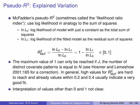
McFadden’s pseudo-R2 (sometimes called the “likelihood ratioindex”): use log likelihood in analogy to the sum of squares
I ln L0: log likelihood of model with just a constant as the total sum ofsquares
I ln L1: log likelihood of the fitted model as the residual sum of squares
R2McF =
ln L0 − ln L1
ln L0= 1 −
ln L1
ln L0∈ [0, 1]
The maximum value of 1 can only be reached if J, the number ofdistinct covariate patterns is equal to N (see Hosmer and Lemeshow2001:165 for a correction). In general, high values for R2
McF are hardto reach and already values within 0.2 and 0.4 usually indicate a verygood fit.
Interpretation of values other than 0 and 1 not clear.
Diekmann/Jann (ETH Zurich) Regression Models for Categorical Data ZA Spring Seminar 2008 139 / 188

Pseudo-R2: Explained Variation
McFadden’s pseudo-R2 increases if variables are added to themodel. A proposed correction is
R2McF = 1 −
ln L1 −mln L0
where m is the number regressors. If adding variables to a model,R2
McF will only increase if the log likelihood increases by more than 1for each added variable.
R2McF can be used to compare models (if they are based on the same
set of observations)
Diekmann/Jann (ETH Zurich) Regression Models for Categorical Data ZA Spring Seminar 2008 140 / 188

Pseudo-R2: Transformation of Likelihood Ratio
Maximum likelihood pseudo-R2 / Cox and Snell’s pseudo-R2
R2ML = 1 −
(L0
L1
)2/N
= 1 − e−LR/N
where LR is the likelihood ratio chi-square statistic.
Cragg and Uhler pseudo-R2 / Nagelkerke pseudo-R2: The maximumof R2
ML is 1 − (L0)2/N. This suggests the following correction
R2N =
R2ML
1 − (L0)2/N
so that the measure can take on values between 0 and 1.
Diekmann/Jann (ETH Zurich) Regression Models for Categorical Data ZA Spring Seminar 2008 141 / 188

Predictive Pseudo-R2 based on Classification Table
The information can in the classification table (see above) can beused to construct a R2 that reflects the prediction errors according tothe “maximum probability rule”
Let Yi = 0 if πi ≤ 0.5 and Yi = 1 if πi > 0.5, then
R2Count =
#(Yi = Yi)
N
Even without explanatory variables (i.e. if we use the mode ofoutcome categories as prediction for all observations) R2
Count is atleast 50%.
Diekmann/Jann (ETH Zurich) Regression Models for Categorical Data ZA Spring Seminar 2008 142 / 188

Predictive Pseudo-R2 based on Classification Table
Let M = max[#(Y = 0),#(Y = 1)], then
R2Count =
#(Yi = Yi) −MN −M
R2Count has a PRE interpretation (Proportional Reduction in Error). It
indicates the proportional reduction in prediction errors compared to amodel with only a constant.
Problem: R2Count is not very sensitive and is often 0 (especially if
Pr(Y = 1) is generally close to 0 or 1).
Diekmann/Jann (ETH Zurich) Regression Models for Categorical Data ZA Spring Seminar 2008 143 / 188

Information Measures
Akaike Information Criterion (AIC) and Bayesian Information Criterion(BIC)
AIC =−2 ln L(β) + p
N
BIC = −2 ln L(β) + p ln(N)
where p is the number of parameters in the model
General interpretation: the smaller AIC or BIC, the better the model fit
AIC and BIC can be used to compare models (also non-nestedmodels). The model with the smaller AIC or BIC is preferred.
Interpretation of BIC differences (strength of evidence favoring themodel with the smaller BIC): 0-2 weak, 2-6 positive, 6-10 strong, > 10very strong
Diekmann/Jann (ETH Zurich) Regression Models for Categorical Data ZA Spring Seminar 2008 144 / 188

Part IX
Logistic Regression: Specification
Specification Error
Excursus: Categorical Predictors
Nonlinearity
Non-Additivity and Interaction Effects
Numerical Problems: Zero Cells, Complete Separation, Collinearity
Diekmann/Jann (ETH Zurich) Regression Models for Categorical Data ZA Spring Seminar 2008 145 / 188

Specification Error
Assuming the Logit model is essentially correct, i.e. that the modelhas the general form logit[Pr(Y = 1)] = Xβ, we can still misspecifythe right hand side (RHS) of the equation.
Some specification errors are:I Omitted variables: Hard to detect with statistical approaches since
this is more of a theoretical issue. If an important variable Z that affectsboth Y and X is missing in the model, then the estimate of the effect ofX on Y will be biased (since it also contains the “indirect” effect of Z onY through X ).
I Nonlinearity: The effect of X on logit[Pr(Y = 1)] might be nonlinear.This is also a theoretical issues to some degree, but departures fromlinearity can be detected statistically. General procedure: Model theeffect nonlinearly and compare the results.
I Non-additivity: Assume the model contains X1 and X2. The effect ofX1 is assumed to be independent of the value of X2. This might not betrue. Non-additive model can be constructed using interaction terms.
Diekmann/Jann (ETH Zurich) Regression Models for Categorical Data ZA Spring Seminar 2008 146 / 188

Excursus: Categorical Predictors
Binary categorical variables (e.g. sex) can be included in a Logitmodel without problem. The effect measures the difference in the logodds between the two groups defined by the variable.
What to do if an independent variable X is categorical and has morethan two categories (e.g. religious denomination)? We cannot justinclude the variable in the model because the parameter estimatewould arbitrary (e.g. a change in the distances between the codes forthe categories, which would not change the meaning of the variable,would change yield a different parameter estimate).
The solution is to divide the variable into separate indicator variables,one for each category.
Diekmann/Jann (ETH Zurich) Regression Models for Categorical Data ZA Spring Seminar 2008 147 / 188
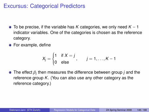
Excursus: Categorical Predictors
To be precise, if the variable has K categories, we only need K − 1indicator variables. One of the categories is chosen as the referencecategory.
For example, define
Xj =
1 if X = j
0 else, j = 1, . . . ,K − 1
The effect βj then measures the difference between group j and thereference group K . (You can also use any other category as thereference category.)
Diekmann/Jann (ETH Zurich) Regression Models for Categorical Data ZA Spring Seminar 2008 148 / 188

Excursus: Categorical Predictors
The coding above is called the dummy or indicator coding. Othercoding schemes can be used. Two examples are given bellow.
Effect coding: deviation from “grand mean” (the effect for thereference category is the negative of the sum of the effects for theother categories)
Xj =
1 if X = j
−1 if X = k
0 else
, j = 1, . . . ,K − 1
Split coding for ordinal variables: the parameters represent thedifferences form one category to the next
Xj =
1 if X ≥ j
0 else, j = 2, . . . ,K
Diekmann/Jann (ETH Zurich) Regression Models for Categorical Data ZA Spring Seminar 2008 149 / 188

Nonlinear Effects
The effect of a variable X on the log odds may be nonlinear.
Some strategies to model nonlinear effects:I categorize the variable and use dummies (or splines); very flexible,
however, choice of categories is arbitraryI if a variable is discrete and has only few values, the most flexible way to
model the effect is to use separate dummies for the valuesI polynomials (quite flexible, but bad for extrapolation)I nonlinear transformations of variablesI combinations of the above
For data exploration, i.e. as a first check for nonlinearity,“non-parametric” approaches may be useful. For example, it is oftenhelpful to visualize relationships using scatterplot smoothers such asthe the Lowess (see Fox 2000 for an overview).
Diekmann/Jann (ETH Zurich) Regression Models for Categorical Data ZA Spring Seminar 2008 150 / 188

Nonlinear Effects: Polynomials
A nonlinear relationship can be modeled by adding powers of X to theequation
logit[Pr(Y = 1)] = β0 + β1X + β2X2 + β3X3 + . . .
Most common is the quadratic model model⇒ parabolic effect(higher order models are usually hard to interpret)
log
odds
0 2 4 6 8 10x
b1 > 0, b2 < 0
log
odds
0 2 4 6 8 10x
b1 < 0, b2 > 0
Diekmann/Jann (ETH Zurich) Regression Models for Categorical Data ZA Spring Seminar 2008 151 / 188

Nonlinear Effects: Transformations
Example: take the logarithm of X
logit[Pr(Y = 1)] = β0 + β1 ln(X)
log
odds
0 2 4 6 8 10x
b > 0
log
odds
0 2 4 6 8 10x
b < 0
Interpretation: Effect of proportional change in XI If X is increased by one percent, then the log odds change by approx.β/100 (to be precise: β · ln(1.01))
I Odds ratio: a one percent increase in X changes the odds by approx.β1 percent (the odds ratio is 1.01β)⇒ elasticity
Diekmann/Jann (ETH Zurich) Regression Models for Categorical Data ZA Spring Seminar 2008 152 / 188

Non-Additivity and Interaction Effects
The effect of a variable X1 may depend on the value of anothervariable X2. Think of the effect of getting married on the probability tobe in the labor force. Probably the effect is different for men andwomen.
Non-additivity: This means that if X1 and X2 change simultaneously,then the effect of this simultaneous change is not simply the sum ofthe two separate effects.
Non-additive models can be fitted by including products of variables(“interaction terms”):
logit[P(Y = 1)] = β0 + β1X1 + β2X2 + β3X1X2
For example, the effect of X1 in this model is β1 + β3X3
When computing results such as marginal effects or discrete changeeffects, these dependencies have to be taken into account.
Diekmann/Jann (ETH Zurich) Regression Models for Categorical Data ZA Spring Seminar 2008 153 / 188

Zero Cells
For categorical covariates there is sometimes no variation in Y forone of the groups. The Logit model does not converge in this casebecause |β| → ∞
Some software packages automatically detect the problem andremove the corresponding observations and variables from themodel, but not all packages do.
Detection: many iterations, huge parameter estimates, huge ormissing standard errors
Solutions: combine categories if it makes sense, exact logisticregression, Bayesian methods
Diekmann/Jann (ETH Zurich) Regression Models for Categorical Data ZA Spring Seminar 2008 154 / 188
Complete Separation
A similar problem occurs if there is complete separation for acontinuous variable, e.g. if Y = 0 for X < x∗ and Y = 1 for X > x∗.
This means that X is a “perfect” predictor.
Congratulations!
However, usually such situations arise due to errors by theresearcher.
Diekmann/Jann (ETH Zurich) Regression Models for Categorical Data ZA Spring Seminar 2008 155 / 188
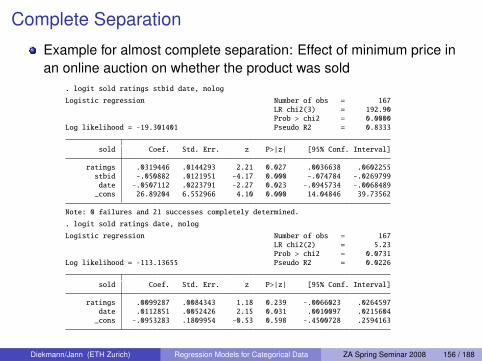
Complete Separation
Example for almost complete separation: Effect of minimum price inan online auction on whether the product was sold
. logit sold ratings stbid date, nolog
Logistic regression Number of obs = 167LR chi2(3) = 192.90Prob > chi2 = 0.0000
Log likelihood = -19.301401 Pseudo R2 = 0.8333
sold Coef. Std. Err. z P>|z| [95% Conf. Interval]
ratings .0319446 .0144293 2.21 0.027 .0036638 .0602255stbid -.050882 .0121951 -4.17 0.000 -.074784 -.0269799date -.0507112 .0223791 -2.27 0.023 -.0945734 -.0068489_cons 26.89204 6.552966 4.10 0.000 14.04846 39.73562
Note: 0 failures and 21 successes completely determined.
. logit sold ratings date, nolog
Logistic regression Number of obs = 167LR chi2(2) = 5.23Prob > chi2 = 0.0731
Log likelihood = -113.13655 Pseudo R2 = 0.0226
sold Coef. Std. Err. z P>|z| [95% Conf. Interval]
ratings .0099287 .0084343 1.18 0.239 -.0066023 .0264597date .0112851 .0052426 2.15 0.031 .0010097 .0215604_cons -.0953283 .1809954 -0.53 0.598 -.4500728 .2594163
Diekmann/Jann (ETH Zurich) Regression Models for Categorical Data ZA Spring Seminar 2008 156 / 188

Complete Separation or Perfect DeterminationExample: Effect of minimum price in an online auction on whether theproduct was sold
0.2
.4.6
.81
Pr(
Sol
d=1)
0 200 400 600 800Starting bid
Diekmann/Jann (ETH Zurich) Regression Models for Categorical Data ZA Spring Seminar 2008 157 / 188

Collinearity
Complete collinearity: If a predictor is a linear combination of one ormore other predictors in the equation then the single effects cannotbe separated. Example: K dummies for a variable with K categories.
dK = 1 −K−1∑k=1
dk
Almost complete collinearity: If two (or more) covariates are closelyrelated, then there is only little information to separate the effects ofthe covariates (⇒ large standard errors)
The solution to collinearity problems depends on context.I If the variables are different measures for the same: use only one or
use an indexI If variables overlap by definition: create non-overlapping variables
Diekmann/Jann (ETH Zurich) Regression Models for Categorical Data ZA Spring Seminar 2008 158 / 188

CollinearityExample: Effect of net minimum price and gross minimum price in anonline auction (the gross price includes shipping)
. logit sold netminprice grossminprice, nolog
Logistic regression Number of obs = 167LR chi2(2) = 184.47Prob > chi2 = 0.0000
Log likelihood = -23.515457 Pseudo R2 = 0.7968
sold Coef. Std. Err. z P>|z| [95% Conf. Interval]
netminprice .1549288 .0818699 1.89 0.058 -.0055332 .3153908grossminpr˜e -.1935158 .0864308 -2.24 0.025 -.3629171 -.0241146
_cons 24.09443 5.751801 4.19 0.000 12.82111 35.36775
Note: 0 failures and 19 successes completely determined.
. gen shipping = grossminprice - netminprice
. logit sold netminprice shipping, nolog
Logistic regression Number of obs = 167LR chi2(2) = 184.47Prob > chi2 = 0.0000
Log likelihood = -23.515457 Pseudo R2 = 0.7968
sold Coef. Std. Err. z P>|z| [95% Conf. Interval]
netminprice -.038587 .0087499 -4.41 0.000 -.0557365 -.0214376shipping -.1935158 .0864308 -2.24 0.025 -.3629171 -.0241146_cons 24.09443 5.751801 4.19 0.000 12.82111 35.36775
Note: 0 failures and 19 successes completely determined.
Diekmann/Jann (ETH Zurich) Regression Models for Categorical Data ZA Spring Seminar 2008 159 / 188
Part X
Probit and Latent Variable Model
Alternatives to Logit
The Probit Model
Latent Variable Model
Example: Logit versus Probit
Diekmann/Jann (ETH Zurich) Regression Models for Categorical Data ZA Spring Seminar 2008 160 / 188

Alternatives to LogitThe Logit model is
Pr(Y = 1|X) = F(Xβ) =exp(Xβ)
1 + exp(Xβ)
We can use other (typically s-shaped) functions in place of F(Xβ)instead of the logistic function
(Aldrich/Nelson 1984)
Diekmann/Jann (ETH Zurich) Regression Models for Categorical Data ZA Spring Seminar 2008 161 / 188

The Probit ModelOne such alternative is the Probit model which uses the cumulativenormal distribution
Pr(Y = 1|X) = Φ(Z) =
∫ Z
−∞
1√
2πexp(−u2/2) du
or: Φ−1(Pr(Y = 1|X)) = β0 + β1X1 + · · ·+ βmXm
The Logit and Probit are very similar:
-4 -3 -2 -1 0 1 2 3 40
0.5
1
X
P
standard normalstandard logisticstandardised logistic
Diekmann/Jann (ETH Zurich) Regression Models for Categorical Data ZA Spring Seminar 2008 162 / 188

The Probit Model
Interpretation is of coefficients is similar to the Logit model
Marginal effect:
∂Pr(Y = 1|X)
∂Xk=
[1√
2πexp(−Z2/2)
]βj = φ(Z)βj
Discrete change effect:
∆ Pr(Y = 1|X)
∆Xj= Φ[· · ·+ βk (Xk + 1) + · · · ] − Φ[· · ·+ βk Xk + · · · ]
Diekmann/Jann (ETH Zurich) Regression Models for Categorical Data ZA Spring Seminar 2008 163 / 188

Latent Variable Model
The Probit model and the Logit model can be expressed as latentvariable models.
The conceptual idea is that there is an unobserved variable Y∗ thatreflects the propensity of Y to take on value 1 and is related to thecovariates in a linear way.
The model is:
Y∗ = Xβ+ ε with Y =
1 if Y∗ > 0
0 if Y∗ ≤ 0
Discrete choice models: Y∗ can be interpreted as the differencebetween the utilities of the two alternatives (plus error)
Diekmann/Jann (ETH Zurich) Regression Models for Categorical Data ZA Spring Seminar 2008 164 / 188

Latent Variable Model
(Long 1997)
Diekmann/Jann (ETH Zurich) Regression Models for Categorical Data ZA Spring Seminar 2008 165 / 188

Latent Variable Model
Expressed this way, the only difference between the Logit model andthe Probit model then is that they make a different assumption aboutthe distribution of ε
Probit: ε has a standard normal distribution, N(0, 1)
Logit: ε has a standard logistic distribution, exp(ε)/[1 + exp(ε)]
The standard deviation of ε in the Logit model is π/√
3. Therefore thecoefficients from the Logit model are usually about π/
√3 ≈ 1.8 times
larger than the coefficients from the Probit model.
Logit versus Probit
βLogit ≈ 1.8 · βProbit
Diekmann/Jann (ETH Zurich) Regression Models for Categorical Data ZA Spring Seminar 2008 166 / 188

Example: Logit versus Probit
. estout, cells("b Xmfx_dydx(label(MargEfct))" "t(par)")
LOGIT PROBITb/t MargEfct b/t MargEfct
educ .1493077 .0285554 .0791481 .0258561(3.673453) (3.582843)
age -.0380774 -.0072824 -.020756 -.0067806(-5.212636) (-5.211616)
k5 -1.171423 -.2240373 -.6776337 -.2213693(-8.855418) (-9.153815)
k618 -.2328272 -.0445287 -.1340417 -.0437887(-2.983747) (-2.888898)
protestant .1803333 .0344891 .1072967 .0350517(1.201285) (1.217839)
inc1000 -.066502 -.0127187 -.0405756 -.0132552(-3.474943) (-3.585695)
_cons 1.490499 .9182765(2.62552) (2.928594)
Diekmann/Jann (ETH Zurich) Regression Models for Categorical Data ZA Spring Seminar 2008 167 / 188

Part XI
Generalizations
Ordered Logit/Probit
Multinomial Logit
Conditional Logit
Diekmann/Jann (ETH Zurich) Regression Models for Categorical Data ZA Spring Seminar 2008 168 / 188

More Than Two Categories
Up to now we assumed that Y , the dependent variable, has only twovalues, 0 and 1.
The discussed approaches can be generalized to polytomousvariables with more than two values.
Diekmann/Jann (ETH Zurich) Regression Models for Categorical Data ZA Spring Seminar 2008 169 / 188

Ordered Logit/Probit
The values of Y have a natural order.
Examples:I “How satisfied are you with your life?” 1 = “not at all”, 2 = “a bit’, 3 =
“very much”I Social class: lower, middle, upper
Such variables are often analyzed using linear regression.
However, linear regression makes the assumption that the “distances”between the categories are the same.
Since this assumption may be wrong, linear regression might bebiased, and it is worthwhile to analyze such data using techniquesthat do not assume interval data.
In general, using linear regression is less problematic if Y has manyvalues.
Diekmann/Jann (ETH Zurich) Regression Models for Categorical Data ZA Spring Seminar 2008 170 / 188

Ordered Logit/Probit
Ordered Logit/Probit can be represented using the latent variablemodel.
Y∗ = β0 + β1X1 + · · ·+ βmXm + ε
with
Y =
1 if Y∗ < τ12 if τ1 ≤ Y∗ < τ2· · ·
J if τJ−1 ≤ Y∗
τ1, . . . , τJ−1 are the thresholds that map the continuous Y∗ to thediscrete Y
(Long 1997)
Diekmann/Jann (ETH Zurich) Regression Models for Categorical Data ZA Spring Seminar 2008 171 / 188

Ordered Logit/Probit
The difference between ordered Logit and ordered Probit lies again inthe assumed distribution for the error term.
I Probit: ε has a standard normal distributionI Logit: ε has a standard logistic distribution
(Long 1997)
Diekmann/Jann (ETH Zurich) Regression Models for Categorical Data ZA Spring Seminar 2008 172 / 188

Ordered Logit/Probit: Interpretation
The raw coefficients of ordered Logit/Probit are expressed in terms ofthe latent variable Y∗.
The signs of the coefficients have a clear interpretation: If the effect ispositive, the probability Y to take on a higher value increases (andvice versa).
In the case of the ordered Logit an odds ratio interpretation ispossible: If Xk is increased by one unit, then the odds of Y beingequal to j or less are changed by factor exp(−βk ).
For detailed interpretation, marginal effects and discrete changeeffects on the probabilities of the categories can be computed (seeLong 1997 for details). However, note that these effects are categoryspecific (separate effect for each category).
Diekmann/Jann (ETH Zurich) Regression Models for Categorical Data ZA Spring Seminar 2008 173 / 188

Ordered Logit/Probit: InterpretationThe probability of Y = j given variables X is
Pr(Y = j|X) = F(τj − Xβ) − F(τj−1 − Xβ)
where τ0 = −∞ and τj = ∞ and F() denotes the cumulative normaldistribution or logistic.Marginal effect
∂Pr(Y = j|X)
∂Xk= βk [f(τj−1 − Xβ) − f(τj − Xβ)]
Discrete change
∆ Pr(Y = j|X)
∆Xk= F(τj−· · ·−βk (Xk +1)−. . . )−F(τj−1−· · ·−βk Xk −. . . )
Note that the sign of a marginal effect or discrete change effect maybe different than the sign of βk . The sign may even change over therange of Xk .
Diekmann/Jann (ETH Zurich) Regression Models for Categorical Data ZA Spring Seminar 2008 174 / 188

Ordered Logit/Probit: Example. fre weffort, nomissing
weffort work effort beyond what is required
Freq. Percent Cum.
1 none 124 6.01 6.012 only a little 175 8.49 14.503 some 927 44.96 59.464 a lot 836 40.54 100.00Total 2062 100.00
. esttab, mtitles eqlabels(none) wide compress
(1) (2) (3)LRM OPROBIT OLOGIT
female 0.106* (2.50) 0.147* (2.50) 0.229* (2.33)parttime -0.303*** (-6.57) -0.418*** (-6.62) -0.704*** (-6.56)selfemp 0.224*** (4.19) 0.374*** (4.91) 0.688*** (5.28)educ 0.0158* (2.02) 0.0194 (1.81) 0.0300 (1.65)_cons 3.027*** (31.20)cut1 -1.365*** (-9.96) -2.469*** (-10.33)cut2 -0.862*** (-6.40) -1.484*** (-6.47)cut3 0.464*** (3.47) 0.733** (3.23)
N 2062 2062 2062
t statistics in parentheses* p<0.05, ** p<0.01, *** p<0.001
Diekmann/Jann (ETH Zurich) Regression Models for Categorical Data ZA Spring Seminar 2008 175 / 188

Multinomial Logit
Nominal variable: The categories have no natural order.
The multinomial Logit is used for nominal variables or for orderedvariables where the ordering is questionable (e.g. occupationalattainment)
The model has many parameters! There is one set of parameters foreach category of Y .
Diekmann/Jann (ETH Zurich) Regression Models for Categorical Data ZA Spring Seminar 2008 176 / 188

Multinomial Logit
The probabilities of the different outcomes of Y are expressed as
Pr(Y = j|X) =exp(Xβj)∑J`=1 exp(Xβ`)
with β set to zero for one of the outcomes.
The outcome for which the β vector is set to zero is called the “baseoutcome” or the “reference category”
The parameter estimates of the multinomial Logit therefore expressdifferences compared to the base outcome.
Note that the binary Logit model is a special case of the multinomialLogit.
Diekmann/Jann (ETH Zurich) Regression Models for Categorical Data ZA Spring Seminar 2008 177 / 188

Multinomial Logit: Odds
The odds of outcome j versus outcome m are
Pr(Y = j|X)
Pr(Y = m|X)=
Pj
Pm=
exp(Xβj)∑J`=1 exp(Xβ`)
exp(Xβm)∑J`=1 exp(Xβ`)
=exp(Xβj)
exp(Xβm)
Taking the logarithm yields
ln(Pj/Pm) = X(βj − βm)
and the partial derivative is:
∂ ln(Pj/Pm)
∂Xk= βkj − βkm
Diekmann/Jann (ETH Zurich) Regression Models for Categorical Data ZA Spring Seminar 2008 178 / 188

Multinomial Logit: Odds
The parameters in the multinomial Logit can therefore be interpretedas follows.
Log Odds: If Xk is increased by one unit the log of the odds ofoutcome j against outcome m changes by βkj − βkm.
Odds: If Xk is increased by one unit the odds of outcome j againstoutcome m (the “relative risk ratio”) changes by factor exp(βkj − βkm).If m is the base outcome: βkm = 0
I Log Odds: If Xk is increased by one unit the log of the odds of outcomej against the base outcome changes by βkj .
I Odds: If Xk is increased by one unit the odds of outcome j against thebase outcome changes by exp(βkj).
Diekmann/Jann (ETH Zurich) Regression Models for Categorical Data ZA Spring Seminar 2008 179 / 188

Multinomial Logit: Partial Effect and Discrete Change
Also for the multinomial Logit we can compute marginal effects anddiscrete change effects. Similar to the ordered Logit/Probit, thedirection of these effects may not correspond to the signs of thecoefficients and the direction may also depend on the values of thecovariates for which the effects are computed.
Recall that Pr(Y = j|X) = exp(Xβj)/∑J`=1 exp(Xβ`)
Partial effect:
∂Pr(Y = j|X)
∂Xk= Pr(Y = j|X)
βkj −
J∑`=1
βk` Pr(Y = `|X)
Discrete change:
∆ Pr(Y = j|X)
∆Xk= Pr(Y = j|X ,Xk + 1) − Pr(Y = j|X)
Diekmann/Jann (ETH Zurich) Regression Models for Categorical Data ZA Spring Seminar 2008 180 / 188

Multinomial Logit: Example
Labor force status by sex and education
. fre lfstatus, nomissing
lfstatus
Freq. Percent Cum.
1 full time 1267 44.60 44.602 part time 538 18.94 63.53
3 selfemployed 285 10.03 73.57
4 not in labor force 751 26.43 100.00Total 2841 100.00
Diekmann/Jann (ETH Zurich) Regression Models for Categorical Data ZA Spring Seminar 2008 181 / 188
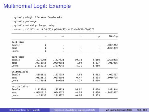
Multinomial Logit: Example
. quietly mlogit lfstatus female educ
. quietly prchange
. quietly estadd prchange, adapt
. estout, cell("b se t(fmt(2)) p(fmt(3)) dc(label(DisChg))")
b se t p DisChg
full timefemale 0 . . . -.4035242educ 0 . . . .0224239_cons 0 . . .
part timefemale 2.76204 .1427824 19.34 0.000 .2668968educ .0272368 .0250682 1.09 0.277 .017066_cons -2.856912 .3279246 -8.71 0.000
selfemployedfemale .4184821 .1375259 3.04 0.002 -.052557educ .0128819 .0274198 0.47 0.638 .0086798_cons -1.78688 .340294 -5.25 0.000
not in lab˜efemale 1.725244 .1025924 16.82 0.000 .1891844educ -.0981816 .0243676 -4.03 0.000 -.0481697_cons -.28136 .2915872 -0.96 0.335
Diekmann/Jann (ETH Zurich) Regression Models for Categorical Data ZA Spring Seminar 2008 182 / 188

Conditional Logit
The conditional Logit is a variant on the multinomial Logit that can beapplied if the data contain alternative specific information.
I Multinomial Logit: X variables are characteristics of the individuals;they vary over individuals
I Conditional Logit: Additional variables Z that reflect characteristics ofthe categories of Y (the “alternatives”)
Examples are the traffic mode choice where travel costs and time areknown for each mode or the choice of consumer goods or serviceswhere various characteristics of the good or service are known.The shape of the data set is different for conditional Logit than formultinomial Logit:
I Multinomial Logit: one row per individualI Conditional Logit: one row per alternative (including a variable
identifying the individual and a variable indicating the chosenalternative)
Diekmann/Jann (ETH Zurich) Regression Models for Categorical Data ZA Spring Seminar 2008 183 / 188

Conditional Logit
The probability of choosing alternative J given variables X that varyby individual and variables Z that vary by alternative (and individual)is expressed as
Pr(Y = j|X ,Z) =exp(Xβj + Zjγ)∑J`=1 exp(Xβ` + Z`γ)
Odds interpretation of γ: If the difference in Zk between alternative jand alternative m is increased by 1 unit then the odds of alternative jover alternative m change by factor exp(γk )
Diekmann/Jann (ETH Zurich) Regression Models for Categorical Data ZA Spring Seminar 2008 184 / 188

Further Topics
Models for count data
Models for limited or truncated data
Complex samples, weights
Panel data models, multilevel models
GLM (Generalized Linear Models)
Log-linear models
Nonparametric methods
Causal inference, endogeneity, sample selection correction
Diekmann/Jann (ETH Zurich) Regression Models for Categorical Data ZA Spring Seminar 2008 185 / 188

Additional References
References cited in the lectures but not listed in textbooks section:
Bagley, Steven C., Halbert White, and Beatrice A. Colomb (2001). Logisticregression in the medical literature: Standards for use and reporting, with particularattention to one medical domain. Journal of Clinical Epidemiology 54: 979-985.
Berkson, Joseph (1944). Application of the Logistic Function to Bio-Assay. Journal ofthe American Statistical Association 39(227): 357-365.
Berkson, Joseph (1951). Why I Prefer Logits to Probits. Biometrics 7(4): 327-339.
Caudill, Steven B. (1988). An Advantage of the Linear Probability Model over Probitor Logit. Oxford Bulletin of Economics & Statistics 50(4): 425-427.
Fox, John (1991). Regression Diagnostics. Newbury Park, CA: Sage.
Fox, John (2000). Nonparametric Simple Regression. Smoothing Scatterplots.Thousand Oaks, CA: Sage.
Gelman, Andrew, and Hal Stern (2006). The Difference Between “Significant” and“Not Significant” is not Itself Statistically Significant. The American Statistician 60(4):328-331.
Diekmann/Jann (ETH Zurich) Regression Models for Categorical Data ZA Spring Seminar 2008 186 / 188

Goldberger, Arthur Stanley (1964). Econometric Theory. New York: John Wiley &Sons.
Golding, Jean, Rosemary Greenwood, Karen Birmingham, and Martin Mott (1992).Childhood cancer, intramuscular vitamin K, and pethidine given during labour. BMJ305: 341-346.
Hosmer, David W., and Stanley Lemeshow (1980). Goodness of fit tests for themultiple logistic regression model. Communications in Statistics - Theory andMethods 9(10): 1043 - 1069.
Jann, Ben (2005). Comment: Earnings Returns to Education in Urban China: A Noteon Testing Differences among Groups. American Sociological Review 70(5):860-864.
Jann, Ben (2006). Diagnostik von Regressionsschatzungen bei kleinen Stichproben.Kolner Zeitschrift fur Soziologie und Sozialpsychologie Sonderheft 44/2004:421-452.
Kruskal, William H. (1960). Some Remarks on Wild Observations. Technometrics2(1): 1-3.
Diekmann/Jann (ETH Zurich) Regression Models for Categorical Data ZA Spring Seminar 2008 187 / 188

Lemeshow, Stanley, and David W. Hosmer, Jr. (1982). A Review of Goodness of FitStatistics for Use in the Development of Logistic Regression Models. AmericanJournal of Epidemiology 115(1): 92-106.
Peduzzi, Peter, John Concato, Elizabeth Kemper, Theodore R. Hiolford, and Alvan R.Feinstein (1996). A Simulation Study of the Number of Events per Variable in LogisticRegression Analysis. Journal of Clinical Epidemiology 49(12): 1373-1379.
Petersen, Trond (1985). A Comment in Presenting Results from Logit and ProbitModels. American Sociological Review 50(1): 130-131.
Pregibon, Daryl (1981). Logistic Regression Diagnostics. The Annals of Statistics9(4): 705-724.
Smith, Gordon C. S., and Jill P. Pell (2003). Parachute use to prevent death andmajor trauma related to gravitational challenge: systematic review of randomisedcontrolled trials. BMJ 327: 1459-1461.
Diekmann/Jann (ETH Zurich) Regression Models for Categorical Data ZA Spring Seminar 2008 188 / 188